Mechanical factors affecting the mobility of membrane proteins

Abstract

The mobility of membrane proteins controls many biological functions. The application of the model of Saffman and Delbrück to the diffusion of membrane proteins does not account for all the experimental measurements. These discrepancies have triggered a lot of studies on the role of the mechanical factors in the mobility. After a short review of the Saffman and Delbrück model and of some key experiments, we explore the various ways to incorporate the effects of the different mechanical factors. Our approach focuses on the coupling of the protein to the membrane, which is the central element in the modelling. We present a general, polaron-like model, its recent application to the mobility of a curvature sensitive protein, and its various extensions to other couplings that may be relevant in future experiments.

1 Introduction

Cell membranes are barriers that separate the cytoplasm from the external world. Through compartmentalization, they allow highly selective biochemical reactions to take place in their internal volume which would essentially never occur in the absence of such barriers. Far from being inert, biological membranes thus play a key role in many functions such as signaling, cell division, or energy production in cellular organelles.

Many of these biological functions involve membrane proteins, which form a vast family of essential proteins. While some of them are embedded permanently in the membrane, others transiently bind to it in order to perform a specific task and then unbind from it when the task is done. When they are inserted in the membrane, membrane proteins typically diffuse laterally in the fluid environment of the lipid membrane. This lateral diffusion is an essential aspect to their function, in the frequent case that membrane proteins must interact or form clusters with other membrane proteins. Membrane proteins typically diffuse in a crowded environment of other lipids and proteins. Modeling the various factors (mechanical or biochemical) affecting the mobility of membrane proteins is a challenging issue, but one that should be addressed in order to properly understand their biological function.

In this chapter, we review some of the experiments and theories, which have been devoted to the mobility of membrane proteins. In the next section 2, we present the pioneering work of P. G. Saffman and M. Delbrück (SD) on the mobility of membrane proteins, which is followed in section 3 by a discussion of the experiments which have either tested the model or pointed out its limitations. In section 4, we investigate the crucial couplings between the membrane protein and the membrane. Then, in section 5 we present some of the main theoretical ideas or models which have been put forward to understand the mobility of membrane proteins beyond the SD model. We end up with a discussion on future perspectives.

2 The Saffman and Delbrück hydrodynamic model (SD)

Brownian motion plays an essential role in biological processes. Since the work of Einstein Einstein1905 and the pioneering experiments of Perrin Perrin1909 , the observation of diffusing objects has emerged as a mean to extract the rheological properties of the surrounding medium or the probe particle size. The theoretical investigation of diffusion of proteins within membranes has been studied widely going back to P. G. Saffman and M. Delbrück (SD). They investigated the hydrodynamic drag acting on a membrane inclusion of radius $a_{\mathrm{p}}$ moving in a membrane described as a two dimensional fluid sheet of viscosity $\mu_{\mathrm{m}}$; which is itself in contact with a less viscous fluid of viscosity $\eta$ Saffman1975 . The two dimensional surface viscosity of the membrane $\mu_{\mathrm{m}}$ is the product of the membrane thickness $h$ by its three dimensional viscosity $\eta_{\mathrm{m}}$, $\mu_{\mathrm{m}}=h\eta_{\mathrm{m}}$. The velocity field inside the membrane is exactly two-dimensional but it is hydrodynamically coupled to the external fluid. Using singular perturbation techniques, which are valid when $\eta_{\mathrm{m}}h\gg\eta a_{\mathrm{p}}$, Saffman and Delbrück (SD) obtained the diffusion coefficient $D_{0}$ for the translational Brownian motion of a cylindrical inclusion of radius $a_{\mathrm{p}}$ in the membrane:

$$D_{0}=\frac{k_{B}T}{4\pi\mu_{\mathrm{m}}}\left[\log\left(\frac{\ell}{a_{\mathrm{p}}}\right)-\gamma\right],$$ (1)

where $k_{B}T$ is the thermal energy, $\gamma$ is Euler’s constant and $\ell=\mu_{\mathrm{m}}/\eta$ is the SD length. The expression (1) corresponds to the choice of a no-slip boundary condition at the surface of the inclusion; for the alternate choice of zero tangential stress boundary condition, a factor $1/2$ should be added inside the bracket. Saffman and Delbrück also derived an expression for the rotational diffusion coefficient, which unlike the translational diffusion coefficient only depends on the viscosity of the membrane: $D_{R}=k_{B}T/4\pi h\mu_{\mathrm{m}}a_{\mathrm{p}}^{2}$.

The SD dimensionless parameter $\epsilon=\ell/a_{\mathrm{p}}$ represents physically the ratio of the hydrodynamic resistances of the inclusion in the fluid membrane and in the external fluid. Indeed the former is of the order of the lateral area of the inclusion $2\pi a_{\mathrm{p}}h$ times the membrane shear stress $v\eta_{\mathrm{m}}/a_{\mathrm{p}}$ for a velocity $v$ of the inclusion; while the latter is of the order of the top cylindrical area $\pi a_{\mathrm{p}}^{2}$ times the shear stress in the fluid, $v\eta/a_{\mathrm{p}}$. When $\epsilon\gg 1$, the hydrodynamic resistance due to the motion in the membrane dominates; this is the regime considered by Saffman and Delbrück, which is relevant for small inclusions ($\it i.e.$ for small values of the radius of the inclusion $a_{p}$, which is the only lateral length scale considered in the model). Instead, when $\epsilon\ll 1$, the resistance occurs mainly due to the motion in the external fluid; this is the regime relevant for large inclusions. In this case, since the motion mainly occurs in the bulk external fluid, it is described by the Stokes-Einstein formula, with a mobility going as $1/a_{\mathrm{p}}$. We therefore expect a cross-over between both regimes, when the size of the inclusion is of the order of $500$ nm, which is the estimate for $\ell$ for a typical ratio of viscosities $\eta_{\mathrm{m}}/\eta\simeq 100$ and a membrane thickness $h\simeq 5$ nm.

3 Experimental tests of the Saffman-Delbrück model

Theoretically, a more complete solution of the SD hydrodynamic problem has been proposed which interpolates between the SD regime and the Stokes-Einstein regime Hughes1981 . Such expressions have been tested using simulations Guigas2008 , and later improved by the group of P. Schwille Petrov2008 who also carried out a set of careful experiments with micron-sized solid domains in giant unilamellar vesicles, confirming the results expected in the regime $\epsilon\ll 1$ Petrov2012 .

Below, we focus on some of the experiments which have tested or challenged the SD model in the regime of small inclusions $\epsilon\gg 1$ and for flat membranes, which are conditions for which the model should be applicable. In 2006, Gambin et al. Gambin2006 performed experiments with a large panel of peptides and membrane proteins with various shapes and particle sizes ranging from 5 nm to 30 nm; the diffusion coefficient has been measured using fringe pattern photobleaching. They reported a dependence of the diffusion coefficient on the size of the particle of the Stokes type ($D_{0}\sim 1/a_{\mathrm{p}}$, see Fig. 1), much stronger than the logarithmic dependence predicted by Eq. 1. In a second set of experiments, Gambin et al. tuned the membrane thickness by swelling the membrane with an hydrophobic solvent, and measured the effect on the mobility of the peptides. They found that the mobility of the inclusions is maximal when their height matches the membrane thickness. They attributed the reduced mobility of peptides with a smaller length than the bilayer thickness to the pinching of the bilayer (provided that the peptides are sufficiently long to span the bilayer). On the other hand, peptides much longer than the membrane thickness cannot fit in the upright position and must tilt with respect to the membrane normal, which may cause, again, a reduction of their mobility. These experiments triggered a lot of activity on the theoretical side, which we review in the theory section.

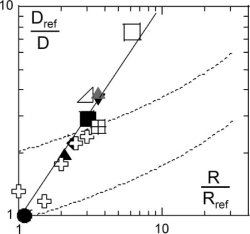
Figure 1: Figure taken from Ref. Gambin2006 : Normalized inverse diffusion coefficient $D_{ref}/D$ vs. object radius $R/R_{ref}$, with open symbols representing data gathered from the literature, and filled symbols data from Ref. Gambin2006 . Filled symbols represent peptides assemblies, with the peptide called $L_{12}$ as reference, while for oligomers of peptides (crosses), acetylcholine receptor (AChR), bacteriorhodopsin (BR), and SR-ATPase (squares), the lipid diffusion serves as reference. The solid line is a power-law regression leading to $D_{ref}/D\sim R^{1.04}$. For comparison, the dashed line represents the prediction of the Saffman–Delbrück model (Eq. 1) (upper line, same as in Fig. 3, and lower fit as in Fig. 2 of Ref. Gambin2006 ).

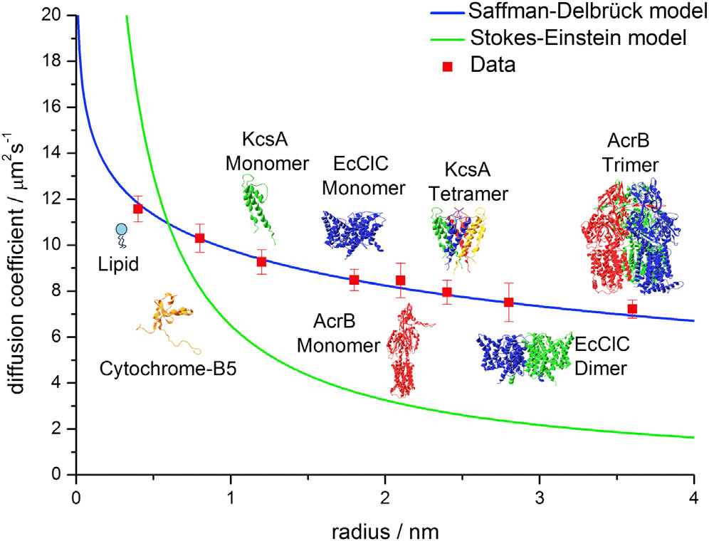
Figure 2: Figure taken from Ref. Weis2013 : Saffman–Delbrück versus Stokes-Einstein model. The investigated species are DPPE, cytochrome B5 (depicted without transmembrane domain), KcsA, EcClC, and AcrB. The monomeric forms of membrane proteins were directly added to the BLM. The oligomeric forms were reconstituted via SNARE-mediated vesicle fusion. DPPE was labeled with Atto655, and all proteins were labeled with Alexa647. In addition, we fitted the HPW-based model suggested by Petrov and Schwille Petrov2008 , which can reproduce the classical Saffman–Delbrück model in the size range investigated. The fit parameter for all fits was the product of membrane viscosity and thickness, $\eta_{\mathrm{m}}h$. The temperature was set to 295 K and the viscosity of the surrounding buffer was $\eta=0.96$ mPa.

In contrast to these experiments, one work Ramadurai2009 reported a weak dependence of $D_{0}$ on the protein radius $a_{\mathrm{p}}$, using fluorescence correlation spectroscopy (FCS) in line with the predictions of the SD model from Eq. 1. The discrepancy with the data of Gambin et al. is likely to come from differences in the experimental techniques which have been used in both cases. Recently, Weiss et al. performed experiments with dual focus fluorescence correlation spectroscopy Weis2013 , which provided accurate measurements, of higher quality than with simple FCS. These more accurate measurements of diffusion coefficients for membrane proteins in black lipid membranes are in perfect agreement with the SD model. The original figure of Ref. Weis2013 is reproduced here in Fig. 2 with courtesy of J. Enderlein. We believe that the reason for this perfect agreement may be that these experiments have been performed with black lipid membranes, which are tense membranes.

The idea that the membrane tension may affect the protein mobility, has only been investigated recently in a study involving one of us Quemeneur2014 . In this work, the mobility of two transmembrane proteins with the same lateral size, aquaporin 0 (AQP0) and a voltage-gated potassium channel (KvAP), have been measured by attaching quantum dots to these proteins and by tracking them. One advantage of using this technique of single particle tracking is that it is free of the possible artifacts due to averaging over a population of interacting proteins (on which the experiments reported in Refs. Gambin2006 ; Gambin2010 rely). Whereas AQP0 does not deform the bilayer, KvAP is curved and bends the membrane. These experiments have shown that the curvature-coupled protein KvAP undergoes a significant increase in mobility under tension – an effect clearly beyond the SD model – , whereas the mobility of the curvature-neutral water channel AQP0 is insensitive to it and follows the prediction of the SD model, as shown in Fig. 3. Importantly, at high tension, the mobility of both proteins agree well with the prediction of the SD model, which gives $D_{0}=2.5$ $\mu\mathrm{m}^{2}/\mathrm{s}$ Gambin2006 .

So far, we have only discussed proteins diffusing in flat membranes. However, the SD model has also been tested using the same technique of single particle tracking and the same protein KvAP, but in different membrane environments namely in the curved and confined space of membrane nanotubes Domanov2011 . In this work, it was found that measurements of the mobility of this protein in the tube are well described by an extension of the SD model to cylindrical geometries Daniels2007 .

Finally, let us mention some applications of the SD model for microrheology. Similarly to the Einstein relation, which allows the determination of the 3D local viscosity, based on measurements of the fluctuations of one or two tracers in a bulk fluid, the SD relation allows the determination of local membrane viscosity from measurements of the fluctuations of a tracer. This tracer can be a protein, but in that case it is crucial to properly understand the coupling between the protein and the membrane, as emphasized in the present chapter. In order to disentangle effects due to the tracer and the membrane, it is helpful if possible to combine measurements of translation or rotation diffusion as shown in Ref. Hormel2014 .

4 Relevant geometrical or mechanical factors and protein-membrane couplings

Various geometrical or mechanical factors can affect the mobility of membrane proteins. The main factors are listed below:

• Geometrical properties of the membrane. The most basic geometrical parameter of the membrane is its thickness. For lipid membranes, this parameter is generally assumed to be constant of the order of 4 to 5nm. However, biological membranes are intrinsically heterogeneous and usually composed of mixtures of several kinds of lipid domains. In such systems, the membrane thickness can vary depending on the location inside or outside the domains. Another very important local geometrical property of the membrane is its curvature. A preference of certain membrane proteins for membrane curvature means in particular that it is possible to sort them according to the local curvature as demonstrated in Ref. Aimon2014 .

• Mechanical and chemical properties of the membrane. The former ones include the elastic moduli of the membrane, such as its bending modulus and its tension, and dissipative moduli, such as the membrane viscosity and the relative friction between membrane leaflets. The latter ones include the chemical composition of the membrane, which controls many of its properties. Both parameters should be regarded as local or global depending on the level of heterogeneity.

• Geometrical parameters and mechanical properties of the membrane protein. The geometrical parameters of the protein include its size and shape Chang1998 ; Liu2009 ; Camley2013 ; Aimon2014 . Its shape notably defines its spontaneous curvature, which is a scalar for isotropic inclusions but becomes a tensor for anisotropic ones. Other important protein mechanical properties include its compliance, which can be split into elastic and dissipative moduli.

• The solvent in which the protein and the membrane are embedded. It is mainly characterized by its viscosity which controls the hydrodynamic part of the dissipation. In the case that the membrane and its solvent are confined by rigid walls, the solvent will be also described by its thickness, which can affect the mobility of membrane proteins via hydrodynamic screening effects Seki2011 ; Stone1998 .

• Other inclusions present in the membrane modify the mobility of a given membrane protein, via direct interactions such as exclusion or indirect ones, such as membrane mediated interactions Goulian1993 ; Reynwar2008 . Since at the microscopic scale, biological membranes are a crowded mix of membrane proteins and lipid partners, such collective effects are expected to be important.

In order to understand the way mechanical factors affect the mobility of a given protein, it is important to focus on the mechanism by which the protein couples to the membrane. The main coupling mechanisms are:

• Hydrodynamic coupling. Since the protein evolves in the membrane which is fluid, there is a clear hydrodynamic coupling due to the fluid membrane. But since the external fluid may be dragged by the motion of the lipids induced by the protein, there is also hydrodynamic coupling with the external fluid, which is usually water. This is the coupling considered by Saffman and Delbrück Saffman1975 and in Seki2011 ; Stone1998 .

• Coupling to the local membrane curvature. A mismatch between the spontaneous curvature of the protein and the curvature of the membrane deforms the lipids around the protein, leading to an energetic penalty Goulian1993 ; Reister2005 ; Reynwar2007 ; Naji2009 ; Quemeneur2014 . The precise form of this coupling depends whether the protein is assumed to be hard or soft.

• Coupling to the membrane thickness. A hydrophobic mismatch between the protein and the membrane thickness stretches or compresses the lipid tails around the protein Andersen2007 .

• Coupling to the membrane composition. Such an effect will be present when the protein has a special affinity for one kind of lipids while the membrane is made of a mix of various lipids Reynwar2008 .

• Electrostatic coupling. Various mechanisms are possible, depending whether the protein and the lipids are charged or not. Note that even if the lipids are uncharged, such couplings may be present since the lipids may be polarized locally by the protein if the later is charged. For membrane ion channels, there is generally a coupling of electrostatic origin in the presence of a transmembrane voltage since the field lines are deformed locally near the protein Winterhalter1987 . Such a coupling is involved in the mechanism of voltage gating in ion channels Phillips2009 .

• Coupling due to geometrical effects. This form of coupling arises because the real trajectories of membrane proteins occur in 3D whereas these trajectories are typically recorded experimentally in a 2D space Reister2005 ; Reister-Gottfried2007 . This projection of real trajectories on 2D space results in an additional reduction of the protein mobility.

Naturally, a given protein may couple to the membrane via several couplings of this kind simultaneously, and more couplings are possible. In the next section, we explore non-hydrodynamic couplings, and their consequences for the mobility of the membrane protein.

5 Theoretical models

SD theory implicitly assumes that the protein diffuses in a membrane which remains flat and unaffected by the presence of the protein. Therefore, a possible origin for the discrepancy observed by Gambin et al. Gambin2006 is the significant local membrane deformation due to the interaction between the protein and the lipid bilayer as proposed in 2007 by Naji et al. Naji2007 . In this view, a given membrane protein should experience additional dissipation, either within the membrane or within the external fluid, due to the local deformation which it carries along as it diffuses in the membrane.

In the next subsection, we sketch the original theoretical argument put forward by Naji et al. Then, we turn to a more formal analysis of the drag coefficient for a general order parameter using the so called polaron model. In the next subsection, this polaron model is applied to the specific membrane curvature coupling and used to analyze the experiments of Ref. Quemeneur2014 . We finish with other potential applications of this framework and with a list of open problems.

5.1 Heuristic approach to the membrane perturbation

Naji et al. suggested that the discrepancy between the SD prediction Saffman1975 and the experimental results of Gambin et al. Gambin2006 could be attributed to the perturbation of a local order parameter $\phi(\mathbf{r})$ of the membrane that could represent its lipid composition, thickness, or height Naji2007 . They assumed that the perturbation of the order parameter $\phi$ has a characteristic length $\xi$, and is dragged along with the protein, dissipating energy in a boundary layer of width $\delta\xi$. The power dissipated by this process is $P_{\phi}\sim 2\pi(a_{\mathrm{p}}+\xi)\delta\xi v^{2}$, corresponding to a drag coefficient

$$\lambda_{\phi}\sim 2\pi(a_{\mathrm{p}}+\xi)\delta\xi.$$ (2)

If the length scale of the perturbation is small with respect to the size of the protein, $\xi\ll a_{\mathrm{p}}$, the drag coefficient takes the form $\lambda_{\phi}=\Gamma a_{\mathrm{p}}$. This drag coefficient enters the Einstein relation for the diffusion coefficient together with the SD drag $\lambda_{\mathrm{SD}}$, giving

$$D=\frac{kT}{\lambda_{\mathrm{SD}}+\lambda_{\phi}}=\frac{kT}{\lambda_{\mathrm{SD}}+\Gamma a_{\mathrm{p}}}.$$ (3)

If the dissipation due to the perturbation of the order parameter $\phi$ dominates, the diffusion coefficient scales as $D\sim 1/a_{\mathrm{p}}$, which is compatible with the experiments of Gambin et al. Gambin2006 .

In the following subsection, we turn to a formal description of the perturbation of the order parameter $\phi$, which allows to compute the drag coefficient precisely.

5.2 A polaron model for the perturbation of an order parameter

The back-action on an object that modifies its environment generates a drag force known as the polaron effect, which was originally described for an electron moving in a lattice Landau1933 . A polaron is a charge carrier which deforms a surrounding lattice and moves in it with an induced polarization field. This effect has been applied to soft matter systems by one of us Demery2010 ; Demery2010a . We recall briefly the steps that allow to compute the drag coefficient generated by the coupling between the protein and a local order parameter (or field) $\phi(\mathbf{r})$, which may represent, e.g., the membrane height, thickness, or composition.

Definition of the model

There are two steps in the modeling of the coupling between the protein and the order parameter $\phi(\mathbf{r})$ of the membrane. The first is to write the Hamiltonian of the protein-order parameter system, that we assume to be of the form

$$\mathcal{H}[\phi(\mathbf{r}),\mathbf{R}]=\frac{1}{2}\int\phi(\mathbf{r})\Delta*\phi(\mathbf{r})d^{2}\mathbf{r}-K*\phi(\mathbf{R}),$$ (4)

where the star denotes the convolution product $A*B(\mathbf{r})=\int A(\mathbf{r}-\mathbf{r}^{\prime})B(\mathbf{r}^{\prime})d^{2}\mathbf{r}^{\prime}$.

The first term is the energy of the order parameter itself, it is quadratic in the field and determined completely by the operator $\Delta(\mathbf{r})$. The second term couples the order parameter to the position of the protein, it is linear in the field and determined by the operator $K(\mathbf{r})$. The second step is to give the dynamics of the field, that we assume to be overdamped,

$$\frac{\partial\phi}{\partial t}(\mathbf{r},t)=-R*\frac{\delta\mathcal{H}}{\delta\phi(\mathbf{r},t)}+\eta(\mathbf{r},t),$$ (5)

where $R(\mathbf{r})$ is a linear operator and $\eta(\mathbf{r},t)$ is a Gaussian white noise with correlation function

$$\left\langle\eta(\mathbf{r},t)\eta(\mathbf{r}^{\prime},t^{\prime})\right\rangle=2TR(\mathbf{r}-\mathbf{r}^{\prime})\delta(t-t^{\prime}),$$ (6)

and $\delta\mathcal{H}/\delta\phi(\cdot,t)$ denotes a functional derivative Chaikin1995_vol .

The presence of the operator $R(\mathbf{r})$ in the noise correlation ensures that detailed balance is satisfied. Under this form, the model is completely determined by the three linear operators $\Delta(\mathbf{r})$, $K(\mathbf{r})$ and $R(\mathbf{r})$.

Computation of the drag coefficient

The force exerted by the field on the protein is given by the gradient of the interaction energy,

$$\mathbf{f}[\phi(\mathbf{r}),\mathbf{R}]=-\nabla_{\mathbf{R}}\mathcal{H}[\phi(\mathbf{r}),\mathbf{R}]=\nabla K*\phi(\mathbf{R}).$$ (7)

To compute the drag coefficient, a constant velocity $\mathbf{v}$ is imposed to the protein, $\mathbf{R}(t)=\mathbf{v}t$. We introduce the average field in the reference frame of the protein, which is time-independent in the stationary regime,

$$\Phi(\mathbf{r})=\langle\phi(\mathbf{r}-\mathbf{R}(t),t)\rangle,$$ (8)

The average drag force can be written as

$$\left\langle\mathbf{f}[\phi(\mathbf{r},t),\mathbf{R}(t)]\right\rangle=\nabla K*\Phi(0).$$ (9)

The average field in the reference frame of the protein is obtained by averaging Eq. 5 in the moving frame:

$$-\mathbf{v}\cdot\nabla\Phi(\mathbf{r})=-R*\Delta*\Phi(\mathbf{r})+R*K(-\mathbf{r}),$$ (10)

This equation is solved in Fourier space,

$$\tilde{\Phi}(\mathbf{k})=\int e^{-i\mathbf{k}\cdot\mathbf{r}}\Phi(\mathbf{r})d^{2}\mathbf{r}=\frac{\tilde{R}(\mathbf{k})\tilde{K}^{*}(\mathbf{k})}{\tilde{R}(\mathbf{k})\tilde{\Delta}(\mathbf{k})-i\mathbf{k}\cdot\mathbf{v}}.$$ (11)

The force can be deduced from this Fourier transform,

$$\langle\mathbf{f}\rangle=\int i\mathbf{k}\tilde{K}(\mathbf{k})\tilde{\Phi}(\mathbf{k})\frac{d^{2}\mathbf{k}}{(2\pi)^{2}}=\int\frac{i\mathbf{k}\tilde{R}(\mathbf{k})\left|\tilde{K}(\mathbf{k})\right|^{2}}{\tilde{R}(\mathbf{k})\tilde{\Delta}(\mathbf{k})-i\mathbf{k}\cdot\mathbf{v}}\frac{d^{2}\mathbf{k}}{(2\pi)^{2}}$$ (12)

Expanding the force at small velocity leads to

$$\langle\mathbf{f}\rangle\underset{|\mathbf{v}|\to 0}{\sim}-\frac{\mathbf{v}}{2}\int\frac{\mathbf{k}^{2}\left|\tilde{K}(\mathbf{k})\right|^{2}}{\tilde{R}(\mathbf{k})\tilde{\Delta}(\mathbf{k})^{2}}\frac{d^{2}\mathbf{k}}{(2\pi)^{2}},$$ (13)

where we used that $\int\mathbf{k}\cdot\mathbf{v}\mathbf{k}f(|\mathbf{k}|)d^{2}\mathbf{k}=\frac{1}{2}\mathbf{v}\int\mathbf{k}^{2}f(|\mathbf{k}|)d^{2}\mathbf{k}$ for any function $f(|\mathbf{k}|)$. The drag coefficient is thus

$$\lambda=\frac{1}{2}\int\frac{\mathbf{k}^{2}\left|\tilde{K}(\mathbf{k})\right|^{2}}{\tilde{R}(\mathbf{k})\tilde{\Delta}(\mathbf{k})^{2}}\frac{d^{2}\mathbf{k}}{(2\pi)^{2}}=\frac{1}{4\pi}\int_{0}^{\infty}\frac{k^{3}\left|\tilde{K}(k)\right|^{2}}{\tilde{R}(k)\tilde{\Delta}(k)^{2}}dk.$$ (14)

The second equality assumes isotropic operators.

If this integral diverges at large wavevectors $k$, the finite size $a_{\mathrm{p}}>0$ of the protein can be used to cut-off the integral at $k_{\mathrm{max}}=\pi/a_{\mathrm{p}}$ Demery2010 ; Demery2010a . This regularization introduces a dependence of the drag on the size of the protein, whose form depends on the divergence of the integral.

The formula (14) involves the three operators that determine the model. We shall see below how it applies to the coupling of the membrane curvature with a protein with spontaneous curvature.

Link to the diffusion coefficient

The Einstein relation Einstein1905 relates the diffusion coefficient $D$ to the drag coefficient $\lambda_{\mathrm{f}}$ defined as the ratio between the constant force applied to the particle and its average velocity, $\mathbf{f}=\lambda_{\mathrm{f}}\langle\mathbf{v}\rangle$ by $D=k_{\mathrm{B}}T/\lambda_{\mathrm{f}}$. In a fluctuating field, the drag coefficient $\lambda_{\mathrm{f}}$ and the drag coefficient $\lambda$ computed at constant velocity are not equal Dean2011 ; Demery2011 . However, in the adiabatic regime where the field equilibrates much faster than the particle, the field remains close to equilibrium and the two drag coefficients are equal Dean2011 ; Demery2011 . In this case, the diffusion coefficient can be written as

$$D_{\mathrm{eff}}=\frac{k_{\mathrm{B}}T}{\lambda_{\mathrm{SD}}+\lambda_{\phi}},$$ (15)

where $\lambda_{\phi}$ is given by Eq. 14.

5.3 Application to a protein that couples to the membrane curvature

The coupling of a protein to the membrane curvature and its effect on its diffusion coefficient has been investigated before the introduction of the general model presented above Goulian1993 ; Naji2009 ; Reister2005 ; Leitenberger2008 ; Reister_Gottfried2010 . These models resemble the model above where the operators have been specified for the coupling to the membrane curvature; the differences are discussed in Sec. 5.5.

Let us consider a single protein diffusing on a membrane patch of size $L\gg a_{\mathrm{p}}$ described by a height function $h(\textbf{r})$. We use the modified Helfrich Hamiltonian:

$$\mathcal{H}_{0}[h,\mathbf{R}]=\frac{\kappa}{2}\int d^{2}\mathbf{r}\left[\left(\nabla^{2}h\right)^{2}+\frac{\Sigma}{\kappa}\left(\nabla h\right)^{2}-\Theta G(\mathbf{r}-\mathbf{R})\nabla^{2}h\right],$$ (16)

where the first two terms represent the energy of elastic bending of the bilayer with modulus $\kappa$ and tension $\Sigma$, and the last term models the membrane curvature induced at the location of the protein $\mathbf{R}$, which is time-dependent. The strength of the induced curvature scales linearly with the protein spontaneous curvature $C_{p}$, $\Theta=4\pi a_{p}^{2}C_{p}$, similarly to Naji2007 ; Naji2009 . The range of influence of the protein on the membrane is modeled by the weight function $G$ which is normalized to one and is non-zero over a distance of the order of $a_{\mathrm{p}}$. This Hamiltonian carries with it a cutoff length $a$, which corresponds to the bilayer thickness ($\sim$ 5 nm). This model is a particular case of the polaron model described in the previous section, where the operators are given in Fourier space by

$$\tilde{\Delta}(k) =\kappa k^{4}+\Sigma k^{2},$$ (17)

$$\tilde{R}(k) =\frac{1}{4\eta k},$$ (18)

$$\tilde{K}(\mathbf{k}) =-\frac{\kappa\Theta}{2}k^{2}\tilde{G}(\mathbf{k}).$$ (19)

As explained in Sec. 5.2, the diffusion coefficient is given by Eq. 15 if the dynamics of the membrane is much faster than the diffusion of the inclusion. This adiabatic approximation has been checked using numerical simulations Naji2009 and by an explicit evaluation of the slowest membrane relaxation times for the conditions of the experiment of Ref. Quemeneur2014 .

The polaron approach thus provides explicit predictions for the membrane profile and for the effective friction coefficient of the protein. The effective friction coefficient is $\lambda(\sigma)=\Theta^{2}\eta W_{0}(\sigma)/2a$ where $\sigma=\Sigma a^{2}/4\pi\kappa$ is a reduced tension and $W_{0}(\sigma)$ a function given in Eq. S27 of Ref. Quemeneur2014 . The diffusion coefficient $D_{\mathrm{eff}}$ is obtained from the effective drag coefficient using the Stokes-Einstein relation:

$$\frac{D_{0}}{D_{\mathrm{eff}}}=1+\frac{\eta D_{0}\Theta^{2}W_{0}(\sigma)}{2ak_{\text{B}}T},$$ (20)

where $D_{0}$ represents the bare diffusion coefficient of the inclusion in a flat tense membrane, given by Eq. 1. The tension dependence of $D_{\mathrm{eff}}$ is shown in Fig. 3, together with the experimental data and the simulation data. For the simulation data, the protein diffusivity was directly computed from the MSD of stochastic trajectories, which were generated by numerically integrating the stochastic equations of motion of the inclusion and the membrane.

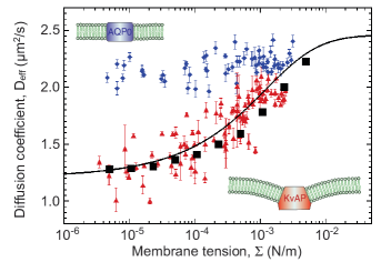
Figure 3: Figure taken from Ref. Quemeneur2014 : Protein lateral mobility in fluctuating membranes. Semi-logarithmic plot of the diffusion coefficients ($D_{\mathrm{eff}}$) as a function of the membrane tension $\Sigma$, for AQP0 ($\blacklozenge$) and KvAP ($\blacktriangle$) labeled with streptavidin QDs. KvAP data adjusted by Eq. 20 (solid line) yields a protein coupling coefficient $\Theta$ = 3.5$\times 10^{-7}$ m considering $a=5$ nm, $\kappa=20$ k_BT and $D_{0}\simeq$ 2.5 m²/s. Simulations of the protein diffusion on a membrane subject to thermal fluctuations ($\blacksquare$) agree well with the experimental data and theory. Insets: sketches of membrane deformation near proteins.

The membrane profile around the inclusion is obtained by the same method. The lateral characteristic width of this profile is the cross-over length between the tension and the bending regime for the fluctuations, namely $\xi=\sqrt{\kappa/\Sigma}$, while the characteristic height of the membrane deformation at zero tension scales as $\Theta$. The geometry of the local deformation from the membrane mid-plane induced by KvAP when subjected to various tensions is shown in Fig. 4. Using the method of Naji2007 ; Naji2009 ; Sigurdsson2013 , we have carried out simulations, which also confirm the expected theoretical membrane profile as shown in Fig. 4.

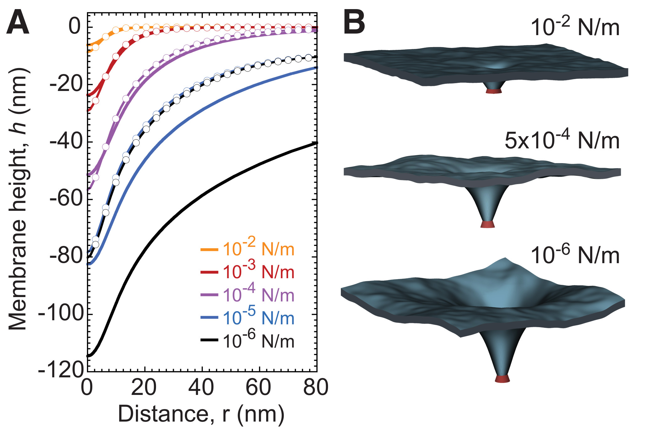
Figure 4: Figure taken from Ref. Quemeneur2014 : Membrane shape as a function of the tension. (A) Theoretical profile with parameters $\Theta=3.5\times 10^{-7}$m, $\kappa$ = 20 k_BT, $a_{\mathrm{p}}$ = 4 nm (solid lines). Profile calculated from the numerical energy minimum shape using simulation (dashed line). The height value far away from the inclusion is chosen to be zero. Discrepancy at low tension originates from the finite size of the membrane $L^{2}$ used in the simulations (see SI). (B) Three-dimensional membrane profiles obtained from numerical simulations for three different tensions.

Discussion of the results of the polaron model

We find that theory and simulations fit very well the experimental results for the diffusion coefficient of KvAP using a coupling coefficient $\Theta=3.5\times 10^{-7}$ m. This proves that the mechanical coupling between the proteins and the membrane can strongly affect protein mobility. At high tension, the experimental data of AQP0 and KvAP converge to the same plateau value, consistently with the SD limit since they have about the same steric radius. As a control, the diffusion coefficient of pure lipids was measured and found to be independent of tension as for AQP0. The corresponding constant value for $D_{0}$ agrees with the prediction of the SD model, using a lipid size $a_{\mathrm{p}}=0.5$ nm. At lower tension, Fig. 3 shows that the KvAP data starts to deviate significantly from the plateau at $\Sigma\sim 5\times 10^{-3}$ N/m, which corresponds to the point at which the lateral characteristic length $\xi$ is of the order of the protein size.

An additional outcome of this approach concerns the dependence of $D_{\mathrm{eff}}$ with the protein radius $a_{\mathrm{p}}$, which can be obtained from the following scaling argument. Since the protein makes a fixed angle with respect to the membrane, $C_{p}\sim 1/a_{\mathrm{p}}$. Given the relation $\Theta=4\pi a_{p}^{2}C_{p}$, this implies $\Theta\sim a_{\mathrm{p}}$. Below the cross-over to the SD regime, the local membrane deformation is much larger than the protein size $a_{\mathrm{p}}\ll\xi$, and the drag is dominated by the contribution due to the membrane deformation. Therefore using Eq. 20, one finds $D_{\mathrm{eff}}\sim k_{B}Ta/a_{\mathrm{p}}^{2}$, in agreement with Ref. Demery2010 . Note that such a result is also compatible with the Stokes-Einstein scaling law in $1/a_{\mathrm{p}}$ obtained in Ref. Naji2007 , because in this reference only one characteristic length for the protein is used thus $a\simeq a_{\mathrm{p}}$.

Despite a good agreement between model and data, the physical interpretation of the coupling coefficient $\Theta$ requires a more detailed discussion. Indeed, the spontaneous curvature deduced from this coupling coefficient via a fit of the data is significantly larger than that obtained from thermodynamic measurements, based on the preferential sorting at equilibrium of the proteins between GUV and highly curved membrane nanotubes Aimon2014 . One possible interpretation for this discrepancy is that in dynamic measurements, the basic relevant object, namely the association of the moving protein with the deformed membrane around it, may have a size larger than $a_{\mathrm{p}}$. Such an enhancement of the size could in principle describe physically a layer of lipids dragged by the motion of the protein as considered in Camley2012 . However, given the value of the coupling coefficient $\Theta$, this translates into an effective radius of 47 nm, a rather large value with respect to the lipid and protein sizes (0.5 and 4 nm respectively). For this reason, we have proposed in Ref. Quemeneur2014 an alternate explanation, namely that this discrepancy reflects an additional source of internal dissipation, which for the present problem, could arise from inter-monolayer slip due to the motion of the inclusion. By considering this additional dissipative mechanism internal to the membrane, we have shown that we can still account for the dependence of $D_{\mathrm{eff}}$ versus $\Sigma$, but with a lower a coupling coefficient $\Theta=3.4\times 10^{-8}$ m, corresponding to a $C_{p}$ = 0.16 nm^-1. This value is then much more compatible with the thermodynamic measurements previously reported in Aimon2014 .

5.4 Application to other order parameters

An important advantage of the polaron model is that it can be applied to other order parameters than the membrane height. Already in the previous subsection, we have mentioned an extension of the original polaron model, including dissipation mechanisms internal to the membrane, as a possible scenario to explain the value of the coupling constant in Ref. Quemeneur2014 . In that extension, the relevant order parameter was already no longer the membrane height field, but rather the difference of lipid densities in the two leaflets of the membrane. Below, we explain how different order parameters can be described in the polaron model.

Coupling to the thickness

When the hydrophobic length of the protein differs from the membrane height, the membrane is compressed or stretched close to the protein. The order parameter $\phi(\mathbf{r})$ is the difference between the local thickness of the membrane and its average thickness. If the membrane has a bending modulus $\kappa$ and a compressibility $\chi$, the energetic operators are given by Gruner1985 ; Mouritsen1993 ; Andersen2007 :

$$\tilde{\Delta}(k) =\kappa k^{4}+\chi,$$ (21)

$$\tilde{K}(k) =\pi a_{\mathrm{p}}\Theta,$$ (22)

where the coupling constant $\Theta$ now depends on the height mismatch and the energetic cost for exposing an hydrophobic area.

To our knowledge, no dynamics has been proposed for the system. However, if we assume a simple form for the membrane friction (defined by the parameter $\gamma$ in a way which conforms to model A dynamics Chaikin1995_vol ) and if we add to that the usual hydrodynamic friction due to the flow created in the solvent, we can propose an operator of the form

$$\tilde{R}(k)=\gamma+\frac{1}{4\eta k}.$$ (23)

Coupling to the composition

Real membranes are composed of several types of lipids, which may be mixed or separated. Proteins may couple to the composition field if they are preferentially wetted by one kind of lipids. Close to the demixing transition, which can be controlled in vitro in lipid vesicles Veatch2003 ; Veatch2007 , this coupling to the composition induces long-range forces between the proteins Machta2012 . Numerical simulations have shown that it may induce the aggregation of proteins Reynwar2008 .

In the simplest case, the relevant order parameter $\phi(\mathbf{r})$ is the difference between the local and average concentrations of a lipid specie. Its energy involves its correlation length, $\xi$, which diverges at the demixing transition, allowing long-range forces. The dynamics is conserved, the timescale being set by the diffusion coefficient $D_{0}$ of the lipids. The operators take the form Taniguchi1996

$$\tilde{\Delta}(k) =A\left[k^{2}+\xi^{-2}\right],$$ (24)

$$\tilde{K}(k) =\Theta,$$ (25)

$$\tilde{R}(k) =D_{0}k^{2},$$ (26)

where $\Theta$ quantifies again the strength of the coupling. Similarly to what happens for the interaction between proteins, the strongest effect on the mobility is expected close to the demixing transition (see also Ref. Fujitani2013 for a careful calculation of the drag coefficient of a diffusing domain in a near critical binary mixture).

In the description given above, we have not included the fact that the different lipid species may have different spontaneous curvatures. If this is the case Taniguchi1996 ; Yanagisawa2007 , the concentration field is coupled to the curvature field and there are two order parameters.

Coupling to other fields

The membrane could be coupled to other order parameters, and to several parameters at the same time. This situation has been evoked in the previous section, where the curvature is coupled to the composition. Also, a coupling of the membrane curvature to the lipid density in the two leaflets has been suggested to provide another dissipative mechanism in Ref. Quemeneur2014 . The polaron model needs to be extended to deal with these situations where there are several order parameters.

Another possible order parameter is the liquid crystalline order parameter of the lipids, which is expected to be distorted near small inclusions like proteins Bartolo2000 . The dynamics of a liquid crystalline order parameter can be described using continuum theories of liquid crystals and there are many studies on the dynamics of topological defects in liquid crystals Chaikin1995_vol ; Gennes1993 . Pre-transition (or pre-melting) effects which are well known in liquid crystals are also relevant for transmembrane proteins, which can for instance stabilize a microscopic order–disorder interface, when their hydrophobic thickness matches that of the disordered phase and when they are embedded in an ordered bilayer Katira2016 .

It is important to appreciate that if the protein couples to the membrane through an order parameter different from the height field, like a concentration field or a nematic order parameter field, it could happen that there will be no observable membrane deformation near the protein, while the order parameter is still perturbed.

5.5 Extension of the polaron model

We discuss here three ways to extend the simple polaron model presented in Sec. 5.2. First, we consider the case where several order parameters are coupled together and with the protein. Second, we discuss different ways to couple the order parameter and the protein. Finally, the coupling of the dynamics of the order parameter to the hydrodynamic flow in the membrane is evoked.

Coupling to several order parameters

There are cases where several order parameters $\phi_{\alpha}(\mathbf{r})$ are coupled Taniguchi1996 ; Quemeneur2014 . The polaron model can be extended to handle several order parameters. The three operators become matrix operators:

$$\Delta(\mathbf{r}) \rightarrow\Delta_{\alpha\beta}(\mathbf{r}),$$ (27)

$$K(\mathbf{r}) \rightarrow K_{\alpha}(\mathbf{r}),$$ (28)

$$R(\mathbf{r}) \rightarrow R_{\alpha\beta}(\mathbf{r}).$$ (29)

In this way, the new hamiltonian becomes

$$\mathcal{H}[\phi(\mathbf{r}),\mathbf{R}]=\frac{1}{2}\int\phi_{\alpha}(\mathbf{r})\Delta_{\alpha\beta}*\phi_{\beta}(\mathbf{r})d^{2}\mathbf{r}-K_{\alpha}*\phi_{\alpha}(\mathbf{R}),$$ (30)

where the greek indices run over the different order parameters and a summation over repeated indices is implicit.

The extension of the computation of the drag coefficient given in Sec. 5.2 is straightforward, leading to

$$\lambda=\frac{1}{2}\int\mathbf{k}^{2}\tilde{K}(\mathbf{k})_{\alpha}\tilde{\Delta}(\mathbf{k})^{-1}_{\alpha\beta}\tilde{R}(\mathbf{k})^{-1}_{\beta\gamma}\tilde{\Delta}(\mathbf{k})^{-1}_{\gamma\delta}\tilde{K}(\mathbf{k})_{\delta}^{*}\frac{d^{2}\mathbf{k}}{(2\pi)^{2}}.$$ (31)

Other protein couplings to the order parameter

In the example of a protein coupled to the curvature of the membrane, it is clear that a linear coupling cannot be used to “impose” a given curvature to the membrane at the location of the protein. Instead, the value of the membrane curvature depends on the Hamiltonian operators $\Delta(\mathbf{r})$ and $K(\mathbf{r})$.

The more direct way to impose the membrane curvature is to set it as a boundary condition Bitbol2010 ; Camley2012 , using a relation of the form $K*\phi(\mathbf{R})=A$ (in this case of a coupling to the membrane curvature, $A$ corresponds to the curvature of the membrane at the location of the protein, denoted $C_{p}$ above). In this framework the force can no longer be computed with Eq. 7, and one should instead integrate the stress tensor around the protein Bitbol2011 ; Capovilla2002 .

An imposed boundary condition can be modeled in the framework of the polaron model, by introducing a parameter $\alpha$ in front of the coupling operator $K(\mathbf{r})$ and tuning it so that the boundary condition is satisfied. In this case, $\alpha$ depends on the other parameters of the model (e.g., the membrane tension and bending modulus when the protein is coupled to the curvature of the membrane). This approach has been shown to give results consistent with those obtained with an imposed boundary condition Camley2012 .

Alternatively, the polaron model can be modified by replacing the linear coupling to the order parameter by a coupling of the form

$$\mathcal{H}_{\mathrm{int}}[\phi(\mathbf{r}),\mathbf{R}]=\frac{\kappa_{\mathrm{p}}}{2}\left[K*\phi(\mathbf{R})-A\right]^{2},$$ (32)

where $\kappa_{\mathrm{p}}$ is the “rigidity” of the coupling (e.g., the bending rigidity of the protein). In the limit of infinite rigidity, $\kappa_{\mathrm{p}}\to\infty$, one recovers the imposed boundary condition. This form of coupling has been used to model the coupling to curvature in Refs. Naji2009 ; Reister_Gottfried2010 . In the limit where $K*\phi(\mathbf{R})$ is small with respect to $A$, the linear coupling introduced in Eq. 4 is recovered.

In the particular case $A=0$, the coupling does not affect the average value of the order parameter, but only its fluctuations. This Casimir-like coupling gives rise to another source of drag Demery2011a and further reduction of the diffusion coefficient Demery2013 . For a coupling to curvature, when both effects (average field deformation and fluctuations) compete, the fluctuations induced part is often neglected owing to the fact that the thermal fluctuations are small, i.e. $k_{\mathrm{B}}T\ll\kappa$.

In the general case, the interaction Hamiltonian given in Eq. 32 depends on one more parameter than the linear interaction in Eq. 4. This has important implications: for example, when the coupling to membrane curvature is modeled by a linear interaction, as in Eq. 16, the rigidity of the protein and its spontaneous curvature cannot be decoupled. On the other hand the rigidity $\kappa_{\mathrm{p}}$ and the preferred average value $A$ have very different effects with the quadratic coupling, Eq. 32.

Interaction of the order parameter with the hydrodynamic flow

The polaron model is completely independent of the hydrodynamic calculation of Saffman and Delbrück, in the sense that the flow in the membrane and in the solvent are neglected, and the order parameter dynamics is not coupled to these flows. For example, if the order parameter represents the concentration difference between two lipid species, it is clear that besides diffusion, the order parameter is advected by the lipid flow in the membrane Reynwar2008 .

The coupling between the order parameter $\phi(\mathbf{r})$ and the hydrodynamic flow $\mathbf{u}(\mathbf{r})$ has been modeled by Camley and Brown Camley2012 . They found that the advection of the order significantly changes the total drag on the protein. As a result, the protein is endowed with a larger effective radius, since the lipids which are closest to the protein are carried along with it. Although this effect will affect the value of the drag, this will not change the qualitative behavior, in particular the result that the drag should scale with the particle size, in a logarithmic way in the SD regime and linearly for large particles.

Recently, another very interesting hydrodynamic model Morris2015 -Daniels2016 has been proposed to account for the experimental data on the tension dependence of the mobility of KvAP discussed in this paper and first reported in Ref. Quemeneur2014 . Assuming a negligible contribution due to the hydrodynamics of the surrounding fluid, the authors of this study have exploited a covariant formulation of the membrane hydrodynamics of the inclusion, which has specific features due to the Gaussian curvature induced locally by the inclusion. In this way, they could explain the experimental data on the mobility of KvAP without requiring additional mechanism of internal dissipation. Interestingly, a key ingredient of their model is the deformability of the inclusion, which is particularly important for gated membrane channels Morris2017 . We note that the polaron model could account for the deformability of the inclusion, and could also be combined with such hydrodynamic description of the membrane.

6 Concluding perspective

In this chapter, we have presented some simple views on the way geometrical or mechanical factors influence the mobility of membrane proteins. We have shown that one should expect generally a significant dependence of the protein mobility on its local environment.

Naturally, many molecular details affect this local environment, which makes the modeling of the protein mobility a challenging task. However, despite the complexity of this problem, there is a simple take-home message. In order to predict the way various mechanical factors affect the mobility of membrane proteins, one should not focus on the mechanical factors themselves or on the details of the local environment of the protein, but instead on the form of coupling between the membrane and the protein. We have provided in this chapter a list of various relevant couplings, and a detailed study of one coupling, namely the tension dependent coupling to the local membrane curvature. Clearly, it would be desirable to perform similar experimental studies in order to test more couplings and their dependence to other mechanical factors. The importance of these couplings goes beyond the specific question of the mobility of membrane proteins, since they are also relevant to understand the function of many membrane proteins, like voltage-gating channels, mechano-sensitive channels, G-protein coupled receptors (GPCR) or light-activated rhodopsins Phillips2009 . These couplings also play a key role in the interactions between membrane proteins, and in their self-organization into complex dynamical structures, such as membrane clusters.

At the level of single membrane proteins, other directions for future research, should investigate (i) a protein diffusing in a membrane which may be driven out of equilibrium, or (ii) a protein which can be activated or can change conformation while diffusing on the membrane. For studying the former case (i), various strategies can be used to drive a membrane out of equilibrium by applying external fields on it directly or by embedding other proteins in it on which forces can be applied Lacoste2013 . Measurements of the force dependent mobility of a membrane protein could advantageously provide information on the way it couples to its environment, which as mentioned above is a crucial aspect of the problem. For case (ii), the internal dynamics of the protein can matter for the protein mobility because different internal states can couple differently to the membrane and the characteristic time of these internal transitions (typically 10 to 1000 ms) can be much longer than the time of diffusion of the protein over a distance equal to its radius (typically < 1ms) Bouvrais2012 . For many membrane proteins, the transition rates can be tuned by changing the amount of ATP, allowing to probe different dynamical regimes for the mobility of the protein.

In cell membranes, the local environment of proteins is crowded and heterogeneous. Membrane protein crowding is of primary importance to understand the mobility of membrane proteins and membrane mediated interactions between different proteins. Such effects are not well understood and they need to be investigated more systematically both experimentally and theoretically.

We hope that this chapter can be useful to motivate further experimental and theoretical studies on these questions.

References

- (1) A. Einstein, Annalen der Physik 322, 549 (1905)
- (2) J.B. Perrin, Ann. Chim. Phys. 19, 5 (1909)
- (3) P.G. Saffman, M. Delbrück, Proc. Natl. Acad. Sci. U.S.A. 72(8), 3111 (1975)
- (4) B.D. Hughes, B.A. Pailthorpe, L.R. White, J. Fluid Mech. 110, 349 (1981)
- (5) G. Guigas, M. Weiss, Biophys. J. 95(3), L25 (2008)
- (6) E.P. Petrov, P. Schwille, Biophys. J. 94(5), L41 (2008)
- (7) E.P. Petrov, R. Petrosyan, P. Schwille, Soft Matter 8, 7552 (2012)
- (8) Y. Gambin, R. Lopez-Esparza, M. Reffay, E. Sierecki, N.S. Gov, M. Genest, R.S. Hodges, W. Urbach, Proc. Natl. Acad. Sci. U. S. A. 103, 2098 (2006)
- (9) K. Weiß, A. Neef, Q. Van, S. Kramer, I. Gregor, J. Enderlein, Biophys. J. 105(2), 455 (2013)
- (10) S. Ramadurai, A. Holt, V. Krasnikov, G. van den Bogaart, J.A. Killian, B. Poolman, J. Am. Chem. Soc. 131(35), 12650 (2009)
- (11) F. Quemeneur, J.K. Sigurdsson, M. Renner, P.J. Atzberger, P. Bassereau, D. Lacoste, Proc. Natl. Acad. Sci. U.S.A. 111(14), 5083 (2014)
- (12) Y. Gambin, M. Reffay, E. Sierecki, F. Homblé, R.S. Hodges, N.S. Gov, N. Taulier, W. Urbach, J. Phys. Chem. B 114(10), 3559 (2010)
- (13) Y.A. Domanov, S. Aimon, G.E.S. Toombes, M. Renner, F. Quemeneur, A. Triller, M.S. Turner, P. Bassereau, Proc. Natl. Acad. Sci. U. S. A. 108(31), 12605 (2011)
- (14) D.R. Daniels, M.S. Turner, Langmuir 23(12), 6667 (2007)
- (15) T.T. Hormel, S.Q. Kurihara, M.K. Brennan, M.C. Wozniak, R. Parthasarathy, Phys. Rev. Lett. 112, 188101 (2014)
- (16) S. Aimon, A. Callan-Jones, A. Berthaud, M. Pinot, G.E.S. Toombes, P. Bassereau, Dev. Cell 28(2), 212 (2014)
- (17) G. Chang, R.H. Spencer, A.T. Lee, M.T. Barclay, D.C. Rees, Science 282(5397), 2220 (1998)
- (18) Z. Liu, C.S. Gandhi, D.C. Rees, Nature 461(7260), 120 (2009)
- (19) B.A. Camley, F.L.H. Brown, Soft Matter 9(19), 4767 (2013)
- (20) K. Seki, S. Ramachandran, S. Komura, Phys. Rev. E 84, 021905 (2011)
- (21) H.A. Stone, A. Ajdari, J. Fluid Mech 369, 151 (1998)
- (22) M. Goulian, R. Bruinsma, P. Pincus, EPL (Europhysics Letters) 22(2), 145 (1993)
- (23) B. Reynwar, M. Deserno, Biointerphases 3(2), FA117 (2008)
- (24) E. Reister, U. Seifert, Europhys. Lett. 71(5), 859 (2005)
- (25) B.J. Reynwar, G. Illya, V.A. Harmandaris, M.M. Muller, K. Kremer, M. Deserno, Nature 447(7143), 461 (2007)
- (26) A. Naji, P.J. Atzberger, F.L.H. Brown, Phys. Rev. Lett. 102(13), 138102 (2009)
- (27) O.S. Andersen, R.E. Koeppe, Annu. Rev. Biophys. Biomol. Struct. 36(1), 107 (2007)
- (28) M. Winterhalter, W. Helfrich, Phys. Rev. A 36, 5874 (1987)
- (29) R. Phillips, T. Ursell, P. Wiggins, P. Sens, Nature 459(7245), 379 (2009)
- (30) E. Reister-Gottfried, S.M. Leitenberger, U. Seifert, Phys. Rev. E 75(1), 011908 (2007)
- (31) A. Naji, A.J. Levine, P.A. Pincus, Biophys. J. 93(11), L49 (2007)
- (32) L.D. Landau, Phys. Z. Sowjetunion 3, 644 (1933)
- (33) V. Démery, D.S. Dean, Phys. Rev. Lett. 104(8), 080601 (2010)
- (34) V. Démery, D.S. Dean, European Physical Journal E 32, 377 (2010)
- (35) P.M. Chaikin, T.C. Lubensky, Principles of condensed matter physics (Cambridge University Press, 1995)
- (36) D.S. Dean, V. Démery, J. Phys.: Condens. Matter 23(23), 234114 (2011)
- (37) V. Démery, D.S. Dean, Phys. Rev. E 84(1), 011148 (2011)
- (38) S.M. Leitenberger, E. Reister-Gottfried, U. Seifert, Langmuir 24, 1254 (2008)
- (39) E. Reister-Gottfried, S.M. Leitenberger, U. Seifert, Phys. Rev. E 81, 031903 (2010)
- (40) J.K. Sigurdsson, F.L. Brown, P.J. Atzberger, Journal of Computational Physics 252(0), 65 (2013)
- (41) B. Camley, F. Brown, Phys. Rev. E 85(6), 061921 (2012)
- (42) S.M. Gruner, Proc. Natl. Acad. Sci. U.S.A. 82(11), 3665 (1985)
- (43) O.G. Mouritsen, M. Bloom, Annu. Rev. Biophys. Biomol. Struct. 22(1), 145 (1993). PMID: 8347987
- (44) S.L. Veatch, S.L. Keller, Biophys. J. 85(5), 3074 (2003)
- (45) S.L. Veatch, O. Soubias, S.L. Keller, K. Gawrisch, Proc. Natl. Acad. Sci. U.S.A. 104(45), 17650 (2007)
- (46) B.B. Machta, S.L. Veatch, J.P. Sethna, Phys. Rev. Lett. 109(13), 138101 (2012)
- (47) T. Taniguchi, Phys. Rev. Lett. 76(23), 4444 (1996)
- (48) Y. Fujitani, J. Phys. Soc. Jpn. 82(12), 124601 (2013)
- (49) M. Yanagisawa, M. Imai, T. Masui, S. Komura, T. Ohta, Biophysical Journal 92(1), 115 (2007)
- (50) D. Bartolo, D. Long, J.B. Fournier, Europhys. Lett. 49(6), 729 (2000)
- (51) P.G. de Gennes, J. Prost, The physics of liquid crystals (Oxford University Press, 1993)
- (52) S. Katira, K.K. Mandadapu, S. Vaikuntanathan, B. Smit, D. Chandler, eLife 5, e13150 (2016)
- (53) A.F. Bitbol, P.G. Dommersnes, J.B. Fournier, Phys. Rev. E 81(5), 050903 (2010)
- (54) A.F. Bitbol, J.B. Fournier, Physical Review E 83(6), 061107 (2011)
- (55) R. Capovilla, J. Guven, J. Phys. A: Math. and Gen. 35, 6233 (2002)
- (56) V. Démery, D.S. Dean, Phys. Rev. E 84(1), 010103 (2011)
- (57) V. Démery, Phys. Rev. E 87(5), 052105 (2013)
- (58) R.G. Morris, M.S. Turner, Phys. Rev. Lett. 115, 198101 (2015)
- (59) D.R. Daniels, The European Physical Journal E 39(10), 96 (2016)
- (60) R.G. Morris, Biophys. J. 112(1), 3 (2017)
- (61) D. Lacoste, P. Bassereau, in Liposomes, Lipid Bilayers and Model Membranes: From Basic Research to Applications, ed. by G. Pabst (Taylor and Francis, 2013), pp. 271–287
- (62) Bouvrais, H. and Cornelius, F., and Ipsen, J. H. and Mouritsen, O., Proc. Natl. Acad. Sci. U.S.A. 109(45), 18442 (2012)