Linear Receivers in Non-stationary Massive MIMO Channels with Visibility Regions

Abstract

In a massive MIMO system with large arrays, the channel becomes spatially non-stationary. We study the impact of spatial non-stationarity characterized by visibility regions (VRs) where the channel energy is significant on a portion of the array. Relying on a channel model based on VRs, we provide expressions of the signal-to-interference-plus-noise ratio (SINR) of conjugate beamforming (CB) and zero-forcing (ZF) precoders. We also provide an approximate deterministic equivalent of the SINR of ZF precoders. We identify favorable and unfavorable multi-user configurations of the VRs and compare the performance of both stationary and non-stationary channels through analysis and numerical simulations.

I Introduction

A massive MIMO system [1] is characterized by the use of many antennas and support for multiple users. At the extreme, the arrays may be physically very large [2, 3, 4] and integrated into large structures like stadiums, or shopping malls. Unfortunately, when the dimension of the antenna array becomes large, different kinds of non-stationarities appear across the array. Further, different parts of the array may observe the same channel paths with different power, or even entirely different channel paths [2]. This effect may even be observed for compact arrays [2]. We show that non-stationarity in massive arrays has a significant impact on performance assessment and transceiver design.

We propose a simple non-stationary channel model and analyze the performance of CB and ZF in the downlink of a multi-user massive MIMO system. The channel model is based on VRs that capture the received power variation across the array. We also propose a closed-form approximation of the SINR of the ZF receiver. The expression shows the dependence of the SINR on channel parameters and allows a comparison between spatially stationary and non-stationary channels. The analysis and simulation results show that the impact of spatial non-stationarity on the performance of linear receivers is scenario dependent.

Few theoretical studies exist on spatially non-stationary channels in massive MIMO systems. In [5] a spherical wave-front based LOS channel model was proposed and the channel capacity is studied with the proposed model. In [6] an upper bound on the ergodic capacity of a non-stationary channel was provided. No prior work, however, has studied the performance of linear precoders with non-stationary channels.

Notation: ${\mathbf{X}}$ is a matrix, ${\mathbf{x}}$ is a vector, $\mathcal{X}$ is a set, $x$ and $X$ are scalars. Superscript ${\sf T}$, and $\ast$, represent transpose, and conjugate transpose, respectively. ${\mathbb{E}}[\cdot]$ is the expectation, and $\mathcal{C}\mathcal{N}({\mathbf{x}},{\mathbf{X}})$ is a complex Normal with mean ${\mathbf{x}}$ and covariance ${\mathbf{X}}$. The identity matrix is ${\mathbf{I}}$ and $\|{\mathbf{x}}\|_{p}$ is the $p$-norm. The cardinality of a set $\mathcal{X}$ is $|\mathcal{X}|$. The matrix ${\mathbf{X}}={\rm diag}({\mathbf{x}})$ is a diagonal matrix with the vector ${\mathbf{x}}$ on its main diagonal, and ${\rm tr}({\mathbf{X}})$ is the trace of matrix ${\mathbf{X}}$. The operator $\overset{\rm{a.s.}}{\rightarrow}$ denotes almost sure convergence.

II System and channel model

We consider a narrowband broadcast system where the base-station (BS) equipped with $M$ antennas is serving $K$ single-antenna users ($M\geq K$). The BS serves all the users using the same time-frequency resource. The signal for user $k$, $s_{k}$ is precoded by ${\mathbf{g}}_{k}\in{\mathbb{C}}^{M}$ and scaled by the signal power $p_{k}\geq 0$ before transmission. The transmit vector ${\mathbf{x}}$ is the linear combination of the precoded and scaled signals of all the users, i.e.,

$${\mathbf{x}}=\sum_{k=1}^{K}\sqrt{p_{k}}{\mathbf{g}}_{k}s_{k}.$$ (1)

Let ${\mathbf{G}}=[{\mathbf{g}}_{1},{\mathbf{g}}_{2},\cdots,{\mathbf{g}}_{K}]\in{\mathbb{C}}^{M\times K}$ be the combined precoding matrix, ${\mathbf{P}}={\rm diag}([p_{1},p_{2},\cdots,p_{K}]^{\sf T})\in{\mathbb{R}}^{K\times K}$ be the diagonal matrix of signal powers, and $P\geq 0$ be the total power. The combined precoding matrix ${\mathbf{G}}$ is normalized to satisfy the power constraint

$${\mathbb{E}}[\|{\mathbf{x}}\|^{2}]={\rm tr}({\mathbf{P}}{\mathbf{G}}^{\ast}{\mathbf{G}})=P.$$ (2)

Let ${\mathbf{h}}_{k}\in{\mathbb{C}}^{M}$ denotes the random channel from the BS to user $k$. Then the received signal at the user $k$ is

$${\mathbf{y}}_{k}={\mathbf{h}}_{k}^{\ast}{\mathbf{x}}+n_{k},\leavevmode\nobreak\ k=1,2,\cdots,K,$$ (3)

where $n_{k}\sim\mathcal{C}\mathcal{N}({\mathbf{0}},\sigma^{2})$ is the additive noise. Assuming independent Gaussian signaling, i.e., $s_{k}\sim\mathcal{C}\mathcal{N}(0,1)$ and ${\mathbb{E}}[s_{i}s_{j}^{\ast}]=0,\leavevmode\nobreak\ i\neq j$, the SINR $\gamma_{k}$ of user $k$ can be written as

$$\gamma_{k}=\frac{p_{k}|{\mathbf{h}}_{k}^{\ast}{\mathbf{g}}_{k}|^{2}}{\sum\limits_{j=1,j\neq k}^{K}p_{j}|{\mathbf{h}}_{k}^{\ast}{\mathbf{g}}_{j}|^{2}+\sigma^{2}}.$$ (4)

Let ${\mathbf{H}}=[{\mathbf{h}}_{1}\leavevmode\nobreak\ {\mathbf{h}}_{2}\leavevmode\nobreak\ \cdots\leavevmode\nobreak\ {\mathbf{h}}_{K}]\in{\mathbb{C}}^{M\times K}$ denote the channel matrix between the BS and $K$ users. Then, the CB precoder is

$${\mathbf{G}}_{{{\mathrm{C}}{\mathrm{B}}}}=\beta_{{\mathrm{C}}{\mathrm{B}}}{\mathbf{H}},$$ (5)

and the ZF precoder is

$${\mathbf{G}}_{{{\mathrm{Z}}{\mathrm{F}}}}=\beta_{{\mathrm{Z}}{\mathrm{F}}}{\mathbf{H}}({\mathbf{H}}^{\ast}{\mathbf{H}})^{-1},$$ (6)

where the scaling factors $\beta_{{\mathrm{C}}{\mathrm{B}}}=\sqrt{P/{\rm tr}({\mathbf{P}}{\mathbf{H}}^{\ast}{\mathbf{H}})}$ and $\beta_{{\mathrm{Z}}{\mathrm{F}}}=\sqrt{P/{\rm tr}({\mathbf{P}}({\mathbf{H}}^{\ast}{\mathbf{H}})^{-1})}$ ensure that the power constraint (2) is met.

By defining $\rho=P/\sigma^{2}$ as the signal-to-noise ratio (SNR) and using (5) in (4), the SINR of the $k$th user for CB is

$$\gamma_{k}^{({{\mathrm{C}}{\mathrm{B}}})}=p_{k}\frac{\rho|{\mathbf{h}}_{k}^{\ast}{\mathbf{h}}_{k}|^{2}}{\rho\sum\limits_{j=1,j\neq k}^{K}p_{j}|{\mathbf{h}}_{k}^{\ast}{\mathbf{h}}_{j}|^{2}+{\rm tr}({\mathbf{P}}{\mathbf{H}}^{\ast}{\mathbf{H}})}.$$ (7)

Similarly, using (6) in (4), the SINR of the $k$th user for ZF is

$$\gamma_{k}^{({{\mathrm{Z}}{\mathrm{F}}})}=p_{k}\frac{\rho}{{\rm tr}({\mathbf{P}}({\mathbf{H}}^{\ast}{\mathbf{H}})^{-1})}.$$ (8)

Let ${\mathbf{R}}_{k}\in{\mathbb{C}}^{M\times M}$ be the spatial correlation matrix of user $k$ corresponding to the case of a stationary channel. Further, let ${\mathbf{D}}_{k}$ be a diagonal matrix such that if the signal transmitted from only $D_{k}$ antennas is received by the user $k$, ${\mathbf{D}}_{k}$ has $D_{k}$ non-zero diagonal entries. This diagonal matrix ${\mathbf{D}}_{k}$ models the VR of user $k$. For the proposed channel model, we introduce a matrix $\boldsymbol{\Theta}_{k}$ of the form

$$\boldsymbol{\Theta}_{k}={\mathbf{D}}_{k}^{\frac{1}{2}}{\mathbf{R}}_{k}{\mathbf{D}}_{k}^{\frac{1}{2}}.$$ (9)

If ${\mathbf{z}}_{k}\sim\mathcal{C}\mathcal{N}(0,\frac{1}{M}{\mathbf{I}})$, then by the proposed model, the channel of user $k$, ${\mathbf{h}}_{k}$ is

$${\mathbf{h}}_{k}=\sqrt{M}\boldsymbol{\Theta}_{k}^{\frac{1}{2}}{\mathbf{z}}_{k}.$$ (10)

For stationary channel ${\mathbf{D}}_{k}={\mathbf{I}}$, and $\boldsymbol{\Theta}_{k}={\mathbf{R}}_{k}$. Therefore, the channel model (10) subsumes the well known correlated channel studied in [7, 8].

III Large system analysis in stationary channels

Correlated stationary channels (i.e., $\boldsymbol{\Theta}_{k}={\mathbf{R}}_{k}$) were studied in [7, 8], under the following assumptions.

1. $M,K,\frac{M}{K}\rightarrow\infty$. (BS equipped with a large number of antennas serving a large number of users.)

2. The covariance matrices have a uniformly bounded spectral norm i.e., $\underset{M,K\rightarrow\infty}{\lim\sup}\underset{1\leq k\leq K}{\sup}\|{\mathbf{R}}_{k}\|=\mathcal{O}(1)$ [9]. (User channels are not highly correlated.)

3. The power $p_{\rm{max}}=\max(p_{1},p_{2},\cdots,p_{K})$ is of the order $O(1/K)$, i.e., $\|{\mathbf{P}}\|=O(1/K)$. (Transmission power for all the users is on the same order.)

With A1-A3, the deterministic equivalent of $\gamma_{k}^{({{\mathrm{C}}{\mathrm{B}}})}$ can be written as [7, eq. 24]

$$\bar{\gamma}_{k}^{({{\mathrm{C}}{\mathrm{B}}})}=p_{k}\frac{\rho({\rm tr}({\mathbf{R}}_{k})^{2})}{\rho\sum\limits_{j=1,j\neq k}^{K}p_{j}{\rm tr}({\mathbf{R}}_{k}{\mathbf{R}}_{j})+\sum\limits_{j=1}^{K}p_{j}{\rm tr}({\mathbf{R}}_{j})}.$$ (11)

where $\gamma_{k}^{({{\mathrm{C}}{\mathrm{B}}})}-\bar{\gamma}_{k}^{({{\mathrm{C}}{\mathrm{B}}})}\overset{\rm{a.s.}}{\underset{M\rightarrow\infty}{\longrightarrow}}0$. Using A1-A3 and some additional assumptions, the deterministic equivalent of $\gamma_{k}^{({{\mathrm{Z}}{\mathrm{F}}})}$ was obtained in [8, eq. 34]. That expression, though, is not closed form and as such is not suitable for comparing stationary and non-stationary channels. With this motivation, we provide a closed form approximate expression in the following theorem.

Theorem 1.

Under the assumptions A1-A3, an approximate deterministic equivalent of $\gamma_{k}^{({{\mathrm{Z}}{\mathrm{F}}})}$ in (8) is

$${\bar{\gamma}}_{k}^{({{\mathrm{Z}}{\mathrm{F}}})}=p_{k}\frac{\rho}{\sum\limits_{i=1}^{K}p_{i}\big{(}{\rm tr}({\mathbf{R}}_{i})-\sum\limits_{j=1,j\neq i}^{K}\frac{{\rm tr}({\mathbf{R}}_{i}{\mathbf{R}}_{j})}{{\rm tr}({\mathbf{R}}_{j})}\big{)}^{-1}},$$ (12)

which is guaranteed to be non-negative as $\frac{M}{K}\rightarrow\infty$.

Proof.

See Appendix A. ∎

Remark: The expression (12) is obtained with the help of a diagonal approximation (see Appendix A). In the following proposition, we provide the order of absolute error in this approximation.

Proposition 1.

The error in approximating the $O(K)$ term ${\mathbf{h}}_{i}^{\ast}\bar{\mathbf{H}}_{i}(\bar{\mathbf{H}}_{i}^{\ast}\bar{\mathbf{H}}_{i})^{-1}\bar{\mathbf{H}}_{i}^{\ast}{\mathbf{h}}_{i}$ by ${\mathbf{h}}_{i}^{\ast}\bar{\mathbf{H}}_{i}{\mathbf{V}}^{-1}\bar{\mathbf{H}}_{i}^{\ast}{\mathbf{h}}_{i}$ (where ${\mathbf{V}}$ is defined in (21)), is

$$\epsilon_{i}=|{\mathbf{h}}_{i}^{\ast}\bar{\mathbf{H}}_{i}(\bar{\mathbf{H}}_{i}^{\ast}\bar{\mathbf{H}}_{i})^{-1}\bar{\mathbf{H}}_{i}^{\ast}{\mathbf{h}}_{i}-{\mathbf{h}}_{i}^{\ast}\bar{\mathbf{H}}_{i}{\mathbf{V}}^{-1}\bar{\mathbf{H}}_{i}^{\ast}{\mathbf{h}}_{i}|,$$ (13)

and is of $O\left(\frac{K}{\sqrt{M}}\right)$.

Proof.

See Appendix B. ∎

IV Stationary versus non-stationarity channels

For non-stationary channels, we introduce two additional assumptions.

1. $D_{k}\rightarrow\infty,\leavevmode\nobreak\ \forall k.$ (Large VR for each user).

2. $\underset{M,K\rightarrow\infty}{\lim\sup}\underset{1\leq k\leq K}{\sup}\|\boldsymbol{\Theta}_{k}\|<\infty$. (Non-stationary user channels are not highly correlated.)

With this, the same analysis that led to (11) and (12) can be used for non-stationary channels. In fact, only ${\mathbf{R}}$ needs to be replaced with $\boldsymbol{\Theta}$ in theoretical expressions (11), and (12) to get the results for the non-stationary case.

For comparison between stationary and non-stationary channels, we make a few simplistic choices of system and channel parameters. Specifically, we start by considering $p_{k}=\frac{P}{K}\leavevmode\nobreak\ \forall k$ and ${\mathbf{R}}_{k}={\mathbf{I}}\leavevmode\nobreak\ \forall k$. For non-stationary channels, we consider two types of channel normalization.

Normalization 1, ${\rm tr}(\boldsymbol{\Theta}_{k})={\rm tr}({\mathbf{R}}_{k})=M,\leavevmode\nobreak\ \forall k$: This ensures that the stationary and non-stationary channels have the same norm. The physical implication of normalization 1 is shown in Fig. 1 (a). User terminal 1 (i.e., farther) receives signal from all antennas but with lower power, whereas user terminal 2 (i.e., closer) receives signal from fewer antennas but with higher power. This is achieved by choosing ${\mathbf{D}}_{k}={\rm diag}([{\mathbf{0}},\sqrt{\frac{M}{D_{k}}}{\mathbf{1}}_{D_{k}},{\mathbf{0}}]^{\sf T})$.

Normalization 2, ${\rm tr}(\boldsymbol{\Theta}_{k})=D_{k}\leavevmode\nobreak\ \forall k$: The physical implication of normalization 2 is shown in Fig. 1 (b). User terminal $1$ and $2$ are equidistant from the BS, however, user terminal $2$ receives signal from only a few antennas. This is achieved by choosing ${\mathbf{D}}_{k}={\rm diag}([{\mathbf{0}},{\mathbf{1}}_{D_{k}},{\mathbf{0}}]^{\sf T})$.

To further simplify the comparison, we assume that $D_{k}=D\leavevmode\nobreak\ \forall k$.

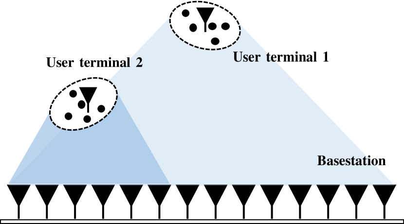
(a) Physical implication of normalization 1 i.e., ${\rm tr}(\boldsymbol{\Theta})=M$.

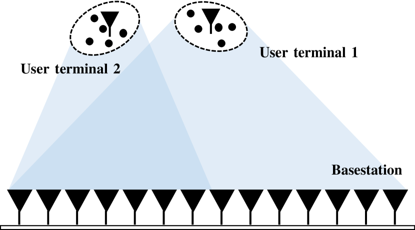
(b) Physical implication of normalization 2 i.e., ${\rm tr}(\boldsymbol{\Theta})=D$.

Figure 1: Physical implication of normalization 1 (i.e., ${\rm tr}(\boldsymbol{\Theta})=M$) and normalization 2 (i.e., ${\rm tr}(\boldsymbol{\Theta})=D$).

We outline the SINR for CB in stationary and non-stationary channels with normalization 1 in detail below. The derivations for normalization 2 and ZF precoding are similar and the results are summarized in Table  I.

The SINR of CB (11) for stationary channels simplifies to

$$\gamma_{k}^{({{\mathrm{C}}{\mathrm{B}}})}-{\rm{st.}}=\frac{\rho M}{\rho(K-1)+K}.$$ (14)

For the non-stationary channel under consideration, a user receives the signal transmitted from $D$ antennas. The indices of these antennas for user $k$ are collected in a set $\mathcal{D}_{k}$. The SINR of user $k$ depends on $|\mathcal{D}_{k}\cap\mathcal{D}_{j}|\leavevmode\nobreak\ \forall j\neq k$ (i.e., inter-user interference). For example, if $K=2$, $D=M/2$ and $\mathcal{D}_{1}=\mathcal{D}_{2}=\{1,\cdots,M/2\}$, then $|\mathcal{D}_{1}\cap\mathcal{D}_{2}|=D$ and there is high inter-user interference. If, however, $\mathcal{D}_{1}=\{1,\cdots,M/2\}$ and $\mathcal{D}_{2}=\{M/2+1,\cdots,M\}$, then $|\mathcal{D}_{1}\cap\mathcal{D}_{2}|=0$ and there is no inter-user interference. Thus for non-stationary channels, we consider the best-case (and worst-case) index sets $\mathcal{D}_{k}$ that result in maximum (and minimum) possible SINR for the considered setup.

In the worst-case, there is high inter-user interference. This happens, when all the $K$ users receive the signal from the same $D$ antenna elements. In this case, assuming ${\rm tr}(\boldsymbol{\Theta})=M$, it can be shown that

$$\gamma_{k}^{({{\mathrm{C}}{\mathrm{B}}})}-{\rm{non\leavevmode\nobreak\ st.\leavevmode\nobreak\ (worst)}}=\frac{\rho M}{\rho\frac{M}{D}(K-1)+K}.$$ (15)

There is an additional factor $M/D$ in the first term in denominator of (15) compared to (14). Therefore, for worst-case, the smaller the VR of the user (i.e., in this case, the number of active antennas $D$), the more SINR loss for non-stationary channels.

In the best-case, there is low inter-user interference for all the $K$ users. The best-case antenna indices can be found using counting arguments. Asymptotically, with a user $k$ receiving signal from $D$ antennas, and a total of $M$ antennas, we can arrange only $M/D$ users without any inter-user interference. If we continue this arrangement for all users, there will be $\frac{KD}{M}-1$ interfering users for any user $k$. With this observation, the best-case SINR can be written as

$$\gamma_{k}^{({{\mathrm{C}}{\mathrm{B}}})}-{\rm{non\leavevmode\nobreak\ st.\leavevmode\nobreak\ (best)}}=\frac{\rho M}{\rho(K-\frac{M}{D})+K}.$$ (16)

If $KD\leq M$, there will be no inter-user interference with the arrangement described above and (16) can be further simplified. Note that the first term in the denominator of (14) and (16) differs. Specifically, for best-case, if $\frac{M}{D}$ is large (i.e., smaller VR), then the SINR of CB precoders for non-stationary channels can be better than the stationary channels.

Table I: SINR expressions for CB and ZF precoders for stationary and non-stationary channels.

	Stationary	Non-stationary
			Worst	Best
CB	$\frac{\rho M}{\rho(K-1)+K}$	Normalization 1: ${\rm tr}(\boldsymbol{\Theta}_{k})=M$	$\frac{\rho M}{\rho\frac{M}{D}(K-1)+K}$	$\frac{\rho M}{\rho(K-\frac{M}{D})+K}$
		Normalization 2: ${\rm tr}(\boldsymbol{\Theta}_{k})=D$	$\frac{\rho D}{\rho(K-1)+K}$	$\frac{\rho D}{\rho(\frac{KD}{M}-1)+K}$
ZF	$\frac{\rho(M-K+1)}{K}$	Normalization 1: ${\rm tr}(\boldsymbol{\Theta}_{k})=M$	$\frac{\rho(M-\frac{M}{D}(K-1))}{K}$	$\frac{\rho(M-K+\frac{M}{D})}{K}$
		Normalization 2: ${\rm tr}(\boldsymbol{\Theta}_{k})=D$	$\frac{\rho(D-K+1)}{K}$	$\frac{\rho(D-\frac{KD}{M}+1)}{K}$

V Numerical results

We verify the analysis of the non-stationary channels. We consider $M=60$, $K=M/2$, and $\rho=$10\text{\,}\mathrm{dB}$$. We plot the SINR results against the active number of antennas per user $D$. We consider both the best-case and worst-case antenna configurations discussed in Section IV. We plot the results for normalization 1 i.e., ${\rm tr}(\boldsymbol{\Theta})=M$ in Fig. 2(a), and for normalization 2 i.e., ${\rm tr}(\boldsymbol{\Theta})=D$ in Fig. 2(b). From Fig. 2(a), notice that when $D$ is small, the SINR of the non-stationary channels in the best-case (worst-case) is higher (lower) than the stationary channels. The worst-case performance loss for CB (ZF) is as high as $15\text{\,}\mathrm{dB}$ ($12.5\text{\,}\mathrm{dB}$). As $D$ increases, however, the SINR in the non-stationary channels converge to the SINR of the stationary channels. This observation holds for both CB and ZF precoding. The ZF curve in the worst-case starts from $D=30$. For smaller values of $D$, the channel matrix ${\mathbf{H}}$ is rank deficient and ZF precoding fails. From Fig. 2(b), we notice that with normalization $2$, the SINR of the non-stationary channels is lower than the SINR of the stationary channels (for $\rho=$10\text{\,}\mathrm{dB}$$). With normalization 2, the performance loss for both CB and ZF can be as high as $15\text{\,}\mathrm{dB}$.

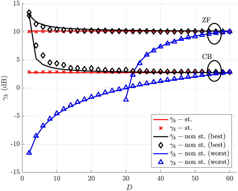
(a) Normalization 1: ${\rm tr}(\boldsymbol{\Theta})=M$.

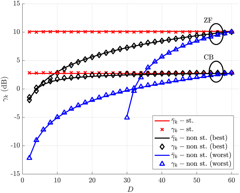
(b) Normalization 2: ${\rm tr}(\boldsymbol{\Theta})=D$.

Figure 2: The SINR vs the active number of antennas $D$ ($M=60$, $K=30$, and $\rho=$10\text{\,}\mathrm{dB}$$).

VI Conclusion

The VR of the channel impacts the performance of CB and ZF precoders significantly. For small VRs, the post processing SINR loss compared with the stationary channels can be as high as $15\text{\,}\mathrm{dB}$ for both CB and ZF. In the best-case, i.e., when the VRs of the users reduce inter-user interference, the post-processing SINR for both CB and ZF can be higher compared to a stationary channel. Finally, small VRs can make the channel rank deficient and render the ZF precoding infeasible.

Appendix A: Proof of Theorem 1

The SINR for ZF (8) can be re-written as

$$\gamma_{k}^{{{\mathrm{Z}}{\mathrm{F}}}}=p_{k}\frac{\rho}{\sum\limits_{i=1}^{K}p_{i}({\mathbf{H}}^{\ast}{\mathbf{H}})^{-1}_{i,i}},$$ (17)

where $({\mathbf{H}}^{\ast}{\mathbf{H}})^{-1}_{i,i}$ is the $i$th diagonal entry of the inverse matrix $({\mathbf{H}}^{\ast}{\mathbf{H}})^{-1}$. This entry can be re-written as

$$({\mathbf{H}}^{\ast}{\mathbf{H}})^{-1}_{i,i}=({\mathbf{h}}_{i}^{\ast}{\mathbf{h}}_{i}-{\mathbf{h}}_{i}^{\ast}\bar{\mathbf{H}}_{i}(\bar{\mathbf{H}}_{i}^{\ast}\bar{\mathbf{H}}_{i})^{-1}\bar{\mathbf{H}}_{i}^{\ast}{\mathbf{h}}_{i})^{-1},$$ (18)

where $\bar{\mathbf{H}}_{i}=[{\mathbf{h}}_{1},\leavevmode\nobreak\ \cdots,\leavevmode\nobreak\ {\mathbf{h}}_{i-1},\leavevmode\nobreak\ {\mathbf{h}}_{i+1},\leavevmode\nobreak\ \cdots,\leavevmode\nobreak\ {\mathbf{h}}_{K}]$. The first term on the RHS of (18) can be evaluated using (10) and [8, Lemma 4], i.e.,

$${\mathbf{z}}_{i}^{\ast}{\mathbf{R}}_{i}{\mathbf{z}}_{i}-\frac{1}{M}{\rm tr}({\mathbf{R}}_{i})\overset{\rm{a.s.}}{\underset{M\rightarrow\infty}{\longrightarrow}}0.$$ (19)

For the second term, we approximate $(\bar{\mathbf{H}}_{i}^{\ast}\bar{\mathbf{H}}_{i})^{-1}$ by retaining only its diagonal entries. For large $M$, approximating the off-diagonal terms to $0$ is reasonable as due to [8, Lemma 5]

$${\mathbf{z}}_{i}^{\ast}{\mathbf{R}}_{i}^{\frac{1}{2}}{\mathbf{R}}_{j}^{\frac{1}{2}}{\mathbf{z}}_{j}\overset{\rm{a.s.}}{\underset{M\rightarrow\infty}{\longrightarrow}}0.$$ (20)

We retain the diagonal entries in a matrix ${\mathbf{V}}_{i}$ defined as

$${\mathbf{V}}_{ij}=\begin{cases}(\bar{\mathbf{H}}_{i}^{\ast}\bar{\mathbf{H}}_{i})_{i,i}&\text{when }i=j,\\ 0&\text{otherwise}.\end{cases}$$ (21)

With the diagonal approximation, the second term on the RHS can be evaluated as

$${\mathbf{h}}_{i}^{\ast}\bar{\mathbf{H}}_{i}{\mathbf{V}}^{-1}\bar{\mathbf{H}}_{i}^{\ast}{\mathbf{h}}_{i}\overset{(a)}{=}{\rm tr}\big{(}\bar{\mathbf{H}}_{i}{\mathbf{V}}^{-1}\bar{\mathbf{H}}_{i}^{\ast}{\mathbf{R}}_{i}\big{)},\overset{(b)}{=}\sum\limits_{j=1,j\neq i}^{K}\frac{{\mathbf{h}}_{j}^{\ast}{\mathbf{R}}_{i}{\mathbf{h}}_{j}}{{\mathbf{h}}_{j}^{\ast}{\mathbf{h}}_{j}}\overset{(c)}{=}\sum\limits_{j=1,j\neq i}^{K}\frac{{\rm tr}({\mathbf{R}}_{i}{\mathbf{R}}_{j})}{{\rm tr}({\mathbf{R}}_{j})},$$ (22)

where $(a)$ is due to [8, Lemma 4], $(b)$ is by simple algebraic manipulation, and $(c)$ is due to the use of [8, Lemma 4] in both the numerator and denominator. We obtain (12) by using (19) and (22) in (17).

To guarantee the non-negativity of (12), it is sufficient to show that

$${\rm tr}({\mathbf{R}}_{i})-\sum\limits_{j=1,j\neq i}^{K}\frac{{\rm tr}({\mathbf{R}}_{i}{\mathbf{R}}_{j})}{{\rm tr}({\mathbf{R}}_{j})}\geq 0,\forall i.$$ (23)

If $\lambda_{\max}({\mathbf{R}}_{i})$ represents the largest eigenvalue of ${\mathbf{R}}_{i}$, then by using ${\rm tr}({\mathbf{R}}_{i})=M,\forall i$ and re-arranging terms in (23), we get

$$M^{2}\geq\sum\limits_{\begin{subarray}{c}j=1\\ j\neq i\end{subarray}}^{K}{\rm tr}({\mathbf{R}}_{i}{\mathbf{R}}_{j})\overset{(a)}{\geq}\sum\limits_{\begin{subarray}{c}j=1\\ j\neq i\end{subarray}}^{K}\lambda_{\max}({\mathbf{R}}_{i}){\rm tr}({\mathbf{R}}_{j})=M(K-1)\lambda_{\max}({\mathbf{R}}_{i}),$$ (24)

where $(a)$ is from the property ${\rm tr}({\mathbf{A}}{\mathbf{B}})\leq\lambda_{\max}({\mathbf{A}}){\rm tr}({\mathbf{B}})$ [10]. As $\lambda_{\max}({\mathbf{R}}_{i})$ is $\mathcal{O}(1)$ by A2, the above inequality is guaranteed to hold as $M/K\rightarrow\infty$.

Appendix B: Proof of Proposition 1

We can write $\bar{\mathbf{H}}_{i}^{\ast}\bar{\mathbf{H}}={\mathbf{V}}+{\mathbf{E}}$, where ${\mathbf{V}}$ is a diagonal matrix with terms of $O(M)$, and the matrix ${\mathbf{E}}$ has terms of $O(\sqrt{M})$. The first order Taylor series expansion of $(\bar{\mathbf{H}}_{i}^{\ast}\bar{\mathbf{H}})^{-1}$ gives

$$(\bar{\mathbf{H}}_{i}^{\ast}\bar{\mathbf{H}})^{-1}-{\mathbf{V}}^{-1}\approx-{\mathbf{V}}^{-1}{\mathbf{E}}{\mathbf{V}}^{-1}.$$ (25)

This result can be used in (13) to write the error as

$$\epsilon =|{\mathbf{h}}_{i}^{\ast}\bar{\mathbf{H}}_{i}({\mathbf{V}}^{-1}{\mathbf{E}}{\mathbf{V}}^{-1})\bar{\mathbf{H}}_{i}^{\ast}{\mathbf{h}}_{i}|.$$ (26)

The terms in the vector $\bar{\mathbf{H}}_{i}^{\ast}{\mathbf{h}}_{i}$ are $O(\sqrt{M})$. The terms in the matrix ${\mathbf{V}}^{-1}{\mathbf{E}}{\mathbf{V}}^{-1}$ are order $O(\frac{1}{\sqrt{M}^{3}})$. Thus the terms in the product vector ${\mathbf{V}}^{-1}{\mathbf{E}}{\mathbf{V}}^{-1}\bar{\mathbf{H}}_{i}^{\ast}{\mathbf{h}}_{i}$ are $O(\frac{\sqrt{K}}{M})$. Extending the same argument, the term ${\mathbf{h}}_{i}^{\ast}\bar{\mathbf{H}}_{i}({\mathbf{V}}^{-1}{\mathbf{E}}{\mathbf{V}}^{-1})\bar{\mathbf{H}}_{i}^{\ast}{\mathbf{h}}_{i}$ is $O(\frac{K}{\sqrt{M}})$. By using similar arguments, we can show that ${\mathbf{h}}_{i}^{\ast}\bar{\mathbf{H}}_{i}(\bar{\mathbf{H}}_{i}^{\ast}\bar{\mathbf{H}}_{i})^{-1}\bar{\mathbf{H}}_{i}^{\ast}{\mathbf{h}}_{i}$ is $O(K)$.

References

- [1] T. L. Marzetta, “Noncooperative cellular wireless with unlimited numbers of base station antennas,” IEEE Trans. Wireless Commun., vol. 9, no. 11, pp. 3590–3600, 2010.
- [2] À. O. Martínez, E. De Carvalho, and J. Ø. Nielsen, “Towards very large aperture massive MIMO: A measurement based study,” in Proc. IEEE Glob. Telecom. Conf. (GLOBECOM) Wksp, 2014, pp. 281–286.
- [3] S. Hu, F. Rusek, and O. Edfors, “Beyond Massive-MIMO: The Potential of Data-Transmission with Large Intelligent Surfaces,” arXiv preprint arXiv:1707.02887, 2017.
- [4] K. T. Truong and R. W. Heath Jr., “The viability of distributed antennas for massive MIMO systems,” in Proc. Asilomar Conf. Signals, Syst. Comput. (ASILOMAR), 2013, pp. 1318–1323.
- [5] Z. Zhou et al., “Spherical wave channel and analysis for large linear array in los conditions,” in Proc. IEEE Glob. Telecom. Conf. (GLOBECOM), 2015, pp. 1–6.
- [6] X. Li et al., “Capacity analysis for spatially non-wide sense stationary uplink Massive MIMO systems,” IEEE Trans. Wireless Commun., vol. 14, no. 12, pp. 7044–7056, 2015.
- [7] J. Hoydis, S. Ten Brink, and M. Debbah, “Massive MIMO in the UL/DL of cellular networks: How many antennas do we need?” IEEE J. Sel. Areas Commun., vol. 31, no. 2, pp. 160–171, 2013.
- [8] S. Wagner et al., “Large system analysis of linear precoding in correlated MISO broadcast channels under limited feedback,” IEEE Trans. Inf. Theory, vol. 58, no. 7, pp. 4509–4537, 2012.
- [9] E. Björnson et al., “Massive MIMO systems with non-ideal hardware: Energy efficiency, estimation, and capacity limits,” IEEE Trans. Inf. Theory, vol. 60, no. 11, pp. 7112–7139, 2014.
- [10] Y. Fang, K. A. Loparo, and X. Feng, “Inequalities for the trace of matrix product,” IEEE Trans. Autom. Control, vol. 39, no. 12, pp. 2489–2490, 1994.