Model of spin liquids with and without time-reversal symmetry

Abstract

We study a model in (2+1)-dimensional spacetime that is realized by an array of chains, each of which realizes relativistic Majorana fields in (1+1)-dimensional spacetime, coupled via current-current interactions. The model is shown to have a lattice realization in an array of two-leg quantum spin-$1/2$ ladders. We study the model both in the presence and absence of time-reversal symmetry, within a mean-field approximation. We find regimes in coupling space where Abelian and non-Abelian spin liquid phases are stable. In the case when the Hamiltonian is time-reversal symmetric, we find regimes where gapped Abelian and non-Abelian chiral phases appear as a result of spontaneous breaking of time-reversal symmetry. These gapped phases are separated by a discontinuous phase transition. More interestingly, we find a regime where a non-chiral gapless non-Abelian spin liquid is stable. The excitations in this regime are described by relativistic Majorana fields in (2+1)-dimensional spacetime, much as those appearing in the Kitaev honeycomb model, but here emerging in a model of coupled spin ladders that does not break $SU(2)$ spin-rotation symmetry.

I Motivation and summary of results

The Kalmeyer-Laughlin chiral spin liquid Kalmeyer and Laughlin (1987) was the first example of a connection between the physics of the fractional quantum Hall (FQH) effect and that of frustrated magnets that do not order via the spontaneous breaking of a symmetry. Such chiral spin liquids present exotic features, such as ground state degeneracy on the torus – a defining attribute of topological order Wen (1991). The Kitaev honeycomb model Kitaev (2006) presents another example of a chiral spin liquid when a gap is opened by the addition of a magnetic field. The Kitaev model displays, in a regime of parameters, non-Abelian topological order, where the quasiparticles obey non-Abelian braiding statistics, as in the Moore-Read FQH states.  Moore and Read (1991)

Recently, coupled-wire constructions pioneered by Kane and collaborators Mukhopadhyay et al. (2001); Kane et al. (2002); Teo and Kane (2014); Kane et al. (2017); Kane and Stern (2018) have provided a different approach to the construction of topological ordered states, in particular both Abelian and non-Abelian FQH states. These constructions allow one to utilize the powerful machinery of (1+1)-dimensional conformal field theory (CFT) to describe the individual quantum wires, which are then coupled to their neighbors to gap the bulk degrees of freedom of the resulting two-dimensional system. Gapless chiral modes, described by chiral CFTs Wen (1990), are rather naturally obtained in these coupled-wire constructions.

Most of the focus of coupled-wire constructions has been on electronic systems with a quantized (charge) Hall response. However, one may also use, instead of quantum wires, quantum spin chains or ladders, which can also be described by CFTs in their gapless limits. Gorohovsky et al. (2015); Huang et al. (2016); Lecheminant and Tsvelik (2017); Huang et al. (2017); Chen et al. (2017); Pereira and Bieri (2018) The result of these coupled-chain (or coupled-ladder) constructions are gapped chiral spin liquid in (2+1)-dimensional spacetime Kalmeyer and Laughlin (1987); Wen et al. (1989), much as the electronic wire constructions lead to gapped FQH states.

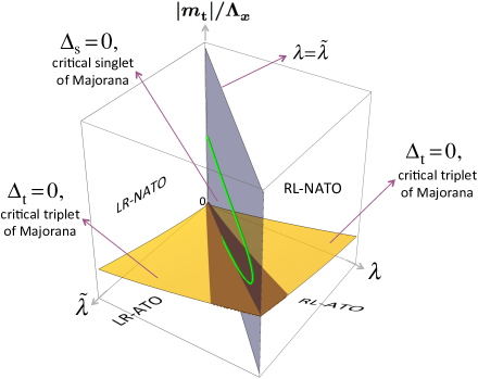
(a) (b)

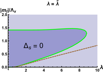
Figure 1: (Color online) (a) Mean-field phase diagram as a function of the three couplings $\lambda\geq 0$, $\widetilde{\lambda}\geq 0,$ and $|m^{\,}_{\mathrm{t}}|/\Lambda^{\,}_{x}$ for the theory defined in Eq. (4) under the assumptions (8) [$\Lambda^{\,}_{x}$ is a momentum cutoff that is introduced in Eq. (31b)]. The yellow (brown) surface represents those points in coupling space at which a continuous (discontinuous) mean-field transition separates two distinct gapped phases of matter, the mean-field snapshots of an Abelian topological order (ATO) phase and a non-Abelian topological order (NATO) phase, respectively. The quadrant $\lambda=\widetilde{\lambda}$ is colored in grey and is explained in the panel (b). (b) For $|m^{\,}_{\mathrm{t}}/\Lambda^{\,}_{x}|\geq 0$ and $\lambda=\widetilde{\lambda}\geq 0$, the region bounded by the vertical axis and the continuous line (colored in green) supports a time-reversal symmetric mean-field solution ($\Phi^{\,}_{-}=0$) as the minima of the mean-field potential, with the vanishing singlet gap $\Delta^{\,}_{\mathrm{s}}=0$ and the non-vanishing triplet gap $\Delta^{\,}_{\mathrm{t}}=2|m^{\,}_{\mathrm{t}}|\neq 0$ defined by Eq. (38). Outside of this region, time-reversal symmetry is spontaneously broken at the mean-field level ($\Phi^{\,}_{-}\neq 0$) with non-vanishing singlet ($\Delta^{\,}_{\mathrm{s}}\neq 0$) and triplet ($\Delta^{\,}_{\mathrm{t}}\neq 0$) gaps defined by Eq. (38). The dashed line (colored in brown) is a line of discontinuous phase transitions by which $|\Phi^{\,}_{-}|<|m^{\,}_{\mathrm{t}}|$ above the dashed line while $|\Phi^{\,}_{-}|>|m^{\,}_{\mathrm{t}}|$ below the dashed line. It separates the mean-field snapshot of an ATO from a NATO phase.

Within this coupled-ladder approach, we presented a model in Ref. Chen et al., 2017 that we argued displayed both Abelian and non-Abelian chiral spin liquid phases. In that model, each two-legged ladder (central charge $c=2$) can be described using four flavors of Majorana fields ($c=1/2$ each). These four fields in each “wire” can be split into triplet and singlet representation of $SU(2)$. The Majorana fields are local within each “wire”, as quadratic terms (such as back-scattering) are only allowed inside the one-dimensional channels; we denote such mass terms for the triplet and singlet Majorana fields by $m^{\,}_{\mathrm{t}}$ and $m^{\,}_{\mathrm{s}}$. In contrast, local inter-ladder interactions are necessarily quartic in the Majorana fields, and characterized by couplings constants $\lambda,\widetilde{\lambda}$, which are introduced in Sec. II. In Ref. Chen et al., 2017 we studied the case $\lambda\neq 0,\widetilde{\lambda}=0$, which maximally breaks time-reversal symmetry (TRS). This limit was analyzed using mean-field theory and a random phase approximation that started from an exactly solvable limit. Within these approximations, we obtained the phase diagram of the coupled-ladder system, with its gapped Abelian and non-Abelian chiral phases.

Summary of results: the phase diagram

In the present work, we consider generic inter-ladder interactions, $\lambda,\widetilde{\lambda}\neq 0$, that encompass the case $\lambda=\widetilde{\lambda}$ where TRS is not explicitly broken, and we search for non-chiral spin liquids within the coupled ladder system. We find a rather rich phase diagram within a mean-field approximation, which we depict in Fig. 1. The phase diagram includes the gapped chiral Abelian and non-Abelian phases when TRS is either explicitly or spontaneously broken. In the case where TRS is spontaneously broken, we find that the Abelian and non-Abelian phases are separated by a discontinuous transition. More interestingly, we identify a regime where TRS remains unbroken, leading to a gapless non-chiral spin liquid. At the gapless region, the Majorana fields acquire dispersion in the direction perpendicular to the ladders, yielding a pair of 2D Majorana cones. We thus find an example of a spin system with full $SU(2)$ spin-rotation invariance that supports a non-chiral spin liquid phase with gapless Majoranas as in the phase B of Kitaev honeycomb model. However, $SU(2)$ spin-rotation symmetry is absent in the Kitaev honeycomb model.

The paper is organized as follows. We present the model of coupled Majorana fields and analyze several of its symmetries in Sec. II. We then study the model within a mean-field treatment in Sec. III. In Sec. IV, we discuss possible implications of the mean-field phase diagram for a model of coupled spin-ladder, whose couplings are contained within the coupled Majorana field theory. We summarize our results in Sec. V.

II Model of coupled Majorana field theories

II.1 Definition

Our quantum-field theory is built from four species (labeled by $\mu=0,\cdots,3$) of Majorana fields whose support is $(1+1)$-dimensional spacetime. We will call this building-block a “ladder”. This terminology is justified by the fact that we find in Sec. IV a spin-1/2 ladder that regularizes this quantum field theory. We then consider $n$ independent copies of the Majorana quantum-field theory in $(1+1)$-dimensional spacetime with the kinetic Hamiltonian density

$$\widehat{\mathcal{H}}^{\,}_{0}\,\raisebox{0.85pt}{.}\raisebox{2.85pt}{.}\!\!=\,\sum^{n}_{\mathtt{m}=1}\sum^{3}_{\mu=0}\frac{\mathrm{i}}{2}v^{\,}_{\mu}\left(\widehat{\chi}^{\mu}_{\mathrm{L},\mathtt{m}}\partial^{\,}_{x}\widehat{\chi}^{\mu}_{\mathrm{L},\mathtt{m}}-\widehat{\chi}^{\mu}_{\mathrm{R},\mathtt{m}}\partial^{\,}_{x}\widehat{\chi}^{\mu}_{\mathrm{R},\mathtt{m}}\right),$$ (1)

where the velocities $v^{\,}_{\mu}$ are real valued and $\mathrm{L},\mathrm{R}$ denotes the left- and right-movers, respectively. The Majorana fields, $(\widehat{\chi}^{\mu}_{\mathrm{M},\mathtt{m}})^{*}=\widehat{\chi}^{\mu}_{\mathrm{M},\mathtt{m}}$, obey the equal-time anti-commutators $\left\{\widehat{\chi}^{\mu}_{\mathrm{M},\mathtt{m}}(x),\widehat{\chi}^{\mu^{\prime}}_{\mathrm{M}^{\prime},\mathtt{m}^{\prime}}(x^{\prime})\right\}=\delta^{\,}_{\mathrm{M}\mathrm{M}^{\prime}}\,\delta^{\,}_{\mathtt{m}\mathtt{m}^{\prime}}\,\delta^{\,}_{\mu\mu^{\prime}}\,\delta(x-x^{\prime}),$ with $\mu,\mu^{\prime}=0,\cdots 3,$ $\mathrm{M},\mathrm{M}^{\prime}=\mathrm{L},\mathrm{R}$, $\mathtt{m},\mathtt{m}^{\prime}=1,\cdots,n$, and $0\leq x\leq L^{\,}_{x}.$

Besides the kinetic term (1), we assume that there is a back-scattering term with real valued couplings $m^{\,}_{\mu}$ ($\mu=0,\cdots,3$) inside each ladder

$$\widehat{\mathcal{H}}^{\,}_{\mathrm{intra}-\mathrm{ladder}}\,\raisebox{0.85pt}{.}\raisebox{2.85pt}{.}\!\!=\,\sum^{n}_{\mathtt{m}=1}\sum^{3}_{\mu=0}\mathrm{i}\,m^{\,}_{\mu}\,\widehat{\chi}^{\mu}_{\mathrm{L},\mathtt{m}}\widehat{\chi}^{\mu}_{\mathrm{R},\mathtt{m}}.$$ (2)

We then couple consecutive ladders by considering inter-ladder quartic interactions with real valued coupling constants $\lambda$ and $\widetilde{\lambda}$

$$\widehat{\mathcal{H}}^{\,}_{\mathrm{inter}-\mathrm{ladder}}\,\raisebox{0.85pt}{.}\raisebox{2.85pt}{.}\!\!=\,\sum^{n-1}_{\mathtt{m}=1}\left(\widehat{\mathcal{H}}^{\,}_{\lambda,\mathtt{m}}+\widehat{\mathcal{H}}^{\,}_{\widetilde{\lambda},\mathtt{m}}\right),$$ (3a)

$$\widehat{\mathcal{H}}^{\,}_{\lambda,\mathtt{m}}\,\raisebox{0.85pt}{.}\raisebox{2.85pt}{.}\!\!=\,\frac{\lambda\vphantom{\widetilde{\lambda}}}{4}\left(\sum^{3}_{\mu=0}\widehat{\chi}^{\mu}_{\mathrm{L},\mathtt{m}}\,\widehat{\chi}^{\mu}_{\mathrm{R},\mathtt{m}+1}\,\right)^{2},$$ (3b)

$$\widehat{\mathcal{H}}^{\,}_{\widetilde{\lambda},\mathtt{m}}\,\raisebox{0.85pt}{.}\raisebox{2.85pt}{.}\!\!=\,\frac{\widetilde{\lambda}}{4}\left(\sum^{3}_{\mu=0}\widehat{\chi}^{\mu}_{\mathrm{R},\mathtt{m}}\,\widehat{\chi}^{\mu}_{\mathrm{L},\mathtt{m}+1}\,\right)^{2}.$$ (3c)

Each $\widehat{\mathcal{H}}^{\,}_{\lambda,\mathtt{m}}$ and $\widehat{\mathcal{H}}^{\,}_{\widetilde{\lambda},\mathtt{m}}$ term alone is the $O(4)$ Gross-Neveu-like quartic interaction.

The final Hamiltonian density is

$$\widehat{\mathcal{H}}\,\raisebox{0.85pt}{.}\raisebox{2.85pt}{.}\!\!=\,\widehat{\mathcal{H}}^{\,}_{0}+\widehat{\mathcal{H}}^{\,}_{\mathrm{intra}-\mathrm{ladder}}+\widehat{\mathcal{H}}^{\,}_{\mathrm{inter}-\mathrm{ladder}},$$ (4)

with $\widehat{\mathcal{H}}^{\,}_{0}$, $\widehat{\mathcal{H}}^{\,}_{\mathrm{intra}-\mathrm{ladder}}$ and $\widehat{\mathcal{H}}^{\,}_{\mathrm{inter}-\mathrm{ladder}}$ defined in Eq. (1), (2) and (3), respectively.

The limit $\widetilde{\lambda}=0$ in the Hamiltonian density (4) was considered in Ref. Chen et al., 2017. This regime corresponds (with the singlet mass $m^{\,}_{\mathrm{s}}=0$) to the planar region $(\lambda\geq 0,\widetilde{\lambda}=0,m^{\,}_{\mathrm{t}}>0,m^{\,}_{\mathrm{s}}=0)$ in Fig. 1, where ATO and NATO are the abbreviations for “Abelian topological order” and “non-Abelian topological order”, respectively. A telltale to distinguish these phases is the central charge $c$ of edge states: For Abelian phases, $c$ is necessarily integer; instead, if $c$ is fractional, the phase is necessarily non-Abelian. (Notice that it is possible to have integer $c$ for non-Abelian phases, for instance direct sums of models with fractional $c$’s that add up to an integer.) In our model, the signatures of these phases at the mean-field level are the following. The edge states of a mean-field snapshot of the ATO phase are quadruplet of right-moving (left-moving) Majorana fermions $\widehat{\chi}^{\mu}_{\mathrm{R},1}$ ($\widehat{\chi}^{\mu}_{\mathrm{L},n}$) on the first (last) edge for $\mu=0,1,2,3$, yielding $c=4\times 1/2=2\in\mathbb{Z}$. The edge states of a mean-field snapshot of the NATO phase consist of the singlet Majorana modes $\widehat{\chi}^{0}_{\mathrm{R},1}$ and $\widehat{\chi}^{0}_{\mathrm{L},n}$, with $c=1\times 1/2=1/2\notin\mathbb{Z}$.

The goal of this work is to study the generic case where both $\lambda$ and $\widetilde{\lambda}$ are non-zero. The phase diagram in Fig. 1 is mirror symmetric about the plane $\lambda=\widetilde{\lambda}$, and we shall be particularly interested in the limit $\lambda=\widetilde{\lambda}$ at which the Hamiltonian density (4) is invariant under TRS.

II.2 Symmetries

Reversal of time is implemented by the $\mathtt{m}$-resolved antiunitary $\mathbb{Z}^{\,}_{2}$ transformation by which

$$\begin{split}&\widehat{\chi}^{\mu}_{\mathrm{L},\mathtt{m}}(x)\;\mapsto\;\widehat{\chi}^{\mu}_{\mathrm{R},\mathtt{m}}(x),\\ &\widehat{\chi}^{\mu}_{\mathrm{R},\mathtt{m}}(x)\;\mapsto\;\widehat{\chi}^{\mu}_{\mathrm{L},\mathtt{m}}(x),\\ &\mathrm{i}\;\mapsto\;-\mathrm{i},\end{split}$$ (5)

for any $\mu=0,\cdots,3$, $\mathtt{m}=1,\cdots,n$, and $0\leq x\leq L^{\,}_{x}$.

The Hamiltonian density (4) has more symmetries. First, for arbitrary values of the masses and the couplings, the Hamiltonian density (4) is invariant under

$$\widehat{\chi}^{\mu}_{\mathrm{M},\mathtt{m}}(x)\;\mapsto\;\sigma^{\mu}\,\widehat{\chi}^{\mu}_{\mathrm{M},\mathtt{m}}(x),\qquad\sigma^{\mu}=\pm 1,$$ (6)

for any $\mu=0,\cdots,3$, $\mathrm{M}=\mathrm{L},\mathrm{R}$, $\mathtt{m}=1,\cdots,n$, and $0\leq x\leq L^{\,}_{x}$. Second, it is also invariant under the $\mathtt{m}$-resolved (local) $\mathbb{Z}^{\,}_{2}$ transformation by which

$$\widehat{\chi}^{\mu}_{\mathrm{M},\mathtt{m}}(x)\;\mapsto\;\sigma^{\,}_{\mathtt{m}}\,\widehat{\chi}^{\mu}_{\mathrm{M},\mathtt{m}}(x),\qquad\sigma^{\,}_{\mathtt{m}}=\pm 1,$$ (7)

for any $\mu=0,\cdots,3$, $\mathrm{M}=\mathrm{L},\mathrm{R}$, $\mathtt{m}=1,\cdots,n$, and $0\leq x\leq L^{\,}_{x}$.

Whenever the underlying lattice regularization of the Hamiltonian density (4) is endowed with a global $SU(2)$ symmetry, we will impose the conditions

$$\begin{split}&v^{\,}_{0}\equiv v^{\,}_{\mathrm{s}}\equiv v,\qquad m^{\,}_{0}\equiv m^{\,}_{\mathrm{s}}=0,\\ &v^{\,}_{a}\equiv v^{\,}_{\mathrm{t}}\equiv v,\qquad m^{\,}_{a}\equiv m^{\,}_{\mathrm{t}},\qquad a=1,2,3,\end{split}$$ (8)

where $\mathrm{s}$ and $\mathrm{t}$ stands for “singlet” and “triplet”, respectively.

III Mean-field approach

III.1 Two auxiliary scalar fields

We will treat the inter-ladder quartic interactions (3) by performing a Hubbard-Stratonovich transformation. To this end, we employ the Euclidean path-integral formalism and introduce two real-valued auxiliary scalar fields, $\phi^{\,}_{\mathtt{m},\mathtt{m}+1}$ and $\tilde{\phi}^{\,}_{\mathtt{m},\mathtt{m}+1}$ for $\mathtt{m}=1,\cdots,n-1.$ The model (4) can then be written as

$$Z\,\raisebox{0.85pt}{.}\raisebox{2.85pt}{.}\!\!=\,\int\mathcal{D}[\phi,\tilde{\phi}]\int\mathcal{D}[\chi^{0},\chi^{1},\chi^{2},\chi^{3}]\,e^{-S},$$ (9a)

$$S\,\raisebox{0.85pt}{.}\raisebox{2.85pt}{.}\!\!=\,\int\limits_{0}^{\beta}\mathrm{d}\tau\,\int\limits_{0}^{L^{\,}_{x}}\mathrm{d}x\,\sum_{\mathtt{m}=1}^{L^{\,}_{y}/\mathfrak{a}^{\,}_{y}}\left(\mathcal{L}^{\,}_{\mathrm{f},\mathtt{m}}+\mathcal{L}^{\,}_{\mathrm{b},\mathtt{m}}+\mathcal{L}^{\,}_{\mathrm{fb},\mathtt{m}}\right),$$ (9b)

$$\mathcal{L}^{\,}_{\mathrm{f},\mathtt{m}}\,\raisebox{0.85pt}{.}\raisebox{2.85pt}{.}\!\!=\,\frac{1}{2}\sum^{3}_{\mu=0}\Big{[}\chi^{\mu}_{\mathrm{L},\mathtt{m}}\left(\partial^{\,}_{\tau}+\mathrm{i}v^{\,}_{\mu}\partial^{\,}_{x}\right)\chi^{\mu}_{\mathrm{L},\mathtt{m}}$$

$$\hskip 60.00009pt+\chi^{\mu}_{\mathrm{R},\mathtt{m}}\left(\partial^{\,}_{\tau}-\mathrm{i}v^{\,}_{\mu}\partial^{\,}_{x}\right)\chi^{\mu}_{\mathrm{R},\mathtt{m}}\Big{]}$$

$$\hskip 30.00005pt+\sum_{\mu=0}^{3}\mathrm{i}\,m^{\,}_{\mu}\chi^{\mu}_{\mathrm{L},\mathtt{m}}\,\chi^{\mu}_{\mathrm{R},\mathtt{m}},$$ (9c)

$$\mathcal{L}^{\,}_{\mathrm{b},\mathtt{m}}\,\raisebox{0.85pt}{.}\raisebox{2.85pt}{.}\!\!=\,\frac{1}{4\,\lambda}(\phi^{\,}_{\mathtt{m},\mathtt{m}+1})^{2}+\frac{1}{4\,\widetilde{\lambda}}(\tilde{\phi}^{\,}_{\mathtt{m},\mathtt{m}+1})^{2},$$ (9d)

$$\mathcal{L}^{\,}_{\mathrm{fb},\mathtt{m}}\,\raisebox{0.85pt}{.}\raisebox{2.85pt}{.}\!\!=\,\sum_{\mu=0}^{3}\frac{1}{2}\left(-\mathrm{i}\chi^{\mu}_{\mathrm{L},\mathtt{m}}\,\chi^{\mu}_{\mathrm{R},\mathtt{m}+1}\right)\phi^{\,}_{\mathtt{m},\mathtt{m}+1}$$

$$\hphantom{\mathcal{L}^{\,}_{\chi,\phi,\mathtt{m}}\,\raisebox{0.85pt}{.}\raisebox{2.85pt}{.}\!\!=\,}+\sum_{\mu=0}^{3}\frac{1}{2}\left(-\mathrm{i}\chi^{\mu}_{\mathrm{R},\mathtt{m}}\,\chi^{\mu}_{\mathrm{L},\mathtt{m}+1}\right)\tilde{\phi}^{\,}_{\mathtt{m},\mathtt{m}+1}.$$ (9e)

Here, $\beta$ is the inverse temperature and $\mathfrak{a}^{\,}_{y}$ is the spacing between two consecutive ladders.

III.2 Symmetries

The action (9b) with $\lambda=\widetilde{\lambda}$ is invariant under the $\mathtt{m}$-resolved antiunitary time-reversal transformation [c.f. Eq. (5)]

$$\begin{split}\chi^{\mu}_{\mathrm{M},\mathtt{m}}(\tau,x)&\;\mapsto\;\chi^{\mu}_{\mathrm{M}^{\prime},\mathtt{m}}(\tau,x),\qquad\mathrm{M}\neq\mathrm{M}^{\prime},\\ \phi^{\,}_{\mathtt{m},\mathtt{m}+1}(\tau,x)&\;\mapsto\;-\,\tilde{\phi}^{\,}_{\mathtt{m},\mathtt{m}+1}(\tau,x),\\ \tilde{\phi}^{\,}_{\mathtt{m},\mathtt{m}+1}(\tau,x)&\;\mapsto\;-\,\phi^{\,}_{\mathtt{m},\mathtt{m}+1}(\tau,x),\end{split}$$ (10)

for any $\mu=0,\cdots,3$, $\mathrm{M}=\mathrm{L},\mathrm{R}$, $\mathtt{m}=1,\cdots,n$, $0\leq\tau\leq\beta$, and $0\leq x\leq L^{\,}_{x}$.

The action (9b) has the following additional symmetries. First, the $\mu$-resolved Majorana parity is conserved owing to the symmetry of the action $S$ (9b) under the $\mathbb{Z}^{\,}_{2}$ transformation [c.f. Eq. (6)]

$$\chi^{\mu}_{\mathrm{M},\mathtt{m}}(\tau,x)\;\mapsto\;\sigma^{\mu}\,\chi^{\mu}_{\mathrm{M},\mathtt{m}}(\tau,x),\qquad\sigma^{\mu}=\pm 1,$$ (11)

for any $\mu=0,\cdots,3$, $\mathrm{M}=\mathrm{L},\mathrm{R}$, $\mathtt{m}=1,\cdots,n$, $0\leq\tau\leq\beta$, and $0\leq x\leq L^{\,}_{x}$.

Second, the action (9b) is invariant under the $\mathtt{m}$-resolved $\mathbb{Z}^{\,}_{2}$ transformation [c.f. Eq. (7)]

$$\begin{split}\chi^{\mu}_{\mathrm{M},\mathtt{m}}(\tau,x)&\;\mapsto\;\sigma^{\,}_{\mathtt{m}}\,\chi^{\mu}_{\mathrm{M},\mathtt{m}}(\tau,x),\qquad\sigma^{\,}_{\mathtt{m}}=\pm 1,\\ \phi^{\,}_{\mathtt{m},\mathtt{m}+1}(\tau,x)&\;\mapsto\;\sigma^{\,}_{\mathtt{m}}\,\sigma^{\,}_{\mathtt{m}+1}\,\phi^{\,}_{\mathtt{m},\mathtt{m}+1}(\tau,x),\\ \tilde{\phi}^{\,}_{\mathtt{m},\mathtt{m}+1}(\tau,x)&\;\mapsto\;\sigma^{\,}_{\mathtt{m}}\,\sigma^{\,}_{\mathtt{m}+1}\,\tilde{\phi}^{\,}_{\mathtt{m},\mathtt{m}+1}(\tau,x),\end{split}$$ (12)

for any $\mu=0,\cdots,3$, $\mathrm{M}=\mathrm{L},\mathrm{R}$, $\mathtt{m}=1,\cdots,n$, $0\leq\tau\leq\beta$, and $0\leq x\leq L^{\,}_{x}$.

III.3 Mean-field single-particle Hamiltonian

We do the mean-field approximation by which the Hubbard-Stratonovich fields $\phi$ and $\tilde{\phi}$ are assumed independent of the spacetime coordinates $(\tau,x)$ and the ladder index $\mathtt{m}$,

$$\phi^{\,}_{\mathtt{m},\mathtt{m}+1}(\tau,x)\equiv\phi,\qquad\tilde{\phi}^{\,}_{\mathtt{m},\mathtt{m}+1}(\tau,x)\equiv\tilde{\phi}.$$ (13)

In what follows, we will ignore sign fluctuations of these Hubbard-Stratonovich fields $\phi$ and $\tilde{\phi}$, since as was demonstrated in Ref. Assaad and Grover, 2016, where fermions coupled to a $\mathbb{Z}^{\,}_{2}$ gauge field on a square lattice were studied, such fluctuations are irrelevant. If so, the action from (9d) simplifies to

$$S^{\,}_{\mathrm{b}}\,\raisebox{0.85pt}{.}\raisebox{2.85pt}{.}\!\!=\, \int\limits_{0}^{\beta}\mathrm{d}\tau\int\limits_{0}^{L^{\,}_{x}}\mathrm{d}x\,\sum_{\mathtt{m}=1}^{L^{\,}_{y}/\mathfrak{a}^{\,}_{y}}\,\mathcal{L}^{\,}_{\mathrm{b},\mathtt{m}}$$

$$= \,\beta\,L^{\,}_{x}\,\frac{L^{\,}_{y}}{\mathfrak{a}^{\,}_{y}}\left(\frac{1}{4\lambda}\phi^{2}+\frac{1}{4\widetilde{\lambda}}\tilde{\phi}^{2}\right).$$ (14)

We proceed by imposing periodic boundary condition along the $y$-direction, $\chi^{\mu}_{\mathrm{M},n+1}\equiv\chi^{\mu}_{\mathrm{M},1}$ for $\mathrm{M}=\mathrm{L},\mathrm{R}$, and by performing the Fourier transformation

$$S^{\,}_{\mathrm{f}}+S^{\,}_{\mathrm{fb}}\,\raisebox{0.85pt}{.}\raisebox{2.85pt}{.}\!\!=\,\int\limits_{0}^{\beta}\mathrm{d}\tau\int\limits_{0}^{L^{\,}_{x}}\mathrm{d}x\,\sum_{\mathtt{m}=1}^{L^{\,}_{y}/\mathfrak{a}^{\,}_{y}}\,\left(\mathcal{L}^{\,}_{\mathrm{f},\mathtt{m}}+\mathcal{L}^{\,}_{\mathrm{fb},\mathtt{m}}\right)=\sum^{\,}_{\omega,\bm{k}}\,\sum^{3}_{\mu=0}\frac{1}{2}\left(\chi^{\mu}_{-\omega,-\bm{k}}\right)^{\mathrm{T}}\left(\mathrm{i}\omega\sigma^{\,}_{0}+\widehat{H}^{\mathrm{MF}}_{\mu,\bm{k}}\right)\chi^{\mu}_{\omega,\bm{k}},$$ (15a)

where $$\chi^{\mu}_{\omega,\bm{k}}:=\left(\chi^{\mu}_{\mathrm{R},\omega,\bm{k}},\chi^{\mu}_{\mathrm{L},\omega,\bm{k}}\right)^{\mathsf{T}} \mu=0,\cdots,3$$ for each flavor , the mean-field Majorana Hamiltonian is

$$\widehat{H}^{\mathrm{MF}}_{\mu,\bm{k}}\,\raisebox{0.85pt}{.}\raisebox{2.85pt}{.}\!\!=\,-v^{\,}_{\mu}k^{\,}_{x}\,\sigma^{\,}_{3}-\Phi^{\,}_{+}\sin\left(k^{\,}_{y}\mathfrak{a}^{\,}_{y}\right)\sigma^{\,}_{1}+\left[m^{\,}_{\mu}-\Phi^{\,}_{-}\cos\left(k^{\,}_{y}\mathfrak{a}^{\,}_{y}\right)\right]\,\sigma^{\,}_{2},$$ (15b)

and we have introduced the linear combinations

$$\Phi^{\,}_{\pm}\,\raisebox{0.85pt}{.}\raisebox{2.85pt}{.}\!\!=\,\frac{1}{2}\left(\phi\pm\tilde{\phi}\right),$$ (15c)

for the auxiliary scalar fields. Here, $\sigma^{\,}_{1}$, $\sigma^{\,}_{2}$, and $\sigma^{\,}_{3}$ are Pauli matrices, while $\sigma^{\,}_{0}$ is the $2\times 2$ identity matrix.

We can diagonalize the $2\times 2$ single-particle Hamiltonian (15b) for each flavor $\mu=0,\cdots,3$. There follows eight branches of mean-field excitations with the dispersions (we have set $\mathfrak{a}^{\,}_{y}=1$)

$$\varepsilon^{\,}_{\mu,\pm}(k^{\,}_{x},k^{\,}_{y})\,\raisebox{0.85pt}{.}\raisebox{2.85pt}{.}\!\!=\,\pm\varepsilon^{\,}_{\mu}(k^{\,}_{x},k^{\,}_{y}),$$ (16a)

$$\varepsilon^{\,}_{\mu}(k^{\,}_{x},k^{\,}_{y})\,\raisebox{0.85pt}{.}\raisebox{2.85pt}{.}\!\!=\,\sqrt{v^{2}_{\mu}k^{2}_{x}+\left(m^{\,}_{\mu}-\Phi^{\,}_{-}\cos k^{\,}_{y}\right)^{2}+\Phi^{2}_{+}\sin^{2}k^{\,}_{y}}.$$ (16b)

We see that the eight branches fall into four pairs of particle-hole symmetric bands. For arbitrary value of $k^{\,}_{x}$ and $k^{\,}_{y},$ the mean-field Majorana direct gap is defined by

$$\Delta^{\,}_{\mu}(k^{\,}_{x},k^{\,}_{y})\,\raisebox{0.85pt}{.}\raisebox{2.85pt}{.}\!\!=\, \,\varepsilon^{\,}_{+,\mu}(k^{\,}_{x},k^{\,}_{y})-\varepsilon^{\,}_{-,\mu}(k^{\,}_{x},k^{\,}_{y})$$

$$= \,2\,\varepsilon^{\,}_{\mu}(k^{\,}_{x},k^{\,}_{y}).$$ (17)

In the vicinity of $(k^{\,}_{x}=0,k^{\,}_{y}=0)$ and $(k^{\,}_{x}=0,k^{\,}_{y}=\pi)$, the mean-field Majorana direct gaps are,

$$\Delta^{\,}_{\mu,}(0,0)=2\left|m^{\,}_{\mu}-\Phi^{\,}_{-}\right|=2\left|m^{\,}_{\mu}-\frac{\phi}{2}+\frac{\tilde{\phi}}{2}\right|,$$ (18a)

and

$$\Delta^{\,}_{\mu}(0,\pi)=2\left|m^{\,}_{\mu}+\Phi^{\,}_{-}\right|=2\left|m^{\,}_{\mu}+\frac{\phi}{2}-\frac{\tilde{\phi}}{2}\right|,$$ (18b)

respectively. The miminum of the two gap functions (18) is

$$\Delta^{\,}_{\mu}\,\raisebox{0.85pt}{.}\raisebox{2.85pt}{.}\!\!=\, \,2\left||m^{\,}_{\mu}|-\left|\Phi^{\,}_{-}\right|\right|=2\left||m^{\,}_{\mu}|-\frac{1}{2}\left|\phi-\tilde{\phi}\right|\right|.$$ (19)

III.4 Linearized spectrum

The physics captured by the mean-field Majorana single-particle Hamiltonian (15b) becomes more transparent upon linearizing the latter around the gap closing points $(k^{\,}_{x},k^{\,}_{y})=(0,0)$ and $(k^{\,}_{x},k^{\,}_{y})=(0,\pi/\mathfrak{a}^{\,}_{y})$, respectively. One finds

$$\widehat{H}^{\mathrm{MF}}_{\mu,k^{\,}_{x}=0+p^{\,}_{x},k^{\,}_{y}=0+p^{\,}_{y}}\approx-v^{\,}_{\mu}\,p^{\,}_{x}\,\sigma^{\,}_{3}-\mathfrak{a}^{\,}_{y}\,\Phi^{\,}_{+}\,p^{\,}_{y}\,\sigma^{\,}_{1}+\left(m^{\,}_{\mu}-\Phi^{\,}_{-}\right)\,\sigma^{\,}_{2},$$ (20a)

$$\widehat{H}^{\mathrm{MF}}_{\mu,k^{\,}_{x}=0+p^{\,}_{x},k^{\,}_{y}=(\pi/\mathfrak{a}^{\,}_{y})+p^{\,}_{y}}\approx-v^{\,}_{\mu}\,p^{\,}_{x}\,\sigma^{\,}_{3}+\mathfrak{a}^{\,}_{y}\,\Phi^{\,}_{+}\,p^{\,}_{y}\,\sigma^{\,}_{1}+\left(m^{\,}_{\mu}+\Phi^{\,}_{-}\right)\,\sigma^{\,}_{2}.$$ (20b)

Accordingly, $\mathfrak{a}^{\,}_{y}\Phi^{\,}_{+}$ plays the role of the Fermi velocity in the $y$-direction. Furthermore, we find that the single-particle Majorana gap is 2$\left|m^{\,}_{\mu}\mp\Phi^{\,}_{-}\right|$, in agreement with Eqs. (18a) and (18b). We now combine these linearized mean-field Majorana single-particle Hamiltonian into the $4\times 4$ matrix

$$\widehat{H}^{\mathrm{MF},\mathrm{lin}}_{\mu,\bm{p}}\,\raisebox{0.85pt}{.}\raisebox{2.85pt}{.}\!\!=\, \,\begin{pmatrix}\widehat{H}^{\mathrm{MF}}_{\mu,k^{\,}_{x}=0+p^{\,}_{x},k^{\,}_{y}=0+p^{\,}_{y}}&0^{\,}_{2\times 2}\\ 0^{\,}_{2\times 2}&\widehat{H}^{\mathrm{MF}}_{\mu,k^{\,}_{x}=0+p^{\,}_{x},k^{\,}_{y}=(\pi/\mathfrak{a}^{\,}_{y})+p^{\,}_{y}}\end{pmatrix}$$

$$= \,-v^{\,}_{x,\mu}\,p^{\,}_{x}\,\sigma^{\,}_{3}\otimes\tau^{\,}_{0}-v^{\,}_{y}\,p^{\,}_{y}\,\sigma^{\,}_{1}\otimes\tau^{\,}_{3}+m^{\,}_{\mu}\,\sigma^{\,}_{2}\otimes\tau^{\,}_{0}-\Phi^{\,}_{-}\,\sigma^{\,}_{2}\otimes\tau^{\,}_{3},$$ (21a)

where we have defined

$$v^{\,}_{x,\mu}\,\raisebox{0.85pt}{.}\raisebox{2.85pt}{.}\!\!=\,v^{\,}_{\mu},\qquad v^{\,}_{y}\,\raisebox{0.85pt}{.}\raisebox{2.85pt}{.}\!\!=\,\mathfrak{a}^{\,}_{y}\Phi^{\,}_{+}.$$ (21b)

This is an anisotropic single-particle Dirac Hamiltonian. The anisotropy enters through the two distinct Fermi velocities (21b), with the velocity along the $y$ direction emerging from the non-vanishing value $\Phi^{\,}_{+}$ for the bonding linear combination of the Hubbard-Stratonovich fields. There are two competing masses, $m^{\,}_{\mu}$ and the anti-bonding linear combination $\Phi^{\,}_{-}$ of the Hubbard-Stratonovich fields that measures the amount by which the mean-field breaks time-reversal symmetry. These masses compete because they multiply two $4\times 4$ matrices that commute,

$$\left[\sigma^{\,}_{2}\otimes\tau^{\,}_{0},\sigma^{\,}_{2}\otimes\tau^{\,}_{3}\right]=0.$$ (22)

The mass term $m^{\,}_{\mu}\,\sigma^{\,}_{2}\otimes\tau^{\,}_{0}$ breaks a unitary $\mathbb{Z}^{\,}_{2}$ symmetry represented by conjugation with

$$\hat{\mathcal{I}}=\sigma^{\,}_{3}\otimes\tau^{\,}_{1}.$$ (23)

The mass term $\Phi^{\,}_{-}\,\sigma^{\,}_{2}\otimes\tau^{\,}_{3}$ breaks time-reversal symmetry that is represented by conjugation with

$$\hat{\mathcal{T}}=\sigma^{\,}_{1}\otimes\tau^{\,}_{1}\,\mathsf{K},$$ (24)

where $\mathsf{K}$ denotes the complex conjugation.

The competition between the mass terms $m^{\,}_{\mu}\,\sigma^{\,}_{2}\otimes\tau^{\,}_{0}$ and $\Phi^{\,}_{-}\,\sigma^{\,}_{2}\otimes\tau^{\,}_{3}$ implies a gap closing (i.e., continuous) transition when

$$|m^{\,}_{\mu}|=|\Phi^{\,}_{-}|$$ (25)

that separates two single-particle insulating phases. As shown by Haldane Haldane (1988), the Chern numbers for the pair of band resolved by the flavor index $\mu$ is $\pm 1$ when

$$|m^{\,}_{\mu}|<|\Phi^{\,}_{-}|.$$ (26)

This single-particle insulating phase realizes a Chern insulator at half-filling. When open boundary conditions are imposed, channel $\mu$ contributes one (Majorana) chiral edge state. The Chern numbers for the pair of band resolved by the flavor index $\mu$ have vanishing Chern numbers when

$$|m^{\,}_{\mu}|>|\Phi^{\,}_{-}|.$$ (27)

This single-particle insulating phase is topologically trivial at half-filling. Gapless boundary states are not generic when open boundary conditions are imposed.

III.5 Mean-field potential

After integrating out the Majorana fields and expressing the scalar fields $\phi$ and $\tilde{\phi}$ in terms of $\Phi^{\,}_{\pm}$ by using Eq. (15c), the partition function (9) becomes $Z\propto\int\mathcal{D}[\Phi^{\,}_{+},\Phi^{\,}_{-}]\,e^{-S^{\,}_{\mathrm{eff}}},$ where

$$S^{\,}_{\mathrm{eff}}\,\raisebox{0.85pt}{.}\raisebox{2.85pt}{.}\!\!=\,S^{\,}_{\mathrm{B}}+S^{\,}_{\mathrm{F}},$$ (28a)

$$S^{\,}_{\mathrm{B}}\,\raisebox{0.85pt}{.}\raisebox{2.85pt}{.}\!\!=\,\frac{\beta\,L^{\,}_{x}\,L^{\,}_{y}}{\mathfrak{a}^{\,}_{y}}\left[\frac{1}{4\lambda\vphantom{\widetilde{\lambda}}}\left(\Phi^{\,}_{+}+\Phi^{\,}_{-}\right)^{2}+\frac{1}{4\widetilde{\lambda}}\left(\Phi^{\,}_{+}-\Phi^{\,}_{-}\right)^{2}\right],$$ (28b)

$$S^{\,}_{\mathrm{F}}\,\raisebox{0.85pt}{.}\raisebox{2.85pt}{.}\!\!=\,-\frac{1}{2}\sum^{3}_{\mu=0}\sum^{\,}_{\omega,\bm{k}}$$

$$\log\left(-\omega^{2}-v^{2}_{\mu}k^{2}_{x}-\left(m^{\,}_{\mu}-\Phi^{\,}_{-}\cos q\right)^{2}-\Phi^{2}_{+}\sin^{2}q\right),$$ (28c)

with $$q\,\raisebox{0.85pt}{.}\raisebox{2.85pt}{.}\!\!=\,k^{\,}_{y}\mathfrak{a}^{\,}_{y}.$$

When $\lambda=\widetilde{\lambda}$, the action (28) is invariant under a global antiunitary $\mathbb{Z}^{\,}_{2}$ transformation defined by

$$\Phi^{\,}_{+}\;\mapsto\;\,-\Phi^{\,}_{+},\qquad\Phi^{\,}_{-}\;\mapsto\;\,\Phi^{\,}_{-},\qquad\mathrm{i}\;\mapsto\;\,-\mathrm{i}.$$ (29)

This transformation is the mean-field counterpart to the time-reversal transformation defined in (10). We note that the $\mu$-resolved global Majorana parity represented by the $\mathbb{Z}^{\,}_{2}$ transformation (11) is invisible in the action (28) as we have integrated out Majorana fields. The $\mathtt{m}$-resolved $\mathbb{Z}^{\,}_{2}$ transformation (12) is also invisible in the action (28) since $\sigma^{\,}_{\mathtt{m}}=\sigma^{\,}_{\mathtt{m}+1}$ for any $\mathtt{m}=1,\cdots,n$ under the mean-field approximation (13).

We are interested in the zero temperature and thermodynamic limit $\beta\to\infty$, $L^{\,}_{x}\to\infty$, and $L^{\,}_{y}\to\infty$ of the effective action (28). The summations then become integrals in three-dimensional spacetime.

The Bosonic contribution to the mean-field potential is defined by

$$V^{\,}_{\mathrm{MF},\mathrm{B}}\,\raisebox{0.85pt}{.}\raisebox{2.85pt}{.}\!\!=\, \,\frac{\mathfrak{a}^{\,}_{y}}{\beta\,L^{\,}_{x}\,L^{\,}_{y}}S^{\,}_{B}$$

$$= \,\frac{1}{4\lambda\vphantom{\widetilde{\lambda}}}\left(\Phi^{\,}_{+}+\Phi^{\,}_{-}\right)^{2}+\frac{1}{4\widetilde{\lambda}}\left(\Phi^{\,}_{+}-\Phi^{\,}_{-}\right)^{2},$$ (30)

where $S^{\,}_{B}$ is given by Eq. (28b).

Similarly, the Fermionic contribution to the mean-field potential is

$$V^{\,}_{\mathrm{MF},\mathrm{F}}\,\raisebox{0.85pt}{.}\raisebox{2.85pt}{.}\!\!=\,\frac{\mathfrak{a}^{\,}_{y}}{\beta\,L^{\,}_{x}\,L^{\,}_{y}}S^{\,}_{\mathrm{F}}\,\raisebox{0.85pt}{.}\raisebox{2.85pt}{.}\!\!=\,\sum^{3}_{\mu=0}V^{\mu}_{\mathrm{eff},\mathrm{F}},$$ (31a)

where $$S^{\,}_{\mathrm{F}}$$ is given by Eq. (28c) and we have defined

$$V^{\mu}_{\mathrm{eff},\mathrm{F}}\,\raisebox{0.85pt}{.}\raisebox{2.85pt}{.}\!\!=\,-\frac{1}{2}\int\limits^{+\infty}_{-\infty}\frac{\mathrm{d}\omega}{2\pi}\int\limits^{+\Lambda^{\,}_{x}}_{-\Lambda^{\,}_{x}}\frac{\mathrm{d}k^{\,}_{x}}{2\pi}\int\limits^{+\pi}_{-\pi}\frac{\mathrm{d}q}{2\pi}\times$$

$$\,\qquad\log\left(\omega^{2}+v^{2}_{\mu}k^{2}_{x}+\left(m^{\,}_{\mu}-\Phi^{\,}_{-}\cos q\right)^{2}+\Phi^{2}_{+}\sin^{2}q\right),$$ (31b)

with $$\Lambda^{\,}_{x}$$ a momentum cutoff.

After performing the integrals over the Matsubara frequency $\omega$ and over the momentum $k^{\,}_{x}$,  we are left with

$$V^{\mu}_{\mathrm{eff},\mathrm{F}}=-\Lambda^{2}_{x}\,\frac{1}{2\pi}\,\frac{1}{v^{\,}_{\mu}}\,\int\limits^{+\pi}_{-\pi}\frac{\mathrm{d}q}{2\pi}\times\left[\frac{1}{4}\,\sqrt{F^{2}_{\mu}(q)+\frac{1}{4}}+\frac{1}{2}\,F^{2}_{\mu}(q)\,\ln\left(\frac{1}{2}+\sqrt{F^{2}_{\mu}(q)+\frac{1}{4}}\right)-\frac{1}{2}\,F^{2}_{\mu}(q)\,\ln|F^{\,}_{\mu}(q)|\right],$$ (32a)

where

$$F^{\,}_{\mu}(q)\,\raisebox{0.85pt}{.}\raisebox{2.85pt}{.}\!\!=\,\sqrt{\left(\frac{m^{\,}_{\mu}}{\Lambda^{\,}_{x}}-\frac{\Phi^{\,}_{-}}{\Lambda^{\,}_{x}}\cos q\right)^{2}+\left(\frac{\Phi^{\,}_{+}}{\Lambda^{\,}_{x}}\right)^{2}\sin^{2}q}.$$ (32b)

Finally, the total mean-field potential $V^{\,}_{\mathrm{MF}}$ is the addition of the bosonic mean-field potential $V^{\,}_{\mathrm{MF},\mathrm{B}}$ (30) to the fermionic mean-field potential $V^{\,}_{\mathrm{MF},\mathrm{F}}$ (31), i.e.,

$$V^{\,}_{\mathrm{MF}}\,\raisebox{0.85pt}{.}\raisebox{2.85pt}{.}\!\!=\, \,V^{\,}_{\mathrm{MF},\mathrm{B}}+V^{\,}_{\mathrm{MF},\mathrm{F}}.$$ (33)

It is more convenient to rewrite $V^{\,}_{\mathrm{MF}}$ (33) into the dimensionless form

$$v^{\,}_{\mathrm{MF}}(\Phi^{\,}_{+},\Phi^{\,}_{-})\,\raisebox{0.85pt}{.}\raisebox{2.85pt}{.}\!\!=\, \Lambda^{-2}_{x}\times V^{\,}_{\mathrm{MF}}(\Phi^{\,}_{+},\Phi^{\,}_{-})$$

$$= \frac{1}{4\lambda\vphantom{\widetilde{\lambda}}}\left(\frac{\Phi^{\,}_{+}}{\Lambda^{\,}_{x}}+\frac{\Phi^{\,}_{-}}{\Lambda^{\,}_{x}}\right)^{2}+\frac{1}{4\widetilde{\lambda}}\left(\frac{\Phi^{\,}_{+}}{\Lambda^{\,}_{x}}-\frac{\Phi^{\,}_{-}}{\Lambda^{\,}_{x}}\right)^{2}$$

$$-\frac{1}{2\pi}\sum^{3}_{\mu=0}\frac{1}{v^{\,}_{\mu}}\int\limits^{+\pi}_{-\pi}\frac{\mathrm{d}q}{2\pi}\times\left[\frac{1}{4}\sqrt{F^{2}_{\mu}(q)+\frac{1}{4}}+\frac{1}{2}F^{2}_{\mu}(q)\,\ln\left(\frac{1}{2}+\sqrt{F^{2}_{\mu}(q)+\frac{1}{4}}\right)-\frac{1}{2}F^{2}_{\mu}(q)\,\ln|F^{\,}_{\mu}(q)|\right],$$ (34)

with $F^{\,}_{\mu}(q)$ defined in Eq. (32b).

We observe that the mean-field potential (34) is invariant under

$$m^{\,}_{\mu}\to-m^{\,}_{\mu},\quad\Phi^{\,}_{+}\to-\Phi^{\,}_{+},\quad\Phi^{\,}_{-}\to-\Phi^{\,}_{-}.$$ (35)

Thus, without loss of generality, we shall assume that $m^{\,}_{\mu},\Phi^{\,}_{+}\geq 0$, while $\Phi^{\,}_{-}\in\mathbb{R}$.

III.6 Saddle-point equations

The saddle-point equations stem from the first-order derivative of $V^{\,}_{\mathrm{eff}}$ (34). After performing in closed form the integrals over the Matsubara frequency $\omega$ and over $k^{\,}_{x}$, the saddle-point equations are

$$0= \,\left(\frac{1}{2\lambda\vphantom{\widetilde{\lambda}}}+\frac{1}{2\widetilde{\lambda}}\right)\Phi^{\,}_{+}+\left(\frac{1}{2\lambda\vphantom{\widetilde{\lambda}}}-\frac{1}{2\widetilde{\lambda}}\right)\Phi^{\,}_{-}-\frac{1}{2\pi}\sum^{3}_{\mu=0}\left[\frac{1}{v^{\,}_{\mu}}\int\limits_{-\pi}^{+\pi}\frac{\mathrm{d}q}{2\pi}\Phi^{\,}_{+}\,\sin^{2}q\times\mathrm{arcsinh}\left(\frac{v^{\,}_{\mu}}{2F^{\,}_{\mu}(q)}\right)\right],$$ (36a)

$$0= \,\left(\frac{1}{2\lambda\vphantom{\widetilde{\lambda}}}-\frac{1}{2\widetilde{\lambda}}\right)\Phi^{\,}_{+}+\left(\frac{1}{2\lambda\vphantom{\widetilde{\lambda}}}+\frac{1}{2\widetilde{\lambda}}\right)\Phi^{\,}_{-}-\frac{1}{2\pi}\sum^{3}_{\mu=0}\left[\frac{1}{v^{\,}_{\mu}}\int\limits_{-\pi}^{+\pi}\frac{\mathrm{d}q}{2\pi}\left(\Phi^{\,}_{-}\cos q-m^{\,}_{\mu}\right)\times\cos q\times\mathrm{arcsinh}\left(\frac{v^{\,}_{\mu}}{2F^{\,}_{\mu}(q)}\right)\right],$$ (36b)

where $$F^{\,}_{\mu}(q)$$ is defined in Eq. (32b).

For simplicity, we assume a hidden $SU(2)$ symmetry that implies that the conditions (8) must hold (see Sec. IV). For simplicity, $v^{\,}_{\mathrm{s}}=v^{\,}_{\mathrm{t}}\equiv v\equiv 1$. We also assume that $m^{\,}_{\mathrm{s}}=0$, a consequence of fine tuning at a quantum critical point of a microscopic building block of the model (see Sec. IV.1). We solve for $(\Phi^{\,}_{+},\Phi^{\,}_{-})$ in Eq. (36) numerically for arbitrary value of $\lambda$, $\widetilde{\lambda}$, and $\frac{m^{\,}_{\mathrm{t}}}{\Lambda^{\,}_{x}}$. As we are only interested in local minima of the saddle-point equations (36), we use the Hessian matrix

$$\mathbb{H}^{\,}_{\mathrm{Hess}}\,\raisebox{0.85pt}{.}\raisebox{2.85pt}{.}\!\!=\,\begin{pmatrix}\frac{\partial^{2}V^{\,}_{\mathrm{MF}}}{\partial\Phi^{2}_{+}}&\frac{\partial^{2}V^{\,}_{\mathrm{MF}}}{\partial\Phi^{\,}_{+}\partial\Phi^{\,}_{-}}\\ \frac{\partial^{2}V^{\,}_{\mathrm{MF}}}{\partial\Phi^{\,}_{-}\partial\Phi^{\,}_{+}}&\frac{\partial^{2}V^{\,}_{\mathrm{MF}}}{\partial\Phi^{2}_{-}}\end{pmatrix}$$ (37)

and demand that it is positive definite. A solution $(\Phi^{\,}_{+},\Phi^{\,}_{-})$ of Eq. (36) is stable if the Hessian matrix evaluated at $(\Phi^{\,}_{+},\Phi^{\,}_{-})$ is positive definite.

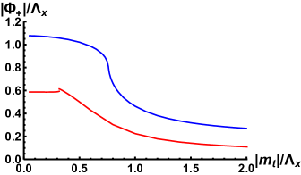
(a) (b)

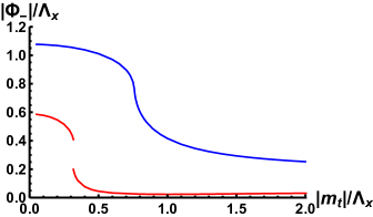
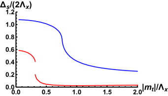
(c) (d)

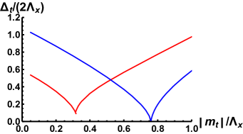
Figure 2: (Color online) Blue curve: we fix $(\lambda,\widetilde{\lambda})=(7,1)$ in Fig. 1 so as to strongly break time-reversal symmetry. Red curve: we fix $(\lambda,\widetilde{\lambda})=4\sqrt{2}(\sin\theta,\cos\theta)$ with $\theta=23\pi/90$ in Fig. 1 so as to weakly break time-reversal symmetry. (a)-(b) Continuous and discontinuous dependence on $m^{\,}_{\mathrm{t}}$ of the stable solution $\Phi^{\,}_{+}$ and $\Phi^{\,}_{-}$ to the saddle point equations (36). (c)-(d) Continuous and discontinuous dependence on $m^{\,}_{\mathrm{t}}$ of the singlet gap $\Delta^{\,}_{\mathrm{s}}$ and the triplet gap $\Delta^{\,}_{\mathrm{t}}$ given by Eq. (38). The triplet gap $\Delta^{\,}_{\mathrm{t}}$ represented by the blue curve vanishes at $|m^{\,}_{\mathrm{t}}|/\Lambda^{\,}_{x}\approx 0.76$ that signals a continuous quantum phase transition.

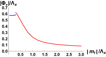
(a) (b)

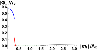
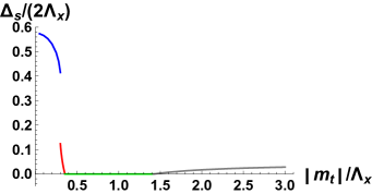
(c) (d)

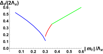
Figure 3: (Color online) (a) and (b) Cut with fixed $\lambda=\widetilde{\lambda}=4$ from Fig. 1(b). The stable mean-field solutions $\Phi^{\,}_{+}$ and $\Phi^{\,}_{-}$ are presented in panels (a) and (b) as functions of $|m^{\,}_{\mathrm{t}}|/\Lambda^{\,}_{x}$, respectively. The $|m^{\,}_{\mathrm{t}}|/\Lambda^{\,}_{x}$ dependence of the singlet ($\Delta^{\,}_{\mathrm{s}}$) and the triplet ($\Delta^{\,}_{\mathrm{t}}$) gaps are plotted in panels (c) and (d) by making use of Eqs. (38a) and (38b), respectively.

III.7 Mean-field phase diagram

By combining Eq. (8) with Eq. (19), we find the singlet and triplet gaps

$$\Delta^{\,}_{\mathrm{s}}\,\raisebox{0.85pt}{.}\raisebox{2.85pt}{.}\!\!=\, \,2\left|\Phi^{\,}_{-}\right|=\left|\phi-\tilde{\phi}\right|,$$ (38a)

$$\Delta^{\,}_{\mathrm{t}}\,\raisebox{0.85pt}{.}\raisebox{2.85pt}{.}\!\!=\, \,2\left||m^{\,}_{\mathrm{t}}|-\left|\Phi^{\,}_{-}\right|\right|=2\left||m^{\,}_{\mathrm{t}}|-\frac{1}{2}\left|\phi-\tilde{\phi}\right|\right|,$$ (38b)

respectively, given a stable solution $(\Phi^{\,}_{+},\Phi^{\,}_{-})$ to the saddle-point equations (36). Correspondingly, we enumerate the following four possibilities

$$\Phi^{\,}_{+}=+\,\Phi^{\,}_{-}=+\phi/2\neq 0,\qquad\tilde{\phi}=0,$$ (39a)

$$\Phi^{\,}_{+}=-\,\Phi^{\,}_{-}=-\tilde{\phi}/2\neq 0,\qquad\phi=0,$$ (39b)

$$\Phi^{\,}_{+}=\phi=\tilde{\phi},\qquad\Phi^{\,}_{-}=0,$$ (39c)

$$\Phi^{\,}_{-}=(\phi-\tilde{\phi})/2=\pm m^{\,}_{\mathrm{t}}\neq 0.$$ (39d)

Case (39a) is obtained when $\lambda>0$ while $\widetilde{\lambda}=0$. Case (39b) is obtained when $\lambda=0$ while $\widetilde{\lambda}\neq 0$. Case (39c) implies that the singlet gap vanishes, $\Delta^{\,}_{\mathrm{s}}=0$, while the triplet gap is solely controlled by the triplet mass, $\Delta^{\,}_{\mathrm{t}}=|m^{\,}_{\mathrm{t}}|$. Case (39d) implies that the triplet gap vanishes, $\Delta^{\,}_{\mathrm{t}}=0$, while the singlet gap is solely controlled by the triplet mass, $\Delta^{\,}_{\mathrm{s}}\neq 2|m^{\,}_{\mathrm{t}}|$.

Figure 1 summarizes the numerical search for the stable solutions to the saddle-point equations (36) in the three-dimensional coupling space $\lambda\geq 0$, $\widetilde{\lambda}\geq 0$, and $|m^{\,}_{\mathrm{t}}|\geq 0$, holding $v^{\,}_{\mu}$ and $m^{\,}_{\mathrm{s}}$ fixed to the values $v^{\,}_{\mu}\equiv 1$ and $m^{\,}_{\mathrm{s}}=0$, respectively. The terminology ATO for Abelian topological order and NATO for non-Abelian topological order applies whenever the stable saddle-point delivers Chern insulating bands with four and one chiral Majorana edge states, respectively, upon imposing open boundary condition along the $y$-direction. Which chirality is to be found on the left ($\mathtt{m}=1$) or right ($\mathtt{m}=n$) ends of the model defined in Eq. (4) is specified by the combination of letters LR or RL. Of course, there is no topological order at the mean-field level as the ground state is non-degenerate when periodic boundary conditions are imposed. However, we conjecture that the ground state manifolds in the ATO and NATO phases acquire distinct non-trivial topological degeneracies when the mean-field approximation is relaxed. Computing these topological degeneracies is beyond the scope of this paper.

III.7.1 Phase transitions between ATO and NATO

There are two wings of yellow-colored surfaces in Fig. 1. Within the same “LR-” or “RL-” topologically ordered phases, ATO and NATO phases are separated by a yellow-colored surface on which the triplet gap $\Delta^{\,}_{\mathrm{t}}$ defined in Eq. (38b) vanishes (namely, $|\Phi^{\,}_{-}|=|m^{\,}_{\mathrm{t}}|$). As a demonstration, we plot in Fig. 2 the blue curves by fixing $(\lambda,\widetilde{\lambda})=(7,1)$ in Fig. 1. In Fig. 2(a)-(b) We find a continuous dependence on $m^{\,}_{\mathrm{t}}$ of the stable solution $\Phi^{\,}_{+}$ and $\Phi^{\,}_{-}$ to the saddle point equations (36). It follows from Eq. (38) that the singlet gap $\Delta^{\,}_{\mathrm{s}}$ and the triplet gap $\Delta^{\,}_{\mathrm{t}}$ in Fig. 2(c)-(d) are also continuous dependent on $m^{\,}_{\mathrm{t}}$. Moreover, the triplet gap vanishes at $|m^{\,}_{\mathrm{t}}|/\Lambda^{\,}_{x}\approx 0.76$ that signals a continuous quantum phase transition.

The two yellow wings to the left and right of the quadrant $\lambda=\tilde{\lambda}$ in Fig. 1 are connected by a stripe (colored in brown) that separates the ATO from the NATO phases by a discontinuous quantum phase transition. As a demonstration, in the red curves of Fig. 2, we move away from $(\lambda,\widetilde{\lambda})=(4,4)$ in Fig. 1 by choosing $(\lambda,\widetilde{\lambda})=4\sqrt{2}(\sin\theta,\cos\theta)$ with $\theta=23\pi/90$. We present the stable solution $\Phi^{\,}_{+}$ and $\Phi^{\,}_{-}$ as a function of $m^{\,}_{\mathrm{t}}$ in the red curves of Fig. 2(a) and (b), respectively. There is a discontinuous dependence on $m^{\,}_{\mathrm{t}}$ of the stable solution $\Phi^{\,}_{+}$ and $\Phi^{\,}_{-}$ to the saddle point equations (36) that delivers a discontinuous dependence on $m^{\,}_{\mathrm{t}}$ of the singlet gap $\Delta^{\,}_{\mathrm{s}}$ and the triplet gap $\Delta^{\,}_{\mathrm{t}}$ in the red curves of Fig. 2(c) and (d).

III.7.2 Case $\lambda=\tilde{\lambda}$

Figure 1(b) summarizes the numerical search for the stable solutions to the saddle-point equations (36) in the quadrant $\lambda=\widetilde{\lambda}\geq 0$, and $|m^{\,}_{\mathrm{t}}|\geq 0$, holding $v^{\,}_{\mu}$ and $m^{\,}_{\mathrm{s}}$ fixed to the values $v^{\,}_{\mu}\equiv 1$ and $m^{\,}_{\mathrm{s}}=0$, respectively. We found three distinct mean-field phases whose boundaries are shown in Fig. 1(b). One phase is gapless. Two phases are gapful when periodic boundary conditions are imposed. The region bounded by the vertical axis and the green curve supports a stable solution to the saddle-point equations (36) with $\Phi^{\,}_{+}\neq 0$ but $\Phi^{\,}_{-}=0$. Hence, this solution respects the time-reversal symmetry of the mean-field Hamiltonian. It follows from Eq. (38) that the triplet gap $\Delta^{\,}_{\mathrm{t}}$ is non-vanishing while the singlet gap $\Delta^{\,}_{\mathrm{s}}$ is vanishing. The triplet of Majorana are thus gapped, while the singlet of Majorana is gapless because of a Dirac-like band touching. The dashed line (colored in brown) in Fig. 1(b) is a line of discontinuous quantum phase transitions by which $|\Phi^{\,}_{-}|<|m^{\,}_{\mathrm{t}}|$ above the dashed line, while $|\Phi^{\,}_{-}|>|m^{\,}_{\mathrm{t}}|$ below the dashed line. The discontinuous jump of $|\Phi^{\,}_{-}|$ is evidence for a mean-field discontinuous quantum phase transition. This discontinuity is mirrored in the discontinuities of $\Phi^{\,}_{+}$, $\Delta^{\,}_{\mathrm{s}}$, and $\Delta^{\,}_{\mathrm{t}}$ as exemplified in Fig. 3 for $(\lambda,\tilde{\lambda})=(4,4).$

As a comparison, we plot in Fig. 4 the stable mean-field solutions $\Phi^{\,}_{+}$ and $\Phi^{\,}_{-}$ as a function of $\theta\,\raisebox{0.85pt}{.}\raisebox{2.85pt}{.}\!\!=\,\mathrm{arctan}(\lambda/\widetilde{\lambda})$ and fixing $\lambda^{2}+\widetilde{\lambda}^{2}=32$ for $|m^{\,}_{\mathrm{t}}|/\Lambda^{\,}_{x}=0.1,1,$ and $3$ in Fig. 4(a),(b) and (c), respectively. When $\theta=\pi/4,$ there is a discontinuous (respectively, continuous) phase transition for panel (a) and (c) [respectively, (b)]. We note that in Fig. 4(a), the value of $|\Phi^{\,}_{-}|$ is not equal to $|\Phi^{\,}_{+}|$ while $||\Phi^{\,}_{+}|-|\Phi^{\,}_{-}||\ll 1$.

(a)

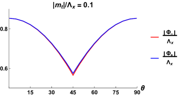
(b)

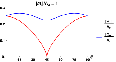
(c)

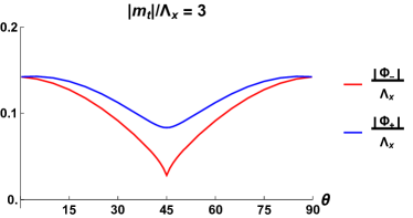
Figure 4: (Color online) The stable mean-field solutions $\Phi^{\,}_{+}$ and $\Phi^{\,}_{-}$ as a function of $\theta:=\mathrm{arctan}(\lambda/\widetilde{\lambda})$ and fixing $\lambda^{2}+\widetilde{\lambda}^{2}=32.$ When $\theta=\pi/4,$ there is a discontinuous (respectively, continuous) phase transition for panel (a) and (c) [respectively, (b)]. (a) Case $|m^{\,}_{\mathrm{t}}|/\Lambda^{\,}_{x}=0.1$. Here, $|\Phi^{\,}_{+}|\neq|\Phi^{\,}_{-}|$ while $||\Phi^{\,}_{+}|-|\Phi^{\,}_{-}||\ll 1$. (b) Case $|m^{\,}_{\mathrm{t}}|/\Lambda^{\,}_{x}=1$. (c) Case $|m^{\,}_{\mathrm{t}}|/\Lambda^{\,}_{x}=3$.

(a)

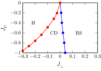
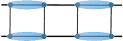
(b) (c)

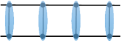
Figure 5: (Color online) (a) The phase diagram for the ladder model (40) as a function of $J^{\,}_{U}<0$ and $|J^{\,}_{\perp}|\leq 0.3.$ The phase boundary between the columnar-dimer (CD) and the rung-singlet (RS) phases is a continuous phase transition in the Ising universality class. The phase boundary between the Haldane phase (H) and the columnar-dimer phase is a continuous phase transition in the $\widehat{su}(2)^{\,}_{2}$ WZNW universality class. (b) Classical representation for the CD order. (c) Classical representation for the RS order.

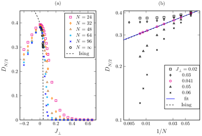
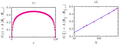
Figure 6: (Color online) (a) Semi-log plot for the leg-dimer order parameter (42) at the center of the ladder, $D^{\,}_{N/2}$, as a function of $J^{\,}_{\perp}$ for different system sizes while fixing $J^{\,}_{U}=-1$. The extrapolation to the thermodynamic limit is obtained with a second-order polynomial in $1/N$, whereas the dashed curve is a fit to the Ising scaling law $D^{\,}_{N/2}\propto N^{-1/8}$. The transition point is at $J^{\,}_{\perp}\approx 0.041$. (b) Fixing $J^{\,}_{U}=-1$, this log-log plot shows the scaling of $D^{\,}_{N/2}$ with $1/N$ for different values of $J^{\,}_{\perp}$ in the vicinity of the critical point. The Ising scaling law fits pretty well the scaling of $D^{\,}_{N/2}$ at the transition point $J^{\,}_{\perp}\approx 0.041$. (c-d) Fitting the entanglement-entropy from Eq. (43) as a function of $x$ with $N=128$ in pane (c) and of $N$ with $x=N/2$ in panel (d) yield $c=0.4692$ and $c=0.4824$, respectively.

IV Lattice regularization

We are going to show that the one-dimensional lattice model (40) regularizes the $(1+1)$-dimensional quantum field theory with the Hamiltonian density obtained by adding Eq. (1) to Eq. (2) with $n=1$. This will be achieved using the density matrix renormalization group (DMRG) White (1992, 1993) to match quantum criticality in the quantum field theory with that in the lattice model.

We will then couple a one-dimensional array of spin-1/2 ladders of the form (40) as is done in Hamiltonian (44) and argue that this two-dimensional lattice model regularizes the Hamiltonian density (4).

IV.1 Numerical study of a two-leg ladder

Following Ref. Chen et al., 2017, we define a spin-1/2 ladder by the Hamiltonian

$$\widehat{H}^{\,}_{\mathrm{ladder}}\,\raisebox{0.85pt}{.}\raisebox{2.85pt}{.}\!\!=\, \,\sum_{i=1}^{N-1}J^{\,}_{1}\,\widehat{\bm{S}}^{\,}_{i}\cdot\widehat{\bm{S}}^{\,}_{i+1}+\sum_{i^{\prime}=1}^{N-1}J^{\,}_{1}\,\widehat{\bm{S}}^{\prime}_{i^{\prime}}\cdot\widehat{\bm{S}}^{\prime}_{i^{\prime}+1}$$

$$\,+\sum_{i=1}^{N}J^{\,}_{\perp}\,\widehat{\bm{S}}^{\,}_{i}\cdot\widehat{\bm{S}}^{\prime}_{i}$$

$$\,+\sum_{i=1}^{N-1}J^{\,}_{\times}\left(\widehat{\bm{S}}^{\,}_{i}\cdot\widehat{\bm{S}}^{\prime}_{i+1}\,+\,\widehat{\bm{S}}^{\,}_{i+1}\cdot\widehat{\bm{S}}^{\prime}_{i}\right)$$

$$\,+\sum_{i=1}^{N-1}J^{\,}_{U}\,\left(\widehat{\bm{S}}^{\,}_{i}\cdot\widehat{\bm{S}}^{\,}_{i+1}\right)\left(\widehat{\bm{S}}^{\prime}_{i}\cdot\widehat{\bm{S}}^{\prime}_{i+1}\right).$$ (40)

Here, $\widehat{\bm{S}}^{\,}_{i}$ and $\widehat{\bm{S}}^{\prime}_{i^{\prime}}$ are spin-1/2 operators localized on the sites of the first and second legs of the ladder, respectively. There are three independent couplings obeying $J^{\,}_{1}>0$ and $J^{\,}_{\perp},J^{\,}_{\times},J^{\,}_{U}\in\mathbb{R}$ with the condition $J^{\,}_{\times}\equiv-J^{\,}_{\perp}/2$. References Shelton et al. (1996); Nersesyan and Tsvelik (1997); Chen et al. (2017) have shown that, at the level of bosonization, the low-energy limit of the ladder (40) is the single copy ($n=1$) of the non-interacting massive Majorana field theory defined by adding the Hamiltonian densities (1) and (2) with the mass terms $m^{\,}_{\mathrm{s}}$ and $m^{\,}_{\mathrm{t}}$ related to the microscopic couplings in Eq. (40) by

$$m^{\,}_{\mathrm{s}}=\frac{-1}{2\pi}\left(12J^{\,}_{\perp}+J^{\,}_{U}\right),\qquad m^{\,}_{\mathrm{t}}=\frac{1}{2\pi}\left(4J^{\,}_{\perp}-J^{\,}_{U}\right).$$ (41)

Bosonization thus predicts the existence for the spin-1/2 ladder (40) of a quantum critical point in the Ising universality class for which $m^{\,}_{\mathrm{s}}=0$ as the dimensionless ratio $J^{\,}_{U}/J^{\,}_{\perp}$ smoothly crosses the critical value $\left(J^{\,}_{U}/J^{\,}_{\perp}\right)^{\,}_{\mathrm{c}}\approx-1/12$. We are going to use the technique of the density matrix renormalization group (DMRG) White (1992, 1993) to verify this prediction. We fix the units of energy by setting $J^{\,}_{1}=1$, bound from above the bond dimension in the DMRG by 1500, and impose open boundary condition.

The phase diagram as a function of $J^{\,}_{U}<0$ and $|J^{\,}_{\perp}|\leq 0.3$ is shown in Fig. 5(a). Here, CD and RS stand for columnar-dimer and rung-singlet, respectively. A classical representation for the CD and the RS phases is obtained by coloring nearest-neighbor bonds as shown in Figs. 5(b) and 5(c). The acronym H stands for the Haldane phase of the antiferromagnetic quantum spin-1 Heisenberg chain Haldane (1983a, b). The Haldane phase is obtained when $J^{\,}_{\perp}$ is ferromagnetic ($J^{\,}_{\perp}<0$) and $|J^{\,}_{U}|$ is not too large. Increasing $|J^{\,}_{U}|$ weakens the Haldane phase until it gives way to the CD phase. Destroying the CD phase is achieved by changing the sign of $J^{\,}_{\perp}$ holding $|J^{\,}_{U}|$ fixed.

The phase boundary between the CD phase and the RS phase is a continuous phase transition belonging to the two-dimensional Ising universality class. The numerical evidence for this Ising transition is supported by the finite-size scaling of the leg-dimer order parameter Lavarélo et al. (2011); Huang et al. (2017)

$$D^{\,}_{i}\,\raisebox{0.85pt}{.}\raisebox{2.85pt}{.}\!\!=\,\left\langle\widehat{\bm{S}}^{\,}_{i}\cdot\left(\widehat{\bm{S}}^{\,}_{i+1}-\widehat{\bm{S}}^{\,}_{i-1}\right)\right\rangle,\quad i=1,\cdots,N-1,$$ (42)

combined with an estimate of the central charge from the scaling of the entanglement entropy.

In Figs. 6(a) and 6(b), we fix $J^{\,}_{U}=-1$. We then calculate $D^{\,}_{N/2}$ for various value of $J^{\,}_{\perp}$. We find an Ising critical point at $J^{\,}_{\perp}\approx 0.041$ for which the Ising scaling law for the order parameter, $D^{\,}_{N/2}\propto N^{-1/8}$, provides an excellent fit.

Another piece of evidence to support the Ising transition is provided by the scaling form of the bipartite von Neumann entanglement entropy under open boundary condition. Calabrese and Cardy (2004, 2009); Laflorencie et al. (2006); Affleck et al. (2009); Cardy and Calabrese (2010); Lavarélo et al. (2011) It is given by

$$S(x,N)=\frac{c}{6}\ln\left(\frac{N+1}{\pi}\sin\frac{\pi\,x}{N+1}\right)+A\langle\widehat{\bm{S}}^{\,}_{x}\cdot\widehat{\bm{S}}^{\,}_{x+1}\rangle+B.$$ (43)

Here, $x$ is the position of the rung at which we partition the ladder into left and right “worlds”, $c$ is the (to be determined) central charge, and $A,B$ are non-universal constants. In Figs. 6(c) and 6(d), we fix $J^{\,}_{U}=-1$ and $J^{\,}_{\perp}=0.041$. In Fig. 6(c), we vary $x$ keeping $N$ fixed. In Fig. 6(d), we fix $x=N/2$ and vary $N$. Both calculations are consistent with an Ising transition for which the exact central charge $c=1/2$.

The phase boundary between the H phase and the RS phase in Fig. 5(a) is predicted within the bosonization framework to be a continuous phase transition belonging to the (1+1)-dimensional $\widehat{su}(2)^{\,}_{2}$ Wess-Zumino-Novikov-Witten (WZNW) universality class. The central charge is $3/2$ and the critical exponent for the scaling of the order parameter is $3/8$. We have obtained DMRG evidence for such a transition in the same way as was done for the Ising transition. As this transition is not the focus of this paper, we will not present these numerical results.

We conclude this section by observing that the spin-ladder model defined in Eq. (40) with $J^{\,}_{\times}\equiv 0$ was recently studied in Ref. Robinson et al., 2018. Reference Robinson et al., 2018 derives a phase diagram similar to that shown in Fig. 5(a). The only differences are the slopes of the phase boundaries. These differences can be understood from the fact that the phase boundaries of the spin-1/2 ladder (40) are determined by the zeros of the masses of the Majorana fields (41). Choosing different intra-ladder couplings changes the relation (41) between the masses of the Majorana fields and the microscopic couplings. This change affects the slopes of the phase boundaries in the microscopic model. We opted to introduce a non-vanishing coupling $J^{\,}_{\times}\equiv-J^{\,}_{\perp}/2$ in Hamiltonian (40) in order to suppress all the bare couplings for all marginally relevant perturbations to the $\widehat{su}(2)_{1}\oplus\widehat{su}(2)_{1}$ WZWN critical point [i.e., all couplings except $J^{\,}_{1}$ set to zero in Eq. (40)]. Shelton et al. (1996); Chen et al. (2017)

IV.2 Model of coupled spin-1/2 two-leg ladders

We take $n$-copies labeled by the index $\mathtt{m}=1,\cdots,n$ of the spin-1/2 ladder (40). We couple this array of spin-1/2 ladders with the inter-ladder interaction Chen et al. (2017)

$$\widehat{H}^{\,}_{\text{inter-ladder}}\,\raisebox{0.85pt}{.}\raisebox{2.85pt}{.}\!\!=\,\widehat{H}^{\,}_{\triangle}+\widehat{H}^{\prime}_{\triangle}+\widehat{H}^{\,}_{\square}+\widehat{H}^{\prime}_{\square},$$ (44a)

where

$$\widehat{H}^{\,}_{\triangle}\,\raisebox{0.85pt}{.}\raisebox{2.85pt}{.}\!\!=\, \,\frac{J^{\,}_{\chi}}{2}\,\sum_{i=1}^{N}\sum_{\mathtt{m}=1}^{n-1}\Big{[}\widehat{\bm{S}}^{\,}_{i,\mathtt{m}+1}\cdot\left(\widehat{\bm{S}}^{\,}_{i+1,\mathtt{m}}\wedge\widehat{\bm{S}}^{\,}_{i,\mathtt{m}}\right)$$

$$\,+\widehat{\bm{S}}^{\,}_{i+1,\mathtt{m}}\cdot\left(\widehat{\bm{S}}^{\,}_{i,\mathtt{m}+1}\wedge\widehat{\bm{S}}^{\,}_{i+1,\mathtt{m}+1}\right)\Big{]}$$ (44b)

and

$$\widehat{H}^{\,}_{\square}\,\raisebox{0.85pt}{.}\raisebox{2.85pt}{.}\!\!=\, \,J^{\,}_{\vee}\,\sum_{i=1}^{N}\sum_{\mathtt{m}=1}^{n-1}\Big{(}\widehat{\bm{S}}^{\,}_{i,\mathtt{m}}\cdot\widehat{\bm{S}}^{\,}_{i,\mathtt{m}+1}$$

$$\,+\frac{1}{2}\widehat{\bm{S}}^{\,}_{i,\mathtt{m}+1}\cdot\widehat{\bm{S}}^{\,}_{i+1,\mathtt{m}}+\frac{1}{2}\widehat{\bm{S}}^{\,}_{i,\mathtt{m}}\cdot\widehat{\bm{S}}^{\,}_{i+1,\mathtt{m}+1}\Big{)},$$ (44c)

with $\widehat{H}^{\prime}_{\triangle}$ and $\widehat{H}^{\prime}_{\square}$ deduced from $\widehat{H}^{\,}_{\triangle}$ and $\widehat{H}^{\,}_{\square}$ by the substitution $\widehat{\bm{S}}^{\,}_{i,\mathtt{m}}\to\widehat{\bm{S}}^{\prime}_{i,\mathtt{m}}$. The low energy limit of Hamiltonian $\widehat{H}^{\,}_{\text{inter-ladder}}$ was obtained using bosonization in Ref. Huang et al., 2017; Chen et al., 2017 (see also Ref. Gorohovsky et al., 2015). Aside from a renormalization of the velocities entering the quadratic Hamiltonian density (1), it produces, as was shown in Ref. Tsvelik, 1990, the quartic Majorana interaction (3) with the couplings $\lambda$ and $\widetilde{\lambda}$ related to the microscopic couplings entering Eq. (44b) by Huang et al. (2017); Chen et al. (2017)

$$\lambda=2\mathfrak{a}\left[(J^{\,}_{\chi}/\pi)+2J^{\,}_{\vee}\right],\quad\widetilde{\lambda}=2\mathfrak{a}\left[-(J^{\,}_{\chi}/\pi)+2J^{\,}_{\vee}\right].$$ (45a)

We will use shortly the reciprocal relation

$$J^{\,}_{\vee}=\frac{1}{8\mathfrak{a}}\left(\lambda+\widetilde{\lambda}\right),\quad J^{\,}_{\chi}=\frac{\pi}{4\mathfrak{a}}\left(\lambda-\widetilde{\lambda}\right).$$ (45b)

The two-dimensional spin-1/2 model is then defined by

$$\widehat{H}\,\raisebox{0.85pt}{.}\raisebox{2.85pt}{.}\!\!=\,\widehat{H}^{\mathrm{array}}_{\mathrm{ladder}}+\widehat{H}^{\,}_{\text{inter-ladder}},$$ (46)

where $\widehat{H}^{\mathrm{array}}_{\mathrm{ladder}}$ is simply the sum of $n$ copies of the spin-1/2 ladder (40).

IV.3 Implications

We are now ready to deduce from the mean-field phase diagram Fig. 1 of the quantum field theory (4) the following predictions for the two-dimensional array of coupled spin-1/2 ladders (46).

First, fixing $m^{\,}_{\mathrm{s}}=0$ implies the linear condition [c.f. Eq. (41)]

$$J^{\,}_{\perp}\propto-J^{\,}_{U}.$$ (47)

It then follows that $m^{\,}_{\mathrm{t}}$ is only controlled by one parameter, namely

$$|m^{\,}_{\mathrm{t}}|\propto|J^{\,}_{\perp}|\propto|J^{\,}_{U}|.$$ (48)

Second, fixing $\lambda=\widetilde{\lambda}$ implies $J^{\,}_{\chi}\equiv 0$, i.e., the three-spin interaction that breaks explicitly time-reversal symmetry must vanish. We then deduce from the quantum field theory (4) that the two-dimensional spin-1/2 lattice model (46) could support three phases, of which two are gapped and break spontaneously the time-reversal symmetry while one is gapless and time-reversal symmetric. There is an important a caveat here, namely that we have neglected perturbations, whose bare couplings are very small (e.g., generated by quantum corrections) but relevant at the $\bigoplus_{\mathtt{m}}[\widehat{su}(2)_{1}\oplus\widehat{su}(2)^{\,}_{1}]$ WZWN critical point, that would stabilize collinear long-ranged ordered phase or dimer phases.Starykh and Balents (2004, 2007) If we ignore this possibility, a too small or too large $|m^{\,}_{\mathrm{t}}|\propto|J^{\,}_{\perp}|\propto|J^{\,}_{U}|$ could then stabilize a topologically ordered spin-liquid phase, whereas intermediate values of $|m^{\,}_{\mathrm{t}}|\propto|J^{\,}_{\perp}|\propto|J^{\,}_{U}|$ with $\lambda=\widetilde{\lambda}\propto~{}J^{\,}_{\vee}>0$ not too large (say, $\lambda\lesssim 8$) could stabilize a gapless spin-liquid phase with a Dirac point. The mean-field transition through the time-reversal-symmetric quadrant $\lambda=\widetilde{\lambda}$ from the region with $\lambda<\widetilde{\lambda}$ to the region with $\lambda>\widetilde{\lambda}$ is continuous (discontinuous) if it goes through the gapless (one of the gapped) phase.

V Summary

We have studied a strongly interacting quantum field theory (QFT) describing a two-dimensional array of wires containing four (a singlet and a triplet) massive Majorana fields in $(1+1)$-dimensional spacetime. This QFT is a continuum limit of a two-dimensional lattice model of spins S=1/2 interacting via SU(2) symmetric two- three- and four spin interactions. In the continuum limit these interactions give rise to two Majorana masses and to competing quartic Majorana interactions (with couplings $\lambda$ and $\widetilde{\lambda}$) that are interchanged under time reversal. The case $\lambda\neq 0$, $\widetilde{\lambda}=0$ when the time reversal is explicitly broken was studied by us before Chen et al. (2017). Here, we have considered the limit $\lambda=\widetilde{\lambda}$ and established the conditions under which time-reversal symmetry is broken spontaneously.

At the mean-field level on the time-reversal-symmetric plane $\lambda=\widetilde{\lambda}$. we have found three competing phases. There are two gapped phases that break spontaneously the time-reversal symmetry, They are gapped in the bulk, and support chiral Majorana edge modes carrying the chiral central charges 2 and 1/2, respectively. One phase is conjectured to signal an Abelian topological order (ATO), the other is conjectured to signal a non-Abelian topological order (NATO), if the mean-field approximation is relaxed. This pair of mean-field gapped phases is separated by a line of points at which a discontinuous phase transition takes place. However, we have also found a time-reversal-symmetric mean-field phase that supports a branch of mean-field Majorana modes with a gapless Dirac spectrum. This phase is bounded by a line of continuous phase transitions separating it from the mean-field snapshot of the NATO phase.

We remark that although we have assumed that the singlet mass $m^{\,}_{\mathrm{s}}$ is vanishing in our mean-field analysis and treated the triplet mass $m^{\,}_{\mathrm{t}}$ as a tunable parameter, we could equally well have reversed the roles of the singlet and triplet masses. If so, we can simply exchange the role played by the triplet and the singlet Majorana modes. The resulting mean-field phase diagram would contain again the mean-field snapshots of an Abelian phase and of a non-Abelian phase. The Abelian phase is the same Abelian phase as in the present study. The non-Abelian phase would be different, however, as its chiral edge modes would carry a chiral central charge of $3/2$. A non-Abelian topologically ordered phase with chiral edge states endowed with the central charge $3/2$ is a cousin to the Moore-Read state for the fractional quantum Hall effect Moore and Read (1991). One also finds such a non-Abelian topologically ordered phase for certain spin-$1$ Heisenberg models on the square lattice Chen et al. (2018).

References

• Kalmeyer and Laughlin (1987) V. Kalmeyer and R. B. Laughlin, “Equivalence of the resonating-valence-bond and fractional quantum Hall states,” Phys. Rev. Lett. 59, 2095 (1987).
• Wen (1991) Xiao-Gang Wen, “Topological orders and chern-simons theory in strongly correlated quantum liquid,” Int. J. Mod. Phys. B 05, 1641 (1991).
• Kitaev (2006) Alexei Kitaev, “Anyons in an exactly solved model and beyond,” Annals of Physics 321, 2 (2006).
• Moore and Read (1991) Gregory Moore and Nicholas Read, “Nonabelions in the fractional quantum hall effect,” Nucl. Phys. B360, 362 (1991).
• Mukhopadhyay et al. (2001) Ranjan Mukhopadhyay, C. L. Kane,  and T. C. Lubensky, “Crossed sliding luttinger liquid phase,” Phys. Rev. B 63, 081103 (2001).
• Kane et al. (2002) C. L. Kane, Ranjan Mukhopadhyay,  and T. C. Lubensky, “Fractional quantum hall effect in an array of quantum wires,” Phys. Rev. Lett. 88, 036401 (2002).
• Teo and Kane (2014) Jeffrey C. Y. Teo and C. L. Kane, “From luttinger liquid to non-abelian quantum hall states,” Phys. Rev. B 89, 085101 (2014).
• Kane et al. (2017) Charles L. Kane, Ady Stern,  and Bertrand I. Halperin, “Pairing in luttinger liquids and quantum hall states,” Phys. Rev. X 7, 031009 (2017).
• Kane and Stern (2018) Charles L. Kane and Ady Stern, “Coupled wire model of ${Z}_{4}$ orbifold quantum hall states,” Phys. Rev. B 98, 085302 (2018).
• Wen (1990) X. G. Wen, “Chiral luttinger liquid and the edge excitations in the fractional quantum hall states,” Phys. Rev. B 41, 12838 (1990).
• Gorohovsky et al. (2015) Gregory Gorohovsky, Rodrigo G. Pereira,  and Eran Sela, “Chiral spin liquids in arrays of spin chains,” Phys. Rev. B 91, 245139 (2015).
• Huang et al. (2016) Po-Hao Huang, Jyong-Hao Chen, Pedro R. S. Gomes, Titus Neupert, Claudio Chamon,  and Christopher Mudry, “Non-abelian topological spin liquids from arrays of quantum wires or spin chains,” Phys. Rev. B 93, 205123 (2016).
• Lecheminant and Tsvelik (2017) P. Lecheminant and A. M. Tsvelik, “Lattice spin models for non-abelian chiral spin liquids,” Phys. Rev. B 95, 140406 (2017).
• Huang et al. (2017) Po-Hao Huang, Jyong-Hao Chen, Adrian E. Feiguin, Claudio Chamon,  and Christopher Mudry, “Coupled spin-$\frac{1}{2}$ ladders as microscopic models for non-abelian chiral spin liquids,” Phys. Rev. B 95, 144413 (2017).
• Chen et al. (2017) Jyong-Hao Chen, Christopher Mudry, Claudio Chamon,  and A. M. Tsvelik, “Model of chiral spin liquids with abelian and non-abelian topological phases,” Phys. Rev. B 96, 224420 (2017).
• Pereira and Bieri (2018) Rodrigo G. Pereira and Samuel Bieri, “Gapless chiral spin liquid from coupled chains on the kagome lattice,” SciPost Phys. 4, 004 (2018).
• Wen et al. (1989) X. G. Wen, F. Wilczek,  and A. Zee, “Chiral spin states and superconductivity,” Phys. Rev. B 39, 11413 (1989).
• Assaad and Grover (2016) F. F. Assaad and Tarun Grover, “Simple fermionic model of deconfined phases and phase transitions,” Phys. Rev. X 6, 041049 (2016).
• Haldane (1988) F. D. M. Haldane, “Model for a quantum hall effect without landau levels: Condensed-matter realization of the ”parity anomaly”,” Phys. Rev. Lett. 61, 2015 (1988).
• Note (1) In Eq. (31b), the integral over $\omega$ can be carried out by using the following formula for definite integral Stone (2000)
\ilimits@dω2πln(ω2+k2+A2)=k2+A2+const,subscriptsuperscript\ilimits@d𝜔2𝜋𝑙𝑛superscript𝜔2superscript𝑘2superscript𝐴2superscript𝑘2superscript𝐴2const\intop\ilimits@\limits^{\infty}_{-\infty}\frac{\mathrm{d}\omega}{2\pi}\mathop{ln}\nolimits\left(\omega^{2}+k^{2}+A^{2}\right)=\sqrt{k^{2}+A^{2}}+\mathrm{const},
where the constant is formally infinity.
• White (1992) Steven R. White, “Density matrix formulation for quantum renormalization groups,” Phys. Rev. Lett. 69, 2863 (1992).
• White (1993) Steven R. White, “Density-matrix algorithms for quantum renormalization groups,” Phys. Rev. B 48, 10345 (1993).
• Shelton et al. (1996) D. G. Shelton, A. A. Nersesyan,  and A. M. Tsvelik, “Antiferromagnetic spin ladders: Crossover between spin S =1/2 and S =1 chains,” Phys. Rev. B 53, 8521 (1996).
• Nersesyan and Tsvelik (1997) A. A. Nersesyan and A. M. Tsvelik, “One-dimensional spin-liquid without magnon excitations,” Phys. Rev. Lett. 78, 3939 (1997).
• Haldane (1983a) F.D.M. Haldane, “Continuum dynamics of the 1-d heisenberg antiferromagnet: Identification with the o(3) nonlinear sigma model,” Phys. Lett. A93, 464 (1983a).
• Haldane (1983b) F. D. M. Haldane, “Nonlinear field theory of large-spin heisenberg antiferromagnets: Semiclassically quantized solitons of the one-dimensional easy-axis néel state,” Phys. Rev. Lett. 50, 1153 (1983b).
• Lavarélo et al. (2011) Arthur Lavarélo, Guillaume Roux,  and Nicolas Laflorencie, “Melting of a frustration-induced dimer crystal and incommensurability in the ${J}_{1}$-${J}_{2}$ two-leg ladder,” Phys. Rev. B 84, 144407 (2011).
• Calabrese and Cardy (2004) Pasquale Calabrese and John Cardy, “Entanglement entropy and quantum field theory,” J. Stat. Mech. (2004) P06002 2004, P06002 (2004).
• Calabrese and Cardy (2009) Pasquale Calabrese and John Cardy, “Entanglement entropy and conformal field theory,” J. Phys. A 42, 504005 (2009).
• Laflorencie et al. (2006) Nicolas Laflorencie, Erik S. Sørensen, Ming-Shyang Chang,  and Ian Affleck, “Boundary effects in the critical scaling of entanglement entropy in 1d systems,” Phys. Rev. Lett. 96, 100603 (2006).
• Affleck et al. (2009) Ian Affleck, Nicolas Laflorencie,  and Erik S. Sørensen, “Entanglement entropy in quantum impurity systems and systems with boundaries,” J. Phys. A 42, 504009 (2009).
• Cardy and Calabrese (2010) John Cardy and Pasquale Calabrese, “Unusual corrections to scaling in entanglement entropy,” J. Stat. Mech. (2010) P04023 2010, P04023 (2010).
• Robinson et al. (2018) N. J. Robinson, A. Altland, R. Egger, N. M. Gergs, W. Li, D. Schuricht, A. M. Tsvelik, A. Weichselbaum,  and R. M. Konik, “Non-Topological Majorana Zero Modes in Inhomogeneous Spin Ladders,” ArXiv e-prints  (2018), arXiv:1806.01925 [cond-mat.str-el] .
• Tsvelik (1990) A. M. Tsvelik, “Field-theory treatment of the heisenberg spin-1 chain,” Phys. Rev. B 42, 10499 (1990).
• Starykh and Balents (2004) Oleg A. Starykh and Leon Balents, “Dimerized phase and transitions in a spatially anisotropic square lattice antiferromagnet,” Phys. Rev. Lett. 93, 127202 (2004).
• Starykh and Balents (2007) Oleg A. Starykh and Leon Balents, “Ordering in spatially anisotropic triangular antiferromagnets,” Phys. Rev. Lett. 98, 077205 (2007).
• Chen et al. (2018) J.-Y. Chen, L. Vanderstraeten, S. Capponi,  and D. Poilblanc, “Non-Abelian chiral spin liquid in a quantum antiferromagnet revealed by an iPEPS study,” ArXiv e-prints  (2018), arXiv:1807.04385 [cond-mat.str-el] .
• Note (2) ITensor library (version 2.1.1) http://itensor.org.
• Stone (2000) Michael Stone, The physics of quantum fields (Springer, New York, 2000).