Infinite-dimensional meta-conformal Lie algebras in one and two spatial dimensions

Malte Henkel^a,b and Stoimen Stoimenov^c

^a Laboratoire de Physique et Chimie Théoriques (CNRS UMR 7019), Université de Lorraine Nancy,

B.P. 70239, F – 54506 Vandœuvre lès Nancy Cedex, France

^b Centro de Física Teórica e Computacional, Universidade de Lisboa, P – 1749-016 Lisboa, Portugal

^c Institute of Nuclear Research and Nuclear Energy, Bulgarian Academy of Sciences,

72 Tsarigradsko chaussee, Blvd., BG – 1784 Sofia, Bulgaria

Meta-conformal transformations are constructed as sets of time-space transformations which are not angle-preserving but contain time- and space translations, time-space dilatations with dynamical exponent $\mathpzc{z}=1$ and whose Lie algebras contain conformal Lie algebras as sub-algebras. They act as dynamical symmetries of the linear transport equation in $d$ spatial dimensions. For $d=1$ spatial dimensions, meta-conformal transformations constitute new representations of the conformal Lie algebras, while for $d\neq 1$ their algebraic structure is different. Infinite-dimensional Lie algebras of meta-conformal transformations are explicitly constructed for $d=1$ and $d=2$ and they are shown to be isomorphic to the direct sum of either two or three centre-less Virasoro algebras, respectively. The form of co-variant two-point correlators is derived. An application to the directed Glauber-Ising chain with spatially long-ranged initial conditions is described.

“Whenever you have to do with a structure-endowed entity, try to determine its group of automorphisms. You can expect to gain a deep insight.”
  H. Weyl, Symmetry, Princeton University Press (1952)

1 Introduction

Conformal invariance has found many brilliant applications, for example to string theory and high-energy physics [79], or to two-dimensional phase transitions [11, 37, 54, 81] the quantum Hall effect [20, 50], or certain stochastic processes [2, 3, 4, 27, 71, 82]. These applications are based on a geometric definition of conformal transformations, considered as local coordinate transformations $\bm{r}\mapsto\bm{r}^{\prime}=\bm{f}(\bm{r})$, of spatial coordinates $\bm{r}\in\mathbb{R}^{2}$ such that angles are kept unchanged. The Lie algebra of these transformations is naturally called the ‘conformal Lie algebra’.

1. In order to establish our notation, we briefly recall some basic facts, concentrating on $d=2$. Use complex light-cone coordinates $z=t+{\rm i}\mu r$ and $\bar{z}=t-{\rm i}\mu r$, where the ‘time’ $t$ and the ‘space’ $r$ label the two directions, and $\mu$ is an universal constant with the units of an inverse velocity. The Lie algebra generators read, for $n\in\mathbb{Z}$

$$\ell_{n}=-z^{n+1}\partial_{z}-(n+1)\Delta z^{n}\>\;,\;\;\bar{\ell}_{n}=-\bar{z}^{n+1}\partial_{\bar{z}}-(n+1)\overline{\Delta}\bar{z}^{n}$$ (1.1)

where $\Delta=\frac{1}{2}(\delta-{\rm i}\gamma/\mu)$, $\overline{\Delta}=\frac{1}{2}(\delta+{\rm i}\gamma/\mu)$ are the conformal weights of the scaling operators on which these generators act. The generators (1.1) obey the commutation relations of $\mathfrak{vect}(S^{1})\oplus\mathfrak{vect}(S^{1})$

$$\left[\ell_{n},\ell_{m}\right]=(n-m)\ell_{n+m}\;\;,\;\;\left[\ell_{n},\bar{\ell}_{m}\right]=0\;\;,\;\;\left[\bar{\ell}_{n},\bar{\ell}_{m}\right]=(n-m)\bar{\ell}_{n+m}$$ (1.2)

The maximal finite-dimensional Lie sub-algebra is $\mathfrak{conf}(2):=\left\langle\ell_{\pm 1,0},\bar{\ell}_{\pm 1,0}\right\rangle\cong\mathfrak{sl}(2,\mathbb{R})\oplus\mathfrak{sl}(2,\mathbb{R})$. For what follows, we rather consider the generators $X_{n}:=\ell_{n}+\bar{\ell}_{n}$ and $Y_{n}:={\rm i}\mu\bigl{(}\ell_{n}-\bar{\ell}_{n}\bigr{)}$ which in ‘time’ and ‘space’ coordinates read

$$X_{n} = -\frac{1}{2}\left[(t+{\rm i}\mu r)^{n+1}+(t-{\rm i}\mu r)^{n+1}\right]\partial_{t}+\frac{{\rm i}}{2\mu}\left[(t+{\rm i}\mu r)^{n+1}-(t-{\rm i}\mu r)^{n+1}\right]\partial_{r}$$

$$-\frac{n+1}{2}\delta\left[(t+{\rm i}\mu r)^{n}+(t-{\rm i}\mu r)^{n}\right]-\frac{n+1}{2}\frac{\gamma}{{\rm i}\mu}\left[(t+{\rm i}\mu r)^{n}-(t-{\rm i}\mu r)^{n}\right]$$

$$Y_{n} = -\frac{{\rm i}\mu}{2}\left[(t+{\rm i}\mu r)^{n+1}-(t-{\rm i}\mu r)^{n+1}\right]\partial_{t}-\frac{1}{2}\left[(t+{\rm i}\mu r)^{n+1}+(t-{\rm i}\mu r)^{n+1}\right]\partial_{r}$$ (1.3)

$$-\frac{n+1}{2}{\rm i}\mu\delta\left[(t+{\rm i}\mu r)^{n}-(t-{\rm i}\mu r)^{n}\right]-\frac{n+1}{2}\gamma\left[(t+{\rm i}\mu r)^{n}+(t-{\rm i}\mu r)^{n}\right]$$

Herein, $\delta$ and $\gamma$ denote the scaling dimension and the (rescaled) spin of the respective scaling operator. The commutators (1.2) are recast into

$$\left[X_{n},X_{m}\right]=(n-m)X_{n+m}\;\;,\;\;\left[X_{n},Y_{m}\right]=(n-m)Y_{n+m}\;\;,\;\;\left[Y_{n},Y_{m}\right]=-\mu\,(n-m)X_{n+m}$$ (1.4)

These conformal transformations also act as dynamical symmetries of differential equations. ‘Dynamical symmetry’ means throughout [77] that the space of solutions of the equation $\hat{\mathscr{S}}\phi=0$ is invariant under the conformal transformations (1.1). The most simple example is the Laplace equation $\hat{\mathscr{S}}\phi=0$, where $\phi=\phi(z,\bar{z})=\varphi(t,r)$ and

$$\hat{\mathscr{S}}=4\mu^{2}\partial_{z}\partial_{\bar{z}}=\mu^{2}\partial_{t}^{2}+\partial_{r}^{2}$$ (1.5)

The dynamical conformal symmetry of (1.5) follows from the commutators

$$\left[\hat{\mathscr{S}},\ell_{n}\right] = -(n+1)z^{n}\hat{\mathscr{S}}-4n(n+1)\mu^{2}\Delta z^{n-1}\partial_{\bar{z}}$$

$$\left[\hat{\mathscr{S}},\bar{\ell}_{n}\right] = -(n+1)\bar{z}^{n}\hat{\mathscr{S}}-4n(n+1)\mu^{2}\overline{\Delta}\bar{z}^{n-1}\partial_{z}$$ (1.6)

and provided that $\Delta=\overline{\Delta}=0$. Of course, the physical interest in conformal invariance comes from the multitude of systems, beyond the Laplace equation and which are conformally invariant, as mentioned above. Finally, the requirement of co-variance under conformal transformations is sufficient to fix certain $n$-point functions of the scaling operators $\phi_{i}(z_{i},\bar{z}_{i})$. For example, the two-point function $C(z,\bar{z})=C(t,r)$ reads, up to normalisation

$$C(z,\bar{z}) = \left\langle\phi_{1}(z,\bar{z})\phi_{2}(0,0)\right\rangle\>=\>\delta_{\Delta_{1},\Delta_{2}}\delta_{\overline{\Delta}_{1},\overline{\Delta}_{2}}\>z^{-2\Delta_{1}}\bar{z}^{-2\overline{\Delta}_{1}}$$ (1.7)

$$= \left\langle\varphi_{1}(t,r)\varphi_{2}(0,0)\right\rangle\>=\>\delta_{\delta_{1},\delta_{2}}\delta_{\gamma_{1},\gamma_{2}}\,\left(t^{2}+\mu^{2}r^{2}\right)^{-\delta_{1}}\exp\left(-\frac{2\gamma_{1}}{\mu}\arctan\left(\mu\frac{r}{t}\right)\right)~{}~{}~{}~{}$$

2. Are there other groups of time-space transformations which can act as dynamical symmetries in certain physical situations ? In table 1, several examples of infinite-dimensional Lie groups of time-space transformations are listed. The Schrödinger-Virasoro group [52, 56, 88] is distinct from the conformal group in that the dilatations are of the form $t\mapsto b^{\mathpzc{z}}t$ and $\bm{r}\mapsto b\bm{r}$, with the dynamical exponent $\mathpzc{z}=2$ for the Schrödinger group, in contrast to $\mathpzc{z}=1$ for the conformal group. Its maximal finite-dimensional subgroup is the Schrödinger group [69, 73, 77, 15, 48, 68], which acts as dynamical symmetry on the free diffusion/Schrödinger equation. Schrödinger-covariance predicts the form of response functions, as they arise for example in phase-ordering kinetics, notably in non-equilibrium $2D$ and $3D$ Ising and Potts models, whose dynamics are not described by free-field theories. See [58] for a review and [65] for a tutorial introduction.

group	coordinate changes			co-variance
ortho-conformal $(1+1)D$	$z^{\prime}=f(z)$	$\bar{z}^{\prime}=\bar{z}$		correlator
	$z^{\prime}=z$	$\bar{z}^{\prime}=\bar{f}(\bar{z})$
Schrödinger-Virasoro	$t^{\prime}=b(t)$	$\bm{r}^{\prime}=\left({\rm d}b(t)/{\rm d}t\right)^{1/2}\bm{r}$		response
	$t^{\prime}=t$	$\bm{r}^{\prime}=\bm{r}+\bm{a}(t)$
	$t^{\prime}=t$	$\bm{r}^{\prime}=\mathscr{R}(t)\bm{r}$
conformal galilean	$t^{\prime}=b(t)$	$\bm{r}^{\prime}=\left({\rm d}b(t)/{\rm d}t\right)\bm{r}$		correlator
	$t^{\prime}=t$	$\bm{r}^{\prime}=\bm{r}+\bm{a}(t)$
	$t^{\prime}=t$	$\bm{r}^{\prime}=\mathscr{R}(t)\bm{r}$
meta-conformal $1D$	$u=f(u)$	$\bar{u}^{\prime}=\bar{u}$		correlator
	$u^{\prime}=u$	$\bar{u}^{\prime}=\bar{f}(\bar{u})$
meta-conformal $2D$	$\tau^{\prime}=\tau$	$w^{\prime}=f(w)$	$\bar{w}^{\prime}=\bar{w}$
	$\tau^{\prime}=\tau$	$w^{\prime}=w$	$\bar{w}^{\prime}=\bar{f}(\bar{w})$
	$\tau^{\prime}=b(\tau)$	$w^{\prime}=w$	$\bar{w}^{\prime}=\bar{w}$

Table 1: Examples of infinite-dimensional groups of time-space transformations, with the defining coordinate changes. Herein, $f,\bar{f},b,\bm{a}$ are arbitrary differentiable (vector) functions of their argument and $\mathscr{R}(t)\in\mbox{\sl SO}(d)$ is a time-dependent rotation matrix. Physical interpretations of the coordinates $(u,\bar{u})$ and $(\tau,w,\bar{w})$ of the $1D$ and $2D$ meta-conformal transformations are listed in tables 2 and 3. The physical interpretation of the co-variant $n$-point functions as either correlators or responses is based on the extension of the Cartan sub-algebra [59, 60, 62].

If we concentrate on systems with a dynamical exponent $\mathpzc{z}=1$, can one find infinite-dimensional groups of time-space transformations distinct from the conformal transformations reviewed above ? For the sake of a clear conceptual distinction, those standard conformal transformations, generated from (1.1) or (1.3), will from now on be called ‘ortho-conformal’. It will turn out that alternative sets of time-space transformations exist. In contrast to ortho-conformal transformations, these new transformations are not angle-preserving, neither in a space made from time-space points $(t,\bm{r})\in\mathbb{R}^{1+d}$, nor in space with points $(\bm{r})\in\mathbb{R}^{d}$. On the other hand, their Lie algebras still contain ortho-conformal Lie algebras as sub-algebras. We shall therefore call them ‘meta-conformal transformations’ [63, 64].

3. In a two-dimensional time-space with points $(t,r)\in\mathbb{R}^{2}$, meta-conformal transformations have the infinitesimal generators [55]

$$X_{n} = -t^{n+1}\partial_{t}-\mu^{-1}[(t+\mu r)^{n+1}-t^{n+1}]\partial_{r}-(n+1)\frac{\gamma}{\mu}[(t+\mu r)^{n}-t^{n}]-(n+1)\delta t^{n}$$

$$Y_{n} = -(t+\mu r)^{n+1}\partial_{r}-(n+1)\gamma(t+\mu r)^{n}$$ (1.8)

where $\delta,\gamma$ are constants and $\mu^{-1}$ is a constant universal velocity (‘speed of sound’ or ‘speed of light’). The generators $X_{-1}=-\partial_{t}$ and $Y_{-1}=-\partial_{r}$ of time- and space-translations, as well as the generator $X_{0}=-t\partial_{t}-r\partial_{r}-\delta$ of dilatations are the same as for ortho-conformal transformations (1.3). The other generators are different and the generators (1.8) are in general not angle-preserving. Their Lie algebra $\langle X_{n},Y_{n}\rangle_{n\in\mathbb{Z}}$ obeys

$$[X_{n},X_{m}]=(n-m)X_{n+m},\quad[X_{n},Y_{m}]=(n-m)Y_{n+m},\quad[Y_{n},Y_{m}]=\mu(n-m)Y_{n+m}$$ (1.9)

The maximal finite-dimensional Lie sub-algebra is denoted $\mathfrak{meta}(1,1):=\left\langle X_{\pm 1,0},Y_{\pm 1,0}\right\rangle$. Indeed, if $\mu\neq 0$, (1.9) is isomorphic to the Lie algebra (1.4). To see this, let $X_{n}=\ell_{n}+\bar{\ell}_{n}$ and $Y_{n}=\mu\bar{\ell}_{n}$. This gives

$$\ell_{n} = -t^{n+1}\left(\partial_{t}-\frac{1}{\mu}\partial_{r}\right)-(n+1)\left(\delta-\frac{\gamma}{\mu}\right)t^{n}$$

$$\bar{\ell}_{n} = -\frac{1}{\mu}(t+\mu r)^{n+1}\partial_{r}-(n+1)\frac{\gamma}{\mu}(t+\mu r)^{n}.$$ (1.10)

which again satisfy the commutators (1.2). The reduction of (1.10) to the standard form (1.1) in ‘complex’ light-cone coordinates $z,\bar{z}$ is achieved by setting $z=t$ and $\bar{z}=t+\mu r$, and identifying the conformal weights $\Delta=\delta-\gamma/\mu$ and $\overline{\Delta}=\gamma/\mu$. In $1+1$ time-space dimensions, the meta-conformal transformations (1.8) and the ortho-conformal transformations (1.4) are two representations of the same conformal Lie algebra, see also table 1.

The meta-conformal generators (1.8) are dynamical symmetries of the equation of motion

$$\hat{\mathscr{S}}\phi(t,r)=(-\mu\partial_{t}+\partial_{r})\varphi(t,r)=0.$$ (1.11)

Indeed, since (with $n\in\mathbb{Z}$)

$${}[\hat{\mathscr{S}},X_{n}]=-(n+1)t^{n}\hat{\mathscr{S}}+n(n+1)\mu\left(\delta-\frac{\gamma}{\mu}\right)t^{n-1}\;\;,\;\;{}[\hat{\mathscr{S}},Y_{n}]=0$$ (1.12)

a solution $\varphi$ of (1.11) with scaling dimension $\delta_{\varphi}=\delta=\gamma/\mu$ is mapped onto another solution of (1.11). Hence the space of solutions of the equation (1.11) is meta-conformally invariant. This is the analogue of the ortho-conformal invariance of the $2D$ Laplace equation. This kind of equation of motion (1.11), with a directional bias, motivates to look for physical applications in the kinetics of spin systems with directed dynamics, as we shall do in section 5.

Meta-conformally co-variant two-point functions have the form [58], up to normalisation

$$C(t,r)=\left\langle\varphi_{1}(t,r)\varphi_{2}(0,0)\right\rangle=\delta_{\delta_{1},\delta_{2}}\delta_{\gamma_{1},\gamma_{2}}\>t^{-2\delta_{1}}\left(1+\frac{\gamma_{1}}{\mu}\frac{r}{t}\right)^{-2\gamma_{1}/\mu}$$ (1.13)

4. In the limit $\mu\to 0$, for both ortho-conformal as well as for meta-conformal transformations, one can make a Lie algebra contraction of (1.4) or (1.9). The result is called ‘conformal galilean algebra’ $\mbox{\sc cga}(1)$ [51] or ‘bms-algebra’ $\mathfrak{bms}_{3}$[14]. Table 1 give the time-space transformations which follow from $\mbox{\sc cga}(d)$ for $d\geq 1$ (rotations by arbitrary time-dependent angles appear for $d\geq 2$). The generators of $\mbox{\sc cga}(1)$ can be read off by taking the limit $\mu\to 0$ in either (1.3) or else in (1.8). Taking the limit $\mu\to 0$ in either (1.7) or else (1.13) gives the $\mbox{\sc cga}(1)$-covariant two-point function

$$C(t,r)=\left\langle\varphi_{1}(t,r)\varphi_{2}(0,0)\right\rangle=\delta_{\delta_{1},\delta_{2}}\delta_{\gamma_{1},\gamma_{2}}\>t^{-2\delta_{1}}\exp\left(-{2\gamma_{1}}\frac{r}{t}\right)$$ (1.14)

The Lie algebra $\mbox{\sc cga}(d)$ is not isomorphic to the Schrödinger Lie algebra $\mathfrak{sch}(d)$ in $d$ dimensions [56, 32]. An infinite-dimensional extension exists for all dimensions $d\geq 1$, see table 1, and is distinct from the Schrödinger-Virasoro group. Applications arise in hydrodynamics [24, 92] or in gravity, e.g. [9, 5, 6, 75, 10, 7, 1], and the bootstrap approach has been tried [75, 8].

Two-point functions such as (1.13,1.14) display a singularity if $r/t$ becomes negative enough. This can be avoided by (i) constructing an extension of the Cartan sub-algebra of meta-conformal transformations and (ii) applying the co-variance conditions in an extended ‘dual’ space, with respect to the ‘rapidities’ $\gamma_{i}$ to considered as additional variables. In $1D$, this gives the two-point function $C(t,r)=C_{12}(t,r)$ as [62]

$$C(t,r)=\delta_{\delta_{1},\delta_{2}}\delta_{\gamma_{1},\gamma_{2}}\>|t|^{-2\delta_{1}}\left(1+\frac{\mu}{\gamma_{1}}\left|\frac{\gamma_{1}r}{t}\right|\right)^{-2\gamma_{1}/\mu}\stackrel{{\scriptstyle\mu\to 0}}{{\xrightarrow{\hskip 17.07164pt}}}\delta_{\delta_{1},\delta_{2}}\delta_{\gamma_{1},\gamma_{2}}\>|t|^{-2\delta_{1}}\exp\left(-\left|\frac{2\gamma_{1}r}{t}\right|\right)$$ (1.15)

One has the symmetry $C_{12}(t,r)=C_{21}(-t,-r)$ under permutation of the scaling operators $\phi_{1}$ and $\phi_{2}$, expected for a correlator. This is analogous to ortho-conformal invariance.

We mention further examples of physical systems with dynamical exponent $\mathpzc{z}=1$. First, the dynamical symmetries of the Jeans-Vlassov equation [70, 90, 66, 76, 89, 18, 19, 35, 80] in one space dimension are given by a representation of (1.9), distinct from (1.8) [84]. Second, the non-equilibrium dynamics of open quantum systems after a quantum quench generically has $\mathpzc{z}=1$, related to ballistic spreading of signals, see [16, 17, 31] and this apparently holds both for quenches in the vicinity of the quantum critical point [28] as well as for deep quenches into the two-phase coexistence region [74, 91]. Third, effective equations of motion of the form (1.11) arise in recent studies of the generalised hydrodynamics required for the description of strongly interacting non-equilibrium quantum systems [12, 22, 29, 23, 78, 30]. Forth, we shall consider in section 5 the non-equilibrium relaxational dynamics in directed spin systems, such as the directed Glauber-Ising model [42, 45, 46].

5. Can one find meta-conformal transformations in $d\geq 2$ spatial dimensions ? We shall require that time- and space-translations, as well as dilatations with $\mathpzc{z}=1$, are kept in their form known from ortho-conformal invariance. Table 1 shows several examples of infinite-dimensional time-space transformations groups and how meta-conformal transformations in $d=1$ or $d=2$ constructed in this work compare with other known examples. Tables 2 and 3 below give the physical interpretations of the formal abstract coordinates $(u,\bar{u})$ or $(\tau,w,\bar{w})$. used in table 1. In this way, the analogies and differences between these distinct groups become apparent, notably concerning the transformation of the spatial coordinates. Only the ortho-conformal transformation include rotations between the ‘time’ and ‘space’ coordinates.

This work is organised as follows. In section 2, a generalisation of the representation (1.8) of $1D$ meta-conformal transformations will be presented. We shall give a geometrical interpretation of several types of meta-conformal transformations. This allows to formulate an ansatz for the $d$-dimensional construction which is used in section 3 to find the generic form of the generators of the Lie algebra of meta-conformal transformations, to be denoted by $\mathfrak{meta}(1,d)$. Particular attention will be devoted to construct the terms which will describe how primary scaling operators will transform under meta-conformal transformations. In section 4 we shall concentrate on the special case of $d=2$ dimensions, where stronger results are found. First, we identify two distinct meta-conformal representations which are distinguished by different sets of physical coordinates, as listed in table 3. Second, while for $d>2$ this only gives a finite-dimensional Lie algebra, we shall see for $d=2$ an infinite-dimensional extension exists which is isomorphic to the direct sum of three Virasoro algebras (without central charge). The corresponding finite (group) transformations are indicated in table 1. The time-dependent transformations might be used to generate the temporal evolution of the physical system. Indeed, the co-variant two-point function is explicitly seen to describe the relaxation towards an ortho-conformally two-point function, which reflects the meta-conformal aspects in this Lie group. Section 5 describes the application to the non-equilibrium relaxation behaviour of the directed Glauber-Ising chain, in the case of spatially longed-ranged initial conditions. We conclude in section 6.

2 Meta-conformal algebras: general remarks

2.1 A generalisation of the one-dimensional case

We begin by reconsidering the dynamical symmetries of eq. (1.11), re-written in the form

$$\hat{\mathscr{S}}\varphi(t,r)=(\partial_{t}+c\partial_{r})\varphi(t,r)=0$$ (2.1)

where $c$ is a constant. For what follows, we need a generalisation of the meta-conformal representation (1.8). By assumption, both time- and space-translations $X_{-1}$, $Y_{-1}$, as well as the dilatations $X_{0}$, retain their form given in (1.8). However, the explicit generators $X_{1},Y_{0,1}$ of the finite-dimensional sub-algebra $\mathfrak{meta}(1,1):=\langle X_{n},Y_{n}\rangle_{n\in\{\pm 1,0\}}$ admit in general the following form, with the constants $\alpha,\beta$ [84]:

$$X_{1} = -\left(t^{2}+\alpha r^{2}\right)\partial_{t}-\left(2tr+\beta r^{2}\right)\partial_{r}-2\delta t-2\gamma r,$$

$$Y_{0} = -\alpha r\partial_{t}-\left(t+\beta r\right)\partial_{r}-\gamma$$

$$Y_{1} = -\alpha\left(2tr+\beta r^{2}\right)\partial_{t}$$

$$-\left(t^{2}+2\beta tr+(\alpha+\beta^{2})r^{2}\right)\partial_{r}-2\gamma t-2\left(\alpha\delta+\beta\gamma\right)r.$$

For $n,m,\in\{0,\pm 1\}$ they satisfy the following commutation relations

$$[X_{n},X_{m}]=(n-m)X_{n+m}\;\;,\;\;[X_{n},Y_{m}]=(n-m)Y_{n+m}$$

$$[Y_{n},Y_{m}]=(n-m)\left(\alpha X_{n+m}+\beta Y_{n+m}\right).$$ (2.3)

With respect to the meta-conformal generators (1.8), the new feature is the constant $\alpha\neq 0$.

Furthermore, if we make the choice [84]

$$\alpha=\frac{1+\beta c}{c^{2}}\;\;,\;\;\delta=-\gamma c$$ (2.4)

then the generators (2.1) are indeed dynamical meta-conformal symmetries of the $1D$ transport equation (2.1). This follows from the commutators

$$[\hat{\mathscr{S}},X_{1}]=-2\left(t+\frac{1+\beta c}{c^{2}}cr\right)\hat{\mathscr{S}}$$

$$[\hat{\mathscr{S}},Y_{0}]=-\frac{1+\beta c}{c^{2}}\,c\hat{\mathscr{S}}$$ (2.5)

$$[\hat{\mathscr{S}},Y_{1}]=-2\frac{1+\beta c}{c^{2}}\left(ct+(1+\beta c)r\right)\hat{\mathscr{S}}$$

Hence the solution space of $\hat{\mathscr{S}}\varphi=0$ is invariant under the representation (2.1).

While commutators (2.3),(1.9) look different, the Lie algebra $\langle X_{n},Y_{n}\rangle_{n\in\{0,\pm 1\}}\cong\mathfrak{sl}(2,\mathbb{R})\oplus\mathfrak{sl}(2,\mathbb{R})$ is isomorphic to the ortho-conformal algebra $\mathfrak{conf}(2)$ [84, Prop. 1] and hence also to (1.9). We want to find this isomorphism explicitly.

First, the case $\alpha=0$ reduces the algebra to the usual form (1.9). Then the choices $c=-1/\beta$ and $\beta=\mu$ make equations (1.11, 2.1) coïncide.

Second, for $\alpha\neq 0$ there is no obvious relation between $c$ and $\beta$. Define new generators

$${\cal Y}_{n}:=aX_{n}+Y_{n}\;\;;\;\;\mbox{\rm~{}~{}for $n\in\{0,\pm 1\}$}$$ (2.6)

Using (2.3), it is easily seen that

$$[{\cal Y}_{n},{\cal Y}_{m}]=(2a+\beta)(n-m){\cal Y}_{n+m}$$

where $a$ must satisfy the quadratic equation $a^{2}+\beta a-\alpha=0$. The solutions are $a_{\pm}=(-\beta\pm\sqrt{\beta^{2}+4\alpha})/2$. Rescaling the generators $Y_{n}$, one may effectively rescale one of the constants $\alpha,\beta$ as desired; we shall take $\alpha=-\frac{2}{9}\beta^{2}$ in what follows. Then we have the two cases $a_{-}=-\frac{2}{3}\beta$ and $a_{+}=-\frac{1}{3}\beta$.

Case A: $a=a_{-}=-\frac{2}{3}\beta$. Combining eq. (2.4) with $\mu=-1/c$ fixes $\mu=-\beta/3$. We have

$${\cal Y}^{(A)}_{n}=-\frac{2}{3}\beta X_{n}+Y_{n},$$ (2.7)

and recover the algebra (1.9) in the finite-dimensional case

$$[X_{n},{\cal Y}^{(A)}_{m}]=(n-m){\cal Y}^{(A)}_{n+m},\quad[{\cal Y}^{(A)}_{n},{\cal Y}^{(A)}_{m}]=-\frac{\beta}{3}(n-m){\cal Y}^{(A)}_{n+m}.$$ (2.8)

In addition, from this representation, see (2.1), of the algebra $\left\langle X_{0,\pm 1},{\cal Y}^{(A)}_{0,\pm 1}\right\rangle$ with commutators (2.3,2.8), an infinite-dimensional extension can be found. To do so, we first define

$$A^{(A)}_{n}=X_{n}+\frac{3}{\beta}{\cal Y}^{(A)}_{n}=-X_{n}+\frac{3}{\beta}Y_{n}$$ (2.9)

with the following simplified commutators

$$[A^{(A)}_{n},A^{(A)}_{m}]=(n-m)A^{(A)}_{n+m},\quad[{\cal Y}^{(A)}_{n},{\cal Y}^{(A)}_{m}]=-\frac{\beta}{3}(n-m){\cal Y}^{(A)}_{n+m},\quad[A^{(A)}_{n},{\cal Y}^{(A)}_{m}]=0.$$ (2.10)

The explicit representation for all $n\in\mathbb{Z}$ will be given below.

Case B: $a=a_{+}=-\frac{\beta}{3}$. We now have

$${\cal Y}^{(B)}_{n}=-\frac{\beta}{3}X_{n}+Y_{n}\;\;,\;\;A^{(B)}_{n}=X_{n}-\frac{3}{\beta}{\cal Y}^{(B)}_{n}$$ (2.11)

However, it is unnecessary to reproduce the commutators, since the cases A and B are not independent. Rather, we have (for $\beta\neq 0,\infty$ and $\alpha\neq 0$)

$$A^{(B)}_{n}=2X_{n}-\frac{3}{\beta}Y_{n}=-\frac{3}{\beta}{\cal Y}^{(A)}_{n}\;\;,\;\;{\cal Y}^{(B)}_{n}=-\frac{\beta}{3}X_{n}+Y_{n}=\frac{\beta}{3}A^{(A)}_{n}.$$ (2.12)

transformation		$u$	$\bar{u}$	$\Delta$	$\overline{\Delta}$
ortho-conformal $(1+1)D$		$z=t+{\rm i}r$	$\bar{z}=t-{\rm i}r$	$\frac{1}{2}\bigl{(}\delta-\frac{{\rm i}\gamma}{\mu}\bigr{)}$	$\frac{1}{2}\bigl{(}\delta+\frac{{\rm i}\gamma}{\mu}\bigr{)}$
meta-conformal $1D$ i	$\alpha=0$	$t$	$\rho=t+\mu r$	$\delta-\frac{\gamma}{\mu}$	$\frac{\gamma}{\mu}$
meta-conformal $1D$ ii	$\alpha\neq 0$	$t+\frac{2\beta}{3}\,r$	$t+\frac{\beta}{3}\,r$	$\frac{3\gamma}{\beta}-\delta$	$2\delta-\frac{3\gamma}{\beta}$

Table 2: Possible choices for the ‘complex’ light-cone coordinates $u,\bar{u}$ of the conformal generators $\ell_{n}=-u^{n+1}\partial_{u}=(n+1)\Delta u^{n}$ and $\bar{\ell}_{n}-\bar{u}^{n+1}\partial_{\bar{u}}-(n+1)\overline{\Delta}\>\bar{u}^{n}$. The meta-conformal representations are eqs. (1.10,2.13) for $\alpha=0$ and $\alpha\neq 0$, respectively. The resulting conformal weights $\Delta,\overline{\Delta}$ are also indicated. In case ii, $\mu=-\beta/3$ and the scaling $\alpha=-\frac{2}{9}\beta^{2}=-2\mu^{2}$ was used.

Concentrating on case A, and letting $A_{n}=A_{n}^{(A)}$ and ${\cal Y}_{n}=-{\cal Y}^{(A)}_{n}$, we have the following infinite-dimensional representation of meta-conformal transformations, for the chosen rescaling $\alpha=-\frac{2}{9}\beta^{2}\neq 0$

$$A_{n} = -\left(t+\frac{2}{3}\beta r\right)^{n+1}\left(\frac{3}{\beta}\partial_{r}-\partial_{t}\right)-(n+1)\left(\frac{3}{\beta}\gamma-\delta\right)\left(t+\frac{2}{3}\beta r\right)^{n}$$

$${\cal Y}_{n} = -\left(t+\frac{\beta}{3}r\right)^{n+1}\left(\frac{2}{3}\beta\partial_{t}-\partial_{r}\right)-(n+1)\left(\frac{2}{3}\beta\delta-\gamma\right)\left(t+\frac{\beta}{3}r\right)^{n}$$ (2.13)

with the commutation relations, for $n,m\in\mathbb{Z}$

$$[A_{n},A_{m}]=(n-m)A_{n+m},\quad[{\cal Y}_{n},{\cal Y}_{m}]=\frac{\beta}{3}(n-m){\cal Y}_{n+m},\quad[A_{n},{\cal Y}_{m}]=0.$$ (2.14)

In particular, for $n=\pm 1,0$ the generators (2.1) are reproduced. The generators $A_{n},{\cal Y}_{n}$ are the analogues of the generators $\ell_{n},\bar{\ell}_{n}$ from the representation (1.10) of $1D$ meta-conformal invariance, see table 2. Indeed, with the light-cone coordinates

$$u=t+\frac{2\beta}{3}r\;\;,\;\;\bar{u}=t+\frac{\beta}{3}r$$ (2.15)

the generators (2.13) reduce to the usual ortho-conformal form [11]

$$\ell_{n}\leftrightarrow A_{n}=-u^{n+1}\partial_{u}-(n+1)\Delta\,u^{n}\;\;,\;\;\bar{\ell}_{n}\leftrightarrow\frac{3}{\beta}{\cal Y}_{n}=-\bar{u}^{n+1}\partial_{\bar{u}}-(n+1)\overline{\Delta}\,\bar{u}^{n}$$

with the conformal weights $\Delta=\frac{3\gamma}{\beta}-\delta$ and $\overline{\Delta}=2\delta-\frac{3\gamma}{\beta}$.

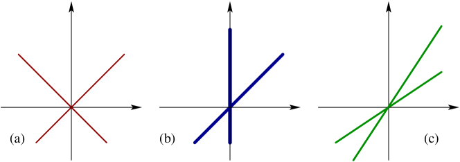
Figure 1: Comparison of the light-cone coordinates $u,\bar{u}$ for (a) $2D$ ortho-conformal transformations, (b) $1D$ meta-conformal transformations with $\alpha=0$ and (c) $1D$ meta-conformal transformations with $\alpha\neq 0$.

Summarising, we have have found the distinct kinds of time-space transformations which arise from the conformal algebra in $(1+1)D$, under the assumption stated above.

Proposition 1: For $1+1$ time-space dimensions, the distinct representations as time-space transformations of the conformal algebra (1.2) are listed in table 2. The choice of orthogonal coordinates $u,\bar{u}$ corresponds to ortho-conformal transformations, while meta-conformal transformations are found if non-orthogonal coordinates $u,\bar{u}$ are used.

The different physical interpretations of the light-cone coordinates $u,\bar{u}$ are illustrated in figure 1. Clearly, the ‘natural’ coordinates of $1D$ meta-conformal transformations do not correspond to orthogonal coordinates, while ortho-conformal transformations are obtained for orthogonal coordinates.

2.2 Finite $1D$ meta-conformal transformations

A more clear geometric picture of the meta-conformal transformations of table 2 can be found by constructing the Lie series $F_{Y}(\varepsilon,t,r)=e^{\varepsilon Y_{m}}F(0,t,r)$ and $F_{X}(\varepsilon,t,r)=e^{\varepsilon X_{n}}F(0,t,r)$ of the corresponding finite transformations. If we use the representation (1.8), they are given as the solutions of the two initial-value problems (herein, $\alpha=0$)

$$\Bigl{(}\partial_{\varepsilon}+(t+\mu r)^{m+1}\partial_{r}+(m+1)\gamma(t+\mu r)^{m}\Bigr{)}F_{Y}(\varepsilon,t,r)=0$$ (2.16a)

$$\Bigl{(}\partial_{\varepsilon}+t^{n+1}\partial_{t}+\mu^{-1}\left[(t+\mu r)^{n+1}-t^{n+1}\right]\partial_{r}+(n+1)\left(\delta t^{n}+\frac{\gamma}{\mu}\left[(t+\mu r)^{n}-t^{n}\right]\right)\Bigr{)}F_{X}(\varepsilon,t,r)=0$$ (2.16b)

subject to the initial conditions $F_{X}(0,t,r)=F_{Y}(0,t,r)=\varphi(t,r)$. If we work with the variable $\rho=t+\mu r$ instead of $r$, we write the initial condition $F_{X}(0,t,\rho)=F_{Y}(0,t,\rho)=\phi(t,\rho):=\varphi(t,r)$ and find, with the conformal weights $\Delta$, $\overline{\Delta}$ taken from table 2

$$Y_{m}: \quad\phi^{\prime}(t,\rho)=\left(\frac{{\rm d}\rho^{\prime}}{{\rm d}\rho}\right)^{\overline{\Delta}}\phi(t^{\prime},\rho^{\prime})\;\;\hskip 46.94687pt;\;\;t^{\prime}=t\;\;,\;\;\rho^{\prime}=a(\rho)$$ (2.17a)

$$X_{n}: \quad\phi^{\prime}(t,\rho)=\left(\frac{{\rm d}t^{\prime}}{{\rm d}t}\right)^{\Delta}\left(\frac{{\rm d}\rho^{\prime}}{{\rm d}\rho}\right)^{\overline{\Delta}}\phi\left(t^{\prime},\rho^{\prime}\right)\;\;;\;\;t^{\prime}=b(t)\;\;,\;\;\rho^{\prime}=b(\rho)$$ (2.17b)

where $a=a(\rho)$ and $b=b(t)$ are arbitrary differentiable functions. The transformation of $r$ as generated by $X_{n}$ reads

$$r^{\prime}=\frac{1}{\mu}[b(t+\mu r)-b(t)].$$ (2.18)

Re-expanding $b(t)=t-\varepsilon t^{n+1}$ and $a(\rho)=\rho-\varepsilon\rho^{m+1}$ reproduces the differential equations (2.16) for the Lie series. Alternatively, if $\alpha\neq 0$, we can use the representation (2.13), and work with the variables $u$ and $\bar{u}$, as well as with the conformal weights $\Delta$ and $\overline{\Delta}$, as given in table 2 and find

$${\cal Y}_{m}: \quad\phi^{\prime}(u,\bar{u})=\left(\frac{{\rm d}\bar{u}^{\prime}}{{\rm d}\bar{u}}\right)^{\overline{\Delta}}\phi(u^{\prime},\bar{u})\;\;\hskip 7.11317pt;\;\;u^{\prime}=u\;\;,\;\;\bar{u}^{\prime}=\bar{f}(\bar{u})$$ (2.19a)

$$A_{n}: \quad\phi^{\prime}(u,\bar{u})=\left(\frac{{\rm d}u^{\prime}}{{\rm d}u}\right)^{\Delta}\phi\left(u^{\prime},\bar{u}^{\prime}\right)\;\;;\;\;u^{\prime}=f(u)\;\;,\;\;\bar{u}^{\prime}=\bar{u}$$ (2.19b)

and where $f=f(u)$ and $\bar{f}=\bar{f}(\bar{u})$ are arbitrary differentiable functions. This is the statement already contained in table 1, which remains valid for $\alpha=0$ and $\alpha\neq 0$.

Eqs. (2.17,2.19) give the global form of the $1D$ meta-conformal transformations and show how a primary meta-conformal scaling operator should be defined, generalising the concept from the case of orthogonal coordinates studied in [11] to non-orthogonal coordinates. In this work, we shall concentrate on finding new meta-conformal transformations and we shall leave the construction of the full conformal field-theory based on (2.17,2.19) to future work.

2.3 Ansatz for the $d$-dimensional case

Meta-conformal transformations are analogues of the conformal algebra $\mathfrak{conf}(d)$ and are sought as dynamical symmetries of a ballistic transport equation, with a constant $\bm{c}\in\mathbb{R}^{d}$,

$$\hat{\mathscr{S}}\phi(t,\bm{r})=(\partial_{t}+\bm{c}\cdot\bm{\partial}_{\bm{r}})\phi(t,\bm{r})=0$$ (2.20)

This naturally generalises eq. (1.11). Our construction starts from two axioms:

(i) The generators of translations and time-space dilatations read in $d$ dimensions

$$X_{-1} =-\partial_{t}$$ (2.21a)

$$Y^{j}_{-1} =-\partial_{r_{j}}\;\;,\quad j\in\{1,\ldots,d\}$$ (2.21b)

$$X_{0} =-t\partial_{t}-\bm{r}\cdot\partial_{\bm{r}}-\delta$$ (2.21c)

where $\delta$ stands for a scaling dimension. If $d\leq 3$, we shall also write $j\in\{x,y,z\}$.

(ii) Specifying $X_{1}$ fixes all further generators. We make the ansatz

$$X_{1} := -(t^{2}+\alpha\bm{r}^{2})\partial_{t}-2t\bm{r}\cdot\partial_{\bm{r}}-p(\bm{r}\cdot\bm{r})\bm{\beta}\cdot\partial_{\bm{r}}-(1-p)(\bm{\beta}\cdot\bm{r})\bm{r}\cdot\partial_{\bm{r}}-2\delta t$$ (2.22)

$$-\bm{B}(\bm{r},\bm{\beta},\bm{\gamma})\cdot\partial_{\bm{\gamma}}-k\bm{\gamma}\cdot\bm{r}$$

where $\alpha$, $p$ and $k$ are scalars, $\bm{\beta}$, $\bm{\gamma}$ are vectors and the vector $\bm{B}$ depends on its arguments. All these must be found self-consistently from the algebra we are going to construct.

By construction, $[X_{n},X_{m}]=(n-m)X_{n+m}$ is obeyed for $n,m\in\{\pm 1,0\}$. All further generators of the Lie algebra will be obtained from repeated commutators of $X_{1}$ with $X_{-1}$ and $Y_{-1}^{j}$, using $\left[X_{1},Y_{m}^{j}\right]=(1-m)Y_{m+1}^{j}$. The form (2.22) of the generator $X_{1}$ is motivated as follows.

• For $d=1$ dimension, one should reproduce $X_{1}$ in eq. (2.1). The $1D$ generator contains a term $-\beta r^{2}\partial_{r}$, which for $d>1$ leads to two distinct contributions, as specified in (2.22).

• $X_{1}$ should be rotation-invariant, that is it should commute with the generators $R_{ij}$ of spatial rotations. However, for the ‘natural’ choice $R_{ij}=r_{i}\partial_{r_{j}}-r_{j}\partial_{r_{i}}$, the invariance condition $\left[X_{1},R_{ij}\right]=0$ does not hold, not even in the special case $\bm{B}=\bm{\gamma}=0$. Therefore, spatial rotations should also include rotations of the vectors $\bm{\beta}$ and $\bm{\gamma}$. The rotation generator becomes

  $$\bar{R}_{ij}=\left(r_{i}\partial_{r_{j}}-r_{j}\partial_{r_{i}}\right)+\varepsilon_{\gamma}\left(\gamma_{i}\partial_{\gamma_{j}}-\gamma_{j}\partial_{\gamma_{i}}\right)+\varepsilon_{\beta}\left(\beta_{i}\partial_{\beta_{j}}-\beta_{j}\partial_{\beta_{i}}\right)$$ (2.23)

  where the signatures $\varepsilon_{\gamma},\varepsilon_{\beta}=\pm 1$ allow for a different sense of rotation of $\bm{\beta}$ or $\bm{\gamma}$ than of the spatial coordinates $\bm{r}$. Furthermore, we should allow for the possibility $\bm{B}\neq\bm{0}$. In addition, from the commutation relation of the one-dimensional case (1.9), especially $[[X_{1},Y^{j}_{-1}],Y_{-1}^{j}]\sim Y_{-1}^{j}$, and (2.21b), it follows that $\bm{B}$ can be at most linear in $\bm{r}$.

Additional restrictions on the form of $X_{1}$ come from the requirement that it should act as a dynamical symmetry of eq. (2.20). By ‘dynamical symmetry’ we mean the following required commutator [77]

$$[\hat{\mathscr{S}},X_{1}]\phi=\lambda(t,\bm{r})\hat{\mathscr{S}}\phi.$$ (2.24)

which implies that the space of solutions of $\hat{\mathscr{S}}\phi=0$ is invariant under the action of $X_{1}$ (eventually after fixing one or several scaling dimensions of $\phi$ to certain values). As we shall see, this requirement leads to new relations between $\alpha,p$ and $\bm{\beta}$.

Example: The two vectors $\bm{\beta}$ and $\bm{c}$ span a two-dimensional space. By rotation-invariance, it is therefore enough to consider the case $d=2$, since any higher-dimensional situation can be reduced to the present case. Let $\bm{B}=\bm{\gamma}=\bm{0}$. From (2.22,2.24) it follows that $\delta=0$ and

$$1+\beta_{x}c_{x}+\frac{1-p}{2}\beta_{y}c_{y} =\alpha c_{x}^{2}$$ (2.25a)

$$p\beta_{x}c_{y}+\frac{1-p}{2}\beta_{y}c_{x} =\alpha c_{x}c_{y}$$ (2.25b)

$$1+\frac{1-p}{2}\beta_{x}c_{x}+\beta_{y}c_{y} =\alpha c_{y}^{2}$$ (2.25c)

$$p\beta_{y}c_{x}+\frac{1-p}{2}\beta_{x}c_{y} =\alpha c_{x}c_{y}$$ (2.25d)

We look for a solution of the above system for $\bm{\beta}\neq\bm{0}$. Straightforward calculations show:

1. The case $p=1$ leads to contradictions between some of the equations in the system (2.25). Then the generator $X_{1}$ cannot be a symmetry.

2. For $p\neq 1$, we have the following solution of the system (2.25)

   $$c_{j} =\frac{2}{p-1}\frac{\beta_{j}}{\bm{\beta}^{2}}\;\;,\quad j=x,y$$ (2.26a)

   $$\alpha =\frac{1}{4}(p+1)(p-1)\>\bm{\beta}^{2}$$ (2.26b)

   Hence, the condition (2.24) is satisfied, with $\lambda(t,\bm{r})=-2t-(p+1)(\bm{\beta}\cdot\bm{r})$. In contrast with the $1D$ case, $\alpha$ is fixed by (2.26b) in terms of $\bm{\beta}$. In particular, $\alpha=0$ is only possible for $p=-1$. The solution (2.26) holds true for all dimensions $d>1$.

   Eq. (2.26a) shows that $\bm{c}$ and $\bm{\beta}$ are collinear. Calculations are simplified by choosing the orientation of the coordinate axes such that only $\beta_{1}=\beta_{x}\neq 0$ and $\beta_{j}=0$ for all $j\geq 2$.

3. For $d=1$, only eq. (2.25a) remains, which is equivalent to (2.4). Hence the structure of the $1D$ meta-conformal algebra is distinct from the one in any other dimension $d>1$.

In general, $\bm{B}\neq\bm{0}$ depends linearly on $\bm{r}$. Then the sought symmetries generated by $X_{1}$ can become conditional symmetries, that is some auxiliary conditions on the field $\varphi=\varphi(t,\bm{r},\bm{\beta},\bm{\gamma})$ must be imposed, see [13, 38, 39, 25] and references therein. We shall come back to this at the end of section 3.

3 Meta-conformal algebra in $d>1$ spatial dimensions

We now find the Lie algebra $\mathfrak{meta}(1,d)$ in more than one spatial dimension $d$. We begin with generic conditions which will hold for any dimension $d>1$. Specific results apply for $d=2$ and will be presented in section 4.

We start from the ansatz (2.22), with $p\neq 1$. Throughout, we shall assume $\bm{B}=\bm{0}$, unless explicitly stated otherwise. From the defining commutator relation, we have the generator

$$Y_{0}^{j} := \frac{1}{2}[X_{1},Y_{-1}^{j}]$$ (3.1)

$$= -\alpha r_{j}\partial_{t}-\left(t+\frac{1}{2}(1-p)(\bm{\beta}\cdot\bm{r})\right)\partial_{r_{j}}-pr_{j}\bm{\beta}\cdot\partial_{\bm{r}}-\frac{1}{2}(1-p)\beta_{j}\bm{r}\cdot\partial_{\bm{r}}-(k/2)\gamma_{j}~{}~{}~{}~{}$$

To be specific, let $d=3$, but the conclusions will apply to any $d\geq 2$. Take from (2.26b) the value $\alpha=\frac{1}{4}(p-1)(p+1)\bm{\beta}^{2}$ and work out $[Y_{0}^{j},Y_{0}^{i}]$ for $i\neq j$. For example

$$[Y_{0}^{x},Y_{0}^{y}] = \frac{(3p-1)(p+1)(p-1)}{8}(\beta_{y}x-\beta_{x}y)\partial_{t}$$ (3.2)

$$+\left(\frac{(3p-1)(p+1)}{4}(\beta_{x}\beta_{y}x-\beta_{x}^{2}y)+\frac{(1-p)^{2}}{4}(\beta_{z}^{2}y-\beta_{y}\beta_{z}z)\right)\partial_{x}$$

$$+\left(\frac{(3p-1)(p+1)}{4}(\beta_{y}^{2}x-\beta_{x}\beta_{y}y)-\frac{(1-p)^{2}}{4}(\beta_{z}^{2}x-\beta_{x}\beta_{z}z)\right)\partial_{y}$$

$$+p^{2}(\beta_{y}\beta_{z}x-\beta_{x}\beta_{z}y)\partial_{z}$$

which must be expressed in terms of the generators of the Lie algebra under construction, including the rotation generators $R_{ij}=r_{i}\partial_{r_{j}}-r_{j}\partial_{r_{i}}$. From (3.2) we see that the commutator $[Y_{0}^{x},Y_{0}^{y}]$ only becomes a linear combination of known generators if the parameter $p$ obeys

$$p^{2}-\frac{1}{4}(1-p)^{2}=\frac{1}{4}(p+1)(3p-1)\stackrel{{\scriptstyle!}}{{=}}0,$$ (3.3)

Proposition 2: Consistent representations of $\mathfrak{meta}(1,d)$ with $d>1$ are only possible in the cases (i) $p_{1}=-1$ and (ii) $p_{2}=\frac{1}{3}$.

In either of these cases, the commutator (3.2) simplifies to

$$[Y_{0}^{x},Y_{0}^{y}] =-p^{2}\left(\beta_{z}^{2}R_{xy}+\beta_{x}\beta_{z}R_{yz}+\beta_{y}\beta_{z}R_{zx}\right)$$ (3.4a)

Similarly, for the same values of $$p=-1,\frac{1}{3} d=3$$, we find (still for )

$$[Y_{0}^{y},Y_{0}^{z}]=-p^{2}\left(\beta_{x}\beta_{z}R_{xy}+\beta_{x}^{2}R_{yz}+\beta_{x}\beta_{y}R_{zx}\right)$$ (3.4b)

$$[Y_{0}^{z},Y_{0}^{x}]=-p^{2}\left(\beta_{y}\beta_{z}R_{xy}+\beta_{x}\beta_{y}R_{yz}+\beta_{y}^{2}R_{zx}\right)$$ (3.4c)

Therefore, a discussion of rotation-invariance is necessary.

1. One might choose to keep full spatial rotation-invariance, with all three generators $R_{xy}$, $R_{yz}$, $R_{zx}$. Since the invariant equation (2.20) contains a vector proportional to $\bm{\beta}$, one must include into the rotation generators, viz. $R_{ij}\mapsto\bar{R}_{ij}$, terms which describe the simultaneous rotations of the position $\bm{r}$ and of $\bm{\beta}$. However, changing $\bm{\beta}$ then implies changing the invariant equation. The transformations found will map one equation of the type (2.20) to another equation of the same type.

2. Here, we shall use rotation-invariance to orient the coordinate axes such that $\bm{\beta}$ is along the $x$-axis. In other words, we shall fix, from now on, $\beta_{x}=\beta\neq 0$ and $\beta_{y}=\beta_{z}=\ldots=0$. Explicit rotation-invariance will only apply to rotations which leave the $x$-axis invariant. These do not exist for $d=2$, but for $d=3$ we have the rotation $R=R_{yz}$.

3.1 Meta-conformal algebra in $d=3$ dimensions with $\bm{\gamma}=\bm{0}$

The case of $d=3$ spatial dimensions gives the generic structure meta-conformal transformations. Throughout, we shall fix $\bm{\beta}=(\beta,0,0)$. First, we restrict to the more simple case $\bm{\gamma}=\bm{0}$. The rotation generator is $R_{ij}=r_{i}\partial_{r_{j}}-r_{j}\partial_{r_{i}}$. With (2.26b), we have

$$X_{1} = -\left(t^{2}+\alpha(x^{2}+y^{2}+z^{2})\right)\partial_{t}-\left(2tx+\beta x^{2}+\beta p(y^{2}+z^{2})\right)\partial_{x}$$ (3.5)

$$-(2t+\frac{1-p}{2}\beta x)y\partial_{y}-(2t+\frac{1-p}{2}\beta x)z\partial_{z}-2\delta t.$$

All other generators can be found from (3.5). Starting from $Y_{0}^{j}:=\frac{1}{2}[X_{1},Y_{-1}^{j}]$, we check that $[Y_{0}^{x},Y_{0}^{y}]=[Y_{0}^{x},Y_{0}^{z}]=0$. In addition, if we take either $p=-1$ or $p=\frac{1}{3}$, then

$$[Y_{0}^{y},Y_{0}^{z}]=-p^{2}\beta^{2}R_{yz}$$ (3.6)

does not vanish for $d\geq 3$, see (3.4b). Also, $[X_{1},R_{yz}]=0$, as expected from rotation-invariance. The next family of generators is obtained from $Y_{1}^{j}:=[X_{1},Y_{0}^{j}]$. If $n,m\in\{-1,0,1\}$ and $j=x,y,z$, the non-vanishing commutators are compactly written as

$$[X_{n},X_{m}]=(n-m)X_{n+m}\;\;,\quad[X_{n},Y_{m}^{j}]=(n-m)Y_{n+m}^{j}$$

$$[Y_{n}^{x},Y_{m}^{x}]=(n-m)(\alpha X_{n+m}+\beta Y_{n+m}^{x})$$

$$[Y_{n}^{y},Y_{m}^{y}]=[Y_{n}^{z},Y_{m}^{z}]=(n-m)(\alpha X_{n+m}+p\beta Y_{n+m}^{x})$$

$$[Y_{n}^{x},Y_{m}^{w}]=[Y_{n}^{w},Y_{m}^{x}]=(n-m)\frac{1-p}{2}\beta Y_{n+m}^{w}~{}~{}\mbox{\rm;~{}~{} for $w=y,z$,}$$

$$[Y_{n}^{y},Y_{m}^{z}]=\delta_{n+m,0}(n-m-\delta_{nm})p^{2}\beta^{2}R_{yz},$$ (3.7)

$$[Y_{m}^{y},R_{yz}]=Y_{m}^{z}\;\;,\quad[Y_{m}^{z},R_{yz}]=-Y_{m}^{y}.$$

Proposition 3: If $p=-1$ or $p=\frac{1}{3}$, and $\bm{\gamma}=\bm{0}$, the set $\mathfrak{meta}(1,3):=\langle X_{0,\pm 1},Y_{0,\pm 1}^{x,y,z},R_{yz}\rangle$ of differential operators, as derived from (3.5), closes into a meta-conformal Lie algebra, whose structure is determined by the commutators (3.7), with two distinct representations.

Proof: The first part of the proposition follows from the closure of the commutators (3.7). For the second part, let $p=\frac{1}{3}$ and consider the commutators (3.7). Re-define the generators $Y_{n}^{x}\mapsto{\cal Y}_{n}^{x}:=-\frac{2}{3}\beta X_{n}+Y_{n}^{x}$. Again, the commutators (3.7) will hold, where $Y_{n}^{x}$ is substituted by ${\cal Y}_{n}^{x}$ and if one replaces therein $\beta\mapsto-(\beta/3)$. q.e.d.

For clarity, we shall mainly concentrate on the most simple representation, with $p=-1$. For easy reference, we repeat below the commutators of the $p=-1$ representation of $\mathfrak{meta}(1,3)$ (here $n,m\in\{-1,0,1\}$ and $j=x,y,z$)

$$[X_{n},X_{m}]=(n-m)X_{n+m}\;\;,\quad[X_{n},Y_{m}^{j}]=(n-m)Y_{n+m}^{j}$$

$$[Y_{n}^{x},Y_{m}^{x}]=(n-m)\beta Y_{n+m}^{x}$$

$$[Y_{n}^{y},Y_{m}^{y}]=[Y_{n}^{z},Y_{m}^{z}]=-(n-m)\beta Y_{n+m}^{x}$$

$$[Y_{n}^{x},Y_{m}^{w}]=[Y_{n}^{w},Y_{m}^{x}]=(n-m)\beta Y_{n+m}^{w}~{}~{}\mbox{\rm;~{}~{} for $w=y,z$,}$$

$$[Y_{n}^{y},Y_{m}^{z}]=\delta_{n+m,0}(n-m-\delta_{nm})\beta^{2}R_{yz},$$ (3.8)

$$[Y_{m}^{y},R_{yz}]=Y_{m}^{z}\;\;,\quad[Y_{m}^{z},R_{yz}]=-Y_{m}^{y}.$$

The structure of meta-conformal algebras can be further simplified. This is in contrast with the semi-direct sums which hold true e.g. for the Schrödinger algebra.

Proposition 4: The Lie algebra $\mathfrak{meta}(1,3)$ decomposes as a direct sum

$$\mathfrak{meta}(1,3)\cong\mathfrak{sl}(2,\mathbb{R})\oplus\mathfrak{conf}(3)\cong\mathfrak{sl}(2,\mathbb{R})\oplus B_{2}.$$ (3.9)

Proof: The relations (3.8) imply that $\langle X_{0,\pm 1}\rangle\cong\mathfrak{sl}(2,\mathbb{R})$. In addition, the action of the $\mathfrak{sl}(2,\mathbb{R})$-subalgebra on the generators of the subalgebra $\mathfrak{g}:=\langle Y_{m}^{x,y,z},R\rangle_{m\in\{\pm 1,0\}}$, with $R=R_{yz}$ shows a semi-direct structure. Changing the base of the Lie algebra according to $X_{n}\mapsto A_{n}:=X_{n}-Y_{n}^{x}/\beta$, one has $\langle A_{\pm 1,0}\rangle\cong\mathfrak{sl}(2,\mathbb{R})$ and the direct sum $\mathfrak{meta}(1,3)\cong\mathfrak{sl}(2,\mathbb{R})\oplus\mathfrak{g}$, as can be checked through the commutators

$$[A_{n},Y_{m}^{x}]=[A_{n},Y_{m}^{y}]=[A_{n},Y_{m}^{z}]=[A_{n},R]=0.$$

The structure of the Lie sub-algebra $\mathfrak{g}$ is made clear by defining the generators

$$Y_{n}^{+}=Y_{n}^{y}+{\rm i}Y_{n}^{z}\;\;,\;\;Y_{n}^{-}=Y_{n}^{y}-{\rm i}Y_{n}^{z}.$$

Then the non-vanishing commutators of the Lie algebra $\mathfrak{g}$ become

$$[Y_{n}^{x},Y_{m}^{x}]=(n-m)\beta Y_{n+m}^{x}\;\;,\;\;[Y_{n}^{x},Y_{m}^{\pm}]=(n-m)\beta Y_{n+m}^{\pm}\;\;,\;\;[R,Y_{m}^{\pm}]=\pm{\rm i}Y_{m}^{\pm}$$

$$[Y_{n}^{+},Y_{m}^{-}]=\left\{\begin{array}[]{lll}2(n-m)\beta Y_{n+m}^{x}&\mbox{\rm~{}~{};~{} if $n+m\neq 0$}\\ 2{\rm i}\beta^{2}R&\mbox{\rm~{}~{};~{} if $n=m=0$}\\ 2(n-m)\beta Y_{n+m}^{x}-4{\rm i}\beta^{2}R&\mbox{\rm~{}~{};~{} if $n\neq m$}\end{array}\right.$$

The correspondence with the roots of the complex Lie algebra $B_{2}$ is shown in figure 2. q.e.d.

Figure 2: Root diagramme of the complex Lie algebra $B_{2}$ and the correspondence with generators of $3D$ meta-conformal transformations.

Although we did not carry out the explicit construction of the generators for $d>3$ dimensions, counting their number allows to formulate the following

Conjecture: In $d\geq 1$ spatial dimensions, one has for $\mathfrak{meta}(1,d)$ the Lie algebra isomorphisms

$$\mathfrak{meta}(1,1)\cong A_{1}\oplus A_{1}\;\;,\;\;\mathfrak{meta}(1,d)\cong\mathfrak{sl}(2,\mathbb{R})\oplus\mathfrak{conf}(d)\cong\left\{\begin{array}[]{ll}A_{1}\oplus D_{n+1}&\mbox{\rm~{}~{};~{} if $d=2n$}\\ A_{1}\oplus B_{n+1}&\mbox{\rm~{}~{};~{} if $d=2n+1$}\end{array}\right.$$ (3.10)

with $n=1,2,\ldots$, and where $\mathfrak{conf}(d)$ is the ortho-conformal Lie algebra in $d$ dimensions and $A_{1}$, $B_{n}$, $D_{n}$ are simple complex Lie algebras from Cartan’s classification (and $D_{2}\cong A_{1}\oplus A_{1}$).

In stating this, we anticipate results on $\mathfrak{meta}(1,2)$ from sect. 4.

A further important difference between $d=2$ and $d\geq 3$ dimensions arises from the non-vanishing of commutators such as (3.6) when $d\geq 3$. The vanishing of these commutators for $d=2$ is the reason why an infinite-dimensional extension of the $2D$ meta-conformal Lie algebra can be constructed, as we shall show in section 4.

3.2 Meta-conformal algebra in $d=3$ dimensions with $\bm{\gamma}\neq\bm{0}$

We first redefine the generator of rotations, which now should include rotations of $\bm{\gamma}$

$$R_{yz}\mapsto\bar{R}_{yz}=:y\partial_{z}-z\partial_{y}+\gamma_{y}\partial_{\gamma_{z}}-\gamma_{z}\partial_{\gamma_{z}}.$$ (3.11)

Here, we must also include the term $\bm{B}\neq\bm{0}$. To do so, we modify $X_{1}$ of eq. (3.5) by the following ansatz, according to (2.22)

$$X_{1} \mapsto X_{1}+\tilde{X}_{1}$$

$$\tilde{X}_{1} = -\left(a(\bm{\beta}\cdot\bm{r})\bm{\gamma}+b(\bm{\gamma}\cdot\bm{r})\bm{\beta}+c(\bm{\beta}\cdot\bm{\gamma})\bm{r}\right)\cdot\partial_{\bm{\gamma}}-k(\bm{\gamma}\cdot\bm{r})$$ (3.12)

$$= -\beta\left((a+b+c)x\gamma_{x}+a(y\gamma_{y}+z\gamma_{z})\right)\partial_{\gamma_{x}}-k(x\gamma_{x}+y\gamma_{y}+z\gamma_{z})$$

$$-\beta(bx\gamma_{y}+cy\gamma_{x})\partial_{\gamma_{y}}-\beta(bx\gamma_{z}+cz\gamma_{x})\partial_{\gamma_{z}}$$

where $a,b,c$ and $k$ are constants to be determined. Next, we construct $Y_{0}^{x,y,z}$ and $Y_{1}^{x,y,z}$, as usual.${}^{\ref{ftn:calc}}$ We find the explicit extra terms beyond (3.1)

$$Y_{0}^{x}\mapsto Y_{0}^{x}+\tilde{Y}_{0}^{x},\quad Y_{0}^{y}\mapsto Y_{0}^{y}+\tilde{Y}_{0}^{y},\quad Y_{0}^{z}\mapsto Y_{0}^{z}+\tilde{Y}_{0}^{z}$$

$$\tilde{Y}_{0}^{x}=-(\beta/2)\left((a+b+c)\gamma_{x}\partial_{\gamma_{x}}+b(\gamma_{y}\partial_{\gamma_{y}}+\gamma_{z}\partial_{\gamma_{z}}\right)-(k/2)\gamma_{x}$$ (3.13a)

$$\tilde{Y}_{0}^{y}=-(\beta/2)(a\gamma_{y}\partial_{\gamma_{x}}+c\gamma_{x}\partial_{\gamma_{y}})-(k/2)\gamma_{y}$$ (3.13b)

$$\tilde{Y}_{0}^{z}=-(\beta/2)(a\gamma_{z}\partial_{\gamma_{x}}+c\gamma_{x}\partial_{\gamma_{z}})-(k/2)\gamma_{z}$$ (3.13c)

The values of the constants $a,b,c$ are fixed from the requirement that the Lie algebra commutators of $\mathfrak{meta}(1,3)$ are those of the case $\bm{\gamma}=\bm{0}$ treated above. Eqs. (3.13) imply

1. the conditions $[Y_{0}^{x},Y_{0}^{y}]=[\tilde{Y}_{0}^{x},\tilde{Y}_{0}^{y}]=0$ yield $a=b=-c$.

2. the condition $[Y_{0}^{y},Y_{0}^{z}]=-p^{2}\beta^{2}\bar{R}_{yz}$ yields $a=\pm 2p$.

Proposition 5: The time-space $3D$ meta-conformal transformations with $\bm{\gamma}\neq\bm{0}$ can be labelled by the pair $(p,a)$. There are four possibilities: $(p,a)=(-1,-2)$, $(-1,2)$, $(\frac{1}{3},\frac{2}{3})$, $(\frac{1}{3},-\frac{2}{3})$. The value of the constant $k$ is not fixed by the commutators.

The commutator $Y_{1}^{j}=[X_{1},Y_{0}^{j}]$ gives the corresponding extensions of the generators $Y_{1}^{j}$.

3.3 Symmetries of the ballistic transport equation

Returning to the linear ballistic transport equation, in the form (2.20,2.26a)

$$\hat{\mathscr{S}}\varphi_{\bm{\gamma}}(t,\bm{r})=\left(\partial_{t}+\frac{2}{\beta(p-1)}\partial_{x}\right)\varphi_{\bm{\gamma}}(t,\bm{r})=0.$$ (3.14)

we can state the conditions for it having a meta-conformal dynamical symmetry, for $\bm{\gamma}\neq\bm{0}$ and $\bm{B}\neq\bm{0}$. Herein, the solution $\varphi=\varphi_{\bm{\gamma}}(t,\bm{r})$ may also depend on the vector $\bm{\gamma}$ of ‘rapidities’.

Proposition 6: For generic dimension $d>2$, and $p=\frac{1}{3}$ or $p=-1$, we have

• For $\bm{\gamma}=\bm{0}$, the meta-conformal representations constructed above leave invariant the solution space of the equations (3.14), under the condition $\delta=0$.

• For $\bm{\gamma}\neq\bm{0}$ and if $\varphi_{\bm{\gamma}}(t,\bm{r})=\varphi(t,\bm{r})$ does not explicitly depend on $\bm{\gamma}$, the corresponding meta-conformal representation leaves the solution space of (3.14) invariant, if $k=1$ and $\gamma_{x}=(1-p)\beta\delta$.

• If the solution $\varphi_{\bm{\gamma}}(t,\bm{r})$ does also depend on $\bm{\gamma}$, invariance of the solution space of (3.14) is only obtained under the conditions $k=1$ and

  $$\left(\delta+\frac{1}{\beta(p-1)}\gamma_{x}+\frac{a}{p-1}\bm{\gamma}\cdot\partial_{\bm{\gamma}}\right)\varphi_{\bm{\gamma}}(t,\bm{r})=0$$ (3.15)

In case (iii) we have an on-shell or a conditional symmetry of eq. (3.14), see e.g. [13, 39, 25].

Proof: This follows from the non-vanishing commutators

$$\left[\hat{\mathscr{S}},X_{0}\right] = -\hat{\mathscr{S}}\;\;,\hskip 71.13188pt\;\;\left[\hat{\mathscr{S}},Y_{0}^{x}\right]=-\frac{p+1}{2}\beta\hat{\mathscr{S}}$$

$$\left[\hat{\mathscr{S}},X_{1}\right] = -\left(2t+(p+1)\beta x\right)\hat{\mathscr{S}}-2\left(\delta+\frac{k}{\beta(p-1)}\gamma_{x}+\frac{a}{p-1}\bm{\gamma}\cdot\partial_{\bm{\gamma}}\right)$$

$$\left[\hat{\mathscr{S}},Y_{1}^{x}\right] = -\frac{\beta(p+1)}{2}\left(2t+(p+1)\beta x\right)\hat{\mathscr{S}}$$

$$-(p+1)\beta\left(\delta+\frac{2+(p-1)k}{(p-1)(p+1)\beta}\gamma_{x}+\frac{a}{p-1}\bm{\gamma}\cdot\partial_{\bm{\gamma}}\right)$$

and recalling that $a=\pm 2p$. q.e.d.

4 Meta-conformal algebra in $d=2$ spatial dimensions

Finding meta-conformal transformations in $d=2$ space dimensions (with points $(t,x,y)\in\mathbb{R}^{3}$) proceeds as follows. As in sections 2 and 3, the generators of translations and dilatations read

$$X_{-1} =-\partial_{t}$$ (4.1a)

$$Y^{x}_{-1} =-\partial_{x}\;\;,\;\;Y^{y}_{-1}=-\partial_{y}$$ (4.1b)

$$X_{0} =-t\partial_{t}-x\partial_{x}-y\partial_{y}-\delta.$$ (4.1c)

The form of $X_{1}$ is given by (2.22) where for simplicity we set $\bm{B}=\bm{0}$ and fixed $k=2$. Explicitly

$$X_{1} = -\left(t^{2}+\alpha(x^{2}+y^{2})\right)\partial_{t}-\left(2tx+\beta_{x}x^{2}+(1-p)\beta_{y}xy+p\beta_{x}y^{2}\right)\partial_{x}$$ (4.2)

$$-\left(2ty+p\beta_{y}x^{2}+(1-p)\beta_{x}xy+\beta_{y}y^{2}\right)\partial_{y}-2\delta t-2\gamma_{x}x-2\gamma_{y}y.$$

and we kept the vector $\bm{\beta}=(\beta_{x},\beta_{y})$ arbitrary. In complete analogy with the case of $d\geq 3$ dimensions, the generators of the nine-dimensional Lie algebra $\mathfrak{meta}(1,2)=\left\langle X_{n},Y_{n}^{j}\right\rangle_{n\in\{\pm 1,0\},j\in\{x,y\}}$ are found,${}^{\ref{ftn:calc}}$ for the two admissible cases (i) $p=-1$ and (ii) $p=\frac{1}{3}$. However, the Lie algebra of $2D$ meta-conformal transformations is infinite-dimensional, as we shall now show.

4.1 Infinite-dimensional extension

transformation		$\tau$	$w$	$\bar{w}$
meta-conformal $2D$ i	$\alpha=0$	$t$	$t+\beta(x+{\rm i}y)$	$t+\beta(x-{\rm i}y)$
meta-conformal $2D$ ii	$\alpha\neq 0$	$t+\frac{2\beta}{3}\,x$	$t+\frac{\beta}{3}\,(x-{\rm i}y)$	$t+\frac{\beta}{3}\,(x+{\rm i}y)$

Table 3: Possible choices for the ‘time’ and ‘complex’ light-cone coordinates $\tau,w,\bar{w}$ of the $2D$ meta-conformal generators (4.3) in $d=2$ spatial dimensions, in terms of the time-space coordinates $t,x,y$.

In what follows, we shall choose coordinate axes such that $\bm{\beta}=(\beta,0)$.

Proposition 7: Consider the set of generators, with $n\in\mathbb{Z}$

$$A_{n} = -\tau^{n+1}\partial_{\tau}-(n+1)\vartheta\,\tau^{n}$$

$$B_{n}^{+} = -w^{n+1}\partial_{w}-(n+1)\Delta\,w^{n}$$ (4.3)

$$B_{n}^{-} = -\bar{w}^{n+1}\partial_{\bar{w}}-(n+1)\overline{\Delta}\,\bar{w}^{n}$$

which act on the time-space coordinates $(\tau,w,\bar{w})$. Their non-vanishing commutators are

$$\left[A_{n},A_{m}\right]=(n-m)A_{n+m}\;\;,\;\;\left[B_{n}^{\pm},B_{m}^{\pm}\right]=(n-m)B_{n+m}^{\pm}$$ (4.4)

The two possible cases of $2D$ meta-conformal transformations correspond to (i) $p=-1$ with $\alpha=0$ and (ii) $p=\frac{1}{3}$ with $\alpha=-\frac{2}{9}\bm{\beta}^{2}\neq 0$. The relationship with the usual time-space coordinates $(t,x,y)$ is given, for both cases, in table 3 and the meta-conformal weights are in table 4.

Proof: straightforward calculation. The correspondence with the representations of the finite-dimensional sub-algebra $\mathfrak{meta}(1,2)$ will be given in eqs. (4.9,4.17) below. q.e.d.

The Lie algebra (4.4) is isomorphic to the direct sum $\mathfrak{vect}(S^{1})\oplus\mathfrak{vect}(S^{1})\oplus\mathfrak{vect}(S^{1})$, the direct sum of three centre-less Virasoro algebras. The corresponding meta-conformal weights $\vartheta$, $\Delta$, $\overline{\Delta}$ are expressed in table 4 in terms of the scaling dimension $\delta$ and the two ‘rapidities’ $\gamma_{x,y}$.

transformation		$\vartheta$	$\Delta$	$\overline{\Delta}$
meta-conformal $2D$ i	$\alpha=0$	$\delta-\gamma/\beta$	$\gamma/\beta$	$\bar{\gamma}/\beta$
meta-conformal $2D$ ii	$\alpha\neq 0$	$\frac{3\gamma}{\beta}+\frac{3\bar{\gamma}}{\beta}-\delta$	$\delta-\frac{3\gamma}{\beta}$	$\delta-\frac{3\bar{\gamma}}{\beta}$

Table 4: Possible choices for the ‘meta-conformnal weights’ $\vartheta$, $\Delta$, $\overline{\Delta}$ for the $2D$ meta-conformal generators (4.3), in terms of the scaling dimension $\delta$ and the rapidities $\gamma_{x},\gamma_{y}$, where $\gamma=\frac{1}{2}(\gamma_{x}+{\rm i}\gamma_{y})$ and $\bar{\gamma}=\frac{1}{2}(\gamma_{x}-{\rm i}\gamma_{y})$.

The finite transformations associated with the generators $A_{n},B_{n}^{+},B_{n}^{-}$ with $n\in\mathbb{Z}$ are given by the corresponding Lie series. With the definition $\varphi(\tau,w,\bar{w})=\phi(t,z,\bar{z})$, the final result is

$$B_{n}^{+}: \quad\varphi^{\prime}(\tau,w,\bar{w})=\left(\frac{{\rm d}w^{\prime}}{{\rm d}w}\right)^{\Delta}\varphi(\tau^{\prime},w^{\prime},\bar{w}^{\prime})\;\;;\;\;\tau^{\prime}=\tau\;\;\hskip 10.81218pt,\;\;w^{\prime}=f(w)\;\;,\;\;\bar{w}^{\prime}=\bar{w}$$ (4.5a)

$$B_{n}^{-}: \quad\varphi^{\prime}(\tau,w,\bar{w})=\left(\frac{{\rm d}\bar{w}^{\prime}}{{\rm d}\bar{w}}\right)^{\overline{\Delta}}\varphi(\tau,w,\bar{w}^{\prime})\;\;\hskip 5.69046pt;\;\;\tau^{\prime}=\tau\;\;\hskip 10.81218pt,\;\;w^{\prime}=w\;\;\hskip 12.80365pt,\;\;\bar{w}^{\prime}=\bar{f}(\bar{w})$$ (4.5b)

$$A_{n}: \quad\varphi^{\prime}(\tau,w,\bar{w})=\left(\frac{{\rm d}\tau^{\prime}}{{\rm d}\tau}\right)^{\vartheta}\varphi\left(\tau^{\prime},w^{\prime},\bar{w}^{\prime}\right)\;\;;\;\;\tau^{\prime}=b(\tau)\;\;,\;\;w^{\prime}=w\;\;\hskip 10.81218pt,\;\;\bar{w^{\prime}}=\bar{w}.$$ (4.5c)

where $f=f(w)$, $\bar{f}=\bar{f}(\bar{w})$ and $b=b(\tau)$ are arbitrary differentiable functions. The differential equations for the Lie series are recovered by expanding $b(t)=t-\varepsilon t^{n+1}$, and analogously for $f(z)$ and $\bar{f}(\bar{z})$.

Eqs. (4.5) show that the relaxational behaviour described by the $2D$ meta-conformal symmetry is governed by three independent conformal transformations, rather than two as it is the case for $2D$ ortho-conformal invariance at equilibrium.

Proposition 8: For a vanishing meta-conformal weight $\vartheta=\vartheta_{\phi}=0$, the Lie algebra acts as a dynamical symmetry on the linear ballistic transport equation $\hat{\mathscr{S}}\phi(t,z,\bar{z})=0$ with

$$\hat{\mathscr{S}}=\left\{\begin{array}[]{ll}-\partial_{t}+\frac{1}{\beta}\bigl{(}\partial_{z}+\partial_{\bar{z}}\bigr{)}&\mbox{\rm~{}~{};~{} case {\sc i} with $p=-1$}\\[4.26773pt] \partial_{t}-\frac{3}{\beta}\bigl{(}\partial_{z}+\partial_{\bar{z}}\bigr{)}&\mbox{\rm~{}~{};~{} case {\sc ii} with $p=\frac{1}{3}$}\end{array}\right.$$ (4.8)

Proof: this follows from $[A_{n},\hat{\mathscr{S}}]=(n+1)\tau^{n}\hat{\mathscr{S}}-(n+1)n\vartheta\,\tau^{n}$ and $[B_{n}^{\pm},\hat{\mathscr{S}}]=0$. q.e.d.

4.2 The case $p=-1$

4.2.1 Lie algebra generators

The tables 3 and 4 give the relationship between the coordinates $(\tau,w,\bar{w})$ and the usual time-space coordinates $(t,x,y)$ and also the explicit meta-conformal weights. In this sub-section, we consider the case $\alpha=0$. The correspondence between the generators is as follows

$$A_{n}=X_{n}-\frac{1}{\beta}Y_{n}^{x}\;\;,\;\;B_{n}^{\pm}=\frac{1}{2\beta}\left(Y_{n}^{x}\pm{\rm i}Y_{n}^{y}\right)$$ (4.9)

For illustration, we write down explicitly the generators of $\mathfrak{meta}(1,2)$ in the original, physically motivated, basis. In addition, although the discussion above was done for the choice $\bm{\beta}=(\beta,0)$, we give here the generators for the generic situation where $\bm{\beta}=(\beta_{x},\beta_{y})$. They read${}^{\ref{ftn:calc}}$

$$X_{1} =-t^{2}\partial_{t}-\left(2tx+\beta_{x}x^{2}+2\beta_{y}xy-\beta_{x}y^{2}\right)\partial_{x}$$

$$~{}~{}~{}-\left(2ty-\beta_{y}x^{2}+2\beta_{x}xy+\beta_{y}y^{2}\right)\partial_{y}-2\delta t-2\gamma_{x}x-2\gamma_{y}y$$ (4.10a)

$$Y_{0}^{x} =-(t+\beta_{x}x+\beta_{y}y)\partial_{x}-(\beta_{x}y-\beta_{y}x)\partial_{y}-\gamma_{x}$$ (4.10b)

$$Y_{0}^{y} =-(\beta_{y}x-\beta_{x}y)\partial_{x}-(t+\beta_{y}y+\beta_{x}x)\partial_{y}-\gamma_{y}$$ (4.10c)

$$Y^{x}_{1} =-\left(t^{2}+2t\beta_{x}x+2t\beta_{y}y+(\beta_{x}^{2}-\beta_{y}^{2})x^{2}+4\beta_{x}\beta_{y}xy-(\beta_{x}^{2}-\beta_{y}^{2})y^{2}\right)\partial_{x}$$

$$~{}~{}~{}-\left(2t\beta_{x}y-2t\beta_{y}x-2\beta_{x}\beta_{y}x^{2}+2(\beta_{x}^{2}-\beta_{y}^{2})xy+2\beta_{x}\beta_{y}y^{2}\right)$$

$$~{}~{}~{}-2\gamma_{x}(t+\beta_{x}x+\beta_{y}y)-2\gamma_{y}(\beta_{x}y-\beta_{y}x)$$ (4.10d)

$$Y^{x}_{1} =-\left(2t\beta_{y}x-2t\beta_{x}y+2\beta_{x}\beta_{y}x^{2}-2(\beta_{x}^{2}-\beta_{y}^{2})xy-2\beta_{x}\beta_{y}y^{2}\right)\partial_{x}$$

$$~{}~{}~{}-\left(t^{2}+2t\beta_{x}x+2t\beta_{y}y+(\beta_{x}^{2}-\beta_{y}^{2})x^{2}+4\beta_{x}\beta_{y}xy-(\beta_{x}^{2}-\beta_{y}^{2})y^{2}\right)\partial_{y}$$

$$~{}~{}~{}-2\gamma_{y}(t+\beta_{x}x+\beta_{y}y)-2\gamma_{x}(\beta_{y}x-\beta_{x}y)$$ (4.10e)

They satisfy the following non-vanishing commutation relations, with $n,m\in\{0,\pm 1\}$

$$[X_{n},X_{m}]=(n-m)X_{n+m},$$

$$[X_{n},Y_{m}^{x}]=(n-m)Y_{n+m}^{x}\;\;,\;\;[X_{n},Y_{m}^{y}]=(n-m)Y_{n+m}^{y},$$

$$[Y_{n}^{x},Y_{m}^{y}]=~{}~{}[Y_{n}^{y},Y_{m}^{x}]=(n-m)(\beta_{y}Y_{n+m}^{x}+\beta_{x}Y_{n+m}^{y}),$$ (4.11)

$$[Y_{n}^{x},Y_{m}^{x}]=-[Y_{n}^{y},Y_{m}^{y}]=(n-m)(\beta_{x}Y_{n+m}^{x}-\beta_{y}Y_{n+m}^{y}),$$

Proposition 9: The set of generators $\left\langle X_{0,\pm 1},Y_{0,\pm 1}^{x},Y_{0,\pm 1}^{y}\right\rangle$ defined in (4.1, 4.10) closes into the Lie algebra $\mathfrak{meta}(1,2)$ if $\beta_{x},\beta_{y}$, are fixed constants.

At first sight, this looks as if one could extend this further by including spatial rotations, with a generator

$$\bar{R}_{xy}:=x\partial_{y}-y\partial_{x}+\gamma_{x}\partial_{\gamma_{y}}-\gamma_{y}\partial_{\gamma_{x}}+\beta_{x}\partial_{\beta_{y}}-\beta_{y}\partial_{\beta_{x}}.$$ (4.12)

which would add the non-vanishing commutators $[Y_{m}^{x},\bar{R}_{xy}]=Y_{m}^{y}$ and $[Y_{m}^{y},\bar{R}_{xy}]=-Y_{m}^{x}$ to the Lie algebra (4.11). However, doing so the the components of $\bm{\beta}$ would have been considered as variables. Then objects such as $\beta_{x}Y_{n}^{x}$ on the right-hand-side in (4.11) can no longer be considered as Lie algebra generators. Hence, it is necessary to give up spatial rotation-invariance and to fix the values of the components of $\bm{\beta}$ (as we already did above). From a physical point of view, the absence of rotation-invariance is natural, since the dynamical equation has a preferred direction (in this work chosen along the $x$-axis).

4.2.2 Two-point function

A simple application of dynamical symmetries is the computation of covariantly transforming two-point functions. Non-trivial results can be obtained from so-called ‘quasi-primary’ scaling operators $\phi(t,z,\bar{z})$, which transform co-variantly under the finite-dimensional sub-algebra $\langle A_{\pm 1,0},Y_{\pm 1,0}^{\pm}\rangle$. Because of temporal and spatial translation-invariance, we can directly write

$$F(t,z,\bar{z})=\langle\phi_{1}(t,z,\bar{z})\phi_{2}(0,0,0)\rangle$$ (4.13)

where the brackets indicate a thermodynamic average which will have to be carried out when such two-point functions are to computed in the context of a specific statistical mechanics model. Extending the generators of $\mathfrak{meta}(1,d)$ constructed above to two-body operators, the covariance is then expressed through the Ward identities $X_{0}^{[2]}F=X_{1}^{[2]}F=Y_{0}^{\pm,[2]}F=Y_{1}^{\pm,[2]}F=0$. Each scaling operator is characterised by three constants $(\delta,\gamma,\bar{\gamma})$. Standard calculations (along the well-known lines of ortho- or meta-conformal invariance) then lead to${}^{\ref{ftn:calc}}$

$$F(t,z,\bar{z})=F_{0}\,\delta_{\delta_{1},\delta_{2}}\delta_{\gamma_{1},\gamma_{2}}\delta_{\bar{\gamma}_{1},\bar{\gamma}_{2}}\>t^{-2\delta_{1}}\left(1+\beta\frac{z}{t}\right)^{-2\gamma_{1}/\beta}\left(1+\beta\frac{\bar{z}}{t}\right)^{-2\bar{\gamma}_{1}/\beta}$$ (4.14)

where $F_{0}$ is a normalisation constant. This shows a cross-over between an ortho-conformal two-point function when $t\ll z,\bar{z}$ and a novel scaling form in the opposite case $t\gg z,\bar{z}$. We illustrate this for scalar quasi-primary scaling operators, where $\gamma_{1}=\bar{\gamma}_{1}$

$$F(t,z,\bar{z})\sim\left\{\begin{array}[]{ll}t^{-2\delta_{1}}\left(\frac{z}{t}\frac{\bar{z}}{t}\right)^{-2\gamma_{1}/\beta}&\mbox{\rm~{}~{};~{} if $t\ll z,\bar{z}$}\\[3.41418pt] t^{-2{\delta}_{1}}\exp\left[-2\gamma_{1}\frac{z+\bar{z}}{t}\right]&\mbox{\rm~{}~{};~{} if $t\gg z,\bar{z}$}\end{array}\right.$$ (4.15)

If the time-difference is small compared to the spatial distance, the form of the correlator reduces to the one of standard, ortho-conformal invariance. For increasing time-differences $t$, the behaviour becomes increasingly close to the known one of effectively $1D$ meta-conformal invariance.

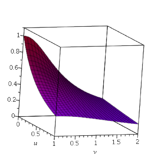
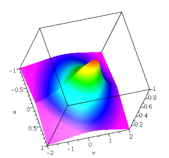
Figure 3: Co-variant meta-conformal two-point function $f$ (4.16). The upper panel shows the quadrant $u\geq 0$, $v\geq 0$, the lower panel shows the scaling function in the entire plane $(u,v)\in\mathbb{R}^{2}$.

The two-point function (4.14) can be written in the scaling form $F(t,z,\bar{z})=t^{-2\delta_{1}}f(z/t,\bar{z}/t)$. Using the algebraic construction described in [60, 61, 62], and restricting to the ‘scalar’ case $\gamma_{1}=\overline{\gamma}_{1}$ for notational simplicity, the scaling function $f(u,v)$ can be extended from the sector $u\geq 0$, $v\geq 0$ to the full plane $(u,v)\in\mathbb{R}$ in the following form (setting $\beta=1$)

$$f(u,v)=\left(\left(1+|u|\right)^{2}+v^{2}\right)^{-2\gamma_{1}}$$ (4.16)

Figure 3 displays $f(u,v)$. The change from the cusp, characteristic for $1D$ meta-conformal symmetry, along the $v=0$ axis to the rounded form of $1D$ otho-conformal symmetry, along the $u=0$ axis, is clearly seen.

In figure 4, the variation of the scaling function (4.16) is shown in polar coordinates, viz. $f=f(r\cos\psi,r\sin\psi)$, over against the length amplitude $r$, for fixed values of the angle $\psi$. The value $\psi=0$ corresponds to the $1D$ meta-conformal case with its characteristic cusp at $r=0$. The value $\psi=\pi/2$ corresponds to the $1D$ ortho-conformal case with is rounded profile near to $r=0$. For larger values of $r$, the decay of the scaling function becomes independent of $\psi$. The other three quadrants look analogously.

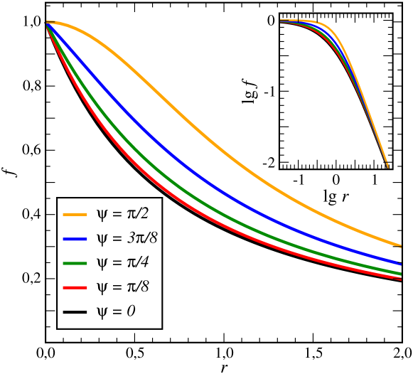
Figure 4: Scaling function (4.16) of the co-variant $2D$ meta-conformal two-point function, in the polar form $f=f(r\cos\psi,r\sin\psi)$ for the angles $\psi=[0,\pi/8,\pi/4,3\pi/8,\pi/2]$ from bottom to top and with $\gamma_{1}=\overline{\gamma}_{1}=\frac{1}{4}$. The inset displays the same function on a doubly logarithmic scale, with ${\rm lg\,}10^{n}=n$.

4.3 The case $p=1/3$

Again, we refer to tables 3 and 4 for the rendering of the canonical coordinates $(\tau,w,\bar{w})$ in terms of the usual time-space coordinates $(t,x,y)$ and the meta-conformal weights. The correspondence between the generators is now as follows

$$A_{n}=\frac{1}{3}X_{n}+\frac{3}{\beta}Y_{n}^{x}\;\;,\;\;B_{n}^{\pm}=X_{n}-\frac{3}{2\beta}Y_{n}^{x}\mp{\rm i}\frac{3}{2\beta}Y_{n}^{y}$$ (4.17)

Once more, the co-variant two-point function is build from the quasi-primary scaling operators $\phi(t,x,y,\gamma,\bar{\gamma})$, where we recall $\gamma=\frac{1}{2}(\gamma_{x}+{\rm i}\gamma_{y})$ and $\bar{\gamma}=\frac{1}{2}(\gamma_{x}-{\rm i}\gamma_{y})$. Taking into the account the covariance of time- and space-translations, we write

$$F=F(t,x,y,\gamma_{1},\gamma_{2},\bar{\gamma}_{1},\bar{\gamma}_{2})=\left\langle\phi(t_{1},x_{1},y_{1},\gamma_{1},\bar{\gamma}_{1})\phi(t_{2},x_{2},y_{2},\gamma_{2},\bar{\gamma}_{2})\right\rangle,$$ (4.18)

where $t=t_{1}-t_{2},x=x_{1}-x_{2},y=y_{1}-y_{2}$. In the canonical coordinates, and writing $\tau=\tau_{1}-\tau_{2}$, $w=w_{1}-w_{2}$ and $\bar{w}=\bar{w}_{1}-\bar{w}_{2}$, the co-variant two-point function reads, up to normalisation

$$F=\tau^{-2\vartheta_{1}}\,w^{-2\Delta_{1}}\,\bar{w}^{-2\overline{\Delta}_{1}}$$ (4.19)

and with the constraints $\vartheta_{1}=\vartheta_{2}$, $\Delta_{1}=\Delta_{2}$ and $\overline{\Delta}_{1}=\overline{\Delta}_{2}$. One may re-express this in the original variables, see table 3, with a qualitative behaviour quite similar to the case $p=-1$ treated above.

5 Application: the directed Glauber-Ising chain

We now discuss how a meta-conformal dynamical symmetry is realised in the relaxational dynamics of the directed Glauber-Ising chain. On an infinitely long chain, Ising spins $\sigma_{n}=\pm 1$ are attached to each site $n$, such that to each configuration $\{\sigma\}$ of spins the energy ${\cal H}[\sigma]=-\sum_{n}\sigma_{n}\sigma_{n+1}$ is associated. The dynamics proceeds through flips of individual spins and is described by a markovian master equation [87]. The rates for a flip of the spin $\sigma_{n}$ is given by [42, 45]

$$w_{n}(\sigma_{n})=\frac{1}{2}\left[1-\frac{\gamma}{2}(1-v)\sigma_{n-1}\sigma_{n}-\frac{\gamma}{2}(1+v)\sigma_{n}\sigma_{n+1}\right]$$ (5.1)

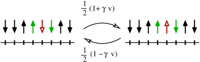
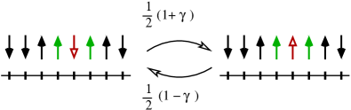
Figure 5: Dependence of the transition rates on the bias $v$ in the directed Glauber-Ising model. The transition rates for flipping the central spin (open arrow, in red) depend on the orientation of its two nearest neighbours (in green). The bias $v$ modifies the rates if (a) the two neighbours have different orientation but cancels if (b) the orientation of the two neighbours is the same.

where $\gamma=\tanh(2/T)$ parametrises the temperature and the left-right bias of the dynamics is described by the parameter $v$. The influence of the parameter $v$ on the transition rates is illustrated in figure 5. Such a directed dynamics does no longer obey the condition of detailed balance, although global balance still holds. Therefore, with the rates (5.1), the equilibrium Gibbs-Boltzmann state is still a stationary state of the dynamics [42]. For either a fully disordered or else a thermalised initial state, the consequences of a non-vanishing bias $v\neq 0$ on the long-time relaxational properties, especially on the precise way how the equilibrium fluctuation-dissipation theorem is broken, have been studied in great detail [42, 45]. Analogous studies have also been carried out in a $2D$ directed kinetic Ising model [44, 46, 47] and the directed $d$-dimensional spherical model [43]. In particular, a $2D$ directed kinetic Ising model quenched to $T=0$ from a fully disordered initial state shows strong evidence for a relaxational behaviour with a dynamical exponent $\mathpzc{z}=1$ [46]. Important observables of interest are the two-time and single-time spin-spin correlators

$$C_{n}(t,s):=\left\langle\sigma_{n}(t)\sigma_{0}(s)\right\rangle\;\;,\;\;C_{n}(t):=C_{n}(t,t)=\left\langle\sigma_{n}(t)\sigma_{0}(t)\right\rangle$$ (5.2)

where spatial translation-invariance will be admitted throughout. At present, we shall merely focus on how a meta-conformal dynamical symmetry is realised in this model. As we shall see, it will be essential to consider initial states with spatially long-ranged correlations, viz. $C_{n}(0)\sim|n|^{-\aleph}$ for $|n|\gg 1$.

From the rates (5.1), the equations of motion of the correlators are readily found [42]

$$\partial_{t}C_{n}(t) =-2(1-\gamma)C_{n}(t)+\gamma\Bigl{(}C_{n-1}(t)+C_{n+1}(t)-2C_{n}(t)\Bigr{)}+\delta_{n,0}\ Z(t)$$ (5.3a)

$$\partial_{\tau}C_{n}(\tau+s,s) =-(1-\gamma)C_{n}(\tau+s,s)+\frac{\gamma}{2}\Bigl{(}C_{n-1}(\tau+s,s)+C_{n+1}(\tau+s,s)-2C_{n}(\tau+s,s)\Bigr{)}$$

$$~{}~{}~{}+\frac{\gamma v}{2}\Bigl{(}C_{n+1}(\tau+s,s)-C_{n-1}(\tau+s,s)\Bigr{)}$$ (5.3b)

where $\tau=t-s$, the Lagrange multiplier $Z(t)$ is fixed by the condition $C_{0}(t)=1$, one has the compatibility condition $C_{n}(t,t)=C_{n}(t)$ and the initial correlator $C_{n}(0)$ must yet be specified.

It is known that the requirement of meta-conformal co-variance determines the scaling form of correlators [62], rather than response functions as it is the case, e.g. for Schrödinger-invariance. Concentrating on the correlators (5.2), from (5.3a) it follows that the single-time correlator $C_{n}(t)$ is independent of the bias $v$ and that one should study the two-time correlators $C_{n}(t,s)$. For illustration, consider first the infinite-temperature limit $\gamma\to 0$ but such that $\gamma v\to\upsilon$ remains finite [45]. Take the continuum limit of (5.3b) and let $C(\tau+s,s;r)=e^{-\tau}\,\mathscr{C}(\tau+s,s;r)$. This gives the equation $\bigl{(}\partial_{\tau}-\upsilon\partial_{r}\bigr{)}\mathscr{C}(\tau+s,s;r)=0$, analogous to (1.11), and with the solution $\mathscr{C}(\tau+s,s;r)=\mathfrak{C}(s;r+\upsilon\tau)$. In the special case $s=0$ of a vanishing waiting time, one has $C(0,0;r)=\mathscr{C}(0,0;r)=\mathfrak{C}(0;r)$. Hence, for a spatially long-ranged initial correlator $C(0,0;r)\sim|r|^{-\aleph}$, with $\aleph>0$, the two-time correlator $C(\tau,0;r)\sim e^{-\tau}(r+\upsilon\tau)^{-\aleph}$ has indeed the form (1.13) predicted by meta-conformal invariance, up to an exponential prefactor.

We now analyse the long-time behaviour in more detail, and for any temperature $T\geq 0$. The equation of motion (5.3b) is solved through a Fourier transformation

$$\widetilde{C}(\tau+s,s;k)=\sum_{n\in\mathbb{Z}}C_{n}(\tau+s,s)\ e^{-{\rm i}nk}\;\;,\;\;C_{n}(\tau+s,s)=\frac{1}{2\pi}\int_{-\pi}^{\pi}\!{\rm d}k\>e^{{\rm i}kn}\>\widetilde{C}(\tau+s,s;k)$$ (5.4)

which in Fourier space leads to

$$\widetilde{C}(\tau+s,s;k)=\widetilde{C}(s;k)\exp\left(-\bigl{[}1-\gamma\cos k-{\rm i}\gamma v\sin k\bigr{]}\tau\right)$$ (5.5)

Tauberian theorems [36] state that the long-time behaviour follows from the form of $\widetilde{C}(\tau+s,s;k)$ around $k\approx 0$. Here, we want to look at a ‘ballistic’ scaling regime where $k\tau$ is being kept fixed, rather than that regime $k^{2}\tau=\mbox{\rm cste.}$ typical for diffusive motion. Indeed, for diffusive scaling, the momenta $k\sim\tau^{-1/2}\gg\tau^{-1}$ are much larger that the ones to be considered here. From now on, we consider a long-ranged initial correlator of the form $C_{n}(0)\sim|n|^{-\aleph}$, for $|n|\to\infty$ and with $\aleph>0$. A simple explicit form [53], which is symmetric in $n$, has the required asymptotic behaviour and is normalised to $C_{0}(0)=1$ reads, along with its Fourier transform [49]

$$C_{n}(0)=\frac{\Gamma\bigl{(}|n|+(1-\aleph)/2\bigr{)}}{\Gamma\bigl{(}|n|+(1+\aleph)/2\bigr{)}}\frac{\Gamma\bigl{(}(1+\aleph)/2\bigr{)}}{\Gamma\bigl{(}(1-\aleph)/2\bigr{)}}\;\;,\;\;\widetilde{C}(0;k)=\frac{\Gamma\bigl{(}(1+\aleph)/2\bigr{)}^{2}}{\Gamma\bigl{(}\aleph\bigr{)}}\left(2\sin\frac{|k|}{2}\right)^{\aleph-1}$$ (5.6)

such that indeed $\widetilde{C}(0;k)\simeq\widetilde{C}_{0}|k|^{\aleph-1}$, for $|k|$ sufficiently small.

(a) The most simple case arises when the waiting time $s=0$. We can directly insert the initial correlator (5.6) into (5.5) and read off the two-point correlator in the requested scaling limit, and for the range $0<\aleph<1$,

$$C_{n}(\tau,0) \simeq \frac{\widetilde{C}_{0}}{2\pi}\int_{\mathbb{R}}\!{\rm d}k\>|k|^{\aleph-1}\left(1-\frac{\gamma}{2}k^{2}\tau+\ldots\right)\ e^{{\rm i}k(n+\gamma v\,\tau)}\,e^{-(1-\gamma)\tau}$$ (5.7)

$$\simeq \frac{\widetilde{C}_{0}\Gamma(\aleph)\cos(\pi\aleph/2)}{\pi}\frac{1}{(n+\gamma v\,\tau)^{\aleph}}\,e^{-(1-\gamma)\tau}$$

$$= \frac{\Gamma\bigl{(}(1+\aleph)/2\bigr{)}^{2}\cos(\pi\aleph/2)}{\pi}\frac{1}{(n+\gamma v\,\tau)^{\aleph}}\,e^{-(1-\gamma)\tau}$$

where the integral is taken from [40, eq. (2.3.12)], see also [26], and (5.6) was used. The unbiased diffusive terms merely lead to corrections to scaling. Eq. (5.7) reproduces indeed the prediction (1.13) of meta-conformal invariance, with $\delta_{1}=\frac{\gamma_{1}}{\mu}=\frac{\aleph}{2}$, and up to an exponentially decaying prefactor and a choice of scale of spatial distances. Clearly, both the bias $v\neq 0$ as well as long-ranged initial conditions with $0<\aleph<1$ are necessary ingredients for the meta-conformal dynamical symmetry to arise.

(b) For arbitrary waiting times $s>0$, we must now show, under suitable conditions and at least for $s$ sufficiently large and for $|k|$ sufficiently small, that $\widetilde{C}(s;k)\simeq\widetilde{\mathscr{C}}(s)|k|^{\aleph-1}$. If that is so, then the two-time correlator $C_{n}(\tau+s,s)$, see eq. (5.5), will be of the same form as in (5.7), with a prefactor $\widetilde{\mathscr{C}}(s)$ which might still depend on the waiting time $s$.

The proof of this property requires to solve (5.3a). Define the Laplace transform $\widetilde{\overline{C}}(p;k):=\int_{0}^{\infty}\!{\rm d}t\>e^{-ps}\>\widetilde{C}(s;k)$. The solution of (5.3a) reads in Laplace-Fourier space

$$\widetilde{\overline{C}}(p;k)=\frac{\overline{Z}(p)+\widetilde{C}(0;k)}{p+2(1-\gamma\cos k)}$$ (5.8)

The Lagrange multiplier $\overline{Z}(p)$ is found from the condition $\overline{C}_{0}(p)=1/p$. Explicitly

$$\frac{1}{p}=\frac{1}{2\pi}\int_{-\pi}^{\pi}\!{\rm d}k\>\left[\frac{\overline{Z}(p)}{p+2(1-\gamma\cos k)}+\frac{\widetilde{C}(0;k)}{p+2(1-\gamma\cos k)}\right]$$ (5.9)

Herein, the first integral can be taken from [42]. To analyse the second integral, we use again the explicit form (5.6) and consider the leading small-$p$ behaviour of

$$J(p;\gamma,\aleph):=\frac{\Gamma\bigl{(}(1+\aleph)/2\bigr{)}^{2}}{\pi\Gamma\bigl{(}\aleph\bigr{)}}\int_{0}^{\pi}\!{\rm d}k\>\frac{\bigl{(}2\sin k/2\bigr{)}^{\aleph-1}}{p+2(1-\gamma\cos k)}\stackrel{{\scriptstyle p\to 0}}{{\simeq}}\left\{\begin{array}[]{ll}J(0;\gamma,\aleph)&\mbox{\rm~{}~{};~{} if $\gamma<1$}\\ J_{\infty}\,p^{\aleph/2-1}&\mbox{\rm~{}~{};~{} if $\gamma=1$}\end{array}\right.$$ (5.10)

where $J_{\infty}=\left.\Gamma\bigl{(}(1+\aleph)/2\bigr{)}\Gamma\bigl{(}1-\aleph/2\bigr{)}\right/2^{\aleph}\sqrt{\pi\,}$. For $\gamma<1$, $J(0;\gamma,\aleph)$ is a finite constant. From the constraint (5.9), and since $\aleph>0$, this implies for the leading small-$p$ behaviour of the Lagrange multiplier

$$\overline{Z}(p) = \bigl{(}p+2(1-\gamma)\bigr{)}^{1/2}\bigl{(}p+2(1+\gamma)\bigr{)}^{1/2}\left(\frac{1}{p}-J(p;\gamma,\aleph)\right)$$ (5.13)

$$\stackrel{{\scriptstyle p\to 0}}{{\simeq}} \left\{\begin{array}[]{ll}2\sqrt{1-\gamma^{2}\,}\,p^{-1}\bigl{(}1+{\rm o}(p)\bigr{)}&\mbox{\rm~{}~{};~{} if $\gamma<1$}\\[3.41418pt] 2\,p^{-1/2}\hskip 37.55785pt\bigl{(}1+{\rm o}(p)\bigr{)}&\mbox{\rm~{}~{};~{} if $\gamma=1$}\end{array}\right.$$

where the estimates (5.10) for $J(p;\gamma,\aleph)$ were used. We see that the leading behaviour of $\overline{Z}(p)$ is independent of the initial condition.

Using (5.13), we now examine the correlator (5.8) in the asymptotic double limit $p\to 0$ and $k\to 0$. Because of the dynamical exponent $\mathpzc{z}=1$ of meta-conformal invariance, we expect that this limit should be taken such that $p/k$ is being kept fixed. First, for $\gamma<1$, we find

$$\widetilde{\overline{C}}(p;k)\simeq\frac{2\sqrt{1-\gamma^{2}\,}\,p^{-1}+\widetilde{C}_{0}|k|^{\aleph-1}}{2(1-\gamma)+{\rm O}(p,k^{2})}\simeq\sqrt{\frac{1+\gamma}{1-\gamma}\,}\,p^{-1}\bigl{(}1+{\rm o}(1)\bigr{)}\;\;;\;\;\mbox{\rm if $\gamma<1$}$$ (5.14)

because for $\aleph>0$, the second term in the numerator is less singular than the first one. Hence, going back to sufficiently long waiting times $s\gg 1$, we obtain $\widetilde{C}(s;k)\simeq\sqrt{\frac{1+\gamma}{1-\gamma}\,}$ which is constant and independent of the long-range initial conditions. Hence for $\gamma<1$ there is no meta-conformal invariance of the two-time correlator in the limit of large waiting times. Second, for $\gamma=1$ we have instead

$$\widetilde{\overline{C}}(p;k)\simeq\frac{2\,p^{-1/2}+\widetilde{C}_{0}|k|^{\aleph-1}}{p+k^{2}}\simeq\left\{\begin{array}[]{ll}\frac{\Gamma\bigl{(}(1+\aleph)/2\bigr{)}^{2}}{\Gamma\bigl{(}\aleph\bigr{)}}\frac{|k|^{\aleph-1}}{p}&\mbox{\rm~{}~{};~{} if $\aleph<\frac{1}{2}$}\\[14.22636pt] 2\,p^{-3/2}&\mbox{\rm~{}~{};~{} if $\aleph>\frac{1}{2}$}\end{array}\right.\;\;,\;\;\mbox{\rm and if $\gamma=1$}$$ (5.15)

Hence, if $\aleph<\frac{1}{2}$, we have the leading long-time behaviour $\widetilde{C}(s;k)\simeq\widetilde{C}_{0}|k|^{\aleph-1}$, with $\widetilde{C}_{0}$ given in (5.6), for the single-time correlator. We have therefore verified a sufficient condition that the form of the two-time correlator $C_{n}(\tau+s,s)$ is in agreement with the expected form (1.13) of meta-conformal invariance. On the other hand, if $\aleph>\frac{1}{2}$, no clear evidence for such an invariance is found. Therefore, for large waiting times $s\to\infty$, meta-conformal invariance of the two-time correlator can only be established under more restrictive conditions than for $s=0$ (or $s$ finite and sufficiently small).

We summarise the results of this section as follows.

Proposition 10: At zero temperature $T=0$, the two-time spin-spin correlator $C_{n}(\tau,s)$ in the directed Glauber-Ising chain, with long-ranged initial correlators of the form $C_{n}(0)\sim|n|^{-\aleph}$ with $0<\aleph<\frac{1}{2}$, takes for large waiting times $s\gg 1$ and large time differences $\tau=t-s\gg 1$ the form (1.13), predicted by meta-conformal invariance.

While we gave here an example of $1D$ meta-conformal invariance, we point out that the Lie algebra of $2D$ meta-conformal transformations is isomorphic to the dynamical symmetry [64] of the spatially non-local stochastic process of $1D$ diffusion-limited erosion [72] or the terrace-step-kink model [83, 71].

6 Conclusions

We have explored the construction of time-space transformations, with a dynamical exponent $\mathpzc{z}=1$, which may have physical applications as dynamical symmetries. Ortho-conformal transformations have been the well-known standard example of such transformations, with spectacular applications to conformal field-theory, especially in $2D$ equilibrium phase transitions. Our main result is stated in table 1: there are infinite-dimensional Lie groups of time-space transformations, both for $d=1$ and $d=2$, which contain the same temporal and spatial translations as well as dilatations, as the orthoconformal group, yet these transformations are in general not angle-preserving and hence cannot be ortho-conformal. The relationship between ortho- and meta-conformal transformation for any $d$ is stated in (3.10). The $1D$ meta-conformal case illustrates the interest in working with representations of the conformal group which uses non-orthogonal coordinates. For the $2D$ case, the associated Lie algebra is isomorphic to the direct sum of three Virasoro algebras, rather than two as one is used to from $2D$ ortho-conformal invariance. Tables 2, 3 and 4 show how the generic generators (4.3) are related to the physically motivated time-space transformations.

The meta-conformal transformations as constructed here are well-known to act as dynamical symmetries of a simple linear equation of ballistic transport. A new class of applications has been described here: the long-time, large-distance relaxation of non-equilibrium spin systems whose dynamics contains a directional bias. If in addition sufficiently long-ranged initial spatial correlations occur, then the dynamical scaling regime with $\mathpzc{z}=1$ is described by meta-conformal invariance. We have shown this explicitly for the two-time spin-spin correlator of the directed Glauber-Ising chain, at vanishing temperature and for a decay exponent $0<\aleph<\aleph_{c}=\frac{1}{2}$ of the initial spin-spin correlator $C_{n}(0)\sim|n|^{-\aleph}$.

While this kind of application merely uses the finite-dimensional sub-algebra of meta-conformal invariance, the full theory based on the infinite-dimensional symmetry remains to be constructed. On the other hand, one still must demonstrate that meta-conformal symmetries arise in systems which are not described by linear equations of motion. Previous experience from the phase-ordering kinetics of non-equilibrium spin systems (where $\mathpzc{z}=2$), provides evidence that dynamical Schrödinger-invariance applies generically [58], for example to kinetic Ising and Potts models, although the Schrödinger group was originally constructed as the dynamical symmetry of the free diffusion equation. Therefore, by analogy a naturally-looking path for identifying meta-conformally invariant systems appears to be the study of directed spin systems in $d>1$ spatial dimensions. Our results on the Glauber-Ising chain suggest that meta-conformal invariance might be found for directed systems quenched to temperatures $T\leq T_{c}$, that is below or onto the critical temperature $T_{c}$. The existence of dynamical scaling with $\mathpzc{z}=1$ in such higher-dimensional models has already been demonstrated [46].

Acknowledgements: We warmly thank the organisers of the 10^th International Symposium “Quantum Theory and Symmetries” and of the atelier “Lie Theory and Applications in Physics XII” in Varna (June 2017) for the excellent atmosphere, where the main idea for this work arose. MH gratefully thanks H. Herrmann and his group “Rechnergestützte Physik der Werkstoffe” at the Institut für Baustoffe (IfB) at ETH Zürich (Switzerland) for warm hospitality during a sabbatical year 2016/17, where many of the ideas presented here were conceived. This work was supported by PHC Rila and by Bulgarian National Science Fund Grant KP-06-N28/6.

References

- [1] N. Aizawa, Z. Kuznetsova, F. Toppan, Invariant partial differential equations with two-dimensional exotic centrally extended conformal Galilei symmetry, J. Math. Phys. 57, 041701 (2016), [arXiv:1512.02290].
- [2] F.C. Alcaraz, V. Rittenberg, Nonlocal growth processes and conformal invariance, J. Stat. Mech. P05022 (2012), [arXiv:arXiv:1204.1001].
- [3] F.C. Alcaraz, V. Rittenberg, Nonlocal asymmetric exclusion process on a ring and conformal invariance, J. Stat. Mech. P09010 (2013), [arXiv:1305.4522].
- [4] F.C. Alcaraz, V. Rittenberg, Correlation functions in conformal invariant stochastic processes, J. Stat. Mech. P11012 (2015), [arXiv:1508.06968].
- [5] A. Bagchi, R. Gopakumar, Galilean conformal algebras and AdS/CFT, JHEP 0907:037 (2009), [arXiv:0902.1385].
- [6] A. Bagchi, R. Gopakumar, I. Mandal, A. Miwa, CGA in 2D, JHEP 1008:004 (2010), [arXiv:0912.1090].
- [7] A. Bagchi, S. Detournay, R. Fareghbal, J. Simón, Holographies of flat cosmological horizons, Phys. Rev. Lett. 110, 141302 (2013) [arxiv:1208.4372]
- [8] A. Bagchi, M. Gary, Zodinmawia, Bondi-Metzner-Sachs bootstrap, Phys. Rev. D96, 025007 (2017), [arxiv:1612:01730].
- [9] G. Barnich and G. Compère, Classical central extension for asymptotic symmetries at null infinity in three spacetime dimensions, Class. Quant. Grav. 24 F15 (2007); corrigendum 24, 3139 (2007) [gr-qc/0610130].
- [10] G. Barnich, A. Gomberoff, H.A. González, Three-dimensional Bondi-Metzner-Sachs invariant two-dimensional field-theories as the flat limit of Liouville theory, Phys. Rev. D87, 124032 (2007), [arxiv:1210.0731].
- [11] A.A. Belavin, A.M. Polykaov, A.B. Zamolodchikov, Infinite conformal symmetry in two-dimensional quantum field-theory, Nucl. Phys. B241, 333 (1984).
- [12] B. Bertini, M. Collura, J. de Nardis, M. Fagotti, Transport in out-of-equilibrium XXZ chains: exact profiles of charges and currents, Phys. Rev. Lett. 117, 207201 (2016), [arXiv:1605.09790].
- [13] G.W. Bluman, J.D. Cole, The general similarity solution of the heat equation, J. Math. Mech. 18, 1025 (1969).
- [14] H. Bondi, M.G.J. van der Burg, A.W.K. Metzner, Gravitational waves in general relativity, Proc. Roy. Soc. London, A269, 21 (1962).
- [15] G. Burdet, M. Perrin, Many-body realization of the Schrödinger algebra, Lett. Nuov. Cim. 4, 651 (1972).
- [16] P. Calabrese, J.L. Cardy, Entanglement and correlation functions following a local quench: a conformal field theory approach, J. Stat. Mech. P10004 (2007), [arXiv:0708.3750].
- [17] P. Calabrese, J.L. Cardy, Quantum quenches in 1+1 dimensional conformal field theories, J. Stat. Mech. P064003 (2016), [arXiv:1603.02889].
- [18] A. Campa, T. Dauxois, S. Ruffo, Statistical mechanics and dynamics of solvable models with long-range interactions, Phys. Rep. 480, 57-159 (2009) [arXiv:0907.0323].
- [19] A. Campa, T. Dauxois, D. Fanelli, S. Ruffo, Physics of Long-Range Interacting Systems (Oxford University Press, Oxford, England 2014).
- [20] A. Cappelli, G.V. Dunne, C.A. Trugenberger, G.R. Zemba, Conformal symmetry and universal properties of quantum Hall states, Nucl. Phys. B398, 531 (1993), [arXiv:hep-th/9211071].
- [21] J.L. Cardy, Conformal invariance and critical dynamics, J. Phys. A18, 2271 (1985).
- [22] O.A. Castro-Alvaredo, B. Doyon, T. Yoshimura, Emergent hydrodynamics in integrable quantum systems out of equilibrium, Phys. Rev. X6, 041065 (2016), [arXiv:1605.07331].
- [23] J.-S. Caux, B. Doyon, J. Dubail, R. Konik, T. Yoshimura, Hydrodynamics of the interacting Bose gas in the Quantum Newton Cradle setup, [arXiv:1711.00873].
- [24] R. Cherniha, M. Henkel, The exotic conformal Galilei algebra and nonlinear partial differential equations, J. Math. Anal. Appl. 369, 120 (2010) [arXiv:0910.4822].
- [25] R. Cherniha, V. Davydovych, Nonlinear reaction-diffusion systems, Springer Lecture Notes in Mathematics LNM 2196, Springer (Heidelberg 2017).
- [26] E.T. Copson, Asymptotic expansions, Cambridge Univ. Press (Cambridge 1965).
- [27] N. Crampe, E. Ragoucy, V. Rittenberg, M. Vanicat, Integrable dissipative exclusion process: Correlation functions and physical properties, Phys. Rev. E94, 032102 (2016), [arXiv:1603.06796].
- [28] G. Delfino, Correlation spreading and properties of the quantum state in quench dynamics, Phys. Rev. E97, 062138 (2018), [arXiv:1710.06275].
- [29] B. Doyon, J. Dubail, R. Konik, T. Yoshimura, Large-scale description of interacting one-dimensional Bose gases: generalized hydrodynamics supersedes conventional hydrodynamics, [ arXiv:1704.04151].
- [30] J. Dubail, A more efficient way to describe interacting quantum particles in , Physics 9, 153 (2016).
- [31] A. Dutta, G. Aeppli, B.K. Chakrabarti, U. Divakaran, T.F. Rosenbaum, D. Sen, Quantum phase transitions in transverse-field spin models, Cambridge University Press (Cambridge 2015).
- [32] C. Duval, P.A. Horváthy, Non-relativistic conformal symmetries and Newton-Cartan structures, J. Phys. A: Math. Theor. 42, 465206 (2009), [arXiv:0904.0531].
- [33] C. Duval, G.W. Gibbons, P.A. Horváthy, Conformal Carroll groups, J. Phys. A: Math. Theor. 47, 335204 (2014), [arXiv:1403.4213].
- [34] C. Duval, G.W. Gibbons, P.A. Horváthy, Conformal Carroll groups and BMS symmetry, Class. Quantum Gravity 34, 092001 (2014), [arXiv:1402.5894].
- [35] Y. Elskens, D. Escande, F. Doveil, Vlasov equation and -body dynamics, Eur. Phys. J. D68, 218 (2014) [arxiv:1403.0056].
- [36] W. Feller, An introduction to probability theory and its applications, vol. 2 (2nd ed), Wiley (New York 1971).
- [37] P. di Francesco, P. Mathieu, D. Sénéchal, Conformal field theory, Springer (Heidelberg 1997).
- [38] V.I. Fushchych, M.I. Serov, V.I. Chopyk, Conditional invariance and nonlinear heat equations, Proc. Acad. Sci. Ukr. 9, 17 (1988) [in russian]
- [39] W. Fushchych, W.M. Shtelen, M. Serov, Symmetry analysis and exact solutions of equations of nonlinear mathematical physics, Kluwer (Dordrecht 1993).
- [40] I.M. Gelfand, G.E. Shilov, Generalised functions, vol. 1, Academic Press (London 1964).
- [41] P.-G. de Gennes, Scaling concepts in polymer physics, Cornell Univ. Press (Ithaca 1979).
- [42] C. Godrèche, Dynamics of the directed Ising chain, J. Stat. Mech. P04005 (2011) [arxiv:1102.0141.
- [43] C. Godrèche, J.-M. Luck, Asymmetric Langevin dynamics for the ferromagnetic spherical model, J. Stat. Mech. P05006 (2013) [arxiv:1302.4658].
- [44] C. Godrèche, M. Pleimling, Dynamics of the two-dimensional directed Ising model in the paramagentic phase, J. Stat. Mech. P05005 (2014) [arXiv:1401.1988].
- [45] C. Godrèche, J.-M. Luck, Single spin-flip dynamics of the Ising chain, J. Stat. Mech. P05033 (2015) [arxiv:1503.01661].
- [46] C. Godrèche, M. Pleimling, Dynamics of the two-dimensional directed Ising model: zero-temperature coarsening, J. Stat. Mech. P07023 (2015) [arxiv:1505.06587].
- [47] C. Godrèche, M. Pleimling, Freezing in stripe states for kinetic Ising models: a comparative study of three dynamics, J. Stat. Mech. 043209 (2018) [arxiv:1801.07749].
- [48] C.R. Hagen, Scale and conformal transformations in Galilean-covariant field-theory, Phys. Rev. D5, 377 (1972).
- [49] E.R. Hansen, A table of series and products, Prentice Hall (Englewood Cliffs 1975).
- [50] T.H. Hansson, M. Hermanns, S.H. Simon, S.F. Viefers, Quantum Hall physics: hierarchies and conformal field-theory techniques, Rev. Mod. Phys. 89, 025005 (2017), [arXiv:1601.01697].
- [51] P. Havas and J. Plebanski, Conformal extensions of the Galilei group and their relation to the Schrödinger group, J. Math. Phys. 19, 482 (1978).
- [52] M. Henkel, Schrödinger-invariance and strongly anisotropic critical systems, J. Stat. Phys. 75, 1023 (1994), [arxiv:hep-th/9310081].
- [53] M. Henkel, D. Karevski, Lattice two-point functions and conformal invariance, J. Phys. A Math. Gen. 31, 2503 (1998) [arxiv:cond-mat/9711265].
- [54] M. Henkel, Conformal invariance and critical phenomena, Springer (Heidelberg 1999).
- [55] M. Henkel, Phenomenology of local scale-invariance: from conformal invariance to dynamical scaling, Nucl. Phys. B641, 405 (2002) [hep-th/0205256].
- [56] M. Henkel, J. Unterberger, Schrödinger invariance and space-time symmetries, Nucl. Phys. B660, 407 (2003) [hep-th/0302187].
- [57] M. Henkel, G.M. Schütz, On the universality of the fluctuation-dissipation ratio in non-equilibrium critical dynamics, J.Phys. A Math. Gen. 37, 591 (2004) [arxiv:cond-mat/0308466].
- [58] M. Henkel, M. Pleimling, Non-equilibrium phase transitions vol. 2: ageing and dynamical scaling far from equilibrium (Springer, Heidelberg, Germany 2010).
- [59] M. Henkel, Causality from dynamical symmetry: an example from local scale-invariance, in A. Makhlouf et al. (eds.), Algebra, Geometry and Mathematical Physics, Springer Proc. Math. & Statistics 85, 511 (2014), [arxiv:1205.5901].
- [60] M. Henkel, Dynamical symmetries and causality in non-equilibrium phase transitions, Symmetry 7, 2108 (2015), [arxiv:1509.03669].
- [61] M. Henkel, S. Stoimenov, Physical ageing and Lie algebras of local scale-invariance, in V. Dobrev (ed) Lie Theory and its Applications in Physics, Springer Proc. Math. & Statizstics 111, 33 (2015) [arxiv:1401.6086].
- [62] M. Henkel and S. Stoimenov, Meta-conformal invariance and the boundedness of two-point correlation functions. J. Phys A: Math. Theor. 49, 47LT01 (2016), [arxiv:1607.00685].
- [63] M. Henkel, Non-local meta-conformal invariance in diffusion-limited erosion, J. Phys. A Math. Theor. 49, 49LT02 (2016) [arxiv:1606.06207].
- [64] M. Henkel, Non-local meta-conformal invariance, diffusion-limited erosion and the XXZ chain, Symmetry 9, 2 (2017) [arxiv:1611.02975].
- [65] M. Henkel, From dynamical scaling to local scale-invariance: a tutorial, Eur. Phys. J. Spec. Topics 226, 605 (2017), [arxiv:1610.06122].
- [66] M. Hénon, Vlasov equation ?, Astron. Astrophys. 114, 211 (1982).
- [67] A. Hosseiny, S. Rouhani, Affine extension of Galilean conformal algebra in 2+1 dimensions, J. Math. Phys. 51, 052307 (2010) [arxiv:0909.1203].
- [68] R. Jackiw, Introducing scale symmetry, Phys. Today 25, 23 (1972).
- [69] C.G. Jacobi, Vorlesungen über Dynamik, 4. Vorlesung (Königsberg 1842/43), in A. Clebsch, A. Lottner (eds), Gesammelte Werke von C.G. Jacobi, Akademie der Wissenschaften (Berlin 1866/1884).
- [70] J.H. Jeans, On the theory of star-streaming and the structure of the universe, Monthly Notices Roy. Astron. Soc. 76, 70 (1915).
- [71] D. Karevski, G.M. Schütz, Conformal invariance in driven diffusive systems at high currents, Phys. Rev. Lett. 118, 030601 (2017), [arXiv:1606.04248.
- [72] J. Krug, P. Meakin, Kinetic roughening of laplacian fronts, Phys. Rev. Lett. 66, 703 (1991).
-
[73]
S. Lie,
Über die Integration durch bestimmte Integrale von einer Klasse linearer partieller Differentialgleichungen,
Arch. Math. Naturvidenskap. (Kristiania) 6, 328 (1881);
S. Lie, Vorlesungen über Differentialgleichungen mit bekannten infinitesimalen Transformationen, Teubner (Leipzig 1891). - [74] A. Maraga, A. Chiocchetta, A. Mitra, A. Gambassi, Ageing and coarsening in isolated quantum systems after a quench: exact results for the quantum -model with , Phys. Rev. E92, 042151 (2015) [arXiv:1506.04528].
- [75] D. Martelli, Y. Tachikawa, Comments on Galilean conformal field theories and their geometric realization, JHEP 1005:091 (2010), [arXiv:0903.5184].
- [76] H. Mo, F. van den Bosch, S. White, Galaxy formation and evolution (Cambridge University Press, Cambridge, England 2010).
- [77] U. Niederer, The maximal kinematical invariance group of the free Schrödinger equation, Helv. Phys. Acta 45, 802 (1972).
- [78] L. Piroli, J. de Nardis, M. Collura, B. Bertini, M. Fagotti, Transport in out-of-equilibrium XXZ chains: Nonballistic behaviour and correlation functions, Phys. Rev. B96, 115124 (2017), [arXiv:1706.00413].
- [79] J. Polchinski, String theory (2 vols.), Cambridge University Press (Cambridge 2001).
- [80] F. Pegoraro, F. Califano, G. Manfredi, P.J. Morrison, Theory and applications of the Vlassov equation, Eur. Phys. J. D69, 68 (2015) [arXiv:1502.03768].
- [81] S. Rychkov, EPFL lectures on conformal field theory in dimensions, Springer (Heidelberg 2017).
- [82] G.M. Schütz, Conformal invariance in conditioned stochastic particle systems, J. Phys. A50, 314002 (2017).
- [83] H. Spohn, Bosonization, vicinal surfaces, and hydrodynamic fluctuation theory, Phys. Rev. E60, 6411 (1999) [arxiv:cond-mat/9908381].
- [84] S. Stoimenov and M. Henkel, From conformal invariance towards dynamical symmetries of the collisionless Boltzmann equation, Symmetry 7, 1595 (2015) [arxiv:1509.00434].
- [85] S. Stoimenov and M. Henkel, Construction of meta-conformal algebras in spatial dimensions, AIP Conf. Proc. 2075, 090026 (2019).
- [86] U.C. Täuber, Critical dynamics, Cambridge University Press (Cambridge 2014).
- [87] T. Tomé, M.J. de Oliveira, Dinâmica estocástica e irreversibilidade, 2a ed., Editora Edusp (São Paulo 2014).
- [88] J. Unterberger, C. Roger, The Schrödinger-Virasoro algebra: mathematical structure and dynamical Schrödnger symmetries, Springer (Heidelberg 2012).
- [89] C. Vilani, Particle systems and non-linear Landau damping, Phys. Plasmas 21, 030901 (2014).
- [90] A.A. Vlasov, On vibration properties of electron gas (in Russian), Sov. Phys. JETP, 8, 291 (1938).
- [91] S. Wald, G.T. Landi, M. Henkel, Lindblad dynamics of the quantum spherical model, J. Stat. Mech. 013103 (2018) [arxiv:1707:06273].
- [92] P.-M. Zhang and P.A. Horváthy, Non-relativistic conformal symmetries in fluid mechanics, Eur. Phys. J. C65, 607 (2010).