Revisiting the mechanical properties of the nucleon

Abstract

We discuss in detail the distributions of energy, radial pressure and tangential pressure inside the nucleon. In particular, this discussion is carried on in both the instant form and the front form of dynamics. Moreover we show for the first time how these mechanical concepts can be defined when the average nucleon momentum does not vanish. We express the conditions of hydrostatic equilibrium and stability in terms of these two and three-dimensional energy and pressure distributions. We briefly discuss the phenomenological relevance of our findings with a simple yet realistic model. In the light of this exhaustive mechanical description of the nucleon, we also present several possible connections between hadronic physics and compact stars, like e.g. the study of the equation of state for matter under extreme conditions and stability constraints.

I Introduction

Understanding how quarks and gluons bind together to form nucleons is a challenging and formidable open problem. Since a couple of decades, one of the main focuses of hadronic physics consists in the study of the mass and spin structure of the nucleon. This information is encoded in the energy-momentum tensor (EMT) which can be probed in various high-energy exclusive scattering experiments Ji:1996ek ; Ji:1996nm . Since the corresponding cross-sections are small, these processes are studied in high-luminosity setups like Jefferson Laboratory or COMPASS at CERN, and constitute an important aspect of the experimental program to be conducted in a near future in a U.S.-based Electron-Ion Collider Accardi:2012qut . The nucleon EMT is also intensively studied using Lattice QCD, see Yang:2018bft ; Alexandrou:2018xnp ; Yang:2018nqn ; Shanahan:2018pib ; Shanahan:2018nnv for recent developments.

Beside mass and spin, the EMT is also a fundamental object encoding mechanical properties of the nucleon like stress Pais:1949vdk ; Polyakov:2002yz ; Polyakov:2018zvc . Unlike ordinary media at equilibrium, the stress inside the nucleon is not isotropic. Indeed, some theoretical investigations Ruderman:1972aj ; Canuto:1974ft already showed that the nuclear matter itself may become anisotropic at very high densities ($>10^{15}$ g/cm³), where the nuclear interactions must be treated relativistically. Such conditions are typically met inside compact stars which cannot be explained properly in terms of an ordinary equation of state (EoS) Alcock:1986hz ; Haensel:1986qb ; Weber:2004kj ; PerezGarcia:2010ap ; Rodrigues:2011zza . Stress anisotropy in self-gravitating systems has been studied in Bowers:1974tgi ; Herrera:1997plx ; Mak:2001eb and has been shown to affect the physical properties, stability and structure of stellar matter Dev:2000gt ; Dev:2003qd ; Silva:2014fca . In particular, anisotropic stellar objects can be much more compact than the isotropic ones Boehmer:2006ye . In the chiral quark-soliton model Goeke:2007fp , it has been found that the energy density at the center of the nucleon is about $3\times 10^{15}$ g/cm³, i.e. 13 times higher than the average density of nuclear matter. It is therefore no wonder that stress anisotropy plays a significant role in the mechanical structure of the nucleon.

So far, the mechanical properties of the nucleon have been studied in the Breit frame based on the symmetric Belinfante-Rosenfeld form of the EMT Polyakov:2002yz ; Goeke:2007fp . It is known however that distributions defined in the Breit frame are subject to relativistic corrections Burkardt:2002hr and that the spin of the constituents makes the nucleon EMT asymmetric Leader:2013jra ; Lorce:2017wkb . In view of this, we propose a detailed revisit of the mechanical structure of the nucleon addressing the above shortcomings.

The paper is organized as follows. In Section II we explain how to describe a relativistic quantum system localized in phase space and present the matrix elements of the general asymmetric EMT. Mechanical properties of the nucleon defined in the instant form of dynamics are discussed in Section III. After a quick review of the proper decomposition of the nucleon EMT into quark and gluon contributions, we present the three-dimensional spatial distributions defined in the Breit frame where the system is in average at rest. We extend the study to the more general class of elastic frames introduced in Lorce:2017wkb , where two-dimensional spatial distributions can be defined in the plane transverse to the average motion of the system. In Section IV, we discuss for the first time the mechanical structure of the nucleon using the front form of dynamics. In such a framework, we define two-dimensional spatial distributions free of relativistic corrections and compare them with the corresponding distributions in instant form. The questions of hydrostatic equilibrium and stability conditions are discussed in Section V. Finally, we conclude the paper with Section VI where we summarize our results.

II Matrix elements of the energy-momentum tensor

In order to define the distribution of a physical quantity inside a system, one should first localize the system in both position and momentum space. In a quantum theory, this can be achieved in the Wigner sense Hillery:1983ms . A system with average position $R$ and average momentum $P$ is described by the covariant phase-space density operator

$$\rho_{R,P}=\int\frac{\mathrm{d}P^{2}}{2\pi}\int\frac{\mathrm{d}^{4}\Delta}{(2\pi)^{4}}\,2\pi\,\delta(2P\cdot\Delta)\,2\pi\,\delta(P^{2}+\tfrac{\Delta^{2}}{4}-M^{2})\,e^{-i\Delta\cdot R}\,{\left|P-\tfrac{\Delta}{2}\right\rangle}{\left\langle P+\tfrac{\Delta}{2}\right|}\,,$$ (1)

where the delta functions ensure that initial and final states have the same mass $M$. It follows from the relativistic normalization for momentum eigenstates $\langle p^{\prime}|p\rangle=2p^{0}(2\pi)^{3}\,\delta^{(3)}(\boldsymbol{p}^{\prime}-\boldsymbol{p})$ that $\mathrm{Tr}[\rho_{R,P}]=1$. Defining the covariant “position” states as

$${\left|x\right\rangle}=\int\frac{\mathrm{d}^{4}p}{(2\pi)^{4}}\,2\pi\,\delta(p^{2}-M^{2})\,e^{ip\cdot x}\,{\left|p\right\rangle}\,,$$ (2)

with normalization $\langle x^{\prime}|x\rangle=\int\frac{\mathrm{d}^{3}p}{(2\pi)^{3}2p^{0}}\,e^{-ip\cdot(x^{\prime}-x)}$, the covariant phase-space density operator can alternatively be expressed as

$$\rho_{R,P}=\int\frac{\mathrm{d}P^{2}}{2\pi}\int\mathrm{d}^{4}Z\,e^{-iP\cdot Z}\,{\left|R+\tfrac{Z}{2}\right\rangle}{\left\langle R-\tfrac{Z}{2}\right|}\,.$$ (3)

If we integrate the covariant phase-space density operator over the position $\boldsymbol{R}$, we recover the density operator in momentum space

$$\int\mathrm{d}^{3}\boldsymbol{R}\,\rho_{R,P}=\int\frac{\mathrm{d}P^{2}}{2\pi}\,2\pi\,\delta(P^{2}-M^{2})\,\frac{{\left|P\right\rangle}{\left\langle P\right|}}{2P^{0}}\,,$$ (4)

and if we integrate over the momentum $\boldsymbol{P}$, we recover the density operator in position space

$$\int\frac{\mathrm{d}^{3}\boldsymbol{P}}{(2\pi)^{3}2P^{0}}\,\rho_{R,P}={\left|R\right\rangle}{\left\langle R\right|}\,.$$ (5)

Matrix elements of position-dependent operators are then given by

$$\langle O(X)\rangle_{R,P}=\mathrm{Tr}[O(X)\rho_{R,P}]\,,$$ (6)

and translation invariance implies that

$$\langle O(X)\rangle_{R,P}=\langle O(x)\rangle_{0,P}\,,$$ (7)

where $x=X-R$ is the relative average position.

In the present work, we are interested in matrix elements of the (renormalized) nucleon EMT $T^{\mu\nu}(X)$. The latter can be expressed in terms of gravitational (or energy-momentum) form factors (GFFs), first introduced by Kobzarev and Okun Kobzarev:1962wt ; Kobzarev:1962wt2 and later by Pagels Pagels:1966zza . In the general case of a local, gauge-invariant asymmetric EMT for a spin-$\frac{1}{2}$ target, the standard parametrization reads Bakker:2004ib ; Leader:2013jra ; Lorce:2015lna ; Lorce:2017wkb

$${\left\langle p^{\prime},\boldsymbol{s}^{\prime}\right|}T^{\mu\nu}_{a}(0){\left|p,\boldsymbol{s}\right\rangle}=\bar{u}(p^{\prime},\boldsymbol{s}^{\prime})\Bigg{\{} \frac{P^{\mu}P^{\nu}}{M}\,A_{a}(t)+\frac{\Delta^{\mu}\Delta^{\nu}-\eta^{\mu\nu}\Delta^{2}}{M}\,C_{a}(t)+M\eta^{\mu\nu}\bar{C}_{a}(t)$$ (8)

$$+\frac{P^{\{\mu}i\sigma^{\nu\}\Delta}}{4M}\left[A_{a}(t)+B_{a}(t)\right]+\frac{P^{[\mu}i\sigma^{\nu]\Delta}}{4M}\,D_{a}(t)\Bigg{\}}u(p,\boldsymbol{s})\,,$$

where $p$ ($p^{\prime}$) and $\boldsymbol{s}$ ($\boldsymbol{s}^{\prime}$) are the four-momentum and canonical polarization of the initial (final) nucleon of a mass $M$, $\eta^{\mu\nu}=\text{diag}(+,-,-,-)$ is the Minkowski metric, and $t=\Delta^{2}$ with $\Delta=p^{\prime}-p$ and $P=(p^{\prime}+p)/2$. For convenience, we introduced the symmetrizer $a^{\{\mu}b^{\nu\}}=a^{\mu}b^{\nu}+a^{\nu}b^{\mu}$, the antisymmetrizer $a^{[\mu}b^{\nu]}=a^{\mu}b^{\nu}-a^{\nu}b^{\mu}$, and the notation $i\sigma^{\mu\Delta}=i\sigma^{\mu\lambda}\Delta_{\lambda}$. The label $a$ in Eq. (8) refers to the contribution from a particular type of constituents, typically $a=q$ for quarks and $a=G$ for gluons, here defined in the $\overline{\text{MS}}$ scheme . The total EMT is then simply obtained by summing over all the constituent types $T^{\mu\nu}=\sum_{a}T^{\mu\nu}_{a}$.

The generic matrix element (8) is parametrized in terms of five GFFs, namely $A_{a}(t)$, $B_{a}(t)$, $C_{a}(t)$, $\bar{C}_{a}(t)$ and $D_{a}(t)$. Beside their $t$-dependence, the GFFs are also usually scale and scheme-dependent. Except for $D_{a}(t)$, these additional dependences drop out when summing over all quark and gluon contributions. In particular, three of the GFFs associated with the symmetric part of the EMT satisfy the sum rules

$$\sum_{a=q,G}A_{a}(0)=1,\qquad\sum_{a=q,G}B_{a}(0)=0\,,\qquad\sum_{a=q,G}\bar{C}_{a}(t)=0\,,$$ (9)

which arise from the Poincaré invariance of the theory Teryaev:1999su ; Leader:2013jra ; Lowdon:2017idv . The vanishing of the total anomalous gravitomagnetic moment $\sum_{a}B_{a}(0)=0$ is related to the equivalence principle in General Relativity Kobzarev:1962wt ; Kobzarev:1962wt2 ; Teryaev:1999su ; Teryaev:2016edw and holds separately for each Fock component of the state Brodsky:2000ii . The GFF $\bar{C}_{a}(t)$ accounts for the non-conservation of the partial EMT $\langle p^{\prime},\boldsymbol{s}^{\prime}|\partial_{\mu}T^{\mu\nu}_{a}(0)|p,\boldsymbol{s}\rangle=i\Delta^{\nu}M\,\bar{u}(p^{\prime},\boldsymbol{s}^{\prime})u(p,\boldsymbol{s})\,\bar{C}_{a}(t)$ and should naturally vanish when summed over all the constituents. The GFFs have been studied in a variety of theoretical approaches, see e.g. Kim:2012ts and references therein, and also using Lattice QCD simulations Hagler:2007xi ; Bali:2016wqg ; Alexandrou:2017oeh ; Yang:2018bft ; Alexandrou:2018xnp ; Yang:2018nqn ; Shanahan:2018pib .

Although a direct measurement of nucleon scattering by a gravitational field is not realistic with the current technology, it is remarkable that the GFFs can in principle be extracted from experimental data. Ji Ji:1996ek ; Ji:1998pc showed that the three GFFs $A_{a}(t)$, $B_{a}(t)$ and $C_{a}(t)$ can be obtained from the second Mellin moment of leading-twist generalized parton distributions (GPDs) Mueller:1998fv ; Ji:1996nm ; Radyushkin:1996nd , which are accessible in several exclusive processes, like deeply virtual Compton scattering Kumericki:2016ehc and meson production Favart:2015umi . Recently, the corresponding GFFs for a pion target have been extracted from Belle data on $\gamma^{\star}\gamma\rightarrow\pi^{0}\pi^{0}$ Kumano:2017lhr . The GFF $\bar{C}_{a}(t)$, which can formally be obtained from higher-twist GPDs Leader:2012ar ; Leader:2013jra ; Tanaka:2018wea , is related to the $\sigma_{\pi N}$ term extracted from $\pi N$ scattering amplitudes Alarcon:2011zs ; Hoferichter:2015dsa , and to the trace anomaly which can be studied through the production of heavy quarkonia at threshold Kharzeev:2002fm ; Krein:2017usp ; Joosten:2018gyo ; Joosten:2018fql ; Hatta:2018ina . Finally, the GFF associated with the antisymmetric part of the EMT is directly related to the axial-vector form factor Lorce:2017wkb

$$D_{q}(t)=-G^{q}_{A}(t),\qquad D_{G}(t)=0\,,$$ (10)

and hence can be obtained from quasi-elastic neutrino scattering and pion electroproduction processes Bernard:2001rs .

For illustrative purposes, we will adopt in this work a simple multipole Ansatz for the GFFs

$$F_{a}(t)=\frac{F_{a}(0)}{\left(1-t/\Lambda^{2}_{F_{a}}\right)^{n_{F}}}\,,$$ (11)

which is supported by model calculations for $|t|<1$ GeV² Goeke:2007fp , together with the parameters given in Table 1, in the $\overline{\text{MS}}$ scheme with renormalization scale $\mu=2~{}$GeV. We adopt a standard dipole Ansatz (i.e. $n_{F}=2$) for $A_{a}$, $\bar{C}_{a}$ and $D_{a}$, but for $B_{a}$ and $C_{a}$ we choose a tripole Ansatz (i.e. $n_{F}=3$) in order for the energy and pressure distributions to be realistic, see discussion in Section V.

Table 1: Parameters for the multipole parametrization (11) of the GFFs, in the $\overline{\text{MS}}$ scheme with renormalization scale $\mu=2~{}$GeV.

$F_{a}$	$n_{F}$	$F_{q}(0)$	$\Lambda_{F_{q}}\,[$GeV$]$	$F_{G}(0)$	$\Lambda_{F_{G}}\,[$GeV$]$
$A_{a}$	$2$	$~{}~{}0\,.55$	$0\,.91$	$~{}~{}0\,.45$	$0\,.91$
$B_{a}$	$3$	$-0\,.07$	$0\,.8~{}~{}$	$~{}~{}0\,.07$	$0\,.8~{}~{}$
$C_{a}$	$3$	$-0\,.32$	$0\,.8~{}~{}$	$-0\,.56$	$0\,.8~{}~{}$
$\bar{C}_{a}$	$2$	$-0\,.11$	$0\,.91$	$~{}~{}0\,.11$	$0\,.91$
$D_{a}$	$2$	$-0\,.33$	$1.74$	–	–

The normalization $A_{q}(0)\approx 0\,.55$ is taken from the recent MMHT2014 analysis Harland-Lang:2014zoa . We set $B_{q}(0)\approx-0\,.07$ as suggested by the AdS/QCD correspondence Mondal:2015fok ; Kumar:2017dbf and which agrees in magnitude with recent estimates from Lattice QCD Deka:2013zha ; Shanahan:2018pib . We also use the values $C_{q}(0)=d^{q}_{1}(0)/5$ with $d^{q}_{1}(0)\approx-1.59$ obtained in a dispersive analysis of deeply virtual Compton scattering Pasquini:2014vua which is close to a recent experimental extraction reported in Burkert:2018bqq , $\bar{C}_{q}(0)\approx-0\,.11$ given by a phenomenological estimate Lorce:2017xzd supported by a recent Lattice calculation Yang:2018nqn , and $D_{q}(0)=-G^{q}_{A}(0)\approx-0\,.33$ obtained from a leading twist NNLO analysis by the HERMES collaboration Airapetian:2006vy . The quark multipole masses $\Lambda_{F_{q}}$ with $F=A,B,C,\bar{C}$ are motivated by results obtained in the chiral quark-soliton model Goeke:2007fp ; Polyakov:2018exb , and $\Lambda_{D_{q}}=\Lambda_{G^{q}_{A}}$ is taken from a recent Lattice estimate Alexandrou:2017hac . In the gluon sector, the normalizations $A_{G}(0)$, $B_{G}(0)$ and $\bar{C}_{G}(0)$ are determined by the sum rules (9). As suggested in Hatta:2018ina , we use the simple relation $C_{G}(0)=\frac{16}{3n_{f}}\,C_{q}(0)$ with $n_{f}=3$. Since we lack information about the gluon GFFs, we simply set $\Lambda_{F_{G}}=\Lambda_{F_{q}}$ for $F=A,\,B,\,C,\,\bar{C}$.

This simple parametrization should be considered only as a naive model with the sole aim of allowing us to illustrate the various distributions discussed in the rest of the paper. In particular, one of its advantages is to permit an evaluation of the two and three-dimensional Fourier transforms of the multipole distributions in closed forms

$$\int\frac{\mathrm{d}^{2}\boldsymbol{\Delta}_{\perp}}{(2\pi)^{2}}\,\frac{e^{-i\boldsymbol{\Delta}_{\perp}\cdot\boldsymbol{b}_{\perp}}}{(1+\frac{\boldsymbol{\Delta}^{2}_{\perp}}{\Lambda^{2}})^{n}} =\frac{\Lambda}{b\pi}\left(\frac{\Lambda b}{2}\right)^{n}\,\frac{K_{n-1}(\Lambda b)}{(n-1)!}\,,$$ (12)

$$\int\frac{\mathrm{d}^{3}\boldsymbol{\Delta}}{(2\pi)^{3}}\,\frac{e^{-i\boldsymbol{\Delta}\cdot\boldsymbol{r}}}{(1+\frac{\boldsymbol{\Delta}^{2}}{\Lambda^{2}})^{2}} =\frac{\Lambda^{3}}{8\pi}\,e^{-\Lambda r}\,,$$ (13)

$$\int\frac{\mathrm{d}^{3}\boldsymbol{\Delta}}{(2\pi)^{3}}\,\frac{e^{-i\boldsymbol{\Delta}\cdot\boldsymbol{r}}}{(1+\frac{\boldsymbol{\Delta}^{2}}{\Lambda^{2}})^{3}} =(1+\Lambda r)\,\frac{\Lambda^{3}}{32\pi}\,e^{-\Lambda r}\,,$$ (14)

where $b=|\boldsymbol{b}_{\perp}|$ with $\boldsymbol{b}_{\perp}$ a two-dimensional vector, and $r=|\boldsymbol{r}|$ with $\boldsymbol{r}$ a three-dimensional vector.

III Distributions in instant form

Performing the integrals over $P^{2}$ and $\Delta^{0}$ in the covariant phase-space density operator (1) leads to

$$\rho_{R,P}=\int\frac{\mathrm{d}^{3}\boldsymbol{\Delta}}{(2\pi)^{3}\,2P^{0}}\,e^{-i\Delta\cdot R}\,{\left|P-\tfrac{\Delta}{2}\right\rangle}{\left\langle P+\tfrac{\Delta}{2}\right|}\,,$$ (15)

where the initial and final target energies are given by

$$p^{0}=\sqrt{(\boldsymbol{P}-\tfrac{\boldsymbol{\Delta}}{2})^{2}+M^{2}}\,,\qquad p^{\prime 0}=\sqrt{(\boldsymbol{P}+\tfrac{\boldsymbol{\Delta}}{2})^{2}+M^{2}}\,.$$ (16)

The non-explicitly covariant form (15) coincides with that of Appendix B in Ref. Lorce:2018zpf if we replace the normalization factor $2P^{0}$ by $2\sqrt{p^{\prime 0}p^{0}}$. The difference in the normalization comes from the fact that “position” states in Ref. Lorce:2018zpf were defined with the non-relativistic normalization $\langle x^{\prime}|x\rangle=\delta^{(3)}(\boldsymbol{x}^{\prime}-\boldsymbol{x})$ at equal times. This difference will however not concern us since we will essentially be interested in the case $\Delta^{0}=0$, when $p^{0}=p^{\prime 0}$.

Setting the origin at the average position of the system $\boldsymbol{R}=\boldsymbol{0}$ and denoting $x^{\mu}=(0,\boldsymbol{r})$, the static EMT encoding the distribution of energy and momentum inside the system with canonical polarization $\boldsymbol{s}$ and average momentum $\boldsymbol{P}$, is defined as the following Fourier transform

$$\mathcal{T}^{\mu\nu}_{a}(\boldsymbol{r};\boldsymbol{P})=\langle T^{\mu\nu}_{a}(x)\rangle_{0,P}=\int\frac{\mathrm{d}^{3}\boldsymbol{\Delta}}{(2\pi)^{3}}\,e^{-i\boldsymbol{\Delta}\cdot\boldsymbol{r}}\,\langle\!\langle T^{\mu\nu}_{a}(0)\rangle\!\rangle$$ (17)

of the off-forward amplitude Lorce:2017wkb

$$\langle\!\langle T^{\mu\nu}_{a}(0)\rangle\!\rangle=\frac{{\left\langle p^{\prime},\boldsymbol{s}\right|}T^{\mu\nu}_{a}(0){\left|p,\boldsymbol{s}\right\rangle}}{2P^{0}}\,.$$ (18)

Note that $x^{0}=0$ because the positions $\boldsymbol{X}$ and $\boldsymbol{R}$ are considered at the same time $X^{0}=R^{0}$. If we allow $X^{0}$ and $R^{0}$ to be different, the above static EMT $\mathcal{T}^{\mu\nu}_{a}(\boldsymbol{r};\boldsymbol{P})$ can be recovered by considering the time average $\int\mathrm{d}X^{0}/(2\pi\,\delta(0))$ in a frame where the energy transfer vanishes $\Delta^{0}=0$ Polyakov:2002yz .

The GFFs in Eq. (8) are multiplied by two types of Dirac bilinears, namely $\bar{u}^{\prime}u$ and $\bar{u}^{\prime}i\sigma^{\mu\Delta}u$. Using the same canonical polarization for both initial and final states, these bilinears can be expressed in instant form as Lorce:2017isp

$$\bar{u}^{\prime}u =\mathcal{N}^{-1}\left[2(P^{2}+MP^{0})+i\epsilon^{0P\Delta S}\right],$$ (19)

$$\bar{u}^{\prime}i\sigma^{\mu\Delta}u =\mathcal{N}^{-1}\left\{P^{\mu}\Delta^{2}+M(\eta^{\mu 0}\Delta^{2}-\Delta^{\mu}\Delta^{0})+2\left[(P^{0}+M)\,i\epsilon^{\mu\Delta PS}-\frac{\Delta^{2}}{4}\,i\epsilon^{\mu\Delta S0}-(P\cdot S)\,i\epsilon^{\mu\Delta P0}\right]\right\},$$ (20)

where $S^{\mu}=(0\,,\boldsymbol{s})$ and $\mathcal{N}=\sqrt{p^{\prime 0}+M}\sqrt{p^{0}+M}$. In the present work, we will restrict ourselves to the case of an unpolarized target, which amounts to setting $S^{\mu}=0$ in the above expressions. The unpolarized off-forward amplitude then reads

$$\langle\!\langle T^{\mu\nu}_{a}(0)\rangle\!\rangle =\frac{P^{2}+MP^{0}}{P^{0}\mathcal{N}}\left\{\frac{P^{\mu}P^{\nu}}{M}\,A_{a}(t)+\frac{\Delta^{\mu}\Delta^{\nu}-\eta^{\mu\nu}\Delta^{2}}{M}\,C_{a}(t)+M\eta^{\mu\nu}\bar{C}_{a}(t)\right\}$$ (21)

$$+\frac{\Delta^{2}}{4P^{0}\mathcal{N}}\left\{\left[\frac{2P^{\mu}P^{\nu}}{M}+P^{\{\mu}\eta^{\nu\}0}\right]\frac{A_{a}(t)+B_{a}(t)}{2}+P^{[\mu}\eta^{\nu]0}\,\frac{D_{a}(t)}{2}\right\}$$

$$-\frac{\Delta^{0}}{4P^{0}\mathcal{N}}\left\{P^{\{\mu}\Delta^{\nu\}}\,\frac{A_{a}(t)+B_{a}(t)}{2}+P^{[\mu}\Delta^{\nu]}\,\frac{D_{a}(t)}{2}\right\}.$$

Except the global normalization factor, the first line is identical to the standard parametrization for a spin-$0$ state. The second and third lines can be interpreted as the polarization-independent distortion arising due to the spin of the target. Indeed, it has been shown in Polyakov:2002yz ; Lorce:2017wkb that the combinations $[A_{a}(t)+B_{a}(t)]/2$ and $-D_{a}(t)/2$ provide the information about the spatial distribution of total angular momentum and spin associated with constituent type $a$.

The static EMT can receive a (quasi-)probabilistic interpretation only when no energy is transferred to the system $\Delta^{0}=0$ Lorce:2017wkb . Since the onshell conditions impose that $\Delta^{0}=\boldsymbol{P}\cdot\boldsymbol{\Delta}/P^{0}$, we will consider the following cases:

1. $\boldsymbol{\Delta}=\boldsymbol{0}$ — forward limit (FL);

2. $\boldsymbol{P}=\boldsymbol{0}$ — Breit frame (BF);

3. $\boldsymbol{P}\cdot\boldsymbol{\Delta}=0$ — elastic frame (EF);

4. $\boldsymbol{P}\cdot\boldsymbol{\Delta}=0$ and $|\boldsymbol{P}|\to\infty$ — infinite-momentum frame (IMF).

Note that when $\Delta^{0}=0$ the normalization factor appearing in Eq. (21) reduces to $\mathcal{N}=P^{0}+M$.

III.1 Forward limit

Since $\boldsymbol{\Delta}$ is the Fourier conjugate variable to relative position $\boldsymbol{r}$, the forward limit (FL) $\boldsymbol{\Delta}=\boldsymbol{0}$ is obtained by integrating the static EMT over $\boldsymbol{r}$

$$\int\mathrm{d}^{3}\boldsymbol{r}\,\mathcal{T}^{\mu\nu}_{a}(\boldsymbol{r};\boldsymbol{P}) =\frac{{\left\langle P,\boldsymbol{s}\right|}T^{\mu\nu}_{a}(0){\left|P,\boldsymbol{s}\right\rangle}}{2E_{P}}$$ (22)

$$=\frac{P^{\mu}P^{\nu}}{E_{P}}\,A_{a}(0)+\frac{M^{2}}{E_{P}}\,\eta^{\mu\nu}\bar{C}_{a}(0)\,,$$

where $E_{P}=\sqrt{\boldsymbol{P}^{2}+M^{2}}$. Note that the dependence on the nucleon spin disappears in the FL. This is expected because the EMT is the Noether current associated with invariance under translations and not Lorentz transformations.

Focusing on the $\mathcal{T}^{00}_{a}$ component in the rest frame $\boldsymbol{P}=\boldsymbol{0}$, Ji Ji:1994av ; Ji:1995sv proposed a decomposition of the nucleon mass based on Eq. (22). Recently, a covariant treatment of $\mathcal{T}^{\mu\nu}_{a}$ revealed that the gravitational charges $A_{a}(0)$ and $\bar{C}_{a}(0)$ can be interpreted in terms of partial internal energy density and isotropic pressure Lorce:2017xzd . Indeed, denoting the proper volume by $V$ and the boost factor by $\gamma=E_{P}/M$, one finds that the average density

$$\frac{\gamma}{V}\int\mathrm{d}^{3}\boldsymbol{r}\,\mathcal{T}^{\mu\nu}_{a}(\boldsymbol{r};\boldsymbol{P})=\left[\frac{P^{\mu}P^{\nu}}{M^{2}}\,A_{a}(0)+\eta^{\mu\nu}\bar{C}_{a}(0)\right]\frac{M}{V}$$ (23)

has the same structure as the EMT of an element of perfect fluid Eckart:1940te

$$\theta^{\mu\nu}(\boldsymbol{r}) =(\bar{\varepsilon}+\bar{p})\,u^{\mu}u^{\nu}-\bar{p}\,\eta^{\mu\nu}.$$ (24)

The four-velocity of the nucleon being given in the FL by $u^{\mu}={P^{\mu}}/{M}$, this suggests that the following combinations

$$\bar{\varepsilon}_{a}=\left[A_{a}(0)+\bar{C}_{a}(0)\right]\frac{M}{V},\qquad\bar{p}_{a}=-\bar{C}_{a}(0)\,\frac{M}{V}\,,$$ (25)

can be interpreted as the spatial average of partial energy density and isotropic pressure associated with constituent type $a$. The contributions to proper internal energy and pressure-volume work are then given by

$$U_{a}=\left[A_{a}(0)+\bar{C}_{a}(0)\right]M\,,\qquad W_{a}=-\bar{C}_{a}(0)\,M\,.$$ (26)

The nucleon being a stable system with mass $M$, one obtains a mass sum rule and a stability constraint

$$\sum_{a=q,G}U_{a}=M\,,\qquad\sum_{a=q,G}W_{a}=0\,,$$ (27)

consistent with Eq. (9). While $A_{q}(0)$ is well determined Harland-Lang:2014zoa , $\bar{C}_{q}(0)$ is poorly known. Based on the phenomenological estimates in Gao:2015aax , $\bar{C}_{q}(0)$ seems to be negative and sizeable Lorce:2017xzd ; Hatta:2018sqd , in agreement with the MIT Bag Model prediction Ji:1997gm and recent Lattice estimates Yang:2018nqn . In contrast, it has been suggested based on the instanton picture of the QCD vacuum that $\bar{C}_{q}(0)$ at low scale may be small and positive Polyakov:2018exb .

III.2 Breit frame

Since the work of Sachs on the electromagnetic form factors Sachs:1962zzc , the Breit frame (BF) defined by $\boldsymbol{P}=\boldsymbol{0}$ became a popular frame for the physical analysis of form factors in instant form. The phase-space perspective adopted in the present work shows that working in the Breit frame amounts to looking at the system which is in average at rest and sitting in average at the origin.

The unpolarized off-forward amplitude (21) reduces in the BF to

$$\langle\!\langle T^{\mu\nu}_{a}(0)\rangle\!\rangle\big{|}_{\text{BF}}=M\left\{\eta^{\mu 0}\eta^{\nu 0}\left[A_{a}(t)+\frac{t}{4M^{2}}\,B_{a}(t)\right]+\eta^{\mu\nu}\left[\bar{C}_{a}(t)-\frac{t}{M^{2}}\,C_{a}(t)\right]+\frac{\Delta^{\mu}\Delta^{\nu}}{M^{2}}\,C_{a}(t)\right\},$$ (28)

where we used $P^{\mu}=\eta^{\mu 0}P^{0}$. Interestingly, the GFF $D_{a}(t)$ does not contribute in the BF. We therefore recover the case of a symmetric EMT studied by Polyakov et al. Polyakov:2002yz ; Goeke:2007fp ; Polyakov:2018zvc . After Fourier transform, we find the following unpolarized static EMT

$$\mathcal{T}^{\mu\nu}_{a}(\boldsymbol{r};\boldsymbol{0})=M \left\{\eta^{\mu 0}\eta^{\nu 0}\left[\mathcal{A}_{a}(r)+\frac{1}{4M^{2}}\left(\frac{1}{r^{2}}\frac{\mathrm{d}}{\mathrm{d}r}\!\left(r^{2}\,\frac{\mathrm{d}\mathcal{B}_{a}(r)}{\mathrm{d}r}\right)-\frac{4}{r}\frac{\mathrm{d}\mathcal{C}_{a}(r)}{\mathrm{d}r}\right)\right]\right.$$ (29)

$$\left.+\eta^{\mu\nu}\left[\bar{\mathcal{C}}_{a}(r)-\frac{1}{M^{2}}\frac{1}{r}\frac{\mathrm{d}}{\mathrm{d}r}\!\left(r\,\frac{\mathrm{d}\mathcal{C}_{a}(r)}{\mathrm{d}r}\right)\right]-\frac{x^{\mu}\,x^{\nu}}{r^{2}}\,\frac{1}{M^{2}}\,r\,\frac{\mathrm{d}}{\mathrm{d}r}\!\left(\frac{1}{r}\frac{\mathrm{d}\mathcal{C}_{a}(r)}{\mathrm{d}r}\right)\right\},$$

where $x^{\mu}=(0,\boldsymbol{r})$ and the three-dimensional Fourier transforms of GFFs are denoted by

$$\mathcal{F}_{a}(r)=\int\frac{\mathrm{d}^{3}\boldsymbol{\Delta}}{(2\pi)^{3}}\,e^{-i\boldsymbol{\Delta}\cdot\boldsymbol{r}}\,F_{a}(t)$$ (30)

with $t=-\boldsymbol{\Delta}^{2}$.

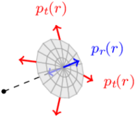
Figure 1: The radial pressure $p_{r}(r)$ and the tangential pressure $p_{t}(r)$ at a distance $r$ from the center of the system (31). Spherical symmetry imposes only the equality of the two tangential pressures.

We observe that the unpolarized static EMT in the BF (29) has the same structure as the EMT of an anisotropic spherically symmetric compact star Bayin:1985cd

$$\Theta^{\mu\nu}(\boldsymbol{r})=[\varepsilon(r)+p_{t}(r)]\,u^{\mu}u^{\nu}-p_{t}(r)\eta^{\mu\nu}+[p_{r}(r)-p_{t}(r)]\,\chi^{\mu}\chi^{\nu},$$ (31)

where $u^{\mu}$ and $\chi^{\mu}=x^{\mu}/r$ are unit timelike and spacelike four-vectors orthogonal to each other. The functions $\varepsilon(r)$, $p_{r}(r)$ and $p_{t}(r)$ represent the energy density, radial pressure and tangential pressure, respectively. As noticed by Einstein and developed first by Lemaitre in 1933 Lemaitre:1933gd2 ; Lemaitre:1933gd , spherical symmetry requires only the equality of the two tangential pressures, see Fig 1. The tensor (31) can alternatively be written as

$$\Theta^{\mu\nu}(\boldsymbol{r})=[\varepsilon(r)+p(r)]\,u^{\mu}u^{\nu}-p(r)\eta^{\mu\nu}+s(r)\left(\chi^{\mu}\chi^{\nu}-\frac{1}{3}\,h^{\mu\nu}\right)$$ (32)

with $h^{\mu\nu}=u^{\mu}u^{\nu}-\eta^{\mu\nu}$. Isotropic pressure $p(r)$ and pressure anisotropy $s(r)$ are related to radial and tangential pressures as follows

$$p(r)=\frac{p_{r}(r)+2\,p_{t}(r)}{3}\,,\qquad s(r)=p_{r}(r)-p_{t}(r)\,.$$ (33)

The comparison of the unpolarized static EMT in the BF (29) with the EMT of an anisotropic spherically symmetric compact star (31) or (32) with $u^{\mu}=\eta^{\mu 0}$ suggests that the following combinations

$$\varepsilon_{a}(r) =M\left\{\mathcal{A}_{a}(r)+\bar{\mathcal{C}}_{a}(r)+\frac{1}{4M^{2}}\frac{1}{r^{2}}\frac{\mathrm{d}}{\mathrm{d}r}\!\left(r^{2}\frac{\mathrm{d}}{\mathrm{d}r}\!\left[\mathcal{B}_{a}(r)-4\mathcal{C}_{a}(r)\right]\right)\right\},$$ (34)

$$p_{r,a}(r) =M\left\{-\bar{\mathcal{C}}_{a}(r)+\frac{1}{M^{2}}\frac{2}{r}\frac{\mathrm{d}\mathcal{C}_{a}(r)}{\mathrm{d}r}\right\},$$ (35)

$$p_{t,a}(r) =M\left\{-\bar{\mathcal{C}}_{a}(r)+\frac{1}{M^{2}}\frac{1}{r}\frac{\mathrm{d}}{\mathrm{d}r}\!\left(r\,\frac{\mathrm{d}\mathcal{C}_{a}(r)}{\mathrm{d}r}\right)\right\},$$ (36)

$$p_{a}(r) =M\left\{-\bar{\mathcal{C}}_{a}(r)+\frac{2}{3}\frac{1}{M^{2}}\frac{1}{r^{2}}\frac{\mathrm{d}}{\mathrm{d}r}\!\left(r^{2}\frac{\mathrm{d}\mathcal{C}_{a}(r)}{\mathrm{d}r}\right)\right\},$$ (37)

$$s_{a}(r) =M\left\{-\frac{1}{M^{2}}\,r\,\frac{\mathrm{d}}{\mathrm{d}r}\!\left(\frac{1}{r}\frac{\mathrm{d}\mathcal{C}_{a}(r)}{\mathrm{d}r}\right)\right\},$$ (38)

can be interpreted as the partial energy density, radial pressure, tangential pressure, isotropic pressure, and pressure anisotropy associated with constituent type $a$, respectively. They can alternatively be written as

$$\varepsilon_{a}(r) =M\int\frac{\mathrm{d}^{3}\boldsymbol{\Delta}}{(2\pi)^{3}}\,e^{-i\boldsymbol{\Delta}\cdot\boldsymbol{r}}\left\{A_{a}(t)+\bar{C}_{a}(t)+\frac{t}{4M^{2}}\left[B_{a}(t)-4C_{a}(t)\right]\right\},$$ (39)

$$p_{r,a}(r) =M\int\frac{\mathrm{d}^{3}\boldsymbol{\Delta}}{(2\pi)^{3}}\,e^{-i\boldsymbol{\Delta}\cdot\boldsymbol{r}}\left\{-\bar{C}_{a}(t)-\frac{4}{r^{2}}\frac{t^{-1/2}}{M^{2}}\frac{\mathrm{d}}{\mathrm{d}t}\!\left(t^{3/2}\,C_{a}(t)\right)\right\},$$ (40)

$$p_{t,a}(r) =M\int\frac{\mathrm{d}^{3}\boldsymbol{\Delta}}{(2\pi)^{3}}\,e^{-i\boldsymbol{\Delta}\cdot\boldsymbol{r}}\left\{-\bar{C}_{a}(t)+\frac{4}{r^{2}}\frac{t^{-1/2}}{M^{2}}\frac{\mathrm{d}}{\mathrm{d}t}\!\left[t\frac{\mathrm{d}}{\mathrm{d}t}\!\left(t^{3/2}\,C_{a}(t)\right)\right]\right\},$$ (41)

$$p_{a}(r) =M\int\frac{\mathrm{d}^{3}\boldsymbol{\Delta}}{(2\pi)^{3}}\,e^{-i\boldsymbol{\Delta}\cdot\boldsymbol{r}}\left\{-\bar{C}_{a}(t)+\frac{2}{3}\frac{t}{M^{2}}\,C_{a}(t)\right\},$$ (42)

$$s_{a}(r) =M\int\frac{\mathrm{d}^{3}\boldsymbol{\Delta}}{(2\pi)^{3}}\,e^{-i\boldsymbol{\Delta}\cdot\boldsymbol{r}}\left\{-\frac{4}{r^{2}}\frac{t^{-1/2}}{M^{2}}\frac{\mathrm{d}^{2}}{\mathrm{d}t^{2}}\!\left(t^{5/2}\,C_{a}(t)\right)\right\},$$ (43)

As indicated by the presence of $B_{a}(t)$, the non-zero spin of the target affects only the energy distribution in the BF. Classically, we indeed expect angular momentum to push matter away from the center.

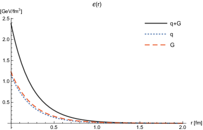
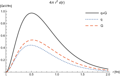
(a)                                                           (b)

Figure 2: Plots of the energy density, (a) $\epsilon(r)$ and (b) $4\pi\,r^{2}\,\epsilon(r)$, using the multipole model (11) with parameters given in Table 1, see Eq. (34) or Eq. (39) for the definition in terms of GFFs.

The above distributions are illustrated in Figs. 2-7 in units of GeV/fm${}^{3}=1.7827\times 10^{15}$ g/cm³ using the multipole model (11) with parameters given in Table 1. The energy density in Fig. 2 is always positive and is approximately shared equally between quark and gluon contributions. One defines the corresponding average squared mass radius as

$$R^{2}_{M}=\frac{1}{M}\int\mathrm{d}^{3}\boldsymbol{r}\,r^{2}\,\varepsilon(r)=6\left[\frac{\mathrm{d}A(t)}{\mathrm{d}t}\Big{|}_{t=0}-\frac{1}{M^{2}}\,C(0)\right].$$ (44)

In our simple model, we find $R_{M}=0\,.905$ fm which is a bit larger than the charge radius $R_{Q}=0\,.841$ fm extracted from muonic hydrogen spectroscopy Pohl:2010zza ; Pohl1:2016xoo and $R_{Q}=0\,.879$ fm extracted from electron-proton scattering Arrington:2015yxa . Knowing the distribution of energy density, it is also easy to derive the standard mass function widely used in General Relativity

$$m(r)=4\pi\int_{0}^{r}\mathrm{d}r^{\prime}\,r^{\prime 2}\,\varepsilon(r^{\prime})$$ (45)

which represents the mass contained within a sphere of radius $r$, see Fig. 3.

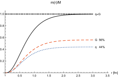
Figure 3: Quark, gluon and total mass functions, computed using the multipole model (11) with parameters given in Table 1, see Eq. (45) for the definition.

While the total radial pressure in Fig. 4 is always positive and largely dominated by the quark contribution, the total tangential and isotropic pressures in Figs. 5 and 6 switch from positive sign at the center of the nucleon (where it is dominated by the quark contribution) to negative sign at the periphery (where it is dominated by the gluon contribution). The pressure anisotropy in Fig. 7 vanishes at the center of the nucleon, as required by spherical symmetry, and is positive anywhere else, indicating that the radial pressure is always larger than the tangential one. Looking at the separate contributions, we see that the quark and gluon radial forces are both repulsive and of similar range. For the tangential forces, the quark contribution appears to be mostly repulsive and short range whereas the gluon contribution appears to be mostly attractive and long range.

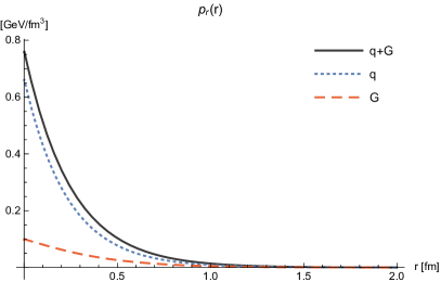
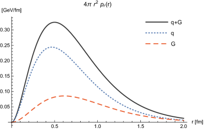
(a)                                                           (b)

Figure 4: Plots of the radial pressure, (a) $p_{r}(r)$ and (b) $4\pi\,r^{2}\,p_{r}(r)$, using the multipole model (11) with parameters given in Table 1, see Eq. (35) or Eq. (40) for definitions in terms of GFFs.

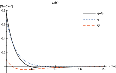
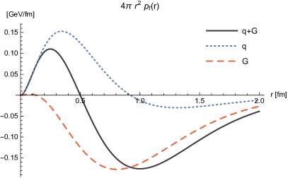
(a)                                                           (b)

Figure 5: Plots of the tangential pressure, (a) $p_{t}(r)$ and (b) $4\pi\,r^{2}\,p_{t}(r)$, using the multipole model (11) with parameters given in Table 1, see Eq. (36) or Eq. (41) for definitions in terms of GFFs.

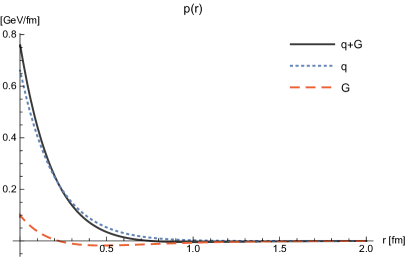
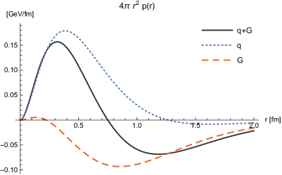
(a)                                                           (b)

Figure 6: Plots of the isotropic pressure, (a) $p(r)$ and (b) $4\pi\,r^{2}\,p(r)$, using the multipole model (11) with parameters given in Table 1, see Eq. (37) or Eq. (42) for definitions in terms of GFFs.

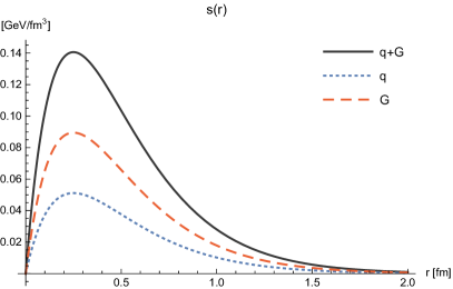
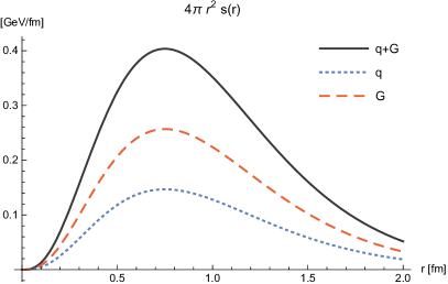
(a)                                                           (b)

Figure 7: Plots of the pressure anisotropy, (a) $s(r)$ and (b) $4\pi\,r^{2}\,s(r)$, using the multipole model (11) with parameters given in Table 1, see Eq. (38) or Eq. (43) for definitions in terms of GFFs.

If we integrate the energy density and the isotropic pressure over the whole volume, we naturally recover the FL (26) discussed in the former section

$$\int\mathrm{d}^{3}\boldsymbol{r}\,\varepsilon_{a}(r)=\left[A_{a}(0)+\bar{C}_{a}(0)\right]M,\qquad\int\mathrm{d}^{3}\boldsymbol{r}\,p_{a}(r)=-\bar{C}_{a}(0)\,M.$$ (46)

One can also relate the value of the GFF $C_{a}(t)$ at $t=0$ to a weighted integral of the pressure anisotropy (43) Polyakov:2002yz ; Goeke:2007fp ; Polyakov:2018zvc

$$\int\mathrm{d}^{3}\boldsymbol{r}\,r^{2}\,s_{a}(r)=-\frac{15}{M}\,C_{a}(0)\,.$$ (47)

Summing over the constituents, one obtains the following additional relations Goeke:2007fp ; Perevalova:2016dln

$$\int\mathrm{d}^{3}\boldsymbol{r}\,r^{2}p_{r}(r)=-\frac{6}{M}\,C(0)\,,\qquad\int\mathrm{d}^{3}\boldsymbol{r}\,r^{2}p_{t}(r)=\frac{9}{M}\,C(0)\,,\qquad\int\mathrm{d}^{3}\boldsymbol{r}\,r^{2}p(r)=\frac{4}{M}\,C(0)\,.$$ (48)

Several hints suggest that $C(0)$ is likely negative Goeke:2007fp ; Hudson:2017xug ; Hudson:2017oul ; Polyakov:2018zvc . Hudson and Schweitzer Hudson:2017xug observed that while adding total derivatives to the EMT leaves the Poincaré generators unaffected (and hence the particle mass and spin), it does change $C(0)$. Since this term can be extracted from experimental data, one should not be allowed to add these divergence terms without changing some scheme prescriptions, contrary to the common belief. The same conclusion is reached when one consistently treats intrinsic angular momentum at the level of spatial distributions Lorce:2017wkb ; Lorce:2018zpf .

Interestingly, in view of the energy density and pressure conditions encountered in a nucleon, one may conjecture that studies of the nucleon EMT will shed some light on the EoS inside compact stars Lorce:2017xzd , which so far remains largely unknown Ozel:2016oaf , and will therefore complement efforts based on heavy-ion collisions Danielewicz:2002pu and gravitational wave observations Rezzolla:2016nxn ; Annala:2017llu ; Paschalidis:2017qmb ; Most:2018hfd ; Nandi:2018ami ; Urbano:2018nrs . Eliminating the radial variable $r$ in Eqs. (34)-(37), we obtain the nucleon EoS for radial pressure $p_{r}(\varepsilon)$, tangential pressure $p_{t}(\varepsilon)$, and isotropic pressure $p(\varepsilon)$. The results plotted in Figs. 8 and 9 show a pretty stiff behavior compatible with the observation of supermassive ($\sim 2\,M_{\odot}$) compact stars Demorest:2010bx ; Antoniadis:2013pzd ; Annala:2017llu well above the Chandrasekhar mass limit $1.44\,M_{\odot}$ Chandrasekhar:1931ih . Although our multipole model is very naive, it supports the idea of an exciting crosstalk between hadronic physics and compact stars. An example of such a connection is given by the use of hadronic models to study the EoS of potential quark matter inside compact stars Baym:1976yu ; Haensel:1986qb ; Alcock:1986hz ; Drago:1995ah ; RikovskaStone:2006ta ; Stone:2010jt ; Motta:2018rxp ; Deb:2018 ; Abhishek:2018xml ; Jokela:2018ers .

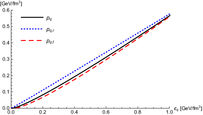
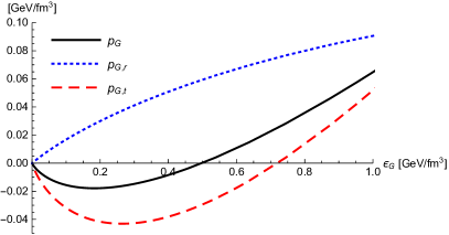
(a)                                                           (b)

Figure 8: Radial $p_{r}(\varepsilon)$, tangential $p_{t}(\varepsilon)$, and isotropic $p(\varepsilon)$ EoS for (a) quarks and (b) gluons computed using the multipole model (11) with parameters given in Table 1, see Eqs. (34)-(37) for definitions.

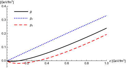
Figure 9: Radial $p_{r}(\varepsilon)$, tangential $p_{t}(\varepsilon)$, and isotropic $p(\varepsilon)$ EoS of the nucleon computed using the multipole model (11) with parameters given in Table 1, see Eqs. (34)-(37) for definitions.

III.3 Elastic frame

Spatial distributions with quasi-probabilistic interpretation can also be introduced when $\boldsymbol{P}\neq\boldsymbol{0}$ Lorce:2017wkb . In order to maintain the condition $\Delta^{0}=0$, we have to restrict ourselves to the set of elastic frames (EF) defined by $\boldsymbol{P}\cdot\boldsymbol{\Delta}=0$. They can be obtained by integrating the static EMT over the longitudinal coordinate $r^{\parallel}=\boldsymbol{r}\cdot\boldsymbol{P}/|\boldsymbol{P}|$

$$\mathsf{T}^{\mu\nu}_{a}(\boldsymbol{b}_{\perp};\boldsymbol{P})=\int\mathrm{d}r^{\parallel}\,\mathcal{T}^{\mu\nu}_{a}(\boldsymbol{r};\boldsymbol{P})=\int\frac{\mathrm{d}^{2}\boldsymbol{\Delta}_{\perp}}{(2\pi)^{2}}\,e^{-i\boldsymbol{\Delta}_{\perp}\cdot\boldsymbol{b}_{\perp}}\,\langle\!\langle T^{\mu\nu}_{a}(0)\rangle\!\rangle\big{|}_{\text{EF}},$$ (49)

where $\boldsymbol{\Delta}_{\perp}$ and $\boldsymbol{b}_{\perp}=\boldsymbol{r}_{\perp}$ are vectors lying in the two-dimensional plane orthogonal to $\boldsymbol{P}$, see Fig. 10.

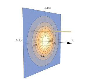
Figure 10: Density plot of the two-dimensional energy density $\rho(\boldsymbol{b}_{\perp})$ using the multipole model (11) with parameters given in Table 1, see Eq. (56) or Eq. (61) for the definition in terms of GFFs. The cylinder parallel to $\boldsymbol{P}=P_{z}\,\boldsymbol{e}_{z}$ illustrates the integration over $r^{\parallel}$, see Eq. (49).

The unpolarized off-forward amplitude (18) in the EF takes the form

$$\langle\!\langle T^{\mu\nu}_{a}(0)\rangle\!\rangle\big{|}_{\text{EF}} =\left[1-\frac{\boldsymbol{P}^{2}}{P^{0}(P^{0}+M)}\right]\!\left\{\frac{P^{\mu}P^{\nu}}{M}\,A_{a}(t)+\frac{\Delta^{\mu}_{\perp}\Delta^{\nu}_{\perp}+\eta^{\mu\nu}\boldsymbol{\Delta}^{2}_{\perp}}{M}\,C_{a}(t)+M\eta^{\mu\nu}\bar{C}_{a}(t)\right\}$$ (50)

$$-\frac{\boldsymbol{\Delta}^{2}_{\perp}}{4P^{0}(P^{0}+M)}\left\{\left[\frac{2P^{\mu}P^{\nu}}{M}+P^{\{\mu}\eta^{\nu\}0}\right]\frac{A_{a}(t)+B_{a}(t)}{2}+P^{[\mu}\eta^{\nu]0}\,\frac{D_{a}(t)}{2}\right\}\,,$$

where $P^{0}=\sqrt{\boldsymbol{P}^{2}+\frac{\boldsymbol{\Delta}^{2}_{\perp}}{4}+M^{2}}$ and $\Delta^{0}_{\perp}=\Delta^{\parallel}_{\perp}=0$. If we further integrate the static EMT over the impact-parameter $\boldsymbol{b}_{\perp}$, which amounts to setting $\boldsymbol{\Delta}_{\perp}=\boldsymbol{0}_{\perp}$ in Eq. (50), we recover the FL expression (22). If we set $\boldsymbol{P}=\boldsymbol{0}$ in Eq. (50), we recover the BF expression (28) integrated over $r^{\parallel}$, i.e. with $\Delta^{\parallel}=0$.

Since $P^{0}$ depends on $\boldsymbol{\Delta}_{\perp}$ in the EF, we could not find simple expressions for the spatial distributions $\mathsf{T}^{\mu\nu}_{a}(\boldsymbol{b}_{\perp};\boldsymbol{P})$ in terms of Fourier transforms of GFFs. Moreover, these spatial distributions will be $|\boldsymbol{P}|$-dependent. Let us choose for convenience the $z$-axis along $\boldsymbol{P}$. If we restrict ourselves to the (1+2)-dimensional (or transverse) static EMT with components $\alpha,\beta\in\{0,1,2\}$, its structure looks the same as that of an anisotropic axially symmetric compact star in two dimensions

$$t^{\alpha\beta}(\boldsymbol{b}_{\perp};P_{z})=[\gamma^{2}\rho(b,P_{z})+\sigma_{t}(b,P_{z})]\,v^{\alpha}v^{\beta}-\sigma_{t}(b,P_{z})\eta^{\alpha\beta}+[\sigma_{r}(b,P_{z})-\sigma_{t}(b,P_{z})]\,\chi^{\alpha}\chi^{\beta}\,,$$ (51)

where $v^{\alpha}=(1,\boldsymbol{0}_{\perp})$ and $\chi^{\alpha}=(0\,,\boldsymbol{b}_{\perp}/b)$. The functions $\rho(b,P_{z})$, $\sigma_{r}(b,P_{z})$ and $\sigma_{t}(b,P_{z})$ represent the two-dimensional version of energy density, radial pressure and tangential pressure, respectively. Note that we have included explicitly a factor of $\gamma^{2}$ in the energy density component that comes from the longitudinal Lorentz boost $t^{00}(\boldsymbol{b}_{\perp};P_{z})=\rho(b,P_{z})\,u^{0}u^{0}=\gamma^{2}\rho(b,P_{z})\,v^{0}v^{0}$, allowing us to compare directly $\rho(b,P_{z})$ for different values of $P_{z}$. In particular, for the total EMT we have $\int\mathrm{d}^{2}b_{\perp}\,\rho(b,P_{z})=M$. The tensor $t^{\alpha\beta}$ can alternatively be written as

$$t^{\alpha\beta}(\boldsymbol{b}_{\perp};P_{z})=[\gamma^{2}\rho(b,P_{z})+\sigma(b,P_{z})]\,v^{\alpha}v^{\beta}-\sigma(b,P_{z})\eta^{\alpha\beta}+\Pi(b,P_{z})\left(\chi^{\alpha}\chi^{\beta}-\frac{1}{2}\,l^{\alpha\beta}\right)$$ (52)

with $l^{\alpha\beta}=v^{\alpha}v^{\beta}-\eta^{\alpha\beta}$. The two-dimensional isotropic pressure $\sigma(b,P_{z})$ and pressure anisotropy $\Pi(b,P_{z})$ are related to radial and tangential pressures as follows

$$\sigma(b,P_{z})=\frac{\sigma_{r}(b,P_{z})+\sigma_{t}(b,P_{z})}{2}\,,\qquad\Pi(b,P_{z})=\sigma_{r}(b,P_{z})-\sigma_{t}(b,P_{z})\,.$$ (53)

The particular case $P_{z}=0$ is simple and corresponds to the BF. We find

$$\mathsf{T}^{\alpha\beta}_{a}(\boldsymbol{b}_{\perp};\boldsymbol{0})=M \left\{\eta^{\alpha 0}\eta^{\beta 0}\left[\mathsf{A}_{a}(b)+\frac{1}{4M^{2}}\frac{1}{b}\frac{\mathrm{d}}{\mathrm{d}b}\!\left(b\,\frac{\mathrm{d}\mathsf{B}_{a}(b)}{\mathrm{d}b}-4\mathsf{C}_{a}(b)\right)\right]\right.$$ (54)

$$\left.+\eta^{\alpha\beta}\left[\bar{\mathsf{C}}_{a}(b)-\frac{1}{M^{2}}\frac{\mathrm{d}^{2}\mathsf{C}_{a}(b)}{\mathrm{d}b^{2}}\right]-\frac{x^{\alpha}x^{\beta}}{b^{2}}\,\frac{1}{M^{2}}\,b\,\frac{\mathrm{d}}{\mathrm{d}b}\!\left(\frac{1}{b}\frac{\mathrm{d}\mathsf{C}_{a}(b)}{\mathrm{d}b}\right)\right\}\,,$$

where $x^{\alpha}=(0,\boldsymbol{b}_{\perp})$ and the two-dimensional Fourier transforms of GFFs are denoted by

$$\mathsf{F}_{a}(b)=\int\frac{\mathrm{d}^{2}\boldsymbol{\Delta}_{\perp}}{(2\pi)^{2}}\,e^{-i\boldsymbol{\Delta}_{\perp}\cdot\boldsymbol{b}_{\perp}}\,F_{a}(t)$$ (55)

with $t=-\boldsymbol{\Delta}^{2}_{\perp}$. Comparing Eq. (54) with the EMT of an anisotropic axially symmetric compact star in two dimensions (51) and (52) suggests that the following combinations

$$\rho_{a}(b,0) =M\left\{\mathsf{A}_{a}(b)+\bar{\mathsf{C}}_{a}(b)+\frac{1}{4M^{2}}\frac{1}{b}\frac{\mathrm{d}}{\mathrm{d}b}\!\left(b\,\frac{\mathrm{d}}{\mathrm{d}b}\!\left[\mathsf{B}_{a}(b)-4\mathsf{C}_{a}(b)\right]\right)\right\},$$ (56)

$$\sigma_{r,a}(b,0) =M\left\{-\bar{\mathsf{C}}_{a}(b)+\frac{1}{M^{2}}\frac{1}{b}\frac{\mathrm{d}\mathsf{C}_{a}(b)}{\mathrm{d}b}\right\},$$ (57)

$$\sigma_{t,a}(b,0) =M\left\{-\bar{\mathsf{C}}_{a}(b)+\frac{1}{M^{2}}\frac{\mathrm{d}^{2}\mathsf{C}_{a}(b)}{\mathrm{d}b^{2}}\right\},$$ (58)

$$\sigma_{a}(b,0) =M\left\{-\bar{\mathsf{C}}_{a}(b)+\frac{1}{2M^{2}}\frac{1}{b}\frac{\mathrm{d}}{\mathrm{d}b}\!\left(b\,\frac{\mathrm{d}\mathsf{C}_{a}(b)}{\mathrm{d}b}\right)\right\},$$ (59)

$$\Pi_{a}(b,0) =M\left\{-\frac{1}{M^{2}}\,b\,\frac{\mathrm{d}}{\mathrm{d}b}\!\left(\frac{1}{b}\frac{\mathrm{d}\mathsf{C}_{a}(b)}{\mathrm{d}b}\right)\right\},$$ (60)

can be interpreted as the two-dimensional partial energy density, radial pressure, tangential pressure, isotropic pressure, and pressure anisotropy associated with constituent type $a$. They can alternatively be written as

$$\rho_{a}(b,0) =M\int\frac{\mathrm{d}^{2}\boldsymbol{\Delta}_{\perp}}{(2\pi)^{2}}\,e^{-i\boldsymbol{\Delta}_{\perp}\cdot\boldsymbol{b}_{\perp}}\left\{A_{a}(t)+\bar{C}_{a}(t)+\frac{t}{4M^{2}}\left[B_{a}(t)-4C_{a}(t)\right]\right\}\,,$$ (61)

$$\sigma_{r,a}(b,0) =M\int\frac{\mathrm{d}^{2}\boldsymbol{\Delta}_{\perp}}{(2\pi)^{2}}\,e^{-i\boldsymbol{\Delta}_{\perp}\cdot\boldsymbol{b}_{\perp}}\left\{-\bar{C}_{a}(t)-\frac{2}{b^{2}}\frac{1}{M^{2}}\frac{\mathrm{d}}{\mathrm{d}t}\!\left[t\,C_{a}(t)\right]\right\}\,,$$ (62)

$$\sigma_{t,a}(b,0) =M\int\frac{\mathrm{d}^{2}\boldsymbol{\Delta}_{\perp}}{(2\pi)^{2}}\,e^{-i\boldsymbol{\Delta}_{\perp}\cdot\boldsymbol{b}_{\perp}}\left\{-\bar{C}_{a}(t)+\frac{1}{b^{2}}\frac{4}{M^{2}}\frac{\mathrm{d}}{\mathrm{d}t}\!\left[t^{1/2}\frac{\mathrm{d}}{\mathrm{d}t}\!\left(t^{3/2}\,C_{a}(t)\right)\right]\right\}\,,$$ (63)

$$\sigma_{a}(b,0) =M\int\frac{\mathrm{d}^{2}\boldsymbol{\Delta}_{\perp}}{(2\pi)^{2}}\,e^{-i\boldsymbol{\Delta}_{\perp}\cdot\boldsymbol{b}_{\perp}}\left\{-\bar{C}_{a}(t)+\frac{1}{2}\frac{t}{M^{2}}\,C_{a}(t)\right\}\,,$$ (64)

$$\Pi_{a}(b,0) =M\int\frac{\mathrm{d}^{2}\boldsymbol{\Delta}_{\perp}}{(2\pi)^{2}}\,e^{-i\boldsymbol{\Delta}_{\perp}\cdot\boldsymbol{b}_{\perp}}\left\{-\frac{1}{b^{2}}\frac{4}{M^{2}}\frac{\mathrm{d}^{2}}{\mathrm{d}t^{2}}\!\left[t^{2}C_{a}(t)\right]\right\}\,.$$ (65)

Integrating Eq. (29) over $z$ allows us to alternatively express these quantities in terms of the three-dimensional energy density and pressures as follows

$$\rho_{a}(b,0) =\int\mathrm{d}z\,\varepsilon_{a}(r)\,,$$ (66)

$$\sigma_{r,a}(b,0) =\int\mathrm{d}z\,\frac{b^{2}p_{r,a}(r)+z^{2}p_{t,a}(r)}{r^{2}}\,,$$ (67)

$$\sigma_{t,a}(b,0) =\int\mathrm{d}z\,p_{t,a}(r)\,,$$ (68)

$$\sigma_{a}(b,0) =\int\mathrm{d}z\left[p_{a}(r)+\frac{b^{2}-2z^{2}}{6r^{2}}\,s_{a}(r)\right],$$ (69)

$$\Pi_{a}(b,0) =\int\mathrm{d}z\,\frac{b^{2}}{r^{2}}\,s_{a}(r)\,,$$ (70)

with $r=\sqrt{b^{2}+z^{2}}$.

These distributions are illustrated in Figs. 11–15 in units of GeV/fm${}^{2}=178.27$ g/cm² using the multipole model (11) with parameters given in Table 1. Their behavior turns out to be similar to the corresponding three-dimensional distributions, see Figs. 2-7, except for the gluon contribution to the radial pressure, compare Figs. 4 and 12. This is an effect of the projection onto the transverse plane which mixes three-dimensional radial and tangential pressures together, as indicated by Eq. (67). While the latter have the same sign for quarks, they are of opposite sign for gluons.

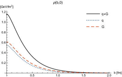
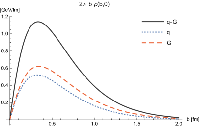
(a)                                                           (b)

Figure 11: Plots of the two-dimensional energy density, (a) $\rho(b,0)$ and (b) $2\pi\,b\,\rho(b,0)$, using the multipole model (11) with parameters given in Table 1, see Eq. (56) or Eq. (61) for the definition in terms of GFFs.

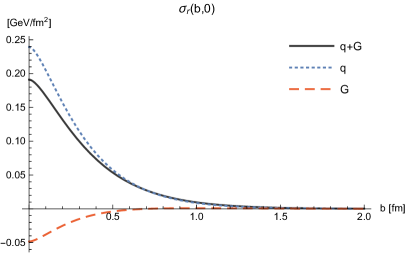
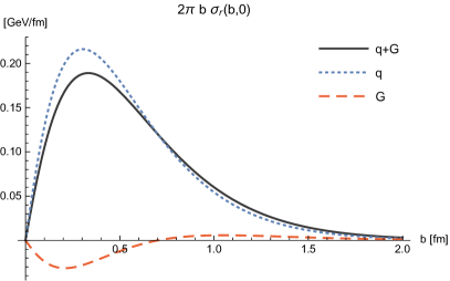
(a)                                                           (b)

Figure 12: Plots of the two-dimensional radial pressure, (a) $\sigma_{r}(b,0)$ and (b) $2\pi\,b\,\sigma_{r}(b,0)$, using the multipole model (11) with parameters given in Table 1, see Eq. (57) or Eq. (62) for the definition in terms of GFFs.

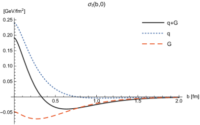
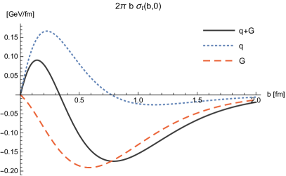
(a)                                                           (b)

Figure 13: Plots of the two-dimensional tangential pressure, (a) $\sigma_{t}(b,0)$ and (b) $2\pi\,b\,\sigma_{t}(b,0)$, using the multipole model (11) with parameters given in Table 1, see Eq. (58) or (63) for the definition in terms of GFFs.

(a)                                                           (b)

Figure 14: Plots of the two-dimensional isotropic pressure, (a) $\sigma(b,0)$ and (b) $2\pi\,b\,\sigma(b,0)$, using the multipole model (11) with parameters given in Table 1, see Eq. (59) or (64) for the definition in terms of GFFs.

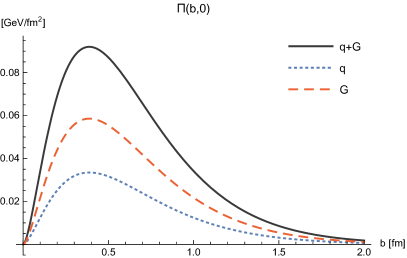
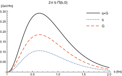
(a)                                                           (b)

Figure 15: Plots of the two-dimensional pressure anisotropy, (a) $\Pi(b,0)$ and (b) $2\pi\,b\,\Pi(b,0)$, using the multipole model (11) with parameters given in Table 1, see Eq. (60) or (65) for the definition in terms of GFFs.

Similarly to the three-dimensional case, we can relate the value of the GFF $C_{a}(t)$ at $t=0$ to a weighted integral of the pressure anisotropy

$$\int\mathrm{d}^{2}\boldsymbol{b}_{\perp}\,b^{2}\,\Pi_{a}(b,0)=-\frac{8}{M}\,C_{a}(0)\,.$$ (71)

Summing over the constituents, we also find the additional relations

$$\int\mathrm{d}^{2}\boldsymbol{b}_{\perp}\,b^{2}\sigma_{r}(b,0)=-\frac{2}{M}\,C(0)\,,\qquad\int\mathrm{d}^{2}\boldsymbol{b}_{\perp}\,b^{2}\sigma_{t}(b,0)=\frac{6}{M}\,C(0)\,,\qquad\int\mathrm{d}^{2}\boldsymbol{b}_{\perp}\,b^{2}\sigma(b,0)=\frac{2}{M}\,C(0)\,,$$ (72)

which are simply the two-dimensional version of those appearing in Eq. (48).

The last term in Eq. (50) makes the EMT asymmetric. In particular, the density of longitudinal momentum $\mathcal{T}^{03}_{a}$ is not equal to the longitudinal flux of energy $\mathcal{T}^{30}_{a}$ when the GFF $D_{a}(t)$ is not identically zero. Using Poincaré invariance, the antisymmetric part of the EMT $T^{[\mu\nu]}$ can be expressed in terms of the intrinsic angular momentum current $S^{\lambda\mu\nu}$ as follows Leader:2013jra ; Lorce:2017wkb

$$T^{[\mu\nu]}(x)=-\partial_{\lambda}S^{\lambda\mu\nu}(x)\,.$$ (73)

In the case of QCD, we get for the corresponding off-forward matrix elements

$$\langle\!\langle T^{[\mu\nu]}_{q}(0)\rangle\!\rangle=-\frac{i}{2}\,\epsilon^{\mu\nu\Delta\lambda}\,\langle\!\langle\overline{\psi}(0)\gamma_{\lambda}\gamma_{5}\psi(0)\rangle\!\rangle\,,$$ (74)

where the matrix elements of the axial-vector current are parametrized as follows

$${\left\langle p^{\prime},\boldsymbol{s}\right|}\overline{\psi}(0)\gamma^{\mu}\gamma_{5}\psi(0){\left|p,\boldsymbol{s}\right\rangle}=\bar{u}(p^{\prime},\boldsymbol{s})\left[\gamma^{\mu}\gamma_{5}\,G^{q}_{A}(t)+\frac{\Delta^{\mu}\gamma_{5}}{2M}\,G^{q}_{P}(t)\right]u(p,\boldsymbol{s})$$ (75)

in terms of the axial-vector and induced pseudoscalar form factors. According to Ref. Lorce:2017isp , the corresponding bilinears can be expressed in instant form as

$$\bar{u}^{\prime}\gamma_{5}u =\mathcal{N}^{-1}\left[(P^{0}+M)\,(\Delta\cdot S)-\Delta^{0}(P\cdot S)\right],$$ (76)

$$\bar{u}^{\prime}\gamma^{\mu}\gamma_{5}u =\mathcal{N}^{-1}\left\{2\left[S^{\mu}(P^{2}+P^{0}M)-(P^{\mu}+\eta^{\mu 0}M)\,(P\cdot S)+\frac{\Delta^{\mu}(\Delta\cdot S)}{4}\right]+i\epsilon^{\mu P\Delta 0}\right\}\,.$$ (77)

For an unpolarized target $S^{\mu}=0$, we can write

$$\langle\!\langle\overline{\psi}(0)\gamma^{\mu}\gamma_{5}\psi(0)\rangle\!\rangle=\frac{i\epsilon^{\mu P\Delta 0}}{2P^{0}\mathcal{N}}\,G_{A}^{q}(t)\,,$$ (78)

and hence we find in the EF

$$\langle\!\langle T^{[\mu\nu]}_{q}(0)\rangle\!\rangle\big{|}_{\text{EF}}=\frac{\boldsymbol{\Delta}^{2}_{\perp}}{4P^{0}(P^{0}+M)}\,P^{[\mu}\eta^{\nu]0}\,G^{q}_{A}(t)\,.$$ (79)

Using now the expression in Eq. (50) for the left-hand side, we recover the relation $D_{q}(t)=-G^{q}_{A}(t)$.

We are now ready to discuss the distribution of spin inside an unpolarized target. The quark spin operator being given by $\frac{1}{2}\,\overline{\psi}(0)\gamma^{i}\gamma_{5}\psi(0)$, the corresponding distribution in the EF is given by

$$\mathsf{S}^{i}(\boldsymbol{b}_{\perp};\boldsymbol{P})=-(\boldsymbol{P}\times\boldsymbol{\nabla})^{i}\int\frac{\mathrm{d}^{2}\boldsymbol{\Delta}_{\perp}}{(2\pi)^{2}}\,e^{-i\boldsymbol{\Delta}_{\perp}\cdot\boldsymbol{b}_{\perp}}\,\frac{G^{q}_{A}(t)}{4P^{0}(P^{0}+M)}.$$ (80)

We see that even in an unpolarized target, a nonzero quark spin distribution appears when the target is moving, see Fig. 16. The spin direction is orthogonal to both the target momentum and the impact parameter. This is reminiscent of transverse shifts observed for transversely polarized moving target, see Lorce:2018zpf and references therein. In the latter case, the transverse shifts appear because of a nonzero net orbital angular momentum in the system. In the present case, the appearance of transverse spin distribution is a result of spin-orbit coupling Lorce:2011kd ; Lorce:2014mxa ; Bhoonah:2017olu .

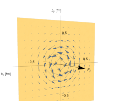
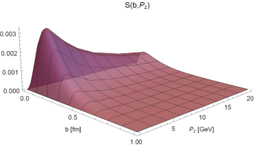
(a)                                                           (b)

Figure 16: Quark spin distribution $\boldsymbol{\mathsf{S}}(\boldsymbol{b}_{\perp};\boldsymbol{P})$ for $\boldsymbol{P}=(0\,,0\,,P_{z})$ using the multipole model (11) with parameters given in Table 1, see Eq. (80). (a) Distribution of the quark spin $\boldsymbol{\mathsf{S}}$ in impact-parameter space for $P_{z}$ = 0 .1 GeV, and (b) magnitude of the quark spin density $\mathsf{S}$ as a function of the impact-parameter $b$ and the target momentum $P_{z}$.

III.4 Infinite-momentum frame

The infinite-momentum frame (IMF) is a special case of the EF obtained by considering the limit $P_{z}\to\infty$ Weinberg:1966jm . We find that the (1+2)-dimensional unpolarized off-forward amplitude (50) reduces in the IMF to

$$\langle\!\langle T^{\alpha\beta}_{a}(0)\rangle\!\rangle\big{|}_{\text{IMF}} =\eta^{\alpha 0}\eta^{\beta 0}\left(E_{P}\,A_{a}(t)-\frac{\boldsymbol{\Delta}^{2}_{\perp}}{4M}\,B_{a}(t)-\frac{\boldsymbol{\Delta}^{2}_{\perp}}{8E_{P}}\,A_{a}(t)\right)$$ (81)

$$+\frac{M^{2}}{E_{P}}\left(\frac{\Delta^{\alpha}_{\perp}\Delta^{\beta}_{\perp}+\eta^{\alpha\beta}\boldsymbol{\Delta}^{2}_{\perp}}{M^{2}}\,C_{a}(t)+\eta^{\alpha\beta}\bar{C}_{a}(t)\right)+\mathcal{O}(P^{-2}_{z})\,.$$

After two-dimensional Fourier transform, we obtain for $\boldsymbol{P}_{\perp}=\boldsymbol{0}_{\perp}$

$$\mathsf{T}^{\alpha\beta}_{a}(\boldsymbol{b}_{\perp};\boldsymbol{0}_{\perp},P_{z})=\frac{M^{2}}{E_{P}} \left\{\eta^{\alpha 0}\eta^{\beta 0}\,\frac{E^{2}_{P}}{M^{2}}\left[\mathsf{A}_{a}(b)+\frac{1}{4E_{P}^{2}}\frac{1}{b}\frac{\mathrm{d}}{\mathrm{d}b}\!\left(b\,\frac{\mathrm{d}}{\mathrm{d}b}\!\left[\frac{E_{P}}{M}\,\mathsf{B}_{a}(b)+\frac{\mathsf{A}_{a}(b)}{2}\right]-4\mathsf{C}_{a}(b)\right)\right]\right.$$ (82)

$$\left.+\eta^{\alpha\beta}\left[\bar{\mathsf{C}}_{a}(b)-\frac{1}{M^{2}}\frac{\mathrm{d}^{2}\mathsf{C}_{a}(b)}{\mathrm{d}b^{2}}\right]-\frac{x^{\alpha}\,x^{\beta}}{b^{2}}\,\frac{1}{M^{2}}\,b\,\frac{\mathrm{d}}{\mathrm{d}b}\!\left(\frac{1}{b}\frac{\mathrm{d}\mathsf{C}_{a}(b)}{\mathrm{d}b}\right)\right\}+\mathcal{O}(P^{-2}_{z})\,,$$

where $x^{\alpha}=(0,\boldsymbol{b}_{\perp})$ and therefore, by comparison with Eqs. (51) and (52), we can write

$$\rho_{a}(b,P_{z}) \approx M\,\mathsf{A}_{a}(b),$$ (83)

$$\sigma_{r,a}(b,P_{z}) \approx M\left\{-\bar{\mathsf{C}}_{a}(b)+\frac{1}{M^{2}}\frac{1}{b}\frac{\mathrm{d}\mathsf{C}_{a}(b)}{\mathrm{d}b}\right\},$$ (84)

$$\sigma_{t,a}(b,P_{z}) \approx M\left\{-\bar{\mathsf{C}}_{a}(b)+\frac{1}{M^{2}}\frac{\mathrm{d}^{2}\mathsf{C}_{a}(b)}{\mathrm{d}b^{2}}\right\},$$ (85)

$$\sigma_{a}(b,P_{z}) \approx M\left\{-\bar{\mathsf{C}}_{a}(b)+\frac{1}{2}\frac{1}{M^{2}}\frac{1}{b}\frac{\mathrm{d}}{\mathrm{d}b}\!\left(b\,\frac{\mathrm{d}\mathsf{C}_{a}(b)}{\mathrm{d}b}\right)\right\},$$ (86)

$$\Pi_{a}(b,P_{z}) \approx M\left\{-\frac{1}{M^{2}}\,b\,\frac{\mathrm{d}}{\mathrm{d}b}\!\left(\frac{1}{b}\frac{\mathrm{d}\mathsf{C}_{a}(b)}{\mathrm{d}b}\right)\right\},$$ (87)

keeping only the leading terms in $P_{z}^{2}\gg P^{2}$ and taking the boost factor $\gamma=E_{P}/M$ into account in the identification $t^{\alpha\beta}\sim\gamma\,\mathsf{T}^{\alpha\beta}$.

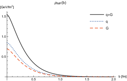
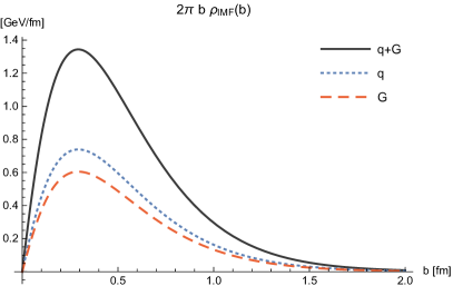
(a)                                                           (b)
  
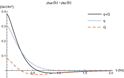
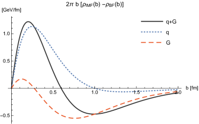
(c)                                                           (d)

Figure 17: Plots of the two-dimensional energy density in the IMF, (a) $\rho_{\text{IMF}}(b)=\lim_{P_{z}\to\infty}\rho(b,P_{z})$ and (b) $2\pi\,b\,\rho_{\text{IMF}}(b)$, and their difference with the corresponding densities in the BF (c) $\rho_{\text{IMF}}(b)-\rho_{\text{BF}}(b)$ with $\rho_{\text{BF}}=\rho(b,0)$ and (d) $2\pi\,b\,[\rho_{\text{IMF}}(b)-\rho_{\text{BF}}(b)]$, using the multipole model (11) with parameters given in Table 1, see Eqs. (56) or (61), and (83) for the definition in terms of GFFs.

While the two-dimensional pressures are the same in both the BF ($P_{z}=0$) and IMF ($P_{z}\to\infty$), the energy densities (56) and (83) differ. This may be interpreted by the expectation that kinetic energy grows with $P_{z}$ whereas binding energy associated with pressure forces remains constant. In the IMF, kinetic energy becomes by far the dominant contribution and we recover the parton picture where quarks and gluons behave as almost free massless particles. Since the two-dimensional pressures in the IMF coincides with those shown in Figs. 12-15, we simply illustrate in Fig. 17 the energy density in the IMF, using the multipole model (11) with parameters given in Table 1. The comparison with the energy density in the BF shows that the kinetic energy is more concentrated around the center of the nucleon than the binding energy. Naturally, once summed over all the constituents and integrated over the impact parameter space, the difference disappears.

IV Distributions in front form

The interpretation of form factors in the Breit frame are known to be plagued by relativistic corrections Burkardt:2000za ; Polyakov:2002yz ; Belitsky:2005qn . In particular, one could multiply the off-forward amplitude (18) by some function $f(P^{0}/E_{P})$ normalized as $f(1)=1$ to correct for Lorentz contractions effects. While such correction factor does not change the integrated quantities, it does change the spatial distributions since it introduces an additional $\boldsymbol{\Delta}$-dependence. Moreover, the correction factor cannot be determined in practice in a model-independent way because Lorentz boosts depend on the dynamics of the interacting system.

An interpretation free of such relativistic corrections can however be obtained using the light-front (LF) formalism Dirac:1949cp ; Brodsky:1997de , which amounts to adopting the point of view of a massless observer Lorce:2018zpf . This remarkable feature is explained by the fact that, in the LF formalism, the subgroup of Lorentz transformations associated with the transverse plane is Galilean Susskind:1967rg ; Burkardt:2002hr . Burkardt used this formalism and introduced the boost-invariant impact-parameter distributions (IPDs) of quarks and gluons Burkardt:2000za ; Burkardt:2002hr . Including parton transverse momentum to the picture led then to the concept of relativistic phase-space (or Wigner) distributions Lorce:2011kd ; Lorce:2011ni ; Lorce:2012ce ; Lorce:2015sqe . Longitudinal LF momentum IPDs Abidin:2008sb ; Selyugin:2009ic ; Son:2014sna ; Chakrabarti:2015lba ; Mondal:2015fok ; Mondal:2016xsm ; SattaryNikkhoo:2018odd ; Kumar:2017dbf ; Kumano:2017lhr ; Kaur:2018ewq and longitudinal angular momentum IPDs Adhikari:2016dir ; Lorce:2017wkb ; Kumar:2017dbf have also recently been discussed in the literature. Our aim here is to introduce the IPDs associated with the EMT.

IV.1 Light-front components

The LF components of a four-vector are given by

$$a^{\mu}=[a^{+},a^{-},\boldsymbol{a}_{\perp}]\,,$$ (88)

where $a^{\pm}=(a^{0}\pm a^{3})/\sqrt{2}$. In terms of these, the scalar product of two four-vectors reads

$$a\cdot b=a^{+}b^{-}+a^{-}b^{+}-\boldsymbol{a}_{\perp}\cdot\boldsymbol{b}_{\perp}.$$ (89)

One conventionally chooses $x^{+}$ to the represent the LF time coordinate. It then follows from Eq. (89) that $p^{-}$ represents the LF energy. The other conjugate components $x^{-}$ and $p^{+}$ represent the longitudinal LF coordinate and momentum, respectively. Without loss of generality, we choose the $z$-axis along $\boldsymbol{P}$, so that we simply have

$$P^{\mu}=[P^{+},P^{-},\boldsymbol{0}_{\perp}].$$ (90)

We will denote the spatial LF three-vectors as $\tilde{\boldsymbol{a}}$ and use a dotted notation to keep the tensor expressions compact. A LF three-vector with a dotted index will indicate a minus first component followed by the transverse ones, while an undotted index will indicate a plus first component followed by the transverse ones, i.e. $a^{\dot{\alpha}}=(a^{-},\boldsymbol{a}_{\perp})$ and $a^{\alpha}=(a^{+},\boldsymbol{a}_{\perp})$. Thus, in position space, the spatial LF coordinates read $x^{\dot{\alpha}}=(x^{-},\boldsymbol{x}_{\perp})$, and in momentum space they read $p^{\alpha}=(p^{+},\boldsymbol{p}_{\perp})$. We can then rewrite the scalar product of two four-vectors (89) as

$$x\cdot p=x^{+}p^{-}+\tilde{\boldsymbol{x}}\cdot\tilde{\boldsymbol{p}}$$ (91)

with $\tilde{\boldsymbol{x}}\cdot\tilde{\boldsymbol{p}}=x_{\dot{\alpha}}\,p^{\alpha}=x^{\dot{\alpha}}\,p_{\alpha}=x^{-}p^{+}-\boldsymbol{x}_{\perp}\cdot\boldsymbol{p}_{\perp}$. Using LF components is convenient because they behave in a simple way under LF boosts Dirac:1949cp ; Brodsky:1997de . In particular, performing a longitudinal LF boost amounts to a mere rescaling of the LF components $[a^{+},a^{-},\boldsymbol{a}_{\perp}]\mapsto[e^{-\omega}a^{+},e^{\omega}a^{-},\boldsymbol{a}_{\perp}]$, where $\gamma=\cosh\omega$.

Because of the Galilean symmetry in the transverse plane, it is interesting to organize the LF components of the EMT as follows Soper:1976bb

$$T^{\mu\nu}=\left(\begin{array}[]{ccc|c}T^{+-}&T^{+1}&T^{+2}&T^{++}\\ T^{1-}&T^{11}&T^{12}&T^{1+}\\ T^{2-}&T^{21}&T^{22}&T^{2+}\\ \hline\cr T^{--}&T^{-1}&T^{-2}&T^{-+}\end{array}\right).$$ (92)

The upper left corner corresponds to a (1+2)-dimensional Galilean EMT $T^{\alpha\dot{\beta}}$. The upper right corner corresponds to a “mass” current $J^{\alpha}=T^{\alpha+}$, where the role of “mass” in the transverse plane is played by the longitudinal LF momentum. Since we are considering only the static EMT, the above currents are conserved in the (1+2)-dimensional subspace

$$\partial_{\dot{\alpha}}T^{\alpha\dot{\beta}}=\partial_{-}T^{+\dot{\beta}}+\partial_{i}T^{i\dot{\beta}}=0\,,\qquad\partial_{\dot{\alpha}}J^{\alpha}=0\,.$$ (93)

Together, they form the so-called covariant non-relativistic stress-energy tensor $T^{\alpha\mu}$ appearing in the context of Newton-Cartan geometries, which find important applications in condensed matter and in the study of non-relativistic holographic systems, see e.g. Geracie:2016bkg and references therein. The last line in Eq. (92), which describes the flux of energy and momentum along the spatial LF direction $x^{-}$, does not have any known simple interpretation within the Galilean picture.

IV.2 Light-front amplitudes

We can repeat the same procedure as in Section III in the LF formalism. Integrating the covariant phase-space density operator (1) over $P^{2}$ and $\Delta^{-}$ leads to

$$\rho_{R,P}=\int\frac{\mathrm{d}^{3}\tilde{\boldsymbol{\Delta}}}{(2\pi)^{3}\,2P^{+}}\,e^{-i\Delta\cdot R}\,{\left|P-\tfrac{\Delta}{2}\right\rangle}{\left\langle P+\tfrac{\Delta}{2}\right|}\,,$$ (94)

with $\Delta^{-}=-\Delta^{+}\,P^{-}/P^{+}$, since $\boldsymbol{P}_{\perp}=\boldsymbol{0}_{\perp}$ (90), and

$$p^{-}=\frac{\frac{\boldsymbol{\Delta}_{\perp}^{2}}{4}+M^{2}}{2\left(P^{+}-\frac{\Delta^{+}}{2}\right)}\,,\qquad p^{\prime-}=\frac{\frac{\boldsymbol{\Delta}_{\perp}^{2}}{4}+M^{2}}{2\left(P^{+}+\frac{\Delta^{+}}{2}\right)}\,.$$ (95)

The non-explicitly covariant form (94) coincides with that in Ref. Lorce:2017wkb if we replace the normalization factor $2P^{+}$ by $2\sqrt{p^{\prime+}p^{+}}$. Once again, the difference in the normalization comes from the fact that “position” states in Ref. Lorce:2017wkb were defined with the non-relativistic normalization $\langle x^{\prime}|x\rangle=\delta^{(3)}(\tilde{\boldsymbol{x}}^{\prime}-\tilde{\boldsymbol{x}})$ at equal LF times. This difference will however not concern us since we will essentially be interested in the case $\Delta^{-}=p^{\prime-}-p^{-}=0$.

Setting the origin at the average position of the system, the LF distribution of energy and momentum inside the system with canonical polarization $\boldsymbol{s}$ and average LF momentum $\tilde{\boldsymbol{P}}=(P^{+},\boldsymbol{0}_{\perp})$ is given by the Fourier transform

$$\mathcal{T}^{\mu\nu}_{a}(\tilde{\boldsymbol{x}};\tilde{\boldsymbol{P}})=\langle T^{\mu\nu}_{a}(\tilde{\boldsymbol{x}})\rangle_{0,P}=\int\frac{\mathrm{d}^{3}\tilde{\boldsymbol{\Delta}}}{(2\pi)^{3}}\,e^{i\tilde{\boldsymbol{\Delta}}\cdot\tilde{\boldsymbol{x}}}\,\langle\!\langle T^{\mu\nu}_{a}(0)\rangle\!\rangle$$ (96)

of the LF off-forward amplitude Lorce:2017wkb

$$\langle\!\langle T^{\mu\nu}_{a}(0)\rangle\!\rangle=\frac{{\left\langle p^{\prime},\boldsymbol{s}\right|}T^{\mu\nu}_{a}(0){\left|p,\boldsymbol{s}\right\rangle}}{2P^{+}}\,.$$ (97)

Note that $x^{+}=0$ because the LF positions $\boldsymbol{X}^{-}$ and $\boldsymbol{R}^{-}$ are considered at the same LF time $X^{+}=R^{+}$. If we allow $X^{+}$ and $R^{+}$ to be different, the above static EMT $\mathcal{T}^{\mu\nu}_{a}(\tilde{\boldsymbol{x}};\tilde{\boldsymbol{P}})$ can be recovered by considering the LF time average $\int{\mathrm{d}X^{+}}/[2\pi\,\delta(0)]$ in a frame where the LF energy transfer vanishes $\Delta^{-}=0$.

The Dirac bilinears appearing in the parametrization of the EMT (8) can be expressed in front form as Lorce:2017isp

$$\bar{u}^{\prime}u =\mathcal{N}^{-1}\left[2MP^{+}+i\epsilon^{+P\Delta S_{\perp}}\right],$$ (98)

$$\bar{u}^{\prime}i\sigma^{\mu\Delta}u =\mathcal{N}^{-1}\left\{M(\eta^{\mu+}\Delta^{2}-\Delta^{\mu}\Delta^{+})+2\left[P^{+}\,i\epsilon^{\mu\Delta PS_{\perp}}-\frac{\Delta^{2}}{4}\,i\epsilon^{\mu\Delta S_{\perp}+}-\left[(P\cdot S_{\perp})+Ms_{z}\right]i\epsilon^{\mu\Delta P+}\right]\right\},$$ (99)

where $S^{\mu}_{\perp}=[0\,,0\,,\boldsymbol{s}_{\perp}]$ and $\mathcal{N}=\sqrt{p^{\prime+}}\sqrt{p^{+}}$. The unpolarized off-forward LF amplitude then reads

$$\langle\!\langle T^{\mu\nu}_{a}(0)\rangle\!\rangle =\frac{M}{\mathcal{N}}\left\{\frac{P^{\mu}P^{\nu}}{M}\,A_{a}(t)+\frac{\Delta^{\mu}\Delta^{\nu}-\eta^{\mu\nu}\Delta^{2}}{M}\,C_{a}(t)+M\eta^{\mu\nu}\bar{C}_{a}(t)\right\}$$ (100)

$$+\frac{\Delta^{2}}{4P^{+}\mathcal{N}}\left\{P^{\{\mu}\eta^{\nu\}+}\,\frac{A_{a}(t)+B_{a}(t)}{2}+P^{[\mu}\eta^{\nu]+}\,\frac{D_{a}(t)}{2}\right\}$$

$$-\frac{\Delta^{+}}{4P^{+}\mathcal{N}}\left\{P^{\{\mu}\Delta^{\nu\}}\,\frac{A_{a}(t)+B_{a}(t)}{2}+P^{[\mu}\Delta^{\nu]}\,\frac{D_{a}(t)}{2}\right\}\,.$$

Note that the structure is slightly simpler than the corresponding expression in instant form (21).

The static LF EMT can receive a (quasi-)probabilistic interpretation only when no LF energy is transferred to the system $\Delta^{-}=0$ Lorce:2017wkb . Since the onshell conditions impose that $\Delta^{-}=-\Delta^{+}P^{-}/P^{+}$ and since $P^{\pm}>0$ for a massive target, we will consider the following cases:

1. $\Delta^{+}=0$ — Drell-Yan frame (DYF);

2. $P^{+}\to\infty$ — infinite-momentum frame (IMF).

Note that in both cases the normalization factor appearing in Eq. (100) reduces to $\mathcal{N}\approx P^{+}$.

IV.3 Drell-Yan frame

The Drell-Yan frame defined by $\Delta^{+}=0$ can be seen as the LF version of the elastic frame defined by $\tilde{\boldsymbol{P}}\cdot\tilde{\boldsymbol{\Delta}}=0$. Distributions in the DYF can be obtained by integrating the static LF EMT over the longitudinal LF coordinate $x^{-}$

$$\mathsf{T}^{\mu\nu}_{a}(\boldsymbol{b}_{\perp};\tilde{\boldsymbol{P}})=\int\mathrm{d}x^{-}\,\mathcal{T}^{\mu\nu}_{a}(\tilde{\boldsymbol{x}};\tilde{\boldsymbol{P}})=\int\frac{\mathrm{d}^{2}\boldsymbol{\Delta}_{\perp}}{(2\pi)^{2}}\,e^{-i\boldsymbol{\Delta}_{\perp}\cdot\boldsymbol{b}_{\perp}}\,\langle\!\langle T^{\mu\nu}_{a}(0)\rangle\!\rangle\big{|}_{\text{DYF}}\,,$$ (101)

where $\boldsymbol{b}_{\perp}=\boldsymbol{x}_{\perp}$ is the same impact parameter as in instant form. The unpolarized off-forward LF amplitude (97) in the DYF takes the form

$$\langle\!\langle T^{\mu\nu}_{a}(0)\rangle\!\rangle\big{|}_{\text{DYF}} =\frac{M}{P^{+}}\left\{\frac{P^{\mu}P^{\nu}}{M}\,A_{a}(t)+\frac{\Delta^{\mu}_{\perp}\Delta^{\nu}_{\perp}+\eta^{\mu\nu}\boldsymbol{\Delta}^{2}_{\perp}}{M}\,C_{a}(t)+M\eta^{\mu\nu}\bar{C}_{a}(t)\right\}$$ (102)

$$-\frac{\boldsymbol{\Delta}^{2}_{\perp}}{4(P^{+})^{2}}\left\{P^{\{\mu}\eta^{\nu\}+}\,\frac{A_{a}(t)+B_{a}(t)}{2}+P^{[\mu}\eta^{\nu]+}\,\frac{D_{a}(t)}{2}\right\},$$

where $\Delta^{\mu}_{\perp}=[0,0,\boldsymbol{\Delta}_{\perp}]$ and $P^{-}=\frac{M^{2}}{2P^{+}}\left(1+\frac{\boldsymbol{\Delta}^{2}_{\perp}}{4M^{2}}\right)$. If we further integrate the static LF EMT over the impact-parameter $\boldsymbol{b}_{\perp}$, which amounts to setting $\boldsymbol{\Delta}_{\perp}=\boldsymbol{0}_{\perp}$ in Eq. (102), we recover the FL expression (22) with $E_{P}$ replaced by $P^{+}$.

However for $\boldsymbol{\Delta}_{\perp}\neq\boldsymbol{0}_{\perp}$, unlike $P^{0}$ in instant form (50), $P^{+}$ in front form is an independent variable which does not depend on $\boldsymbol{\Delta}_{\perp}$. One can therefore write a relatively simple expression for the static LF EMT in terms of Fourier transforms of GFFs. The (1+2)-dimensional Galilean “mass” current takes the simple form

$$J^{\alpha}_{a}(\boldsymbol{b}_{\perp};\tilde{\boldsymbol{P}})=\mathsf{T}^{\alpha+}_{a}(\boldsymbol{b}_{\perp};\tilde{\boldsymbol{P}})=P^{+}\,\eta^{\alpha-}\,\mathsf{A}_{a}(b)\,.$$ (103)

Its LF time component $J^{+}_{a}=T^{++}_{a}$ can be interpreted as the density of longitudinal LF momentum carried by constituent type $a$ and has been discussed in Abidin:2008sb ; Selyugin:2009ic ; Son:2014sna ; Chakrabarti:2015lba ; Mondal:2015fok ; Mondal:2016xsm ; SattaryNikkhoo:2018odd ; Kumar:2017dbf ; Kumano:2017lhr ; Kaur:2018ewq . As expected, the distribution of longitudinal LF momentum coincides with the properly rescaled instant-form energy density in IMF $\mu_{a}(b)=\rho_{\text{IMF}}(b)P^{+}/M$. For the (1+2)-dimensional Galilean EMT, we find

$$\mathsf{T}^{\alpha\dot{\beta}}_{a}(\boldsymbol{b}_{\perp};\tilde{\boldsymbol{P}}) =\frac{M^{2}}{P^{+}}\left\{\eta^{\alpha-}\eta^{\dot{\beta}+}\left[\frac{\mathsf{A}_{a}(b)}{2}+\frac{1}{4M^{2}}\frac{1}{b}\frac{\mathrm{d}}{\mathrm{d}b}\!\left(\frac{b}{2}\,\frac{\mathrm{d}}{\mathrm{d}b}\left[\mathsf{B}_{a}(b)+\mathsf{D}_{a}(b)\right]-4\mathsf{C}_{a}(b)\right)\right]\right.$$ (104)

$$\left.\qquad\quad\,+\eta^{\alpha\dot{\beta}}\left[\bar{\mathsf{C}}_{a}(b)-\frac{1}{M^{2}}\frac{\mathrm{d}^{2}\mathsf{C}_{a}(b)}{\mathrm{d}b^{2}}\right]-\frac{x^{\alpha}x^{\dot{\beta}}}{b^{2}}\,\frac{1}{M^{2}}\,b\,\frac{\mathrm{d}}{\mathrm{d}b}\!\left(\frac{1}{b}\frac{\mathrm{d}\mathsf{C}_{a}(b)}{\mathrm{d}b}\right)\right\},$$

where $x^{\mu}=[0,0,\boldsymbol{b}_{\perp}]$. Note that the Galilean EMT $\mathsf{T}^{\alpha\dot{\beta}}_{a}$ has a global boost factor $M/P^{+}$. We can get rid of this factor by integrating $\mathcal{T}^{\mu\nu}_{a}(\tilde{\boldsymbol{x}};\tilde{\boldsymbol{P}})$ over the coordinate $r_{L}=r^{-}P^{+}/M$ invariant under longitudinal LF boosts instead of $r^{-}$. The structure of the Galilean EMT then looks like

$$t^{\alpha\dot{\beta}}(\boldsymbol{b}_{\perp})=[\mu(b)+\sigma_{t}(b)]\,n^{\alpha}\bar{n}^{\dot{\beta}}-\sigma_{t}(b)\eta^{\alpha\dot{\beta}}+[\sigma_{r}(b)-\sigma_{t}(b)]\,\chi^{\alpha}\chi^{\dot{\beta}}$$ (105)

where $n^{\alpha}=\eta^{\alpha-}$, $\bar{n}^{\dot{\beta}}=\eta^{\dot{\beta}+}$, and $\chi^{\mu}=[0\,,0\,,\boldsymbol{b}_{\perp}/b]$. This tensor can alternatively be written as

$$t^{\alpha\dot{\beta}}(\boldsymbol{b}_{\perp})=[\mu(b)+\sigma(b)]\,n^{\alpha}\bar{n}^{\dot{\beta}}-\sigma(b)\eta^{\alpha\dot{\beta}}+\Pi(b)\left(\chi^{\alpha}\chi^{\dot{\beta}}-\frac{1}{2}\,l^{\alpha\dot{\beta}}\right)\,,$$ (106)

with $l^{\alpha\dot{\beta}}=n^{\alpha}\bar{n}^{\dot{\beta}}-\eta^{\alpha\dot{\beta}}$. We can therefore define $P^{+}$-independent two-dimensional Galilean energy density, radial pressure, tangential pressure, isotropic pressure, and pressure anisotropy associated with constituent type $a$ as

$$\mu_{a}(b) =M\left\{\frac{\mathsf{A}_{a}(b)}{2}+\bar{\mathsf{C}}_{a}(b)+\frac{1}{4M^{2}}\frac{1}{b}\frac{\mathrm{d}}{\mathrm{d}b}\!\left(b\,\frac{\mathrm{d}}{\mathrm{d}b}\!\left[\frac{\mathsf{B}_{a}(b)+\mathsf{D}_{a}(b)}{2}-4\mathsf{C}_{a}(b)\right]\right)\right\},$$ (107)

$$\sigma_{r,a}(b) =M\left\{-\bar{\mathsf{C}}_{a}(b)+\frac{1}{M^{2}}\frac{1}{b}\frac{\mathrm{d}\mathsf{C}_{a}(b)}{\mathrm{d}b}\right\},$$ (108)

$$\sigma_{t,a}(b) =M\left\{-\bar{\mathsf{C}}_{a}(b)+\frac{1}{M^{2}}\frac{\mathrm{d}^{2}\mathsf{C}_{a}(b)}{\mathrm{d}b^{2}}\right\},$$ (109)

$$\sigma_{a}(b) =M\left\{-\bar{\mathsf{C}}_{a}(b)+\frac{1}{2}\frac{1}{M^{2}}\frac{1}{b}\frac{\mathrm{d}}{\mathrm{d}b}\!\left(b\,\frac{\mathrm{d}\mathsf{C}_{a}(b)}{\mathrm{d}b}\right)\right\},$$ (110)

$$\Pi_{a}(b) =M\left\{-\frac{1}{M^{2}}\,b\,\frac{\mathrm{d}}{\mathrm{d}b}\!\left(\frac{1}{b}\frac{\mathrm{d}\mathsf{C}_{a}(b)}{\mathrm{d}b}\right)\right\}.$$ (111)

The two-dimensional pressures are the same as the ones obtained in the BF (57)-(60). For this reason, we used the same notation as in instant form. It is also not surprising that the energy densities $\rho_{a}$ and $\mu_{a}$ defined, respectively, in instant form and front form differ because they are simply related to different components of the EMT. The latter is illustrated in Fig. 18 using the multipole model (11) with parameters given in Table 1.

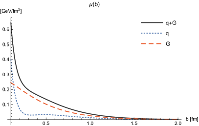
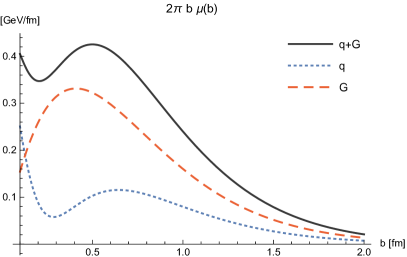
(a)                                                           (b)

Figure 18: Plots of the two-dimensional Galilean energy density, (a) $\mu(b)$ and (b) $2\pi\,b\,\mu(b)$, using the multipole model (11) with parameters given in Table 1, see Eq. (107) for the definition in terms of GFFs.

The difference in the behavior around $b=0$ between the quark and gluon contributions comes from the fact $D_{g}(t)=0$ whereas $D_{q}(t)\neq 0$. One might also be at first sight puzzled by the fact that total LF energy is given by $\sum_{a}\int\mathrm{d}^{2}b_{\perp}\,\mu_{a}(b)=M/2$ instead of $M$. This simply comes from our definition of the LF components which implies that $\int\mathrm{d}^{3}\tilde{x}\,\mathcal{T}^{+-}(\tilde{\boldsymbol{x}};\tilde{\boldsymbol{P}})=M^{2}/2P^{+}$.

IV.4 Infinite-momentum frame

In Ref. Brodsky:2006in ; Brodsky:2006ku three-dimensional LF distributions for finite $P^{+}$ have been defined by means of a Fourier transform with respect to the longitudinal LF boost-invariant skewness variable $\xi=-\Delta^{+}/2P^{+}$ instead of $\Delta^{+}$. The problem with these distributions is that the (quasi-)probabilistic interpretation is lost owing to the non-vanishing LF energy transfer $\Delta^{-}\neq 0$. Moreover, the center of the target with respect to which the transverse coordinates are defined differs between the initial and final states when $\xi\neq 0$ Diehl:2002he .

The above issues disappear when $\xi=0$. In the literature, one usually considers finite $P^{+}$ and hence $\Delta^{+}=0$, reducing the LF distributions to two spatial dimensions. This option was discussed in the previous section. The other possibility is to consider $P^{+}\gg\Delta^{+},\sqrt{P^{2}}$, i.e. the IMF within the LF formalism. In this case, we can formally define another type of three-dimensional LF distributions free of the aforementioned problems. To the best of our knowledge, this is the first time that such an option is explored. The reason can likely be attributed to the fact that one usually has in mind reaching the IMF through an infinite longitudinal boost. In that case, both $P^{+}$ and $\Delta^{+}$ will get large with their ratio $\xi$ fixed. Actually, one should just consider $P^{+}\to\infty$ with $\Delta^{+}$ fixed. The information about the longitudinal spatial structure is then encoded around $\xi\approx 0$.

Expanding the unpolarized off-forward LF amplitude (100) in powers of $1/P^{+}$, we find

$$\langle\!\langle T^{\mu\nu}_{a}(0)\rangle\!\rangle =P^{+}\,\eta^{\mu-}\eta^{\nu-}\left\{A_{a}(t)-\frac{(\Delta^{+})^{2}}{4(P^{+})^{2}}\left[\tfrac{1}{2}\,A_{a}(t)+B_{a}(t)\right]\right\}$$ (112)

$$+\frac{M}{P^{+}}\left\{M\,\eta^{-\{\mu}\eta^{\nu\}+}\,\frac{A_{a}(t)}{2}+\frac{\Delta^{\mu}\Delta^{\nu}+\eta^{\mu\nu}\boldsymbol{\Delta}^{2}_{\perp}}{M}\,C_{a}(t)+M\eta^{\mu\nu}\bar{C}_{a}(t)\right\}$$

$$-\frac{\boldsymbol{\Delta}^{2}_{\perp}}{4P^{+}}\left\{\eta^{-\{\mu}\eta^{\nu\}+}\,\frac{B_{a}(t)}{2}+\eta^{-[\mu}\eta^{\nu]+}\,\frac{D_{a}(t)}{2}\right\}$$

$$-\frac{\Delta^{+}}{4P^{+}}\left\{\eta^{-\{\mu}\Delta^{\nu\}}_{\perp}\,\frac{A_{a}(t)+B_{a}(t)}{2}+\eta^{-[\mu}\Delta^{\nu]}_{\perp}\,\frac{D_{a}(t)}{2}\right\}+\mathcal{O}(1/(P^{+})^{2})\,.$$

Its Fourier transform $\mathcal{T}^{\mu\nu}_{a}$ can be expressed in terms of 3-dimensional Fourier transforms of GFFs. The expression we obtain is however so complicated that we were not able to recognize the EMT structure of any known continuous medium discussed in the literature. Note also that since $\Delta^{-}\propto 1/(P^{+})^{2}$, we can write $t\approx-\boldsymbol{\Delta}^{2}_{\perp}$. The GFFs therefore do not contribute to the $\Delta^{+}$-dependence in the LF IMF and the longitudinal structure is essentially determined by Lorentz symmetry. As a final remark, we naturally recover the DYF results in the limit $\Delta^{+}\to 0$. This means that the projection of the distributions defined in the LF IMF onto the transverse plane coincides with the two-dimensional distributions defined in the DYF.

V Discussion

Having defined the notions of energy density and pressure inside the nucleon, we can go on and discuss the questions of hydrostatic equilibrium and stability constraints. While the former are automatically satisfied once GFFs are determined, the latter provide new constraints particularly useful for the phenomenology of high-energy scatterings involving nucleons.

V.1 Hydrostatic equilibrium

V.1.1 Three-dimensional case

Conservation of the total EMT $\partial_{\mu}T^{\mu\nu}(x)=0$ implies that the static total EMT $\mathcal{T}^{\mu\nu}=\sum_{a}\mathcal{T}^{\mu\nu}_{a}$ satisfies in the BF

$$\nabla^{i}\mathcal{T}^{ij}(\boldsymbol{r};\boldsymbol{0})=0\,,$$ (113)

or equivalently

$$\frac{\mathrm{d}p_{r}(r)}{\mathrm{d}r}=-\frac{2s(r)}{r},$$ (114)

which is the equation of hydrostatic equilibrium in the presence of pressure anisotropy. The RHS of Eq. (114) represents the effects of a force arising from the anisotropic nature of the medium. When $p_{r}(r)<p_{t}(r)$, we get $s(r)<0$ and the force is repulsive. When $p_{r}(r)>p_{t}(r)$, we get $s(r)>0$ and the force is attractive. This force is the mechanical origin of the surface tension between a liquid and its vapor Marchand:2011 . In the bulk of ordinary fluids, the density is essentially constant and the pressure is isotropic. The density changes however drastically across the interface, and generates an asymmetry in the stress tensor which can be understood as arising from a difference of ranges between attractive and repulsive interactions. The interface being usually extremely thin for ordinary fluids, the asymmetry can usually be modelled by a simple surface tension. This picture is supported by a molecular dynamics simulation of molecules interacting via a Lennard-Jones potential Marchand:2011 ; Weijs:2011 , which shows that the transition in the time-averaged density profile from the high-density liquid to the low-density gas takes place in a very narrow region that is a few molecules wide. At the same time, the profile of the stress anisotropy indicates that there is a force localized in the same narrow region acting in the direction parallel to the interface.

If $r$ is the coordinate normal to the interface, the surface tension $\gamma$ is obtained from the Bakker equation bakker:1928 (also known as the Kirkwood and Buff method Kirkwood:1949 )

$$\gamma=\int_{D}\mathrm{d}r\,s(r),$$ (116)

where $D$ is the domain where $s(r)$ is significant. When the domain is very narrow, we can make the approximation $s(r)\approx\gamma\,\delta(r-R)$. Integrating then the equation of hydrostatic equilibrium (114) over the radial coordinate yields the well-known Young-Laplace relation $p_{r}(0)=2\gamma/R$ for a spherical drop with radius $R$ Thomson:1958 . For compact stars and hadrons, the anisotropic stress spreads over a significant fraction of the volume of the system and cannot be realistically approximated by a delta function.

Many relations can be derived from Eq. (114), as discussed in Goeke:2007fp ; Polyakov:2018zvc . Let $f(r)$ be some radial function, one finds using integration by parts

$$\left[f(r)\,p_{r}(r)\right]_{0}^{\infty}=\int_{0}^{\infty}\mathrm{d}r\left[\frac{\mathrm{d}f(r)}{\mathrm{d}r}\,p_{r}(r)-2\,\frac{f(r)}{r}\,s(r)\right].$$ (117)

For $f(r)=1$, one obtains the generalized Young-Laplace relation

$$p_{r}(0)=2\int_{0}^{\infty}\mathrm{d}r\,\frac{s(r)}{r}.$$ (118)

If $p_{r}(r)$ is finite at $r=0$ and decays faster than $1/r^{N}$ with $N>0$ for $r\to\infty$, the choice $f(r)=r^{N}$ leads to

$$\int_{0}^{\infty}\mathrm{d}r\,r^{N-1}\left[Np_{r}(r)-2s(r)\right]=0\,.$$ (119)

The case $N=3$ is known as the von Laue condition Laue:1911lrk

$$\int_{0}^{\infty}\mathrm{d}r\,r^{2}\,p(r)=0\,,$$ (120)

and indicates that the isotropic pressure has to change sign. We illustrate this in Fig. 19 using the multipole model (11) with parameters given in Table 1.

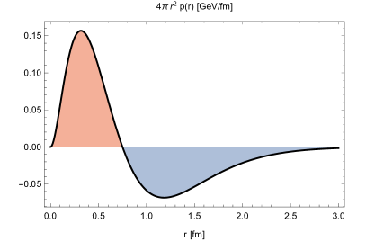
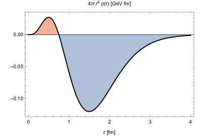
(a)                                                           (b)

Figure 19: Illustration of the hydrostatic equilibrium in the Breit frame. (a) integrand of the von Laue condition (120) and (b) the same integrand multiplied by $r^{2}$.

As one can see from panel (a) showing the integrand of the von Laue condition (120), the net positive pressure (i.e. repulsive force) of the inner region is exactly balanced by the net negative pressure (i.e. attractive force) of the outer region. Multiplying this integrand by an additional factor $r^{2}$ as in Eq. (48) explains why the gravitational charge $C(0)$ turns out to be negative.

Similarly, the case $N=2$

$$\int_{0}^{\infty}\mathrm{d}r\,r\,p_{t}(r)=0$$ (121)

indicates that the tangential pressure also changes sign. The net tangential force in the inner region is repulsive whereas it is negative in the outer region, leading once more to the conclusion that $C(0)<0$ based on Eq. (48). The other remarkable values are $N=1,\frac{6}{5},\frac{12}{5},4,6$

$$\int_{0}^{\infty}\mathrm{d}r\,p_{t}(r) =\int_{0}^{\infty}\mathrm{d}r\,s(r)\,,$$ (122)

$$\int_{0}^{\infty}\mathrm{d}r\,r^{1/5}\,p(r) =\int_{0}^{\infty}\mathrm{d}r\,r^{1/5}\,s(r)\,,$$ (123)

$$\int_{0}^{\infty}\mathrm{d}r\,r^{7/5}\,p(r) =-\int_{0}^{\infty}\mathrm{d}r\,r^{7/5}\,p_{t}(r)\,,$$ (124)

$$\int_{0}^{\infty}\mathrm{d}r\,r^{3}\,p_{r}(r) =-\int_{0}^{\infty}\mathrm{d}r\,r^{3}\,p_{t}(r)\,,$$ (125)

$$\int_{0}^{\infty}\mathrm{d}r\,r^{5}\,p(r) =-\int_{0}^{\infty}\mathrm{d}r\,r^{5}\,p_{r}(r)\,.$$ (126)

All the above relations are automatically satisfied by our expressions (35) and (38) when summed over the constituents. The reason for this is that the parametrization (8) together with the sum rules (9) already encode the conservation of the total EMT, implying that the equation of hydrostatic equilibrium (114) is identically satisfied. These relations can however be particularly useful to test model predictions where full Lorentz covariance are often absent.

V.1.2 Two-dimensional case

The discussion in the EF proceeds analogously to the BF. The main difference is that the spatial distributions are now two-dimensional instead of three-dimensional. Note also that since the two-dimensional pressure distributions are the same in both EF (with $P_{z}=0$ or $P_{z}\to\infty$) and DYF, the following results apply to both instant and front forms.

Using the conservation of the static total EMT in two dimensions

$$\nabla^{i}_{\perp}\mathsf{T}^{ij}(\boldsymbol{b}_{\perp};\boldsymbol{0})=0\,,$$ (127)

we find that the equation of hydrodynamic equilibrium in the EF takes the form

$$\frac{\mathrm{d}\sigma_{r}(b)}{\mathrm{d}b}=-\frac{\Pi(b)}{b}\,,$$ (128)

where we omitted the $P_{z}$-dependence for convenience. If $f(b)$ is some radial function, we obtain using integration by parts

$$\left[f(b)\,\sigma_{r}(b)\right]_{0}^{\infty}=\int_{0}^{\infty}\mathrm{d}b\left[\frac{\mathrm{d}f(b)}{\mathrm{d}b}\,\sigma_{r}(b)-\frac{f(b)}{b}\,\Pi(b)\right].$$ (129)

For $f(b)=1$, we get

$$\sigma_{r}(0)=\int_{0}^{\infty}\mathrm{d}b\,\frac{\Pi(b)}{b}\,.$$ (130)

When the pressure anisotropy is concentrated within a thin region, it can be approximated by $\Pi(b)\approx\tau\,\delta(b-R)$. Equation (130) reduces then to the two-dimensional version of the Young-Laplace relation $\sigma_{r}(0)=\tau/R$, where $\tau$ can be thought of as some sort of effective string tension. More generally, the effective string tension can be defined from the two-dimensional version of the Bakker equation

$$\tau=\int_{D}\mathrm{d}b\,\Pi(b).$$ (131)

If $\sigma_{r}(b)$ is finite at $b=0$ and decays faster than $1/b^{N}$ with $N>0$ for $b\to\infty$, the choice $f(b)=b^{N}$ leads to

$$\int_{0}^{\infty}\mathrm{d}b\,b^{N-1}\left[N\sigma_{r}(b)-\Pi(b)\right]=0\,.$$ (132)

The case $N=2$ corresponds to the two-dimensional version of the von Laue condition

$$\int_{0}^{\infty}\mathrm{d}b\,b\,\sigma(b)=0\,,$$ (133)

and indicates that the isotropic pressure has to change sign. We illustrate this in Fig. 20 using the multipole model (11) with parameters given in Table 1.

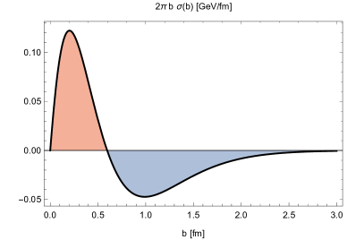
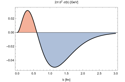
(a)                                                           (b)

Figure 20: Illustration of the hydrostatic equilibrium in the elastic frame. (a) integrand of the two-dimensional von Laue condition (133) and (b) the same integrand multiplied by $b$.

As one can see from panel (a) showing the integrand of the two-dimensional version of the von Laue condition (133), the picture is similar to the one in the BF. Namely, the net positive pressure of the inner region is exactly balanced by the net negative pressure of the outer region. Multiplying this integrand by an additional factor $b$ as in Eq. (72) explains why the gravitational charge $C(0)$ turns out to be negative.

Similarly, the case $N=1$

$$\int_{0}^{\infty}\mathrm{d}b\,\sigma_{t}(b)=0$$ (134)

indicates that the tangential pressure also changes sign. Once again, the net tangential force in the inner region is repulsive whereas it is negative in the outer region, in agreement with $C(0)<0$ according to Eq. (72). The other remarkable values are $N=\frac{1}{2},\frac{2}{3},\frac{4}{3},4$

$$\int_{0}^{\infty}\mathrm{d}b\,b^{-1/2}\,\sigma_{t}(b) =\int_{0}^{\infty}\mathrm{d}b\,b^{-1/2}\,\Pi(b)\,,$$ (135)

$$\int_{0}^{\infty}\mathrm{d}b\,b^{-1/3}\,\sigma(b) =\int_{0}^{\infty}\mathrm{d}b\,b^{-1/3}\,\Pi(b)\,,$$ (136)

$$\int_{0}^{\infty}\mathrm{d}b\,b^{1/3}\,\sigma(b) =-\int_{0}^{\infty}\mathrm{d}b\,b^{1/3}\,\sigma_{t}(b)\,,$$ (137)

$$\int_{0}^{\infty}\mathrm{d}b\,b^{3}\,\sigma(b) =-\int_{0}^{\infty}\mathrm{d}b\,b^{3}\,\sigma_{r}(b)\,.$$ (138)

For the same reason as in the three-dimensional case, all the above relations are automatically satisfied by our expressions (59) and (60) when summed over the constituents.

V.2 Stability

We have seen earlier that the study of the nucleon EMT might provide some clues about the EoS for the matter lying in the heart of compact stars. The stability of compact stars made of anisotropic matter has been extensively discussed in Herrera:1992lwz ; Herrera:1997plx ; Abreu:2007ew . We suggest that applying these results to the case of the nucleon can in turn provide new constraints on the nucleon EMT, and hence on the GPDs.

For a stable system, it is expected that

(i) $$\varepsilon(0)<\infty,\ p(0)<\infty\ \text{and}\ s(0)=0\,;$$ (139)

(ii) $$\varepsilon(r)>0\ \text{and}\ p_{r}(r)>0\,;$$ (140)

(iii) $$\frac{\mathrm{d}\varepsilon(r)}{\mathrm{d}r}<0\ \text{and}\ \frac{\mathrm{d}p_{r}(r)}{\mathrm{d}r}<0\,.$$ (141)

All these constraints are satisfied by our simple multipole model (11) with parameters given in Table 1. We observe in particular that the constraint (i) rules out the dipole Ansatz for the GFFs $B_{a}(t)$ and $C_{a}(t)$ sometimes used in the literature, because it generates a $1/r$ pole in $\varepsilon(r)$ and $p(r)$, and leads to $s(0)\neq 0$. We therefore used in our simple multipole model the tripole Ansatz which does not have the same problem and which agrees with the asymptotic behaviour expected from the quark counting rules Matveev:1973ra ; Brodsky:1973kr ; Brodsky:1974vy ; Lepage:1980fj .

It is also expected that the (squared) radial and tangential speeds of sound defined as $v^{2}_{sr}(r)=\frac{\mathrm{d}p_{r}(r)/\mathrm{d}r}{\mathrm{d}\varepsilon(r)/\mathrm{d}r}$ and $v^{2}_{st}(r)=\frac{\mathrm{d}p_{t}(r)/\mathrm{d}r}{\mathrm{d}\varepsilon(r)/\mathrm{d}r}$ satisfy

(iv) $$0\leq v^{2}_{sr}(r)\leq 1\ \text{and}\ 0\leq v^{2}_{st}(r)\leq 1\,;$$ (142)

(v) $$|v^{2}_{st}(r)-v^{2}_{sr}(r)|\leq 1\,;$$ (143)

(vi) $$\Gamma(r)=\frac{\varepsilon(r)+p_{r}(r)}{p_{r}(r)}\,v^{2}_{sr}>\frac{4}{3}\,.$$ (144)

Violations of these additional constraints are observed over some range in $r$ within our simple multipole model.

Finally, there exist also energy conditions which reflect the principles of relativity and play an important role in General Relativity. They constitute an essential ingredient for establishing general results like the no-hair theorem, the laws of black hole thermodynamics or the singularity theorems of Penrose and Hawking Hawking:1973uf ; Wald:1984rg ; Poisson:2009pwt ; Senovilla:2014gza ; Curiel:2014zba ; Martin-Moruno:2017exc ; Maeda:2018hqu . The most popular ones are the Null Energy Condition (NEC), Weak Energy Condition (WEC), Strong Energy Condition (SEC), and Dominant Energy Condition (DEC)

NEC $$\varepsilon(r)+p_{i}(r) \geq 0\,,$$ (145)

WEC $$\varepsilon(r)+p_{i}(r) \geq 0\qquad\text{and}\qquad\varepsilon(r)\geq 0\,,$$ (146)

SEC $$\varepsilon(r)+p_{i}(r) \geq 0\qquad\text{and}\qquad\varepsilon(r)+3\,p(r)\geq 0\,,$$ (147)

DEC $$\varepsilon(r) \geq|p_{i}(r)|,$$ (148)

where $i=r,t$. Some of these energy conditions have a simple physical interpretation. Namely, the weak energy condition arises from the requirement that the energy density is non-negative for any observer, and the dominant energy condition ensures that the energy flow cannot exceed the speed of light for any observer. All known forms of matter so far satisfy these energy conditions. Our simple multipole model (11) with parameters given in Table 1 also satisfy these energy conditions except the SEC $\varepsilon(r)+3\,p(r)\geq 0$ for some range in $r$.

All the above conditions on the distributions of energy density and pressure are extremely interesting since, when transposed to the nucleon case using our expressions (34)-(38), they can provide new phenomenological constraints on the GFFs and hence on the GPDs of the nucleon. Recently, criterion (ii) has been considered in Perevalova:2016dln and led to the conclusion that $C(0)$ should be negative owing to Eq. (48). We note that this agrees with criterion (iii) which implies that $s(r)>0$ (as assumed in Goeke:2007fp ) using the equation of hydrostatic equilibrium (114), and in turn $C(0)<0$ according to Eq. (47). Note also that the inequalities can in principle be easily transposed to the two-dimensional case, which in conjunction with our expressions (56)-(60), may lead to yet further new constraints on the GPDs.

Satisfying all the constraints at the same time is not at all a trivial task. Some may even perhaps be unapplicable to the nucleon case. For these reasons, we refrain from developing here a more realistic model since its main purpose in the present study was only to illustrate the various distributions. A detailed analysis of the stability constraints in the hadronic context goes beyond the scope of the present paper and is left for future investigations.

VI Conclusions

We revisited the interpretation of spin-1/2 gravitational form factors in terms of the mechanical properties of hadrons. We rederived and significantly extended the existing literature, which so far has been exploiting only the Breit frame and the instant form of dynamics. In particular we discussed here both the instant and front forms of dynamics, and the separate quark and gluon contributions to the energy and pressure distributions in the Breit, elastic, infinite-momentum and Drell-Yan frames. Our key results are contained in Eqs. (34)–(38) for the Breit frame, Eqs. (56)–(60) for the elastic frame, and Eqs. (107)–(111) for the Drell-Yan frame. We illustrated our argument with a simple phenomenological model, and highlighted the constraints coming from mechanical properties that should generically be satisfied in model-building.

We put a special emphasis on the pressure anisotropy, which offers an innovative perspective on the nucleon structure from our rapidly growing knowledge on compact stellar objects. The direct observation of neutron star mergers in terrestrial gravitational wave observatories indeed already brought constraints on the equation of state of nuclear matter at high density and low temperature. Orders of magnitude and model studies suggest that the nucleon itself may be described with the same concepts and pictures. In particular, the stability and hydrostatic equilibrium conditions are presumably the best theoretical ingredients to elaborate on this picture since most of the gravitational form factors are within contemporary experimental reach through hard exclusive experiments and generalized parton distributions. However, determining how much we can learn about the physics of compact stars from the nucleon structure (or conversely) is still an exciting open question.

References

- (1) Xiang-Dong Ji, “Gauge-Invariant Decomposition of Nucleon Spin,” Phys. Rev. Lett. 78, 610–613 (1997), arXiv:hep-ph/9603249 [hep-ph]
- (2) Xiang-Dong Ji, “Deeply virtual Compton scattering,” Phys. Rev. D55, 7114–7125 (1997), arXiv:hep-ph/9609381 [hep-ph]
- (3) A. Accardi et al., “Electron Ion Collider: The Next QCD Frontier,” Eur. Phys. J. A52, 268 (2016), arXiv:1212.1701 [nucl-ex]
- (4) Yi-Bo Yang, Ming Gong, Jian Liang, Huey-Wen Lin, Keh-Fei Liu, Dimitra Pefkou, and Phiala Shanahan, “Nonperturbatively renormalized glue momentum fraction at the physical pion mass from lattice QCD,” Phys. Rev. D98, 074506 (2018), arXiv:1805.00531 [hep-lat]
- (5) Constantia Alexandrou, Martha Constantinou, Kyriakos Hadjiyiannakou, Karl Jansen, Christos Kallidonis, Giannis Koutsou, and Alejandro Vaquero Avilés-Casco, “Nucleon spin structure from lattice QCD,” Proceedings, 26th International Workshop on Deep Inelastic Scattering and Related Subjects (DIS 2018): Port Island, Kobe, Japan, April 16-20, 2018, PoS DIS2018, 148 (2018), arXiv:1807.11214 [hep-lat]
- (6) Yi-Bo Yang, Jian Liang, Yu-Jiang Bi, Ying Chen, Terrence Draper, Keh-Fei Liu, and Zhaofeng Liu, “Proton Mass Decomposition from the QCD Energy Momentum Tensor,” Phys. Rev. Lett. 121, 212001 (2018), arXiv:1808.08677 [hep-lat]
- (7) P. E. Shanahan and W. Detmold, “Gluon gravitational form factors of the nucleon and the pion from lattice QCD,” (2018), arXiv:1810.04626 [hep-lat]
- (8) P. E. Shanahan and W. Detmold, “The pressure distribution and shear forces inside the proton,” (2018), arXiv:1810.07589 [nucl-th]
- (9) A. Pais and S. T. Epstein, “Note on Relativistic Properties of Self-Energies,” Rev. Mod. Phys. 21, 445–446 (1949)
- (10) M. V. Polyakov, “Generalized parton distributions and strong forces inside nucleons and nuclei,” Phys. Lett. B555, 57–62 (2003), arXiv:hep-ph/0210165 [hep-ph]
- (11) Maxim V. Polyakov and Peter Schweitzer, “Forces inside hadrons: pressure, surface tension, mechanical radius, and all that,” Int. J. Mod. Phys. A33, 1830025 (2018), arXiv:1805.06596 [hep-ph]
- (12) M. Ruderman, “Pulsars: structure and dynamics,” Ann. Rev. Astron. Astrophys. 10, 427–476 (1972)
- (13) V. Canuto, “Equation of State at Ultrahigh Densities. 1..” Ann. Rev. Astron. Astrophys. 12, 167–214 (1974)
- (14) Charles Alcock, Edward Farhi, and Angela Olinto, “Strange stars,” Astrophys. J. 310, 261–272 (1986)
- (15) P. Haensel, J. L. Zdunik, and R. Schaeffer, “Strange quark stars,” Astron. Astrophys. 160, 121–128 (1986)
- (16) Fridolin Weber, “Strange quark matter and compact stars,” Prog. Part. Nucl. Phys. 54, 193–288 (2005), arXiv:astro-ph/0407155 [astro-ph]
- (17) M. Angeles Perez-Garcia, Joseph Silk, and Jirina R. Stone, “Dark matter, neutron stars and strange quark matter,” Phys. Rev. Lett. 105, 141101 (2010), arXiv:1007.1421 [astro-ph.CO]
- (18) Hilario Rodrigues, Sergio Barbosa Duarte, and Jose Carlos T. De Oliveira, “Massive compact stars as quark stars,” Astrophys. J. 730, 31 (2011), arXiv:1407.4704 [astro-ph.HE]
- (19) Richard L. Bowers and E. P. T. Liang, “Anisotropic Spheres in General Relativity,” Astrophys. J. 188, 657–665 (1974)
- (20) L. Herrera and N. O. Santos, “Local anisotropy in self-gravitating systems,” Phys. Rept. 286, 53–130 (1997)
- (21) M. K. Mak and T. Harko, “Anisotropic stars in general relativity,” Proc. Roy. Soc. Lond. A459, 393–408 (2003), arXiv:gr-qc/0110103 [gr-qc]
- (22) Krsna Dev and Marcelo Gleiser, “Anisotropic stars: Exact solutions,” Gen. Rel. Grav. 34, 1793–1818 (2002), arXiv:astro-ph/0012265 [astro-ph]
- (23) Krsna Dev and Marcelo Gleiser, “Anisotropic stars. 2. Stability,” Gen. Rel. Grav. 35, 1435–1457 (2003), arXiv:gr-qc/0303077 [gr-qc]
- (24) Hector O. Silva, Caio F. B. Macedo, Emanuele Berti, and Luís C. B. Crispino, “Slowly rotating anisotropic neutron stars in general relativity and scalar–tensor theory,” Class. Quant. Grav. 32, 145008 (2015), arXiv:1411.6286 [gr-qc]
- (25) C. G. Boehmer and T. Harko, “Bounds on the basic physical parameters for anisotropic compact general relativistic objects,” Class. Quant. Grav. 23, 6479–6491 (2006), arXiv:gr-qc/0609061 [gr-qc]
- (26) K. Goeke, J. Grabis, J. Ossmann, M. V. Polyakov, P. Schweitzer, A. Silva, and D. Urbano, “Nucleon form-factors of the energy momentum tensor in the chiral quark-soliton model,” Phys. Rev. D75, 094021 (2007), arXiv:hep-ph/0702030 [hep-ph]
- (27) Matthias Burkardt, “Impact parameter space interpretation for generalized parton distributions,” Int. J. Mod. Phys. A18, 173–208 (2003), arXiv:hep-ph/0207047 [hep-ph]
- (28) E. Leader and C. Lorcé, “The angular momentum controversy: What’s it all about and does it matter?.” Phys. Rept. 541, 163–248 (2014), arXiv:1309.4235 [hep-ph]
- (29) Cédric Lorcé, Luca Mantovani, and Barbara Pasquini, “Spatial distribution of angular momentum inside the nucleon,” Phys. Lett. B776, 38–47 (2018), arXiv:1704.08557 [hep-ph]
- (30) M. Hillery, R. F. O’Connell, M. O. Scully, and Eugene P. Wigner, “Distribution functions in physics: Fundamentals,” Phys. Rept. 106, 121–167 (1984)
- (31) F. Villars, “On the Energy-Momentum Tensor of the Electron,” Phys. Rev. 79, 122–128 (1950)
- (32) I. Yu. Kobzarev and L. B. Okun, “GRAVITATIONAL INTERACTION OF FERMIONS,” Zh. Eksp. Teor. Fiz. 43, 1904–1909 (1962), [Sov. Phys. JETP16,1343 (1963)]
- (33) I. Yu. Kobzarev and L. B. Okun, “GRAVITATIONAL INTERACTION OF FERMIONS,” Sov. Phys. JETP 16, 1343 (1963), [Zh. Eksp. Teor. Fiz.43, 1904 (1962)]
- (34) Heinz Pagels, “Energy-Momentum Structure Form Factors of Particles,” Phys. Rev. 144, 1250–1260 (1966)
- (35) B. L. G. Bakker, E. Leader, and T. L. Trueman, “A Critique of the angular momentum sum rules and a new angular momentum sum rule,” Phys. Rev. D70, 114001 (2004), arXiv:hep-ph/0406139 [hep-ph]
- (36) Cédric Lorcé, “The light-front gauge-invariant energy-momentum tensor,” JHEP 08, 045 (2015), arXiv:1502.06656 [hep-ph]
- (37) O. V. Teryaev, “Spin structure of nucleon and equivalence principle,” (1999), arXiv:hep-ph/9904376 [hep-ph]
- (38) Peter Lowdon, Kelly Yu-Ju Chiu, and Stanley J. Brodsky, “Rigorous constraints on the matrix elements of the energy-momentum tensor,” Phys. Lett. B774, 1–6 (2017), arXiv:1707.06313 [hep-th]
- (39) O. V. Teryaev, “Gravitational form factors and nucleon spin structure,” Front. Phys.(Beijing) 11, 111207 (2016)
- (40) Stanley J. Brodsky, Dae Sung Hwang, Bo-Qiang Ma, and Ivan Schmidt, “Light cone representation of the spin and orbital angular momentum of relativistic composite systems,” Nucl. Phys. B593, 311–335 (2001), arXiv:hep-th/0003082 [hep-th]
- (41) Hyun-Chul Kim, Peter Schweitzer, and Ulugbek Yakhshiev, “Energy-momentum tensor form factors of the nucleon in nuclear matter,” Phys. Lett. B718, 625–631 (2012), arXiv:1205.5228 [hep-ph]
- (42) Ph. Hagler et al. (LHPC), “Nucleon Generalized Parton Distributions from Full Lattice QCD,” Phys. Rev. D77, 094502 (2008), arXiv:0705.4295 [hep-lat]
- (43) Gunnar Bali, Sara Collins, Meinulf Göckeler, Rudolf Rödl, Andreas Schäfer, and Andre Sternbeck, “Nucleon generalized form factors from lattice QCD with nearly physical quark masses,” Proceedings, 33rd International Symposium on Lattice Field Theory (Lattice 2015): Kobe, Japan, July 14-18, 2015, PoS LATTICE2015, 118 (2016), arXiv:1601.04818 [hep-lat]
- (44) C. Alexandrou, M. Constantinou, K. Hadjiyiannakou, K. Jansen, C. Kallidonis, G. Koutsou, A. Vaquero Avilés-Casco, and C. Wiese, “Nucleon Spin and Momentum Decomposition Using Lattice QCD Simulations,” Phys. Rev. Lett. 119, 142002 (2017), arXiv:1706.02973 [hep-lat]
- (45) Xiang-Dong Ji, “Off forward parton distributions,” J. Phys. G24, 1181–1205 (1998), arXiv:hep-ph/9807358 [hep-ph]
- (46) Dieter Müller, D. Robaschik, B. Geyer, F. M. Dittes, and J. Hoeji, “Wave functions, evolution equations and evolution kernels from light ray operators of QCD,” Fortsch. Phys. 42, 101–141 (1994), arXiv:hep-ph/9812448 [hep-ph]
- (47) A.V. Radyushkin, “Scaling limit of deeply virtual Compton scattering,” Phys.Lett. B380, 417–425 (1996), arXiv:hep-ph/9604317 [hep-ph]
- (48) Kresimir Kumericki, Simonetta Liuti, and Herve Moutarde, “GPD phenomenology and DVCS fitting,” Eur. Phys. J. A52, 157 (2016), arXiv:1602.02763 [hep-ph]
- (49) L. Favart, M. Guidal, T. Horn, and P. Kroll, “Deeply Virtual Meson Production on the nucleon,” Eur. Phys. J. A52, 158 (2016), arXiv:1511.04535 [hep-ph]
- (50) S. Kumano, Qin-Tao Song, and O. V. Teryaev, “Hadron tomography by generalized distribution amplitudes in pion-pair production process and gravitational form factors for pion,” Phys. Rev. D97, 014020 (2018), arXiv:1711.08088 [hep-ph]
- (51) Elliot Leader, “A critical assessment of the angular momentum sum rules,” Phys. Lett. B720, 120–124 (2013), [Erratum: Phys. Lett.B726,927(2013)], arXiv:1211.3957 [hep-ph]
- (52) Kazuhiro Tanaka, “Operator relations for gravitational form factors of a spin-0 hadron,” Phys. Rev. D98, 034009 (2018), arXiv:1806.10591 [hep-ph]
- (53) J. M. Alarcon, J. Martin Camalich, and J. A. Oller, “The chiral representation of the scattering amplitude and the pion-nucleon sigma term,” Phys. Rev. D85, 051503 (2012), arXiv:1110.3797 [hep-ph]
- (54) Martin Hoferichter, J. Ruiz de Elvira, Bastian Kubis, and Ulf-G. Meißner, “High-Precision Determination of the Pion-Nucleon Term from Roy-Steiner Equations,” Phys. Rev. Lett. 115, 092301 (2015), arXiv:1506.04142 [hep-ph]
- (55) D. E. Kharzeev and J. Raufeisen, “High-energy nuclear interactions and QCD: An Introduction,” New states of matter in hadronic interactions. Proceedings, Pan-American Advanced Study Institute, PASI 2002, Campos do Jordao, Sao Paulo, Brazil, January 7-18, 2002, AIP Conf. Proc. 631, 27–69 (2002), arXiv:nucl-th/0206073 [nucl-th]
- (56) G. Krein, A. W. Thomas, and K. Tsushima, “Nuclear-bound quarkonia and heavy-flavor hadrons,” Prog. Part. Nucl. Phys. 100, 161–210 (2018), arXiv:1706.02688 [hep-ph]
- (57) S. Joosten and Z. E. Meziani, “Heavy Quarkonium Production at Threshold: from JLab to EIC,” Proceedings, QCD Evolution Workshop (QCD 2017): Newport News, VA, USA, May 22-26, 2017, PoS QCDEV2017, 017 (2018), arXiv:1802.02616 [hep-ex]
- (58) Sylvester Joosten, “Probing the gluonic structure of the nucleon through quarkonium production,” (2018), arXiv:1803.08615 [hep-ph]
- (59) Yoshitaka Hatta and Di-Lun Yang, “Holographic production near threshold and the proton mass problem,” Phys. Rev. D98, 074003 (2018), arXiv:1808.02163 [hep-ph]
- (60) Veronique Bernard, Latifa Elouadrhiri, and Ulf-G. Meissner, “Axial structure of the nucleon: Topical Review,” J. Phys. G28, R1–R35 (2002), arXiv:hep-ph/0107088 [hep-ph]
- (61) L. A. Harland-Lang, A. D. Martin, P. Motylinski, and R. S. Thorne, “Parton distributions in the LHC era: MMHT 2014 PDFs,” Eur. Phys. J. C75, 204 (2015), arXiv:1412.3989 [hep-ph]
- (62) Chandan Mondal, “Longitudinal momentum densities in transverse plane for nucleons,” Eur. Phys. J. C76, 74 (2016), arXiv:1511.01736 [hep-ph]
- (63) Narinder Kumar, Chandan Mondal, and Neetika Sharma, “Gravitational form factors and angular momentum densities in light-front quark-diquark model,” Eur. Phys. J. A53, 237 (2017), arXiv:1712.02110 [hep-ph]
- (64) M. Deka et al., “Lattice study of quark and glue momenta and angular momenta in the nucleon,” Phys. Rev. D91, 014505 (2015), arXiv:1312.4816 [hep-lat]
- (65) B. Pasquini, M. V. Polyakov, and M. Vanderhaeghen, “Dispersive evaluation of the D-term form factor in deeply virtual Compton scattering,” Phys. Lett. B739, 133–138 (2014), arXiv:1407.5960 [hep-ph]
- (66) V. D. Burkert, L. Elouadrhiri, and F. X. Girod, “The pressure distribution inside the proton,” Nature 557, 396–399 (2018)
- (67) Cédric Lorcé, “On the hadron mass decomposition,” Eur. Phys. J. C78, 120 (2018), arXiv:1706.05853 [hep-ph]
- (68) A. Airapetian et al. (HERMES), “Precise determination of the spin structure function g(1) of the proton, deuteron and neutron,” Phys. Rev. D75, 012007 (2007), arXiv:hep-ex/0609039 [hep-ex]
- (69) Maxim V. Polyakov and Hyeon-Dong Son, “Nucleon gravitational form factors from instantons: forces between quark and gluon subsystems,” JHEP 09, 156 (2018), arXiv:1808.00155 [hep-ph]
- (70) Constantia Alexandrou, Martha Constantinou, Kyriakos Hadjiyiannakou, Karl Jansen, Christos Kallidonis, Giannis Koutsou, and Alejandro Vaquero Aviles-Casco, “Nucleon axial form factors using = 2 twisted mass fermions with a physical value of the pion mass,” Phys. Rev. D96, 054507 (2017), arXiv:1705.03399 [hep-lat]
- (71) Cédric Lorcé, “The relativistic center of mass in field theory with spin,” Eur. Phys. J. C78, 785 (2018), arXiv:1805.05284 [hep-ph]
- (72) Cédric Lorcé, “New explicit expressions for Dirac bilinears,” Phys. Rev. D97, 016005 (2018), arXiv:1705.08370 [hep-ph]
- (73) Xiang-Dong Ji, “A QCD analysis of the mass structure of the nucleon,” Phys. Rev. Lett. 74, 1071–1074 (1995), arXiv:hep-ph/9410274 [hep-ph]
- (74) Xiang-Dong Ji, “Breakup of hadron masses and energy - momentum tensor of QCD,” Phys. Rev. D52, 271–281 (1995), arXiv:hep-ph/9502213 [hep-ph]
- (75) Carl Eckart, “The Thermodynamics of irreversible processes. 3.. Relativistic theory of the simple fluid,” Phys. Rev. 58, 919–924 (1940)
- (76) Haiyan Gao, Tianbo Liu, Chao Peng, Zhihong Ye, and Zhiwen Zhao, “Proton Remains Puzzling,” The Universe 3, 18–30 (2015)
- (77) Yoshitaka Hatta, Abha Rajan, and Kazuhiro Tanaka, “Quark and gluon contributions to the QCD trace anomaly,” JHEP 12, 008 (2018), arXiv:1810.05116 [hep-ph]
- (78) Xiang-Dong Ji, W. Melnitchouk, and X. Song, “A Study of off forward parton distributions,” Phys. Rev. D56, 5511–5523 (1997), arXiv:hep-ph/9702379 [hep-ph]
- (79) R. G. Sachs, “High-Energy Behavior of Nucleon Electromagnetic Form Factors,” Phys. Rev. 126, 2256–2260 (1962)
- (80) Selcuk S. Bayin, “Anisotropic fluids and cosmology,” Astrophys. J. 303, 101–110 (1986)
- (81) G. Lemaitre, “The expanding universe,” Annales Soc. Sci. Bruxelles A53, 51 (1933), [Gen. Rel. Grav. 29, 641 (1997)]
- (82) G. Lemaitre, “The expanding universe,” Gen. Rel. Grav. 29, 641–680 (1997), [Annales Soc. Sci. Bruxelles A53,51(1933)]
- (83) Randolf Pohl et al., “The size of the proton,” Nature 466, 213–216 (2010)
- (84) Randolf Pohl et al. (CREMA), “Laser spectroscopy of muonic deuterium,” Science 353, 669–673 (2016)
- (85) John Arrington, “An examination of proton charge radius extractions from e-p scattering data,” J. Phys. Chem. Ref. Data 44, 031203 (2015), arXiv:1506.00873 [nucl-ex]
- (86) I. A. Perevalova, M. V. Polyakov, and P. Schweitzer, “On LHCb pentaquarks as a baryon-(2S) bound state: prediction of isospin- pentaquarks with hidden charm,” Phys. Rev. D94, 054024 (2016), arXiv:1607.07008 [hep-ph]
- (87) Jonathan Hudson and Peter Schweitzer, “D term and the structure of pointlike and composed spin-0 particles,” Phys. Rev. D96, 114013 (2017), arXiv:1712.05316 [hep-ph]
- (88) Jonathan Hudson and Peter Schweitzer, “Dynamic origins of fermionic D-terms,” Phys. Rev. D97, 056003 (2018), arXiv:1712.05317 [hep-ph]
- (89) Feryal Özel and Paulo Freire, “Masses, Radii, and the Equation of State of Neutron Stars,” Ann. Rev. Astron. Astrophys. 54, 401–440 (2016), arXiv:1603.02698 [astro-ph.HE]
- (90) Pawel Danielewicz, Roy Lacey, and William G. Lynch, “Determination of the equation of state of dense matter,” Science 298, 1592–1596 (2002), arXiv:nucl-th/0208016 [nucl-th]
- (91) Luciano Rezzolla and Kentaro Takami, “Gravitational-wave signal from binary neutron stars: a systematic analysis of the spectral properties,” Phys. Rev. D93, 124051 (2016), arXiv:1604.00246 [gr-qc]
- (92) Eemeli Annala, Tyler Gorda, Aleksi Kurkela, and Aleksi Vuorinen, “Gravitational-wave constraints on the neutron-star-matter Equation of State,” Phys. Rev. Lett. 120, 172703 (2018), arXiv:1711.02644 [astro-ph.HE]
- (93) Vasileios Paschalidis, Kent Yagi, David Alvarez-Castillo, David B. Blaschke, and Armen Sedrakian, “Implications from GW170817 and I-Love-Q relations for relativistic hybrid stars,” Phys. Rev. D97, 084038 (2018), arXiv:1712.00451 [astro-ph.HE]
- (94) Elias R. Most, Lukas R. Weih, Luciano Rezzolla, and Jürgen Schaffner-Bielich, “New constraints on radii and tidal deformabilities of neutron stars from GW170817,” Phys. Rev. Lett. 120, 261103 (2018), arXiv:1803.00549 [gr-qc]
- (95) Rana Nandi, Prasanta Char, and Subrata Pal, “Constraining the equation of state with gravitational wave observation,” (2018), arXiv:1809.07108 [astro-ph.HE]
- (96) Alfredo Urbano and Hardi Veermäe, “On gravitational echoes from ultracompact exotic stars,” (2018), arXiv:1810.07137 [gr-qc]
- (97) Paul Demorest, Tim Pennucci, Scott Ransom, Mallory Roberts, and Jason Hessels, “Shapiro Delay Measurement of A Two Solar Mass Neutron Star,” Nature 467, 1081–1083 (2010), arXiv:1010.5788 [astro-ph.HE]
- (98) John Antoniadis et al., “A Massive Pulsar in a Compact Relativistic Binary,” Science 340, 6131 (2013), arXiv:1304.6875 [astro-ph.HE]
- (99) Subrahmanyan Chandrasekhar, “The maximum mass of ideal white dwarfs,” Astrophys. J. 74, 81–82 (1931)
- (100) G. Baym and S. A. Chin, “Can a Neutron Star Be a Giant MIT Bag?.” Phys. Lett. 62B, 241–244 (1976)
- (101) A. Drago, U. Tambini, and M. Hjorth-Jensen, “Neutron stars and massive quark matter,” Phys. Lett. B380, 13–17 (1996), arXiv:nucl-th/9505037 [nucl-th]
- (102) J. Rikovska-Stone, Pierre A. M. Guichon, Hrayr H. Matevosyan, and Anthony William Thomas, “Cold uniform matter and neutron stars in the quark-mesons-coupling model,” Nucl. Phys. A792, 341–369 (2007), arXiv:nucl-th/0611030 [nucl-th]
- (103) J. R. Stone, P. A. M. Guichon, and A. W. Thomas, “Role of Hyperons in Neutron Stars,” (2010), arXiv:1012.2919 [nucl-th]
- (104) T. F. Motta, P. A. M. Guichon, and A. W. Thomas, “Implications of Neutron Star Properties for the Existence of Light Dark Matter,” J. Phys. G45, 05LT01 (2018), arXiv:1802.08427 [nucl-th]
- (105) Debabrata Deb, Sergei V. Ketov, S. K. Maurya, Maxim Khlopov, P. H. R. S. Moraes, and Saibal Ray, “Exploring physical features of anisotropic strange stars beyond standard maximum mass limit in gravity,” (2018), arXiv:1810.07678 [gr-qc]
- (106) Aman Abhishek and Hiranmaya Mishra, “Chiral symmetry breaking, color superconductivity, and the equation of state for magnetized strange quark matter,” (2018), arXiv:1810.09276 [hep-ph]
- (107) Niko Jokela, Matti Järvinen, and Jere Remes, “Holographic QCD in the Veneziano limit and neutron stars,” (2018), arXiv:1809.07770 [hep-ph]
- (108) C. Lorcé and B. Pasquini, “Quark Wigner Distributions and Orbital Angular Momentum,” Phys. Rev. D84, 014015 (2011), arXiv:1106.0139 [hep-ph]
- (109) C. Lorcé, “Spin–orbit correlations in the nucleon,” Phys. Lett. B735, 344–348 (2014), arXiv:1401.7784 [hep-ph]
- (110) Amit Bhoonah and Cédric Lorcé, “Quark transverse spin–orbit correlations,” Phys. Lett. B774, 435–440 (2017), arXiv:1703.08322 [hep-ph]
- (111) Steven Weinberg, “Dynamics at infinite momentum,” Phys. Rev. 150, 1313–1318 (1966)
- (112) Matthias Burkardt, “Impact parameter dependent parton distributions and off forward parton distributions for zeta —¿ 0,” Phys. Rev. D62, 071503 (2000), [Erratum: Phys. Rev.D66,119903(2002)], arXiv:hep-ph/0005108 [hep-ph]
- (113) A. V. Belitsky and A. V. Radyushkin, “Unraveling hadron structure with generalized parton distributions,” Phys. Rept. 418, 1–387 (2005), arXiv:hep-ph/0504030 [hep-ph]
- (114) Paul A. M. Dirac, “Forms of Relativistic Dynamics,” Rev. Mod. Phys. 21, 392–399 (1949)
- (115) Stanley J. Brodsky, Hans-Christian Pauli, and Stephen S. Pinsky, “Quantum chromodynamics and other field theories on the light cone,” Phys. Rept. 301, 299–486 (1998), arXiv:hep-ph/9705477 [hep-ph]
- (116) Leonard Susskind, “Model of selfinduced strong interactions,” Phys. Rev. 165, 1535–1546 (1968)
- (117) Cédric Lorcé, Barbara Pasquini, Xiaonu Xiong, and Feng Yuan, “The quark orbital angular momentum from Wigner distributions and light-cone wave functions,” Phys. Rev. D85, 114006 (2012), arXiv:1111.4827 [hep-ph]
- (118) Cédric Lorcé, “Wilson lines and orbital angular momentum,” Phys. Lett. B719, 185–190 (2013), arXiv:1210.2581 [hep-ph]
- (119) C. Lorcé and B. Pasquini, “Multipole decomposition of the nucleon transverse phase space,” Phys. Rev. D93, 034040 (2016), arXiv:1512.06744 [hep-ph]
- (120) Zainul Abidin and Carl E. Carlson, “Hadronic Momentum Densities in the Transverse Plane,” Phys. Rev. D78, 071502 (2008), arXiv:0808.3097 [hep-ph]
- (121) O. V. Selyugin and O. V. Teryaev, “Generalized Parton Distributions and Description of Electromagnetic and Graviton form factors of nucleon,” Phys. Rev. D79, 033003 (2009), arXiv:0901.1786 [hep-ph]
- (122) Hyeon-Dong Son and Hyun-Chul Kim, “Stability of the pion and the pattern of chiral symmetry breaking,” Phys. Rev. D90, 111901 (2014), arXiv:1410.1420 [hep-ph]
- (123) Dipankar Chakrabarti, Chandan Mondal, and Asmita Mukherjee, “Gravitational form factors and transverse spin sum rule in a light front quark-diquark model in AdS/QCD,” Phys. Rev. D91, 114026 (2015), arXiv:1505.02013 [hep-ph]
- (124) Chandan Mondal, Narinder Kumar, Harleen Dahiya, and Dipankar Chakrabarti, “Charge and longitudinal momentum distributions in transverse coordinate space,” Phys. Rev. D94, 074028 (2016), arXiv:1608.01095 [hep-ph]
- (125) Negin Sattary Nikkhoo and Mohammad Reza Shojaei, “Electromagnetic and gravitational form factors by using the modified Gaussian ansatz for ,” Nucl. Phys. A969, 138–150 (2018)
- (126) Navdeep Kaur, Narinder Kumar, Chandan Mondal, and Harleen Dahiya, “Generalized Parton Distributions of Pion for Non-Zero Skewness in AdS/QCD,” Nucl. Phys. B934, 80–95 (2018), arXiv:1807.01076 [hep-ph]
- (127) Lekha Adhikari and Matthias Burkardt, “Angular Momentum Distribution in the Transverse Plane,” Phys. Rev. D94, 114021 (2016), arXiv:1609.07099 [hep-ph]
- (128) D. E. Soper, Classical Field Theory (New York, Usa: Wiley (1976) 259p, 1976)
- (129) Michael Geracie, Galilean Geometry in Condensed Matter Systems, Ph.D. thesis, Chicago U. (2016), arXiv:1611.01198 [hep-th]
- (130) S. W. Hawking and G. F. R. Ellis, The Large Scale Structure of Space-Time, Cambridge Monographs on Mathematical Physics (Cambridge University Press, 2011) ISBN 9780521200165, 9780521099066, 9780511826306, 9780521099066
- (131) Viqar Husain, “Exact solutions for null fluid collapse,” Phys. Rev. D53, 1759–1762 (1996), arXiv:gr-qc/9511011 [gr-qc]
- (132) Anzhong Wang and Yumei Wu, “Generalized Vaidya solutions,” Gen. Rel. Grav. 31, 107 (1999), arXiv:gr-qc/9803038 [gr-qc]
- (133) S. J. Brodsky, D. Chakrabarti, A. Harindranath, A. Mukherjee, and J. P. Vary, “Hadron optics: Diffraction patterns in deeply virtual Compton scattering,” Phys. Lett. B641, 440–446 (2006), arXiv:hep-ph/0604262 [hep-ph]
- (134) S. J. Brodsky, D. Chakrabarti, A. Harindranath, A. Mukherjee, and J. P. Vary, “Hadron optics in three-dimensional invariant coordinate space from deeply virtual compton scattering,” Phys. Rev. D75, 014003 (2007), arXiv:hep-ph/0611159 [hep-ph]
- (135) M. Diehl, “Generalized parton distributions in impact parameter space,” Eur. Phys. J. C25, 223–232 (2002), [Erratum: Eur. Phys. J.C31,277(2003)], arXiv:hep-ph/0205208 [hep-ph]
- (136) M. K. Gokhroo and A. L. Mehra, “Anisotropic spheres with variable energy density in general relativity,” Gen. Rel. Grav. 26, 75–84 (1994)
- (137) A. Marchand, J.H. Weijs, J.H. Snoeijer, and B. Andreotti, “Why is surface tension a force parallel to the interface?.” Am. J. Phys. 79, 999–1008 (2011)
- (138) J.H. Weijs, A. Marchand, B. Andreotti, D. Lohse, and J.H. Snoeijer, “Origin of line tension for a Lennard-Jones nanodroplet,” Phys. Fluids. 23, 022001–1–11 (2011)
- (139) G. Bakker, Kapillarität und Oberflächenspannung, Handbuch der Experimentalphysik (Akademische Verlagsgesellschaft, 1928) https://books.google.com/?id=T6haAQAACAAJ
- (140) John G. Kirkwood and Frank P. Buff, “The Statistical Mechanical Theory of Surface Tension,” J. Chem. Phys. 17, 338–343 (1949)
- (141) W. (Lord Kelvin) Thomson, “On the Thermal Effects of drawing out a Film of Liquid,” Roy. Soc. Proc. 9, 255–6 (1858)
- (142) M. Laue, “Zur Dynamik der Relativitätstheorie,” Annalen Phys. 340, 524–542 (1911)
- (143) L. Herrera, “Cracking of self-gravitating compact objects,” Phys. Lett. A165, 206–210 (1992)
- (144) H. Abreu, H. Hernandez, and L. A. Nunez, “Sound Speeds, Cracking and Stability of Self-Gravitating Anisotropic Compact Objects,” Class. Quant. Grav. 24, 4631–4646 (2007), arXiv:0706.3452 [gr-qc]
- (145) V. A. Matveev, R. M. Muradian, and A. N. Tavkhelidze, “Automodellism in the large - angle elastic scattering and structure of hadrons,” Lett. Nuovo Cim. 7, 719–723 (1973)
- (146) Stanley J. Brodsky and Glennys R. Farrar, “Scaling Laws at Large Transverse Momentum,” Phys. Rev. Lett. 31, 1153–1156 (1973)
- (147) Stanley J. Brodsky and Glennys R. Farrar, “Scaling Laws for Large Momentum Transfer Processes,” Phys. Rev. D11, 1309 (1975)
- (148) G. Peter Lepage and Stanley J. Brodsky, “Exclusive Processes in Perturbative Quantum Chromodynamics,” Phys. Rev. D22, 2157 (1980)
- (149) Robert M. Wald, General Relativity (Chicago Univ. Pr., Chicago, USA, 1984)
- (150) Eric Poisson, A Relativist’s Toolkit: The Mathematics of Black-Hole Mechanics (Cambridge University Press, 2009)
- (151) José M. M. Senovilla and David Garfinkle, “The 1965 Penrose singularity theorem,” Class. Quant. Grav. 32, 124008 (2015), arXiv:1410.5226 [gr-qc]
- (152) Erik Curiel, “A Primer on Energy Conditions,” Einstein Stud. 13, 43–104 (2017), arXiv:1405.0403 [physics.hist-ph]
- (153) Prado Martin-Moruno and Matt Visser, “Classical and semi-classical energy conditions,” Fundam. Theor. Phys. 189, 193–213 (2017), arXiv:1702.05915 [gr-qc]
- (154) Hideki Maeda and Cristian Martinez, “Energy conditions in arbitrary dimensions,” (2018), arXiv:1810.02487 [gr-qc]
- (155) L. H. Ford, “Quantum Coherence Effects and the Second Law of Thermodynamics,” Proc. Roy. Soc. Lond. A364, 227–236 (1978)
- (156) Christopher J. Fewster, “Lectures on quantum energy inequalities,” (2012), arXiv:1208.5399 [gr-qc]
- (157) Christopher J. Fewster, “Quantum Energy Inequalities,” Fundam. Theor. Phys. 189, 215–254 (2017)
- (158) Christopher J. Fewster and Eleni-Alexandra Kontou, “Quantum strong energy inequalities,” (2018), arXiv:1809.05047 [gr-qc]