Imprints of Schwinger Effect on Primordial Spectra

Abstract

We study the Schwinger effect during inflation and its imprints on the primordial power spectrum and bispectrum. The produced charged particles by Schwinger effect during inflation can leave a unique angular dependence on the primodial spectra.

I Introduction

Schwinger effect is a fascinating effect in quantum field theory Schwinger:1951nm . A pair of charged particles are produced in the vacuum, when the external electric force are strong enough. If this effect is observed, it will help our theoretical understanding of quantum field theory. But so far it has not been observed. The main obstacle is that we need $E\sim 1.3\times 10^{18}\rm V/m$ DiPiazza:2011tq . This made us to consider Schwinger effect in astrophysical and cosmological context Ruffini:2009hg ; Tangarife:2017rgl ; Tangarife:2017vnd . In this paper, we focus on searching for the observational signature of Schwinger effect in inflation.

The existence of a large enough electric field during inflation is conventionally considered theoretically challenging. This is due to the fact that the energy density of radiation typically drops with the scale factor as $a^{-4}$. During inflation, the electric field and magnetic field are quickly diluted away with the rapid expansion of the universe. However, we do observe a large scale magnetic field of order micro Gauss on 10 $\rm kpc$ scale Clarke:2000bz ; Govoni:2004as ; Vogt:2005xf and $10^{-16}$ Gauss even on $\rm Mpc$ scale expected in cosmic voids Dolag:2010ni ; Neronov:1900zz ; Tavecchio:2010mk . These large scale coherent magnetic fields can hardly be explained without a primordial origin. A natural setting to generate the large scale coherent primordial magnetic field is inflation Turner:1987bw . However, due to the conformal invariance, the magnetic field also drops as $a^{-4}$. Lots of efforts have been made to generate the primordial magnetic field during inflation by breaking the conformal invariance Ratra:1991bn ; Dolgov:1993vg ; Gasperini:1995dh ; Giovannini:2000ad ; Bamba:2003av ; Bamba:2006ga ; Giovannini:2007qn ; Martin:2007ue ; Subramanian:2009fu ; Kandus:2010nw ; Durrer:2006pc ; Atmjeet:2013yta ; Fujita:2015iga ; Domenech:2015zzi ; Stahl:2018idd . By far, the best model we know of is still not sufficient to generate the required amount of primordial magnetic field to explain the large scale magnetic field today. One encounters the problem of either a backreaction of the electric field or a strong coupling regime at very early times Demozzi:2009fu . This suggests that a background magnetic field should be continuously generated during inflation to counter the effect that it is diluted away quickly. Similarly, we would expect that the same mechanism may be used to generate the electric field to compensate for the fact that the electric field is also diluted away. Such examples do exist, and they are mainly obtained by the breaking of the conformal symmetry of the gauge fields. For example, in Watanabe:2009ct ; Kitamoto:2018htg , a dilatonic coupling between the inflaton and the gauge field in the action of the type $f(\phi)^{2}FF$ can generate a constant electric field with energy density not changing with respect to the expansion of the universe. It is shown in Kanno:2009ei that this constant electric field is even an attractor solution in the context of anisotropic inflation.

In this work, we investigate the consequence that the electric field may bring us. We propose a simple model with a constant electric field with an unchanged energy density in a physical volume during inflation. In short, we focus on the signatures produced. Schwinger effect is studied in 2D Kim:2008xv ; Frob:2014zka ; Stahl:2015gaa and 4D Kobayashi:2014zza ; Banyeres:2018aax ; Hayashinaka:2016dnt ; Geng:2017zad ; Hayashinaka:2018amz de Sitter space. Unlike the flat space case, strong electric field is not needed in inflation to produce super light particles. Charged super light particles will be mainly produced gravitationally during inflation with weak electric field. This phenomenon is known as “hyperconductivity”.

One way to observe the Schwinger effect during inflation is to measure the properties of charged fields produced. If the charged fields are coupled to the inflaton, they will decay to inflatons during inflation, thus leaving signatures on the primordial power spectrum and bispectrum. The idea stems from the so-called quasi-single field inflation Chen:2009we ; Chen:2009zp ; Baumann:2011nk , or cosmological collider physics Arkani-Hamed:2015bza , which states that if there exist some massive fields of mass $m\sim H$, they can leave imprints on the squeezed limit of non-Gaussianities. Interestingly, we found that if there exist a constant electric field during inflation, the Schwinger effect will cause an angular dependence on the primordial power spectrum. This angular dependence is different from the other mechanisms that produce the angular dependence on the primordial power spectrum. For example, Bianchi universes such as anisotropic inflation generated by a vector field background Ford:1989me ; Yokoyama:2008xw ; Emami:2010rm ; Soda:2012zm ; Adshead:2018emn , Galileons Tahara:2018orv or higher-order of curvature terms Barrow:2005qv ; Barrow:2006xb ; Barrow:2009gx can produce an angular dependence $\cos^{2}\theta$ (See Maleknejad:2012fw ; Emami:2015qjl for reviews and many more related works there in); inflation with a massive spin-1 field can produce the angular dependence $P_{1}(\cos\theta)$. Moreover, since the magnitude of non-Gaussianities is directly proportional to the number of particles produced during inflation, the bispectrum has an angular dependence as more charged particles are produced in the direction parallel with the direction of the electric field.

This paper is organized as follows, in Section II, we introduce the model we are considering. In Section III, we derive the geodesic equation of a charged scalar particle. In Section IV, we give the primordial power spectrum. In Sectrion V, we give the bispectrum. In Section VI, we give the result of loop corrections to the bispectrum. We give a conclusion in Section VII.

II Model

We consider an inflation model where QED is coupled to a pair of charged scalar $\sigma$ and $\sigma^{*}$ in four dimensional de Sitter space.

$$S=\int d^{4}x\sqrt{-g}\bigg{[}-g^{\mu\nu}(\tilde{R}+\sigma)(\tilde{R}+\sigma^{*})\partial_{\mu}\theta\partial_{\nu}\theta-g^{\mu\nu}D_{\mu}\sigma^{*}D_{\nu}\sigma-V_{\text{sr}}(\theta)-m^{2}|\sigma|^{2}-\frac{1}{4}f(\theta)^{2}F_{\mu\nu}F^{\mu\nu}\bigg{]}~{},$$ (1)

where $D_{\mu}\equiv\partial_{\mu}+ie(\theta_{0})A_{\mu}$. $F_{\mu\nu}=\partial_{\mu}A_{\nu}-\partial_{\nu}A_{\mu}$ is the electromagnetic tensor. Note that this action has a nonzero curvature in the field space. The curvature of the field space is zero if we use the Cartesian coordinate, while it becomes nonzero if we use the polar coordinate and make the radial coordinate complex ($\sigma$ in this case). We cannot make the radial coordinate complex without introducing curved field spaces. The FRW metric is

$$ds^{2}=a^{2}(\tau)(-d\tau^{2}+d\mathbf{x}^{2})~{},$$ (2)

where $\tau$ is the conformal time. We study effects of backreaction in Appendix A. We consider a constant electric force in the $z$ direction,

$$e(\theta_{0})A_{\mu}=\frac{Ee_{0}}{H^{2}\tau}\delta^{z}_{\mu},\quad E={\rm const}~{},$$ (3)

where $e_{0}$ is a constant defined in Appendix A. Thus, the equation of motion for the $\sigma$ field in the large $\tilde{R}$ limit is (For the Lagrangian of the free $\delta\sigma$ field, please refer to Appendix B)

$$\delta\sigma^{\prime\prime}+2\frac{a^{\prime}}{a}\delta\sigma^{\prime}-\partial_{i}\partial_{i}\delta\sigma-2ie(\theta_{0})A_{z}\partial_{z}\delta\sigma+e(\theta_{0})^{2}A_{z}^{2}\delta\sigma+a^{2}m^{2}\delta\sigma=0~{}.$$ (4)

We quantize the $\delta\sigma$ field in the following way

$$\delta\sigma_{\mathbf{k}} =v_{\mathbf{k}}a_{\mathbf{k}}+v_{\mathbf{k}}^{*}b^{\dagger}_{-\mathbf{k}}~{},$$ (5)

$$\delta\sigma^{*}_{\mathbf{k}} =v_{-\mathbf{k}}^{*}a^{\dagger}_{-\mathbf{k}}+v_{-\mathbf{k}}b_{\mathbf{k}}~{},$$ (6)

where $a_{\mathbf{k}}$ and $a^{\dagger}_{\mathbf{k}}$ are annihilation and creation operators of the positively charged scalar particle, and $b_{\mathbf{k}}$ and $b^{\dagger}_{\mathbf{k}}$ are annihilation and creation operators of the negatively charged scalar particle. They satisfy the commutation relations

$$[a_{\mathbf{k}},a^{\dagger}_{\mathbf{p}}]=[b_{\mathbf{k}},b^{\dagger}_{\mathbf{p}}]=(2\pi)^{3}\delta^{(3)}(\mathbf{k}-\mathbf{p})~{},$$ (7)

$$[a_{\mathbf{k}},a_{\mathbf{p}}]=[b_{\mathbf{k}},b_{\mathbf{p}}]=[a_{\mathbf{k}},b_{\mathbf{p}}]=[a_{\mathbf{k}},b^{\dagger}_{\mathbf{p}}]=\cdots=0~{}.$$ (8)

We introduce the variables

$$z\equiv 2ki\tau,\quad\kappa\equiv-i\frac{k_{z}}{k}\frac{e_{0}E}{H^{2}},\quad\mu^{2}\equiv\frac{9}{4}-\frac{e_{0}^{2}E^{2}}{H^{4}}-\frac{m^{2}}{H^{2}}~{},$$ (9)

where $\kappa$ is imaginary. The real part of the parameter $\kappa$ characterizes the magnitude of the electric field projected to the direction of the trajectory of the negative charged particle. In this work, we focus on the parameter regime where $e_{0}^{2}E^{2}/H^{4}+m^{2}/H^{2}>9/4$, thus $\mu$ is imaginary. Our work can be easily generalized to the $e_{0}^{2}E^{2}/H^{4}+m^{2}/H^{2}<9/4$ case. The real part of the parameter $\mu$ can be understood as the effective mass of a charged particle in de Sitter space in Hubble units with correction $9/4$ coming from the curved space time and $e_{0}^{2}E^{2}/H^{2}$ from the electric field. The mode function satisfies the equation

$$\frac{d^{2}}{dz^{2}}(av_{\mathbf{k}})+\bigg{\{}\frac{1}{z^{2}}\bigg{(}\frac{1}{4}-\mu^{2}\bigg{)}+\frac{\kappa}{z}-\frac{1}{4}\bigg{\}}(av_{\mathbf{k}})=0~{}.$$ (10)

There are two solutions, which are given by the Whittaker functions $W_{\kappa,\mu}(z)$ and $M_{\kappa,\mu}(z)$. Since in the sub-horizon limit $|z|\rightarrow\infty$, the solution must approach to the Minkowski solution, we obtain the mode function

$$av_{\mathbf{k}}=\frac{e^{i\kappa\pi/2}}{\sqrt{2k}}W_{\kappa,\mu}(z)~{}.$$ (11)

In the late time limit, the mode function behaves as

$$av_{\mathbf{k}}=\frac{e^{-|\mu|\pi/2}}{2\sqrt{k|\mu|}}\bigg{\{}\alpha_{\mathbf{k}}M_{\kappa,\mu}(z)+\beta_{\mathbf{k}}(M_{\kappa,\mu}(z))^{*}\bigg{\}}~{}.$$ (12)

The coefficients $\alpha_{\mathbf{k}}$ and $\beta_{\mathbf{k}}$ satisfies the normalization condition

$$|\alpha_{\mathbf{k}}|^{2}-|\beta_{\mathbf{k}}|^{2}=1~{}.$$ (13)

The Bogoliubov coefficients can be obtained as

$$\alpha_{\mathbf{k}}=(2|\mu|)^{1/2}e^{(i\kappa+|\mu|)\pi/2}\frac{\Gamma(-2\mu)}{\Gamma(\frac{1}{2}-\mu-\kappa)},\quad\beta_{\mathbf{k}}=-i(2|\mu|)^{1/2}e^{(i\kappa-|\mu|)\pi/2}\frac{\Gamma(2\mu)}{\Gamma(\frac{1}{2}+\mu-\kappa)}~{}.$$ (14)

The qualitative feature of $|\alpha_{\mathbf{k}}|^{2}$, $|\alpha_{\mathbf{k}}||\beta_{\mathbf{k}}|$, $|\beta_{\mathbf{k}}|^{2}$ are plotted in FIG. 1. We see that as $E$ increases, both $|\alpha_{\mathbf{k}}|^{2}$ and $|\beta_{\mathbf{k}}|^{2}$ first decrease exponentially and then eventually approach to a constant value, with $|\alpha_{\mathbf{k}}|^{2}$ approaching to $2$ and $|\beta_{\mathbf{k}}|^{2}$ approaching to $1$. The number of charged particles being produced with charge $e_{0}$ and wave number $\mathbf{k}$ per comoving three volume $\int d^{3}k/(2\pi)^{3}$ is

$$n_{\mathbf{k}}=|\beta_{\mathbf{k}}|^{2}=\frac{e^{2i\kappa\pi}+e^{-2|\mu|\pi}}{2\sinh(2|\mu|\pi)}~{}.$$ (15)

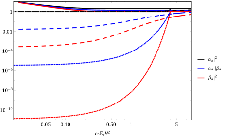
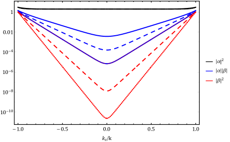
Figure 1: The left panel of the figure shows the combinations of the Bogoliubov coefficients $|\alpha_{\mathbf{k}}|^{2}$ in black, $|\alpha_{\mathbf{k}}||\beta_{\mathbf{k}}|$ in blue and $|\beta_{\mathbf{k}}|^{2}$ in red as a function of electric field by taking $k_{z}/k=1$. For the right panel, we combine the contribution of the positive charged particles and negative charged particles to the Bogoliubov coefficients. This contributes to the symmetry of the figure. The solid and dashed lines correspond to $m=3H/2$ and $2H$ respectively. The dotted line corresponds to fixing $|\mu|=4$ and hence the electric field $e_{0}E/H^{2}$ cannot exceed $4$ as $\tilde{m}=\sqrt{m^{2}-9/4}\geq 0$. The right panel of the figure shows the Bogoliubov coefficients as a function of $k_{z}/k$. The solid, dashed and dotted lines represents $\mu=2i,3i,4i$, respectively.

In the classical limit, the particle production rate is given approximately by

$$n_{\mathbf{k}} \approx e^{-S_{E}}=e^{-2\pi(|\mu|\pm|\kappa|)}=e^{-S_{\pm}}=e^{-2\pi\frac{\tilde{m}}{H}(\sqrt{1+l^{2}}\pm\frac{|k_{z}|}{k}l)}~{},$$ (16)

where $l\equiv e_{0}E/\tilde{m}H$ characterizes the relative magnitude of the electric field and mass. $\tilde{m}^{2}=m^{2}-9H^{2}/4$ is the effective mass of a neutral particle in de Sitter space. $S_{+}$ is the action corresponding to the action of the process that the charged particles are produced but moving to the direction that increases the electric potential energy of itself, whereas $S_{-}$ corresponds to the action of the process that the charged particles are produced and moving to the direction that decreases the electric potential energy. It is always the $S_{-}$ that gives the dominant contribution.

There are two interesting limits that we can discuss this problem quite intuitively. The first limit is the weak electric field limit, where $l\ll 1$. The classical actions $S_{\pm}$ in (16) can be approximated as

$$S_{\pm}=2\pi\bigg{(}\frac{\tilde{m}}{H}\pm\frac{|k_{z}|}{k}\frac{e_{0}E}{H^{2}}\bigg{)}~{}.$$ (17)

The first term can be understood as the usual Boltzman factor coming from the production of neutral massive particles of effective mass $\tilde{m}$. From the point of view of a geodesic observer, de Sitter space is associated with a thermal bath with the Hawking temperature $T=H/(2\pi)$. The second term is understood as the chemical potential from the electric field. This chemical potential can assist the production of charged particles along the direction of decreasing potential. Since in this limit, the electric field is very weak, the dominant contribution comes from the first term. Hence, although the particles are charged, they are mainly produced gravitationally due to the expansion of the universe. In Adshead:2015kza ; Adshead:2018oaa ; Chen:2018xck , other examples of the chemical potential is also discussed in the context of fermion production in inflation.

The other limit is the large electric field limit, where $l\gg 1$. In this limit, the electric field is so strong that the modes do not feel the curvature of the spacetime. The classical actions $S_{\pm}$ can be approximated as

$$S_{+}=2\pi\frac{e_{0}E}{H^{2}}\bigg{(}1+\frac{|k_{z}|}{k}\bigg{)}\quad S_{-}=2\pi\bigg{(}\frac{e_{0}E}{H^{2}}\bigg{(}1-\frac{|k_{z}|}{k}\bigg{)}+\frac{\tilde{m}^{2}}{2e_{0}E}\bigg{)}~{}.$$ (18)

If we consider the charged particle pairs moving along the $z$ direction, the second term dominates. As we can see, it also reproduces the flat spacetime result.

In order to study the time scale of mass production of charged particles, it is useful to consider the WKB approximation of solution (11).

$$av_{\mathbf{k}}=\frac{1}{\sqrt{2|w_{\mathbf{k}}|}}\exp\bigg{\{}-i\int^{\tau}d\tau|w_{\mathbf{k}}|\bigg{\}}~{},$$ (19)

where $w_{\mathbf{k}}$ is the effective frequency given by

$$w_{\mathbf{k}}^{2} =(k_{z}+e(\theta_{0})A_{z})^{2}+k_{x}^{2}+k_{y}^{2}+a^{2}m^{2}-\frac{a^{\prime\prime}}{a}$$

$$=\frac{1}{\tau^{2}}\bigg{(}\frac{e_{0}^{2}E^{2}}{H^{4}}+\frac{m^{2}}{H^{2}}-2\bigg{)}+\frac{2}{\tau}\frac{k_{z}e_{0}E}{H^{2}}+k^{2}~{},\quad k\equiv(k_{x}^{2}+k_{y}^{2}+k_{z}^{2})^{1/2}~{}.$$ (20)

Then the adiabatic parameter is evaluated as

$$\bigg{|}\frac{w^{\prime}_{\mathbf{k}}}{w_{\mathbf{k}}^{2}}\bigg{|}=\bigg{|}\frac{H^{2}(e_{0}^{2}E^{2}+e_{0}EH^{2}k_{z}\tau-2H^{4}+H^{2}m^{2})}{\left(e_{0}^{2}E^{2}+2e_{0}EH^{2}k_{z}\tau-2H^{4}+H^{2}m^{2}+k^{2}H^{4}\tau^{2}\right)^{3/2}}\bigg{|}~{}.$$ (21)

It is around the time

$$\tau\sim-\frac{1}{k}\bigg{(}|\mu|^{2}+\frac{1}{4}\bigg{)}^{1/4}~{},$$ (22)

that the quantity $w^{\prime}_{\mathbf{k}}/w_{\mathbf{k}}^{2}$ approaches its maximum. This means that most particles are produced at this time scale.

Now we observe the production of the particle via the Schwinger effect during inflation. One may think about the mechanism in the context of quasi-single field inflation. The charged particles can decay into the primordial curvature perturbations, thus leaving an imprint on the primordial power spectrum and bispectrum. $\zeta$ is the primordial curvature perturbation. The second order action of the primordial curvature perturbation can be written down following the procedure in Chen:2010xka ; Wang:2013eqj

$$S_{\zeta}=M_{p}^{2}\int dt\frac{d^{3}k}{(2\pi)^{3}}\epsilon(a^{3}\dot{\zeta}^{2}-k^{2}a\zeta^{2})~{}.$$ (23)

Quantizing it in the following way

$$\zeta_{\mathbf{k}} =u_{\mathbf{k}}c_{\mathbf{k}}+u_{\mathbf{k}}^{*}c^{\dagger}_{-\mathbf{k}}~{},$$ (24)

where $c^{\dagger}_{\mathbf{k}}$, $c_{\mathbf{k}}$ are the creation and annihilation operators satisfying the usual commutation relations

$$[c_{\mathbf{k}},c^{\dagger}_{\mathbf{p}}]=(2\pi)^{3}\delta^{(3)}(\mathbf{k}-\mathbf{p})~{}.$$ (25)

The mode function satisfies the following equation of motion

$$\ddot{\zeta}+(3+\eta)H\dot{\zeta}+\frac{k^{2}}{a^{2}}\zeta=0~{}.$$ (26)

To the lowest order in slow roll parameter, the solution is

$$u_{\mathbf{k}}(\tau)=\frac{H}{2\sqrt{\epsilon}M_{\rm pl}}\frac{1}{k^{3/2}}(1+ik\tau)e^{-ik\tau}~{}.$$ (27)

We consider the following coupling between the primordial curvature perturbation and the positive charged scalar fields

$$L_{\delta\sigma\zeta^{\prime}} =c_{2}\int d^{3}xd\tau a^{3}\delta\sigma\zeta^{\prime},\quad L_{\delta\sigma\zeta^{\prime}\zeta^{\prime}}=c_{3}\int d^{3}xd\tau a^{2}\delta\sigma\zeta^{\prime}\zeta^{\prime}~{},$$ (28)

$$c_{2} =-\frac{2R\dot{\theta}_{0}^{2}}{H},\quad c_{3}=\frac{\dot{\theta}^{2}_{0}R}{H^{2}}~{}.$$ (29)

The coupling between the inflaton and the negative charged scalar fields are

$$L_{\delta\sigma^{*}\zeta^{\prime}} =c^{*}_{2}\int d^{3}xd\tau a^{3}\delta\sigma^{*}\zeta^{\prime},\quad L_{\delta\sigma^{*}\zeta^{\prime}\zeta^{\prime}}=c_{3}^{*}\int d^{3}xd\tau a^{2}\delta\sigma^{*}\zeta^{\prime}\zeta^{\prime}~{},$$ (30)

$$c_{2}^{*} =-\frac{2R\dot{\theta}_{0}^{2}}{H},\quad c_{3}^{*}=\frac{\dot{\theta}^{2}_{0}R}{H^{2}}~{},$$ (31)

and the coupling between the primordial curvature perturbation and the positive and negative charged scalar fields are

$$L_{\delta\sigma\delta\sigma^{*}\zeta^{\prime}} =c^{\prime}_{2}\int d^{3}xd\tau a^{3}\delta\sigma\delta\sigma^{*}\zeta^{\prime},\quad L_{\delta\sigma\delta\sigma^{*}\zeta^{\prime}\zeta^{\prime}}=c^{\prime}_{3}\int d^{3}xd\tau a^{2}\delta\sigma\delta\sigma^{*}\zeta^{\prime}\zeta^{\prime}~{},$$ (32)

$$c_{2}^{\prime} =-\frac{\dot{\theta}_{0}^{2}(\sigma_{0}+R)}{H\sigma_{0}},\quad c_{3}^{\prime}=\frac{\dot{\theta}_{0}^{2}}{H^{2}}~{},$$ (33)

where $c_{2}$, $c_{3}$, $c_{2}^{*}$, $c_{3}^{*}$, $c^{\prime}_{2}$ and $c^{\prime}_{3}$ are some constants. Here we pick some of the possible interacting terms in (28), (30) and (32) (For the full analysis of the Lagrangian, please refer to Appendix B). For $c_{3}$, $c_{3}^{*}$, $c^{\prime}_{2}$ and $c^{\prime}_{3}$, we only show the leading order term involved. We can also see that (28) and (30) do not conserve the charge of $\delta\sigma$. They correspond to cases where the phase symmetry of $\delta\sigma$ is broken, for example, in an Abelian Higgs model (see Kumar:2017ecc for discussion of a similar case). In other words, the gauge invariance is broken. The breaking of U(1) gauge invariance can have some benefits. For example, the strong coupling problem and backreaction can be evaded Domenech:2015zzi , though the mechanism to obtain it is still an open problem. In this case, tree level contribution dominates correction to the spectra. Equation (32) corresponds to the case where charge is conserved. In this case, loop diagrams has to be computed. One may worry that these background values contribute to the mass of the gauge field and it won’t be able to support a long range force. But now we are considering very small coefficients. In order to calculate the primordial spectrums, we used the Schwinger-Keldysh formalism (For the application in quasi-single field inflation, see Chen:2017ryl ). Now we derive the four types of free propagators for both the curvature perturbation and the massive charged scalar fields. For the curvature perturbation sector, the generating functional can be written as

$$Z_{0}[J_{+},J_{-}]\equiv\int\mathcal{D}\mathcal{\zeta}_{+}\mathcal{D}\mathcal{\zeta}_{-}\exp\bigg{[}i\int_{\tau_{0}}^{\tau_{f}}d\tau d^{3}x\bigg{(}\mathcal{L}_{0}[\zeta_{+}]-\mathcal{L}_{0}[\zeta_{-}]+J_{+}\zeta_{+}-J_{-}\zeta_{-}\bigg{)}\bigg{]}~{}.$$ (34)

The four propagators can be generated using

$$-i\Delta_{ab}(\tau_{1},\mathbf{x}_{1};\tau_{2},\mathbf{x}_{2})=\frac{\delta}{ia\delta J_{a}(\tau_{1},\mathbf{x}_{1})}\frac{\delta}{ib\delta J_{b}(\tau_{2},\mathbf{x}_{2})}Z_{0}[J_{+},J_{-}]\bigg{|}_{J_{\pm}=0}~{},\quad a,b=\pm~{}.$$ (35)

Fourier transforming it into momentum space gives

$$G_{ab}({\mathbf{k}};\tau_{1},\tau_{2})=-\int d^{3}\mathbf{x}e^{-i\mathbf{k}\cdot\mathbf{x}}\Delta_{ab}(\tau_{1},\mathbf{x};\tau_{2},\mathbf{0})~{}.$$ (36)

The four types of propagators are given as the following

$$G_{++}({\mathbf{k}},\tau_{1},\tau_{2}) = \theta(\tau_{1}-\tau_{2})u_{\mathbf{k}}(\tau_{1})u_{\mathbf{k}}^{*}(\tau_{2})+\theta(\tau_{2}-\tau_{1})u_{\mathbf{k}}^{*}(\tau_{1})u_{\mathbf{k}}(\tau_{2})$$

$$G_{+-}({\mathbf{k}},\tau_{1},\tau_{2}) = u_{\mathbf{k}}^{*}(\tau_{1})u_{\mathbf{k}}(\tau_{2})$$

$$G_{-+}({\mathbf{k}},\tau_{1},\tau_{2}) = u_{\mathbf{k}}(\tau_{1})u_{\mathbf{k}}^{*}(\tau_{2})$$

$$G_{--}({\mathbf{k}},\tau_{1},\tau_{2}) = \theta(\tau_{1}-\tau_{2})u_{\mathbf{k}}^{*}(\tau_{1})u_{\mathbf{k}}(\tau_{2})+\theta(\tau_{2}-\tau_{1})u_{\mathbf{k}}(\tau_{1})u_{\mathbf{k}}^{*}(\tau_{2})~{}.$$ (37)

For charged massive scalar pairs, we need to introduce two more sources $J^{*}_{+}$ and $J^{*}_{-}$ to source the complex conjugate of the $\sigma$ field

$$Z_{0}[J_{+},J_{-},J^{*}_{+},J^{*}_{-}]$$

$$\equiv\int\mathcal{D}\delta\sigma_{+}\mathcal{D}\delta\sigma_{-}\mathcal{D}\delta\sigma^{*}_{+}\mathcal{D}\delta\sigma^{*}_{-}\exp\bigg{[}i\int_{\tau_{0}}^{\tau_{f}}d\tau d^{3}x\bigg{(}\mathcal{L}_{0}[\delta\sigma_{+},\delta\sigma^{*}_{+}]-\mathcal{L}_{0}[\delta\sigma_{-},\delta\sigma_{-}^{*}]+J_{+}\delta\sigma_{+}-J_{-}\delta\sigma_{-}+J^{*}_{+}\delta\sigma^{*}_{+}-J^{*}_{-}\delta\sigma^{*}_{-}\bigg{)}\bigg{]}~{}.$$ (38)

The four propagators can be generated using

$$-i\Delta_{ab}(\tau_{1},\mathbf{x}_{1};\tau_{2},\mathbf{x}_{2})=\frac{\delta}{ia\delta J_{a}(\tau_{1},\mathbf{x}_{1})}\frac{\delta}{ib\delta J^{*}_{b}(\tau_{2},\mathbf{x}_{2})}Z_{0}[J_{+},J_{-},J^{*}_{+},J^{*}_{-}]\bigg{|}_{J_{\pm}=0,J^{*}_{\pm}=0}~{},\quad a,b=\pm~{}.$$ (39)

Then we have

$$\begin{pmatrix}D_{++}(\mathbf{k},\tau;\mathbf{k}^{\prime},\tau^{\prime})&D_{+-}(\mathbf{k},\tau;\mathbf{k}^{\prime},\tau^{\prime})\\ D_{-+}(\mathbf{k},\tau;\mathbf{k}^{\prime},\tau^{\prime})&D_{--}(\mathbf{k},\tau;\mathbf{k}^{\prime},\tau^{\prime})\end{pmatrix}=i\begin{pmatrix}\langle T\delta\sigma_{\mathbf{k}}(\tau)\delta\sigma^{*}_{\mathbf{k}^{\prime}}(\tau^{\prime})\rangle&\langle\delta\sigma^{*}_{\mathbf{k}}(\tau)\delta\sigma_{\mathbf{k}^{\prime}}(\tau^{\prime})\rangle\\ \langle\delta\sigma_{\mathbf{k}}(\tau)\delta\sigma^{*}_{\mathbf{k}^{\prime}}(\tau^{\prime})\rangle&\langle\bar{T}\delta\sigma^{*}_{\mathbf{k}}(\tau)\delta\sigma_{\mathbf{k}^{\prime}}(\tau^{\prime})\rangle\end{pmatrix}~{}.$$ (40)

The four types of propagators in the Schwinger-Keldysh formalism are

$$D_{++}({\mathbf{k}},\tau_{1},\tau_{2}) = \theta(\tau_{1}-\tau_{2})v_{\mathbf{k}}(\tau_{1})v_{\mathbf{k}}^{*}(\tau_{2})+\theta(\tau_{2}-\tau_{1})v_{\mathbf{k}}^{*}(\tau_{1})v_{\mathbf{k}}(\tau_{2})$$

$$D_{+-}({\mathbf{k}},\tau_{1},\tau_{2}) = v_{\mathbf{k}}^{*}(\tau_{1})v_{\mathbf{k}}(\tau_{2})$$

$$D_{-+}({\mathbf{k}},\tau_{1},\tau_{2}) = v_{\mathbf{k}}(\tau_{1})v_{\mathbf{k}}^{*}(\tau_{2})$$

$$D_{--}({\mathbf{k}},\tau_{1},\tau_{2}) = \theta(\tau_{1}-\tau_{2})v_{\mathbf{k}}^{*}(\tau_{1})v_{\mathbf{k}}(\tau_{2})+\theta(\tau_{2}-\tau_{1})v_{\mathbf{k}}(\tau_{1})v_{\mathbf{k}}^{*}(\tau_{2})~{}.$$ (41)

III The Geodesic Equation

To understand the charged particles motion in inflation, we solve the geodesic equation as an intuitive understanding. Following from our metric in (2), the following geodesic equation for a massive charged particle can be written down following the standard procedure (see text books WeinbergGravitationandCosmology ; Carroll:2004st ).

$$\frac{d^{2}x^{\mu}}{ds^{2}}=-\Gamma^{\mu}_{\alpha\beta}\frac{dx^{\alpha}}{ds}\frac{dx^{\beta}}{ds}+\frac{e(\theta_{0})}{m}F^{\mu\beta}\frac{dx^{\alpha}}{ds}g_{\alpha\beta},\quad g_{\alpha\beta}\frac{dx^{\alpha}}{ds}\frac{dx^{\beta}}{ds}=-1~{},$$ (42)

where the connection is

$$\Gamma^{\lambda}_{\alpha\beta}=\frac{1}{2}g^{\lambda\tau}\bigg{(}\frac{\partial g_{\tau\alpha}}{dx^{\beta}}+\frac{\partial g_{\tau\beta}}{\partial x^{\alpha}}-\frac{\partial g_{\alpha\beta}}{\partial x^{\tau}}\bigg{)}~{}.$$ (43)

Here, we would like to observe the change in the physical velocity of the massive charged particle. We would like to solve the following geodesic equation:

$$\frac{d^{2}x(t)}{dt^{2}}=-2\frac{\dot{a}}{a}\frac{dx(t)}{dt}+\frac{e_{0}}{m}a^{-1}E~{}.$$ (44)

The initial condition we would choose is $\dot{x}(t_{0})=0$, which means that the particles are produced at zero velocity. The solution to this equation subjected to the initial condition is

$$x(t)=\frac{Ee_{0}}{mH^{2}}e^{-Ht}\bigg{(}\text{cosh}(H(t-t_{0}))-1\bigg{)}~{}.$$ (45)

The velocity of the particle is

$$\dot{x}(t)=\frac{Ee_{0}}{mH}\bigg{(}e^{-Ht}-e^{Ht_{0}-2Ht}\bigg{)}~{}.$$ (46)

At first, the force from electric field dominates over the Hubble friction and the particle starts to accelerate. Later, the particle decelerates due to the Hubble friction. The maximum velocity occurs in the subhorizon.

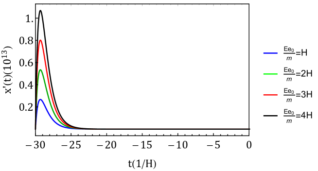
Figure 2: The comoving velocity of the particle with respect to the physical time $t$. We take the Hubble parameter to be $1$ in making the plot. We choose the initial time to be $t_{0}=-30$ and $t_{f}=30$ to ensure 60 e-folds. We here plot the evolution of the velocity in the subhorizon level. Initially, the velocity of the particle is zero. Through the acceleration from the electric field, the velocity of the particle increases and the direction depends on the charge of the particle. For stronger electric fields,the maximum velocity attained is much larger. After some time, the particle starts to decelerate and its velocity slowly decreases to zero due to the Hubble expansion of the universe. We can see the velocity has decreased to zero at subhorizon level. Hence, the change in the frequency of the oscillatory signal in the bispectrum can’t be observed as the bispectrum is imprinted at late times.

IV Power Spectrum

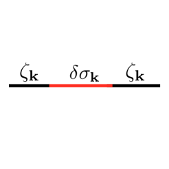
Figure 3: The Feynman diagram we are considering for the correction to the power spectrum. This diagram involves the interaction of $\delta\sigma$ with the inflaton. For the total correction, we need to include the correction from $\delta\sigma^{*}$.

In this section, we study the correction to the power spectrum of our model, which can be shown in FIG. 3. It can be evaluated using the Schwinger-Keldysh formalism Chen:2017ryl

$$\langle\zeta_{\mathbf{k}}\zeta_{-\mathbf{k}}\rangle^{\prime}=|c_{2}|^{2}\sum_{a,b=\pm}ab\int_{-\infty}^{0}\int_{-\infty}^{0}\frac{d\tau_{1}}{(-H\tau_{1})^{3}}\frac{d\tau_{2}}{(-H\tau_{2})^{3}} \partial_{\tau_{1}}G_{a+}({\mathbf{k}},\tau_{1},0)D_{ab}({\mathbf{k}},\tau_{1},\tau_{2})\partial_{\tau_{2}}G_{b+}({\mathbf{k}},\tau_{2},0)+({\kappa\rightarrow-\kappa})~{},$$ (47)

where $G(\mathbf{k},\tau_{1},\tau_{2})$ and $D(\mathbf{k},\tau_{1},\tau_{2})$ are defined by (II) and (II) respectively. Here, we need to do a sum over of all the $+$ and $-$ modes. The ^′ means the momentum conserving delta function $(2\pi)^{3}\delta^{(3)}(\mathbf{k}+\mathbf{k}^{\prime})$ is stripped from the two point function.

There are two contributions, the first is

$$\langle\zeta_{\mathbf{k}}\zeta_{-\mathbf{k}}\rangle^{\prime(1)}=2|c_{2}|^{2}\frac{e^{i\pi\kappa}}{32k^{3}M_{\rm pl}^{4}\epsilon^{2}}\bigg{|}\int_{0}^{\infty}dx_{1}\frac{e^{ix_{1}}W_{\kappa,\mu}(-2ix_{1})}{x_{1}}\bigg{|}^{2}+(\kappa\rightarrow-\kappa)~{}.$$ (48)

The indefinite integral can be integrated directly, which yields

$$\mathcal{I}=\int dx\frac{e^{ix}W_{\kappa,\mu}(-2ix)}{x}=G_{2,3}^{2,1}\left(-2ix\left|\begin{array}[]{c}1,-\kappa+1\\ \frac{1}{2}-\mu,\mu+\frac{1}{2},0\\ \end{array}\right.\right)~{},$$ (51)

where $G$ is the Meijer function defined through the Gamma function in the following way

$$G_{p,q}^{m,n}\left(x\left|\begin{array}[]{c}a_{1},\ldots,a_{p}\\ b_{1},\ldots,b_{q}\\ \end{array}\right.\right)\equiv\frac{1}{2\pi i}\int_{\gamma_{L}}\frac{\prod_{j=1}^{m}\Gamma(b_{j}-s)\prod^{n}_{j=1}\Gamma(1-a_{j}+s)}{\prod_{j=n+1}^{p}\Gamma(a_{j}-s)\prod^{q}_{j=m+1}\Gamma(1-b_{j}+s)}x^{s}ds~{}.$$ (54)

At $x=0$, the integral $\mathcal{I}$ gives $0$. At $x\rightarrow\infty$, it gives

$$\frac{\Gamma(\frac{1}{2}-\mu)\Gamma(\frac{1}{2}+\mu)}{\Gamma(1-\kappa)}~{}.$$ (55)

The second contributions is

$$\langle\zeta_{\mathbf{k}}\zeta_{-\mathbf{k}}\rangle^{\prime(2)}=-4|c_{2}|^{2}\frac{e^{i\pi\kappa}}{32k^{3}M_{\rm pl}^{4}\epsilon^{2}}{\rm Re}\bigg{[}\int_{0}^{\infty}dx_{2}\frac{e^{-ix_{2}}W_{-\kappa,-\mu}(2ix_{2})}{x_{2}}\int_{0}^{x_{2}}dx_{1}\frac{e^{-ix_{1}}W_{\kappa,\mu}(-2ix_{1})}{x_{1}}\bigg{]}+(\kappa\rightarrow-\kappa)~{}.$$ (56)

This integral is difficult to evaluate, thus, we use series expansion to calculate the analytical expression for the integral. The detailed calculation of the power spectrum is presented in Appendix D

$$\langle\zeta_{\mathbf{k}}\zeta_{-\mathbf{k}}\rangle^{\prime(2)}=-4|c_{2}|^{2}\frac{e^{i\pi\kappa}}{32k^{3}M_{\rm pl}^{4}\epsilon^{2}}{\rm Re}[\mathcal{I}_{2}]+(\kappa\rightarrow-\kappa)~{},$$ (57)

where $\mathcal{I}_{2}=P_{1}+P_{2}+P_{3}+P_{4}$. We present the expression of each component explicitly

$$P_{1} =\frac{\Gamma(2\mu)\Gamma(-2\mu)}{\Gamma(\frac{1}{2}+\mu+\kappa)\Gamma(\frac{1}{2}-\mu-\kappa)}\sum_{n=0}^{\infty}\sum_{m=0}^{\infty}\frac{(-1)^{\frac{1}{2}+\mu+n+2m}2}{n!m!(\frac{1}{2}+\mu+m)}\Gamma(1+m+n)$$ (58)

$$\,{}_{2}F_{1}\left(-n,-\mu+\kappa+\frac{1}{2};1-2\mu;2\right)\,_{2}F_{1}\left(-m,\mu-\kappa+\frac{1}{2};2\mu+1;2\right)\,_{2}F_{1}\left(1+m+n,\frac{1}{2}+\mu+m;\frac{3}{2}+\mu+m;-1\right)~{},$$

$$P_{2} =\frac{\Gamma(2\mu)\Gamma(2\mu)}{\Gamma(\frac{1}{2}+\mu+\kappa)\Gamma(\mu-\kappa+\frac{1}{2})}\sum_{n=0}^{\infty}\sum_{m=0}^{\infty}\frac{(-1)^{\frac{1}{2}-\mu+n+2m}2^{1-2\mu}}{n!m!(\frac{1}{2}-\mu+m)}\Gamma(1-2\mu+m+n)$$ (59)

$$\,{}_{2}F_{1}\left(-n,-\mu+\kappa+\frac{1}{2};1-2\mu;2\right)\,_{2}F_{1}\left(-m,-\mu-\kappa+\frac{1}{2};2\mu+1;2\right)\,_{2}F_{1}\left(1-2\mu+m+n,\frac{1}{2}-\mu+m;\frac{3}{2}-\mu+m;-1\right)~{},$$

$$P_{3} =\frac{\Gamma(-2\mu)\Gamma(-2\mu)}{\Gamma(-\mu+\kappa+\frac{1}{2})\Gamma(\frac{1}{2}-\mu-\kappa)}\sum_{n=0}^{\infty}\sum_{m=0}^{\infty}\frac{(-1)^{\frac{1}{2}+\mu+n+2m}2^{1+2\mu}}{n!m!(\frac{1}{2}+\mu+m)}\Gamma(1+2\mu+m+n)$$ (60)

$$\,{}_{2}F_{1}\left(-n,\mu+\kappa+\frac{1}{2};1-2\mu;2\right)\,_{2}F_{1}\left(-m,\mu-\kappa+\frac{1}{2};2\mu+1;2\right)\,_{2}F_{1}\left(1+2\mu+m+n,\frac{1}{2}+\mu+m;\frac{3}{2}+\mu+m;-1\right)~{},$$

$$P_{4} =\frac{\Gamma(-2\mu)\Gamma(2\mu)}{\Gamma(-\mu+\kappa+\frac{1}{2})\Gamma(\mu-\kappa+\frac{1}{2})}\sum_{n=0}^{\infty}\sum_{m=0}^{\infty}\frac{(-1)^{\frac{1}{2}-\mu+n+2m}2}{n!m!(\frac{1}{2}-\mu+m)}\Gamma(1+m+n)$$ (61)

$$\,{}_{2}F_{1}\left(-n,\mu+\kappa+\frac{1}{2};1-2\mu;2\right)\,_{2}F_{1}\left(-m,-\mu-\kappa+\frac{1}{2};2\mu+1;2\right)\,_{2}F_{1}\left(1+m+n,\frac{1}{2}-\mu+m;\frac{3}{2}-\mu+m;-1\right)~{}.$$

We can see that $m=0,n=0$ of $P_{1}$ contributes to the leading order term of $\mathcal{I}_{2}$ in FIG.13. We then would apply this approximation in calculating $\mathcal{I}_{2}$,

$$\mathcal{I}_{2} \approx\frac{\Gamma(2\mu)\Gamma(-2\mu)}{\Gamma(\frac{1}{2}+\mu+\kappa)\Gamma(\frac{1}{2}-\mu-\kappa)}\frac{(-1)^{\frac{1}{2}+\mu}2}{(\frac{1}{2}+\mu)}$$ (62)

$$\,{}_{2}F_{1}\left(0,-\mu+\kappa+\frac{1}{2};1-2\mu;2\right)\,_{2}F_{1}\left(0,\mu-\kappa+\frac{1}{2};2\mu+1;2\right)\,_{2}F_{1}\left(1,\frac{1}{2}+\mu;\frac{3}{2}+\mu;-1\right)$$

$$=\frac{ie^{-i\pi\mu}}{2\mu}\csc(2\pi\mu)\cos(\pi(\kappa+\mu))\left(\psi^{(0)}\left(\frac{\mu}{2}+\frac{1}{4}\right)-\psi^{(0)}\left(\frac{\mu}{2}+\frac{3}{4}\right)\right)~{}.$$

The power spectrum $P_{\zeta}$ is obtained as

$$\langle\zeta_{\mathbf{k}}\zeta_{-\mathbf{k}}\rangle^{\prime}=\langle\zeta_{\mathbf{k}}\zeta_{-\mathbf{k}}\rangle^{\prime(1)}+\langle\zeta_{\mathbf{k}}\zeta_{-\mathbf{k}}\rangle^{\prime(2)}\equiv\frac{2\pi^{2}}{k^{3}}P_{\zeta}(\mathbf{k})~{}.$$ (63)

From here and the following, when making the plot, we set $c_{2}=c_{3}=M_{\rm pl}=\epsilon=H=1$. We plot the angular dependence of the power spectrum in FIG. 4. The produced charged particles can leave non trivial angular dependence on the power spectrum. The power spectrum grows exponentially as the quantity $k_{z}/k$ increases. This signature is understood as the production of virtual particles increases exponentially when the momentum of the positive charged massive scalar particle is aligned with the electric field $E$ whereas the momentum of the negative charged massive scalar particle is opposite to the direction of the electric field $E$. This signature is a unique signature which cannot be generated by other mechanisms to the knowledge we know of.

We also plot the dependence of the power spectrum on electric field strength in FIG. 5 and the dependence of the power spectrum on the mass of massive field in FIG. 6.

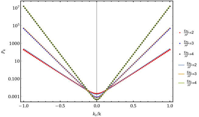
Figure 4: We here make a comparison on the analytical (line plot) and numerical (dotted plot) results for different electric field strength. At different electric field strength, the power spectrum has different angular dependence. We set the mass of massive field to be $3H/2$. When the orientation is aligned to the orientation of the field, the power spectrum is much larger. If the orientation is perpendicular to the orientation of the field, although the electric field is strong, Schwinger effect is weak and the effective mass is large enough to suppress the power spectrum, hence, the power spectrum can be small with strong electric field strength. At the orientation parallel to the field’s orientation, the Schwinger effect is strong enough to get a large power spectrum.

Figure 5: We set $k_{z}/k=1$ and the mass of the massive field to be $3H/2,9H/2,15H/2,21H/2,27H/2,33H/2,39H/2$ respectively. The power spectrum increases exponentially with respect to the electric field strength.

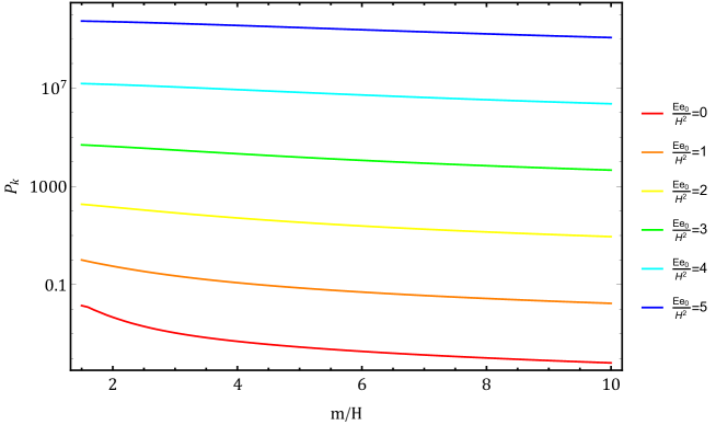
Figure 6: We set $k_{z}/k=1$ and $\kappa=0,-i,-2i,-3i,-4i,-5i,-6i$ respectively. For small electric field strength, the power spectrum decreases following the power $1/|\mu|^{2}$, whereas when the electric field strength increases, the power spectrum decays exponentially when the mass increases.

V Bispectrum

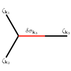
Figure 7: The Feynman diagram of the bispectrum that involves the interaction of $\delta\sigma$ with the inflaton. For the total contribution, we need to include the correction from $\delta\sigma^{*}$.

In this section, we study the bispectrum of this model, which is shown in FIG. 7. For the bispectrum, using the Schwinger-Keldysh formalism Chen:2017ryl , the bispectrum can be expressed as

$$\langle\zeta_{\mathbf{k}_{1}}\zeta_{\mathbf{k}_{2}}\zeta_{\mathbf{k}_{3}}\rangle^{\prime} =c_{2}c^{*}_{3}\sum_{a,b=\pm}ab\int_{-\infty}^{0}\int_{-\infty}^{0}\frac{d\tau_{1}}{(-H\tau_{1})^{3}}\frac{d\tau_{2}}{(-H\tau_{2})^{2}}\partial_{\tau_{1}}G_{a+}({\mathbf{k}_{3}},\tau_{1},0)D_{ab}({\mathbf{k}_{3}},\tau_{1},\tau_{2})\partial_{\tau_{2}}G_{b+}({\mathbf{k}_{1}},\tau_{2},0)\partial_{\tau_{2}}G_{b+}({\mathbf{k}_{2}},\tau_{2},0)$$

$$+({\kappa\rightarrow-\kappa},c_{2}\rightarrow c_{2}^{*},c_{3}^{*}\rightarrow c_{3})~{}.$$ (64)

There are three contributions

$$\langle\zeta_{\mathbf{k}_{1}}\zeta_{\mathbf{k}_{2}}\zeta_{\mathbf{k}_{3}}\rangle^{\prime}=\langle\zeta_{\mathbf{k}_{1}}\zeta_{\mathbf{k}_{2}}\zeta_{\mathbf{k}_{3}}\rangle^{\prime(1)}+\langle\zeta_{\mathbf{k}_{1}}\zeta_{\mathbf{k}_{2}}\zeta_{\mathbf{k}_{3}}\rangle^{\prime(2)}+\langle\zeta_{\mathbf{k}_{1}}\zeta_{\mathbf{k}_{2}}\zeta_{\mathbf{k}_{3}}\rangle^{\prime(3)}+{\rm 5\,\,Permutations}+({\kappa\rightarrow-\kappa},c_{2}\rightarrow c_{2}^{*},c_{3}^{*}\rightarrow c_{3})~{},$$ (65)

where $\langle\zeta_{\mathbf{k}_{1}}\zeta_{\mathbf{k}_{2}}\zeta_{\mathbf{k}_{3}}\rangle^{\prime(1)}$, $\langle\zeta_{\mathbf{k}_{1}}\zeta_{\mathbf{k}_{2}}\zeta_{\mathbf{k}_{3}}\rangle^{\prime(2)}$ and $\langle\zeta_{\mathbf{k}_{1}}\zeta_{\mathbf{k}_{2}}\zeta_{\mathbf{k}_{3}}\rangle^{\prime(3)}$ are computed as

$$\langle\zeta_{\mathbf{k}_{1}}\zeta_{\mathbf{k}_{2}}\zeta_{\mathbf{k}_{3}}\rangle^{\prime(1)}=-2c_{2}c^{*}_{3}\frac{H^{3}e^{i\pi\kappa}}{128\epsilon^{3}k_{1}k_{2}k^{4}_{3}M_{\rm pl}^{6}}\int_{0}^{\infty}dx_{1}\frac{e^{ix_{1}}W_{\kappa,\mu}(-2ix_{1})}{x_{1}}\int_{0}^{\infty}dx_{2}x_{2}e^{-i\frac{k_{1}+k_{2}}{k_{3}}x_{2}}W_{-\kappa,-\mu}(2ix_{2})~{}.$$

$$\langle\zeta_{\mathbf{k}_{1}}\zeta_{\mathbf{k}_{2}}\zeta_{\mathbf{k}_{3}}\rangle^{\prime(2)}=2c_{2}c^{*}_{3}\frac{H^{3}e^{i\pi\kappa}}{128\epsilon^{3}k_{1}k_{2}k^{4}_{3}M_{\rm pl}^{6}}{\rm Re}\bigg{[}\int_{0}^{\infty}dx_{2}x_{2}e^{-i\frac{k_{1}+k_{2}}{k_{3}}x_{2}}W_{-\kappa,-\mu}(2ix_{2})\int_{0}^{x_{2}}dx_{1}\frac{e^{-ix_{1}}W_{\kappa,\mu}(-2ix_{1})}{x_{1}}\bigg{]}~{}.$$

$$\langle\zeta_{\mathbf{k}_{1}}\zeta_{\mathbf{k}_{2}}\zeta_{\mathbf{k}_{3}}\rangle^{\prime(3)}=2c_{2}c^{*}_{3}\frac{H^{3}e^{i\pi\kappa}}{128\epsilon^{3}k_{1}k_{2}k^{4}_{3}M_{\rm pl}^{6}}{\rm Re}\bigg{[}\int_{0}^{\infty}dx_{2}\frac{e^{-ix_{2}}W_{-\kappa,-\mu}(2ix_{2})}{x_{2}}\int_{0}^{x_{2}}dx_{1}x_{1}e^{-i\frac{k_{1}+k_{2}}{k_{3}}x_{1}}W_{\kappa,\mu}(-2ix_{1})\bigg{]}~{}.$$

Figure 8: This figure shows how we measure the non-Gaussianity. The $z$ direction denotes the direction of the electric field. When we measure the non-Gaussianity, we should fix the ratio of the long wavelength momentum and the short wavelength momentum $k_{1}/k_{3}$. In the meanwhile, we measure the angular dependence of the non-Gaussianity for different $k_{3z}/k_{3}$. $k_{3z}$ is the magnitude of the long wavelength momentum projected onto the $z$ direction.

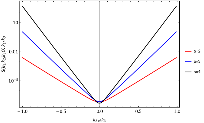
Figure 9: This figure shows the amplified shape function $S(k_{1},k_{2},k_{3})\times k_{1}/k_{3}$ as a function of the angular dependence of the soft momentum $k_{3z}/k_{3}$. In this figure, we set $m=3H/2$ and $k_{1}/k_{3}=100$. When the orientation is aligned to the orientation of the field, the amplitude of the bispectrum is much larger. At the orientation perpendicular to the field’s orientation, although the electric field strength is strong, Schwinger effect is weak and the effective mass is large enough to suppress the bispectrum. At the orientation parallel to the orientation of the field, the Schwinger effect is strong enough to generate a bispectrum of large amplitude.

We can define the bispectrum in the form of dimensionless shape function $S(k_{1},k_{2},k_{3})$ Chen:2018xck , defined as,

$$\langle\zeta_{\mathbf{k}_{1}}\zeta_{\mathbf{k}_{2}}\zeta_{\mathbf{k}_{3}}\rangle^{\prime}\equiv(2\pi)^{4}S(k_{1},k_{2},k_{3})\frac{1}{(k_{1}k_{2}k_{3})^{2}}P^{(0)2}_{\zeta}~{},$$ (66)

where $P^{(0)}_{\zeta}=\frac{1}{8\pi^{2}{M_{\rm pl}^{2}}}\frac{H^{2}}{\epsilon}$ is the power spectrum for the curvature perturbation without the correction coming from massive fields.

The bispectrum can be evaluated using numerical integration. We plot the angular dependence of the amplified bispectrum shape function $(k_{1}/k_{3})\times S(k_{1},k_{2},k_{3})$ as a function of $k_{3z}/k_{3}$ in FIG. 9. The bispectrum increases exponentially with increasing absolute value of $k_{3z}/k_{3}$. When $k_{3z}/k_{3}$ is positive, the main contribution comes from the positive charged particles whereas when $k_{3z}/k_{3}$ is negative, the main contribution comes from the negative charged particles.

We plot the clock signals of the squeeze limit of the bispectrum with fixed effective mass $\mu$ in FIG. 10 and with fixed mass $m$ in FIG. 11. In both cases, we see that the clock signal is less obvious when the strength of the electric field increases. In the case of fixing the effective mass $\mu$ case, the absolute value of the clock signal increases with increasing electric field strength due to the enhanced particle production rate. However, the relative amplitude between the clock signal and the contribution of the non-oscillating part coming from some local process decreases. This is because the contribution of the non-oscillating part increases faster than the clock signal when the electric field strength increases. For the fixed mass $m$ case, when the electric field strength increases, the amplitude of the clock signal relative to the non-oscillating part decreases more dramatically compared with the fixed effective mass case. This is because the electric field strength contributes to the effective mass of the charged massive scalar particles. The energy needed to produce a particle increases accordingly. The combination of these two effect causes the amplitude of the clock signal relative to the non-oscillating part barely observable starting from $\kappa=4i$.

Figure 10: The figure shows the clock signal from the bispectrum. Here we set the momentum to be in the z-direction and hence we set $k_{3z}/k_{3}=1$. We can see the suppression of the clock signal as the electric field increases. The frequency of the clock signal remains unchanged as the change in velocity of the produced particles occurs in the subhorizon and remains stationary during horizon crossing. Hence, no change in frequency of the oscillatory signal would be seen. However, the amplitude of the oscillatory signal would increase as the magnitude of the electric field strength increase.

Figure 11: The figure shows the clock signal from the bispectrum for $m=4H^{2}$. Here we set $k_{3z}/k_{3}=1$ again. We can see the suppression of the clock signal as the electric field increases.

The analytical expression of the clock signal in the large mass and small electric field strength can be obtained in Appendix E. We are particularly interested in the squeezed limit where $k_{1}\sim k_{2}\gg k_{3}$. In this limit, the shape function is

$$S(k_{1},k_{3})=\frac{1}{HM_{\rm pl}^{2}\epsilon}{\rm Re}\bigg{[}2^{\mu-9/2}c_{2}c_{3}^{*}f(\mu,\kappa)\bigg{(}\frac{k_{1}}{k_{3}}\bigg{)}^{-1/2-\mu}\bigg{]}+(\kappa\rightarrow-\kappa,c_{2}\rightarrow c_{2}^{*},c_{3}^{*}\rightarrow c_{3})~{},$$ (67)

with the prefactor given by

$$f(\mu,\kappa)\equiv e^{i\pi\kappa}\frac{\Gamma(-2\mu)^{2}\Gamma\left(\frac{1}{2}+\mu\right)\Gamma\left(\frac{5}{2}+\mu\right)}{\Gamma(\frac{1}{2}-\mu-\kappa)\Gamma(\frac{1}{2}+\mu-\kappa)}(1+\text{sin}\left(\pi\mu\right))~{},$$ (68)

where the full derivation can be obtained in Appendix F. We can see that in the large mass limit, all the $\Gamma$ functions contribute a factor of $e^{-2\pi|\mu|}$ and sin($\pi\mu$) would give a contribution of $e^{\pi|\mu|}$. Hence, the Boltzmann suppression factor $e^{-\pi|\mu|}$ is recovered in this limit. At the end of this section, we would like to compare several mechanisms that can generate large clock signals even if the mass of the $\sigma$ field are large. There are a few categories of mechanisms listed as the following.

• The presence of a new scale. In Flauger:2016idt , non-adiabatic production of very heavy fields is studied. The signatures of this model can be large due to the existence of another scale $\dot{\phi}$ with $\phi$ as the inflaton.

• Finite temperature effect. In Tong:2018tqf , the clock signal of the quasi-single field inflation is studied in the context of warm inflation. The particle production rate can be unsuppressed when the effective mass of the particle is changed due to the finite temperature effect.

• The presence of chemical potential. In Adshead:2015kza ; Adshead:2018oaa ; Chen:2018xck , the effect of the chemical potential is studied. The chemical potential can assist the production of the massive particles during inflation thus leaving a less suppressed clock signal. The mechanism we studied here also belongs to this category. However, our studies shows that although it is promising to generate a larger clock signal, one may worry that the contribution from the non-oscillating part will also increase.

• Non-trivial sound speed. The non-trivial sound speed of the massive field is studied in Chen:2018sce . The magnitude of the clock signal can also be larger than expected when the ratio of sound speed of the massive field and the inflaton is less than one. In Noumi:2012vr ; Lee:2016vti , the non-trivial sound speed of the inflaton is studied. It is shown in Lee:2016vti that when the sound speed of the inflaton is close to zero, there will also be a change in the suppression factor of the clock signal.

VI Loop Correction to Bispectrum

In this section, we investigate loop corrections coming from the extra massive fields to the primordial non-Gaussianities. The technique of dealing loop correction in quasi-single field inflation can be found in Arkani-Hamed:2015bza ; Chen:2016nrs ; Chen:2016uwp ; Chen:2016hrz ; Wu:2017lnh . The non-oscillatory part of the diagram is usually UV divergent and we need a systematic way of regularization and renormalization following Weinberg:2005vy ; Senatore:2009cf ; Senatore:2012nq ; Pimentel:2012tw ; Dimastrogiovanni:2018uqy . Luckily, the clock signal is free from UV divergence and we can evaluate it easily.

Using the Schwinger-Keldysh formalism, the bispectrum corresponding FIG. 12 can be obtained as

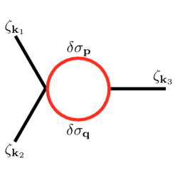
Figure 12: The Feynman diagram we are considering for the loop correction to the bispectrum.

$$\langle\zeta_{\mathbf{k}_{1}}\zeta_{\mathbf{k}_{2}}\zeta_{\mathbf{k}_{3}}\rangle^{\prime} =c^{\prime}_{2}c^{\prime}_{3}\sum_{a,b=\pm}ab\int_{-\infty}^{0}\int_{-\infty}^{0}\frac{d\tau_{1}}{(-H\tau_{1})^{3}}\frac{d\tau_{2}}{(-H\tau_{2})^{2}}\partial_{\tau_{1}}G_{a+}({\mathbf{k}_{3}},\tau_{1},0)\int\frac{d^{3}\mathbf{q}}{(2\pi)^{3}}D_{ab}(\mathbf{p},\tau_{1},\tau_{2})D_{ba}(\mathbf{q},\tau_{2},\tau_{1})$$

$$\quad\partial_{\tau_{2}}G_{b+}({\mathbf{k}_{1}},\tau_{2},0)\partial_{\tau_{2}}G_{b+}({\mathbf{k}_{2}},\tau_{2},0)+({\kappa\rightarrow-\kappa})~{},$$ (69)

where $\mathbf{p}$ and $\mathbf{q}$ are the loop momentum that satisfies the constraint $\mathbf{p}+\mathbf{q}=\mathbf{k}_{3}$. After evaluation, we get

$$\langle\zeta_{\mathbf{k}_{1}}\zeta_{\mathbf{k}_{2}}\zeta_{\mathbf{k}_{3}}\rangle^{\prime}=c^{\prime}_{2}c^{\prime}_{3}{\rm Re}\bigg{[}g(\mu,\kappa)\frac{2^{-1-8\mu}H^{5}}{k_{1}k_{2}k^{4}_{12}M_{\rm pl}^{6}\epsilon^{3}}\bigg{(}\frac{k_{12}}{k_{3}}\bigg{)}^{2\mu}\bigg{]}+({\kappa\rightarrow-\kappa})~{},$$

with the prefactor given by

$$g(\mu,\kappa)=e^{2i\pi\kappa}\frac{\Gamma(2-2\mu)\Gamma(4-2\mu)\Gamma(-2\mu)^{4}}{\Gamma(1/2-\mu-\kappa)^{2}\Gamma(1/2+\mu-\kappa)^{2}}(\text{sin}(\pi\mu))^{2}~{},$$ (70)

and with the definition of the shape function $S(k_{1},k_{2},k_{3})$ in (66) and taking the limit $k_{1}=k_{2}\gg k_{3}$, we can obtain the expression for the shape function

$$S(k_{1},k_{1},k_{3})=c^{\prime}_{2}c^{\prime}_{3}{\rm Re}\bigg{[}g(\mu,\kappa)\frac{2^{3-8\mu}H}{M_{\rm pl}^{2}\epsilon}\bigg{(}\frac{2k_{1}}{k_{3}}\bigg{)}^{2\mu-2}\bigg{]}+({\kappa\rightarrow-\kappa})~{}.$$ (71)

We can see that from the loop diagram, the massless curvature modes resonates with two pairs of massive fields and generate two sets of clock signals. The final clock signal would be contributed from the interference of these two clock signals and hence has a frequency doubled of the tree level diagram. The total Boltzmann suppression factor is of $e^{-2\pi\mu}$ where all the $\Gamma$ functions contribute $e^{-4\pi\mu}$ in total and the sin functions contribute a factor of $e^{2\pi\mu}$. The suppression for the loop correction is the square of the tree-level case due to the excitation of the two massive fields in the loop diagram.

VII Conclusion and Outlook

In this work, we consider the imprints of the Schwinger effect on the primordial power spectrum and bispectrum. Both the power spectrum and bispectrum obtained an angular dependence due to the fact that the electric field can assist the production of charged massive particles by adding a chemical potential to them. This angular dependence differs from other models that can too cause an angular dependence on the primoridial power spectrum and bispectrum. As a result, the production rate aligned or opposite to the direction of the charged particles gets enhanced. On the other hand, the production rate perpendicular to the direction of the electric field is suppresed due to the contribution of the electric field strength to the effective mass of the charged scalar particles.

There are many interesting possibilities to explore. We list a few of them and hope to address some of these possibilities in the future.

• The influence of the primordial magnetic field on the power spectrum and bispectrum in the context of quasi-single field inflation. The pair production of the charged scalar field in the presence of a constant electric and magnetic field is studied in Bavarsad:2017oyv . We would like to couple the charged particles with the inflaton and see what kind of signature these particles would imprint on the primordial power spectrum and bispectrum of the curvature perturbations. These signatures on the power spectrum and bispectrum will provide supporting evidences to the existence of the primordial magnetic field.

• The signature from other fields produced by Schwinger effect during inflation. Schwinger effect not only produces charged scalar particles, but charged fermions too Hayashinaka:2016qqn . The production rate is very similar. However, the production of fermions may lead to other types signatures on the power spectrum and bispectrum.

• Other sources like $SU(2)$ gauge fields Lozanov:2018kpk ; Maleknejad:2018nxz ; Dimastrogiovanni:2016fuu . In this case, the production rate is suppressed as the interaction strength increases. However, some signal of cosmological collider type can be generated by the spin-2 field which is required by this type of model.

Appendix A Backreaction due to Conformal Coupling

We investigate the effect of the backreaction on the background equations of motion. This effect is also studied in (1+1)D in Stahl:2016geq and general dimension in Bavarsad:2016cxh ; Sobol:2018djj . We consider a modified quasi-single field inflation model where a charged isocurvaton $(\sigma)$ is coupled to the inflaton $(\theta)$ Chen:2009we ; Chen:2009zp .

$$S=\int d^{4}x\sqrt{-g}\bigg{[}-g^{\mu\nu}(\tilde{R}+\sigma)(\tilde{R}+\sigma^{*})\partial_{\mu}\theta\partial_{\nu}\theta-g^{\mu\nu}D_{\mu}\sigma^{*}D_{\nu}\sigma-V_{\text{sr}}(\theta)-m^{2}|\sigma|^{2}-\frac{1}{4}f^{2}(\theta)F_{\mu\nu}F^{\mu\nu}\bigg{]}~{},$$ (72)

where $D_{\mu}\equiv\partial_{\mu}+ie(\theta_{0})A_{\mu}$. Here we consider the charge to be dependent on the inflaton field. $F_{\mu\nu}=\partial_{\mu}A_{\nu}-\partial_{\nu}A_{\mu}$ is the electromagnetic tensor. We consider the FRW metric as stated previously. The dilatonic coupling $f(\theta)$ would prevent the decay of the gauge field energy density from the expansion of the universe. We consider the background gauge field to have the form $(0,0,0,A_{z}(t))$. We now have the following Hubble and continuity equation

$$3M_{\text{pl}}^{2}H^{2} =\dot{\theta}_{0}^{2}R^{2}+m^{2}\sigma_{0}^{2}+V_{\text{sr}}+\frac{1}{2}\frac{f(\theta_{0})^{2}}{a^{2}}\dot{A}_{z}^{2}+\frac{e(\theta_{0})^{2}\sigma_{0}^{2}A_{z}^{2}}{a^{2}}~{},$$

$$-M_{\text{pl}}^{2}\dot{H} =\dot{\theta}_{0}^{2}R^{2}+\frac{1}{2}\frac{f(\theta_{0})^{2}}{a^{2}}\dot{A}_{z}^{2}~{},$$ (73)

where $R=\tilde{R}+\sigma_{0}$. We can see that in the absence of the charge of the complex scalar field, the gauge fields act as radiation. The equation of motion reads

$$\sigma_{0} =\text{constant},\qquad\dot{\theta}_{0}^{2}R=m^{2}\sigma_{0}+\frac{e(\theta_{0})^{2}\sigma_{0}A_{z}^{2}}{a^{2}},$$

$$R^{2}\ddot{\theta}_{0}+3R^{2}H\dot{\theta}_{0}+\frac{V^{\prime}_{\text{sr}}}{2} =\frac{1}{2}\frac{f(\theta_{0})f^{\prime}(\theta_{0})\dot{A}_{z}^{2}}{a^{2}}-\frac{e(\theta_{0})e^{\prime}(\theta_{0})\sigma_{0}^{2}A_{z}^{2}}{a^{2}}~{}.$$ (74)

We can also vary (72) with respect to the gauge field and obtain the corresponding Maxwell equation,

$$\partial_{t}(f(\theta_{0})^{2}a\dot{A}_{z})=-2e(\theta_{0})^{2}\sigma_{0}^{2}aA_{z}~{}.$$ (75)

From (A), we can define the ratio of energy density of gauge fields to the inflaton,

$$R_{1}=\frac{\dot{A}_{z}^{2}f(\theta)^{2}}{2a^{2}m^{2}\sigma_{0}^{2}},\quad R_{2}=\frac{e(\theta_{0})^{2}A_{z}^{2}}{a^{2}m^{2}}~{}.$$ (76)

Since we require inflation to last for a long enough period of time, we require the gauge field energy density to be much smaller than the total energy density. This is because inflation has to be mainly driven by the inflaton itself and we require $R_{1},R_{2}\ll 1$ to prevent inflation from ceasing Firouzjahi:2018wlp ; Emami:2015qjl . From (75), we can see that $e(\theta_{0})^{2}\sigma_{0}^{2}A^{2}a^{-2}$ must be negligible in order for inflation to persist, hence, we can directly solve (75) to obtain

$$\dot{A}_{z}=\frac{c_{0}}{f(\theta_{0})^{2}a}~{}.$$ (77)

In order for $R_{1},R_{2}$ to be constant and small throughout inflation, $f(\theta_{0})=a^{-2}$ in the classical limit, where here we consider the normalization of the constant. The physical electric field is given by the following in the presence of the dilatonic coupling:

$$E_{\text{phys}}=-fa^{-1}\frac{dA_{z}}{dt}~{}.$$ (78)

Since $A\propto a^{3}$ and we require $E_{\text{phys}}=E$, where E is a constant, we would have

$$A_{z}=-\frac{E}{3H}e^{3Ht}~{}.$$ (79)

Here, we can also roughly solve for $e(\theta_{0})$. In order for $R_{2}$ in (76) to have the same order of magnitude as $R_{1}$, we can set $e(\theta_{0})=a^{-2}e_{0}$ where $e_{0}$ is the initial amount of charge at the beginning of inflation. Previous studies Domenech:2015zzi mentioned that to generate a large enough electromagnetic field, we would encounter backreaction and strong coupling problems. However, we consider non gauge-invariant coupling to avoid these problems.

Appendix B Lagrangian up to the third order

We use the ADM formalism to derive the full Lagrangian (72) up to the third order. We first review the ADM formalism. The full action is given by

$$S=S_{g}+S_{m}=\frac{1}{2}\int d^{4}x\sqrt{-g}\mathcal{R}+\int d^{4}x\sqrt{-g}\mathcal{L}_{m}~{}.$$ (80)

Using the ADM metric,

$$ds^{2}=-N^{2}dt^{2}+h_{ij}(dx^{i}+N^{i}dt)(dx^{j}+N^{j}dt)~{},$$ (81)

we can decompose the action into

$$S=\frac{1}{2}\int d^{4}x\sqrt{h}N(R^{(3)}+2\mathcal{L}_{m})+\frac{1}{2}\int d^{4}x\sqrt{h}N^{-1}(E_{ij}E^{ij}-E^{2})~{}.$$ (82)

Here, the 3d metric $h_{ij}$ is used to lower the index of $N^{i}$ and $R^{(3)}$ is the 3d Ricci scalar constructed from $h_{ij}$. We define $E_{ij}$ and $E$ explicitly:

$$E_{ij} =\frac{1}{2}(\dot{h}_{ij}-\nabla_{i}N_{j}-\nabla_{j}N_{i})~{},$$ (83)

$$E =E_{ij}h^{ij}~{}.$$ (84)

We here choose the uniform inflaton gauge,

$$\theta(\mathbf{x},t)=\theta_{0}(t),\quad\sigma(\mathbf{x},t) =\sigma_{0}+\delta\sigma(\mathbf{x},t),\quad\sigma^{*}(\mathbf{x},t)=\sigma_{0}+\delta\sigma^{*}(\mathbf{x},t)~{},$$ (85)

$$h_{ij}(\mathbf{x},t) =a^{2}e^{2\zeta(\mathbf{x},t)}\delta_{ij}~{}.$$ (86)

The constraint equations for the Lagrangian multipliers $N$ and $N_{i}$ are

$$R^{(3)}+2\mathcal{L}_{m}+2N\frac{\partial\mathcal{L}_{m}}{\partial N}-\frac{1}{N^{2}}(E_{ij}E^{ij}-E^{2})=0~{},$$ (87)

$$\nabla_{i}[N^{-1}(E^{ij}-h^{ij}E)]+N\frac{\partial\mathcal{L}_{m}}{\partial N_{i}}=0~{}.$$ (88)

In order to expand the action up to third order in perturbations, we need to solve the Lagrangian multipliers $N$ and $N_{i}$ up to the first order in perturbations. We then expand,

$$N=1+\alpha_{1},\qquad N_{i}=\partial_{i}\psi_{1}+\tilde{N}_{i}^{(1)}~{},$$ (89)

where $\partial_{i}\tilde{N}_{i}^{(1)}=0$. Plugging (89) into (82), we can obtain the following expressions:

$$\alpha_{1} =\frac{\dot{\zeta}}{H},\qquad\tilde{N}_{i}^{(1)}=0~{},$$ (90)

$$\partial_{i}\partial_{i}\psi_{1} =\frac{-e(\theta_{0})A\sigma_{0}\text{Im}[\partial_{z}\delta\sigma]-2a^{2}R\dot{\theta_{0}}\text{Re}[\delta\sigma]+\epsilon a^{2}H\dot{\zeta}-\partial_{i}\partial_{i}\zeta}{H}~{}.$$ (91)

We plug these solutions back into the action and expand them up to the third order action:

$$\mathcal{L}_{2} =a^{3}\epsilon\dot{\zeta}^{2}-a\epsilon(\partial_{i}\zeta)^{2}+a^{3}\dot{\delta\sigma}\dot{\delta\sigma^{*}}+\left(a\partial_{i}\partial_{i}\delta\sigma-\frac{\tilde{R}}{R}(a^{3}m^{2}+ae(\theta_{0})^{2}A^{2})\delta\sigma\right)\delta\sigma^{*}+2ae(\theta_{0})A\text{Im}[\delta\sigma\partial_{z}\delta\sigma^{*}]$$

$$+6ae(\theta_{0})A\sigma_{0}\text{Im}[\partial_{z}\delta\sigma^{*}]\zeta+\left(-4\frac{a^{3}R\dot{\theta}_{0}^{2}}{H}\text{Re}\left[\delta\sigma\right]+\frac{2ae(\theta_{0})A\sigma_{0}}{H}\text{Im}[\partial_{z}\delta\sigma^{*}]\right)\dot{\zeta}~{},$$ (92)

$$\mathcal{L}_{3} =a^{3}\dot{\delta\sigma}\dot{\delta\sigma^{*}}\left(3\zeta-\frac{\dot{\zeta}}{H}\right)-a\left(3\zeta+\frac{\dot{\zeta}}{H}\right)\partial_{i}\delta\sigma\partial_{i}\delta\sigma^{*}+\frac{H\zeta+\dot{\zeta}}{2aH^{3}}\left(-H^{2}(\partial_{i}\partial_{j}\psi_{1})^{2}-a^{2}(m^{2}\sigma_{0}^{2}-\dot{\theta}_{0}^{2}\sigma_{0}R)\text{Im}[\partial_{z}\delta\sigma]^{2}+(\partial_{i}\partial_{i}\zeta)^{2}\right)$$

$$+\frac{(\partial_{j}\psi_{1})^{2}\partial_{i}\partial_{i}\zeta}{a}+a\zeta(\partial_{i}\zeta)^{2}+\epsilon\left(3a^{3}\zeta\dot{\zeta}^{2}-\frac{a^{3}\dot{\zeta}^{3}}{H}-\frac{a\dot{\zeta}}{H^{2}}(H\zeta+\dot{\zeta})\partial_{i}\partial_{i}\zeta\right)+\frac{a^{3}\dot{\theta}^{2}_{0}\dot{\zeta}(2\sigma_{0}R\dot{\zeta}\text{Re}[\delta\sigma]-H(\sigma_{0}+R)\delta\sigma\delta\sigma^{*})}{H^{2}\sigma_{0}}+\cdots$$ (93)

We like to make a comment on (B). We can use it to derive the equation of motion for the perturbations $\zeta$, $\delta\sigma$ and $\delta\sigma^{*}$ while neglecting the interacting terms that are shown in the second line of (B) and taking $\sigma_{0}\ll\tilde{R}$. We here have neglected the higher order terms ($\epsilon^{2},A,A^{2},A^{4}$) in expressing the third order action (B). We also can see that in the absence of the electric field, (90,91, B, B) reduced to the expression similar to the ones of quasi-single field inflation Chen:2009zp .

Appendix C Angular Power Spectrum due to Vector Field Perturbations

Here we like to explicitly show the contribution of the vector field perturbations on the angular dependence of the power spectrum. We consider the similar action as (72) except that we consider the temporal ($A_{0}$) component and the spacial ($\mathbf{A}$) component of the vector field $A_{\mu}$. We also consider $\sigma_{0}=$ constant, $f=a^{-2}$ and $e(\theta_{0})=e_{0}a^{-2}$. We obtain the following equations of motion,

$$\nabla\cdot\dot{\mathbf{A}}-\nabla^{2}A_{0}+2a^{2}e_{0}^{2}\sigma_{0}^{2}A_{0} =0~{},$$ (94)

$$\ddot{\mathbf{A}}-3H\dot{\mathbf{A}}-\frac{\nabla^{2}\mathbf{A}}{a^{2}}+2e_{0}^{2}\sigma_{0}^{2}\mathbf{A} =-2H\nabla A_{0}~{}.$$ (95)

Here we have use the antisymmetry property of $F^{\mu\nu}$ ($\partial_{\mu}\partial_{\nu}F^{\mu\nu}=0$) in obtaining (95). We explicitly show the second order Lagrangian that is contributed by the vector field perturbations,

$$\mathcal{L}_{\delta A} =\frac{1}{2}af^{2}(\partial_{i}\delta A_{0})^{2}-af^{2}\nabla\delta A_{0}\cdot\dot{\delta\mathbf{A}}+\frac{1}{2}a^{3}m_{A}^{2}\delta A_{0}^{2}+\frac{1}{2}af^{2}\dot{\delta\mathbf{A}}^{2}-\frac{1}{2}am_{A}^{2}\delta\mathbf{A}^{2}-\frac{f^{2}}{2a}(\nabla\times\delta\mathbf{A})^{2}-af^{2}(\nabla\delta A_{0})\cdot\dot{\delta\mathbf{A}}~{},$$ (96)

where $m_{A}^{2}=2e(\theta_{0})^{2}\sigma_{0}^{2}$. Hence, we have

$$\nabla\cdot\dot{\delta\mathbf{A}}+\left(2a^{2}e_{0}^{2}\sigma_{0}^{2}-\nabla^{2}\right)\delta A_{0}=0~{},$$ (97)

for the equation of motion of the temporal gauge. For the spacial gauge, we like to introduce the physical vector field,

$$\delta\mathbf{W}=\frac{f\delta\mathbf{A}}{a}~{}.$$ (98)

We obtain the following second order Lagrangian for the spacial gauge

$$\mathcal{L}_{\delta\mathbf{W}} =\frac{1}{2}af^{2}\left(\frac{\dot{a}\delta\delta\mathbf{W}}{f}+\frac{a\dot{\mathbf{W}}}{f}-\frac{a\dot{f}\delta\mathbf{W}}{f^{2}}\right)^{2}-\frac{1}{2}a^{3}\frac{m_{A}^{2}}{f^{2}}\delta\mathbf{W}^{2}-\frac{1}{2}a(\nabla\times\delta\mathbf{W})^{2}+(a\dot{a}f+2a^{2}\dot{f})(\nabla\delta A_{0})\cdot\delta\mathbf{W}$$

$$+a^{2}f\nabla\dot{\delta A_{0}}\cdot\delta\mathbf{W}~{}.$$ (99)

We finally obtain the equation of motion for the spacial gauge,

$$\ddot{\delta\mathbf{W}}+3H\dot{\delta\mathbf{W}}+\left(m_{0}^{2}-\frac{\nabla^{2}}{a^{2}}\right)\delta\mathbf{W}=-\frac{2H}{a^{3}}(\nabla\delta A_{0})~{},$$ (100)

where $m_{0}^{2}=2e_{0}^{2}\sigma_{0}^{2}$. To investigate the quantum properties of the vector field perturbations, we introduce the following annihilation/creation operators for each polarisation,

$$\delta\mathbf{W}(t,\mathbf{x}) =\sum_{\lambda=L,R,\parallel}\int\frac{d^{3}k}{(2\pi)^{3}}\left(e_{\lambda}(\hat{\mathbf{k}})\hat{d}_{\lambda}(\mathbf{k})w_{\lambda}(t,k)e^{i\mathbf{k}\cdot\mathbf{x}}+e^{*}_{\lambda}(\hat{\mathbf{k}})\hat{d}^{\dagger}_{\lambda}(\mathbf{k})w^{*}_{\lambda}(t,k)e^{-i\mathbf{k}\cdot\mathbf{x}}\right)~{},$$ (101)

where $L,R,\parallel$ denotes left and right transverse and longitudinal polarisations respectively. The polarisation vectors are

$$e_{L}=\frac{1}{\sqrt{2}}(1,i,0),\qquad e_{R}=\frac{1}{\sqrt{2}}(1,-i,0),\qquad e_{\parallel}=(0,0,1)~{},$$ (102)

and $\hat{d}_{\lambda},\hat{d}^{\dagger}_{\lambda}$ satisfy the usual commutation relations

$$[\hat{d}_{\alpha}(\mathbf{k}),\hat{d}_{\beta}^{\dagger}(\mathbf{k^{\prime}})]=(2\pi)^{3}\delta(\mathbf{k}-\mathbf{k^{\prime}})\delta_{\alpha\beta}~{}.$$ (103)

We introduce the expansion (101) to (100), we finally get the equations of motion for the transverse and longitudinal mode functions

$$\ddot{w}_{L,R}+3H\dot{w}_{L,R}+\left(m_{0}^{2}+\frac{k^{2}}{a^{2}}\right)w_{L,R} =0~{},$$ (104)

$$\ddot{w}_{\parallel}+\left(3+\frac{8}{1+r^{2}}\right)H\dot{w}_{\parallel}+\frac{24}{1+r^{2}}H^{2}w_{\parallel}+\left(m_{0}^{2}+\frac{k^{2}}{a^{2}}\right)w_{\parallel} =0~{},$$ (105)

where $r^{2}=a^{2}m_{0}^{2}/k^{2}$. If we consider (104,105) to be expressed in terms of conformal time and $r^{2}\gg 1$,

$$w^{\prime\prime}_{L,R}-\frac{2}{\tau}w^{\prime}_{L,R}+\left(k^{2}+\frac{m_{0}^{2}}{H^{2}\tau^{2}}\right)w_{L,R} =0~{},$$ (106)

$$w^{\prime\prime}_{\parallel}-\left(\frac{2}{\tau}+8\tau\frac{k^{2}H^{2}}{m_{0}^{2}}\right)w^{\prime}_{\parallel}+\left(k^{2}+24\frac{k^{2}H^{2}}{m_{0}^{2}}+\frac{m_{0}^{2}}{H^{2}\tau^{2}}\right)w_{\parallel} =0~{}.$$ (107)

The solution for the mode functions is given by

$$w_{L,R} =-ie^{i(\nu+1/2)\pi/2}\frac{\sqrt{\pi}}{2}H(-\tau)^{3/2}H^{(1)}_{\nu}(-k\tau)~{},$$ (108)

and

$$w_{\parallel} =e^{i(-\nu+1/2)\pi/2}\frac{\sqrt{\pi}}{2}\frac{2^{\nu}k^{-\nu}H(-\tau)^{3/2-\nu}}{\Gamma(1-\nu)\text{sin}(\pi\nu)}\,_{1}F_{1}\left(-\frac{m_{0}^{2}}{16H^{2}}-\frac{\nu}{2}-\frac{3}{4};1-\nu;\frac{4H^{2}k^{2}\tau^{2}}{m_{0}^{2}}\right)+(\nu\rightarrow-\nu)~{},$$ (109)

where $\nu=\sqrt{9/4-m_{0}^{2}/H^{2}}$. The normalization of (108) is chosen that it recovers the Bunch Davies vacuum when the momentum $k/a$ is larger than the Hubble constant $H$ and the mass of gauge field $m_{0}$ Chen:2009we ; Chen:2009zp ,

$$w_{L,R}\rightarrow i\frac{H}{\sqrt{2k}}\tau e^{-ik\tau}~{}.$$ (110)

This is because (108) is the exact solution of (106). For (109), we just require it to recover to (108) in the large mass $m_{A}$ limit. If we consider $r^{2}\ll 1$, the mode function $w_{\parallel}$ decays in the superhorizon limit. From the above mode functions, we can obtain the power spectra in the superhorizon limit. In our model, we consider $r^{2}\ll 1$ and hence,

$$\mathcal{P}_{L,R}=(\delta W_{L,R})^{2}=\left(\frac{H}{2\pi}\right)^{2},\qquad\mathcal{P}_{\parallel}=(\delta W_{\parallel})^{2}=0~{}.$$ (111)

As shown in Dimopoulos:2008yv ; Dimopoulos:2009vu ; Sanchez:2013zst , the vector perturbations contribute to the curvature power spectrum through the following term

$$\mathcal{P}_{\zeta_{A}}(\mathbf{k})=\frac{4\hat{\Omega}_{A}^{2}}{9W^{2}}\left(\mathcal{P}_{L,R}+(\mathcal{P}_{\parallel}-\mathcal{P}_{L,R})(\hat{\mathbf{W}}\cdot\hat{\mathbf{k}})^{2}\right)~{},$$ (112)

where $\hat{\mathbf{W}}=\mathbf{W}/W$, $W=|\mathbf{W}|$ and $\hat{\Omega}_{A}=3\Omega_{A}/(4-\Omega_{A})\sim\Omega_{A}=\rho_{A}/\rho$, where $\rho_{A}$ is the density of the vector field. We can see that in our model, $\mathcal{P}_{\zeta_{A}}$ is not isotropic as we are considering the vector field to have a weak mass $m_{0}$.

Appendix D Analytical Expression for the Power Spectrum

In this section, we compute the analytical expression for the power spectrum by series expansion. In order to calculate the power spectrum, we like to evaluate

$$\Bigg{|}\int_{0}^{\infty}dx_{1}\frac{e^{ix_{1}}W_{\kappa,\mu}(-2ix_{1})}{x_{1}}\Bigg{|}^{2}~{},$$ (113)

and

$$\text{Re}\Bigg{[}\int_{0}^{\infty}dx_{2}\frac{e^{-ix_{2}}W_{-\kappa,-\mu}(2ix_{2})}{x_{2}}\int_{0}^{x_{2}}dx_{1}\frac{e^{-ix_{1}}W_{\kappa,\mu}(-2ix_{1})}{x_{1}}\Bigg{]}~{}.$$ (114)

We can expand the Whittaker W as the following

$$W_{\kappa,\mu}(z) =\frac{\Gamma(-2\mu)z^{\frac{1}{2}+\mu}}{\Gamma(\frac{1}{2}-\mu-\kappa)}\sum_{m=0}^{\infty}\frac{(-\frac{1}{2})^{m}}{m!}\,_{2}F_{1}\left(-m,\mu-\kappa+\frac{1}{2};2\mu+1;2\right)z^{m}$$ (115)

$$+\frac{\Gamma(2\mu)z^{\frac{1}{2}-\mu}}{\Gamma(\mu-\kappa+\frac{1}{2})}\sum_{m=0}^{\infty}\frac{(-\frac{1}{2})^{m}}{m!}\,_{2}F_{1}\left(-m,-\mu-\kappa+\frac{1}{2};2\mu+1;2\right)z^{m}~{}.$$

The calculation of (113) is trivial as it is similar to (51):

$$\Bigg{|}\int_{0}^{\infty}dx_{1}\frac{e^{ix_{1}}W_{\kappa,\mu}(-2ix_{1})}{x_{1}}\Bigg{|}^{2}=\Bigg{|}\frac{\Gamma(\frac{1}{2}-\mu)\Gamma(\frac{1}{2}+\mu)}{\Gamma(1-\kappa)}\Bigg{|}^{2}~{}.$$ (116)

We calculate the first layer of (114)

$$\mathcal{I}_{1}=\int_{0}^{x_{2}}dx_{1}\frac{e^{-ix_{1}}W_{\kappa,\mu}(-2ix_{1})}{x_{1}}~{},$$ (117)

$$\mathcal{I}_{1} =\frac{\Gamma(-2\mu)}{\Gamma(\frac{1}{2}-\mu-\kappa)}\sum_{m=0}^{\infty}\frac{(-\frac{1}{2})^{m}(-2)^{\frac{1}{2}+\mu+m}}{m!}\,_{2}F_{1}\left(-m,\mu-\kappa+\frac{1}{2};2\mu+1;2\right)\int_{0}^{x_{2}}dix_{1}e^{-ix_{1}}(ix_{1})^{-\frac{1}{2}+\mu+m}$$ (118)

$$+\frac{\Gamma(2\mu)}{\Gamma(\mu-\kappa+\frac{1}{2})}\sum_{m=0}^{\infty}\frac{(-\frac{1}{2})^{m}(-2)^{\frac{1}{2}-\mu+m}}{m!}\,_{2}F_{1}\left(-m,-\mu-\kappa+\frac{1}{2};2\mu+1;2\right)\int_{0}^{x_{2}}dix_{1}e^{-ix_{1}}(ix_{1})^{-\frac{1}{2}-\mu+m}$$

$$=\frac{\Gamma(-2\mu)}{\Gamma(\frac{1}{2}-\mu-\kappa)}\sum_{m=0}^{\infty}\frac{(-\frac{1}{2})^{m}(-2)^{\frac{1}{2}+\mu+m}}{m!}\,_{2}F_{1}\left(-m,\mu-\kappa+\frac{1}{2};2\mu+1;2\right)\gamma(\frac{1}{2}+\mu+m,ix_{2})$$

$$+\frac{\Gamma(2\mu)}{\Gamma(\mu-\kappa+\frac{1}{2})}\sum_{m=0}^{\infty}\frac{(-\frac{1}{2})^{m}(-2)^{\frac{1}{2}-\mu+m}}{m!}\,_{2}F_{1}\left(-m,-\mu-\kappa+\frac{1}{2};2\mu+1;2\right)\gamma(\frac{1}{2}-\mu+m,ix_{2})~{}.$$

Here, we have the following formula to expand the incomplete gamma function

$$\gamma(s,x)=\int_{0}^{x}t^{s-1}e^{-t}dt=x^{s}\sum_{j=0}^{\infty}\frac{(-x)^{j}}{j!(s+j)}~{}.$$ (119)

The result of (117) is of the following

$$\mathcal{I}_{1} =\frac{\Gamma(-2\mu)}{\Gamma(\frac{1}{2}-\mu-\kappa)}\sum_{m=0}^{\infty}\frac{(-\frac{1}{2})^{m}(-2)^{\frac{1}{2}+\mu+m}}{m!}\,_{2}F_{1}\left(-m,\mu-\kappa+\frac{1}{2};2\mu+1;2\right)\sum_{j=0}^{\infty}(-1)^{j}\frac{(ix_{2})^{\frac{1}{2}+\mu+m+j}}{j!(\frac{1}{2}+\mu+m+j)}$$ (120)

$$+\frac{\Gamma(2\mu)}{\Gamma(\mu-\kappa+\frac{1}{2})}\sum_{m=0}^{\infty}\frac{(-\frac{1}{2})^{m}(-2)^{\frac{1}{2}-\mu+m}}{m!}\,_{2}F_{1}\left(-m,-\mu-\kappa+\frac{1}{2};2\mu+1;2\right)\sum_{j=0}^{\infty}(-1)^{j}\frac{(ix_{2})^{\frac{1}{2}-\mu+m+j}}{j!(\frac{1}{2}-\mu+m+j)}~{}.$$

We perform the following calculation

$$\mathcal{I}_{2}=\int_{0}^{\infty}dx_{2}\frac{e^{-ix_{2}}W_{-\kappa,-\mu}(2ix_{2})}{x_{2}}\mathcal{I}_{1}~{},$$ (121)

Here, we use (115) to expand $W_{-\kappa,-\mu}(2ix_{2})$ and $\mathcal{I}_{2}$ can be expressed as the following

$$\mathcal{I}_{2} =\frac{\Gamma(2\mu)}{\Gamma(\frac{1}{2}+\mu+\kappa)}\sum_{n=0}^{\infty}\frac{(-\frac{1}{2})^{n}2^{\frac{1}{2}-\mu+n}}{n!}\,_{2}F_{1}\left(-n,-\mu+\kappa+\frac{1}{2};1-2\mu;2\right)\int_{0}^{\infty}dix_{2}e^{-ix_{2}}(ix_{2})^{\frac{1}{2}-\mu+n-1}\mathcal{I}_{1}$$ (122)

$$+\frac{\Gamma(-2\mu)}{\Gamma(-\mu+\kappa+\frac{1}{2})}\sum_{n=0}^{\infty}\frac{(-\frac{1}{2})^{n}2^{\frac{1}{2}+\mu+n}}{n!}\,_{2}F_{1}\left(-n,\mu+\kappa+\frac{1}{2};1-2\mu;2\right)\int_{0}^{\infty}dix_{2}e^{-ix_{2}}(ix_{2})^{\frac{1}{2}+\mu+n-1}\mathcal{I}_{1}$$

$$=\frac{\Gamma(2\mu)}{\Gamma(\frac{1}{2}+\mu+\kappa)}\sum_{n=0}^{\infty}\frac{(-\frac{1}{2})^{n}2^{\frac{1}{2}-\mu+n}}{n!}\,_{2}F_{1}\left(-n,-\mu+\kappa+\frac{1}{2};1-2\mu;2\right)$$

$$\Bigg{(}\frac{\Gamma(-2\mu)}{\Gamma(\frac{1}{2}-\mu-\kappa)}\sum_{m=0}^{\infty}\frac{(-\frac{1}{2})^{m}(-2)^{\frac{1}{2}+\mu+m}}{m!}\,_{2}F_{1}\left(-m,\mu-\kappa+\frac{1}{2};2\mu+1;2\right)\sum_{j=0}^{\infty}(-1)^{j}\frac{\Gamma(1+m+n+j)}{j!(\frac{1}{2}+\mu+m+j)}$$

$$+\frac{\Gamma(2\mu)}{\Gamma(\mu-\kappa+\frac{1}{2})}\sum_{m=0}^{\infty}\frac{(-\frac{1}{2})^{m}(-2)^{\frac{1}{2}-\mu+m}}{m!}\,_{2}F_{1}\left(-m,-\mu-\kappa+\frac{1}{2};2\mu+1;2\right)\sum_{j=0}^{\infty}(-1)^{j}\frac{\Gamma(1-2\mu+m+n+j)}{j!(\frac{1}{2}-\mu+m+j)}\Bigg{)}$$

$$+\frac{\Gamma(-2\mu)}{\Gamma(-\mu+\kappa+\frac{1}{2})}\sum_{n=0}^{\infty}\frac{(-\frac{1}{2})^{n}2^{\frac{1}{2}+\mu+n}}{n!}\,_{2}F_{1}\left(-n,\mu+\kappa+\frac{1}{2};1-2\mu;2\right)$$

$$\Bigg{(}\frac{\Gamma(-2\mu)}{\Gamma(\frac{1}{2}-\mu-\kappa)}\sum_{m=0}^{\infty}\frac{(-\frac{1}{2})^{m}(-2)^{\frac{1}{2}+\mu+m}}{m!}\,_{2}F_{1}\left(-m,\mu-\kappa+\frac{1}{2};2\mu+1;2\right)\sum_{j=0}^{\infty}(-1)^{j}\frac{\Gamma(1+2\mu+m+n+j)}{j!(\frac{1}{2}+\mu+m+j)}$$

$$+\frac{\Gamma(2\mu)}{\Gamma(\mu-\kappa+\frac{1}{2})}\sum_{m=0}^{\infty}\frac{(-\frac{1}{2})^{m}(-2)^{\frac{1}{2}-\mu+m}}{m!}\,_{2}F_{1}\left(-m,-\mu-\kappa+\frac{1}{2};2\mu+1;2\right)\sum_{j=0}^{\infty}(-1)^{j}\frac{\Gamma(1+m+n+j)}{j!(\frac{1}{2}-\mu+m+j)}\Bigg{)}~{}.$$

We then perform the following summation to simplify $\mathcal{I}_{2}$

$$\sum_{j=0}^{\infty}(-1)^{j}\frac{\Gamma(p+j)}{j!(q+j)}=\frac{\Gamma(p)\,_{2}F_{1}\left(p,q;q+1;-1\right)}{q}~{}.$$ (123)

So, $\mathcal{I}_{2}$ can be expressed in following form,

$$\mathcal{I}_{2} =\frac{\Gamma(2\mu)}{\Gamma(\frac{1}{2}+\mu+\kappa)}\sum_{n=0}^{\infty}\sum_{m=0}^{\infty}\frac{(-1)^{\frac{1}{2}+n+2m}2^{1-\mu}}{n!}\,_{2}F_{1}\left(-n,-\mu+\kappa+\frac{1}{2};1-2\mu;2\right)$$ (124)

$$\Bigg{(}\frac{\Gamma(-2\mu)\Gamma(1+m+n)}{\Gamma(\frac{1}{2}-\mu-\kappa)(\frac{1}{2}+\mu+m)}\frac{(-2)^{\mu}}{m!}\,_{2}F_{1}\left(-m,\mu-\kappa+\frac{1}{2};2\mu+1;2\right)\,_{2}F_{1}\left(1+m+n,\frac{1}{2}+\mu+m;\frac{3}{2}+\mu+m;-1\right)+$$

$$\frac{\Gamma(2\mu)\Gamma(1-2\mu+m+n)}{\Gamma(\mu-\kappa+\frac{1}{2})(\frac{1}{2}-\mu+m)}\frac{(-2)^{-\mu}}{m!}\,_{2}F_{1}\left(-m,-\mu-\kappa+\frac{1}{2};2\mu+1;2\right)\,_{2}F_{1}\left(1-2\mu+m+n,\frac{1}{2}-\mu+m;\frac{3}{2}-\mu+m;-1\right)\Bigg{)}$$

$$+\frac{\Gamma(-2\mu)}{\Gamma(-\mu+\kappa+\frac{1}{2})}\sum_{n=0}^{\infty}\sum_{m=0}^{\infty}\frac{(-1)^{\frac{1}{2}+n+2m}2^{1+\mu}}{n!}\,_{2}F_{1}\left(-n,\mu+\kappa+\frac{1}{2};1-2\mu;2\right)$$

$$\Bigg{(}\frac{\Gamma(-2\mu)\Gamma(1+2\mu+m+n)}{\Gamma(\frac{1}{2}-\mu-\kappa)(\frac{1}{2}+\mu+m)}\frac{(-2)^{\mu}}{m!}\,_{2}F_{1}\left(-m,\mu-\kappa+\frac{1}{2};2\mu+1;2\right)\,_{2}F_{1}\left(1+2\mu+m+n,\frac{1}{2}+\mu+m;\frac{3}{2}+\mu+m;-1\right)$$

$$+\frac{\Gamma(2\mu)\Gamma(1+m+n)}{\Gamma(\mu-\kappa+\frac{1}{2})(\frac{1}{2}-\mu+m)}\frac{(-2)^{-\mu}}{m!}\,_{2}F_{1}\left(-m,-\mu-\kappa+\frac{1}{2};2\mu+1;2\right)\,_{2}F_{1}\left(1+m+n,\frac{1}{2}-\mu+m;\frac{3}{2}-\mu+m;-1\right)\Bigg{)}~{}.$$

To perform a better analysis on $\mathcal{I}_{2}$, we divide $\mathcal{I}_{2}$ into four parts as the following,

$$P_{1} =\frac{\Gamma(2\mu)\Gamma(-2\mu)}{\Gamma(\frac{1}{2}+\mu+\kappa)\Gamma(\frac{1}{2}-\mu-\kappa)}\sum_{n=0}^{\infty}\sum_{m=0}^{\infty}\frac{(-1)^{\frac{1}{2}+\mu+n+2m}2}{n!m!(\frac{1}{2}+\mu+m)}\Gamma(1+m+n)$$ (125)

$$\,{}_{2}F_{1}\left(-n,-\mu+\kappa+\frac{1}{2};1-2\mu;2\right)\,_{2}F_{1}\left(-m,\mu-\kappa+\frac{1}{2};2\mu+1;2\right)\,_{2}F_{1}\left(1+m+n,\frac{1}{2}+\mu+m;\frac{3}{2}+\mu+m;-1\right)~{},$$

$$P_{2} =\frac{\Gamma(2\mu)\Gamma(2\mu)}{\Gamma(\frac{1}{2}+\mu+\kappa)\Gamma(\mu-\kappa+\frac{1}{2})}\sum_{n=0}^{\infty}\sum_{m=0}^{\infty}\frac{(-1)^{\frac{1}{2}-\mu+n+2m}2^{1-2\mu}}{n!m!(\frac{1}{2}-\mu+m)}\Gamma(1-2\mu+m+n)$$ (126)

$$\,{}_{2}F_{1}\left(-n,-\mu+\kappa+\frac{1}{2};1-2\mu;2\right)\,_{2}F_{1}\left(-m,-\mu-\kappa+\frac{1}{2};2\mu+1;2\right)\,_{2}F_{1}\left(1-2\mu+m+n,\frac{1}{2}-\mu+m;\frac{3}{2}-\mu+m;-1\right)~{},$$

$$P_{3} =\frac{\Gamma(-2\mu)\Gamma(-2\mu)}{\Gamma(-\mu+\kappa+\frac{1}{2})\Gamma(\frac{1}{2}-\mu-\kappa)}\sum_{n=0}^{\infty}\sum_{m=0}^{\infty}\frac{(-1)^{\frac{1}{2}+\mu+n+2m}2^{1+2\mu}}{n!m!(\frac{1}{2}+\mu+m)}\Gamma(1+2\mu+m+n)$$ (127)

$$\,{}_{2}F_{1}\left(-n,\mu+\kappa+\frac{1}{2};1-2\mu;2\right)\,_{2}F_{1}\left(-m,\mu-\kappa+\frac{1}{2};2\mu+1;2\right)\,_{2}F_{1}\left(1+2\mu+m+n,\frac{1}{2}+\mu+m;\frac{3}{2}+\mu+m;-1\right)~{},$$

$$P_{4} =\frac{\Gamma(-2\mu)\Gamma(2\mu)}{\Gamma(-\mu+\kappa+\frac{1}{2})\Gamma(\mu-\kappa+\frac{1}{2})}\sum_{n=0}^{\infty}\sum_{m=0}^{\infty}\frac{(-1)^{\frac{1}{2}-\mu+n+2m}2}{n!m!(\frac{1}{2}-\mu+m)}\Gamma(1+m+n)$$ (128)

$$\,{}_{2}F_{1}\left(-n,\mu+\kappa+\frac{1}{2};1-2\mu;2\right)\,_{2}F_{1}\left(-m,-\mu-\kappa+\frac{1}{2};2\mu+1;2\right)\,_{2}F_{1}\left(1+m+n,\frac{1}{2}-\mu+m;\frac{3}{2}-\mu+m;-1\right)~{}.$$

We can see that each $\Gamma(\pm n\mu+\cdots)$ function induces a factor of $e^{-n|\mu|}$ and any hypergeometric function $\,{}_{2}F_{1}$ does not induce such a factor. We can plot each term of the series expansion of (124) in FIG. 13. We can see that the main contribution comes from the $m=0,n=0$ term of $P_{1}$. This is because the coefficient of $P_{1}$ of the summation series dominates the other 3 terms $(P_{2},P_{3},P_{4})$ and for large $m$ and $n$, the terms are exponentially suppressed. We then can make the following approximation to $\mathcal{I}_{2}$.

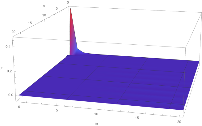
Figure 13: By setting $\kappa=i$ , $\mu=5i$ , we can see that the leading order term in $\mathcal{I}_{2}$ is given by the $m=0,n=0$ term. This further simplifies our calculation for the power spectrum.

$$\mathcal{I}_{2} \approx\frac{\Gamma(2\mu)\Gamma(-2\mu)}{\Gamma(\frac{1}{2}+\mu+\kappa)\Gamma(\frac{1}{2}-\mu-\kappa)}\frac{(-1)^{\frac{1}{2}+\mu}2}{(\frac{1}{2}+\mu)}$$ (129)

$$\,{}_{2}F_{1}\left(0,-\mu+\kappa+\frac{1}{2};1-2\mu;2\right)\,_{2}F_{1}\left(0,\mu-\kappa+\frac{1}{2};2\mu+1;2\right)\,_{2}F_{1}\left(1,\frac{1}{2}+\mu;\frac{3}{2}+\mu;-1\right)$$

$$=\frac{ie^{-i\pi\mu}}{2\mu}\csc(2\pi\mu)\cos(\pi(\kappa+\mu))\left(\psi^{(0)}\left(\frac{\mu}{2}+\frac{1}{4}\right)-\psi^{(0)}\left(\frac{\mu}{2}+\frac{3}{4}\right)\right)~{}.$$

We can easily generalized the analytic expression of the power spectrum to the case large mass limit. Similar results can be obtained in Tolley:2009fg ; Achucarro:2010jv ; Achucarro:2012sm ; Gwyn:2012mw ; Chen:2012ge ; Pi:2012gf ; An:2017hlx ; Tong:2017iat ; Iyer:2017qzw .

Appendix E Bispectrum in the Large Mass Limit

In this section, we derive the analytical expression for the bispectrum in the large mass limit. The large mass limit of the bispectrum in the quasi-single field model with neutral scalar particles is obtained in Gong:2013sma . After integrating out the massive field, an equilateral non-Gaussianity is obtained. This part contains no clock signal, however, it is the dominant contribution in the large mass limit since it is only suppressed by $1/|\mu|^{2}$ whereas the clock signal is supressed by $\exp(-\pi|\mu|)$ in the large mass limit. In this section, we like to derive the bispectrum by integrating out the massive charged scalar particles.

First, we calculate the second term of the bispectrum, we can write it as

$$\langle\zeta_{\mathbf{k}_{1}}\zeta_{\mathbf{k}_{2}}\zeta_{\mathbf{k}_{3}}\rangle^{\prime(2)} =2c_{2}c^{*}_{3}\frac{H^{3}e^{i\pi\kappa}}{128\epsilon^{3}k_{1}k_{2}k^{4}_{3}M_{\rm pl}^{6}}{\rm Re}\bigg{[}\int_{0}^{\infty}dx_{1}\frac{e^{-ix_{1}}W_{\kappa,\mu}(-2ix_{1})}{x_{1}}\int_{x_{1}}^{\infty}dx_{2}x_{2}e^{-i\frac{k_{1}+k_{2}}{k_{3}}x_{2}}W_{-\kappa,-\mu}(2ix_{2})\bigg{]}$$

$$+(\kappa\rightarrow-\kappa,c_{2}\rightarrow c_{2}^{*},c_{3}^{*}\rightarrow c_{3})~{}.$$ (130)

We expand the Whittaker function in the limit $x\rightarrow 0$, the first layer of integral is evaluated to

$$\int_{x_{1}}^{\infty}dx_{2}x_{2}e^{-i\frac{k_{1}+k_{2}}{k_{3}}x_{2}}\frac{(2ix_{2})^{1/2-\mu}\Gamma(2\mu)}{\Gamma\left(\kappa+\mu+\frac{1}{2}\right)}\sim-(2i)^{\frac{1}{2}-\mu}\frac{\Gamma(2\mu)}{\Gamma(\kappa+\mu+\frac{1}{2})}\frac{(x_{1})^{\frac{5}{2}-\mu}}{-\mu+\frac{5}{2}}e^{-i\frac{k_{1}+k_{2}}{k_{3}}x_{1}}~{}.$$ (131)

Inserting it into the second integral

$$\int_{0}^{\infty}dx_{1}\frac{e^{-ix_{1}}}{x_{1}}\frac{(-2ix_{1})^{1/2+\mu}\Gamma(-2\mu)}{\Gamma\left(-\kappa-\mu+\frac{1}{2}\right)}(-1)(2i)^{\frac{1}{2}-\mu}\frac{\Gamma(2\mu)}{\Gamma(\kappa+\mu+\frac{1}{2})}\frac{(x_{1})^{\frac{5}{2}-\mu}}{-\mu+\frac{5}{2}}e^{-i\frac{k_{1}+k_{2}}{k_{3}}x_{1}}$$

$$=(2i)(-1)^{\frac{3}{2}+\mu}\frac{\Gamma(2\mu)\Gamma(-2\mu)}{\Gamma(\kappa+\mu+\frac{1}{2})\Gamma(-\kappa-\mu+\frac{1}{2})(-\mu+\frac{5}{2})}\int_{0}^{\infty}dx_{1}x_{1}^{2}e^{-ix_{1}\frac{k_{1}+k_{2}+k_{3}}{k_{3}}}$$

$$=2(-1)^{\frac{1}{2}+\mu}\frac{\csc(2\pi\mu)\cos(\pi(\kappa+\mu))}{\mu(\mu-\frac{5}{2})}\bigg{(}\frac{k_{3}}{k_{1}+k_{2}+k_{3}}\bigg{)}^{3}~{}.$$ (132)

Hence, the second term of the bispectrum in the large mass limit can be expressed as

$$\langle\zeta_{\mathbf{k}_{1}}\zeta_{\mathbf{k}_{2}}\zeta_{\mathbf{k}_{3}}\rangle^{\prime(2)} =2c_{2}c^{*}_{3}\frac{H^{3}e^{i\pi\kappa}}{128\epsilon^{3}M_{\rm pl}^{6}k_{1}k_{2}k_{3}(k_{1}+k_{2}+k_{3})^{3}}{\rm Re}\left[2(-1)^{\frac{1}{2}+\mu}\frac{\csc(2\pi\mu)\cos(\pi(\kappa+\mu))}{\mu(\mu-\frac{5}{2})}\right]$$

$$+(\kappa\rightarrow-\kappa,c_{2}\rightarrow c_{2}^{*},c_{3}^{*}\rightarrow c_{3})~{}.$$ (133)

We can get the third term of the bispectrum in the large mass limit in the similar way.

$$\langle\zeta_{\mathbf{k}_{1}}\zeta_{\mathbf{k}_{2}}\zeta_{\mathbf{k}_{3}}\rangle^{\prime(3)} =2c_{2}c^{*}_{3}\frac{H^{3}e^{i\pi\kappa}}{128\epsilon^{3}M_{\rm pl}^{6}k_{1}k_{2}k_{3}(k_{1}+k_{2}+k_{3})^{3}}{\rm Re}\left[2(-1)^{\frac{1}{2}-\mu}\frac{\csc(2\pi\mu)\cos(\pi(\kappa+\mu))}{\mu(\mu-\frac{1}{2})}\right]$$

$$+(\kappa\rightarrow-\kappa,c_{2}\rightarrow c_{2}^{*},c_{3}^{*}\rightarrow c_{3})~{}.$$ (134)

Appendix F Analytical Expression for the Clock Signal

In this section, we compute the analytical expression for the clock signal following the standard approach developed in Arkani-Hamed:2015bza . In order to calculate the clock signal of primordial bispectrum analytically, we first simplify the propagators $D_{++}$, $D_{+-}$, $D_{-+}$, and $D_{--}$ in the following way. Using the late time behavior (12) and focusing on the non-local terms

$$v_{\mathbf{k}}(\tau_{1})v^{*}_{\mathbf{k}}(\tau_{2})=\frac{e^{-\pi|\mu|}}{a(\tau_{1})a(\tau_{2})4k|\mu|}\bigg{(} |\alpha|^{2}M_{\kappa,\mu}(2ki\tau_{1})(M_{\kappa,\mu}(2ik\tau_{2}))^{*}+\alpha\beta^{*}M_{\kappa,\mu}(2ki\tau_{1})M_{\kappa,\mu}(2ik\tau_{2})$$

$$+\alpha^{*}\beta(M_{\kappa,\mu}(2ki\tau_{1}))^{*}(M_{\kappa,\mu}(2ik\tau_{2}))^{*}+|\beta|^{2}(M_{\kappa,\mu}(2ki\tau_{1}))^{*}M_{\kappa,\mu}(2ik\tau_{2})\bigg{)}~{},$$ (135)

$$v^{*}_{\mathbf{k}}(\tau_{1})v_{\mathbf{k}}(\tau_{2})=\frac{e^{-\pi|\mu|}}{a(\tau_{1})a(\tau_{2})4k|\mu|}\bigg{(} |\alpha|^{2}(M_{\kappa,\mu}(2ki\tau_{1}))^{*}M_{\kappa,\mu}(2ik\tau_{2})+\alpha\beta^{*}M_{\kappa,\mu}(2ki\tau_{1})M_{\kappa,\mu}(2ik\tau_{2})$$

$$+\alpha^{*}\beta(M_{\kappa,\mu}(2ki\tau_{1}))^{*}(M_{\kappa,\mu}(2ik\tau_{2}))^{*}+|\beta|^{2}M_{\kappa,\mu}(2ki\tau_{1})(M_{\kappa,\mu}(2ik\tau_{2}))^{*}\bigg{)}~{},$$ (136)

from where we know that only $|\alpha|^{2}$ and $|\beta|^{2}$ terms are different. However, the $|\alpha|^{2}$ and $|\beta|^{2}$ terms are local, and hence, do not contribute to the clock signal.In order to understand the bispectrum in the squeeze limt ( $\alpha\beta^{*}$ and $\alpha^{*}\beta$ ), the four types of propagators $D_{++}$, $D_{+-}$, $D_{-+}$ and $D_{--}$, defined in (II) becomes identical.

$$D({\mathbf{k}},\tau_{1},\tau_{2})\equiv D_{++}({\mathbf{k}},\tau_{1},\tau_{2})=D_{-+}({\mathbf{k}},\tau_{1},\tau_{2})=D_{+-}({\mathbf{k}},\tau_{1},\tau_{2})=D_{--}({\mathbf{k}},\tau_{1},\tau_{2})$$

$$=\frac{e^{-\pi|\mu|}}{a(\tau_{1})a(\tau_{2})4k|\mu|}\bigg{(}\alpha\beta^{*}M_{\kappa,\mu}(2ki\tau_{1})M_{\kappa,\mu}(2ik\tau_{2})+\alpha^{*}\beta(M_{\kappa,\mu}(2ki\tau_{1}))^{*}(M_{\kappa,\mu}(2ik\tau_{2}))^{*}\bigg{)}~{}.$$ (137)

The squeezed limit bispectrum can be calculated for all orders in the $(k_{1}/k_{3})$ expansion. However, for simplicity, we focus on the first order $(k_{1}/k_{3})$ expansion, where the Whittacker M is expanded as

$$M_{\kappa,\mu}(z)=z^{\mu+1/2}+\mathcal{O}(z^{\mu+3/2})~{}.$$ (138)

Taking the effective mass to be $e_{0}^{2}E^{2}/H^{4}+m^{2}/H^{2}>9/4$. The charged massive scalar propagator becomes

$$D({\mathbf{k}},\tau_{1},\tau_{2}) \equiv D_{++}({\mathbf{k}},\tau_{1},\tau_{2})=D_{-+}({\mathbf{k}},\tau_{1},\tau_{2})=D_{+-}({\mathbf{k}},\tau_{1},\tau_{2})=D_{--}({\mathbf{k}},\tau_{1},\tau_{2})$$

$$=\frac{e^{-\pi|\mu|}}{a(\tau_{1})a(\tau_{2})4k|\mu|}\bigg{(}\alpha^{*}\beta(-4k^{2}\tau_{1}\tau_{2})^{-\mu+1/2}+{\rm c.c}\bigg{)}~{}.$$ (139)

The bispectrum is further simplified to

$$\langle\zeta_{\mathbf{k}_{1}}\zeta_{\mathbf{k}_{2}}\zeta_{\mathbf{k}_{3}}\rangle^{\prime}=2c_{2}c_{3}^{*}{\rm Re}\Bigg{[}\int_{-\infty}^{0}\int_{-\infty}^{0} \frac{d\tau_{1}}{(-H\tau_{1})^{3}}\frac{d\tau_{2}}{(-H\tau_{2})^{2}}[\partial_{\tau_{1}}G_{++}({\mathbf{k}_{3}},\tau_{1},0)-\partial_{\tau_{1}}G_{-+}({\mathbf{k}_{3}},\tau_{1},0)]D({\mathbf{k}_{3}},\tau_{1},\tau_{2})$$

$$\partial_{\tau_{2}}G_{++}({\mathbf{k}_{1}},\tau_{2},0)\partial_{\tau_{2}}G_{++}({\mathbf{k}_{2}},\tau_{2},0)\Bigg{]}+(\kappa\rightarrow-\kappa,c_{2}\rightarrow c_{2}^{*},c_{3}^{*}\rightarrow c_{3})~{}.$$ (140)

After evaluation, the bispectrum becomes

$$\langle\zeta_{\mathbf{k}_{1}}\zeta_{\mathbf{k}_{2}}\zeta_{\mathbf{k}_{3}}\rangle^{\prime}=c_{2}c^{*}_{3}{\rm Re}\Bigg{[}f(\mu,\kappa)\frac{2^{2\mu}H^{3}}{16k_{1}k_{2}k_{3}^{3/2}k_{12}^{5/2}M_{\rm pl}^{6}\epsilon^{3}}\bigg{(}\frac{k_{1}+k_{2}}{k_{3}}\bigg{)}^{-\mu}\Bigg{]}+(\kappa\rightarrow-\kappa,c_{2}\rightarrow c_{2}^{*},c_{3}^{*}\rightarrow c_{3})~{},$$ (141)

where the prefactor is given by

$$f(\mu,\kappa)\equiv e^{i\pi\kappa}\frac{\Gamma(-2\mu)^{2}\Gamma\left(\frac{1}{2}+\mu\right)\Gamma\left(\frac{5}{2}+\mu\right)}{\Gamma(\frac{1}{2}-\mu-\kappa)\Gamma(\frac{1}{2}+\mu-\kappa)}\left(1+\text{sin}\left(\pi\mu\right)\right)~{}.$$ (142)

The shape function is

$$S(k_{1},k_{2},k_{3})=\frac{c_{2}c_{3}^{*}}{HM_{\rm pl}^{2}\epsilon}{\rm Re}\bigg{[}f(\mu,\kappa)\frac{2^{2\mu-2}k_{1}k_{2}k_{3}^{1/2}}{k_{12}^{5/2}}\bigg{(}\frac{k_{1}+k_{2}}{k_{3}}\bigg{)}^{-\mu}\bigg{]}+(\kappa\rightarrow-\kappa,c_{2}\rightarrow c_{2}^{*},c_{3}^{*}\rightarrow c_{3})~{}.$$ (143)

References

(1)
J. S. Schwinger,
“On gauge invariance and vacuum polarization,”
Phys. Rev. 82, 664 (1951).
(2)
A. Di Piazza, C. Muller, K. Z. Hatsagortsyan and C. H. Keitel,
“Extremely high-intensity laser interactions with fundamental quantum systems,”
Rev. Mod. Phys. 84, 1177 (2012)
[arXiv:1111.3886 [hep-ph]].
(3)
R. Ruffini, G. Vereshchagin and S. S. Xue,
“Electron-positron pairs in physics and astrophysics: from heavy nuclei to black holes,”
Phys. Rept. 487, 1 (2010)
[arXiv:0910.0974 [astro-ph.HE]].
(4)
W. Tangarife, K. Tobioka, L. Ubaldi and T. Volansky,
“Dynamics of Relaxed Inflation,”
JHEP 1802, 084 (2018)
[arXiv:1706.03072 [hep-ph]].
(5)
W. Tangarife, K. Tobioka, L. Ubaldi and T. Volansky,
“Relaxed Inflation,”
arXiv:1706.00438 [hep-ph].
(6)
T. E. Clarke, P. P. Kronberg and H. Boehringer,
“A New radio - X-ray probe of galaxy cluster magnetic fields,”
Astrophys. J. 547, L111 (2001)
[astro-ph/0011281].
(7)
F. Govoni and L. Feretti,
“Magnetic field in clusters of galaxies,”
Int. J. Mod. Phys. D 13, 1549 (2004)
[astro-ph/0410182].
(8)
C. Vogt and T. A. Ensslin,
“A Bayesian view on Faraday rotation maps - Seeing the magnetic power spectra in galaxy clusters,”
Astron. Astrophys. 434, 67 (2005)
[astro-ph/0501211].
(9)
K. Dolag, M. Kachelriess, S. Ostapchenko and R. Tomas,
“Lower limit on the strength and filling factor of extragalactic magnetic fields,”
Astrophys. J. 727, L4 (2011)
[arXiv:1009.1782 [astro-ph.HE]].
(10)
A. Neronov and I. Vovk,
“Evidence for strong extragalactic magnetic fields from Fermi observations of TeV blazars,”
Science 328, 73 (2010)
[arXiv:1006.3504 [astro-ph.HE]].
(11)
F. Tavecchio, G. Ghisellini, L. Foschini, G. Bonnoli, G. Ghirlanda and P. Coppi,
“The intergalactic magnetic field constrained by Fermi/LAT observations of the TeV blazar 1ES 0229+200,”
Mon. Not. Roy. Astron. Soc. 406, L70 (2010)
[arXiv:1004.1329 [astro-ph.CO]].
(12)
M. S. Turner and L. M. Widrow,
“Inflation Produced, Large Scale Magnetic Fields,”
Phys. Rev. D 37, 2743 (1988).
(13)
B. Ratra,
“Cosmological ’seed’ magnetic field from inflation,”
Astrophys. J. 391, L1 (1992).
(14)
A. Dolgov,
“Breaking of conformal invariance and electromagnetic field generation in the universe,”
Phys. Rev. D 48, 2499 (1993)
[hep-ph/9301280].
(15)
M. Gasperini, M. Giovannini and G. Veneziano,
“Primordial magnetic fields from string cosmology,”
Phys. Rev. Lett. 75, 3796 (1995)
[hep-th/9504083].
(16)
M. Giovannini,
“Magnetogenesis and the dynamics of internal dimensions,”
Phys. Rev. D 62, 123505 (2000)
[hep-ph/0007163].
(17)
K. Bamba and J. Yokoyama,
“Large scale magnetic fields from inflation in dilaton electromagnetism,”
Phys. Rev. D 69, 043507 (2004)
[astro-ph/0310824].
(18)
K. Bamba and M. Sasaki,
“Large-scale magnetic fields in the inflationary universe,”
JCAP 0702, 030 (2007)
[astro-ph/0611701].
(19)
M. Giovannini and K. E. Kunze,
“Magnetized CMB observables: A Dedicated numerical approach,”
Phys. Rev. D 77, 063003 (2008)
[arXiv:0712.3483 [astro-ph]].
(20)
J. Martin and J. Yokoyama,
“Generation of Large-Scale Magnetic Fields in Single-Field Inflation,”
JCAP 0801, 025 (2008)
[arXiv:0711.4307 [astro-ph]].
(21)
K. Subramanian,
“Magnetic fields in the early universe,”
Astron. Nachr. 331, 110 (2010)
[arXiv:0911.4771 [astro-ph.CO]].
(22)
A. Kandus, K. E. Kunze and C. G. Tsagas,
“Primordial magnetogenesis,”
Phys. Rept. 505, 1 (2011)
[arXiv:1007.3891 [astro-ph.CO]].
(23)
R. Durrer,
“Cosmic Magnetic Fields and the CMB,”
New Astron. Rev. 51, 275 (2007)
[astro-ph/0609216].
(24)
K. Atmjeet, I. Pahwa, T. R. Seshadri and K. Subramanian,
“Cosmological Magnetogenesis From Extra-dimensional Gauss Bonnet Gravity,”
Phys. Rev. D 89, no. 6, 063002 (2014)
[arXiv:1312.5815 [astro-ph.CO]].
(25)
T. Fujita, R. Namba, Y. Tada, N. Takeda and H. Tashiro,
“Consistent generation of magnetic fields in axion inflation models,”
JCAP 1505, no. 05, 054 (2015)
[arXiv:1503.05802 [astro-ph.CO]].
(26)
G. Domènech, C. Lin and M. Sasaki,
“Inflationary Magnetogenesis with Broken Local U(1) Symmetry,”
EPL 115, no. 1, 19001 (2016)
[arXiv:1512.01108 [astro-ph.CO]].
(27)
C. Stahl,
“Schwinger effect impacting primordial magnetogenesis,”
arXiv:1806.06692 [hep-th].
(28)
V. Demozzi, V. Mukhanov and H. Rubinstein,
“Magnetic fields from inflation?,”
JCAP 0908, 025 (2009)
[arXiv:0907.1030 [astro-ph.CO]].
(29)
M. a. Watanabe, S. Kanno and J. Soda,
“Inflationary Universe with Anisotropic Hair,”
Phys. Rev. Lett. 102, 191302 (2009)
[arXiv:0902.2833 [hep-th]].
(30)
H. Kitamoto,
“Schwinger Effect in Inflaton-Driven Electric Field,”
arXiv:1807.03753 [hep-th].
(31)
S. Kanno, J. Soda and M. a. Watanabe,
“Cosmological Magnetic Fields from Inflation and Backreaction,”
JCAP 0912, 009 (2009)
[arXiv:0908.3509 [astro-ph.CO]].
(32)
S. P. Kim and D. N. Page,
“Schwinger Pair Production in dS(2) and AdS(2),”
Phys. Rev. D 78, 103517 (2008)
[arXiv:0803.2555 [hep-th]].
(33)
M. B. Fröb, J. Garriga, S. Kanno, M. Sasaki, J. Soda, T. Tanaka and A. Vilenkin,
“Schwinger effect in de Sitter space,”
JCAP 1404, 009 (2014)
[arXiv:1401.4137 [hep-th]].
(34)
C. Stahl, E. Strobel and S. S. Xue,
“Fermionic current and Schwinger effect in de Sitter spacetime,”
Phys. Rev. D 93, no. 2, 025004 (2016)
[arXiv:1507.01686 [gr-qc]].
(35)
T. Kobayashi and N. Afshordi,
“Schwinger Effect in 4D de Sitter Space and Constraints on Magnetogenesis in the Early Universe,”
JHEP 1410, 166 (2014)
[arXiv:1408.4141 [hep-th]].
(36)
M. Banyeres, G. Domènech and J. Garriga,
“Vacuum birefringence and the Schwinger effect in (3+1) de Sitter,”
arXiv:1809.08977 [hep-th].
(37)
T. Hayashinaka and J. Yokoyama,
“Point splitting renormalization of Schwinger induced current in de Sitter spacetime,”
JCAP 1607, no. 07, 012 (2016)
[arXiv:1603.06172 [hep-th]].
(38)
J. J. Geng, B. F. Li, J. Soda, A. Wang, Q. Wu and T. Zhu,
“Schwinger Pair Production by Electric Field Coupled to Inflaton,”
JCAP 1802, no. 02, 018 (2018)
[arXiv:1706.02833 [gr-qc]].
(39)
T. Hayashinaka and S. S. Xue,
“Physical renormalization condition for de Sitter QED,”
Phys. Rev. D 97, no. 10, 105010 (2018)
[arXiv:1802.03686 [gr-qc]].
(40)
X. Chen and Y. Wang,
“Large non-Gaussianities with Intermediate Shapes from Quasi-Single Field Inflation,”
Phys. Rev. D 81 (2010) 063511
[arXiv:0909.0496 [astro-ph.CO]].
(41)
X. Chen and Y. Wang,
“Quasi-Single Field Inflation and Non-Gaussianities,”
JCAP 1004 (2010) 027
[arXiv:0911.3380 [hep-th]].
(42)
D. Baumann and D. Green,
“Signatures of Supersymmetry from the Early Universe,”
Phys. Rev. D 85, 103520 (2012)
[arXiv:1109.0292 [hep-th]].
(43)
N. Arkani-Hamed and J. Maldacena,
“Cosmological Collider Physics,”
arXiv:1503.08043 [hep-th].
(44)
L. H. Ford,
“Inflation Driven By A Vector Field,”
Phys. Rev. D 40, 967 (1989).
(45)
S. Yokoyama and J. Soda,
“Primordial statistical anisotropy generated at the end of inflation,”
JCAP 0808, 005 (2008)
[arXiv:0805.4265 [astro-ph]].
(46)
R. Emami, H. Firouzjahi, S. M. Sadegh Movahed and M. Zarei,
“Anisotropic Inflation from Charged Scalar Fields,”
JCAP 1102, 005 (2011)
[arXiv:1010.5495 [astro-ph.CO]].
(47)
J. Soda,
“Statistical Anisotropy from Anisotropic Inflation,”
Class. Quant. Grav. 29, 083001 (2012)
[arXiv:1201.6434 [hep-th]].
(48)
P. Adshead and A. Liu,
“Anisotropic Massive Gauge-flation,”
JCAP 1807, no. 07, 052 (2018)
[arXiv:1803.07168 [astro-ph.CO]].
(49)
H. W. H. Tahara, S. Nishi, T. Kobayashi and J. Yokoyama,
“Self-anisotropizing inflationary universe in Horndeski theory and beyond,”
JCAP 1807, no. 07, 058 (2018)
[arXiv:1805.00186 [gr-qc]].
(50)
J. D. Barrow and S. Hervik,
“Anisotropically inflating universes,”
Phys. Rev. D 73, 023007 (2006)
[gr-qc/0511127].
(51)
J. D. Barrow and S. Hervik,
“On the evolution of universes in quadratic theories of gravity,”
Phys. Rev. D 74, 124017 (2006)
[gr-qc/0610013].
(52)
J. D. Barrow and S. Hervik,
“Simple Types of Anisotropic Inflation,”
Phys. Rev. D 81, 023513 (2010)
[arXiv:0911.3805 [gr-qc]].
(53)
A. Maleknejad, M. M. Sheikh-Jabbari and J. Soda,
“Gauge Fields and Inflation,”
Phys. Rept. 528, 161 (2013)
[arXiv:1212.2921 [hep-th]].
(54)
R. Emami,
“Anisotropic Inflation and Cosmological Observations,”
arXiv:1511.01683 [astro-ph.CO].
(55)
P. Adshead and E. I. Sfakianakis,
“Fermion production during and after axion inflation,”
JCAP 1511, 021 (2015)
[arXiv:1508.00891 [hep-ph]].
(56)
P. Adshead, L. Pearce, M. Peloso, M. A. Roberts and L. Sorbo,
“Phenomenology of fermion production during axion inflation,”
JCAP 1806, no. 06, 020 (2018)
[arXiv:1803.04501 [astro-ph.CO]].
(57)
X. Chen, Y. Wang and Z. Z. Xianyu,
“Neutrino Signatures in Primordial Non-Gaussianities,”
JHEP 1809, 022 (2018)
[arXiv:1805.02656 [hep-ph]].
(59)
Y. Wang,
“Inflation, Cosmic Perturbations and Non-Gaussianities,”
Commun. Theor. Phys. 62, 109 (2014)
[arXiv:1303.1523 [hep-th]].
(60)
S. Kumar and R. Sundrum,
“Heavy-Lifting of Gauge Theories By Cosmic Inflation,”
JHEP 1805, 011 (2018)
[arXiv:1711.03988 [hep-ph]].
(61)
X. Chen, Y. Wang and Z. Z. Xianyu,
“Schwinger-Keldysh Diagrammatics for Primordial Perturbations,”
JCAP 1712, no. 12, 006 (2017)
[arXiv:1703.10166 [hep-th]].
(62)
Weinberg, Steven. Gravitation and cosmology: principles and applications of the general theory of relativity. Vol. 1. New York: Wiley, 1972.
(63)
S. M. Carroll,
San Francisco, USA: Addison-Wesley (2004) 513 p
(64)
R. Flauger, M. Mirbabayi, L. Senatore and E. Silverstein,
“Productive Interactions: heavy particles and non-Gaussianity,”
JCAP 1710, no. 10, 058 (2017)
[arXiv:1606.00513 [hep-th]].
(65)
X. Tong, Y. Wang and S. Zhou,
“Unsuppressed primordial standard clocks in warm quasi-single field inflation,”
JCAP 1806, no. 06, 013 (2018)
[arXiv:1801.05688 [hep-th]].
(66)
X. Chen, W. Z. Chua, Y. Guo, Y. Wang, Z. Z. Xianyu and T. Xie,
“Quantum Standard Clocks in the Primordial Trispectrum,”
JCAP 1805, no. 05, 049 (2018)
[arXiv:1803.04412 [hep-th]].
(67)
T. Noumi, M. Yamaguchi and D. Yokoyama,
“Effective field theory approach to quasi-single field inflation and effects of heavy fields,”
JHEP 1306, 051 (2013)
[arXiv:1211.1624 [hep-th]].
(68)
H. Lee, D. Baumann and G. L. Pimentel,
“Non-Gaussianity as a Particle Detector,”
JHEP 1612, 040 (2016)
[arXiv:1607.03735 [hep-th]].
(69)
X. Chen, Y. Wang and Z. Z. Xianyu,
“Loop Corrections to Standard Model Fields in Inflation,”
JHEP 1608, 051 (2016)
[arXiv:1604.07841 [hep-th]].
(70)
X. Chen, Y. Wang and Z. Z. Xianyu,
“Standard Model Background of the Cosmological Collider,”
Phys. Rev. Lett. 118, no. 26, 261302 (2017)
[arXiv:1610.06597 [hep-th]].
(71)
X. Chen, Y. Wang and Z. Z. Xianyu,
“Standard Model Mass Spectrum in Inflationary Universe,”
JHEP 1704, 058 (2017)
[arXiv:1612.08122 [hep-th]].
(72)
Y. P. Wu and J. Yokoyama,
“Loop corrections to primordial fluctuations from inflationary phase transitions,”
JCAP 1805, no. 05, 009 (2018)
[arXiv:1704.05026 [hep-th]].
(73)
S. Weinberg,
“Quantum contributions to cosmological correlations,”
Phys. Rev. D 72, 043514 (2005)
[hep-th/0506236].
(74)
L. Senatore and M. Zaldarriaga,
“On Loops in Inflation,”
JHEP 1012, 008 (2010)
[arXiv:0912.2734 [hep-th]].
(75)
L. Senatore and M. Zaldarriaga,
“On Loops in Inflation II: IR Effects in Single Clock Inflation,”
JHEP 1301, 109 (2013)
[arXiv:1203.6354 [hep-th]].
(76)
G. L. Pimentel, L. Senatore and M. Zaldarriaga,
“On Loops in Inflation III: Time Independence of zeta in Single Clock Inflation,”
JHEP 1207, 166 (2012)
[arXiv:1203.6651 [hep-th]].
(77)
E. Dimastrogiovanni, M. Fasiello and G. Tasinato,
“Probing the inflationary particle content: extra spin-2 field,”
JCAP 1808, no. 08, 016 (2018)
[arXiv:1806.00850 [astro-ph.CO]].
(78)
E. Bavarsad, S. P. Kim, C. Stahl and S. S. Xue,
“Effect of a magnetic field on Schwinger mechanism in de Sitter spacetime,”
Phys. Rev. D 97, no. 2, 025017 (2018)
[arXiv:1707.03975 [hep-th]].
(79)
T. Hayashinaka, T. Fujita and J. Yokoyama,
“Fermionic Schwinger effect and induced current in de Sitter space,”
JCAP 1607, no. 07, 010 (2016)
[arXiv:1603.04165 [hep-th]].
(80)
K. D. Lozanov, A. Maleknejad and E. Komatsu,
“Schwinger Effect by an Gauge Field during Inflation,”
arXiv:1805.09318 [hep-th].
(81)
A. Maleknejad and E. Komatsu,
“Production and Backreaction of Spin-2 Particles of Gauge Field during Inflation,”
arXiv:1808.09076 [hep-ph].
(82)
E. Dimastrogiovanni, M. Fasiello and T. Fujita,
“Primordial Gravitational Waves from Axion-Gauge Fields Dynamics,”
JCAP 1701, no. 01, 019 (2017)
[arXiv:1608.04216 [astro-ph.CO]].
(83)
C. Stahl and S. S. Xue,
“Schwinger effect and backreaction in de Sitter spacetime,”
Phys. Lett. B 760, 288 (2016)
[arXiv:1603.07166 [hep-th]].
(84)
E. Bavarsad, C. Stahl and S. S. Xue,
“Scalar current of created pairs by Schwinger mechanism in de Sitter spacetime,”
Phys. Rev. D 94, no. 10, 104011 (2016)
[arXiv:1602.06556 [hep-th]].
(85)
O. O. Sobol, E. V. Gorbar, M. Kamarpour and S. I. Vilchinskii,
“Influence of backreaction of electric fields and Schwinger effect on inflationary magnetogenesis,”
Phys. Rev. D 98, 063534 (2018)
[arXiv:1807.09851 [hep-ph]].
(86)
H. Firouzjahi, M. A. Gorji, S. A. Hosseini Mansoori, A. Karami and T. Rostami,
arXiv:1812.07464 [hep-th].
(87)
K. Dimopoulos, M. Karciauskas, D. H. Lyth and Y. Rodriguez,
JCAP 0905, 013 (2009)
doi:10.1088/1475-7516/2009/05/013
[arXiv:0809.1055 [astro-ph]].
(88)
K. Dimopoulos, M. Karciauskas and J. M. Wagstaff,
Phys. Lett. B 683, 298 (2010)
doi:10.1016/j.physletb.2009.12.024
[arXiv:0909.0475 [hep-ph]].
(89)
J. C. Bueno Sanchez and K. Dimopoulos,
JCAP 1401, 012 (2014)
doi:10.1088/1475-7516/2014/01/012
[arXiv:1308.3739 [hep-ph]].
(90)
A. J. Tolley and M. Wyman,
“The Gelaton Scenario: Equilateral non-Gaussianity from multi-field dynamics,”
Phys. Rev. D 81, 043502 (2010)
[arXiv:0910.1853 [hep-th]].
(91)
A. Achucarro, J. O. Gong, S. Hardeman, G. A. Palma and S. P. Patil,
“Mass hierarchies and non-decoupling in multi-scalar field dynamics,”
Phys. Rev. D 84, 043502 (2011)
[arXiv:1005.3848 [hep-th]].
(92)
A. Achucarro, J. O. Gong, S. Hardeman, G. A. Palma and S. P. Patil,
“Effective theories of single field inflation when heavy fields matter,”
JHEP 1205, 066 (2012)
[arXiv:1201.6342 [hep-th]].
(93)
X. Chen and Y. Wang,
“Quasi-Single Field Inflation with Large Mass,”
JCAP 1209, 021 (2012)
[arXiv:1205.0160 [hep-th]].
(94)
S. Pi and M. Sasaki,
“Curvature Perturbation Spectrum in Two-field Inflation with a Turning Trajectory,”
JCAP 1210, 051 (2012)
[arXiv:1205.0161 [hep-th]].
(95)
R. Gwyn, G. A. Palma, M. Sakellariadou and S. Sypsas,
“Effective field theory of weakly coupled inflationary models,”
JCAP 1304, 004 (2013)
[arXiv:1210.3020 [hep-th]].
(96)
H. An, M. McAneny, A. K. Ridgway and M. B. Wise,
“Quasi Single Field Inflation in the non-perturbative regime,”
JHEP 1806, 105 (2018)
[arXiv:1706.09971 [hep-ph]].
(97)
X. Tong, Y. Wang and S. Zhou,
“On the Effective Field Theory for Quasi-Single Field Inflation,”
JCAP 1711, no. 11, 045 (2017)
[arXiv:1708.01709 [astro-ph.CO]].
(98)
A. V. Iyer, S. Pi, Y. Wang, Z. Wang and S. Zhou,
“Strongly Coupled Quasi-Single Field Inflation,”
JCAP 1801, no. 01, 041 (2018)
[arXiv:1710.03054 [hep-th]].
(99)
J. O. Gong, S. Pi and M. Sasaki,
“Equilateral non-Gaussianity from heavy fields,”
JCAP 1311, 043 (2013)
[arXiv:1306.3691 [hep-th]].