Simple preparation of Bell and GHZ states using ultrastrong-coupling circuit QED

Abstract

The ability to entangle quantum systems is crucial for many applications in quantum technology, including quantum communication and quantum computing. Here, we propose a new, simple, and versatile setup for deterministically creating Bell and Greenberger-Horne-Zeilinger (GHZ) states between photons of different frequencies in a two-step protocol. The setup consists of a quantum bit (qubit) coupled ultrastrongly to three photonic resonator modes. The only operations needed in our protocol are to put the qubit in a superposition state, and then tune its frequency in and out of resonance with sums of the resonator-mode frequencies. By choosing which frequency we tune the qubit to, we select which entangled state we create. We show that our protocol can be implemented with high fidelity using feasible experimental parameters in state-of-the-art circuit quantum electrodynamics. One possible application of our setup is as a node distributing entanglement in a quantum network.

I Introduction

Quantum entanglement Horodecki et al. (2009) plays a key role in quantum communication Gisin and Thew (2007), quantum computing Nielsen and Chuang (2000); Ladd et al. (2010); Buluta et al. (2011), and other quantum information processing Wendin (2017); Gu et al. (2017); Flamini et al. (2018). To give just a few examples, quantum teleportation Bennett et al. (1993), quantum key distribution Ekert (1991), quantum secret sharing Hillery et al. (1999), quantum secure direct communication Long and Liu (2002); Deng et al. (2003), and quantum repeaters Briegel et al. (1998); Li and Deng (2015), are some of the quantum communication protocols that require entangling quantum systems.

The simplest examples of entangled states are known as Bell states. They are four maximally entangled states involving two quantum bits (qubits, two-level systems with ground state $|0\rangle$ and excited state $|1\rangle$):

$$|\Phi_{\pm}\rangle = \frac{1}{\sqrt{2}}\left(|00\rangle\pm|11\rangle\right),$$ (1)

$$|\Psi_{\pm}\rangle = \frac{1}{\sqrt{2}}\left(|01\rangle\pm|10\rangle\right).$$ (2)

The Bell states are of fundamental importance in both quantum cryptography and quantum teleportation. With $N\geq 3$ qubits, maximally entangled states such as the Greenberger-Horne-Zeilinger (GHZ) states Greenberger et al. (1989); Bouwmeester et al. (1999),

$$|\Psi_{\rm GHZ}\rangle=\frac{1}{\sqrt{2}}\left(|0\rangle^{\otimes N}+|1\rangle^{\otimes N}\right),$$ (3)

and the W states Dür et al. (2000),

$$|\Psi_{\rm W}\rangle=\frac{1}{\sqrt{N}}\left(|100\ldots 0\rangle+|010\ldots 0\rangle+\ldots+|000\ldots 1\rangle\right),$$ (4)

are not only of intrinsic interest but also of great practical importance. New systems and methods for preparing and measuring such entangled states has therefore been sought intensively for a long time Aspect et al. (1982); Weihs et al. (1998); Mølmer and Sørensen (1999); Pan et al. (2000); Zhao et al. (2003); Wei et al. (2006); Steffen et al. (2006); Coelho et al. (2009); Bishop et al. (2009); Zhang et al. (2009); DiCarlo et al. (2010); Wang et al. (2010); Hasegawa et al. (2010); Pan et al. (2012); Ristè et al. (2013); Su et al. (2014); Johansson et al. (2014); Zang et al. (2015); Yang et al. (2016); Kang et al. (2016); Tashima et al. (2016); Zhang et al. (2016); Ritboon et al. (2017); Erhard et al. (2017); Qin et al. (2018); Cruz et al. (2018), and remains a very active field of research. In recent years, entanglement of ten or more qubits has been demonstrated in various experimental setups Monz et al. (2011); Wang et al. (2016); Hou et al. (2016); Song et al. (2017); Wang et al. (2018).

In this article, we propose a simple method for the deterministic preparation of Bell and GHZ states using ultrastrong coupling (USC) Kockum et al. (2018); Forn-Díaz et al. (2018) between light and matter. In this regime of light-matter interaction, the coupling strength $g$ becomes comparable to the bare transition frequencies $\omega$ in the system. In the past decade, USC has been realized in several experimental systems Kockum et al. (2018), including intersubband polaritons Anappara et al. (2009); Günter et al. (2009); Geiser et al. (2012); Askenazi et al. (2017) and Landau polaritons Muravev et al. (2011); Scalari et al. (2012); Bayer et al. (2017) in quantum wells, superconducting circuits Niemczyk et al. (2010); Forn-Díaz et al. (2010); Chen et al. (2017); Yoshihara et al. (2017); Forn-Díaz et al. (2017), organic cavities in photonic cavities Schwartz et al. (2011); Gambino et al. (2014); Barachati et al. (2018); Genco et al. (2018), and optomechanical systems George et al. (2016); Benz et al. (2016). Out of these systems, we believe our proposal is most suited for superconducting circuits, i.e., the circuit version of cavity quantum electrodynamics (QED) Haroche (2013) known as circuit QED You and Nori (2011); Gu et al. (2017). The reason for this is that the circuit-QED experiments are the only ones that have demonstrated USC with single (although artificial) atoms.

Although USC leads to much interesting physics De Liberato et al. (2007, 2009); Ashhab and Nori (2010); Casanova et al. (2010); Ai et al. (2010); Cao et al. (2010, 2011); Stassi et al. (2013); Ridolfo et al. (2013); Garziano et al. (2013, 2014); Huang and Law (2014); Sanchez-Burillo et al. (2014); De Liberato (2014); Zhao et al. (2015); Lolli et al. (2015); Cirio et al. (2016); Di Stefano et al. (2017); Macrì et al. (2018), in this article, we are only using the fact that it enables higher-order processes that do not conserve the number of excitations in the system Zhu et al. (2013); Ma and Law (2015); Garziano et al. (2015, 2016); Kockum et al. (2017a); Stassi et al. (2017); Kockum et al. (2017b). These processes include multiphoton Rabi oscillations Garziano et al. (2015), a single photon exciting two spatially separated qubits Garziano et al. (2016), and analogues of almost all nonlinear-optics phenomena Kockum et al. (2017a), including various frequency-conversion schemes Kockum et al. (2017b).

Our proposal for generating Bell and GHZ states builds on ideas from Refs. Kockum et al. (2017b); Stassi et al. (2017). In Ref. Kockum et al. (2017b), we showed how to realize frequency conversion of photons in two resonators (or resonator modes) ultrastrongly coupled to a single qubits, and that these processes can be well controlled by tuning the qubit frequency in and out of resonance conditions for these processes. The ability to tune the qubit frequency in this way is available in many circuit-QED experiments. In the present work, we consider setups with the qubit coupled ultrastrongly to two or three resonator modes. The key difference to Ref. Kockum et al. (2017b), which allows us to create various entangled states between photons in the different resonator modes, is that we first prepare the qubit in a superposition, and then use frequency-conversion processes to transfer this superposition to the photons.

For example, to prepare a Bell state with photons in the first two resonator modes, we first prepare the qubit in a superposition state with equal amplitudes for being in the ground state and for being in the excited state. We then tune the qubit frequency to equal the sum of the transition frequencies for the two resonator modes. This resonance condition enables a higher-order process that transfers the qubit excitation to photons in the resonator modes and back in a Rabi oscillation. By detuning the qubit just when the excitation is fully in the resonator modes, we end up with a Bell state of the type shown in Eq. (1).

Our proposed setup is a simple and versatile entanglement generator. The only operations required are to prepare one qubit in a superposition state and then tuning it in and out of resonance. The same setup can both generate Bell states for any pair of resonator modes and GHZ states for all the modes. The only part of the protocol that needs to be adjusted, to choose which entangled state to generate, is which value the qubit frequency is tuned to. This could be useful in quantum information processing, e.g., for distributing entanglement at a node in a quantum network Kimble (2008); Wehner et al. (2018). Our setup is also versatile in the sense that we can generate entanglement between photons of several different colors (the frequencies are given by the resonator-mode frequencies); it could be said that we create “rainbow” entangled states, similar to Ref. Coelho et al. (2009).

This article is organized as follows. In Sec. II, we describe our system in detail. We plot the energy levels of the system Hamiltonian to illustrate how tuning the qubit frequency enables the different entangling processes we want, and we give analytical expressions for the effective interaction strength for these processes, which sets the time needed to create the entangled state. We also describe how we model losses in the system. In Sec. III, we explain the details of our protocol for entanglement generation and present results of full numerical simulations of these protocols, using experimentally feasible parameters and including losses of varying degree. We then conclude and give an outlook for future work and applications in Sec. IV. The analytical calculations for the effective interaction strengths are presented in detail in Appendices A and B.

II Description of the model

II.1 Hamiltonian

We consider a quantum system consisting of three non-degenerate resonator modes (labelled $a$, $b$, $c$) coupled ultrastrongly to a two-level system (a qubit, labelled $q$), possibly with symmetry-broken potentials. The Hamiltonian describing this system is the generalized quantum Rabi Hamiltonian ($\hbar=1$ throughout this article)

$$\hat{H} = \omega_{a}\hat{a}^{\dagger}\hat{a}+\omega_{b}\hat{b}^{\dagger}\hat{b}+\omega_{c}\hat{c}^{\dagger}\hat{c}+\frac{\omega_{q}}{2}\hat{\sigma}_{z}$$ (5)

$$+\left[g_{a}\left(\hat{a}^{\dagger}+\hat{a}\right)+g_{b}\left(\hat{b}^{\dagger}+\hat{b}\right)+g_{c}\left(\hat{c}^{\dagger}+\hat{c}\right)\right]$$

$$\times\left(\hat{\sigma}_{x}\cos\theta+\hat{\sigma}_{z}\sin\theta\right),$$

where $\omega_{j}$ is the transition frequency of resonator mode $j$, $\omega_{q}$ is the qubit frequency, and $g_{j}$ is the strength of the coupling between resonator $j$ and the qubit. The operators $\hat{a}$, $\hat{b}$, and $\hat{c}$ ($\hat{a}^{\dagger}$, $\hat{b}^{\dagger}$, and $\hat{c}^{\dagger}$) are the annihilation (creation) operators of the resonator modes $a$, $b$, and $c$, respectively. The qubit degrees of freedom are described by the Pauli matrices $\hat{\sigma}_{z}$ and $\hat{\sigma}_{x}$. The angle $\theta$ parameterizes the amount of longitudinal and transversal coupling between the qubit and the resonators.

This mix of longitudinal and transversal coupling can be realized in circuit-QED experiments with flux qubits You et al. (2007); Deppe et al. (2008); Forn-Díaz et al. (2010); Niemczyk et al. (2010); Baust et al. (2016); Yoshihara et al. (2017). Note that the presence of the longitudinal coupling term in Eq. (5) is necessary to generate photonic Bell states in our scheme, since that requires converting one qubit excitation into two photons, which neither conserves the number of excitations in the system nor their parity. However, to generate photonic GHZ states, the transversal coupling, which conserves parity, is sufficient, since in this case one qubit excitation is converted into three photons. Thus, if one only wishes to generate GHZ states, the standard quantum Rabi Hamiltonian ($\theta=0$) for multiple resonator modes can be used.

II.2 Master equation and numerical methods

To include the effect of decoherence in our system, we use a master equation on the Lindblad form in our numerical simulations. Following Refs. Breuer and Petruccione (2002); Beaudoin et al. (2011); Ridolfo et al. (2012), we express the system-bath interaction Hamiltonian in the basis formed by the energy eigenstates of $\hat{H}$ from Eq. (5). By applying the standard Markov approximation and tracing out the reservoir degrees of freedom, we arrive at the master equation for the density-matrix operator $\hat{\rho}(t)$,

$$\dot{\hat{\rho}}(t) = -i\left[\hat{H},\hat{\rho}(t)\right]+\kappa_{a}\mathcal{D}\left[\hat{X}_{a}^{-}\right]\hat{\rho}(t)+\kappa_{b}\mathcal{D}\left[\hat{X}_{b}^{-}\right]\hat{\rho}(t)$$ (6)

$$+\kappa_{c}\mathcal{D}\left[\hat{X}_{c}^{-}\right]\hat{\rho}(t)+\gamma\mathcal{D}\left[\hat{S}^{-}\right]\hat{\rho}(t),$$

where the constants $\kappa_{\rm a},\kappa_{\rm b},\kappa_{\rm c}$ and $\gamma$ correspond to the damping rates of the resonator modes and the qubit, respectively. The superoperator ${\cal D}$ is defined as

$$\mathcal{D}\left[\hat{O}\right]\hat{\rho}=\frac{1}{2}\left(2\hat{O}\hat{\rho}\hat{O}^{\dagger}-\hat{O}^{\dagger}\hat{O}\hat{\rho}-\hat{\rho}\hat{O}^{\dagger}\hat{O}\right),$$ (7)

and the dressed lowering operators $\hat{O}=\hat{X}_{a}^{-},\hat{X}_{b}^{-},\hat{X}_{c}^{-},\hat{S}^{-}$ are defined in terms of their bare counterparts $\hat{o}=\hat{a},\hat{b},\hat{c},\hat{\sigma}_{-}$ as Ridolfo et al. (2012)

$$\hat{O}=\sum_{E_{n}>E_{m}}\langle\Psi_{m}|(\hat{o}+\hat{o}^{\dagger})|\Psi_{n}\rangle\left|\Psi_{m}\rangle\langle\Psi_{n}\right|,$$ (8)

where $|\Psi_{n}\rangle$ ($n\in\mathbb{N}$) are the eigenvectors of $\hat{H}$ and $E_{n}$ the corresponding eigenvalues. Note that in the USC regime, using the bare operators directly in the master equation leads to unphysical effects, such as eternal production of photons from the ground state of the system Beaudoin et al. (2011); Ridolfo et al. (2012).

In writing the master equation, we have assumed that the environment that the system interacts with is at zero temperature, $T=0$. If needed to better model experiments, the master equation can be extended to account for non-zero temperatures Settineri et al. (2018).

The spectrum and the eigenstates of $\hat{H}$ are obtained by standard numerical diagonalization of Eq. (5) in a truncated finite-dimensional Hilbert space. The truncation is realized by finding the number of states needed to ensure that the lowest-energy eigenvalues and the corresponding eigenvectors, which are involved in the dynamical processes investigated here, are not significantly affected by the truncation. Thereafter, the density matrix in the basis of the system eigenstates is truncated such that all higher-energy eigenstates which are not populated during the dynamical evolution are omitted.

II.3 Energy levels and effective interaction strengths

To show the basic mechanism for our proposed entanglement-generation scheme, we plot in Fig. 1(a) some of the lowest energy levels of our system as a function of the qubit frequency $\omega_{q}$. The parameters used in the plot are $\omega_{\rm b}=1.5\omega_{\rm a}$, $\omega_{\rm c}=1.75\omega_{\rm a}$, $g=0.1\omega_{\rm a}$, and $\theta=\pi/6$.

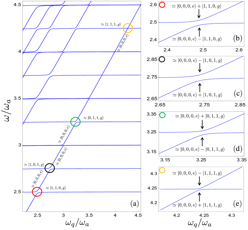
Figure 1: Energy levels and avoided level crossings for our system. (a) The relevant energy levels for our entanglement-generation protocol, normalized by $\omega_{a}$ and plotted as a function of the qubit frequency $\omega_{q}$. The transition frequencies of the three resonator modes are kept fixed. The plot is obtained by numerical diagonalization of the Hamiltonian in Eq. (5). All parameters used for the calculation are provided in the text. Panels (b), (c), (d), and (e) are zoom-ins of the areas marked by red, black, green, and yellow circles, respectively, in panel (a). These avoided level crossings, which occur when the qubit frequency equals the sum of some of the resonator-mode frequencies, indicate an effective coherent coupling between qubit and photonic states, which we can use for entanglement generation.

The lowest-energy horizontal line in the plot corresponds to the state with one photon each in the first two resonator modes, no photon in the third resonator mode, and the qubit in its ground state. We denote this state by

$$|\psi_{1},g\rangle=|1,1,0,g\rangle,$$ (9)

where on the right-hand side the first three entries are the number of photons in the resonator modes $a$, $b$, and $c$, respectively, and the last entry is the qubit state. To distinguish the qubit state from the photonic states, we hereafter denote the qubit ground state $|g\rangle$ and the excited state $|e\rangle$. Adopting this notation, the second, fourth and eighth horizontal lines correspond to, respectively,

$$|\psi_{2},g\rangle = |1,0,1,g\rangle,$$ (10)

$$|\psi_{3},g\rangle = |0,1,1,g\rangle,$$ (11)

$$|\psi_{4},g\rangle = |1,1,1,g\rangle.$$ (12)

We note that these eigenstates can differ from the bare eigenstates due to the dressing effects induced by the counter-rotating terms in the interaction part of the Hamiltonian in Eq. (5). These differences between bare and physical states occur, more or less, for all the energy eigenstates Di Stefano et al. (2017). For example, the bare state $|\psi_{1}\rangle|g\rangle$, describing the excitation of the first two resonator modes in the absence of interaction with the qubit, differs from the dressed state $|\psi_{1},g\rangle$ corresponding to the excitation of the first two physical resonator modes in the presence of interaction with the qubit. A signature of this dressing is the slight difference between the sum of the bare frequencies $\omega_{a}+\omega_{b}=2.5\omega_{a}$ and the lowest horizontal energy level ($\omega\approx 2.5\omega_{a}$) displayed in Fig. 1(a).

As $\omega_{\rm q}$ increases in Fig. 1(a), the energy level associated with the state

$$|\psi_{0},e\rangle=|0,0,0,e\rangle$$ (13)

rises to meet the energy levels corresponding to, from left to right, $|\psi_{1},g\rangle$, $|\psi_{2},g\rangle$, $|\psi_{3},g\rangle$ and $|\psi_{4},g\rangle$. The result is several avoided level crossings, marked by colored circles in the plot.

II.3.1 Second-order processes: Bell states

In Figs. 1(b)-(d), we show enlarged views of the regions marked by the red, black, and green circles in Fig. 1(a). These avoided level crossings arise due to coherent coupling between the state $|\psi_{0},e\rangle$ and the states $|\psi_{1},g\rangle$, $|\psi_{2},g\rangle$, and $|\psi_{3},g\rangle$, respectively, and occur at the points where the qubit frequency equals the sum of two of the resonator-mode frequencies. Explicitly, we have the resonance conditions

$$\omega_{q}\simeq\omega_{a}+\omega_{b}$$ (14)

in Fig. 1(b),

$$\omega_{q}\simeq\omega_{a}+\omega_{c}$$ (15)

in Fig. 1(c), and

$$\omega_{\rm q}\simeq\omega_{\rm b}+\omega_{\rm c}$$ (16)

in Fig. 1(d).

The essential point for entanglement generation is that the coherent coupling makes it such that, when the level splitting of the avoided level crossing is at its minimum, the eigenstates of the system are symmetric and antisymmetric superpositions of the states $|\psi_{0},e\rangle$ and $|\psi_{n},g\rangle$ ($n=1,2,3$). This is confirmed by numerical calculations. Thus, if we first initialize the system in $|\psi_{0},e\rangle$, and then tune the qubit frequency such that $|\psi_{0},e\rangle$ becomes resonant with $|\psi_{n},g\rangle$ ($n=1,2,3$), we will observe Rabi oscillations back and forth between $|\psi_{0},e\rangle$ and $|\psi_{n},g\rangle$. By initializing the system in a superposition of $|\psi_{0},e\rangle$ and $|0,0,0,g\rangle$, this allows us to create Bell states for photons in two resonator modes, as explained further below in Sec. III.1.

The coherent coupling at the avoided level crossings is due to a second-order process involving both the longitudinal and transversal coupling terms in Eq. (5). A detailed illustration of this second-order process can be found in Appendix A. The minimum level splitting at the avoided level crossing is determined by $g_{\rm eff}^{\rm(B)}$, the strength of the effective coupling between the states $|\psi_{0},e\rangle$ and $|\psi_{n},g\rangle$ induced by the second-order process. This coupling strength also sets the timescale for the Rabi oscillations between these states, and thus also the timescale for the entanglement generation in our protocol.

A good approximation of the effective coupling strength can be calculated analytically using second-order perturbation theory, considering all possible paths between the initial state $|i\rangle\equiv|\psi_{0}\rangle|e\rangle$ and the final state $|f\rangle\equiv|\psi_{n}\rangle|g\rangle$ ($n=1,2,3$), or vice versa. The details of these calculations are presented in Appendix A. For $n=1$, the result is

$$g_{\rm eff}^{\rm(B)}=-\frac{g_{a}g_{b}\left(\omega_{a}+\omega_{b}\right)\sin 2\theta}{\omega_{a}\omega_{b}}.$$ (17)

This result illustrates why USC is required for our protocol to work well. Since the effective coupling is due to a second-order process, it scales as $g^{2}/\omega$, and would thus become prohibitively small if $g\ll\omega$.

Since the perturbation theory uses $g/\omega$ as its small parameter, and we want to increase $g/\omega$ to generate entanglement faster, we check numerically how well this analytical result for the effective coupling strength agrees with the true value. The result is plotted in Fig. 2. The plot shows $g_{\rm eff}^{(B)}$ as a function of $g/\omega_{a}$ for $g_{a}=g_{b}=g$ and $g_{c}=0$. The red curve is the analytical result from Eq. (17) and the black dots are the results from the numerical diagonalization of the Hamiltonian in Eq. (5). We see that the analytical result remains a very good approximation for normalized interaction strengths $g/\omega_{\rm a}\lesssim 0.2$.

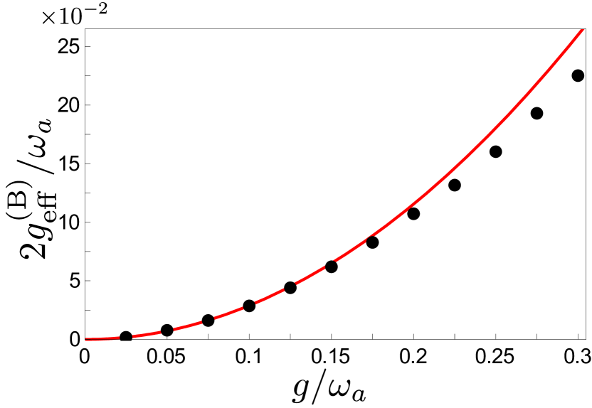
Figure 2: A comparison between the numerically calculated normalized effective coupling strength $g_{\rm eff}^{\rm(B)}/\omega_{\rm a}$ (black points) and the corresponding analytical result [Eq. (17)] from second-order perturbation theory (red curve). We used $g_{\rm a}=g_{\rm b}=g,g_{\rm c}=0$; all other parameters are the same as in Fig. 1.

II.3.2 Third-order process: GHZ state

Panel (e) in Fig. 1 shows an enlarged view of the region marked by a yellow circle in Fig. 1(a). This level crossing arises due to a third-order process creating a coherent coupling between the states $|\psi_{0},e\rangle$ and $|\psi_{4},g\rangle$, and occurs at the point where $\omega_{q}\simeq\omega_{a}+\omega_{b}+\omega_{c}$. As before, numerical calculations confirm that the eigenstates of the system at the point where the level splitting is at its minimum are the symmetric and antisymmetric superpositions of the states $|\psi_{0},e\rangle$ and $|\psi_{4},g\rangle$. This means that we can initialize the system in a superposition of $|\psi_{0},e\rangle$ and $|0,0,0,g\rangle$, and then transfer the qubit excitation to the three resonator modes to create a GHZ state for the photons in these modes, as explained in more detail below in Sec. III.1.

In this case, the level splitting is smaller than before, since the process is of a higher order than before. The third-order process responsible for the effective coupling does not require longitudinal coupling, since $|\psi_{0},e\rangle$ and $|\psi_{4},g\rangle$ have the same parity. A detailed illustration showing all transition paths that contribute to the effective coupling $g_{\rm eff}^{\rm(G)}$ is given in Appendix B. From third-order perturbation theory with $\theta=0$ in Eq. (5), we find

$$g_{\rm eff}^{\rm(G)}=-\frac{4g_{a}g_{b}g_{c}\left(\omega_{a}+\omega_{b}+\omega_{c}\right)}{\left(\omega_{a}+\omega_{b}\right)\left(\omega_{a}+\omega_{c}\right)\left(\omega_{b}+\omega_{c}\right)}.$$ (18)

The details of the calculations leading to this result are presented in Appendix B. As expected for a third-order process, the effective coupling scales as $g^{3}/\omega^{2}$, showing that being in the USC regime is more important for generation of GHZ states than for generation of Bell states.

Just as for $g_{\rm eff}^{\rm(B)}$ above, we compare the analytical result in Eq. (18) with full numerical calculations to see for which parameters the perturbation theory gives a good approximation of the true value for $g_{\rm eff}^{\rm(G)}$. The result of this comparison is plotted in Fig. 3. Just as in Fig. 2, the red curve is the analytical result and the black dots are the results from numerical diagonalization of the Hamiltonian. We note that the agreement between the perturbation-theory result and the correct value remains very good when $g/\omega_{\rm a}\lesssim 0.2$.

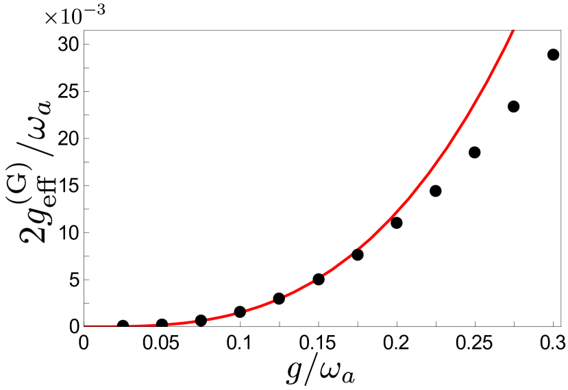
Figure 3: A comparison between the numerically calculated normalized effective coupling strength $g_{\rm eff}^{\rm(G)}/\omega_{\rm a}$ (black points) and the corresponding analytical result [Eq. (18)] from third-order perturbation theory (red curve). We used $g_{\rm a}=g_{\rm b}=g_{\rm c}=g$ and $\theta=0$; all other parameters are the same as in Fig. 1.

III Results

In this section, we first present the details of our entanglement-generation protocol. We then present results from numerical simulations of the protocol for both Bell and GHZ states, using experimentally feasible parameters and exploring the effect of losses on the fidelity of the protocol.

Table 1: The three Bell states whose generation we simulate in Fig. 4, the resonance conditions for their creation, and the qubit-photon coupling strengths used in the simulations.

Bell State	Resonance condition	Qubit-photon couplings
$B_{110}=\frac{1}{\sqrt{2}}\left(|\psi_{0}\rangle+e^{i\phi}|\psi_{1}\rangle\right)|g\rangle$	$\omega_{q}\simeq\omega_{a}+\omega_{b}$	$g_{a}=g_{b}=g,\>\>g_{c}=0$
$B_{101}=\frac{1}{\sqrt{2}}\left(|\psi_{0}\rangle+e^{i\phi}|\psi_{2}\rangle\right)|g\rangle$	$\omega_{q}\simeq\omega_{a}+\omega_{c}$	$g_{a}=g_{c}=g,\>\>g_{b}=0$
$B_{011}=\frac{1}{\sqrt{2}}\left(|\psi_{0}\rangle+e^{i\phi}|\psi_{3}\rangle\right)|g\rangle$	$\omega_{q}\simeq\omega_{b}+\omega_{c}$	$g_{c}=g_{b}=g,\>\>g_{a}=0$

III.1 Entanglement-generation protocol

The entanglement-generation protocol essentially consists of two steps. The steps in the protocol are the same for both Bell and GHZ states. The only difference between the two cases is which resonance condition is used; that determines whether photons from two or three resonator modes become entangled.

Step 1: We begin with the system in its ground state with the qubit frequency far detuned from any resonance with the resonator-mode frequencies (and their sums), i.e., in the state

$$|\psi_{0}\rangle|g\rangle=|0,0,0\rangle|g\rangle.$$ (19)

Then, we rotate the qubit state to a superposition state,

$$\frac{1}{\sqrt{2}}|\psi_{0}\rangle\left(|g\rangle+|e\rangle\right).$$ (20)

The idea of the protocol is to transfer this qubit superposition to several photons.

Step 2: We then tune the qubit frequency into resonance with the sum of the frequencies of the resonator modes that we wish to entangle. This will change the system state to

$$|\psi(t=0)\rangle=\frac{1}{\sqrt{2}}\left(|\psi_{0},g\rangle+|\psi_{0},e\rangle\right).$$ (21)

Let us assume that we have tuned the qubit frequency into resonance with the photonic state $|\psi_{n}\rangle$ ($n=1,2,3,4$), i.e., to one of the marked avoided level crossings in Fig. 1. As we showed in Sec. II.3, this will create an effective coupling of strength $g_{\rm eff}^{\rm(B/G)}$ between the states $|\psi_{0},e\rangle$ and $|\psi_{n},g\rangle$. The state $|\psi_{0},g\rangle$ is not affected. The system state will thus undergo Rabi oscillations and evolve in time as

$$|\psi(t)\rangle = \frac{1}{\sqrt{2}}\Big{[}|\psi_{0},g\rangle+\cos\left(g_{\rm eff}^{\rm(B/G)}t\right)|\psi_{0},e\rangle$$ (22)

$$-i\sin\left(g_{\rm eff}^{\rm(B/G)}t\right)|\psi_{n},g\rangle\Big{]}.$$

After a time $t=\pi/2g_{\rm eff}^{\rm(B/G)}$, we detune the qubit far from the resonance. This leaves the system in the state

$$\frac{1}{\sqrt{2}}\left(|\psi_{0}\rangle+e^{i\phi}|\psi_{n}\rangle\right)|g\rangle,$$ (23)

where $\phi\in\mathbb{R}$. This is an entangled state of photons in the resonator modes. The qubit is no longer entangled with the photons. For $n=1,2,3$, the entangled photonic state is a Bell state for the photons in resonator modes $a$ and $b$, $a$ and $c$, or $b$ and $c$, respectively. For $n=4$, the entangled photonic state is a GHZ state involving all three resonator modes. We note again that the case $n=4$ does not require the longitudinal coupling term in Eq. (5), since this process conserves the parity of the number of excitations in the system.

III.2 Numerical simulations for the Bell states

Here we simulate our protocol for Bell-state generation, taking into account losses. We do this by solving the master equation in Eq. (6). The results are presented in Fig. 4. We use the same parameters for the resonator-mode and qubit frequencies and coupling strength as in Fig. 1. To simplify the simulations, we start with the qubit already in a superposition state and tuned to the desired resonance, but with all couplings turned off. At the time marked by the vertical grey dashed line in panels (a)-(c) in Fig. 4, we turn on the coupling to the two resonator modes that we wish to create a Bell state for, i.e., at this point, we start from the state in Eq. (21). After a time $t\approx\pi/2g_{\rm eff}^{\rm(B)}$, we detune the qubit frequency from the resonance [pink curve in panels (a)-(c) in Fig. 4]. For clarity, we list in Table 1 the three Bell states together with the corresponding resonance conditions and couplings turned on in the simulations.

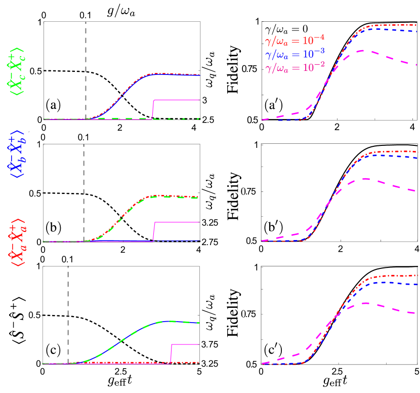
Figure 4: Simulations of the protocol for Bell-state generation under the influence of decoherence. The left panels show the number of excitations in resonator mode $a$, $\left\langle\hat{X}_{a}^{-}\hat{X}_{a}^{+}\right\rangle$ (red dashed-dotted curves), in resonator mode $b$, $\left\langle\hat{X}_{b}^{-}\hat{X}_{b}^{+}\right\rangle$ (blue solid curves), in resonator mode $c$, $\left\langle\hat{X}_{c}^{-}\hat{X}_{c}^{+}\right\rangle$ (green large-dashed curve), and in the qubit, $\left\langle\hat{S}^{-}\hat{S}^{+}\right\rangle$ (black dashed curve). These are plotted as a function of time during the creation of the Bell states (a) $B_{110}$, (b) $B_{101}$, and (c) $B_{011}$ (see Table 1 for definition of this notation). In panels (a)-(c), the vertical grey dashed lines indicate when the coupling between the qubit (which starts in a superposition state) and the relevant resonator modes is turned on. The pink solid curve shows how the qubit frequency $\omega_{q}$ is tuned during the protocol. This is given by the smoothed step function $\omega_{q}(t)=\omega_{q,i}+\delta\omega_{q}\left\{\sin^{2}\left[A(t-t_{i})\right]\Theta(t-t_{i})+\sin^{2}\left[A(t-t_{f})\right]\Theta(t-t_{f})\right\}$, where $\omega_{q,i}$ is the initial qubit frequency, $\delta\omega_{q}$ is the change of the qubit frequency, $\Theta$ is the Heaviside step function, $t_{i}$ is the time when the qubit frequency starts to change, $t_{f}=t_{i}+\pi/(2A)$, and $A$ is a frequency setting the smoothness. Panels (a’)-(c’) are plots of the fidelities for producing the desired entangled states from panels (a)-(c) given different decoherence rates. All parameters for the simulations are given in the text.

In panels (a)-(c) in Fig. 4, we show the time evolution for the qubit and resonator-mode populations during the whole protocol. Note that the populations must be calculated using the dressed operators given in Eq. (8). Panel (a) is for the generation of the Bell state with photons in modes $a$ and $b$, panel (b) is the result for photons in modes $a$ and $c$, and panel (c) is for the case with photons in modes $b$ and $c$. In all these panels, we use the decoherence parameters $\gamma=10^{-3}\omega_{\rm a}$ and $\kappa_{\rm a}=\kappa_{\rm b}=\kappa_{\rm c}=\gamma/2$.

To test the robustness of our Bell-state-generation protocol, we repeated these simulations for different values of the decoherence rate $\gamma$ and calculated the fidelity $\mathcal{F}=\sqrt{\langle\psi|\rho(t)|\psi\rangle}$ for the desired entangled state $|\psi\rangle$. The results are shown in panels (a’)-(c’) in Fig. 4. We observe that the protocol works well as long as $\gamma/\omega_{a}\lesssim 10^{-3}$, producing entangled states with a fidelity of 90% or above. For larger decoherence rates, the fidelity becomes markedly lower, since we then enter a regime where $\gamma$ starts to become comparable to $g_{\rm eff}^{\rm(B)}$.

III.3 Numerical simulations for the GHZ state

We now perform numerical simulations also for the GHZ-state-generation protocol with losses included. We do this in the same way as for the Bell states in Sec. III.2. The results are plotted in Fig. 5. The resonator-mode frequencies are the same as in the previous plots, while the qubit frequency is tuned to the resonance for the GHZ state, $\omega_{\rm q}\simeq\omega_{\rm a}+\omega_{\rm b}+\omega_{\rm c}$. Since a longitudinal coupling is not required to generate the GHZ state, we set $\theta=0$. We use a slightly higher coupling strength, $g=0.12\omega_{\rm a}$, since $g_{\rm eff}^{\rm(G)}$ otherwise would be much weaker than $g_{\rm eff}^{\rm(B)}$. When the coupling is turned on, marked by the vertical dashed grey line in panel (a), we set $g_{a}=g_{b}=g_{c}=g$. Decoherence is included with qubit and resonator losses at the same levels as in Fig. 4.

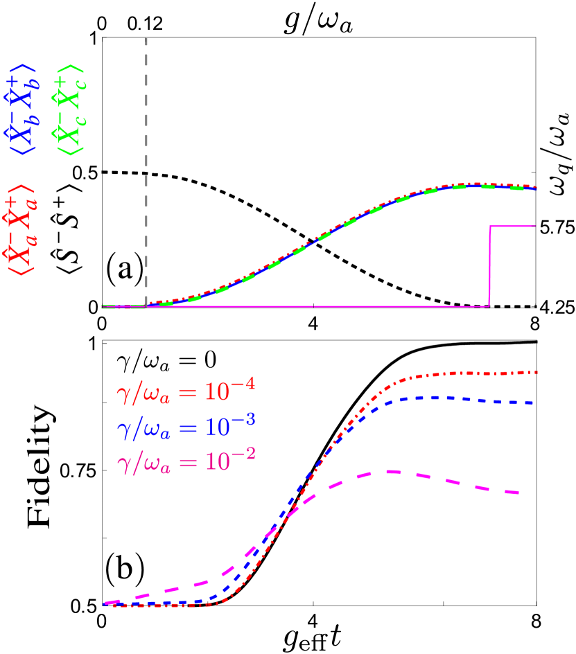
Figure 5: Simulations of the protocol for GHZ-state generation under the influence of decoherence. (a) The number of excitations in resonator mode $a$, $\left\langle\hat{X}_{a}^{-}\hat{X}_{a}^{+}\right\rangle$ (red dashed-dotted curves), in resonator mode $b$, $\left\langle\hat{X}_{b}^{-}\hat{X}_{b}^{+}\right\rangle$ (blue solid curves), in resonator mode $c$, $\left\langle\hat{X}_{c}^{-}\hat{X}_{c}^{+}\right\rangle$ (green large-dashed curve), and in the qubit, $\left\langle\hat{S}^{-}\hat{S}^{+}\right\rangle$ (black dashed curve). These are plotted as a function of time during the creation of the GHZ state. The vertical grey dashed line indicates when the coupling between the qubit (which starts in a superposition state) and the resonator modes is turned on. The pink solid curve shows how the qubit frequency $\omega_{q}$ is tuned during the protocol; the form of this curve is the same as in Fig. 4. (b) Fidelities for producing the desired GHZ state from panel (a) given different decoherence rates. All parameters for the simulations are given in the text.

In panel (a) in Fig. 5, we show the time evolution for the qubit and resonator-mode populations during the whole protocol. In panel (b), we plot the fidelity for the GHZ state as a function of time for different decoherence rates. Again, the protocol works well when $\gamma/\omega_{a}\lesssim 10^{-3}$; for larger decoherence rates, the fidelity declines since $\gamma$ starts to become comparable to $g_{\rm eff}^{\rm(G)}$.

III.4 Experimental feasibility

Here we briefly comment on the experimental feasibility of our entanglement-generation protocol. As described in the introduction, circuit-QED systems are the only experimental setups so far to demonstrate USC with single atoms. We therefore limit the discussion here to parameters in circuit-QED experiments, although our protocol may become possible to implement in other systems in the future.

As we saw in Secs. III.2 and III.3, the essential requirement for generating entangled photonic states with high fidelity using our protocol is that the effective coupling $g_{\rm eff}^{\rm(B/G)}$ is clearly larger than the decoherence rates in the system. Since circuit-QED systems can reach the USC regime $g/\omega>0.1$, they can surely realize $g_{\rm eff}^{\rm(B/G)}/\omega\sim 10^{-3}-10^{-2}$ [compare Eqs. (17) and (18)]. When it comes to decoherence rates, flux qubits have demonstrated relaxation rates as low as $\gamma/\omega\sim 10^{-6}$ Stern et al. (2014); Orgiazzi et al. (2016); Yan et al. (2016). Similarly, superconducting transmission-line resonators with relaxation rates on the order of $\kappa/\omega\sim 10^{-6}$ Megrant et al. (2012) have been fabricated; three-dimensional resonators for circuit QED can even reach $\kappa/\omega\sim 10^{-8}$ Reagor et al. (2013). We therefore expect that our scheme can create photonic Bell and GHZ states with high fidelity using existing technology.

IV Conclusion and outlook

We have presented a simple protocol for the deterministic preparation of photonic Bell and GHZ states. We do this in a setup consisting of three resonator modes, all of different frequencies, coupled to a single qubit. The protocol relies on this coupling between light and matter being ultrastrong, which enables higher-order processes that do not conserve the number of excitations in the system. Using this property, a superposition state prepared for the qubit can be transferred to multiple photons in the resonator modes. Our protocol is versatile, since the same setup, and the same steps, can be used to generate all these maximally entangled states. The only thing that changes depending on which entangled state we wish to create, is which frequency we tune the qubit to. The resonance condition we need is that the qubit frequency equals the sum of the frequencies of the resonator modes that are to be entangled.

We have shown that our protocol is ready to be implemented in circuit-QED experiments using state-of-the-art technology. Seeing as USC is being achieved in more and more experimental systems, we expect that our protocol will be useful in other systems as well in the future. We believe that our protocol could be useful as a method to distribute entanglement at a node in a quantum network.

It is clear that our protocol can be extended to create entangled states involving four or more photons of different frequencies. This simply requires adding more resonator modes and tuning the qubit frequency to equal the sum of these resonator-mode frequencies. However, the effective coupling strength, which determines how fast we can transfer the superposition state from the qubit to the photons, will become weaker the more resonator modes are involved. This is because populating more photonic modes requires a process of higher order, and the effective coupling scales as $\left(g/\omega\right)^{n-1}$ for an $n$th-order process Kockum et al. (2017a). Such a weak effective coupling will only give an entangled state with low fidelity unless the decoherence rates in the system are even lower.

It is also interesting to think about whether our protocol can be extended to create other types of entangled states. For three photons, the GHZ and W states are the only two distinct types of maximally entangled states Dür et al. (2000). However, it is not clear how the idea of our protocol could be used to create a W state for photons of different frequencies, since this requires creating a superposition of three different states, all with different energies.

Appendix A Analytical calculation of the effective coupling for generating Bell states

In this appendix, we calculate the effective coupling rates $g_{\rm eff}^{\rm(B)}$ for the processes that we use to generate entangled Bell states between photons in two resonator modes.

A.1 System

For the Bell-state-generation, we only need to consider two resonator modes, with transition frequencies $\omega_{a}$ and $\omega_{b}$, respectively, both ultrastrongly coupled to a qubit with transition frequency $\omega_{q}$. The relevant system Hamiltonian is obtained from Eq. (5), neglecting the third resonator mode:

$$\hat{H} = \omega_{a}\hat{a}^{\dagger}\hat{a}+\omega_{b}\hat{b}^{\dagger}\hat{b}+\frac{\omega_{q}}{2}\hat{\sigma}_{z}$$

$$+\left[g_{a}\left(\hat{a}^{\dagger}+\hat{a}\right)+g_{b}\left(\hat{b}^{\dagger}+\hat{b}\right)\right]\left(\hat{\sigma}_{x}\cos\theta+\hat{\sigma}_{z}\sin\theta\right),$$

where $\hat{a}$ ($\hat{a}^{\dagger}$) is the annihilation (creation) operator of the first resonator mode, $\hat{b}$ ($\hat{b}^{\dagger}$) is the annihilation (creation) operator of the second resonator mode, $\hat{\sigma}_{z}$ and $\hat{\sigma}_{x}$ are the Pauli matrices for the qubit, $g_{a}$ ($g_{b}$) is the coupling between the first (second) resonator and the qubit, and $\theta$ is an angle parameterizing the amount of longitudinal and transversal coupling. The longitudinal coupling term in this generalized quantum Rabi Hamiltonian is necessary for the process we have in mind, since that process neither conserves the number of excitations in the system nor their parity.

A.2 Transition paths and perturbation theory

To generate the Bell state, we need a transition between the states $|0,0,e\rangle$ and $|1,1,g\rangle$. These two states are connected via a second-order process. There are four paths connecting the states to this order, as shown in Fig. 6.

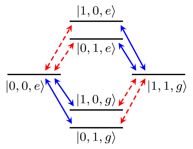
Figure 6: The four second-order paths connecting the states $|0,0,e\rangle$ and $|1,1,g\rangle$. Transitions that do not conserve the number of excitations in the system are marked by dashed lines while transitions that conserve the number of excitations are marked by solid lines. Red lines mark transitions mediated by the $\hat{\sigma}_{z}$ part of the coupling and blue lines mark transitions mediated by the $\hat{\sigma}_{x}$ part of the coupling. To set the energy levels, we have used the parameter values $\omega_{q}=2.5\omega_{b}$ and $\omega_{a}=1.5\omega_{b}$.

We can treat the interaction part of the Hamiltonian in Eq. (LABEL:eq:HBell),

$$\hat{V}=\left[g_{\rm a}\left(\hat{a}^{\dagger}+\hat{a}\right)+g_{\rm b}\left(\hat{b}^{\dagger}+\hat{b}\right)\right]\left(\hat{\sigma}_{x}\cos\theta+\hat{\sigma}_{z}\sin\theta\right),$$ (25)

as a perturbation, provided that $g_{a},g_{b}\ll\omega_{a},\omega_{b},\omega_{q}$. Writing

$$V_{nm}=\langle n|\hat{V}|m\rangle,$$ (26)

from second-order perturbation theory we have that the effective coupling between the initial state $|i\rangle=|0,0,e\rangle$ and the final state $|f\rangle=|1,1,g\rangle$ is given by

$$g_{\rm eff}=\sum_{n}\frac{V_{fn}V_{ni}}{\left(E_{i}-E_{n}\right)},$$ (27)

where the sum goes over all paths shown in Fig. 6. Note that $E_{i}=\frac{1}{2}\omega_{q}=E_{f}=\omega_{a}+\omega_{b}-\frac{1}{2}\omega_{q}$ when we are at the resonance $\omega_{q}=\omega_{a}+\omega_{b}$, which is the case we consider here. The contributions from the four transition paths add up to

$$g_{\rm eff}^{\rm(B)} = -g_{a}g_{b}\sin\theta\cos\theta\left(\frac{1}{\omega_{a}}+\frac{1}{\omega_{b}}+\frac{1}{\omega_{q}-\omega_{a}}+\frac{1}{\omega_{q}-\omega_{b}}\right)$$ (28)

$$= -g_{a}g_{b}\sin 2\theta\left(\frac{1}{\omega_{a}}+\frac{1}{\omega_{b}}\right)$$

$$= -\frac{g_{a}g_{b}\left(\omega_{a}+\omega_{b}\right)\sin 2\theta}{\omega_{a}\omega_{b}}.$$

Looking at the denominator of Eq. (28), we see that $g_{\rm eff}\to\infty$ when $\omega_{a}\to 0$ or $\omega_{a}\to 0$, i.e., when the qubit becomes resonant with one of resonator modes. The perturbation theory is not valid around those points, nor is it valid when $\omega_{a}\approx\omega_{b}$, since the states $|2,0,g\rangle$ and $|0,2,g\rangle$ then would have approximately the same energy as the initial and final states in the process we considered here. For similar reasons, we also want to avoid that $\omega_{q}=n\omega_{a}$, $\omega_{q}=m\omega_{b}$, and $\omega_{a}=k\omega_{b}$, where $n,m,k$ are integers. Finally, we note that since the effective coupling is proportional to $\sin 2\theta$, it will reach its maximum value when $\theta=\pi/4+n\pi/2$.

Appendix B Analytical calculation of the effective coupling for generating GHZ states

In this appendix, we calculate the effective coupling rates $g_{\rm eff}^{\rm(G)}$ for the process that we use to generate an entangled GHZ state between photons in three resonator modes.

B.1 System

Our system now consists of three resonator modes, with transition frequencies $\omega_{a}$, $\omega_{b}$, and $\omega_{c}$, respectively, all ultrastrongly coupled to a qubit with transition frequency $\omega_{q}$. The relevant system Hamiltonian is obtained from Eq. (5) with $\theta=0$:

$$\hat{H} = \omega_{\rm a}\hat{a}^{\dagger}\hat{a}+\omega_{\rm b}\hat{b}^{\dagger}\hat{b}+\omega_{\rm c}\hat{c}^{\dagger}\hat{c}+\frac{\omega_{\rm q}}{2}\hat{\sigma}_{z}$$ (29)

$$+\hat{\sigma}_{x}\left[g_{\rm a}\left(\hat{a}^{\dagger}+\hat{a}\right)+g_{\rm b}\left(\hat{b}^{\dagger}+\hat{b}\right)+g_{\rm c}\left(\hat{c}^{\dagger}+\hat{c}\right)\right],\quad$$

where $\hat{a}$ ($\hat{a}^{\dagger}$) is the annihilation (creation) operator of the first resonator mode, $\hat{b}$ ($\hat{b}^{\dagger}$) is the annihilation (creation) operator of the second resonator mode, $\hat{c}$ ($\hat{c}^{\dagger}$) is the annihilation (creation) operator of the third resonator mode, $\hat{\sigma}_{z}$ and $\hat{\sigma}_{x}$ are the Pauli matrices for the qubit, and $g_{j}$ is the coupling between resonator $j$ and the qubit. For this process, the standard quantum Rabi Hamiltonian with only transversal coupling ($\theta=0$), expanded to include multiple resonator modes, is sufficient, since the process needed for the GHZ-state generation conserves the parity of the number of excitations.

B.2 Transition paths and perturbation theory

To generate the GHZ state, we need a transition between the states $|0,0,0,e\rangle$ and $|1,1,1,g\rangle$. These two states are connected via a third-order process. There are six paths connecting the states to this order, as shown in Fig. 7.

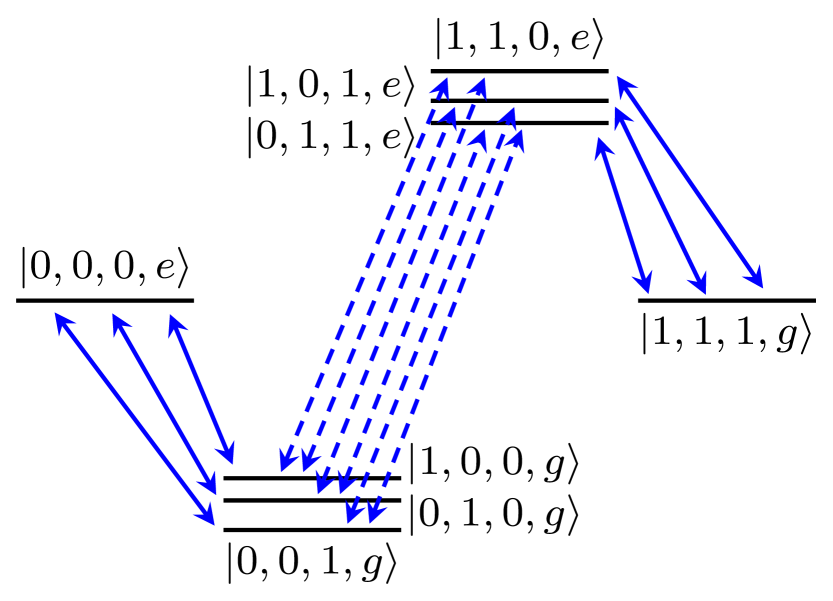
Figure 7: The six third-order paths connecting the states $|0,0,0,e\rangle$ and $|1,1,1,g\rangle$. Transitions that do not conserve the number of excitations in the system are marked by dashed lines while transitions that conserve the number of excitations are marked by solid lines. To set the energy levels, we have used the parameter values $\omega_{q}=4.1\omega_{c}$, $\omega_{a}=1.7\omega_{c}$, and $\omega_{b}=1.4\omega_{c}$.

We can treat the interaction part of the Hamiltonian in Eq. (29),

$$\hat{V}=\hat{\sigma}_{x}\left[g_{\rm a}\left(\hat{a}^{\dagger}+\hat{a}\right)+g_{\rm b}\left(\hat{b}^{\dagger}+\hat{b}\right)+g_{\rm c}\left(\hat{c}^{\dagger}+\hat{c}\right)\right],$$ (30)

as a perturbation, provided that $g_{a},g_{b},g_{c}\ll\omega_{a},\omega_{b},\omega_{c},\omega_{q}$. From third-order perturbation theory, we have that the effective coupling between the initial state $|i\rangle=|0,0,0,e\rangle$ and the final state $|f\rangle=|1,1,1,g\rangle$ is given by

$$g_{\rm eff}=\sum_{n,m}\frac{V_{fn}V_{nm}V_{mi}}{\left(E_{i}-E_{n}\right)\left(E_{i}-E_{m}\right)},$$ (31)

where the sum goes over all paths shown in Fig. 7. Note that $E_{i}=\frac{1}{2}\omega_{q}=E_{f}=\omega_{a}+\omega_{b}+\omega_{c}-\frac{1}{2}\omega_{q}$ when we are at the resonance $\omega_{q}=\omega_{a}+\omega_{b}+\omega_{c}$, which is the case we consider here. The contributions from the six transition paths add up to

$$g_{\rm eff}^{(G)} = -g_{a}g_{b}g_{c}\Bigg{[}\frac{1}{\left(\omega_{a}+\omega_{b}\right)\left(\omega_{q}-\omega_{a}\right)}+\frac{1}{\left(\omega_{a}+\omega_{b}\right)\left(\omega_{q}-\omega_{b}\right)}+\frac{1}{\left(\omega_{a}+\omega_{c}\right)\left(\omega_{q}-\omega_{a}\right)}$$ (32)

$$+\frac{1}{\left(\omega_{a}+\omega_{c}\right)\left(\omega_{q}-\omega_{c}\right)}+\frac{1}{\left(\omega_{b}+\omega_{c}\right)\left(\omega_{q}-\omega_{b}\right)}+\frac{1}{\left(\omega_{b}+\omega_{c}\right)\left(\omega_{q}-\omega_{c}\right)}\Bigg{]}$$

$$= -2g_{a}g_{b}g_{c}\left[\frac{1}{\left(\omega_{a}+\omega_{b}\right)\left(\omega_{b}+\omega_{c}\right)}+\frac{1}{\left(\omega_{a}+\omega_{c}\right)\left(\omega_{b}+\omega_{c}\right)}+\frac{1}{\left(\omega_{a}+\omega_{b}\right)\left(\omega_{a}+\omega_{c}\right)}\right]$$

$$= -\frac{4g_{a}g_{b}g_{c}\left(\omega_{a}+\omega_{b}+\omega_{c}\right)}{\left(\omega_{a}+\omega_{b}\right)\left(\omega_{a}+\omega_{c}\right)\left(\omega_{b}+\omega_{c}\right)}.$$

Looking at the denominator of Eq. (32), we see that $g_{\rm eff}\to\infty$ if two of the three resonator frequencies go to zero, i.e., when the qubit becomes resonant with one of resonator modes. The perturbation theory is not valid around those points. Nor is it valid when additional states, containing two or more photons in one of the resonator modes, have approximately the same energy as the initial and final states in the process we considered here.

References

- Horodecki et al. (2009) R. Horodecki, P. Horodecki, M. Horodecki, and K. Horodecki, “Quantum entanglement,” Rev. Mod. Phys. 81, 865 (2009), arXiv:0702225 [quant-ph] .
- Gisin and Thew (2007) N. Gisin and R. Thew, “Quantum communication,” Nat. Photonics 1, 165 (2007), arXiv:0703255 [quant-ph] .
- Nielsen and Chuang (2000) M. A. Nielsen and I. L. Chuang, Quantum Computation and Quantum Information (Cambridge University Press, 2000).
- Ladd et al. (2010) T. D. Ladd, F. Jelezko, R. Laflamme, Y. Nakamura, C. Monroe, and J. L. O’Brien, “Quantum computers,” Nature 464, 45 (2010), arXiv:1009.2267 .
- Buluta et al. (2011) I. Buluta, S. Ashhab, and F. Nori, “Natural and artificial atoms for quantum computation,” Reports Prog. Phys. 74, 104401 (2011), arXiv:1002.1871 .
- Wendin (2017) G. Wendin, “Quantum information processing with superconducting circuits: a review,” Reports Prog. Phys. 80, 106001 (2017), arXiv:1610.02208 .
- Gu et al. (2017) X. Gu, A. F. Kockum, A. Miranowicz, Y.-X. Liu, and F. Nori, “Microwave photonics with superconducting quantum circuits,” Phys. Rep. 718-719, 1–102 (2017), arXiv:1707.02046 .
- Flamini et al. (2018) F. Flamini, N. Spagnolo, and F. Sciarrino, “Photonic quantum information processing: a review,” (2018), arXiv:1803.02790 .
- Bennett et al. (1993) C. H. Bennett, G. Brassard, C. Crépeau, R. Jozsa, A. Peres, and W. K. Wootters, “Teleporting an unknown quantum state via dual classical and Einstein-Podolsky-Rosen channels,” Phys. Rev. Lett. 70, 1895 (1993).
- Ekert (1991) A. K. Ekert, “Quantum cryptography based on Bell’s theorem,” Phys. Rev. Lett. 67, 661 (1991).
- Hillery et al. (1999) M. Hillery, V. Bužek, and A. Berthiaume, “Quantum secret sharing,” Phys. Rev. A 59, 1829 (1999), arXiv:9806063 [quant-ph] .
- Long and Liu (2002) G. L. Long and X. S. Liu, “Theoretically efficient high-capacity quantum-key-distribution scheme,” Phys. Rev. A 65, 032302 (2002), arXiv:0012056 [quant-ph] .
- Deng et al. (2003) F.-G. Deng, G. L. Long, and X.-S. Liu, “Two-step quantum direct communication protocol using the Einstein-Podolsky-Rosen pair block,” Phys. Rev. A 68, 042317 (2003), arXiv:0308173 [quant-ph] .
- Briegel et al. (1998) H.-J. Briegel, W. Dür, J. I. Cirac, and P. Zoller, “Quantum Repeaters: The Role of Imperfect Local Operations in Quantum Communication,” Phys. Rev. Lett. 81, 5932 (1998), arXiv:9803056v1 [quant-ph] .
- Li and Deng (2015) T. Li and F.-G. Deng, “Heralded high-efficiency quantum repeater with atomic ensembles assisted by faithful single-photon transmission,” Sci. Rep. 5, 15610 (2015), arXiv:1511.00095 .
- Greenberger et al. (1989) D. M. Greenberger, M. A. Horne, and A. Zeilinger, “Going Beyond Bell’s Theorem,” in Bell’s Theorem, Quantum Theory and Conceptions of the Universe, edited by M. Kafatos (Springer Netherlands, Dordrecht, 1989) p. 69, arXiv:0712.0921 .
- Bouwmeester et al. (1999) D. Bouwmeester, J.-W. Pan, M. Daniell, H. Weinfurter, and A. Zeilinger, “Observation of Three-Photon Greenberger-Horne-Zeilinger Entanglement,” Phys. Rev. Lett. 82, 1345 (1999).
- Dür et al. (2000) W. Dür, G. Vidal, and J. I. Cirac, “Three qubits can be entangled in two inequivalent ways,” Phys. Rev. A 62, 062314 (2000), arXiv:0005115 [quant-ph] .
- Aspect et al. (1982) A. Aspect, J. Dalibard, and G. Roger, “Experimental Test of Bell’s Inequalities Using Time- Varying Analyzers,” Phys. Rev. Lett. 49, 1804 (1982).
- Weihs et al. (1998) G. Weihs, T. Jennewein, C. Simon, H. Weinfurter, and A. Zeilinger, “Violation of Bell’s Inequality under Strict Einstein Locality Conditions,” Phys. Rev. Lett. 81, 5039 (1998), arXiv:9810080 [quant-ph] .
- Mølmer and Sørensen (1999) K. Mølmer and A. Sørensen, “Multiparticle Entanglement of Hot Trapped Ions,” Phys. Rev. Lett. 82, 1835 (1999), arXiv:9810040 [quant-ph] .
- Pan et al. (2000) J.-W. Pan, D. Bouwmeester, M. Daniell, H. Weinfurter, and A. Zeilinger, “Experimental test of quantum nonlocality in three-photon Greenberger‚ÄìHorne‚ÄìZeilinger entanglement,” Nature 403, 515 (2000).
- Zhao et al. (2003) Z. Zhao, T. Yang, Y.-A. Chen, A.-N. Zhang, M. Żukowski, and J.-W. Pan, “Experimental Violation of Local Realism by Four-Photon Greenberger-Horne-Zeilinger Entanglement,” Phys. Rev. Lett. 91, 180401 (2003), arXiv:0302137 [quant-ph] .
- Wei et al. (2006) L. F. Wei, Y.-X. Liu, and F. Nori, “Generation and Control of Greenberger-Horne-Zeilinger Entanglement in Superconducting Circuits,” Phys. Rev. Lett. 96, 246803 (2006), arXiv:0510169 [quant-ph] .
- Steffen et al. (2006) M. Steffen, M. Ansmann, R. C. Bialczak, N. Katz, E. Lucero, R. McDermott, M. Neeley, E. M. Weig, A. N. Cleland, and J. M. Martinis, “Measurement of the Entanglement of Two Superconducting Qubits via State Tomography,” Science 313, 1423 (2006).
- Coelho et al. (2009) A. S. Coelho, F. A. S. Barbosa, K. N. Cassemiro, A. S. Villar, M. Martinelli, and P. Nussenzveig, “Three-Color Entanglement,” Science 326, 823 (2009).
- Bishop et al. (2009) L. S. Bishop, L. Tornberg, D. Price, E. Ginossar, A. Nunnenkamp, A. A. Houck, J. M. Gambetta, J. Koch, G. Johansson, S. M. Girvin, and R. J. Schoelkopf, “Proposal for generating and detecting multi-qubit GHZ states in circuit QED,” New J. Phys. 11, 073040 (2009), arXiv:0902.0324 .
- Zhang et al. (2009) J. Zhang, Y.-X. Liu, C.-W. Li, T.-J. Tarn, and F. Nori, “Generating stationary entangled states in superconducting qubits,” Phys. Rev. A 79, 052308 (2009), arXiv:0808.0395 .
- DiCarlo et al. (2010) L. DiCarlo, M. D. Reed, L. Sun, B. R. Johnson, J. M. Chow, J. M. Gambetta, L. Frunzio, S. M. Girvin, M. H. Devoret, and R. J. Schoelkopf, “Preparation and measurement of three-qubit entanglement in a superconducting circuit,” Nature 467, 574 (2010).
- Wang et al. (2010) Y.-D. Wang, S. Chesi, D. Loss, and C. Bruder, “One-step multiqubit Greenberger-Horne-Zeilinger state generation in a circuit QED system,” Phys. Rev. B 81, 104524 (2010), arXiv:0911.1396 .
- Hasegawa et al. (2010) Y. Hasegawa, R. Loidl, G. Badurek, K. Durstberger-Rennhofer, S. Sponar, and H. Rauch, “Engineering of triply entangled states in a single-neutron system,” Phys. Rev. A 81, 032121 (2010), arXiv:0908.0623 .
- Pan et al. (2012) J.-W. Pan, Z.-B. Chen, C.-Y. Lu, H. Weinfurter, A. Zeilinger, and M. Żukowski, “Multiphoton entanglement and interferometry,” Rev. Mod. Phys. 84, 777 (2012), arXiv:0805.2853 .
- Ristè et al. (2013) D. Ristè, M. Dukalski, C. A. Watson, G. de Lange, M. J. Tiggelman, Y. M. Blanter, K. W. Lehnert, R. N. Schouten, and L. DiCarlo, “Deterministic entanglement of superconducting qubits by parity measurement and feedback,” Nature 502, 350 (2013), arXiv:1306.4002 .
- Su et al. (2014) Q.-P. Su, C.-P. Yang, and S.-B. Zheng, “Fast and simple scheme for generating NOON states of photons in circuit QED,” Sci. Rep. 4, 3898 (2014), arXiv:1308.1793 .
- Johansson et al. (2014) J. R. Johansson, N. Lambert, I. Mahboob, H. Yamaguchi, and F. Nori, “Entangled-state generation and Bell inequality violations in nanomechanical resonators,” Phys. Rev. B 90, 174307 (2014), arXiv:1402.4900 .
- Zang et al. (2015) X.-P. Zang, M. Yang, F. Ozaydin, W. Song, and Z.-L. Cao, “Generating multi-atom entangled W states via light-matter interface based fusion mechanism,” Sci. Rep. 5, 16245 (2015), arXiv:1602.05046 .
- Yang et al. (2016) C.-P. Yang, Q.-P. Su, S.-B. Zheng, and F. Nori, “Entangling superconducting qubits in a multi-cavity system,” New J. Phys. 18, 013025 (2016), arXiv:1506.06108 .
- Kang et al. (2016) Y.-H. Kang, Y.-H. Chen, Q.-C. Wu, B.-H. Huang, J. Song, and Y. Xia, “Fast generation of W states of superconducting qubits with multiple Schrödinger dynamics,” Sci. Rep. 6, 36737 (2016).
- Tashima et al. (2016) T. Tashima, M. S. Tame, S. K. Özdemir, F. Nori, M. Koashi, and H. Weinfurter, “Photonic multipartite entanglement conversion using nonlocal operations,” Phys. Rev. A 94, 052309 (2016), arXiv:1610.04503 .
- Zhang et al. (2016) C. Zhang, Y.-F. Huang, C. Zhang, J. Wang, B.-H. Liu, C.-F. Li, and G.-C. Guo, “Generation and applications of an ultrahigh-fidelity four-photon Greenberger-Horne-Zeilinger state,” Opt. Express 24, 27059 (2016), arXiv:1702.04130 .
- Ritboon et al. (2017) A. Ritboon, S. Croke, and S. M. Barnett, “Proposed optical realisation of a two photon, four-qubit entangled state,” J. Opt. 19, 075201 (2017), arXiv:1703.01965 .
- Erhard et al. (2017) M. Erhard, M. Malik, M. Krenn, and A. Zeilinger, “Experimental GHZ Entanglement beyond Qubits,” (2017), arXiv:1708.03881 .
- Qin et al. (2018) W. Qin, A. Miranowicz, P.-B. Li, X.-Y. Lü, J.-Q. You, and F. Nori, “Exponentially Enhanced Light-Matter Interaction, Cooperativities, and Steady-State Entanglement Using Parametric Amplification,” Phys. Rev. Lett. 120, 093601 (2018), arXiv:1709.09555 .
- Cruz et al. (2018) D. Cruz, R. Fournier, F. Gremion, A. Jeannerot, K. Komagata, T. Tosic, J. Thiesbrummel, C. L. Chan, N. Macris, M.-A. Dupertuis, and C. Javerzac-Galy, “Efficient quantum algorithms for GHZ and W states, and implementation on the IBM quantum computer,” (2018), arXiv:1807.05572 .
- Monz et al. (2011) T. Monz, P. Schindler, J. T. Barreiro, M. Chwalla, D. Nigg, W. A. Coish, M. Harlander, W. Hänsel, M. Hennrich, and R. Blatt, “14-Qubit Entanglement: Creation and Coherence,” Phys. Rev. Lett. 106, 130506 (2011), arXiv:1009.6126 .
- Wang et al. (2016) X.-L. Wang, L.-K. Chen, W. Li, H.-L. Huang, C. Liu, C. Chen, Y.-H. Luo, Z.-E. Su, D. Wu, Z.-D. Li, H. Lu, Y. Hu, X. Jiang, C.-Z. Peng, L. Li, N.-L. Liu, Y.-A. Chen, C.-Y. Lu, and J.-W. Pan, “Experimental Ten-Photon Entanglement,” Phys. Rev. Lett. 117, 210502 (2016), arXiv:1605.08547 .
- Hou et al. (2016) Z. Hou, H.-S. Zhong, Y. Tian, D. Dong, B. Qi, L. Li, Y. Wang, F. Nori, G.-Y. Xiang, C.-F. Li, and G.-C. Guo, “Full reconstruction of a 14-qubit state within four hours,” New J. Phys. 18, 083036 (2016), arXiv:1602.08604 .
- Song et al. (2017) C. Song, K. Xu, W. Liu, C.-P. Yang, S.-B. Zheng, H. Deng, Q. Xie, K. Huang, Q. Guo, L. Zhang, P. Zhang, D. Xu, D. Zheng, X. Zhu, H. Wang, Y.-A. Chen, C.-Y. Lu, S. Han, and J.-W. Pan, “10-Qubit Entanglement and Parallel Logic Operations with a Superconducting Circuit,” Phys. Rev. Lett. 119, 180511 (2017), arXiv:1703.10302 .
- Wang et al. (2018) Y. Wang, Y. Li, Z.-Q. Yin, and B. Zeng, “16-qubit IBM universal quantum computer can be fully entangled,” npj Quantum Inf. 4, 46 (2018), arXiv:1801.03782 .
- Kockum et al. (2018) A. F. Kockum, A. Miranowicz, S. De Liberato, S. Savasta, and F. Nori, “Ultrastrong coupling between light and matter,” (2018), arXiv:1807.11636 .
- Forn-Díaz et al. (2018) P. Forn-Díaz, L. Lamata, E. Rico, J. Kono, and E. Solano, “Ultrastrong coupling regimes of light-matter interaction,” (2018), arXiv:1804.09275 .
- Anappara et al. (2009) A. A. Anappara, S. De Liberato, A. Tredicucci, C. Ciuti, G. Biasiol, L. Sorba, and F. Beltram, “Signatures of the ultrastrong light-matter coupling regime,” Phys. Rev. B 79, 201303 (2009), arXiv:0808.3720 .
- Günter et al. (2009) G. Günter, A. A. Anappara, J. Hees, A. Sell, G. Biasiol, L. Sorba, S. De Liberato, C. Ciuti, A. Tredicucci, A. Leitenstorfer, and R. Huber, “Sub-cycle switch-on of ultrastrong light–matter interaction,” Nature 458, 178 (2009).
- Geiser et al. (2012) M. Geiser, F. Castellano, G. Scalari, M. Beck, L. Nevou, and J. Faist, “Ultrastrong Coupling Regime and Plasmon Polaritons in Parabolic Semiconductor Quantum Wells,” Phys. Rev. Lett. 108, 106402 (2012), arXiv:1111.7266 .
- Askenazi et al. (2017) B. Askenazi, A. Vasanelli, Y. Todorov, E. Sakat, J.-J. Greffet, G. Beaudoin, I. Sagnes, and C. Sirtori, “Midinfrared Ultrastrong Light-Matter Coupling for THz Thermal Emission,” ACS Photonics 4, 2550 (2017).
- Muravev et al. (2011) V. M. Muravev, I. V. Andreev, I. V. Kukushkin, S. Schmult, and W. Dietsche, “Observation of hybrid plasmon-photon modes in microwave transmission of coplanar microresonators,” Phys. Rev. B 83, 075309 (2011).
- Scalari et al. (2012) G. Scalari, C. Maissen, D. Turcinkova, D. Hagenmuller, S. De Liberato, C. Ciuti, C. Reichl, D. Schuh, W. Wegscheider, M. Beck, and J. Faist, “Ultrastrong Coupling of the Cyclotron Transition of a 2D Electron Gas to a THz Metamaterial,” Science 335, 1323 (2012), arXiv:1111.2486 .
- Bayer et al. (2017) A. Bayer, M. Pozimski, S. Schambeck, D. Schuh, R. Huber, D. Bougeard, and C. Lange, “Terahertz Light-Matter Interaction beyond Unity Coupling Strength,” Nano Lett. 17, 6340 (2017).
- Niemczyk et al. (2010) T. Niemczyk, F. Deppe, H. Huebl, E. P. Menzel, F. Hocke, M. J. Schwarz, J. J. Garcia-Ripoll, D. Zueco, T. Hümmer, E. Solano, A. Marx, and R. Gross, “Circuit quantum electrodynamics in the ultrastrong-coupling regime,” Nat. Phys. 6, 772 (2010), arXiv:1003.2376 .
- Forn-Díaz et al. (2010) P. Forn-Díaz, J. Lisenfeld, D. Marcos, J. J. García-Ripoll, E. Solano, C. J. P. M. Harmans, and J. E. Mooij, “Observation of the Bloch-Siegert Shift in a Qubit-Oscillator System in the Ultrastrong Coupling Regime,” Phys. Rev. Lett. 105, 237001 (2010), arXiv:1005.1559 .
- Chen et al. (2017) Z. Chen, Y. Wang, T. Li, L. Tian, Y. Qiu, K. Inomata, F. Yoshihara, S. Han, F. Nori, J. S. Tsai, and J. Q. You, “Single-photon-driven high-order sideband transitions in an ultrastrongly coupled circuit-quantum-electrodynamics system,” Phys. Rev. A 96, 012325 (2017), arXiv:1602.01584 .
- Yoshihara et al. (2017) F. Yoshihara, T. Fuse, S. Ashhab, K. Kakuyanagi, S. Saito, and K. Semba, “Superconducting qubit-oscillator circuit beyond the ultrastrong-coupling regime,” Nat. Phys. 13, 44 (2017), arXiv:1602.00415 .
- Forn-Díaz et al. (2017) P. Forn-Díaz, J. J. García-Ripoll, B. Peropadre, J.-L. Orgiazzi, M. A. Yurtalan, R. Belyansky, C. M. Wilson, and A. Lupascu, “Ultrastrong coupling of a single artificial atom to an electromagnetic continuum in the nonperturbative regime,” Nat. Phys. 13, 39 (2017), arXiv:1602.00416 .
- Schwartz et al. (2011) T. Schwartz, J. A. Hutchison, C. Genet, and T. W. Ebbesen, “Reversible Switching of Ultrastrong Light-Molecule Coupling,” Phys. Rev. Lett. 106, 196405 (2011).
- Gambino et al. (2014) S. Gambino, M. Mazzeo, A. Genco, O. Di Stefano, S. Savasta, S. Patanè, D. Ballarini, F. Mangione, G. Lerario, D. Sanvitto, and G. Gigli, “Exploring Light–Matter Interaction Phenomena under Ultrastrong Coupling Regime,” ACS Photonics 1, 1042 (2014).
- Barachati et al. (2018) F. Barachati, J. Simon, Y. A. Getmanenko, S. Barlow, S. R. Marder, and S. Kéna-Cohen, “Tunable Third-Harmonic Generation from Polaritons in the Ultrastrong Coupling Regime,” ACS Photonics 5, 119 (2018), arXiv:1703.08536 .
- Genco et al. (2018) A. Genco, A. Ridolfo, S. Savasta, S. Patanè, G. Gigli, and M. Mazzeo, “Bright Polariton Coumarin-Based OLEDs Operating in the Ultrastrong Coupling Regime,” Adv. Opt. Mater. , 1800364 (2018), arXiv:1712.09634 .
- George et al. (2016) J. George, T. Chervy, A. Shalabney, E. Devaux, H. Hiura, C. Genet, and T. W. Ebbesen, “Multiple Rabi Splittings under Ultrastrong Vibrational Coupling,” Phys. Rev. Lett. 117, 153601 (2016), arXiv:1609.01520 .
- Benz et al. (2016) F. Benz, M. K. Schmidt, A. Dreismann, R. Chikkaraddy, Y. Zhang, A. Demetriadou, C. Carnegie, H. Ohadi, B. de Nijs, R. Esteban, J. Aizpurua, and J. J. Baumberg, “Single-molecule optomechanics in “picocavities”,” Science 354, 726 (2016).
- Haroche (2013) S. Haroche, “Nobel Lecture: Controlling photons in a box and exploring the quantum to classical boundary,” Rev. Mod. Phys. 85, 1083 (2013).
- You and Nori (2011) J. Q. You and F. Nori, “Atomic physics and quantum optics using superconducting circuits,” Nature 474, 589 (2011), arXiv:1202.1923 .
- De Liberato et al. (2007) S. De Liberato, C. Ciuti, and I. Carusotto, “Quantum Vacuum Radiation Spectra from a Semiconductor Microcavity with a Time-Modulated Vacuum Rabi Frequency,” Phys. Rev. Lett. 98, 103602 (2007), arXiv:0611282 [cond-mat] .
- De Liberato et al. (2009) S. De Liberato, D. Gerace, I. Carusotto, and C. Ciuti, “Extracavity quantum vacuum radiation from a single qubit,” Phys. Rev. A 80, 053810 (2009), arXiv:0906.2706 .
- Ashhab and Nori (2010) S. Ashhab and F. Nori, “Qubit-oscillator systems in the ultrastrong-coupling regime and their potential for preparing nonclassical states,” Phys. Rev. A 81, 042311 (2010), arXiv:0912.4888 .
- Casanova et al. (2010) J. Casanova, G. Romero, I. Lizuain, J. J. García-Ripoll, and E. Solano, “Deep Strong Coupling Regime of the Jaynes-Cummings Model,” Phys. Rev. Lett. 105, 263603 (2010), arXiv:1008.1240 .
- Ai et al. (2010) Q. Ai, Y. Li, H. Zheng, and C. P. Sun, “Quantum anti-Zeno effect without rotating wave approximation,” Phys. Rev. A 81, 042116 (2010), arXiv:1003.1899 .
- Cao et al. (2010) X. Cao, J. Q. You, H. Zheng, A. G. Kofman, and F. Nori, “Dynamics and quantum Zeno effect for a qubit in either a low- or high-frequency bath beyond the rotating-wave approximation,” Phys. Rev. A 82, 022119 (2010), arXiv:1001.4831 .
- Cao et al. (2011) X. Cao, J. Q. You, H. Zheng, and F. Nori, “A qubit strongly coupled to a resonant cavity: asymmetry of the spontaneous emission spectrum beyond the rotating wave approximation,” New J. Phys. 13, 073002 (2011), arXiv:1009.4366 .
- Stassi et al. (2013) R. Stassi, A. Ridolfo, O. Di Stefano, M. J. Hartmann, and S. Savasta, “Spontaneous Conversion from Virtual to Real Photons in the Ultrastrong-Coupling Regime,” Phys. Rev. Lett. 110, 243601 (2013), arXiv:1210.2367 .
- Ridolfo et al. (2013) A. Ridolfo, S. Savasta, and M. J. Hartmann, “Nonclassical Radiation from Thermal Cavities in the Ultrastrong Coupling Regime,” Phys. Rev. Lett. 110, 163601 (2013), arXiv:1212.1280 .
- Garziano et al. (2013) L. Garziano, A. Ridolfo, R. Stassi, O. Di Stefano, and S. Savasta, “Switching on and off of ultrastrong light-matter interaction: Photon statistics of quantum vacuum radiation,” Phys. Rev. A 88, 063829 (2013).
- Garziano et al. (2014) L. Garziano, R. Stassi, A. Ridolfo, O. Di Stefano, and S. Savasta, “Vacuum-induced symmetry breaking in a superconducting quantum circuit,” Phys. Rev. A 90, 043817 (2014), arXiv:1406.5119 .
- Huang and Law (2014) J.-F. Huang and C. K. Law, “Photon emission via vacuum-dressed intermediate states under ultrastrong coupling,” Phys. Rev. A 89, 033827 (2014), arXiv:1312.7612 .
- Sanchez-Burillo et al. (2014) E. Sanchez-Burillo, D. Zueco, J. J. Garcia-Ripoll, and L. Martin-Moreno, “Scattering in the Ultrastrong Regime: Nonlinear Optics with One Photon,” Phys. Rev. Lett. 113, 263604 (2014), arXiv:1406.5779 .
- De Liberato (2014) S. De Liberato, “Light-Matter Decoupling in the Deep Strong Coupling Regime: The Breakdown of the Purcell Effect,” Phys. Rev. Lett. 112, 016401 (2014), arXiv:1308.2812 .
- Zhao et al. (2015) Y.-J. Zhao, Y.-L. Liu, Y.-X. Liu, and F. Nori, “Generating nonclassical photon states via longitudinal couplings between superconducting qubits and microwave fields,” Phys. Rev. A 91, 053820 (2015), arXiv:1502.01175 .
- Lolli et al. (2015) J. Lolli, A. Baksic, D. Nagy, V. E. Manucharyan, and C. Ciuti, “Ancillary Qubit Spectroscopy of Vacua in Cavity and Circuit Quantum Electrodynamics,” Phys. Rev. Lett. 114, 183601 (2015), arXiv:1411.5618 .
- Cirio et al. (2016) M. Cirio, S. De Liberato, N. Lambert, and F. Nori, “Ground State Electroluminescence,” Phys. Rev. Lett. 116, 113601 (2016), arXiv:1508.05849 .
- Di Stefano et al. (2017) O. Di Stefano, R. Stassi, L. Garziano, A. F. Kockum, S. Savasta, and F. Nori, “Feynman-diagrams approach to the quantum Rabi model for ultrastrong cavity QED: stimulated emission and reabsorption of virtual particles dressing a physical excitation,” New J. Phys. 19, 053010 (2017), arXiv:1603.04984 .
- Macrì et al. (2018) V. Macrì, A. Ridolfo, O. Di Stefano, A. F. Kockum, F. Nori, and S. Savasta, “Nonperturbative Dynamical Casimir Effect in Optomechanical Systems: Vacuum Casimir-Rabi Splittings,” Phys. Rev. X 8, 011031 (2018), arXiv:1706.04134 .
- Zhu et al. (2013) G. Zhu, D. G. Ferguson, V. E. Manucharyan, and J. Koch, “Circuit QED with fluxonium qubits: Theory of the dispersive regime,” Phys. Rev. B 87, 024510 (2013), arXiv:1210.1605 .
- Ma and Law (2015) K. K. W. Ma and C. K. Law, “Three-photon resonance and adiabatic passage in the large-detuning Rabi model,” Phys. Rev. A 92, 023842 (2015).
- Garziano et al. (2015) L. Garziano, R. Stassi, V. Macrì, A. F. Kockum, S. Savasta, and F. Nori, “Multiphoton quantum Rabi oscillations in ultrastrong cavity QED,” Phys. Rev. A 92, 063830 (2015), arXiv:1509.06102 .
- Garziano et al. (2016) L. Garziano, V. Macrì, R. Stassi, O. Di Stefano, F. Nori, and S. Savasta, “One Photon Can Simultaneously Excite Two or More Atoms,” Phys. Rev. Lett. 117, 043601 (2016), arXiv:1601.00886 .
- Kockum et al. (2017a) A. F. Kockum, A. Miranowicz, V. Macrì, S. Savasta, and F. Nori, “Deterministic quantum nonlinear optics with single atoms and virtual photons,” Phys. Rev. A 95, 063849 (2017a), arXiv:1701.05038 .
- Stassi et al. (2017) R. Stassi, V. Macrì, A. F. Kockum, O. Di Stefano, A. Miranowicz, S. Savasta, and F. Nori, “Quantum nonlinear optics without photons,” Phys. Rev. A 96, 023818 (2017), arXiv:1702.00660 .
- Kockum et al. (2017b) A. F. Kockum, V. Macrì, L. Garziano, S. Savasta, and F. Nori, “Frequency conversion in ultrastrong cavity QED,” Sci. Rep. 7, 5313 (2017b), arXiv:1701.07973 .
- Kimble (2008) H. J. Kimble, “The quantum internet,” Nature 453, 1023 (2008), arXiv:0806.4195 .
- Wehner et al. (2018) S. Wehner, D. Elkouss, and R. Hanson, “Quantum internet: A vision for the road ahead,” Science 362, eaam9288 (2018).
- You et al. (2007) J. Q. You, X. Hu, S. Ashhab, and F. Nori, “Low-decoherence flux qubit,” Phys. Rev. B 75, 140515 (2007), arXiv:0609225 [cond-mat] .
- Deppe et al. (2008) F. Deppe, M. Mariantoni, E. P. Menzel, A. Marx, S. Saito, K. Kakuyanagi, H. Tanaka, T. Meno, K. Semba, H. Takayanagi, E. Solano, and R. Gross, “Two-photon probe of the Jaynes–Cummings model and controlled symmetry breaking in circuit QED,” Nat. Phys. 4, 686 (2008), arXiv:0805.3294 .
- Baust et al. (2016) A. Baust, E. Hoffmann, M. Haeberlein, M. J. Schwarz, P. Eder, J. Goetz, F. Wulschner, E. Xie, L. Zhong, F. Quijandría, D. Zueco, J.-J. García Ripoll, L. García-Álvarez, G. Romero, E. Solano, K. G. Fedorov, E. P. Menzel, F. Deppe, A. Marx, and R. Gross, “Ultrastrong coupling in two-resonator circuit QED,” Phys. Rev. B 93, 214501 (2016), arXiv:1412.7372 .
- Breuer and Petruccione (2002) H.-P. Breuer and F. Petruccione, The Theory of Open Quantum Systems (Oxford University Press, 2002).
- Beaudoin et al. (2011) F. Beaudoin, J. M. Gambetta, and A. Blais, “Dissipation and ultrastrong coupling in circuit QED,” Phys. Rev. A 84, 043832 (2011), arXiv:1107.3990 .
- Ridolfo et al. (2012) A. Ridolfo, M. Leib, S. Savasta, and M. J. Hartmann, “Photon Blockade in the Ultrastrong Coupling Regime,” Phys. Rev. Lett. 109, 193602 (2012), arXiv:1206.0944 .
- Settineri et al. (2018) A. Settineri, V. Macrì, A. Ridolfo, O. Di Stefano, A. F. Kockum, F. Nori, and S. Savasta, “Dissipation and Thermal Noise in Hybrid Quantum Systems in the Ultrastrong Coupling Regime,” (2018), arXiv:1807.06348 .
- Stern et al. (2014) M. Stern, G. Catelani, Y. Kubo, C. Grezes, A. Bienfait, D. Vion, D. Esteve, and P. Bertet, “Flux Qubits with Long Coherence Times for Hybrid Quantum Circuits,” Phys. Rev. Lett. 113, 123601 (2014), arXiv:1403.3871 .
- Orgiazzi et al. (2016) J.-L. Orgiazzi, C. Deng, D. Layden, R. Marchildon, F. Kitapli, F. Shen, M. Bal, F. R. Ong, and A. Lupascu, “Flux qubits in a planar circuit quantum electrodynamics architecture: Quantum control and decoherence,” Phys. Rev. B 93, 104518 (2016), arXiv:1407.1346 .
- Yan et al. (2016) F. Yan, S. Gustavsson, A. Kamal, J. Birenbaum, A. P. Sears, D. Hover, T. J. Gudmundsen, D. Rosenberg, G. Samach, S. Weber, J. L. Yoder, T. P. Orlando, J. Clarke, A. J. Kerman, and W. D. Oliver, “The flux qubit revisited to enhance coherence and reproducibility,” Nat. Commun. 7, 12964 (2016), arXiv:1508.06299 .
- Megrant et al. (2012) A. Megrant, C. Neill, R. Barends, B. Chiaro, Y. Chen, L. Feigl, J. Kelly, E. Lucero, M. Mariantoni, P. J. J. O’Malley, D. Sank, A. Vainsencher, J. Wenner, T. C. White, Y. Yin, J. Zhao, C. J. Palmstrøm, J. M. Martinis, and A. N. Cleland, “Planar superconducting resonators with internal quality factors above one million,” Appl. Phys. Lett. 100, 113510 (2012), arXiv:1201.3384 .
- Reagor et al. (2013) M. Reagor, H. Paik, G. Catelani, L. Sun, C. Axline, E. Holland, I. M. Pop, N. A. Masluk, T. Brecht, L. Frunzio, M. H. Devoret, L. Glazman, and R. J. Schoelkopf, “Reaching 10 ms single photon lifetimes for superconducting aluminum cavities,” Appl. Phys. Lett. 102, 192604 (2013), arXiv:1302.4408 .