Interaction quench and thermalization in a one-dimensional topological Kondo insulator

Abstract

We study the nonequilibrium dynamics of a one-dimensional topological Kondo insulator, modelled by a $p$-wave Anderson lattice model, following a quantum quench of the on-site interaction strength. Our goal is to examine how the quench influences the topological properties of the system, therefore our main focus is the time evolution of the string order parameter, entanglement spectrum and the topologically-protected edge states. We point out that postquench local observables can be well captured by a thermal ensemble up to a certain interaction strength. Our results demonstrate that the topological properties after the interaction quench are preserved. Though the absolute value of the string order parameter decays in time, the analysis of the entanglement spectrum, Loschmidt echo and the edge states indicates the robustness of the topological properties in the time-evolved state. These predictions could be directly tested in state-of-the-art cold-atom experiments.

I Introduction

The time evolution in closed many-body quantum systems has attracted enormous attention due to their unusual thermalization properties.Rigol et al. (2008); Polkovnikov et al. (2011); Eisert et al. (2015) For a large class of quantum systems the eigenstate thermalization hypothesisRigol et al. (2008); Srednicki (1994); Deutsch (1991) provides a way to understand the thermalization of local observables. On the other hand, the topological phases typically cannot be characterized by a local order parameter but by a nonlocal one.Wen (2017) A paradigmatic example of a symmetry-protected topological phase is the Haldane phase of spin-1 Heisenberg model on a chain, where a hidden diluted antiferromagnetic order can be described by a nonlocal string order parameter.Haldane (1983a, b); den Nijs and Rommelse (1989) While the time evolution of local observables has been investigated extensively over the last years, much less is known about the time-dependent properties of string operators. In recent worksCalvanese Strinati et al. (2016); Mazza et al. (2014); Strinati et al. (2017) this question has been addressed for both spin and bosonic models. It has also been shown very recently that the topological phase may abruptly disappear during the unitary time evolution even if certain symmetry protecting the phase is present in the quench Hamiltonian.McGinley and Cooper (2018)

These findings motivate our present work, we examine what happens, when a topological phase is realized with fermions to account for the charge fluctuations missing in a purely spin-based model. To this end we consider an Anderson lattice model with $s$- and $p$-wave electrons with a nonlocal hybridization term.Mezio et al. (2015) This model originates from the $p$-wave Kondo-Heisenberg modelAlexandrov and Coleman (2014) suggested by Alexandrov and Coleman to capture the topology and strong correlations simultaneously behind the alleged topological Kondo insulating material, SmB₆.Wolgast et al. (2013); Zhang et al. (2013); Kim et al. (2013) The latter model has attracted significant attention: Abelian bosonization revealed that its ground state is actually a Haldane phase,Lobos et al. (2015) later on this finding triggered further research and with the help of several other techniques including the density matrix renormalization-group (DMRG)Hagymási and Legeza (2016); Mezio et al. (2015); Lisandrini et al. (2016, 2017); Pillay and McCulloch (2018) and quantum Monte Carlo methods,Zhong et al. (2017) the existence of a Haldane- like ground state was confirmed, going beyond the limits of bosonization. The $p$-wave Anderson and Kondo lattices are related to each other via a Schrieffer-Wolff transformation, by which one can eliminate the charge degrees of freedom of the $s$ electrons in the Anderson lattice model.Mezio et al. (2015) The $p$-wave Anderson lattice may be experimentally realized by loading ultracold fermions into $p$-band optical lattices.Mezio et al. (2015); Lisandrini et al. (2017)

While significant work has been done to explore the ground-state properties, including the effect of perturbationsHagymási and Legeza (2016); Pillay and McCulloch (2018) and even finite temperature effects, Zhong et al. (2018) much less is known about the nonequilibrium properties of 1D topological Kondo insulators. Our goal in this paper is to fill this gap by studying the time-dependent properties of the Haldane phase emerging in the $p$-wave Anderson lattice model, when an interaction quench is applied which is well-controlled experimentally using Feshbach resonances.Bloch et al. (2008) We study the relaxation and thermalization of various quantities, namely, the double occupancy, spin correlations and we also consider the string order parameter, entanglement spectrum, Loschmidt echo and the edge states for revealing the properties of the time-evolved topological state. The unitary time evolution is performed using the matrix-product-state based time-dependent variational principle (TDVP) method.Haegeman et al. (2011, 2016) Nevertheless, the maximal time reachable in our simulation is limited by the entanglement growth,Schollwöck (2011) and in global quenches like the present one, the entanglement grows linearly in time.Chiara et al. (2006)

The paper is organized as follows. In Sec. II our model is introduced together with the applied methods. In Sec. III A our results are presented for local observables of the model following the interaction quench, then in Sec. III B nonlocal quantities (string order, entanglement spectrum, Loschmidt echo) characterizing the topological order are studied together with the edge states in the nonequilibrium case. Finally, in Sec. IV we give the conclusions of this work.

II Model and methods

The $p$-wave Anderson Hamiltonian can be written as follows:

$$\hat{\mathcal{H}}=\hat{\mathcal{H}}_{s}+\hat{\mathcal{H}}_{p}+\hat{\mathcal{H}}_{sp}+\hat{\mathcal{H}}_{U},$$ (1)

where $\hat{\mathcal{H}}_{s}$ and $\hat{\mathcal{H}}_{p}$ describe two tight-binding chains with $s$- and $p$-wave symmetries, respectively:

$$\begin{split}\hat{\mathcal{H}}_{s}=J_{s}\sum_{j=1}^{L-1}\sum_{\sigma}(\hat{s}_{j\sigma}^{\dagger}\hat{s}_{j+1\sigma}^{\phantom{\dagger}}+{\rm H.c.}),\\ \hat{\mathcal{H}}_{p}=-J_{p}\sum_{j=1}^{L-1}\sum_{\sigma}(\hat{p}_{j\sigma}^{\dagger}\hat{p}_{j+1\sigma}^{\phantom{\dagger}}+{\rm H.c.}),\end{split}$$ (2)

where $J_{s}$ and $J_{p}$ are the hopping amplitudes of the corresponding orbitals, since we use $t$ for denoting time. The different symmetries of the two subsystems are encoded in the hybridization term, that is, only a nonlocal hybridization can be present which is described by the term $\hat{\mathcal{H}}_{sp}$:

$$\hat{\mathcal{H}}_{sp}=J_{sp}\sum_{j=1}^{L}\sum_{\sigma}\left[\hat{s}_{j\sigma}^{\dagger}(\hat{p}_{j+1\sigma}^{\phantom{\dagger}}-\hat{p}_{j-1\sigma}^{\phantom{\dagger}})+{\rm H.c.}\right],$$ (3)

where $J_{sp}$ is the hybridization matrix element and $\hat{p}_{j\sigma}^{\phantom{\dagger}}$ ($\hat{s}_{j\sigma}^{\phantom{\dagger}}$) annihilates a fermion with $p$- ($s$)-wave symmetry. Furthermore $\hat{p}_{0\sigma}^{\phantom{\dagger}}=\hat{p}_{L+1\sigma}^{\phantom{\dagger}}=0$ is assumed. Finally

$$\hat{\mathcal{H}}_{U}=E_{s}\sum_{j=1}^{L}\sum_{\sigma}\hat{n}^{s}_{j\sigma}+U\sum_{j=1}^{L}\hat{n}^{s}_{j\uparrow}\hat{n}^{s}_{j\downarrow}$$ (4)

contains the on-site energy, $E_{s}$, and the Hubbard interaction, $U$, associated to the $s$-wave chain. We consider the half-filled case, that is, there are two electrons per site, altogether $N=2L$ electrons in the system. The on-site energy of the $s$-wave chain is set to $E_{s}=-U/2$ (symmetric case), which guarantees that the local occupancy of both orbitals is one. We set $J_{s}$ as the energy unit, $\hbar=k_{B}=1$, furthermore $J_{sp}/J_{s}=1$ and $J_{p}/J_{s}=\pi/10$. Our choice of the hopping parameters is motivated by the fact that in the $U\rightarrow+\infty$ limit, where the Kondo lattice case is recovered, the velocities of the gapless excitations in the Heisenberg and the tight-binding chains coincide, hence the effect of the hybridization (which introduces the nontrivial topology in the system) is more emphasized.Mezio et al. (2015) The hopping amplitudes are assumed to have the same sign ($J_{s}J_{p}>0$), which ensures that the noninteracting ground state is always a band insulator, the band structure is shown in Fig. 1(a) for our choice of the parameters.

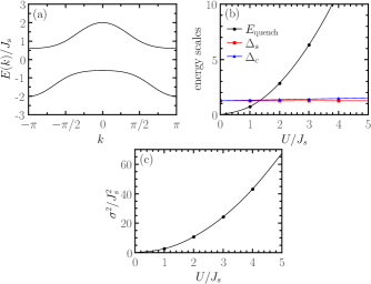
Figure 1: (a) The noninteracting ($\hat{\mathcal{H}}_{U}\equiv 0$) band structure, $E(k)$, of the Hamiltonian defined in Eq. (1). (b) The energy of the quench and the charge and spin gaps (in units of $J_{s}$) as a function of the Hubbard interaction for $L=80$. (c) The variance (Eq. (9)) of the initial state with respect to the quench Hamiltonian for $L=80$.

In addition, it can also be classified as a $Z_{2}$ band insulator due to the special form of the hybridization term.Zhong et al. (2017) If the hopping amplitudes had opposite signs, the ground state would be metallic and the topological reasoning would not make sense. The ground-state properties of the model have been studied recently, and it turned out that the noninteracting ground state is adiabatically connected to the interacting one,Lisandrini et al. (2017) that is, no topological phase transition takes place as $U$ is switched on. In the present work we address the scenario that the system is prepared in the initially noninteracting ground state:

$$\hat{\mathcal{H}}(U_{i}=0)|\Psi_{0}\rangle=E_{0}|\Psi_{0}\rangle$$ (5)

assuming that the ground state has no net magnetic moments, and then we evolve it with the interacting Hamiltonian:

$$|\Psi(t)\rangle=e^{-i\hat{\mathcal{H}}(U_{f}=U)t}|\Psi_{0}\rangle.$$ (6)

In what follows $\langle\dots\rangle(t)$ denotes expectation value over $|\Psi(t)\rangle$.

The time evolution is performed using the TDVP method,Haegeman et al. (2011, 2016) which does not require a manual partition of the Hamiltonian into non-overlapping parts and we can avoid the Trotter-Suzuki decomposition of the time-evolution operator and the use of swap gates. On the other hand it introduces a projection error but this is much smaller than the truncation error (which is controlled during the simulation), since the time evolution is started from a fairly entangled state. In our simulations the total discarded weight was set to $10^{-7}$, and the largest bond dimension used was $\sim 6000$. We considered chains with lengths $L=40-80$ and show results for system size $L=80$ (unless stated otherwise) for which the finite-size effects were negligible. We compared runs with different total discarded weights and show only data that are indistinguishable on the scale of the figures. The ground-state calculations were performed using the standard DMRG procedure,White (1992, 1993); Schollwöck (2005); Hallberg (2006); Hubig et al. (2015) while finite-temperature calculations were obtained with the ancilla method.Verstraete et al. (2004)

III Results

Before diving into the details of the quench dynamics, it is instructive to look at how the low-energy charge and spin excitations relate to the energy of the quench. Since we consider chains with open boundary conditions, we must adopt a different definition of the spin and charge gap to rule out the gapless edge modes in the system:

$$\begin{split}\Delta_{s}(L)&=E_{0}(2,2L)-E_{0}(0,2L),\\ \Delta_{c}(L)&=E_{0}(0,2L+4)-E_{0}(0,2L),\end{split}$$ (7)

where $E_{0}(T^{z},N)$ is the ground-state energy with total magnetization $T^{z}$ and number of electrons, $N$. The definition for the spin gap is analogous to the definition of the Haldane gap in spin systems. Similar considerations apply for the charge gap, namely, at half filling the edge modes already host two fermions and can host up to four fermions altogether, thus, we need to add four fermions to the system to obtain a bulk excitation, while keeping the total magnetization zero. The energy of the quench by definition is:

$$E_{\mathrm{quench}}(U)=\langle\Psi_{0}|\hat{\mathcal{H}}(U)|\Psi_{0}\rangle-\langle\Psi_{U}|\hat{\mathcal{H}}(U)|\Psi_{U}\rangle,$$ (8)

where $|\Psi_{U}\rangle$ denotes the ground state of $\hat{\mathcal{H}}(U)$. These quantities are plotted together in Fig. 1(b). For weak quenches, $U\lesssim 2$, the quench does not really probe the higher lying excitations; however, above this value the energy of the quench becomes much larger than the first excitations in the spin and charge sectors that are roughly constant as $U$ is increased. Besides the quench energy, it is also instructive to calculate the variance, $\sigma^{2}$ of the initial state with respect to the quench Hamiltonian:

$$\sigma^{2}(U)=\langle\Psi_{0}|\hat{\mathcal{H}}^{2}(U)|\Psi_{0}\rangle-\langle\Psi_{0}|\hat{\mathcal{H}}(U)|\Psi_{0}\rangle^{2}.$$ (9)

This enables us to estimate what fraction of excitations takes part in the quench. The variance is shown in Fig. 1(c) and increases as $\sigma^{2}\propto U^{2}$. Based on these observation, we may expect qualitatively different behavior for $U\lesssim 2$ and $U\gtrsim 2$.

III.1 Local observables

First, we investigate the time evolution of the double occupancy on the $s$-wave chain:

$$d^{s}(t)=\frac{1}{L}\sum_{j=1}^{L}\left\langle\hat{n}^{s}_{j\uparrow}\hat{n}^{s}_{j\downarrow}\right\rangle(t),$$ (10)

since this quantity is readily accessible in quantum gas experiments.Ronzheimer et al. (2013); Strohmaier et al. (2010) The time evolution of $d^{s}$ is shown in Figs. 2 (a)-(c) following the interaction quenches from $U_{i}=0$ to $U_{f}=U$.

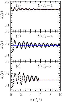
Figure 2: Time evolution of double occupancy on the $s$-wave chain after the interaction quench from $U_{i}=0$ to $U_{f}=U$ as indicated in the figures. In case of $U/J_{s}=6$ we were not able to go beyond $t\approx 6J_{s}^{-1}$ due to entanglement growth. The dashed lines denote the corresponding thermal averages.

Since the system is initially prepared in an uncorrelated state, the double occupancy at $t=0$ is very close to $1/4$ although the hybridization between the two orbitals is present. We observe that the data can be fitted reasonably well with the function

$$d^{s}(t)=a\sin(\omega t+\phi)\exp(-t/\tau)+\bar{d}^{s}.$$ (11)

For strong quenches ($U/J_{s}\gtrsim 3$) we discarded the transient behavior for $t\lesssim 2$ in the fitting procedure. To characterize the postquench dynamics it is worth investigating how the fitting parameters depend on the model parameters. We could reach long enough times up to $U/J_{s}=5$ to reliably use the fitting function. The results are shown in Fig. 3.

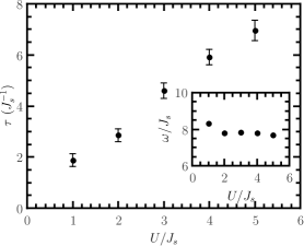
Figure 3: The main and inset figures show the relaxation time, $\tau$, and the frequency of the oscillation, $\omega$, respectively, as a function of the Hubbard interaction. The error bars are the asymptotic standard error resulting from the least-squares fit of Eq. (11) to the data.

We observe that the relaxation time increases linearly with the Hubbard interaction strength, which is perfectly consistent with the a priori expectations concluded from Fig. 1, since for large interaction strength the quench drives the system far away from the equilibrium ground state and the slower the system relaxes the larger the Hubbard interaction strength is. On the other, the frequency of the oscillation do not exhibit any significant dependence on the interaction strength, it remains roughly constant, $\omega\approx 8J_{s}$.

One can also extract the time average of the double occupancy, $\bar{d}^{s}$ from the fit results or by averaging the above data for $t\gtrsim 2/J_{s}$. The latter one is used for calculating the time-averaged quantities later on. To address the question of thermalization, we compare them with the corresponding thermal averages in Fig. 4.

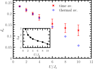
Figure 4: Time and thermal average of the double occupancy on the $s$-wave chain as a function of the postquench interaction value. The error bars show the standard deviation from the mean value. The inset figure shows the effective inverse temperature as a function of the postquench interaction value.

The thermal ensemble is defined by the density matrix $\hat{\rho}(\beta)=e^{-\beta_{\rm eff}\hat{\mathcal{H}}}/\mathcal{Z}$, where $\mathcal{Z}$ is the partition function and the effective inverse temperature, $\beta_{\rm eff}$, is determined from the following relation:

$$\langle\Psi_{0}|\hat{\mathcal{H}}(U_{f}=U)|\Psi_{0}\rangle={\rm Tr}\left[\hat{\mathcal{H}}(U_{f}=U)\hat{\rho}(\beta)\right].$$ (12)

It is readily seen that the postquench time averages are in a very good agreement with the thermal averages corresponding to the postquench $U$ as long as $U$ is relatively weak. These results suggest that the double occupancy thermalizes for $U/J_{s}\lesssim 6$, however, for $U/J_{s}\gtrsim 6$ a discrepancy is observed indicating a nonthermal value. A possible explanation can be that the thermalization time is much longer than the time reachable in our simulation, and the time averages in our time window are different from those in the steady state. The inverse effective temperature satisfying Eq. (12) as a function of the postquench $U$ is shown in the inset of Fig. 4, where the expected divergence for $U\rightarrow 0$ is visible.

It is also instructive to study the local spin correlations between the $s$ and $p$ electrons, which is shown in Fig. 5 together with the corresponding thermal averages.

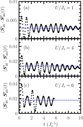
Figure 5: Time evolution of local spin correlation between the $s$ and $p$ electrons measured in the middle of the $L=80$ chain, after the interaction quench from $U_{i}=0$ to $U_{f}=U$ as indicated in the figures. The dashed lines denote the corresponding thermal averages.

The spin operators for fermion species $a\in\{s,p\}$ are defined as

$$\hat{\boldsymbol{S}}_{j}^{a}=\frac{1}{2}\sum_{\beta\gamma}\hat{a}^{\dagger}_{j\beta}\boldsymbol{\sigma}^{\phantom{\dagger}}_{\beta\gamma}\hat{a}^{\phantom{\dagger}}_{j\gamma},$$ (13)

where $\boldsymbol{\sigma}$ is the vector of Pauli matrices. Initially the correlation between the two types of electrons is zero due to the uncorrelated state, then ferromagnetic correlation develops similarly to the equilibrium case in the presence of interaction. The emergence of local ferromagnetic correlations can be understood from the following argument. Switching on the interaction results in antiferromagnetic nearest-neighbor correlations among the $s$ electrons, that is, $\langle\hat{\boldsymbol{S}}_{j}^{s}\hat{\boldsymbol{S}}_{j+1}^{s}\rangle<0$. The correlation between nearest-neighbor $s$ and $p$ electrons are also antiferromagnetic, $\langle\hat{\boldsymbol{S}}_{j}^{s}\hat{\boldsymbol{S}}_{j+1}^{p}\rangle<0$, since the hybridization term, which connects these sites, favors the formation of a singlet. (In the conventional Anderson lattice, this hybridization is on-site and prefers to have a local Kondo singlet.) We can repeat the same argument for sites $(j-1,j)$, from which one can quickly see that the correlation $\langle\hat{\boldsymbol{S}}_{j}^{s}\hat{\boldsymbol{S}}_{j}^{p}\rangle$ should be ferromagnetic. Thus the two $S=1/2$ fermions in the lattice form a $S=1$ object in each site, which are coupled antiferromagnetically. This is also the reason why the present system resembles to the Haldane phase. Regarding the thermalization, it also exhibits similarities to the double occupancy; for $U/J_{s}\lesssim 3$ the time-averages agree well with those of the thermal ensemble. The discrepancy at larger values of $U$ can be explained by the previous argument for the thermalization time.

III.2 Nonlocal observables and edge states

In what follows we focus on the behaviour of nonlocal quantities following the interaction quench. Previously it was shown, that the noninteracting ground state is adiabatically connected to the interacting caseLisandrini et al. (2017) (both being in the Haldane phase); however, it is not trivial what happens to its topological properties when the interaction is abruptly turned on. The Haldane phase is generically characterized by the breaking of a hidden $Z_{2}\times Z_{2}$ symmetry, which implies a symmetry-protected topological order manifesting itself in (i) an evenly degenerate entanglement spectrum, (ii) 3 nonvanishing string order parameters and (iii) a ground-state degeneracy depending on the boundary conditions.Pollmann et al. (2010); Turner et al. (2011); Pollmann and Turner (2012) In this subsection we address the time-dependent properties of the entanglement spectrum, string order parameter and the edge states. The entanglement spectrum, $\Lambda_{j}$, is immediately accessed by performing a Schmidt decomposition of the wave function into two halves:

$$\left|\Psi\right\rangle=\sum_{j}\Lambda_{j}|\phi_{j}\rangle_{A}|\phi^{\prime}_{j}\rangle_{B}.$$ (14)

The presence of the diluted antiferromagnetic order is characterized by the string operator:

$$\hat{\mathcal{O}}^{\alpha}_{\ell}=\hat{T}_{j}^{\alpha}\left[\prod_{n=j+1}^{j+\ell-1}e^{i\pi\hat{T}_{n}^{\alpha}}\right]\hat{T}_{j+\ell}^{\alpha}\quad(\alpha\in\{x,y,z\}).$$ (15)

The ground state of a system exhibits string order when the string order parameter, $\mathcal{O}^{\alpha}$ fulfills

$$\mathcal{O}^{\alpha}=\lim_{\ell\rightarrow\infty}\left\langle\hat{\mathcal{O}}^{\alpha}_{\ell}\right\rangle\neq 0$$ (16)

for any $\alpha$, or alternatively in the time-dependent case:

$$\mathcal{O}^{\alpha}(t)=\lim_{\ell\rightarrow\infty}\left\langle\hat{\mathcal{O}}^{\alpha}_{\ell}\right\rangle(t)\neq 0.$$ (17)

In Eq. (15) $\hat{T}_{j}^{\alpha}$ is the appropriate component of the total spin operator at site $j$:

$$\hat{\boldsymbol{T}}_{j}=\hat{\boldsymbol{S}}_{j}^{s}+\hat{\boldsymbol{S}}_{j}^{p}.$$ (18)

Due to the $\mathrm{SU}(2)$ symmetry of the Hamiltonian (1), it is sufficient to consider one of the three string order operators, therefore we concentrate on $\hat{\mathcal{O}}^{z}_{\ell}$ in the following.

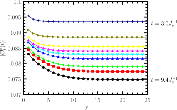
Figure 6: String correlations after the interaction quench from $U_{i}=0$ to $U_{f}/J_{s}=4$ as a function of length $\ell$. Each line corresponds to a different time ranging from $t=3J_{s}^{-1}$ (top) to $t=9.4J_{s}^{-1}$ (bottom) with time spacing $0.8J_{s}^{-1}$.

We first discuss the behavior of the string operator for various lengths and times ($t>3J_{s}^{-1}$ to exclude the transient behavior at short times), which is shown in Fig. 6. It is observed that the string correlations start decreasing after the quench. It is also immediately seen that $\mathcal{O}^{z}(t)$ is approached exponentially as the string length is increased, furthermore, the more time has elapsed the slower the expectation value of the string operator reaches its thermodynamic value, which is demonstrated by Fig. 7.

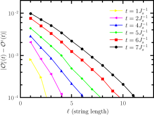
Figure 7: Deviation of string correlations from their thermodynamic value as a function of string length measured at different times on a log-lin scale for $U_{f}/J_{s}=5$.

Next we turn our attention to the string order parameter, shown in Fig. 8 after different interaction quenches.

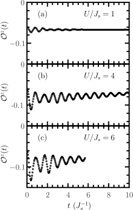
Figure 8: Time evolution of string order parameter following the interaction quench from $U_{i}=0$ to $U_{f}=U$ as indicated in the figures.

In agreement with the previous finding,Lisandrini et al. (2017) the system exhibits string order even for $U=0$. The string order parameter remains nonzero after the quench as well but its absolute value starts decreasing, which might vanish in the steady state at $t\rightarrow+\infty$, but longer times are out of reach due to entanglement growth. This feature is more emphasized for stronger quenches, that is, $U/J_{s}\gtrsim 4$. For weak interaction quenches this behavior is not observed, which may originate from the fact that the defect density is low, thus, the thermalization time may be very long and the decay is not visible at this time scale.

It is important to note; however, that the string order parameter is a basis-dependent quantity, and its decrease or alleged disappearance is not sufficient evidence for the destruction of the topological properties. Therefore it is also intriguing to analyze the entanglement spectrum after the quench, which is another hallmark of symmetry-protected topological phases and basis-independent. For better visibility we consider only the largest 4 Schmidt values, which are plotted in Fig. 9, but the higher lying values also exhibit qualitatively similar behavior.

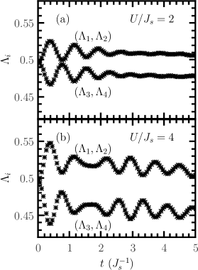
Figure 9: Time evolution of the low-lying entanglement spectrum after the interaction quench from $U_{i}=0$ to $U_{f}=U$. The consecutive Schmidt values are denoted by $\times$ and $+$, respectively.

It is immediately observed that the initially fourfold degenerate Schmidt value becomes twofold degenerate following the interaction quench. As we would expect from the nonzero string order parameter, the degeneracy of the spectrum is also preserved for finite times. The crossover of the fourfold degeneracy into two twofold degenerate branches after the quench is analogous to what happens when one consider the evolution of the entanglement spectrum of the ground state as a function of $U$.

Based on the splitting in the entanglement spectrum at $U=0$, one may think that the edge states of the steady state should exhibit similar behavior as the ground state does for finite $U$. Namely, the ground state for $U=0$ and $\sum_{j}T_{j}^{z}=0$ has a holon and a doublon edge state resulting in a vanishing spin profile, but a nonuniform charge profile at the edges.Lisandrini et al. (2017) For $U>0$ these edge states become excited states, while the spin-1/2 edge states possess lower energy hence it results in a uniform charge distribution and an accumulation of 1/2 spins at the edges, forming a singlet. To see what happens in the quenched states, we investigated the difference in the spatial charge profile, $\Delta n_{j}$ (Fig. 10), defined as:

$$\Delta n_{j}(t)=\left\langle n_{j}\right\rangle(t)-n_{0},$$ (19)

where $n_{j}=n_{j}^{s}+n_{j}^{p}$ is the total particle number operator at site $j$ and $n_{0}=2$ is the average occupancy per site in the half-filled case.

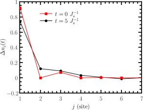
Figure 10: Charge profile at the left edge of the system in the initial state and after a quench with $U_{f}/J_{s}=4$.

Surprisingly, the charge edge states appear to be frozen during the interaction quench and the spin profile remains identically zero (not shown) despite the fact that there is a finite $U$ present in the system. This fact clearly indicates that the quenched system will preserve the topological order at finite times but its properties are different from what one would naively expect.

Due to the fact that the time-evolved state exhibits similar topological properties as the initial state, it is interesting to consider the Loschmidt echo during the time evolution:

$$\mathcal{L}(t)=|\langle\Psi_{0}|\Psi(t)\rangle|^{2},$$ (20)

which precisely quantifies the deviation of the time-evolved state from initial one. This is shown in Fig. 11(a) for several values of the Hubbard interaction strength.

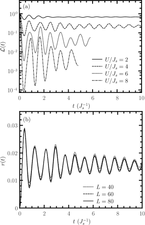
Figure 11: (a) Loschmidt echo (using a log-lin scale) after the quench with different values of $U$, and $L=40$. (b) The rate function for $U/J_{s}=4$ and different system sizes.

It is observed that for weak interaction quenches ($U/J_{s}\lesssim 2$), the Loschmidt echo is fairly large $\mathcal{L}(t)\sim 0.7$. This may not surprise us if we recall Fig. 1(b), that is, the quench energy is comparable with the energy of the low-lying excitations, meaning that the system remains close the initial state. What is more remarkable is that the Loschmidt echo saturates to a value of $\mathcal{L}(t)\sim 0.2$ even for $U/J_{s}=4$, when the quench pushes the system far away from the ground state, and similarly, it also oscillates around a finite value for other Hubbard interaction strengths. Since the Loschmidt echo, in general, is expected to decay exponentially in time in ergodic systems, we conclude that the quench does not drive the system to completely explore the Hilbert space, but it remains trapped in a region close to the initial state, in spite of the fact that the quench energy is quite large compared to the gaps in the system. One can naturally ask if the above statements based on the Loschmidt echo hold in the thermodynamic limit. Since the Loschmidt echo itself is not applicable for infinite system size, one usually introduces the rate function, $r(t)$:

$$r(t)=-\frac{1}{L}\log[\mathcal{L}(t)],$$ (21)

which has a well-defined thermodynamic limit. We calculated this quantity for different chain lengths in Fig. 11(b) to address the finite-size effects. We can observe that $r(t)$ exhibits a weak size-dependence (in agreement with the short correlation length from Fig. 7), which supports our arguments based on the Loschmidt echo.

IV Conclusions

We have presented a numerical analysis of an interaction quench in a 1D topological Kondo insulator modelled by a $p$-wave Anderson lattice model with nonlocal hybridization. We studied the time evolution and thermalization of different observables: double occupancy and local spin correlations. In addition we addressed the behavior of several other quantities, including the string order parameter and entanglement spectrum directly related to the topological properties. In case of double occupancy and local spin correlations we found that the thermalization already occurs in our simulation up to interaction strength $U/J_{s}\sim 6$ and $U/J_{s}\sim 3$, respectively, while for stronger quenches the thermalization time is expected to be much longer, which accounts for the difference between the time and thermal averages.

Then we turned our attention to the topological properties of the system. We pointed out that the topological order is preserved in the time-evolved state. Although the decreasing value of the string order parameter at first glance would indicate that the steady state might possesses a trivial topology, this can be ruled out by examining the entanglement spectrum and Loschmidt echo, which are basis independent quantities unlike the string order parameter. We demonstrated that the entanglement spectrum preserves its doubly degenerate property and the initial charge edge states remain frozen during the time evolution instead of the appearance of magnetic edge states. Moreover, the Loschmidt echo tends to a finite value during the time evolution, clearly indicating that the time-evolved state remains in the same phase.

Our results could be directly tested in cold atom experiments, since the charge profile or double occupancies can be routinely measured,Ronzheimer et al. (2013); Strohmaier et al. (2010); Cheuk et al. (2016); Parsons et al. (2016); Cocchi et al. (2016) moreover, the string correlations have also been extracted in cutting-edge experiments.Hilker et al. (2017) Since the interaction can be varied using Feshbach resonances, the presented quench scheme could also be experimentally realized.