Algebraic Localization from Power-Law Interactions in Disordered Quantum Wires

Abstract

We analyze the effects of disorder on the correlation functions of one-dimensional quantum models of fermions and spins with long-range interactions that decay with distance $\ell$ as a power-law $1/\ell^{\alpha}$. Using a combination of analytical and numerical results, we demonstrate that power-law interactions imply a long-distance algebraic decay of correlations within disordered-localized phases, for all exponents $\alpha$. The exponent of algebraic decay depends only on $\alpha$, and not, e.g., on the strength of disorder. We find a similar algebraic localization for wave-functions. These results are in contrast to expectations from short-range models and are of direct relevance for a variety of quantum mechanical systems in atomic, molecular and solid-state physics.

Quantum waves are generally localized exponentially by disorder. Following the seminal work by Anderson with spin-polarized electrons Anderson (1958) much experimental Roati et al. (2008); Billy et al. (2008); Kondov et al. (2011); Jendrzejewski et al. (2012); Schreiber et al. (2015); Smith et al. (2016); Bordia et al. (2016) and theoretical interest has been devoted to the study of localized phases and to the localization-delocalization transition for non-interacting and interacting quantum models Lee and Ramakrishnan (1985); Altshuler et al. (1997); Basko et al. (2006); Oganesyan and Huse (2007); Gornyi et al. (2005); Žnidarič et al. (2008); Biddle et al. (2009); Biddle and Das Sarma (2010); Biddle et al. (2011); Pal and Huse (2010); Luca and Scardicchio (2013); Vosk and Altman (2013); Bar Lev and Reichman (2014); Bar Lev et al. (2015); Luitz et al. (2015); Luitz (2016); Naldesi et al. (2016); Nandkishore et al. (2014); Gornyi et al. (2017); Potter and Vasseur (2016).

While most works have focused on short-range couplings, long-range hopping and interactions that decay with distance $\ell$ as a power-law $1/\ell^{\alpha}$ have recently attracted significant interest Kastner (2010); Gong et al. (2014); Foss-Feig et al. (2015); Hauke and Tagliacozzo (2013); Eisert et al. (2013); Schachenmayer et al. (2013); Métivier et al. (2014); Kastner and van den Worm (2015); Cevolani et al. (2015, 2016); Bettles et al. (2017); Frérot et al. (2017, 2018) as they can be now engineered in a variety of atomic, molecular and optical systems. For example, power-law spin interactions with tunable exponent $0<\alpha<3$ can be realized in arrays of laser-driven cold ions Schneider et al. (2012); Richerme et al. (2014); Jurcevic et al. (2014); Britton et al. (2012); Bermudez et al. (2013) or between atoms trapped in a photonic crystal waveguide Shahmoon and Kurizki (2013); Douglas et al. (2015); Litinskaya et al. (2016); Vaidya et al. (2018); dipolar-type $1/\ell^{3}$ or van-der-Waals-type $1/\ell^{6}$ couplings have been experimentally demonstrated with ground-state neutral atoms Kadau et al. (2016); Lepoutre et al. (2018); Baier et al. (2018); Tang et al. (2018), Rydberg atoms Weimer et al. (2008); Saffman et al. (2010); Viteau et al. (2012); Schauß et al. (2012); Carr et al. (2013); Barredo et al. (2014); Balewski et al. (2014); Jau et al. (2015); Weber et al. (2015); Faoro et al. (2016); Labuhn et al. (2016); Gorniaczyk et al. (2016); Zeiher et al. (2016); Bernien et al. (2017); Piñeiro Orioli et al. (2018), polar molecules Yan et al. (2013); Hazzard et al. (2014); Reichsöllner et al. (2017) and nuclear spins Álvarez et al. (2015). In solid state materials, power-law hopping is of interest for, e.g., excitonic materials Anderson et al. (1998, 2002); Scholes and Rumbles (2006); Dubin et al. (2005, 2006); Vögele et al. (2009); Wüster et al. (2011); Günter et al. (2013); Robicheaux and Gill (2014); Schönleber et al. (2015); Schempp et al. (2015); Barredo et al. (2015); Rosenberg et al. (2018), while long-range $1/\ell$ coupling is found in helical Shiba chains Pientka et al. (2013, 2014), made of magnetic impurities on an s-wave superconductor. In many of these systems, disorder - in particles’ positions, local energies, or coupling strengths - is an intrinsic feature, and understanding its effects on single-particle and many-body localization remains a fundamental open question.

For non-interacting models, it is generally expected that long-range hopping induces delocalization in the presence of disorder for $\alpha<d$, while for $\alpha>d$ all wave-functions are exponentially localized Anderson (1958); Rodríguez et al. (2000, 2003); de Moura et al. (2005); Celardo et al. (2016). However, recent theoretical works with positional Deng et al. (2018) and diagonal Celardo et al. (2016) disorder have demonstrated that localization can survive even for $\alpha<d$. Surprisingly, wave-functions were found to be localized only algebraically in these models, in contrast to the usual Anderson-type exponential localization expected from short-range models. How these finding translate to the behavior of wave-functions and, crucially, correlation functions in many-particle systems is not known.

In this work, we investigate the effects of disorder on the decay of correlation functions and wave-functions in long-range quantum wires of fermions and spins. These are extensions of the Kitaev chain with long-range pairing Vodola et al. (2014, 2016); Liu et al. (2018) and the Ising model in transverse field Koffel et al. (2012), corresponding to integrable and non-integable chains in the absence of disorder, respectively. For fermions, we determine the regimes of localization for all $\alpha$ for the cases of disordered hopping or pairing. For the Ising chain, we focus on the regime $\alpha>1$, where the disordered phase diagram has been shown to display many-body localization theoretically Burin (2015) and experimentally Smith et al. (2016). For all models we compute the one-body and two-body connected correlation functions, finding several novel features: (i) The connected correlation functions decay algebraically at long distance within all localized phases, (ii) with an exponent that depends exclusively on $\alpha$, and not, e.g., on the disorder strength. (iii) For the fermionic models, we derive analytic results for the long-distance decay of the correlations that explain the found algebraic decay, in excellent agreement with the numerics. (iv) The same analytical predictions are found to hold also for the correlations of the interacting Ising chain. (v) For any $\alpha$, the localized wave-functions of the fermionic models display a long-distance algebraic decay with exponent $\alpha$, different from recent predictions for long-range hopping models. These results should be of direct relevance to many experiments in cold atomic, molecular and solid-state physics with fermions and spins.

Models.— We consider the following Hamiltonians for one-dimensional long-range fermionic random models

$$H_{{\rm I},{\rm II}}=H_{0}+V_{{\rm I},{\rm II}}$$ (1)

where $H_{0}$ is a homogeneous Hamiltonian given by

$$\begin{split}H_{0}&=-t\sum_{j=1}^{L}\left(a^{\dagger}_{j}a_{j+1}+\mathrm{H.c.}\right)+\mu\sum_{j=1}^{L}n_{j}\\ &+\sum_{j,\ell}\frac{\Delta}{\ell^{\alpha}}\left(a_{j}a_{j+\ell}+\mathrm{H.c.}\right)\end{split}$$ (2)

that describes a $p$-wave superconductor with a long-range pairing, and the indices ${{\rm I},{\rm II}}$ refer to the two different types of Hamiltonians we consider, namely

$$V_{\rm I}=\sum_{j=1}^{L}W_{j}\left(a^{\dagger}_{j}a_{j+1}+\mathrm{H.c.}\right)$$ (3)

that corresponds to a random hopping and

$$V_{\rm II}=\sum_{j,\ell}\frac{W_{j}}{\ell^{\alpha}}\left(a_{j}a_{j+\ell}+\mathrm{H.c.}\right)$$ (4)

that corresponds to a random long-range pairing. In the previous equations, $a^{\dagger}_{j}$ $(a_{j})$ is a fermionic creation (annihilation) operator on site $j$, $\mu$ is the chemical potential, $n_{j}=a^{\dagger}_{j}a_{j}$ and $W_{j}$ are i.i.d random variables drawn from a uniform distribution of width $2W$ and zero mean value. We fix the energy scale by letting $\Delta=2t=1$ and we choose $\mu=2.5$, corresponding to a gapped paramagnetic phase for $W_{j}=0$ Vodola et al. (2014). Different values of $\mu$ do not change the results we find in the following. The random Hamiltonians (1) can be written in diagonal form as $H_{{\rm I},{\rm II}}=\sum_{q=0}^{L-1}\Lambda_{q}\eta^{\dagger}_{q}\eta_{q}$ by a generalized Bogoliubov transformation defined by $\eta_{q}=\sum_{j}(g_{q,j}a_{j}+h_{q,j}a^{\dagger}_{j})$ Lieb et al. (1961), with $\Lambda_{q}$ the energies of the single-particle states labelled by $q$. The ground state $\ket{\Omega}$ is then the vacuum of all quasi-particles $\eta_{q}$ and the matrix elements $g_{q,j}$ and $h_{q,j}$ can be identified with the wave functions of the two fermionic modes $\eta_{q}^{\dagger}$ and $\eta_{q}$, respectively.

As an interacting model, we consider the following random long-range Ising model Koffel et al. (2012) in transverse field

$$H_{\text{LRI}}=\sum_{j,\ell}{(\sin\theta+B_{j})}\frac{\sigma^{x}_{j}\sigma^{x}_{j+\ell}}{\ell^{\alpha}}+\sum_{j=1}^{L}(\cos\theta+W_{j})\sigma^{z}_{j},$$ (5)

where $\sigma_{j}^{\nu}$ ($\nu=x,z$) are Pauli matrices for a spin-1/2 at site $j$ and $B_{j}$ are i.i.d random variables drawn from a uniform distribution of width $2B$ and zero mean value. We choose $\theta=\pi/5$, corresponding to a paramagnetic phase for $B_{j}=W_{j}=0$ Vodola et al. (2016). Different values of $\theta$ will not change the results we find in the following. For any finite disorder strength, the model Eq. (5) has been shown to display a many-body localized (MBL) phase for $\alpha>2$ Hauke and Heyl (2015); Li et al. (2016); Maksymov et al. (2017).

In the following, we first determine the regimes of localization for the fermionic models Eqs. (1) and then compute the single- and two-body correlation functions, as well as the wave-functions, within the localized phases using a combination of analytical and numerical techniques. For the long-range Ising model Eq. (5) we compute the spin-spin connected correlation functions numerically. Our goal is to demonstrate that all these quantities decay algebraically at large distances both for non-interacting and interacting MBL localized models and to characterize their decay exponents.

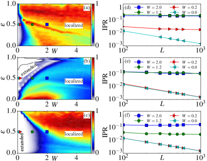
Figure 1: Left panels: IPR in the thermodynamic limit as a function of the disorder strength $W$ and the rescaled energy $\epsilon$ for (a) $\alpha=3$ and (b) $\alpha=0.8$ for the model (I) with random hopping and (c) for $\alpha=3.0$ for the model (II) with random pairing. In panel (b) the solid black line marks the region where the number of extended states is too low for a meaningful data analysis. Only in these panels, for drawing purpose, the IPR has been rescaled to 1 in correspondence of its maximum value. Right panels: Scaling of the IPR as a function of the system size $L$ for $\epsilon=1/2$ and different $W$ for (d) $\alpha=3$ and (e) $\alpha=0.8$ for the model (I) and (f) for $\alpha=3.0$ for the model (II). In panels (a-c) the symbols indicate the values of $W$ and $\epsilon$ we choose to plot the IPR in panels (d-f).

Localized phases of disordered fermions.— We determine the localized phases for Hamiltonians Eqs. (1) by combining information from the numerical calculation of the inverse participation ratio (IPR) and the entanglement entropy sup . The IPR gives information about the spatial extension of single-particle states and is defined as $\mathrm{IPR}_{q}={\sum_{j=1}^{L}[{\lvert g_{q,j}\rvert^{4}+\lvert h_{q,j}\rvert^{4}}]}$ for a normalized state with energy $\Lambda_{q}$. The IPR tends to zero for increasing $L$ for extended states, while it remains finite for localized states. If a value for the energies $\Lambda_{q}$ exists that separates extended states from localized states the system is said to display a (single-particle) mobility edge.

For comparing the IPR of states with different energies, we rescale the $\Lambda_{q}$ (obtained for $\sim 200$ disorder realizations) according to $\epsilon_{q}=(\Lambda_{q}-\Lambda_{\text{min}})/(\Lambda_{\text{max}}-\Lambda_{\text{min}})$, with $\Lambda_{\text{max}}$ ($\Lambda_{\text{min}}$) the maximum (minimum) value of the energies $\Lambda_{q}$. We then bin the different levels into groups with equal energy width, we average the IPR within each bin. Finally, in order to obtain the phase diagrams, we perform a finite-size scaling of the obtained IPR in the limit $L\to\infty$ sup .

Figure 1 shows exemplary results for IPR as a function of $W$ and $\epsilon$ for model Eqs. (1) (I) [for $\alpha=3$ and 0.8 in panels (a) and (b), respectively], and (II) [for $\alpha=3$ in panel (c)] together with examples of finite size scaling [panels (d-e)]. The figure shows that the phase diagrams are much richer than expected from pure long-range hopping models: For model (I) with disordered hopping and $\alpha>1$ [panel (a)] essentially all states are localized. For $\alpha<1$ [panel (b)] we find that, at $W$ fixed, there exists a mobility edge below (above) which all the states are localized (delocalized). For model (II) [panel (c)] with disordered pairing when $\alpha>1$ localized states are present at all energies if $W\gtrsim 2$, while we find a mobility edge for $\alpha>1$ and $W\lesssim 2$: all states are delocalized at low energy $\epsilon$ and localized for higher $\epsilon$. Below we focus on the identified localized phases and compute the correlation functions and wave-functions for all models.

Correlation functions.— We consider the single-particle correlator $C(j,\ell)=\braket{a^{\dagger}_{j}a_{j+\ell}}_{W}$ for the two free-fermionic models of Eqs. (1) as well as the spin-spin correlation function $S_{\nu}(j,\ell)=\left[\braket{\sigma^{\nu}_{j}\sigma^{\nu}_{j+\ell}}-\braket{\sigma^{\nu}_{j}}\braket{\sigma^{\nu}_{j+\ell}}\right]_{W}$ (for $\nu=x,z$) for the interacting long-range Ising model of Eq. (5). In the definitions of $C(j,\ell)$ and $S_{\nu}(j,\ell)$ the subscript $W$ indicates averaging over the disorder distribution. For models with short-range interactions, all the correlation functions decay exponentially with $\ell$. Here we are interested in the effects of long-range interactions.

Figures 2(a) and (b) show representative results for the correlator $C(\ell):=C(j_{0},\ell)$ for models $H_{\text{I}}$ and $H_{\text{II}}$, respectively, for different values of $\alpha$. We choose $j_{0}=L/4$ far from the edges in order to avoid boundary effects. We find numerically that the long-distance decay of $C(\ell)$ is always of power-law type $C(\ell)\sim\ell^{-\gamma}$ for all $\alpha$ within localized phases. In particular, for model $H_{\text{I}}$ [panel (a)] and $\alpha<1$ the decay is essentially algebraic at all distances with $\gamma\sim{2-\alpha}$, while for $\alpha>1$ we find for both models a hybrid decay that is exponential at short distances and power-law at large distances, with $\gamma\sim{\alpha}$ [panels (a) and (b)]. Remarkably, we find that the values of the decay exponents of the power-law tails do not depend on the disorder strength $W$ sup .

This surprising long-distance behavior of correlations can be understood by computing the correlations analytically treating disorder as a perturbation. Here, we focus on model (I) with perturbation $V_{\rm I}$, while a similar argument can be applied also to (II). The homogeneous Hamiltonian $H_{0}$ can be diagonalised via Fourier and Bogoliubov transformations as $H_{0}=\sum_{k}\lambda_{\alpha}(k)\xi^{\dagger}_{k}\xi_{k}$, where $\lambda_{\alpha}(k)=[\left(\cos k-\mu\right)^{2}+4f_{\alpha}^{2}(k)]^{1/2}$ and $\xi_{k}$ are extended Bogolioubov quasi-particles related to the unperturbed fermionic operators in momentum space via $\tilde{a}_{k}=v_{k}\xi_{k}-u_{k}\xi^{\dagger}_{-k}$ with $v_{k}=\cos\varphi(k)$ and $u_{k}=\mathrm{i}\sin\varphi(k)$, with $\tan 2\varphi(k)=f_{\alpha}(k)/[\mu-\cos k]$ and $f_{\alpha}(k)=\sum_{\ell=1}^{L-1}\sin(k\ell)/\ell^{\alpha}$ . At first order in $W_{j}$ the ground state $\ket{\Omega_{0}}$ of the unperturbed Hamiltonian $H_{0}$ is modified by $V_{\rm I}$ as

$$\ket{\Omega}=\ket{\Omega_{0}}+\ket{\delta\Omega_{0}}=\ket{\Omega_{0}}-\sum_{kk^{\prime}}{J}_{k,k^{\prime}}A(k,k^{\prime})\xi^{\dagger}_{k}\xi^{\dagger}_{k^{\prime}}\ket{\Omega_{0}},$$ (6)

where we define $J_{k,k^{\prime}}=-\sum_{j}e^{\mathrm{i}(k-k^{\prime})j}W_{j}/L$ and $A(k,k^{\prime})=2(\text{e}^{\mathrm{i}k}+\text{e}^{-\mathrm{i}k^{\prime}})v_{k}u^{*}_{k^{\prime}}/[\lambda(k)+\lambda(k^{\prime})]$. Since $\braket{J_{k,k^{\prime}}}_{W}=0$, we note that the terms $\braket{\delta\Omega_{0}}{a^{\dagger}_{j}a_{j+\ell}}{\Omega_{0}}_{W}$ and $\braket{\Omega_{0}}{a^{\dagger}_{j}a_{j+\ell}}{\delta\Omega_{0}}_{W}$ vanish due to averaging over the disorder distribution. Thus, we obtain the following expression for $C(\ell)$

$$\braket{\Omega}{a^{\dagger}_{j}a_{j+\ell}}{\Omega}_{W}=\braket{\Omega_{0}}{a^{\dagger}_{j}a_{j+\ell}}{\Omega_{0}}+\braket{\delta\Omega_{0}}{a^{\dagger}_{j}a_{j+\ell}}{\delta\Omega_{0}}_{W}.$$ (7)

The first term in the r.h.s. of Eq. (7) corresponds to the correlator of the homogeneous system Vodola et al. (2016) that is $\braket{\Omega_{0}}{a^{\dagger}_{j}a_{j+\ell}}{\Omega_{0}}=\int_{0}^{2\pi}\mathrm{d}k\ \text{e}^{\mathrm{i}k\ell}R_{0}(k)$, with $R_{0}(k)=\lvert u_{k}\rvert^{2}$. The second term arises instead because of the random part of the Hamiltonian and reads

$$\braket{\delta\Omega_{0}}{a^{\dagger}_{j}a_{j+\ell}}{\delta\Omega_{0}}_{W}=\frac{2W^{2}}{3}\int_{0}^{2\pi}\mathrm{d}k\ \text{e}^{\mathrm{i}k\ell}R_{1}(k),$$ (8)

where we have defined $R_{1}(k)=[c-{U}(k)]\lvert u_{k}\rvert^{2}-{V}(k)\lvert v_{k}\rvert^{2}$, with $c$ that does not depend on $k$ sup , $V(k)=\sum_{p}A(p,k)A(k,p)\sim f_{\alpha}(k)/\lambda_{\alpha}(k)$ and $U(k)=V(-k)$. The behaviour of both integrals for $\ell\to\infty$ can be extracted by integrating $R_{0}(k)$ and $R_{1}(k)$ for $k\to 0$. In this limit, $f_{\alpha}(k)$, and thus the single-particle energy $\lambda_{\alpha}(k)$, display a non-analytical scaling $f_{\alpha}(k)\sim\lvert k\rvert^{\alpha-1}$ sup . For the first term in the r.h.s. of Eq. (7) the latter behavior results in (details in Ref. sup )

$$\braket{\Omega_{0}}{a^{\dagger}_{j}a_{j+\ell}}{\Omega_{0}}\sim\begin{cases}{1}/{\ell^{2-\alpha}}&\text{for }\alpha<1\\ {1}/{\ell^{2\alpha-1}}&\text{for }1<\alpha<2\\ {1}/{\ell^{\alpha+1}}&\text{for }\alpha>2\end{cases}$$ (9)

which corresponds to the expected long-distance power-law decay of correlation functions for the homogeneous gapped superconductor with long-range pairing Vodola et al. (2014, 2016); Lepori et al. (2016); Maghrebi et al. (2016); Lepori et al. (2017). Instead, for $R_{1}(k)$ the scaling of $f_{\alpha}(k)$ near $k\to 0$ implies

$$R_{1}(k)\sim\begin{cases}k^{1-\alpha}&\text{for }\alpha<1\\ k^{\alpha-1}&\text{for }\alpha>1\end{cases}$$ (10)

which entails the following form of the disordered part of $C(\ell)$

$$\braket{\delta\Omega_{0}}{a^{\dagger}_{j}a_{j+\ell}}{\delta\Omega_{0}}_{W}\sim\begin{cases}{W^{2}}/{\ell^{2-\alpha}}&\text{for }\alpha<1\\ {W^{2}}/{\ell^{\alpha}}&\text{for }\alpha>1\end{cases}$$ (11)

after the integration of $R_{1}(k)$ in Eq. (8) sup .

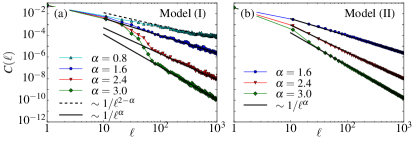
Figure 2: (a) Correlation function $C(\ell)$ for the model (I) as a function of the lattice site $\ell$ for different values of $\alpha$ and for $W=5$, $L=2000$ and 400 disorder realizations. The power-law tails are fit by the black lines scaling as $1/\ell^{2-\alpha}$ (dashed) and $1/\ell^{\alpha}$ (solid) in agreement with the analytical results in Eq. (11). (b) Same as panel (a) but for the model (II).

The discussion above demonstrates the following surprising results: (i) For $\alpha<1$ disorder is an irrelevant perturbation that does not modify the power of the algebraic decay of correlations, rather it affect its strength. (ii) For $\alpha>1$, the decay of correlations due to disorder is always algebraic, with an exponent that is smaller than for the homogeneous case with $W_{j}=0$. This implies that disorder enhances quasi-long-range order in these gapped models. (iii) For $\alpha\leq 2$ we find the duality relation $\gamma(\alpha)=\gamma(2-\alpha)$ in the exponents of the algebraic decay. This is reminiscent of the duality recently found for the decay exponent of the wave functions of long-range non-interacting spin models with positional disorder Deng et al. (2018). We come back to this point below.

The density-density correlation functions $G(j,\ell)=\left[\braket{n_{j}n_{j+\ell}}-\braket{n_{j}}\braket{n_{j+\ell}}\right]_{W}$ can also be obtained from the single-particle correlators $\braket{a^{\dagger}_{j}a_{j+\ell}}$ and $\braket{a^{\dagger}_{j}a^{\dagger}_{j+\ell}}$ by means of the Wick theorem. Examples of $G(\ell)$ are reported in sup . Numerically we find that in the localized phases for model (I) when $\alpha<1$, $G(\ell)\sim 1/\ell^{2}$ while for both models $G(\ell)\sim 1/\ell^{2\alpha}$ when $\alpha>1$. The former behaviour with a decay exponent that does not depend on $\alpha$ is identical to that already observed in Refs. Vodola et al. (2014, 2016) in the absence of disorder. This underlines the irrelevance of disorder for $\alpha<1$. For $\alpha>1$, the decay is explained by considering the limit $\ell\to\infty$ of $\lvert C(\ell)\rvert^{2}\sim 1/\ell^{2\alpha}$ in Eq. (11).

For the random interacting long-range Ising model, we compute the spin-spin correlation functions $S_{\nu}(\ell):=S_{\nu}(j_{0},\ell)$ ($\nu=x,z$) within the MBL phase with $\alpha>1$, by using a DMRG alghoritm White (1992). Here we choose $j_{0}=L/10$. For the simulations, we use up to 400 local DMRG states, 16 sweeps and we average $S_{\nu}(\ell)$ over 100 disorder realizations. Strikingly, we find that $S_{\nu}(\ell)$ decays algebraically with $\ell$ as $S_{\nu}(\ell)\sim\ell^{-\gamma}$ with an exponent that is consistent with $\gamma=\alpha$, in complete agreement with the discussion above for non-interacting theories. As an example, Fig. 3(a) shows $S_{x}(\ell)$ as a function of $\ell$ for different values of $\alpha$, $W=5\sin(\pi/5)\approx 2.93$ and $B=0$, while Fig. 3(b) shows $S_{z}(\ell)$ as a function of $\ell$ for different values of $\alpha$, $W=0$ and $B=5\sin(\pi/5)$. The corresponding fits (continuous lines) with $1/\ell^{\alpha}$ perfectly match the numerical results.

The demonstration of quasi-long range order found in long-range couplings in the presence of disorder is a central result of this work. We argue that the fact that these results are found both for non-interacting and interacting models strongly suggests the existence of a universal behavior due to long-range coupling.

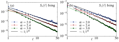
Figure 3: (a) Correlation function $S_{x}(\ell)$ for the long-range Ising model with a random transverse field [$W=5\sin(\pi/5)$] and a constant interaction term ($B=0$) for a system of $L=100$ spins and 50 disorder realizations. (b) Correlation function $S_{z}(\ell)$ for the long-range Ising model with a random interaction [$B=5\sin(\pi/5)$] and a constant magnetic field ($W=0$). In both panels, the power-law tails are fit by the black lines scaling as $1/\ell^{\alpha}$.

Localization of wave functions.— Numerical results on the decay of the single-particle wave functions are obtained by considering the mean value $\Phi(\ell)=\sum_{q=1}^{N}\lvert g_{q,\ell-j_{M}}\rvert/N$ where we average ${N}=L/4$ wave functions $g_{q,\ell}$ with lowest energies, shifted by the quantity $j_{M}$ that corresponds to the lattice site where $\lvert g_{q,\ell}\rvert$ shows its maximum value. We average $\Phi(\ell)$ also over several disorder realizations (of the order of 500).

Figure 4 shows typical results of the decay of $\Phi(\ell)$ as a function of the distance $\ell$ within the localized phases of models (I) and (II) of Eqs. (1) [panels (a,b) and (c,d), respectively].

Remarkably, we find that the wave functions decay algebraically at long distances regardless of the strength $W$ of the disorder, mimicking the scaling of the correlation functions discussed above. However, for all $\alpha$, i.e. both $\alpha>1$ and $\alpha<1$, $\Phi(\ell)$ decays at large distances as $\Phi(\ell)\sim\ell^{-\gamma_{\rm wf}}$, with an exponent $\gamma_{\rm wf}$ consistent with $\gamma_{\rm wf}\sim\alpha$. This is different from the results of Ref. Deng et al. (2018) with positional disorder, where for $\alpha<1$ one gets $\gamma_{\rm wf}\sim 2-\alpha$. For sufficiently large $\alpha>1$ this algebraic decay is preceded by an exponential decay at short distances, reminiscent of the exponentially localized states of short-range random Hamiltonians.

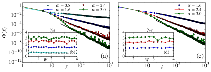
Figure 4: (a) Decay of the averaged wave function $\Phi(\ell)$ (absolute value, see text) of localized states for the model (I): If $\alpha>1$ we find an hybrid exponential and power-law behaviour. If $\alpha<1$ the exponential part is suppressed and only the power-law tail is visible. The black lines correspond to fit of the data scaling as $1/\ell^{\gamma_{\rm wf}}$. (b) Decay exponent $\gamma_{\rm wf}$ for the model (I) of the long-distance tail of $\Phi(\ell)$ as a function of $W$ for different values of $\alpha$. The decay exponent satisfies $\gamma_{\rm wf}\sim\alpha$ and does not show significance dependence on $W$. (c-d) Same as (a-b) but for the model (II) with random long-range pairing.

In summary, we have demonstrated that interactions that decay as a power-law with distance induce an algebraic decay of correlation functions and wave functions both in non-interacting and interacting models in the presence of disorder. This is in stark contrast to results expected from short-range models, and generalises recent results for the decay of wave-functions in quadratic models. These results are of immediate interest for experiments with cold ions, molecule, Rydberg atoms and quantum emitters in cavity fields, to name a few. It is an exciting prospect to explore the properties of many-body quantum phases in the search of exotic transport phenomena with long-range interactions.

P. N.  thanks L. Benini for fruitful discussions. G. P. acknowledges support from ANR “ERA-NET QuantERA” - Projet “RouTe” and UdS via Labex NIE. E. E. is partially supported through the project “QUANTUM” by Istituto Nazionale di Fisica Nucleare (INFN) and through the project “ALMAIDEA” by University of Bologna. The DMRG simulations were performed using the ITensor library ite .

In this Supplemental Material we present details on the numerical simulations and on the analytical derivations related to the $p$-wave superconducting random models that are not shown in the main text. Specifically, in Sec. I we analyze the scaling of the von Neumann entropy that gives further information on the localization properties of the wave functions of model (I). In Sec. II we give the details on the analytical computation of the decay of the single-particle correlation functions, and we show the decay exponents computed numerically. Finally, we show the behavior of the density-density correlation functions.

I Entanglement entropy

In this Section we give further insight on the localization properties of the states of Hamiltonians (I) by analysing the entanglement properties of their eigenmodes.

Measures of entanglement have been widely used to characterise the properties of ground states of many-body quantum systems Vidal et al. (2003) as well as to quantify the degree of localisation for ground- and excited states of disordered models Luitz et al. (2015). A non-trivial measure of the rate of entanglement for a state $\ket{\phi}$ is the von Neumann entropy $S_{\text{vN}}(\phi,\ell)=-\mathrm{Tr}\,\rho_{\ell}\log_{2}\rho_{\ell}$, where $\rho_{\ell}=\mathrm{Tr}\,_{L\setminus\ell}\ket{\phi}\bra{\phi}$ is the reduced density matrix of the state $\ket{\phi}$ that contains $\ell$ sites of the entire lattice. $S_{\text{vN}}$ is known to follow an area-law scaling for localized states $\psi_{\text{loc}}$ [i.e. $S_{\text{vN}}(\psi_{\text{loc}},\ell)\sim\ell^{0}$], while for extended states $\psi_{\text{ext}}$ it it follows a volume law, e.g. it scales as $S_{\text{vN}}(\psi_{\text{ext}},\ell)\sim\ell$ Bauer and Nayak (2013); Li et al. (2015); Geraedts et al. (2016). In the following we compute $S_{\text{vN}}$ semi-analytically for a bipartition of the chain into two equal halves ($\ell=L/2$) for the excited states. An excited state of the Hamiltonians $H_{\text{I,II}}$ is defined by assigning a set of occupied modes $\mathbf{n}=\set{n_{1},n_{2},\ldots,n_{L}}$ with $n_{q}=0,1$ and then creating single quasi-particles $\eta^{\dagger}_{q}$ on the ground state $\ket{\Omega}$ if the mode $q$ is occupied

$$\ket{\mathbf{n}}=\prod_{q=0}^{L-1}[{\eta_{q}^{\dagger}}]^{n_{q}}\ket{\Omega}.$$ (S1)

The two classes of excited states that we consider for computing the von Neumann entropy are given by

$$\ket{\mathbf{n}_{\nu}}=\ket{\underbrace{0\dots 0}_{\nu}\underbrace{11\dots 11}_{L/4}0\dots 0}$$ (S2)

$$\ket{\mathbf{n}^{\prime}_{\nu}}=\ket{\underbrace{0\dots 0}_{\nu}\underbrace{1010\dots 1010}_{L/4}0\dots 0}.$$ (S3)

We study the scaling of the von Neumann entropy as a function of the energy $e(\nu)=\sum_{q}n_{q}\Lambda_{q}$ and the system size $L$.

Following Ref. Peschel (2003), we compute the entropy of the excited states as a function of their energy and, by changing $\nu$, we can explore the whole energy spectrum. This will provide a complete understanding of the different scalings of $S_{\text{vN}}$ with $L$ for high- and low-energy states.

In order to compare the entropies of different eigenmodes, we first rescale the energies by introducing $\epsilon=[e(\nu)-E_{\text{min}}]/(E_{\text{max}}-E_{\text{min}})$, where $E_{\text{min}}$ ($E_{\text{max}}$) is the minimum (maximum) among the energies of the excited states of Eqs. (S2) or (S3). We then average the entropies, after binning them into groups of equal energy width.

In Fig. S1 we show the entanglement entropy of the excited states of Hamiltonian (I) as a function of the system size $L$ for a given choice of $W=1$ and for $\alpha=3$ and $\alpha=0.5$. Panel (a) shows the entropy for the excited states $\ket{\mathbf{n}}$ defined in Eq. (S2) while panel (b) shows the entropy for the excited states $\ket{\mathbf{n}^{\prime}}$ defined in Eq. (S3). For $\alpha=3$, the entropy shows an area-law behavior (i.e., $S_{\text{vN}}\sim L^{0}$) for both the types of excited states at all energies. That behavior can be explained by the localisation of all single-particle modes. For $\alpha=0.5$, instead, the scaling of the entanglement entropy depends on the energy of the excited states $\ket{\mathbf{n}}$ and $\ket{\mathbf{n}^{\prime}}$: it goes from approximately constant for the low-energy states (depicted in blue), while it is found to follow a volume law (i.e., $S_{\text{vN}}\sim L$) for the high-energy ones (depicted with green lines). We notice that the changing in the behavior of the entropy from area law to volume law is enhanced for the states $\ket{\mathbf{n}^{\prime}}$. This behaviour is compatible with the presence of a mobility edge for all $\alpha<1$ that separates localized low-energy states from extended high-energy ones.

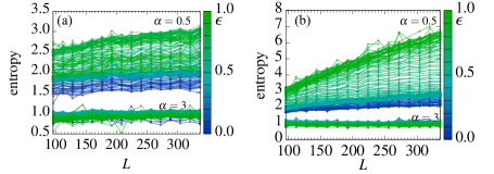
Figure S1: von Neumann entropy $S_{\text{vN}}$ for the many-particle excited states of Hamiltonian (I) as a function of the system size $L$ for different energies $\epsilon$ and $W=1$: (a) states $\ket{\mathbf{n}}$ from Eq. (S2), (b) states $\ket{\mathbf{n}^{\prime}}$ from Eq. (S3). For $\alpha=3.0$, as all single-particle modes are localized, the entropy of the states for all energies does not depend on the system size (i.e the von Neumann entropy satisfies an area law). For $\alpha=0.5$, the scaling of the entanglement entropy depends on the energy of the excited states $\ket{\mathbf{n}}$ and $\ket{\mathbf{n}^{\prime}}$: it goes from approximately constant for the low-energy states (depicted in blue), while it is found to follow a volume law (i.e., $S_{\text{vN}}\sim L$) for the high-energy ones (depicted with green lines).

II Decay of correlation functions

In this Section we show how to compute the correlation function $C(j,i)=\braket{a^{\dagger}_{j}a_{i}}$ by perturbation theory. We will discuss only the model with random hopping, as the one with random long-range pairing can be treated similarly.

II.1 Correlation functions - Perturbation theory

We recall that the Hamiltonian $H_{\rm I}$ in Eq. (1) of the main text is formed by two parts:

$$H_{{\rm I}}=H_{0}+V_{{\rm I}}$$ (S4)

where

$$H_{0}=-t\sum_{j=1}^{L}\left(a^{\dagger}_{j}a_{j+1}+\mathrm{H.c.}\right)+\mu\sum_{j=1}^{L}a^{\dagger}_{j}a_{j}+\sum_{j,\ell}\frac{\Delta}{\ell^{\alpha}}\left(a_{j}a_{j+\ell}+\mathrm{H.c.}\right),$$ (S5)

and

$$V_{\rm I}=-t\sum_{j=1}^{L}W_{j}\left(a^{\dagger}_{j}a_{j+1}+\mathrm{H.c.}\right).$$ (S6)

In order to compute the correlation function $C(j,i)=\braket{\Omega}{a^{\dagger}_{j}a_{i}}{\Omega}$ on the ground state $\ket{\Omega}$ of $H_{\text{I}}$ in Eq. (S4), we first find the first-order correction $\ket{\delta\Omega_{0}}$ to the ground state $\ket{\Omega_{0}}$ of $H_{0}$ by treating $V_{\text{I}}$ as a perturbation.

The first-order correction $\ket{\delta\Omega_{0}}$ to the ground state $\ket{\Omega_{0}}$ of the Hamiltonian $H_{0}$ due to the perturbation $V_{\text{I}}$ is given by Sakurai and Napolitano (2011)

$$\ket{\delta\Omega_{0}}=\sum_{\mathbf{n}_{0}}\frac{\braket{\mathbf{n}_{0}}{V_{\text{I}}}{\Omega_{0}}}{E(\mathbf{n}_{0})-E_{0}}\ket{\mathbf{n}_{0}}$$ (S7)

where, the quantities $E(\mathbf{n}_{0})$ and $E_{0}$ are the energy of the states $\ket{\mathbf{n}_{0}}$ and of $\ket{\Omega_{0}}$, respectively and $\ket{\mathbf{n}_{0}}$ indicates an excited state of the homogeneous Hamiltonian $H_{0}$ that can be diagonalized via Fourier and Bogoliubov transformations as

$$H_{0}=\sum_{k}\lambda_{\alpha}(k)\xi^{\dagger}_{k}\xi_{k}.$$ (S8)

The ground state $\ket{\Omega_{0}}$ of $H_{0}$ is then the vacuum of all quasi-particles $\xi_{k}$.

In Eq. (S8) we have defined the single-particle energy

$$\lambda_{\alpha}(k)=[\left(\cos k-\mu\right)^{2}+4f_{\alpha}^{2}(k)]^{1/2}$$ (S9)

and the Bogolioubov quasi-particles $\xi_{k}$ that are related to the original fermionic operators $\tilde{a}_{k}$ in momentum space via

$$\tilde{a}_{k}=v_{k}\xi_{k}-u_{k}\xi^{\dagger}_{-k}$$ (S10)

with $v_{k}=\cos\varphi(k)$ and $u_{k}=\mathrm{i}\sin\varphi(k)$ where $\tan 2\varphi(k)=f_{\alpha}(k)/[\mu-\cos k]$ and $f_{\alpha}(k)=\sum_{\ell=1}^{L-1}\sin(k\ell)/\ell^{\alpha}$. We notice that the functions $f_{\alpha}(k)$ when $L\to\infty$ become $f_{\alpha}(k)=\left[\mathrm{Li}_{\alpha}\!(\text{e}^{\mathrm{i}k})-\mathrm{Li}_{\alpha}\!(\text{e}^{-\mathrm{i}k})\right]/(2\mathrm{i})$, with $\mathrm{Li}_{\alpha}\!(z)=\sum_{j}z^{j}/j^{\alpha}$ a polylogarithm of order $\alpha$.

The excited states $\ket{\mathbf{n}_{0}}$ are defined by assigning a set of occupied modes $\mathbf{n}_{0}=\set{n_{1},n_{2},\ldots,n_{L}}$ with $n_{q}=0,1$ and then creating single quasi-particles $\xi^{\dagger}_{q}$ on the ground state $\ket{\Omega_{0}}$ if the mode $q$ is occupied

$$\ket{\mathbf{n}_{0}}=\prod_{q=0}^{L-1}[{\xi_{q}^{\dagger}}]^{n_{q}}\ket{\Omega_{0}}.$$ (S11)

The first-order correction $\ket{\delta\Omega_{0}}$ can now be obtained from Eq. (S7) that gives

$$\ket{\Omega}=\ket{\Omega_{0}}+\ket{\delta\Omega_{0}}=\ket{\Omega_{0}}-\sum_{kk^{\prime}}{J}_{k,k^{\prime}}A(k,k^{\prime})\xi^{\dagger}_{k}\xi^{\dagger}_{k^{\prime}}\ket{\Omega_{0}},$$ (S12)

where we have defined ${J}_{k,k^{\prime}}=-\sum_{j}e^{\mathrm{i}(k-k^{\prime})j}W_{j}/L$ and $A(k,k^{\prime})=2(\text{e}^{\mathrm{i}k}+\text{e}^{-\mathrm{i}k^{\prime}})v_{k}u^{*}_{k^{\prime}}/[\lambda(k)+\lambda(k^{\prime})]$.

On a single disorder realization the correlation function $\braket{\Omega}{a^{\dagger}_{j}a_{i}}{\Omega}$ takes the form

$$\braket{\Omega}{a^{\dagger}_{j}a_{i}}{\Omega}=\braket{\Omega_{0}}{a^{\dagger}_{j}a_{i}}{\Omega_{0}}+\braket{\delta\Omega_{0}}{a^{\dagger}_{j}a_{i}}{\Omega_{0}}+\braket{\Omega_{0}}{a^{\dagger}_{j}a_{i}}{\delta\Omega_{0}}+\braket{\delta\Omega_{0}}{a^{\dagger}_{j}a_{i}}{\delta\Omega_{0}}.$$ (S13)

If we now average Eq. (S13) over many disorder realizations, the cross terms $\braket{\delta\Omega_{0}}{a^{\dagger}_{j}a_{i}}{\Omega_{0}}$ and $\braket{\Omega_{0}}{a^{\dagger}_{j}a_{i}}{\delta\Omega_{0}}$ vanish as, due to the correction $\ket{\delta\Omega_{0}}$, only one random term $W_{j}$ (that has mean value zero) appears in them. Therefore we get

$$\braket{\Omega}{a^{\dagger}_{j}a_{i}}{\Omega}_{W}=\braket{\Omega_{0}}{a^{\dagger}_{j}a_{i}}{\Omega_{0}}+\braket{\delta\Omega_{0}}{a^{\dagger}_{j}a_{i}}{\delta\Omega_{0}}_{W}.$$ (S14)

The first term of the r.h.s. of Eq. (S14) corresponds to the correlator for a homogenous translationally-invariant system. By rewriting $a^{\dagger}_{j}$ and $a_{i}$ in momentum space and by using Eq. (S10) recalling that $\xi_{k}\ket{\Omega_{0}}=0$ we obtain

$$C_{0}(\ell):=\braket{\Omega_{0}}{a^{\dagger}_{j}a_{i}}{\Omega_{0}}=\frac{1}{L}\sum_{k}\text{e}^{\mathrm{i}k\ell}R_{0}(k)$$ (S15)

where $\ell=j-i$ and $R_{0}(k)=\lvert u_{k}\rvert^{2}$.

In the second term of the r.h.s. of Eq. (S14), as we are averaging on the disorder configurations, we can expect that the disorder average $\braket{\delta\Omega_{0}}{a^{\dagger}_{j}a_{i}}{\delta\Omega_{0}}_{W}$ will be translationally invariant, i.e. it will depend on the relative distance $\ell=j-i$ while the terms that depend on $i$ and $j$ separately will average out to zero (see §6.5 in Ref. Altland and Simons (2006) or §12.3 in Ref. Bruus and Flensberg (2004)). By keeping only the terms that depend on $\ell$, after rewriting $a^{\dagger}_{j}$ and $a_{i}$ in momentum space and using again Eq. (S10) recalling that $\xi_{k}\ket{\Omega_{0}}=0$, the second term becomes

$$C_{1}(\ell):=\braket{\delta\Omega_{0}}{a^{\dagger}_{j}a_{i}}{\delta\Omega_{0}}_{W}=\frac{W^{2}}{3L}\sum_{k}\text{e}^{\mathrm{i}k\ell}R_{1}(k)$$ (S16)

where

$$R_{1}(k) =c\lvert u_{k}\rvert^{2}+U(k)\lvert u_{k}\rvert^{2}-V(k)\lvert v_{k}\rvert^{2},\phantom{\sum_{p}}$$ (S17)

$$c =\sum_{p}A(p,p)^{2}-\sum_{p_{1}p_{2}}A(p_{1},p_{2})A(p_{2},p_{1}),$$ (S18)

$$U(k) =2\sum_{p}A(p,-k)A(-k,p)=-\frac{f_{\alpha}(k)}{\lambda_{\alpha}(k)}\sum_{p}\frac{2+2\cos(p-k)}{(\lambda_{\alpha}(k)+\lambda_{\alpha}(p))^{2}}\frac{f_{\alpha}(p)}{\lambda_{\alpha}(p)},$$ (S19)

$$V(k) =2\sum_{p}A(p,k)A(k,p)=\frac{f_{\alpha}(k)}{\lambda_{\alpha}(k)}\sum_{p}\frac{2+2\cos(p+k)}{(\lambda_{\alpha}(k)+\lambda_{\alpha}(p))^{2}}\frac{f_{\alpha}(p)}{\lambda_{\alpha}(p)}.$$ (S20)

We note that the quantity $c$ does not depend on $k$.

II.2 Correlation functions - Asymptotic behavior

Figure S2: Integration contour for evaluating the asymptotic behaviors of the correlators $C_{0}(\ell)$ in Eq. (S24) and $C_{1}(\ell)$ in Eq. (S30).

In this Section we show how the two correlators $C_{0}(\ell)$ and $C_{1}(\ell)$ behave asymptotically for $\ell\to\infty$.

Let us consider $C_{0}(\ell)$ in Eq. (S15) first. In the limit $L\to\infty$ we can replace the summation with an integral

$$C_{0}(\ell)=\frac{1}{2\pi}\int_{-\infty}^{\infty}\mathrm{d}k\ \text{e}^{\mathrm{i}k\ell}R_{0}(k).$$ (S21)

The asymptotic behavior of $C_{0}(\ell)$ for $\ell\to\infty$ can be computed by considering the integrals $I_{0}^{+}$ and $I_{0}^{-}$ on the complex plane in Fig. S2 that are

$$I_{0}^{+}=\frac{1}{2\pi}\int_{s_{+}}\mathrm{d}z\ \text{e}^{\mathrm{i}z\ell}R_{0}(z)+\frac{1}{2\pi}\int_{\Gamma_{+}}\mathrm{d}z\ \text{e}^{\mathrm{i}z\ell}R_{0}(z)+\frac{1}{2\pi}\int_{0}^{\infty}\mathrm{d}k\ \text{e}^{\mathrm{i}k\ell}R_{0}(k)$$ (S22)

$$I_{0}^{-}=\frac{1}{2\pi}\int_{s_{-}}\mathrm{d}z\ \text{e}^{\mathrm{i}z\ell}R_{0}(z)+\frac{1}{2\pi}\int_{\Gamma_{-}}\mathrm{d}z\ \text{e}^{\mathrm{i}z\ell}R_{0}(z)+\frac{1}{2\pi}\int_{-\infty}^{0}\mathrm{d}k\ \text{e}^{\mathrm{i}k\ell}R_{0}(k)$$ (S23)

where we have chosen to put the branch cut of the complex logarithm [see the expansion of the polylogarithm in Eq. (S25)] on the imaginary positive axis.

By sending the radius $r$ of the circles $\Gamma_{\pm}$ to infinity and by neglecting possible residues inside the integration contour that will contribute only with exponential decaying terms we have

$$\begin{split}C_{0}(\ell)&=-\frac{1}{2\pi}\int_{s_{+}}\mathrm{d}z\ \text{e}^{\mathrm{i}z\ell}R_{0}(z)-\frac{1}{2\pi}\int_{s_{-}}\mathrm{d}z\ \text{e}^{\mathrm{i}z\ell}R_{0}(z)\\ &=\frac{\mathrm{i}}{2\pi}\int_{0}^{\infty}\mathrm{d}y\ \text{e}^{-y\ell}R_{0}(\epsilon+\mathrm{i}y)-\frac{\mathrm{i}}{2\pi}\int_{-\infty}^{0}\mathrm{d}y\ \text{e}^{-y\ell}R_{0}(-\epsilon+\mathrm{i}y)\\ &=\frac{1}{\pi}\int_{0}^{\infty}\mathrm{d}y\ \text{e}^{-y\ell}\mathop{\text{Im}}\nolimits R_{0}(\mathrm{i}y)\end{split}$$ (S24)

where on the lines $s_{\pm}$ the complex variable is $z=\pm\epsilon+\mathrm{i}y$ with $\epsilon$ a small positive parameter that we send to zero.

We are able now to evaluate the asymptotic behavior of $C_{0}(\ell)$ by computing the $y\to 0$ part of $\mathop{\text{Im}}\nolimits[R_{0}(\mathrm{i}y)]$ and then integrating the last equality in Eq. (S24). This is done by recalling that the polylogarithm admits the series expansion Abramowitz and Stegun (1964); Olver et al. (2010) for a general complex number $z$ as

$$\operatorname{Li}_{\alpha}(z)=\Gamma(1-\alpha)\left(\ln\frac{1}{z}\right)^{\alpha-1}+\sum_{n=0}^{\infty}\zeta(\alpha-n)\frac{(\ln z)^{n}}{n!}$$ (S25)

that makes them non-analytical due to the presence of the complex logarithm and the power-law. In Eq. (S25), $\Gamma(x)$ and $\zeta(x)$ are the Euler gamma function and the Riemann zeta function, respectively.

By using the series expansion of the polylogarithms from Eq. (S25) that yields

$$\mathrm{Li}_{\alpha}\!(\text{e}^{-y})-\mathrm{Li}_{\alpha}\!(\text{e}^{y})=\Gamma(1-\alpha)\left(1+\text{e}^{\mathrm{i}\pi\alpha}\right)y^{\alpha-1}-2\sum_{n\text{ odd}}^{\infty}\frac{\zeta(\alpha-n)}{n!}y^{n}$$ (S26)

we can obtain the function $R_{0}(\mathrm{i}y)$ on the imaginary axis:

$$R_{0}(\mathrm{i}y)=\frac{\mu-\cosh y}{2\lambda_{\alpha}(\mathrm{i}y)}\sim\frac{\mu-1}{2\sqrt{(\mu-1)^{2}-\Gamma^{2}(1-\alpha)(\text{e}^{\mathrm{i}\pi\alpha}+1)^{2}y^{2\alpha-2}-4\Gamma(1-\alpha)(\text{e}^{\mathrm{i}\pi\alpha}+1)\zeta(\alpha-1)y^{\alpha}}}.$$ (S27)

The previous equation in the limit $y\to 0$ gives

$$\mathop{\text{Im}}\nolimits R_{0}(\mathrm{i}y)=\begin{cases}y^{1-\alpha}&\text{for }\alpha<1\\ y^{2\alpha-2}&\text{for }1<\alpha<2\\ y^{\alpha}&\text{for }\alpha>2\end{cases}$$ (S28)

and, after performing the last integral in Eq. (S24), the asymptotic behavior of $C_{0}$ turns out to be

$$C_{0}(\ell)\sim\begin{cases}{1}/{\ell^{2-\alpha}}&\text{for }\alpha<1\\ {1}/{\ell^{2\alpha-1}}&\text{for }1<\alpha<2\\ {1}/{\ell^{\alpha+1}}&\text{for }\alpha>2.\end{cases}$$ (S29)

For the correlator $C_{1}(\ell)$ in Eq. (S16) we can use the same contour in Fig. S2 and get

$$C_{1}(\ell)=\frac{W^{2}}{3\pi}\int_{0}^{\infty}\mathrm{d}y\ \text{e}^{-y\ell}\mathop{\text{Im}}\nolimits R_{1}(\mathrm{i}y).$$ (S30)

For the asymptotic behaviour of $C_{1}(\ell)$, we need again the $y\to 0$ part of $R_{1}(\mathrm{i}y)$. Let us start by noting that from Eqs. (S19) and (S20) the $y\to 0$ part of both $U(\mathrm{i}y)$ and $V(\mathrm{i}y)$ is given by

$$\mathop{\text{Im}}\nolimits[U(\mathrm{i}y)\lvert u_{\mathrm{i}y}\rvert^{2}]\sim\mathop{\text{Im}}\nolimits[V(\mathrm{i}y)\lvert v_{\mathrm{i}y}\rvert^{2}]\sim\mathop{\text{Im}}\nolimits\frac{f_{\alpha}(\mathrm{i}y)(\mu-\cosh y)}{\lambda^{2}_{\alpha}(\mathrm{i}y)}\sim\begin{cases}y^{1-\alpha}&\text{for }\alpha<1\\ y^{\alpha-1}&\text{for }\alpha>1.\end{cases}$$ (S31)

The previous equation, by considering also the contribution coming from $c\lvert u_{\mathrm{i}y}\rvert^{2}$ [see Eq. (S17)], gives

$$\mathop{\text{Im}}\nolimits R_{1}(\mathrm{i}y)\sim\begin{cases}y^{1-\alpha}&\text{for }\alpha<1\\ y^{\alpha-1}&\text{for }\alpha>1\end{cases}$$ (S32)

and after integrating Eq. (S30), we finally get the correlator

$$C_{1}(\ell)=\begin{cases}{W^{2}}/{\ell^{2-\alpha}}&\text{for }\alpha<1\\ {W^{2}}/{\ell^{\alpha}}&\text{for }\alpha>1.\end{cases}$$ (S33)

The asymptotic behavior coming from Eqs. (S29), (S33) can be checked by computing the correlator $C(\ell)$ numerically as reported in Fig. 2(a) of the main text. Remarkably, the values of the decay exponents of the power-law tails do not depend on the disorder strength $W$ as shown in Fig. S3 where we plot the decay exponents of $C(\ell)$ as a function of $W$ for different values of $\alpha$. For completeness we show also the decay exponent of the correlation function $C(\ell)$ for the model (II) with random long-range pairing.

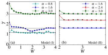
Figure S3: (a) Decay exponent $\gamma$ of the long-distance tail of the correlation function $C(\ell)$ for the model (I) as a function of $W$ and for $\alpha=0.8$ (cyan triangles), $\alpha=1.6$ (blue circles), $\alpha=3.0$ (green diamonds). If $W>0$, the decay exponent satisfies $\gamma\sim\alpha$ for $\alpha>1$ and $\gamma\sim 2-\alpha$ for $\alpha<1$ and it does not show significance dependence on $W$. These data are obtained by computing the correlation function $C(\ell)$ numerically from the full random Hamiltonian in Eq. (S4) and then by fitting the long-range decaying tail of $C(\ell)$ with $1/\ell^{\gamma}$. The black lines represent the expected exponents: $\gamma=1.2$ for $\alpha=0.8$, $\gamma=1.6$ for $\alpha=1.6$, $\gamma=3.0$ for $\alpha=3.0$. (b) Same as panel (a) but for the localized phase (for $W\gtrsim 2$) of model (II).

II.3 Density-density correlation function

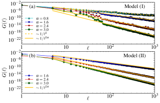
Figure S4: (a) Density-density correlation function $G(\ell)$ for the model (I) as a function of the lattice site $\ell$ for different values of $\alpha$ and for $W=5$, $L=2000$ and 400 disorder realizations. The power-law tails are fit by the yellow lines scaling as $1/\ell^{2}$ (dashed) and $1/\ell^{2\alpha}$ (solid). (b) Same as panel (a) but for the model (II).

From the single-particle correlators $\braket{a^{\dagger}_{j}a_{j+\ell}}$ and $\braket{a^{\dagger}_{j}a^{\dagger}_{j+\ell}}$, by means of the Wick theorem, we computed also the density-density correlation functions $G(j,\ell)=\left[\braket{n_{j}n_{j+\ell}}-\braket{n_{j}}\braket{n_{j+\ell}}\right]_{W}=[\lvert\braket{a_{j}a_{j+\ell}}\rvert^{2}-\lvert\braket{a^{\dagger}_{j}a_{j+\ell}}\rvert^{2}]_{W}$.

Examples of $G(\ell)=G(j_{0},\ell)$ with $j_{0}=L/4$ are shown in Fig. S4 for a system of $L=2000$ sites and for a disorder strength $W=5$. Numerically we find that in the localized phases for model (I) when $\alpha<1$, $G(\ell)\sim 1/\ell^{2}$ while for both models $G(\ell)\sim 1/\ell^{2\alpha}$ when $\alpha>1$. The first behaviour with a decay exponent that does not depend on $\alpha$ has been already observed in Refs. Vodola et al. (2014, 2016), while the second can be explained by looking at the $\ell\to\infty$ scaling of $\lvert C(\ell)\rvert^{2}\sim 1/\ell^{2\alpha}$ in Eq. (S33).

References

- Anderson (1958) P. W. Anderson, “Absence of diffusion in certain random lattices,” Phys. Rev. 109, 1492 (1958)\BibitemShutNoStop
- Roati et al. (2008) G. Roati, C. D’Errico, L. Fallani, M. Fattori, C. Fort, M. Zaccanti, G. Modugno, M. Modugno, and M. Inguscio, “Anderson localization of a non-interacting Bose-Einstein condensate,” Nature (London) 453, 895 (2008)\BibitemShutNoStop
- Billy et al. (2008) J. Billy, V. Josse, Z. Zuo, A. Bernard, B. Hambrecht, P. Lugan, D. Clement, L. Sanchez-Palencia, P. Bouyer, and A. Aspect, “Direct observation of Anderson localization of matter waves in a controlled disorder,” Nature (London) 453, 891 (2008)\BibitemShutNoStop
- Kondov et al. (2011) S. S. Kondov, W. R. McGehee, J. J. Zirbel, and B. DeMarco, “Three-dimensional Anderson localization of ultracold matter,” Science 334, 66 (2011)\BibitemShutNoStop
- Jendrzejewski et al. (2012) F. Jendrzejewski, A. Bernard, K. Muller, P. Cheinet, V. Josse, M. Piraud, L. Pezze, L. Sanchez-Palencia, A. Aspect, and P. Bouyer, “Three-dimensional localization of ultracold atoms in an optical disordered potential,” Nat. Phys. 8, 398 (2012)\BibitemShutNoStop
- Schreiber et al. (2015) M. Schreiber, S. S. Hodgman, P. Bordia, H. P. Lüschen, M. H. Fischer, R. Vosk, E. Altman, U. Schneider, and I. Bloch, “Observation of many-body localization of interacting fermions in a quasirandom optical lattice,” Science 349, 842 (2015)\BibitemShutNoStop
- Smith et al. (2016) J. Smith, A. Lee, P. Richerme, B. Neyenhuis, P. W. Hess, P. Hauke, M. Heyl, D. A. Huse, and C. Monroe, “Many-body localization in a quantum simulator with programmable random disorder,” Nat. Phys. 12, 907 (2016)\BibitemShutNoStop
- Bordia et al. (2016) P. Bordia, H. P. Lüschen, S. S. Hodgman, M. Schreiber, I. Bloch, and U. Schneider, “Coupling Identical one-dimensional Many-Body Localized Systems,” Phys. Rev. Lett. 116, 140401 (2016)\BibitemShutNoStop
- Lee and Ramakrishnan (1985) P. A. Lee and T. V. Ramakrishnan, “Disordered electronic systems,” Rev. Mod. Phys. 57, 287 (1985)\BibitemShutNoStop
- Altshuler et al. (1997) B. L. Altshuler, Y. Gefen, A. Kamenev, and L. S. Levitov, “Quasiparticle lifetime in a finite system: A nonperturbative approach,” Phys. Rev. Lett. 78, 2803 (1997)\BibitemShutNoStop
- Basko et al. (2006) D. Basko, I. Aleiner, and B. Altshuler, “Metal–insulator transition in a weakly interacting many-electron system with localized single-particle states,” Ann. Phys. 321, 1126 (2006)\BibitemShutNoStop
- Oganesyan and Huse (2007) V. Oganesyan and D. A. Huse, “Localization of interacting fermions at high temperature,” Phys. Rev. B 75, 155111 (2007)\BibitemShutNoStop
- Gornyi et al. (2005) I. V. Gornyi, A. D. Mirlin, and D. G. Polyakov, “Interacting Electrons in Disordered Wires: Anderson Localization and Low-T Transport,” Phys. Rev. Lett. 95, 206603 (2005)\BibitemShutNoStop
- Žnidarič et al. (2008) M. Žnidarič, T. Prosen, and P. Prelovšek, “Many-body localization in the Heisenberg magnet in a random field,” Phys. Rev. B 77, 064426 (2008)\BibitemShutNoStop
- Biddle et al. (2009) J. Biddle, B. Wang, D. J. Priour, and S. Das Sarma, “Localization in one-dimensional incommensurate lattices beyond the Aubry-André model,” Phys. Rev. A 80, 021603 (2009)\BibitemShutNoStop
- Biddle and Das Sarma (2010) J. Biddle and S. Das Sarma, “Predicted mobility edges in one-dimensional incommensurate optical lattices: An exactly solvable model of Anderson localization,” Phys. Rev. Lett. 104, 070601 (2010)\BibitemShutNoStop
- Biddle et al. (2011) J. Biddle, D. J. Priour, B. Wang, and S. Das Sarma, “Localization in one-dimensional lattices with non-nearest-neighbor hopping: Generalized Anderson and Aubry-André models,” Phys. Rev. B 83, 075105 (2011)\BibitemShutNoStop
- Pal and Huse (2010) A. Pal and D. A. Huse, “Many-body localization phase transition,” Phys. Rev. B 82, 174411 (2010)\BibitemShutNoStop
- Luca and Scardicchio (2013) A. D. Luca and A. Scardicchio, “Ergodicity breaking in a model showing many-body localization,” EPL (Europhys. Lett.) 101, 37003 (2013)\BibitemShutNoStop
- Vosk and Altman (2013) R. Vosk and E. Altman, “Many-Body Localization in One Dimension as a Dynamical Renormalization Group Fixed Point,” Phys. Rev. Lett. 110, 067204 (2013)\BibitemShutNoStop
- Bar Lev and Reichman (2014) Y. Bar Lev and D. R. Reichman, “Dynamics of many-body localization,” Phys. Rev. B 89, 220201 (2014)\BibitemShutNoStop
- Bar Lev et al. (2015) Y. Bar Lev, G. Cohen, and D. R. Reichman, “Absence of Diffusion in an Interacting System of Spinless Fermions on a One-Dimensional Disordered Lattice,” Phys. Rev. Lett. 114, 100601 (2015)\BibitemShutNoStop
- Luitz et al. (2015) D. J. Luitz, N. Laflorencie, and F. Alet, “Many-body localization edge in the random-field Heisenberg chain,” Phys. Rev. B 91, 081103 (2015)\BibitemShutNoStop
- Luitz (2016) D. J. Luitz, “Long tail distributions near the many-body localization transition,” Phys. Rev. B 93, 134201 (2016)\BibitemShutNoStop
- Naldesi et al. (2016) P. Naldesi, E. Ercolessi, and T. Roscilde, “Detecting a many-body mobility edge with quantum quenches,” SciPost Phys. 1, 010 (2016)\BibitemShutNoStop
- Nandkishore et al. (2014) R. Nandkishore, S. Gopalakrishnan, and D. A. Huse, “Spectral features of a many-body-localized system weakly coupled to a bath,” Phys. Rev. B 90, 064203 (2014)\BibitemShutNoStop
- Gornyi et al. (2017) I. V. Gornyi, A. D. Mirlin, M. Müller, and D. G. Polyakov, “Absence of many-body localization in a continuum,” Annalen der Physik 529, 1600365 (2017)\BibitemShutNoStop
- Potter and Vasseur (2016) A. C. Potter and R. Vasseur, “Symmetry constraints on many-body localization,” Phys. Rev. B 94, 224206 (2016)\BibitemShutNoStop
- Kastner (2010) M. Kastner, “Nonequivalence of ensembles for long-range quantum spin systems in optical lattices,” Phys. Rev. Lett. 104, 240403 (2010)\BibitemShutNoStop
- Gong et al. (2014) Z.-X. Gong, M. Foss-Feig, S. Michalakis, and A. V. Gorshkov, “Persistence of locality in systems with power-law interactions,” Phys. Rev. Lett. 113, 030602 (2014)\BibitemShutNoStop
- Foss-Feig et al. (2015) M. Foss-Feig, Z.-X. Gong, C. W. Clark, and A. V. Gorshkov, “Nearly Linear Light Cones in Long-Range Interacting Quantum Systems,” Phys. Rev. Lett. 114, 157201 (2015)\BibitemShutNoStop
- Hauke and Tagliacozzo (2013) P. Hauke and L. Tagliacozzo, “Spread of correlations in long-range interacting quantum systems,” Phys. Rev. Lett. 111, 207202 (2013)\BibitemShutNoStop
- Eisert et al. (2013) J. Eisert, M. van den Worm, S. R. Manmana, and M. Kastner, “Breakdown of quasilocality in long-range quantum lattice models,” Phys. Rev. Lett. 111, 260401 (2013)\BibitemShutNoStop
- Schachenmayer et al. (2013) J. Schachenmayer, B. P. Lanyon, C. F. Roos, and A. J. Daley, “Entanglement growth in quench dynamics with variable range interactions,” Phys. Rev. X 3, 031015 (2013)\BibitemShutNoStop
- Métivier et al. (2014) D. Métivier, R. Bachelard, and M. Kastner, “Spreading of perturbations in long-range interacting classical lattice models,” Phys. Rev. Lett. 112, 210601 (2014)\BibitemShutNoStop
- Kastner and van den Worm (2015) M. Kastner and M. van den Worm, “Relaxation timescales and prethermalization in d -dimensional long-range quantum spin models,” Physica Scripta 2015, 014039 (2015)\BibitemShutNoStop
- Cevolani et al. (2015) L. Cevolani, G. Carleo, and L. Sanchez-Palencia, “Protected quasilocality in quantum systems with long-range interactions,” Phys. Rev. A 92, 041603 (2015)\BibitemShutNoStop
- Cevolani et al. (2016) L. Cevolani, G. Carleo, and L. Sanchez-Palencia, “Spreading of correlations in exactly solvable quantum models with long-range interactions in arbitrary dimensions,” New Journal of Physics 18, 093002 (2016)\BibitemShutNoStop
- Bettles et al. (2017) R. J. Bettles, J. Minář, C. S. Adams, I. Lesanovsky, and B. Olmos, “Topological properties of a dense atomic lattice gas,” Phys. Rev. A 96, 041603 (2017)\BibitemShutNoStop
- Frérot et al. (2017) I. Frérot, P. Naldesi, and T. Roscilde, “Entanglement and fluctuations in the XXZ model with power-law interactions,” Phys. Rev. B 95, 245111 (2017)\BibitemShutNoStop
- Frérot et al. (2018) I. Frérot, P. Naldesi, and T. Roscilde, “Multispeed prethermalization in quantum spin models with power-law decaying interactions,” Phys. Rev. Lett. 120, 050401 (2018)\BibitemShutNoStop
- Schneider et al. (2012) C. Schneider, D. Porras, and T. Schätz, “Experimental quantum simulations of many-body physics with trapped ions,” Reports on Progress in Physics 75, 024401 (2012)\BibitemShutNoStop
- Richerme et al. (2014) P. Richerme, Z.-X. Gong, A. Lee, C. Senko, J. Smith, M. Foss-Feig, S. Michalakis, A. V. Gorshkov, and C. Monroe, “Non-local propagation of correlations in quantum systems with long-range interactions,” Nature (London) 511, 198 (2014)\BibitemShutNoStop
- Jurcevic et al. (2014) P. Jurcevic, B. P. Lanyon, P. Hauke, C. Hempel, P. Zoller, R. Blatt, and C. F. Roos, “Quasiparticle engineering and entanglement propagation in a quantum many-body system,” Nature (London) 511, 202 (2014)\BibitemShutNoStop
- Britton et al. (2012) J. W. Britton, B. C. Sawyer, A. C. Keith, C. C. J. Wang, J. K. Freericks, H. Uys, M. J. Biercuk, and J. J. Bollinger, “Engineered two-dimensional Ising interactions in a trapped-ion quantum simulator with hundreds of spins,” Nature (London) 484, 489 (2012)\BibitemShutNoStop
- Bermudez et al. (2013) A. Bermudez, T. Schäetz, and M. B. Plenio, “Dissipation-assisted quantum information processing with trapped ions,” Phys. Rev. Lett. 110, 110502 (2013)\BibitemShutNoStop
- Shahmoon and Kurizki (2013) E. Shahmoon and G. Kurizki, “Nonradiative interaction and entanglement between distant atoms,” Phys. Rev. A 87, 033831 (2013)\BibitemShutNoStop
- Douglas et al. (2015) J. S. Douglas, H. Habibian, C. L. Hung, A. V. Gorshkov, H. J. Kimble, and D. E. Chang, “Quantum many-body models with cold atoms coupled to photonic crystals,” Nat. Photonics 9, 326 (2015)\BibitemShutNoStop
- Litinskaya et al. (2016) M. Litinskaya, E. Tignone, and G. Pupillo, “Broadband photon-photon interactions mediated by cold atoms in a photonic crystal fiber,” Scientific Reports 6, 25630 (2016)\BibitemShutNoStop
- Vaidya et al. (2018) V. D. Vaidya, Y. Guo, R. M. Kroeze, K. E. Ballantine, A. J. Kollár, J. Keeling, and B. L. Lev, “Tunable-Range, Photon-Mediated Atomic Interactions in Multimode Cavity QED,” Phys. Rev. X 8, 011002 (2018)\BibitemShutNoStop
- Kadau et al. (2016) H. Kadau, M. Schmitt, M. Wenzel, C. Wink, T. Maier, I. Ferrier-Barbut, and T. Pfau, “Observing the Rosensweig instability of a quantum ferrofluid,” Nature 530, 194 EP (2016)\BibitemShutNoStop
- Lepoutre et al. (2018) S. Lepoutre, L. Gabardos, K. Kechadi, P. Pedri, O. Gorceix, E. Maréchal, L. Vernac, and B. Laburthe-Tolra, “Collective spin modes of a trapped quantum ferrofluid,” Phys. Rev. Lett. 121, 013201 (2018)\BibitemShutNoStop
- Baier et al. (2018) S. Baier, D. Petter, J. H. Becher, A. Patscheider, G. Natale, L. Chomaz, M. J. Mark, and F. Ferlaino, “Realization of a strongly interacting Fermi gas of dipolar atoms,” Phys. Rev. Lett. 121, 093602 (2018)\BibitemShutNoStop
- Tang et al. (2018) Y. Tang, W. Kao, K.-Y. Li, and B. L. Lev, “Tuning the dipole-dipole interaction in a quantum gas with a rotating magnetic field,” Phys. Rev. Lett. 120, 230401 (2018)\BibitemShutNoStop
- Weimer et al. (2008) H. Weimer, R. Löw, T. Pfau, and H. P. Büchler, “Quantum critical behavior in strongly interacting Rydberg gases,” Phys. Rev. Lett. 101, 250601 (2008)\BibitemShutNoStop
- Saffman et al. (2010) M. Saffman, T. G. Walker, and K. Mølmer, “Quantum information with Rydberg atoms,” Rev. Mod. Phys. 82, 2313 (2010)\BibitemShutNoStop
- Viteau et al. (2012) M. Viteau, P. Huillery, M. G. Bason, N. Malossi, D. Ciampini, O. Morsch, E. Arimondo, D. Comparat, and P. Pillet, “Cooperative excitation and many-body interactions in a cold Rydberg gas,” Phys. Rev. Lett. 109, 053002 (2012)\BibitemShutNoStop
- Schauß et al. (2012) P. Schauß, M. Cheneau, M. Endres, T. Fukuhara, S. Hild, A. Omran, T. Pohl, C. Gross, S. Kuhr, and I. Bloch, “Observation of spatially ordered structures in a two-dimensional Rydberg gas,” Nature (London) 491, 87 (2012)\BibitemShutNoStop
- Carr et al. (2013) C. Carr, R. Ritter, C. G. Wade, C. S. Adams, and K. J. Weatherill, “Nonequilibrium phase transition in a dilute Rydberg ensemble,” Phys. Rev. Lett. 111, 113901 (2013)\BibitemShutNoStop
- Barredo et al. (2014) D. Barredo, S. Ravets, H. Labuhn, L. Béguin, A. Vernier, F. Nogrette, T. Lahaye, and A. Browaeys, “Demonstration of a strong Rydberg blockade in three-atom systems with anisotropic interactions,” Phys. Rev. Lett. 112, 183002 (2014)\BibitemShutNoStop
- Balewski et al. (2014) J. B. Balewski, A. T. Krupp, A. Gaj, S. Hofferberth, R. Löw, and T. Pfau, “Rydberg dressing: understanding of collective many-body effects and implications for experiments,” New Journal of Physics 16, 063012 (2014)\BibitemShutNoStop
- Jau et al. (2015) Y. Y. Jau, A. M. Hankin, T. Keating, I. H. Deutsch, and G. W. Biedermann, “Entangling atomic spins with a Rydberg-dressed spin-flip blockade,” Nature Physics 12, 71 (2015)\BibitemShutNoStop
- Weber et al. (2015) T. M. Weber, M. Höning, T. Niederprüm, T. Manthey, O. Thomas, V. Guarrera, M. Fleischhauer, G. Barontini, and H. Ott, “Mesoscopic rydberg-blockaded ensembles in the superatom regime and beyond,” Nature Physics 11, 157 EP (2015)\BibitemShutNoStop
- Faoro et al. (2016) R. Faoro, C. Simonelli, M. Archimi, G. Masella, M. M. Valado, E. Arimondo, R. Mannella, D. Ciampini, and O. Morsch, “van der Waals explosion of cold Rydberg clusters,” Phys. Rev. A 93, 030701 (2016)\BibitemShutNoStop
- Labuhn et al. (2016) H. Labuhn, D. Barredo, S. Ravets, S. de Léséleuc, T. Macrì, T. Lahaye, and A. Browaeys, “Tunable two-dimensional arrays of single Rydberg atoms for realizing quantum ising models,” Nature 534, 667 (2016)\BibitemShutNoStop
- Gorniaczyk et al. (2016) H. Gorniaczyk, C. Tresp, P. Bienias, A. Paris-Mandoki, W. Li, I. Mirgorodskiy, H. P. Büchler, I. Lesanovsky, and S. Hofferberth, “Enhancement of Rydberg-mediated single-photon nonlinearities by electrically tuned Förster resonances,” Nature Communications 7, 12480 (2016)\BibitemShutNoStop
- Zeiher et al. (2016) J. Zeiher, R. van Bijnen, P. Schauß, S. Hild, J.-y. Choi, T. Pohl, I. Bloch, and C. Gross, “Many-body interferometry of a Rydberg-dressed spin lattice,” Nature Physics 12, 1095 (2016)\BibitemShutNoStop
- Bernien et al. (2017) H. Bernien, S. Schwartz, A. Keesling, H. Levine, A. Omran, H. Pichler, S. Choi, A. S. Zibrov, M. Endres, M. Greiner, V. Vuletić, and M. D. Lukin, “Probing many-body dynamics on a 51-atom quantum simulator,” Nature 551, 579 (2017)\BibitemShutNoStop
- Piñeiro Orioli et al. (2018) A. Piñeiro Orioli, A. Signoles, H. Wildhagen, G. Günter, J. Berges, S. Whitlock, and M. Weidemüller, “Relaxation of an isolated dipolar-interacting Rydberg quantum spin system,” Phys. Rev. Lett. 120, 063601 (2018)\BibitemShutNoStop
- Yan et al. (2013) B. Yan, S. A. Moses, B. Gadway, J. P. Covey, K. R. A. Hazzard, A. M. Rey, D. S. Jin, and J. Ye, “Observation of dipolar spin-exchange interactions with lattice-confined polar molecules,” Nature (London) 501, 521 (2013)\BibitemShutNoStop
- Hazzard et al. (2014) K. R. A. Hazzard, M. van den Worm, M. Foss-Feig, S. R. Manmana, E. G. Dalla Torre, T. Pfau, M. Kastner, and A. M. Rey, “Quantum correlations and entanglement in far-from-equilibrium spin systems,” Phys. Rev. A 90, 063622 (2014)\BibitemShutNoStop
- Reichsöllner et al. (2017) L. Reichsöllner, A. Schindewolf, T. Takekoshi, R. Grimm, and H.-C. Nägerl, “Quantum engineering of a low-entropy gas of heteronuclear bosonic molecules in an optical lattice,” Phys. Rev. Lett. 118, 073201 (2017)\BibitemShutNoStop
- Álvarez et al. (2015) G. A. Álvarez, D. Suter, and R. Kaiser, “Localization-delocalization transition in the dynamics of dipolar-coupled nuclear spins,” Science 349, 846 (2015)\BibitemShutNoStop
- Anderson et al. (1998) W. R. Anderson, J. R. Veale, and T. F. Gallagher, “Resonant dipole-dipole energy transfer in a nearly frozen rydberg gas,” Phys. Rev. Lett. 80, 249 (1998)\BibitemShutNoStop
- Anderson et al. (2002) W. R. Anderson, M. P. Robinson, J. D. Martin, and T. F. Gallagher, “Dephasing of resonant energy transfer in a cold Rydberg gas,” Phys. Rev. A 65, 063404 (2002)\BibitemShutNoStop
- Scholes and Rumbles (2006) G. D. Scholes and G. Rumbles, “Excitons in nanoscale systems,” Nature Materials 5, 683 (2006)\BibitemShutNoStop
- Dubin et al. (2005) F. Dubin, R. Melet, T. Barisien, R. Grousson, L. Legrand, M. Schott, and V. Voliotis, “Macroscopic coherence of a single exciton state in an organic quantum wire,” Nature Physics 2, 32 (2005)\BibitemShutNoStop
- Dubin et al. (2006) F. Dubin, J. Berrehar, R. Grousson, M. Schott, and V. Voliotis, “Evidence of polariton-induced transparency in a single organic quantum wire,” Phys. Rev. B 73, 121302 (2006)\BibitemShutNoStop
- Vögele et al. (2009) X. P. Vögele, D. Schuh, W. Wegscheider, J. P. Kotthaus, and A. W. Holleitner, “Density enhanced diffusion of dipolar excitons within a one-dimensional channel,” Phys. Rev. Lett. 103, 126402 (2009)\BibitemShutNoStop
- Wüster et al. (2011) S. Wüster, C. Ates, A. Eisfeld, and J. M. Rost, “Excitation transport through Rydberg dressing,” New Journal of Physics 13, 073044 (2011)\BibitemShutNoStop
- Günter et al. (2013) G. Günter, H. Schempp, M. Robert-de Saint-Vincent, V. Gavryusev, S. Helmrich, C. S. Hofmann, S. Whitlock, and M. Weidemüller, “Observing the dynamics of dipole-mediated energy transport by interaction-enhanced imaging,” Science 342, 954 (2013)\BibitemShutNoStop
- Robicheaux and Gill (2014) F. Robicheaux and N. M. Gill, “Effect of random positions for coherent dipole transport,” Phys. Rev. A 89, 053429 (2014)\BibitemShutNoStop
- Schönleber et al. (2015) D. W. Schönleber, A. Eisfeld, M. Genkin, S. Whitlock, and S. Wüster, “Quantum simulation of energy transport with embedded Rydberg aggregates,” Phys. Rev. Lett. 114, 123005 (2015)\BibitemShutNoStop
- Schempp et al. (2015) H. Schempp, G. Günter, S. Wüster, M. Weidemüller, and S. Whitlock, “Correlated exciton transport in Rydberg-dressed-atom spin chains,” Phys. Rev. Lett. 115, 093002 (2015)\BibitemShutNoStop
- Barredo et al. (2015) D. Barredo, H. Labuhn, S. Ravets, T. Lahaye, A. Browaeys, and C. S. Adams, “Coherent excitation transfer in a spin chain of three Rydberg atoms,” Phys. Rev. Lett. 114, 113002 (2015)\BibitemShutNoStop
- Rosenberg et al. (2018) I. Rosenberg, D. Liran, Y. Mazuz-Harpaz, K. West, L. Pfeiffer, and R. Rapaport, “Strongly interacting dipolar-polaritons,” Science Advances 4 (2018), 10.1126/sciadv.aat8880\BibitemShutNoStop
- Pientka et al. (2013) F. Pientka, L. I. Glazman, and F. von Oppen, “Topological superconducting phase in helical Shiba chains,” Phys. Rev. B 88, 155420 (2013)\BibitemShutNoStop
- Pientka et al. (2014) F. Pientka, L. I. Glazman, and F. von Oppen, “Unconventional topological phase transitions in helical Shiba chains,” Phys. Rev. B 89, 180505 (2014)\BibitemShutNoStop
- Rodríguez et al. (2000) A. Rodríguez, V. A. Malyshev, and F. Domínguez-Adame, “Quantum diffusion and lack of universal one-parameter scaling in one-dimensional disordered lattices with long-range coupling,” J. Phys. A 33, L161 (2000)\BibitemShutNoStop
- Rodríguez et al. (2003) A. Rodríguez, V. A. Malyshev, G. Sierra, M. A. Martín-Delgado, J. Rodríguez-Laguna, and F. Domínguez-Adame, “Anderson Transition in Low-Dimensional Disordered Systems Driven by Long-Range Nonrandom Hopping,” Phys. Rev. Lett. 90, 027404 (2003)\BibitemShutNoStop
- de Moura et al. (2005) F. A. B. F. de Moura, A. V. Malyshev, M. L. Lyra, V. A. Malyshev, and F. Domínguez-Adame, “Localization properties of a one-dimensional tight-binding model with nonrandom long-range intersite interactions,” Phys. Rev. B 71, 174203 (2005)\BibitemShutNoStop
- Celardo et al. (2016) G. L. Celardo, R. Kaiser, and F. Borgonovi, “Shielding and localization in the presence of long-range hopping,” Phys. Rev. B 94, 144206 (2016)\BibitemShutNoStop
- Deng et al. (2018) X. Deng, V. E. Kravtsov, G. V. Shlyapnikov, and L. Santos, “Duality in power-law localization in disordered one-dimensional systems,” Phys. Rev. Lett. 120, 110602 (2018)\BibitemShutNoStop
- Vodola et al. (2014) D. Vodola, L. Lepori, E. Ercolessi, A. V. Gorshkov, and G. Pupillo, “Kitaev chains with long-range pairing,” Phys. Rev. Lett. 113, 156402 (2014)\BibitemShutNoStop
- Vodola et al. (2016) D. Vodola, L. Lepori, E. Ercolessi, and G. Pupillo, “Long-range Ising and Kitaev models: phases, correlations and edge modes,” New J. Phys. 18, 015001 (2016)\BibitemShutNoStop
- Liu et al. (2018) D. T. Liu, J. Shabani, and A. Mitra, “Long-range Kitaev chains via planar Josephson junctions,” Phys. Rev. B 97, 235114 (2018)\BibitemShutNoStop
- Koffel et al. (2012) T. Koffel, M. Lewenstein, and L. Tagliacozzo, “Entanglement entropy for the long-range Ising chain in a transverse field,” Phys. Rev. Lett. 109, 267203 (2012)\BibitemShutNoStop
- Burin (2015) A. L. Burin, “Many-body delocalization in a strongly disordered system with long-range interactions: Finite-size scaling,” Phys. Rev. B 91, 094202 (2015)\BibitemShutNoStop
- Lieb et al. (1961) E. Lieb, T. Schultz, and D. Mattis, “Two soluble models of an antiferromagnetic chain,” Ann. Phys. (N.Y.) 16, 407 (1961)\BibitemShutNoStop
- Hauke and Heyl (2015) P. Hauke and M. Heyl, “Many-body localization and quantum ergodicity in disordered long-range Ising models,” Phys. Rev. B 92, 134204 (2015)\BibitemShutNoStop
- Li et al. (2016) H. Li, J. Wang, X.-J. Liu, and H. Hu, “Many-body localization in Ising models with random long-range interactions,” Phys. Rev. A 94, 063625 (2016)\BibitemShutNoStop
- Maksymov et al. (2017) A. O. Maksymov, N. Rahman, E. Kapit, and A. L. Burin, “Comment on “Many-body localization in Ising models with random long-range interactions”,” Phys. Rev. A 96, 057601 (2017)\BibitemShutNoStop
- (103) See Supplemental Material for (1) the scaling with the system size of the entanglement entropy; (2) the analytical computation of the correlation function ; (3) the results on the decay exponents of ; (4) the numerical results for the density-density correlation functions for models (I) and (II). The Supplemental Material includes Refs. Vidal et al. (2003); Luitz et al. (2015); Bauer and Nayak (2013); Li et al. (2015); Geraedts et al. (2016); Peschel (2003); Sakurai and Napolitano (2011); Altland and Simons (2006); Bruus and Flensberg (2004); Abramowitz and Stegun (1964); Olver et al. (2010); Vodola et al. (2014, 2016)\BibitemShutNoStop
- Abramowitz and Stegun (1964) M. Abramowitz and I. A. Stegun, Handbook of Mathematical Functions (Dover, 1964)\BibitemShutNoStop
- Lepori et al. (2016) L. Lepori, D. Vodola, G. Pupillo, G. Gori, and A. Trombettoni, “Effective theory and breakdown of conformal symmetry in a long-range quantum chain,” Ann. Phys. 374, 35 (2016)\BibitemShutNoStop
- Maghrebi et al. (2016) M. F. Maghrebi, Z.-X. Gong, M. Foss-Feig, and A. V. Gorshkov, “Causality and quantum criticality in long-range lattice models,” Phys. Rev. B 93, 125128 (2016)\BibitemShutNoStop
- Lepori et al. (2017) L. Lepori, A. Trombettoni, and D. Vodola, “Singular dynamics and emergence of nonlocality in long-range quantum models,” Journal of Statistical Mechanics: Theory and Experiment 2017, 033102 (2017)\BibitemShutNoStop
- White (1992) S. R. White, “Density matrix formulation for quantum renormalization groups,” Phys. Rev. Lett. 69, 2863 (1992)\BibitemShutNoStop
- (109) http://itensor.org/\BibitemShutNoStop
- Vidal et al. (2003) G. Vidal, J. I. Latorre, E. Rico, and A. Kitaev, “Entanglement in quantum critical phenomena,” Phys. Rev. Lett. 90, 227902 (2003)\BibitemShutNoStop
- Bauer and Nayak (2013) B. Bauer and C. Nayak, “Area laws in a many-body localized state and its implications for topological order,” J. Stat. Mech: Theory Exp. 2013, P09005 (2013)\BibitemShutNoStop
- Li et al. (2015) X. Li, S. Ganeshan, J. H. Pixley, and S. Das Sarma, “Many-body localization and quantum nonergodicity in a model with a single-particle mobility edge,” Phys. Rev. Lett. 115, 186601 (2015)\BibitemShutNoStop
- Geraedts et al. (2016) S. D. Geraedts, R. Nandkishore, and N. Regnault, “Many-body localization and thermalization: Insights from the entanglement spectrum,” Phys. Rev. B 93, 174202 (2016)\BibitemShutNoStop
- Peschel (2003) I. Peschel, “Calculation of reduced density matrices from correlation functions,” J. Phys. A: Math. Gen. 36, L205 (2003)\BibitemShutNoStop
- Sakurai and Napolitano (2011) J. J. Sakurai and J. Napolitano, Modern Quantum Mechanics, 2nd ed. (Addison-Wesley, 2011)\BibitemShutNoStop
- Altland and Simons (2006) A. Altland and B. Simons, Condensed Matter Field Theory (Cambridge University Press, Cambridge, England, 2006)\BibitemShutNoStop
- Bruus and Flensberg (2004) H. Bruus and K. Flensberg, Many-Body Quantum Theory in Condensed Matter Physics: An Introduction (Oxford University Press, Oxford, 2004)\BibitemShutNoStop
- Olver et al. (2010) F. W. J. Olver, D. W. Lozier, R. F. Boisvert, and C. W. Clark, NIST Handbook of Mathematical Functions (Cambridge University Press, Cambridge, England, 2010)\BibitemShutNoStop

References

- Vidal et al. (2003) G. Vidal, J. I. Latorre, E. Rico, and A. Kitaev, “Entanglement in quantum critical phenomena,” Phys. Rev. Lett. 90, 227902 (2003)\BibitemShutNoStop
- Luitz et al. (2015) D. J. Luitz, N. Laflorencie, and F. Alet, “Many-body localization edge in the random-field Heisenberg chain,” Phys. Rev. B 91, 081103 (2015)\BibitemShutNoStop
- Bauer and Nayak (2013) B. Bauer and C. Nayak, “Area laws in a many-body localized state and its implications for topological order,” J. Stat. Mech: Theory Exp. 2013, P09005 (2013)\BibitemShutNoStop
- Li et al. (2015) X. Li, S. Ganeshan, J. H. Pixley, and S. Das Sarma, “Many-body localization and quantum nonergodicity in a model with a single-particle mobility edge,” Phys. Rev. Lett. 115, 186601 (2015)\BibitemShutNoStop
- Geraedts et al. (2016) S. D. Geraedts, R. Nandkishore, and N. Regnault, “Many-body localization and thermalization: Insights from the entanglement spectrum,” Phys. Rev. B 93, 174202 (2016)\BibitemShutNoStop
- Peschel (2003) I. Peschel, “Calculation of reduced density matrices from correlation functions,” J. Phys. A: Math. Gen. 36, L205 (2003)\BibitemShutNoStop
- Sakurai and Napolitano (2011) J. J. Sakurai and J. Napolitano, Modern Quantum Mechanics, 2nd ed. (Addison-Wesley, 2011)\BibitemShutNoStop
- Altland and Simons (2006) A. Altland and B. Simons, Condensed Matter Field Theory (Cambridge University Press, Cambridge, England, 2006)\BibitemShutNoStop
- Bruus and Flensberg (2004) H. Bruus and K. Flensberg, Many-Body Quantum Theory in Condensed Matter Physics: An Introduction (Oxford University Press, Oxford, 2004)\BibitemShutNoStop
- Abramowitz and Stegun (1964) M. Abramowitz and I. A. Stegun, Handbook of Mathematical Functions (Dover, 1964)\BibitemShutNoStop
- Olver et al. (2010) F. W. J. Olver, D. W. Lozier, R. F. Boisvert, and C. W. Clark, NIST Handbook of Mathematical Functions (Cambridge University Press, Cambridge, England, 2010)\BibitemShutNoStop
- Vodola et al. (2014) D. Vodola, L. Lepori, E. Ercolessi, A. V. Gorshkov, and G. Pupillo, “Kitaev chains with long-range pairing,” Phys. Rev. Lett. 113, 156402 (2014)\BibitemShutNoStop
- Vodola et al. (2016) D. Vodola, L. Lepori, E. Ercolessi, and G. Pupillo, “Long-range Ising and Kitaev models: phases, correlations and edge modes,” New J. Phys. 18, 015001 (2016)\BibitemShutNoStop