State independent uncertainty relations from eigenvalue minimization

Abstract

We consider uncertainty relations that give lower bounds to the sum of variances. Finding such lower bounds is typically complicated, and efficient procedures are known only for a handful of cases. In this paper we present procedures based on finding the ground state of appropriate Hamiltonian operators, which can make use of the many known techniques developed to this aim. To demonstrate the simplicity of the method we analyze multiple instances, both previously known and novel, that involve two or more observables, both bounded and unbounded.

I Introduction

Preparation uncertainty relations capture the essence of quantum mechanics: not all properties of a quantum system can be exactly defined at once URHistory ; URRobertson ; WheelerZurek . While quantum complementarity tells us that there exist complementary properties which can be assigned to a system, but that cannot have joint definite values, uncertainty relations go even beyond this very counterintuitive concept: they tell us that complementary properties can be defined at least partially, as long as we do not require them to be determined with perfect precision. The uncertainty relations then are doubly counterintuitive: they originate from complementarity, but then, in a sense, allow to partially counterbalance the effects of complementarity. In addition to the foundational issues busch ; hall ; lahti , uncertainty relations have found applications in a variety of problems such as entanglement detection URHoffmanEntanglementDetection ; URGuneEntanglementDetection , spin squeezing NoriSpinSqueezReview , quantum metrology HePQS . The conventional treatment of preparation uncertainties follows the Heisenberg-Robertson approach URRobertson which involves the product of uncertainties, in order to employ the Cauchy-Schwartz inequality in their derivation. They are expressed in terms of variances of incompatible observables e.g. $\Delta^{2}A\Delta^{2}B\geq\left|\langle\psi|\left[A,B\right]|\psi\rangle\right|$ for observables $A$ and $B$. However, the lower bound for product of variances may be null for some state $|\psi\rangle$, and thus non-informative. Or it is null whenever one of the two variances is i.e., when $|\psi\rangle$ is a (proper) eigenstates of one of the observables. This prevents the interpretation of the product uncertainty relations as a true measure of how incompatible are two observables, where we assume that observables are compatible if their value can be precisely jointly assigned for at least one state of the system. For these reasons, it is preferable to consider uncertainty relations that give a lower bound to the sum of variances $\Delta^{2}A+\Delta^{2}B$ of two or more operators SURRivas ; SURMacconePati ; SURXiao ; SURUnitaryPati ; SURExperimMa ; SURSU2Bjork ; SURNObsChen ; SURNObsSong ; SURExperimChen . Furthermore, the case of two observables has important physical applications, for example in quantum metrology protocols where the squeezing of two angular momentum operators (planar quantum squeezing) allows for phase uncertainties below the standard quantum limit HePQS ; PQSNDMeasMitchell ; HePQSEntangInterfero ; PQSExpermMitchell , or in quantum information strategies for detecting entanglement URHoffmanEntanglementDetection ; WernerNumericalRange . In this paper, we present a general procedure to derive a state independent lower bound for the sum of variances of an arbitrary number $N$ of Hermitian operators $A_{n}$

$$V_{Tot}\left(|\psi\rangle\right) = \sum_{n=1}^{N}\Delta_{|\psi\rangle}^{2}A_{n}$$

where the variances are calculated on an arbitrary state $|\psi\rangle$. The largest possible value of $l_{B}$ that satisfies $V_{Tot}\left(|\psi\rangle\right)\geq l_{B}$ , ideally one that satisfies it with equality for some state, constitutes the best attainable lower bound that depends only on the observables. In contrast to previous derivations, our method is based on the search of the ground states energy $\varepsilon_{gs}$ of specifically designed Hamiltonian operators, and can use the multitude of techniques developed to this aim. In general this allows to easily and quickly find good approximations $\tilde{l}_{B}$ of $l_{B}$.
The strategies proposed to date for determining $l_{B}$ are based on different approaches. In SIndepURMaccone the Authors have devised a method to (analytically) identify $l_{B}$, provided the operators $A_{n}$ are the generators of a Lie algebra. In abbot the case of arbitrary qubit observables is considered. Other methods are focused in finding $l_{B}$ or at least a sufficiently good approximations $\tilde{l}_{B}$ that may or may not be achievable; they fall in two different classes: the strategies “from above” and the strategies “from below”. The former are based on algorithms that find $l_{B}$ by, possibly iteratively, starting from approximations $\tilde{l}_{B}^{+}\geq l_{B}$. The most obvious of such strategies use numerical minimization algorithms that scan the whole $M$ dimensional Hilbert space $\mathcal{H}_{M}$ of the system searching for $l_{B}$. Since the procedure requires the identification of the $2M-2$ real coefficients of the state $|\psi_{min}\rangle$ which minimizes the sum of variances, it is numerically demanding when $M$ is large and is prone to errors due to the possibility of getting trapped in some local minima. A sophisticated procedure “from above” has been put forward in WerAngularMomentum , where a seesaw numerical algorithm was devised and used for example for sum of variances involving angular momentum components. In principle the algorithm can be used with an arbitrary number $N$ of observables, and it is based on a alternating minimization procedure which at each step $i$ determines an approximation $\tilde{l}_{B,i}^{+}\geq l_{B}$. As the Authors suggests in WernerNumericalRange , the strategy may get trapped in local minima and the proof of its convergence to the global minimum $l_{B}$ is an open problem. The strategy “from below” is instead based on a elegant mapping of the minimization problem into a geometric one (joint numerical range), where one searches for a sequence of polyhedral approximations of a suitable convex set WernerNumericalRange ; ZycowskyNumricalRange ; Szyma=000144skiNumericalRange . While in certain simple cases the exact $l_{B}$ can be identified ZycowskyNumricalRange , in other cases at each step $i$ the algorithm provides both a valid approximation of $l_{B}\geq\tilde{l}_{B,i}^{-}$ from below and an approximation $\tilde{l}_{B,i}^{+}\geq l_{B}$ from above, such that one has the control over the precision $\epsilon_{i}=\tilde{l}_{B,i}^{+}-\tilde{l}_{B,i}^{-}$ with which the optimal bound $l_{B}$ is approximated WernerNumericalRange . The method has been up to now applied to the sum of variances of two operators; its generalization to a larger number of operators requires further geometrical and numerical refinements WernerNumericalRange .

Here we propose a minimization method “from below”, on the basis of which one can subsequently also find an approximation “from above”. It is based on connecting the sum of variances to an Hamiltonian expectation value. Whence the search for a bound from below $\tilde{l}_{B}^{-}$ can be mapped onto a search for the Hamiltonian minimum energy. To begin with the Hamiltonian to minimize is the sum of the operators defined on an extended Hilbert space $\mathcal{H}_{M}\otimes\mathcal{H}_{M}$ (where $\mathcal{H}_{M}$ is the system space) defined as

$$H_{n} = \frac{A_{n}^{2}\otimes\mathbb{I}+\mathbb{I}\otimes A_{n}^{2}}{2}-A_{n}\otimes A_{n}.$$ (1)

Indeed,

$$V_{Tot}\left(|\psi\rangle\right) = \langle\psi|\langle\psi|\sum_{n=1}^{N}H_{n}|\psi\rangle|\psi\rangle$$ (2)

i.e. the sum of variances can be written as the average value of the operator $H_{Tot}=\sum_{n}H_{n}$ on the product state $|\psi\rangle|\psi\rangle\in\mathcal{H}_{M}\otimes\mathcal{H}_{M}$. Then, the search of a lower bound to the sum of variances maps directly to the search of the ground state of the total Hamiltonian $H_{Tot}$. In general, the ground state will not be a factorized state $|\varepsilon_{gs}\rangle\neq|\psi\rangle|\psi\rangle$, nonetheless, the corresponding ground state energy $\varepsilon_{gs}$ will provide a non-achievable but valid state independent lower bound to the sum of variances. As we will show, while the mapping (2) itself can in certain cases provide the optimal value $l_{B}$ or close approximations from below $\tilde{l}_{B}^{-}$, it is also the starting point for devising procedures that give better bounds when needed. This is especially important since the ground state energy of $H_{Tot}$ may be null. In this case on one hand we will give a bound that involves $H_{Tot}$’s first excited state. On the other hand, we show how by using appropriate modifications $H_{Tot,n}$ of $H_{Tot}$ one can obtain refined approximations of $l_{B}$ from below in terms of their ground state energies.
The knowledge of the ground state of $H_{Tot}$, or of its modifications, via its Schmidt decomposition allows one to identify a state $|\psi_{sat}\rangle\in\mathcal{H}_{M}$ that provides an approximation “from above” i.e., $V_{Tot}\left(|\psi_{sat}\rangle\right)=\tilde{l}_{B}^{+}\geq l_{B}$ . This procedure can always be applied, and the unknown tight bound $l_{B}$ for the variance sum lies in the interval between the bound “from above” $V_{Tot}\left(|\psi_{sat}\rangle\right)$ and the one “from below” $\varepsilon_{gs}$. The width of this interval $V_{Tot}\left(|\psi_{sat}\rangle\right)-\varepsilon_{gs}\geq 0$ thus provides an indication of the accuracy of the approximations found, namely how far is the tight bound from the ones obtained.
We illustrate our methods using some examples: we analyze both known cases and derive new uncertainty relations. The known cases show that our method is able to recover known results easily. And the new results show that our method can allow to tackle situations difficult to analyze, such as the case of more than two observables and the infinite dimensional case for unbounded operators. For each example $i)$ we identify the relevant operator; $ii)$ we evaluate the relative $\varepsilon_{gs}$, $|\varepsilon_{gs}\rangle,|\psi_{sat}\rangle$; $iii)$ we give the width of the interval $V_{Tot}\left(|\psi_{sat}\rangle\right)-\varepsilon_{gs}\geq 0$.
In Sec. II we present the first main general results that one can obtain by mapping the sum uncertainty relations to a Hamiltonian ground state search. Then in Sec. III we apply these results to some examples to demonstrate the versatility of the method. In particular, in Sec. III.1 we analyze the uncertainty relations for all the $su(2)$ generators; in Sec. III.2 we consider a subset of the previous operators, namely the planar spin squeezing; in Sec. III.3 we consider a lower bound for a set of different numbers of operators chosen from the generators of the $su(3)$ algebra to show how our method can easily deal with more than two observables; and finally in Sec. III.4 we analyze the sum uncertainty relations for one quadrature and the number operator of a harmonic oscillator, to show that our method can be also applied to unbounded operators. Some of these examples have already appeared in the literature, while others refer to novel sum uncertainty relations. Finally, the appendices contain some technical results and supporting material.

II General Results

II.1 Properties of the Hamiltonian $H_{Tot}$

We start by studying the properties of the Hamiltonian $H_{Tot}$, in particular of its ground state energy $\varepsilon_{gs}$ and ground state $|\varepsilon_{gs}\rangle$. The discussion will allow us one hand to describe how $H_{Tot}$ can used to derive the desired lower bounds, and on the other hand to prepare the ground for the following developements. As a general premise we choose to base the following discussions and results on the use of operators $A_{n}$ with non-degenerate spectrum. This choice allows in the first place to simplify the notations. While some of the results obtained can be easily extended to the non-degenerate instances, the latter should be treated on a case by case basis. Furthermore, we will treat only set of operators with no common eigenstates, otherwise the problem trivially reduces to having $V_{Tot}=0$.
With this setting in mind, we first notice that each operator $H_{n}$ is by construction semi-definite positive, as it can be seen by writing it in its diagonal form

$$H_{n} = \frac{1}{2}\sum_{i,j=1}^{M}\left(a_{n,i}-a_{n,j}\right)^{2}|a_{n,i}\rangle|a_{n,j}\rangle\langle a_{n,i}|\langle a_{n,j}|$$ (3)

where $\left\{|a_{n,i}\rangle\right\}$ is the $A_{n}$ eigenbasis and $\left\{a_{n,i}\right\}_{i=1}^{M}$ the corresponding eigenvalues, that by convention in the paper we suppose listed in increasing order. In particular $H_{n}$ has $\varepsilon_{gs}^{n}=0$ as ground state energy. The main properties of $H_{Tot}$ are described with the following

Proposition 1.

Given $N$ Hermitian operators $\left\{A_{n}\right\}_{n=1}^{N}$ with no common eigen-states, each with non-degenerate eigenspectrum and eigenbasis $\left\{|a_{n,i}\rangle\right\}_{i=1}^{M}$, then

i) if the Hamiltonian $H_{Tot}=\sum_{n}H_{n}$ with $H_{n}$ as in (1) has positive ground state energy zero $\varepsilon_{gs}>0$ then

$$V_{Tot}\left(|\psi\rangle\right) \geq \varepsilon_{gs}$$

ii) if $\varepsilon_{gs}=0$, then $H_{Tot}$ has a unique ground state that can be written in any of the eigenbasis $\left\{|\tilde{a}_{n,i}\rangle|\tilde{a}_{n,i}\rangle\right\}_{i=1}^{M}$ as the maximally entangled state

$$|\varepsilon_{gs}\rangle = \frac{1}{\sqrt{M}}\sum_{i}|\tilde{a}_{n,i}\rangle|\tilde{a}_{n,i}\rangle$$ (4)

with $|\tilde{a}_{n,i}\rangle=\exp\left(i\phi_{i,n}/2\right)|a_{n,i}\rangle,\ \forall n,i$ and $\phi_{n,i}$ appropriate phases. Furthermore, given $\varepsilon_{1}>0$ i.e., the first excited energy of $H_{Tot}$ then

$$V_{Tot}\left(|\psi\rangle\right) \geq \varepsilon_{1}\left(1-\frac{1}{M}\right)$$

The Proof of result $i)$ naturally follows from our starting point (2) and the fact that for any $|\psi\rangle\in\mathcal{H}_{M}$

$$\langle\psi|\langle\psi|H_{Tot}|\psi\rangle|\psi\rangle \geq \varepsilon_{gs}$$

The Proof of result $ii)$ can be found in the Appendix A. Results $i)$ and $ii)$ show that the mapping introduced in (2) has as first consequence the possibility of deriving a non-trivial, in the sense of non-zero, lower bound for $V_{Tot}\left(|\psi\rangle\right)$ starting from the Hamiltonian $H_{Tot}$. While we do not have general results that allow to establish in the most general case whether the ground state energy $\varepsilon_{gs}$ of $H_{Tot}$ is zero or not, the proposition takes into account both cases.
How tight are the bounds described in Proposition 1 depends on the problem at hand. As we shall see in the example (III.1) $\varepsilon_{gs}\neq 0$ and it coincides with the optimal bound $l_{B}$. On the contrary in the other examples $\varepsilon_{gs}\neq 0$ and/or $\varepsilon_{1}\left(1-\frac{1}{M}\right)$ represent a meaningful approximation $\tilde{l}_{B}^{-}$ of $l_{B}$ when the dimension $M$ of the underlying Hilbert space is small; while for large $M$ these values may be far from the actual $l_{B}$, for example they do not grow with $M$. To cope with these situations, and derive state independent lower bounds that are closer to the optimal one $l_{B}$, we provide different strategies that are based on modified versions of $H_{Tot}$.

II.2 State independent lower bounds from modifications of $H_{Tot}$

We illustrate the strategies in two steps. We start with Proposition 2 and derive a lower bound for the set of states that have null expectation value for at least one of the operators $A_{n}$. The method that will allow to include all states in $\mathcal{H_{M}}$ will be described in Proposition 3 as an extension of the following result

Proposition 2.

Given the Hamiltonian $H_{Tot}$, then for each $n$ the Hamiltonian

$$H_{Tot,n} = H_{Tot}+A_{n}\otimes A_{n}=$$

$$= \sum_{m\neq n}H_{n}+\frac{A_{n}^{2}\otimes\mathbb{I}+\mathbb{I}\otimes A_{n}^{2}}{2}$$

i) is positive definite;

ii) its ground state energy $\varepsilon_{gs,n}>0$ provides a non-zero lower bound of $V_{Tot}$ for all the set of states

$$S_{n}^{0}=\left\{|\phi\rangle\in\mathcal{H}_{M}|\left\langle\phi\left|A_{n}\right|\phi\right\rangle=0\right\};$$

iii) the lower bound for the set of states $\cup_{n}S_{n}^{0}\subseteq\mathcal{H}_{M}$ i.e., those states which have null expectation value for at least one operator $A_{n}$ is given by

$$\min_{n} \varepsilon_{gs,n} >0$$

Proof.

To prove result $i)$ we first observe that $H_{Tot,n}$ is obviously definite positive whenever $A_{n}^{2}$ is. If this is not the case, since we are dealing with operators with non-degenerate spectrum, $A_{n}^{2}$ has a unique eigenstate $|a_{n,1}\rangle$ corresponding to the eigenvalue $a_{n,1}=0$. Due to the structure of each kernels $Ker(H_{m})$ of the operators $H_{m},\ m\neq n$, equation (LABEL:eq:_Ker_Hn_eigenbasis) in Appendix A, the only product states in any of the $Ker(H_{m})$ have the form $|a_{m,i}\rangle|a_{m,i}\rangle$; but since we have supposed that the operators $\left\{A_{n}\right\}_{n=1}^{N}$ have no common eigenstates $|a_{n,1}\rangle|a_{n,1}\rangle\notin Ker(H_{m}),\ m\neq n$; therefore it must be $H_{Tot,n}>0$. Result $ii)$ follows from the fact that for all states in $S_{n}^{0}$

$$\langle\phi|\langle\phi|H_{Tot}|\phi\rangle|\phi\rangle = \langle\phi|\langle\phi|H_{Tot,n}|\phi\rangle|\phi\rangle+$$

$$- \langle\phi|\langle\phi|A_{n}\otimes A_{n}|\phi\rangle|\phi\rangle=$$

$$= \langle\phi|\langle\phi|H_{Tot,n}|\phi\rangle|\phi\rangle=$$

$$\geq \langle\varepsilon_{gs,n}|H_{Tot,n}|\varepsilon_{gs,n}\rangle$$

One can then determine the following lower bound

$$\min_{n} \varepsilon_{gs,n} >0$$

for the union $\cup_{n}S_{n}\subseteq\mathcal{H}_{M}$. Indeed, if $\varepsilon_{gs,n}>\varepsilon_{gs,m},\ n\neq m$ then $\varepsilon_{gs,m}$ is a lower bound for both set of states belonging to $S_{n}$ and $S_{m}$. ∎

As we shall see in the following, in specific cases it turns out that all $\varepsilon_{gs,n}=\tilde{l}_{B}^{-}$ are equal $\forall n$ and, thanks to the symmetries of the problem, finding the ground state energy of a single Hamiltonian $H_{Tot,n}$ allows to determine the required lower bound. However, when no such symmetry properties are available, in general $\cup_{n}S_{n}\subset\mathcal{H}_{M}$ i.e., $\cup_{n}S_{n}$ may only be a proper subset of $\mathcal{H}_{M}$, and the optimization is not sufficient. Therefore a different procedure must be devised to find a lower bound for all states in $\mathcal{H}_{M}$. To this aim for fixed $n$ we first define the operator $A_{n}^{\alpha}=A_{n}-\alpha\mathbb{I}$; then $\forall\alpha\in\left[a_{n,1},a_{n,M}\right]$ one has that $\Delta^{2}A_{n}^{\alpha}=\Delta^{2}A_{n}$ and one can define the Hamiltonian

$$H_{n}^{\alpha} = \frac{\left(A_{n}^{\alpha}\right)^{2}\otimes\mathbb{I}+\mathbb{I}\otimes\left(A_{n}^{\alpha}\right)^{2}}{2}-A_{n}^{\alpha}\otimes A_{n}^{\alpha}$$

and the total Hamiltonian

$$H_{Tot}^{\alpha} = \sum_{m\neq n}H_{m}+H_{n}^{\alpha}$$

Simply by substitution, one can verity that $H_{n}^{\alpha}=H_{n}$ and $H_{Tot}=H_{Tot}^{\alpha}$ Therefore $\forall\alpha\in\left[a_{n,1},a_{n,M}\right]$ if $|\psi_{min}\rangle$ minimizes $V_{Tot}$ then

$$V_{Tot}^{min} = \langle\psi_{min}|\langle\psi_{min}|H_{Tot}^{\alpha}|\psi_{min}\rangle|\psi_{min}\rangle$$

The strategy that allows one to find a state independent lower bound can now be expressed as follows

Proposition 3.

For each $n$ and for each $\alpha\in\left[a_{n,1},a_{n,M}\right]$, define the Hamiltonian $H_{Tot,n}^{\alpha}=H_{Tot}^{\alpha}+A_{n}^{\alpha}\otimes A_{n}^{\alpha}$ with non-zero ground state energy $\varepsilon_{gs,n}^{\alpha}>0$. Then

i) for fixed $n$ it holds that $\forall|\phi\rangle\in\mathcal{H}_{M}$

$$V_{Tot}\left(|\phi\rangle\right) \geq \min_{\alpha\in\left[a_{n,1},a_{n,M}\right]}\varepsilon_{gs,n}^{\alpha}$$

and $\min_{\alpha}\varepsilon_{gs,n}^{\alpha}$ provides a state independent lower-bound;

ii) the best lower bound $\forall|\phi\rangle\in\mathcal{H}_{M}$ is given by

$$\max_{n}\min_{\alpha\in\left[a_{n,1},a_{n,M}\right]}\varepsilon_{gs,n}^{\alpha} > 0$$

Proof.

Since $\left(A_{n,i}^{\alpha}\right)^{2}$ is diagonal in the same basis of $\left(A_{n,i}^{\alpha=0}\right)^{2}$, the positivity of $H_{Tot,n}^{\alpha}$ can be demonstrated in the same way it was shown in Proposition 2 for $H_{Tot,n}^{\alpha=0}$ . In order to prove result $i)$ we first define the set $S_{n}^{\alpha}=\left\{|\phi\rangle\in\mathcal{H}_{M}|\left\langle\phi\left|A_{n}\right|\phi\right\rangle=\alpha\right\}$; then $\forall|\phi\rangle\in S_{n}^{\alpha}$ $\left\langle\phi\left|A_{n}^{\alpha}\right|\phi\right\rangle=0$ and

$$V_{Tot}\left(|\phi\rangle\right) = \langle\phi|\langle\phi|H_{Tot}|\phi\rangle|\phi\rangle=$$

$$= \langle\phi|\langle\phi|H_{Tot,n}^{\alpha}|\phi\rangle|\phi\rangle-\langle\phi|\langle\phi|A_{n}^{\alpha}\otimes A_{n}^{\alpha}|\phi\rangle|\phi\rangle=$$

$$= \langle\phi|\langle\phi|H_{Tot,n}^{\alpha}|\phi\rangle|\phi\rangle=$$

$$\geq \langle\varepsilon_{gs,n}^{\alpha}|H_{Tot,n}^{\alpha}|\varepsilon_{gs,n}^{\alpha}\rangle=\varepsilon_{gs,n}^{\alpha}$$

For $\alpha$ belonging to the spectrum of $A_{n}$ it holds $\cup_{\alpha\in\left[a_{n,1},a_{n,M}\right]}S_{n}^{\alpha}\equiv\mathcal{H}_{M}$ and one obtains $i)$. Result $ii)$ is therefore a simple consequence of the fact that, for each $n$, $\min_{\alpha}\varepsilon_{gs,n}^{\alpha}$ is a lower bound for all states in $\mathcal{H}_{M}$; and the maximum of these values gives the highest lower bound obtainable by means of the above defined Hamiltonians. ∎

The Propositions 1-3 constitute the main general results of our work. They show that the mapping (2) allows one to reduce the problem of finding the lower bound for $V_{Tot}$ to an eigenvalue problem. There are at least three different ways of obtaining the desired lower bound: $a)$ one can work directly with $H_{Tot}$; $b)$ one can use a single Hamiltonian $H_{Tot,n}^{\alpha}$ for some specific $n$; $c)$ in order to further optimize the result one can use the $H_{Tot,n}^{\alpha}$ for all $n$. Before passing to analyze different examples we want first discuss the limits and virtues of the outlined approach.
We start with the possible limits. The procedure is in the first place based on the evaluation of the ground state energy of Hamiltonians acting on $\mathcal{H}_{M}\otimes\mathcal{H}_{M}$ and thus have dimension $M^{2}\times M^{2}$ that can in principle be very large. Furthermore, in order to obtain the best result $ii)$ in Proposition 3 the procedure outlined requires in general a minimization over $\alpha$ for each $n$, that in principle, e.g. when the dimension of the Hilbert space $M$ or the number of operatorsn $N$ is large, and/or the intervals $\left[a_{n,1},a_{n,M}\right]$ are very large, can be numerically demanding.
As for the virtues, in the first place the procedure is based on the evaluation of ground state energies, a task for which very efficient and stable routines are available, even for large dimensions, especially if the Hamiltonians have some simple form (e.g. sparse, banded, ect.). Secondly, in order to obtain a state independent lower bound one in principle only need to choose one of the Hamiltonians $H_{Tot,n}^{\alpha}$ i.e., choose a specific $n$, and then only one optimization over $\alpha\in\left[a_{n,1},a_{n,M}\right]$ is needed; for example one could choose $n$ such that the interval $\left[a_{n,1},a_{n,M}\right]$ is the smallest possible. Furthermore, one can be interested in a lower bound that, though being strictly speaking state dependent, is very simple to achieve. For example if for the physical problem at hand only states with specific average values are relevant, e.g. states with fixed average $\left\langle\phi\left|A_{n}\right|\phi\right\rangle=\alpha_{fix}$, the optimization procedure simply requires the evaluation of the single ground state energy $\varepsilon_{gs,n}^{\alpha_{fix}}$. The procedure can therefore be flexibly adapted to various specific needs and/or to obtain partial results.

The above reasonings are valid for the most general case i.e., when there is no structure in the problem, and the $A_{n}$’s are totally unrelated. However, as we will show in the following examples, there may be situations where the presence of some constraints, e.g. symmetries, allow to drastically reduce the complexity of the problem. This can be solved by either reducing the problem to an equivalent one which has known analytic solution, or by evaluating a single ground state energy, instead of minimizing over $\alpha$. Indeed suppose for example that $V_{Tot}\left(U|\psi\rangle\right)=V_{Tot}\left(|\psi\rangle\right)$ where $U$ is a unitary operator acting on $\mathcal{H}_{M}$ that represents a symmetry for $V_{Tot}$. Then one has immediately that $U^{\dagger}\otimes U^{\dagger}H_{Tot}U\otimes U=H_{Tot}$, such that the symmetries of $V_{Tot}$ can be translated into symmetries of $H_{Tot}$ and can be exploited in the Hamiltonian framework with the aim of simplifying the evaluation of the relative lower bounds. In this respect we now give a result that holds in some of the examples

Proposition 4.

Given the set of operators $\left\{A_{n}\right\}_{n=1}^{M}$, suppose that for some $n$ there exist a unitary operator $U$ such $UA_{n}U^{\dagger}=-A_{n}$ and such that $\sum_{m\neq n}H_{m}$ is left invariant by the adjoint action of $U\otimes U$, then

$i)$ the ground state energy $\varepsilon_{gs,n}^{\alpha}$ of the $H_{Tot,n}^{\alpha}$ defined in Proposition 3 is an even function of $\alpha$ i.e., $\varepsilon_{gs,n}^{\alpha}=\varepsilon_{gs,n}^{-\alpha}$;

$ii)$ $\varepsilon_{gs,n}^{\alpha=0}$ is a local minimum for $\alpha$ varying in $\left[a_{n,1},a_{n,M}\right]$;

The Proof is given in Appendix B. Result $i)$ allows for each fixed $n$ to reduce the interval for the search of $\min_{\alpha}\varepsilon_{gs,n}^{\alpha}$ to the positive interval $\alpha\in\left[0,a_{nM}\right]$. Result $ii)$ allows to use Proposition 2 as a starting point for the minimization i.e., one could first find $\varepsilon_{gs,n}^{\alpha=0}>0$ and use it as a first estimate of the searched lower bound i.e., an upper bound of the global minimum.
We finally notice that in principle the mapping (2) allows to enlarge the set symmetries that can be used to evaluate the ground state of the specific Hamiltonian . Indeed, while the symmetries of $V_{Tot}$ can obviously be translated into ones of the corresponding Hamiltonian problem, there may be others $VH_{Tot}V=H_{Tot}$ represented by unitary operators $V\neq U\otimes U$, which are not symmetries of $V_{Tot}$, and that may of help in finding the ground state energy and thus the desired lower bound.

II.3 Strategy to find a state that (approximately) saturates the lower bound.

In order to complete our discussion, in the following we show how it is possible, from the knowledge of the ground states to extract further relevant information. Indeed, once the a state independent lower bound $\tilde{l}_{B}^{-}$ has been found in terms of the ground state energy of the operator under consideration, one is interested on one hand in understanding how well $\tilde{l}_{B}^{-}$ approximate the actual unknown optimal value $l_{B}$, and on the other hand in identifying at least a state $|\psi_{sat}\rangle\in\mathcal{H}_{M}$ such that $V_{Tot}\left(|\psi_{sat}\rangle\right)\gtrapprox l_{B}$. In this sub-section we describe how a state $|\psi_{sat}\rangle$ can be in principle inferred and we discuss how its existence also provides a way to check the goodness of the approximation $\tilde{l}_{B}^{-}$. As shown above, in general the (non-trivial) lower bound will be found in correspondence of the ground state $|\varepsilon_{gs}\rangle$ of $H_{Tot}$, if $\varepsilon_{gs}\neq 0,$ or in correspondence of the ground state $|\varepsilon_{gs,n}^{\alpha}\rangle$ of some modified version $H_{Tot,n}^{\alpha}$ for some fixed $\alpha$. In the following discussion we drop for simplicity all indexes $\alpha,n$ and we refer to a generic operator $H$ and relative ground state $|\varepsilon\rangle$ corresponding to $\varepsilon\neq 0$. In general $|\varepsilon\rangle\neq|\psi\rangle|\psi\rangle$ i.e., the ground state is not in a product form and thus the bound is not saturable. The strategy to find state $|\psi_{sat}\rangle\in\mathcal{H}_{M}$ is based on the Schmidt decomposition $|\varepsilon\rangle=\sum_{n}\lambda_{n}|\lambda_{n}\rangle|\lambda_{n}^{{}^{\prime}}\rangle$, where $\lambda_{n}\geq 0$ are the Schmidt coefficients. If the ground state is unique and the Schmidt coefficients are not degenerate, since all of the above defined Hamiltonians are symmetric with respect to a swap of the two identical Hilbert spaces onto which they are defined, then $|\lambda_{n}\rangle=|\lambda_{n}^{{}^{\prime}}\rangle,\ \forall n$ i.e., the Schmidt decomposition is given in terms of product of identical states $|\lambda_{n}\rangle|\lambda_{n}\rangle$. The decomposition can thus be used to find the desired $|\psi_{sat}\rangle$. Indeed if $\lambda_{Max}=\max_{n}\lambda_{n}$ a possible natural candidate for $|\psi_{sat}\rangle$ is the state $|\lambda_{Max}\rangle$. For such state one has

$$\langle\lambda_{Max}|\langle\lambda_{Max}|H|\lambda_{Max}\rangle|\lambda_{Max}\rangle =$$

$$\varepsilon\lambda_{Max}^{2}+\sum_{n=1}^{K}\varepsilon_{n}\left|\langle\lambda_{Max}|\langle\lambda_{Max}|\left.\varepsilon_{n}\right\rangle\right|^{2}$$ (5)

where $\left\{\varepsilon_{n},|\varepsilon_{n}\rangle\right\}_{n\geq 1}$ are the eigenvalues and eigenstates of $H$ above the ground state, and $K=M^{2}-1$. Unless $|\varepsilon\rangle=|\lambda_{Max}\rangle|\lambda_{Max}\rangle$ the sum for $n\geq 1$ in (5) is not negligible such that the average $\langle\lambda_{Max}|\langle\lambda_{Max}|H|\lambda_{Max}\rangle|\lambda_{Max}\rangle>\varepsilon$ and it can in general be larger than $\varepsilon$. However, we can upper bound the sum and to find some conditions on $\lambda_{Max}$ that guarantee that the average is sufficiently close to $\varepsilon$. Given $\lambda_{Max}$, since $\varepsilon_{n}>0,\ \forall n\$ then the sum in (5)

$$\sum_{n=1}^{K}\varepsilon_{n}\left|\langle\lambda_{Max}|\langle\lambda_{Max}|\left.\varepsilon_{n}\right\rangle\right|^{2} \leq \varepsilon_{K}\left(1-\lambda_{Max}^{2}\right)$$

is upper bounded by the maximal eigenvalue $\varepsilon_{K}$. Therefore the worst case scenario is given by

$$\langle\lambda_{Max}|\langle\lambda_{Max}|H|\lambda_{Max}\rangle|\lambda_{Max}\rangle = \varepsilon\lambda_{Max}^{2}+$$

$$+ \varepsilon_{K}\left(1-\lambda_{Max}^{2}\right)$$

Now in order for the state $|\lambda_{Max}\rangle|\lambda_{Max}\rangle$ to give a good approximation of $\varepsilon$ one has to impose that $\varepsilon\lambda_{Max}^{2}\gg\varepsilon_{K}\left(1-\lambda_{Max}^{2}\right)$ or

$$\frac{\lambda_{Max}^{2}}{\left(1-\lambda_{Max}^{2}\right)} \gg \frac{\varepsilon_{K}}{\varepsilon}$$ (6)

If one is able to determine $\lambda_{Max}^{2}$ and if the previous condition is satisfied then

$$\langle\lambda_{Max}|\langle\lambda_{Max}|H|\lambda_{Max}\rangle|\lambda_{Max}\rangle \gtrapprox \varepsilon\lambda_{Max}^{2}$$

In the most favorable case $\lambda_{Max}\left(M\right)=O(1)$ and $\lambda_{Max}\gg\lambda_{n},\ \forall\lambda_{n}\neq\lambda_{Max}$ i.e., $\lambda_{Max}$ is sufficiently larger than the other Schmidt coefficients, such that one can identify $|\psi_{sat}\rangle=|\lambda_{Max}\rangle$.

The existence of $|\psi_{sat}\rangle$ allows for the desired assessment of the goodness of the approximation provided by $\varepsilon$. Since $V_{Tot}\left(|\psi_{sat}\rangle\right)=\langle\lambda_{Max}|\langle\lambda_{Max}|H|\lambda_{Max}\rangle|\lambda_{Max}\rangle\geq\varepsilon$ the actual unknown lower bound $l_{B}$ must lie in the interval $\left[\varepsilon,V_{Tot}\left(|\psi_{sat}\rangle\right)\right]$; the smaller this interval the better the approximation. In the examples described below we provide evidences that the above method can indeed be successfully applied.

III Examples

The examples that we present are different in many aspects, and we use each of them to highlight different features of the scheme proposed and how the latter can in principle be further modified. The first two involve generators of the $su(2)$ algebra, and their relative bounds have already been obtained in the literature. The other ones are new. The third example involves $su(3)$ operators; this will also allow us to compare the results obtainable with our approach with those obtained with other methods ZycowskyNumricalRange . We finally use the fourth example to show how the mappings proposed may be used even in the case unbounded operators.

III.1 Generators of $su(2)$

In this first example we show a case in which the initial mapping provided by $H_{Tot}$ is sufficient to obtain the desired lower bound; and we also show how $H_{Tot}$ and $H_{Tot,n}^{\alpha}$ are just starting points and different mappings are possible depending on the specific problem at hand. We recover the bound for the sum of the variances of the three generators $J_{X},J_{Y},J_{Z}$ of the $2j+1-$dimensional irreducible representation of $su\left(2\right)$:

$$V_{XYZ} = \Delta^{2}J_{X}+\Delta^{2}J_{Y}+\Delta^{2}J_{Z}$$ (7)

The attainable lower bound of $l_{B}=j$ has already be found with different methods URHoffmanEntanglementDetection ; SIndepURMaccone . Here in principle the operator $H_{Tot}$ one needs to diagonalize is

$$H_{Tot}= \underset{{\scriptstyle\alpha=X,Y,Z}}{\sum} \left(\frac{J_{\alpha}^{2}\otimes\mathbb{I}_{2j+1}+\mathbb{I}_{2j+1}\otimes J_{\alpha}^{2}}{2}-J_{\alpha}\otimes J_{\alpha}\right)$$

It turns out that its ground state energy $\varepsilon_{gs}=j$ coincides with $l_{B}$ and it is attained by the product ground states $|j,j\rangle_{z}\otimes|j,j\rangle_{z}$ and $|j,-j\rangle_{z}\otimes|j,-j\rangle_{z}$, such that the bound for the variance is indeed attainable. In order to show how the method we propose can be flexibly adapted to specific situations we obtain the same result by means of a different mapping that makes use of the following property of the $su(2)$ algebra. The Casimir operator of the $su(2)$ algebra can be expressed as

$$C = J_{X}^{2}+J_{Z}^{2}+J_{Z}^{2}=$$

$$= j(j+1)\mathbb{I}_{2j+1}$$

therefore, by using the previous relation, one can map the minimization of the sum of variances

$$V_{XYZ} = j(j+1)-\left\langle J_{X}\right\rangle^{2}-\left\langle J_{Y}\right\rangle^{2}-\left\langle J_{Z}\right\rangle^{2}$$

into a new eigenvalue problem based on the operator

$$H_{Tot}^{{}^{\prime}} = j(j+1)\mathbb{I}_{2j+1}\otimes\mathbb{I}_{2j+1}-\sum_{\alpha=X,Y,Z}J_{\alpha}\otimes J_{\alpha}$$

where again, for every state $|\psi\rangle\in\mathcal{H}_{2j+1}$ one has $V_{XYZ}\left(|\psi\rangle\right)=\langle\psi|\langle\psi|H_{Tot}^{{}^{\prime}}|\psi\rangle|\psi\rangle$. Now the operator $H_{Heis}=-\sum_{\alpha=X,Y,Z}J_{\alpha}\otimes J_{\alpha}$ is well known since it represents a Heisenberg isotropic Hamiltonian whose ferromagnetic ground states are for example $|j,j\rangle_{z}\otimes|j,j\rangle_{z}$ ( $|j,-j\rangle_{z}\otimes|j,-j\rangle_{z}$) and they correspond to a ground state energy $\varepsilon_{gs}^{Heis}=-j^{2}$ such that

$$\min V_{XYZ} = \langle j,j|\langle j,j|H_{Tot}^{{}^{\prime}}|j,j\rangle|j,j\rangle=$$ (9)

$$= j$$

The lower bound found is thus non-trivial and, since in this case the ground states are product states, it is saturated by $|\psi_{sat}\rangle=|j,j\rangle,|-j,-j\rangle$. It is then easy to check that the states $|j,j\rangle_{z}\otimes|j,j\rangle_{z}$ and $|j,-j\rangle_{z}\otimes|j,-j\rangle_{z}$ are also ground states of $H_{Tot}$ and that they correspond to the ground state energy $\varepsilon_{gs}=j$.
This first result shows on one hand that the mapping (2) introduced in the previous Section can directly provide the desired lower bound in terms of $\varepsilon_{gs}$. On the other hand, it shows that by using the information about the relations between the operators involved in $V_{XYZ}$, in this case the algebraic relation provided by the Casimir, one can find another mapping that allows to derive the desired lower bound as the solution of a known eigenvalue problem.

III.2 Spin operators and planar squeezing

We now focus on an example that allows us to illustrate many of the results derived in the previous section. We first derive the lower bound by selecting the relevant Hamiltonian on the basis of symmetry arguments. We then discuss how one can find the state $|\psi_{sat}\rangle$ able to fairly well approximate the bound and we show that the $|\psi_{sat}\rangle$ we identify is in principle obtainable in the laboratory via two-axis spin squeezing KitagawaSpinSqueezing ; NoriSpinSqueezReview .
We focus on a pair of generators of $su(2)$. In order to fix the ideas and without loss of generality we choose to work with

$$V_{XZ} = \Delta^{2}J_{X}+\Delta^{2}J_{Z}$$ (10)

The minimization of $V_{XZ}$ has been introduced in HePQS , where it was shown that the simultaneous reduction of the noise $V_{XZ}$ of two orthogonal spin projections in the plane $XZ$ (e.g. $J_{X},J_{Z}$) can be relevant for the optimization one-shot phase measurements, since it allows for phase uncertainties $\Delta\phi\sim j^{-2/3}$ i.e., a precision beyond the standard quantum limit, that importantly do not depend on the actual value of the phase $\phi$ HePQSEntangInterfero ; PQSExpermMitchell ; PQSNDMeasMitchell . In HePQS the behaviour of $V_{XZ}$ in the asymptotic limit $j\rightarrow\infty$ was obtained by means of analytical arguments and the overall behaviour of $V_{XZ}^{min}\left(j\right)$ via numerical fitting such that

$$V_{XZ}^{min_{1}}\left(j\right) \simeq 0.595275\ j^{2/3}-0.1663\ j^{1/3}+0.0267$$

On the other hand, in WerAngularMomentum the asymptotic behaviour was obtained numerically by means of a seesaw algorithm as

$$V_{XZ}^{min_{2}}\left(j\right) \approx 0.569524\ j^{2/3}$$ (12)

We start our analysis by showing that the Hamiltonian

$$H_{Tot}= \sum_{\alpha=X,Z} \left(\frac{J_{\alpha}^{2}\otimes\mathbb{I}_{2j+1}+\mathbb{I}_{2j+1}\otimes J_{\alpha}^{2}}{2}-J_{\alpha}\otimes J_{\alpha}\right)$$

has ground state energy is zero. Indeed, $\forall j$ one can write

$$|\varepsilon_{gs}\rangle = \frac{1}{\sqrt{2j+1}}\sum_{m_{z}=-j}^{j}|j,m_{z}\rangle|j,m_{z}\rangle=$$

$$= \frac{1}{\sqrt{2j+1}}\sum_{m_{x}=-j}^{j}|j,m_{x}\rangle|j,m_{x}\rangle$$

and check that $\varepsilon_{gs}=0$. One can subsequently use result $ii)$ in Proposition 1 and evaluate $\varepsilon_{1}\left(1-\frac{1}{2j+1}\right)$. However in this case one can easily check that $\varepsilon_{1}=0.5$ for all $j$ and therefore $H_{Tot}$ provides a non-zero lower bound which scales poorly with $j$. We are thus led to use the strategy based on the Hamiltonians $H_{Tot,n}^{\alpha}$ described in Proposition 3. This is however a case in which we can apply Proposition 4. Indeed, one has that $U=\exp\left(-i\pi J_{Z}\right)$ is such that $UJ_{X}U^{\dagger}=-J_{X}$ and the adjoint action of $U\otimes U$ obviously leaves the whole Hamiltonian $H_{Tot}$ invariant. Therefore one can start by searching for the lower bound among the states belonging to the set $S_{X}^{0}=\left\{|\psi\rangle\in\mathcal{H}_{2j+1}|\langle\psi|J_{X}|\psi\rangle=0\right\}$ and use the Hamiltonian

$$H_{Tot,X} = \sum_{\alpha=X,Z}\left(\frac{J_{\alpha}^{2}\otimes\mathbb{I}_{2j+1}+\mathbb{I}_{2j+1}\otimes J_{\alpha}^{2}}{2}\right)-J_{Z}\otimes J_{Z}$$

The relative lower bound $\varepsilon_{gs,X}^{0}$ provides a local minimum. Then one should extend the search by using the Hamiltonian $H_{Tot,X}^{\alpha}$ with $\alpha\in\left[0,j\right]$. Of course this strategy is of use when $j$ is sufficiently small, whereas $j$ becomes large the task would be quite demanding. However, in this case the search in $S_{X}^{0}$ is sufficient to obtain the overall lower bound since the Hamiltonian $H_{Tot}$ enjoys the same type of continuous symmetry of $V_{Tot}$. Indeed $V_{Tot}\left[|\psi\rangle\right]=V_{Tot}\left[\exp\left(i\theta J_{Y}\right)|\psi\rangle\right]$ for all $|\psi\rangle$ and $\theta\in\mathbb{R}$ and in the same way given $U_{YY}=\exp\left(-i\theta J_{Y}\right)\otimes\exp\left(-i\theta J_{Y}\right)$

$$U_{YY}H_{Tot}U_{YY}^{\dagger} = H_{Tot}$$

and this allows to limit the minimization over $S_{X}^{0}$ HePQS ; WerAngularMomentum (see also Appendix C). Furthermore since the role of $Z$ and $X$ can be exchanged we can focus on $H_{Tot,X}$ only. We notice that, when expressed in the $J_{Z}$ eigenbasis, $H_{Tot,X}$ is banded and sparse and thus efficient algorithms can be used for its diagonalization. The ground state energy $\varepsilon_{gs,X}(j)$ can then be numerically evaluated for different values of $j$, it is always non-zero and the results are plotted in Fig. (1 - left panel) and compared with the two bounds (LABEL:eq:_VXZ_He_scaling) and (12). The result show that $\forall j$ $\varepsilon_{gs,X}(j)\leq V_{XZ}^{min_{1}}\left(j\right)\leq V_{XZ}^{min_{2}}\left(j\right)$ and the ground state energy of $H_{Tot,X}$ provide a fairly good and meaningful lower bound.

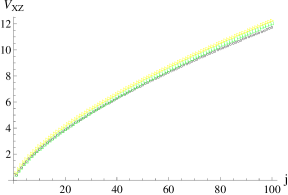
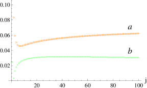
Figure 1: Left: Scaling of the sum of variances $V_{XZ}$ with $j=(1,100)$: (black circles) lower bound of $V_{XZ}$ provided by the ground state energy $\varepsilon_{gs,X}\left(j\right)$ of the Hamiltonian (LABEL:eq:_HTotX); (green squares ) $V_{XZ}^{min_{1}}\left(j\right)$ as in (LABEL:eq:_VXZ_He_scaling); ( yellow triangles) $V_{XZ}^{min_{2}}\left(j\right)$ as in (12). Right: Relative errors obtained with the use of $|\theta_{m}\rangle=\exp\left(-i\theta_{m}H_{TAS}\right)|j,j\rangle$ (see text) as a function of $j=1,..,100$. Curve a (triangles) $|V_{Tot}(|\theta_{m}\rangle)-\varepsilon_{gs,X}|/\varepsilon_{gs,X};$ curve b (circles) $|V_{Tot}(|\theta_{m}\rangle)-V_{XZ}^{min_{1}}\left(j\right)|/V_{XZ}^{min_{1}}\left(j\right)$

The algorithm implemented requires the diagonalization process that eventually determines the value of the bound. However, the structure of the state $|\psi_{sat}\rangle$ able to approximately saturate the bound is not directly apparent from the algorithm unless the ground state is a product state $|\varepsilon_{gs,X}\rangle=|\psi\rangle|\psi\rangle$. In this case, the numerical computations suggest that the ground state is not a in a product form although it provides values which are pretty close to those evaluated in (LABEL:eq:_VXZ_He_scaling). The results obtained can be refined in the following way. For generic $j$ one has that the numerical found ground state energy is doubly degenerate. By fixing $j$ one can explore the ground state manifold in search for a ground state whose Schmidt decomposition can be written as $|\varepsilon_{gs,X}\rangle=\sum_{n}\lambda_{n}|\lambda_{n}\rangle|\lambda_{n}\rangle$ and such that the maximum Schmidt coefficient is sufficiently large. For fixed $j$ we can identify two states $|\lambda_{Max}^{+}\rangle,|\lambda_{Max}^{-}\rangle$ corresponding to two different states $|\varepsilon_{gs,X}^{+}\rangle,|\varepsilon_{gs,X}^{-}\rangle$ both belonging to the ground state manifold and for which the largest Schmidt coefficients coincide. For example with $j=9/2$ one finds sufficiently large values $\lambda_{Max}^{+}=\lambda_{Max}^{-}=0.99619$ . The overlap of the product states with the respective ground states is equal and large i.e., $\left\langle\varepsilon_{gs,+}^{XZ}\right.|\lambda_{Max}^{+}\rangle|\lambda_{Max}^{+}\rangle=\left\langle\varepsilon_{gs,-}^{XZ}\right.|\lambda_{Max}^{-}\rangle|\lambda_{Max}^{-}\rangle=0.996191$. Similar results have be obtained for generic values of $j\leq 100$, thus one one hand both states $|\lambda_{Max}^{+}\rangle,|\lambda_{Max}^{-}\rangle$ constitute good candidates for $|\psi_{sat}\rangle$ and for the (approximate) saturation of the found lower bound, and on the other hand the result is an indirect confirmation that the lower bound provided by $\varepsilon_{gs,X}$ is close to the actual one $l_{B}$.

In order to estimate the error in determining the lower bound via $\varepsilon_{gs,X}$ i.e., $V_{Tot}\left(|\psi_{sat}\rangle\right)-\varepsilon_{gs,X}$, we now proceed with a further refined approach to determine $|\psi_{sat}\rangle$. Indeed, while the states $|\lambda_{Max}^{\pm}\rangle$, which are good candidates for $|\psi_{sat}\rangle$, are obtained numerically it would be desirable to find analogous states that at least in principle can be produced in the laboratory, and that have the same property of $|\lambda_{Max}^{\pm}\rangle$ i.e..to approximately saturate the lower bound. In Appendix D we show how starting from the knowledge of the shape of $|\lambda_{Max}^{\pm}\rangle$ and by means of further physical insights one can indeed identify the following candidate

$$|\theta\rangle = \exp\left(-i\theta H_{TAS}\right)|j,j\rangle$$

where: $|j,j\rangle$ is the eigenstate of $J_{Z}$ corresponding to the eigenvalue $j$; and

$$H_{TAS} = -i\left(J_{+}^{2}-J_{-}^{2}\right)$$

is the two-axis squeezing operator KitagawaSpinSqueezing ; NoriSpinSqueezReview ; the latter having the property of squeezing the state along the $X$ axis and simultaneously anti-squeeze it along the $Y$ axis. As shown in Appendix D, by means of the mapping provided by the Holstein Primakoff approximation, it is possible to infer the optimal value of the squeezing parameter $\theta_{m}=-\frac{\log 2+\log j}{24\ j}$ such that $|\psi_{sat}\rangle=|\theta_{m}\rangle$ provides a good approximation of the lower bound for each $j$. In Figure 1 (right panel, curve b) we plot $|V_{Tot}(|\theta_{m}\rangle)-V_{XZ}^{min_{1}}\left(j\right)|/V_{XZ}^{min_{1}}\left(j\right)$ i.e., the relative error in the evaluation of $V_{Tot}$ with respect to the best bound given by $V_{XZ}^{min_{1}}\left(j\right)$. For $j\leq 100$ the error is firmly below $3\%$, thus showing that the approximation provided by $|\theta_{m}\rangle$ is indeed quite good.
With the aid of $|\theta_{m}\rangle$ we can then provide an estimate of the errors in the determination of the lower bound by means of $\varepsilon_{gs,X}$. In Figure 1 (right panel, curve a) we plot $|V_{Tot}(|\theta_{m}\rangle)-\varepsilon_{gs,X}|/\varepsilon_{gs,X}$; the latter shows that the relative error is for $j\leq 100$ of the order of $6\%$, a result that confirms the goodness of the approximation provided by $\varepsilon_{gs,X}$. Similar results can be obtained directly using $|\lambda_{Max}^{+}\rangle,|\lambda_{Max}^{-}\rangle$ instead of $|\theta_{m}\rangle$.
We finally notice that the state $|\theta_{m}\rangle$ is in principle obtainable in the laboratory via two-axis squeezing and thus is a good candidate for the estimation procedure based on Planar Squeezed states. While the realization of the latter has been proposed in HePQS as the ground state of a two-mode Bose-Einstein condensate and in PQSNDMeasMitchell as the result of a non-demolition quantum measurement protocol, here we provide evidence that the same result can be obtained via two-axis spin-squeezing.

III.3 su(3) operators

We now derive the lower bound for the sum of the variances of $4$ operators belonging to the $su(3)$ algebra. This will allow us to show the results of Proposition 3 in action. Consider the following operators

$$A_{1}=\left(\begin{array}[]{ccc}0&1&0\\ 1&0&i\\ 0&-i&0\end{array}\right), A_{2}=\left(\begin{array}[]{ccc}1&0&0\\ 0&0&0\\ 0&0&-1\end{array}\right)$$

$$A_{3}=\left(\begin{array}[]{ccc}1&1&0\\ 1&0&-1\\ 0&-1&-1\end{array}\right), A_{4}=\left(\begin{array}[]{ccc}1&0&i\\ 0&0&0\\ -i&0&-1\end{array}\right)$$

The bounds for the sum of pair of variances $V_{12}=\Delta^{2}A_{1}+\Delta^{2}A_{2}\geq 15/32$ and $V_{34}=\Delta^{2}A_{3}+\Delta^{2}A_{4}\geq 0.765727$ were found in ZycowskyNumricalRange on the basis of the (uncertainty) numerical range approach. If we compare these results with the approximations $\tilde{l}_{B}^{-}$ obtained within our framework we find that: for $V_{12}$, $\tilde{l}_{B}^{-}=0.4384$ which is approximately $6.5\%$ lower that the value found in ZycowskyNumricalRange ; while for $V_{34}$, $\tilde{l}_{B}^{-}=0.7281$ which is approximately $5\%$ lower that the value found in ZycowskyNumricalRange . As for the lower bound of the sum of the four variances $V_{Tot}=\Delta^{2}A_{1}+\Delta^{2}A_{2}+\Delta^{2}A_{3}+\Delta^{2}A_{4}$ the ground state energy of the corresponding $H_{Tot}$ is different from zero and it provides a first approximation of the searched lower bound i.e., $\varepsilon_{gs}=0.804103$. The problem does not appear to have evident symmetries and in order to check the consistency of $\varepsilon_{gs}$ and to refine the approximation we then use the method outlined in Proposition 3. In Figure (2) we plot the values of the ground states $\varepsilon_{gs,n}^{\alpha}$ of the Hamiltonians $H_{Tot,n}^{\alpha},\ n=1,2,3,4$ as a function of $\alpha\in\left[a_{n1,}a_{n3,}\right]$ i.e., $\alpha$ varying in the interval defined by the lowest/highest eigenvalue of each $A_{n}$. The best lower bound $\tilde{l}_{B}^{-}=\max_{n}\min_{\alpha}\varepsilon_{gs,n}^{\alpha}$is obtained with the Hamiltonian $H_{Tot,1}^{\alpha}$ in correspondence of the value $\alpha=0.963$. The corresponding lower bound $\tilde{l}_{B}^{-}=\varepsilon_{gs,1}^{\alpha=0.963}=1.39932$ is higher than $\varepsilon_{gs}=0.804103$, therefore showing that the method outlined in Proposition 3 allows for a significative refinement of the result. If we now find the Schmidt decomposition of $|\varepsilon_{gs,1}^{\alpha=0.963}\rangle$, we have that the largest Schmidt coefficient is $\lambda_{Max}=0.941487$ and for the corresponding $|\lambda_{Max}\rangle$ the value of $V_{Tot}\left(|\lambda_{Max}\rangle\right)=1.5901$. Therefore the actual bound $l_{B}$ will lie in the interval $\left(\varepsilon_{gs,1}^{\alpha=0.963},V_{Tot}\left(|\lambda_{Max}\rangle\right)\right]=\left(1.39932,1.5901\right]$. Since the Hilbert space has dimension $3$ we have performed a standard minimization procedure directly on $V_{Tot}$ and we have obtained $l_{B}\approx 1.56274$ such that: $\varepsilon_{gs}$ is about half the value $l_{B}$; $\varepsilon_{gs,1}^{\alpha=0.963}$ results to be smaller for about $10\%$; while $V_{Tot}\left(|\lambda_{Max}\rangle\right)$ is just $1.6\%$ higher.

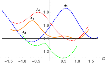
Figure 2: Plot of $\varepsilon_{gs,n}^{\alpha}$ as a function of $\alpha\in\left[a_{n1,}a_{n4,}\right]$ for the operators $A_{1}$ (orange continuous), $A_{2}$ (dash dotted) , $A_{3}$ (dashed) , $A_{4}$ (dotted) . The best lower bound $\varepsilon_{gs,1}^{\alpha=0.963}$ is attained for $H_{Tot,1}^{\alpha=0.963}$ (black continuous horizontal)

III.4 Harmonic oscillator operators $\hat{n},\hat{x}$

While the definition of $H=\sum_{n}H_{n}$ was given for bounded operators, one can use the same definition for unbounded one and use the same mapping (2), which of course remains valid, for finding the relative lower bounds. In the following we show how the procedure and the results of Section II can be applied by focusing a specific example. We consider the operators $\hat{n}$ (number operator) and $\hat{x}$ (position operator) for a single bosonic mode and we seek for the lower bound of

$$V_{xn} = \Delta^{2}\hat{n}+\Delta^{2}\hat{x}$$ (16)

The latter is very much analogous to the bosonic counterpart of $V_{XZ}$ with $j=1$, see equation (D.1) in Appendix D. The analogy with the spin case is strengthened by the three variances sum

$$V_{xpn} = \Delta^{2}\hat{n}+\Delta^{2}\hat{x}+\Delta^{2}\hat{p}\geq 1$$

whose lower bound is again attained by the analog of $|j,j\rangle$ i.e., the vacuum $|0\rangle$ for which $V_{xpn}=1$ and $V_{xn}=1/2$. If one is to reduce $V_{xn}$ one needs to simultaneously reduce $\Delta^{2}\hat{x}<1/2$ and therefore enhance $\Delta^{2}\hat{p}>1/2$.
The starting Hamiltonian here is

$$H_{Tot} = \frac{1}{2}\left(\hat{n}^{2}\otimes\mathbb{I}+\mathbb{I}\otimes\hat{n}^{2}\right)-\hat{n}\otimes\hat{n}+$$

$$+ \frac{1}{2}\left(\hat{x}^{2}\otimes\mathbb{I}+\mathbb{I}\otimes\hat{x}^{2}\right)-\hat{x}\otimes\hat{x}$$

and its approximate ground state energy can be found by expressing $\hat{x}=\left(a+a^{\dagger}\right)/\sqrt{2}$ and by truncating the single mode Fock space i.e., by expressing $H_{Tot}$ in the subspace $\mathcal{H}_{n_{Max}}\otimes\mathcal{H}_{n_{Max}}$ with $\mathcal{H}_{n_{Max}}=span\left\{|0\rangle,|1\rangle,..,|n_{Max}\rangle\right\}$ where $|n\rangle$ is an $n$ bosons state. By letting the maximum number of bosons $n_{Max}$ grow we numerically check that $\varepsilon_{gs}\rightarrow 0$, therefore $H_{Tot}$ itself does not provide a meaningful lower bound. However here we can again resort to the result of Proposition 4 and thus identify the needed modified Hamiltonian. Indeed, the relevant unitary operator here is $U_{\theta}=\exp\left(-i\theta\hat{n}\right)$; one has that $U_{\pi}\hat{x}U_{\pi}^{\dagger}=-\hat{x}$, and the adjoint action of $U_{\pi}\otimes U_{\pi}$ leaves the Hamiltonian $H_{Tot}$ invariant. Therefore, in search for the lower bound we can start restricting ourselves to the states belonging to $S_{\hat{x}}^{0}=\left\{|\psi\rangle\in\mathcal{H}_{bos}|\left\langle\hat{x}\right\rangle=0\right\}$ and consider the Hamiltonian

$$H_{Tot,\hat{x}} = \frac{1}{2}\left(\hat{n}^{2}\otimes\mathbb{I}+\mathbb{I}\otimes\hat{n}^{2}\right)-\hat{n}\otimes\hat{n}+$$

$$+ \frac{1}{2}\left(\hat{x}^{2}\otimes\mathbb{I}+\mathbb{I}\otimes\hat{x}^{2}\right)$$

and its ground state energy $\varepsilon_{gs,\hat{x}}^{0}$ which is a local minimum. For sufficiently high values of $n_{Max}$ one has that $\varepsilon_{gs,\hat{x}}^{0}$ converges to the value $\varepsilon_{gs,\hat{x}}^{0}\approx 0.412721<1/2$. The ground state in this case $|\varepsilon_{gs,\hat{x}}^{0}\rangle\neq|\psi\rangle|\psi\rangle$ is not in a product form, however we can again use the argument outlined in Section II and find the Schmidt decomposition $|\varepsilon_{gs,\hat{x}}^{0}\rangle=\sum_{n}\lambda_{n}|\lambda_{n}\rangle|\lambda_{n}\rangle$. For $n_{Max}=30$ we have that the maximum Schmidt coefficient $\lambda_{Max}\approx 0.99931$ such that one is led to consider the corresponding state $|\lambda_{Max}\rangle|\lambda_{Max}\rangle$ as a fairly good approximation of the ground state. Indeed $\left|\left\langle\varepsilon_{gs,\hat{x}}^{0}\right.|\lambda_{Max}\rangle|\lambda_{Max}\rangle\right|\approx 0.99931$ and therefore $|\psi_{sat}\rangle=|\lambda_{Max}\rangle$ in this case is a good candidate for the minimization of (16). This is confirmed by the value $V_{xn}\left(|\lambda_{Max}\rangle\right)\approx 0.415139$ such that the relative error of the approximation $\left|V_{xn}\left(|\lambda_{Max}\rangle\right)-\varepsilon_{gs,\hat{x}}^{0}\right|/\varepsilon_{gs,\hat{x}}^{0}\approx 0.5\%$ is excellent. While the previous results have been obtained numerically, the following arguments allow one to identify a state realizable in the laboratory that closely approximate $|\lambda_{Max}\rangle$. Just as in the spin case the profile of $|\lambda_{Max}\rangle=\sum_{n=0}^{n_{Max}}\eta_{n}|n\rangle$ is such that only the states with even number of bosons are populated, the distribution of probability is peaked for $n=0$ and it rapidly decreases with $n$. As in the $J_{X},J_{Z}$ case this again hints to the preferred tentative choice of the single mode squeezed state

$$|\xi\rangle = \frac{1}{\sqrt{\cosh\left|\xi\right|}}\sum_{n=0}^{\infty}\left(-\tanh\left|\xi\right|\right)^{n}\frac{\sqrt{\left(2n\right)!}}{2^{n}n!}|2n\rangle$$

as candidate for the minimization of $V_{xn}$. Indeed, in terms of $|\xi\rangle$ (16) reads

$$V_{xn} = 2\sinh^{2}(\left|\xi\right|)\cosh^{2}(\left|\xi\right|)+\frac{\exp\left(-2\left|\xi\right|\right)}{2},$$ (17)

its minimum is obtained for $\xi=\xi_{m}=0.1665679$ and it is equal to $V_{xn}(|\xi_{m}\rangle)=0.41591$ which is a fairly good approximation of $\varepsilon_{gs,\hat{x}}$ and $V_{xn}\left(|\lambda_{Max}\rangle\right)$. Indeed, if one evaluates the fidelity between $|\xi_{m}\rangle$ and the numerically obtained $|\lambda_{Max}\rangle$ one has $\left\langle\xi_{m}\left|\lambda_{Max}\right.\right\rangle=0.999927$; furthermore $\left|\left\langle\varepsilon_{gs,\hat{x}}^{0}\right.|\xi_{m}\rangle|\xi_{m}\rangle\right|=0.999168$ such that $|\xi_{m}\rangle|\xi_{m}\rangle$ also provides a good approximation of the ground state.

Now in principle in order to find whether $\varepsilon_{gs,\hat{x}}^{0}$ is a proper and faithful lower bound one should extend the search to the other sets $S_{\hat{x}}^{\alpha}$, $\alpha\in\left[0,\infty\right]$, which is of course an impossible task. We thus opt for a different strategy. In the first place, the result can be further supported analytically by showing that $|\xi_{m}\rangle$ minimizes $V_{xn}$ over the restricted set of Gaussian states; this is shown in Appendix E. Since the minimum corresponds to $|\xi_{m}\rangle$ with $\left\langle n\right\rangle$ very small, we further support our result by using standard numerical minimization routines and search for the minimum of $V_{xn}$ in a sub space $H_{n_{Max}}=span\left\{|0\rangle,|1\rangle,..,|n_{Max}\rangle\right\}$ with $n_{Max}$ sufficiently large; the numerical results rapidly converge to the lower bound found above.

We have thus shown how the method proposed can in principle work even with sums of variances involving unbounded operators. With the analysis of the Schmidt decomposition of the ground state $|\varepsilon_{gs,\hat{x}}^{0}\rangle$, and the subsequent reasonings and calculations, we have shown that is possible to identify a state that approximately saturates the bound provided by $\varepsilon_{gs,\hat{x}}^{0}$. Therefore even in this case the latter can be considered a good approximation of the actual bound $l_{B}$.

IV Conclusions

In this work we have addressed the problem of finding the state independent lower bound $l_{B}$ of the sum of variances $V_{Tot}\left(|\psi\rangle\right)=\sum_{1}^{N}\Delta_{|\psi\rangle}^{2}A_{n}$ for an arbitrary set $\left\{A_{n}\right\}_{n=1,..,N}$ of Hermitian operators acting on an Hilbert space $\mathcal{H}_{M}$ with dimension $M$. The value $l_{B}$ is the highest positive constant such that $\forall|\psi\rangle\in\mathcal{H_{M}},\ V_{Tot}\left(|\psi\rangle\right)\geq l_{B}$. In general the problem can be solved by finding a sufficiently good approximation $\tilde{l}_{B}^{-}\leq l_{B}$. To this aim we have introduced a method based on a mapping of the minimization problem into the task of finding the ground state energy $\varepsilon_{gs}$ of specific Hamiltonians acting on an extended space $\mathcal{H}_{M}\otimes\mathcal{H}_{M}$. In such way we have shown that $\varepsilon_{gs}=\tilde{l}_{B}^{-}$ i.e., $\varepsilon_{gs}$ provides the required approximation.
In our work we have first provided the main general results that characterize the method proposed and then, by means of different examples, we have described its implementation. While we have shown an instance where $\varepsilon_{gs}=l_{B}$, in general the ground state $|\varepsilon_{gs}\rangle\in\mathcal{H}_{M}\otimes\mathcal{H}_{M}$ corresponding to $\varepsilon_{gs}$ is not in a product form, such that the corresponding $\varepsilon_{gs}=\tilde{l}_{B}^{-}<l_{B}$ will only be an approximation of the actual $l_{B}$, and the bound provided by $\varepsilon_{gs}$ will not be attainable, even though it will still be a valid state independent lower bound. In such cases we have also proposed and tested a method to identify, from the knowledge of the ground state $|\varepsilon_{gs}\rangle\in\mathcal{H}_{M}\otimes\mathcal{H}_{M}$, a state $|\psi_{sat}\rangle\in\mathcal{H}_{M}$ that allows, at least approximately, to saturate the bound i.e., $V_{Tot}\left(|\psi_{sat}\rangle\right)\gtrapprox l_{B}$ . This procedure provides an efficient way to assess the quality of the approximations given by $\varepsilon_{gs}$ and $V_{Tot}\left(|\psi_{sat}\rangle\right)$: the true lower bound $l_{B}$ must lie in the interval $\left(\varepsilon_{gs},V_{Tot}\left(|\psi_{sat}\rangle\right)\right]$. The examples developed show that the latter can be very small, such that even when $\varepsilon_{gs}\neq l_{B}$ the approximations are quite good. While the main general results have been derived for bounded (non-degenerate) operators, we have also shown by means of an example, that the method can be applied to sum of variances involving unbounded operators.
The results presented constitute a first attempt to lay down a general and reliable framework, alternative to the existing ones, for deriving meaningful state independent lower bounds for the sum of variances $V_{Tot}$. As such we have discussed the virtues and limits of the proposed framework. Since the latter is based on ground states evaluation, it does not suffer from the caveats of general minimization schemes that can be numerically demanding and can get trapped in local minima. On the other hand it requires the diagonalization of operators of dimension $M^{2}\times M^{2}$, that for $M$ very large can be numerically complex. As we have shown the complexity of the solution may however be drastically reduced when the problem presents some symmetries and/or the operator involved are simple (e.g. sparse).
While the examples discussed show that the method can indeed be effective, several questions remain open for future research. As we have shown in the paper, since the mapping is not unique, other possibly more effective mappings may be found. The extension of the method to cases involving unbounded operators and the assessment of its limits require a thorough analysis. On another level it would be intriguing to explore the connections, if any, between the framework proposed and the already existing ones e.g. those based on the joint numerical range.
Finally, while in this paper we have not assessed the problem, our method can be used for entanglement detection URHoffmanEntanglementDetection ; URGuneEntanglementDetection and it would be desirable to apply it to relevant problems in that area of research.

Appendix A Properties of $H_{Tot}$

In the following we prove point $ii)$ of Proposition 1 by construction. To this aim we start by supposing that each $A_{n}$ has a non-degenerate eigenspectrum. This hypothesis is in principle not necessary but we use it to simplify the notations. We thus notice that given a state $|\phi\rangle\in\mathcal{H}_{M}\otimes\mathcal{H}_{M}$, since each operator $H_{n}$ is semidefinite positive one has that $\left\langle\phi\left|H_{n}\right|\phi\right\rangle=0$ iff $|\phi\rangle\in Ker\left(H_{n}\right)$. Since we assume that the all $A_{n}$’s have non-degenerate eigenspectrum one has that $\forall n$ $dim\left[Ker\left(H_{n}\right)\right]=M$ each $Ker\left(H_{n}\right)$ can be written as

$$Ker\left(H_{n}\right) = span\left\{|a_{n,1}\rangle|a_{n,1}\rangle,|a_{n,2}\rangle|a_{n,2}\rangle,..\right.$$

$$\left....,|a_{n,M}\rangle|a_{n,M}\rangle\right\}$$

a fact which is easily derived by looking at the form of the generic $H_{n}$ (1): the states $\left\{|a_{n,i}\rangle|a_{n,i}\rangle\right\}_{i=1}^{M}$ are mutually orthogonal, are all eigenstates of $H_{n}$ with zero eigenvalue and they form an orthonormal basis of $Ker\left(H_{n}\right)$. The Hamiltonian $H_{Tot}$ has $\varepsilon_{gs}=0$ iff $\cap_{n}Ker\left(H_{n}\right)\neq\oslash$ such that $|\varepsilon_{gs}\rangle\in\cap_{n}Ker\left(H_{n}\right)$ i.e., iff the intersection of the kernels of the $H_{n}$ operators is not void and the ground state is a common eigenvector of all the $H_{n}$ with zero energy. In order to derive the general form of $|\varepsilon_{gs}\rangle$ we start by supposing that $\cap_{n}Ker\left(H_{n}\right)\neq\oslash$ and that there exist $|\varepsilon_{gs}\rangle\in\cap_{n}Ker\left(H_{n}\right)$. We then focus on on a specific $H_{n}$, say $H_{1}$; since by hypothesis $|\varepsilon_{gs}\rangle\in Ker\left(H_{1}\right)$ we write the state in terms of the eigenbasis (LABEL:eq:_Ker_Hn_eigenbasis) of $Ker\left(H_{1}\right)$

$$|\varepsilon_{gs}\rangle = \sum_{i=1}^{M}\alpha_{1,i}|a_{1,i}\rangle|a_{1,i}\rangle$$

Since $\forall i$ one can write $\alpha_{1,i}=\left|\alpha_{1,i}\right|e^{i\phi_{1,i}}$ and reabsorb the phase factors in the definitions of the eigenvectors, e.g. $|\tilde{a}_{1,i}\rangle=e^{i\phi_{1,i}/2}|a_{1,i}\rangle$ such that

$$|\varepsilon_{gs}\rangle = \sum_{i=1}^{M}\left|\alpha_{1,i}\right||\tilde{a}_{1,i}\rangle|\tilde{a}_{1,i}\rangle$$

In this way the ground state is written in its Schmidt decomposition in terms of the basis $\left\{|\tilde{a}_{1,i}\rangle|\tilde{a}_{1,i}\rangle\right\}_{i=1}^{M}$. Since $|\varepsilon_{gs}\rangle\in\cap_{n}Ker\left(H_{n}\right)$ and due to the structure (LABEL:eq:_Ker_Hn_eigenbasis) of each $Ker\left(H_{n}\right)$, the same is true for all $H_{n}$ such that one has

$$|\varepsilon_{gs}\rangle=\sum_{i=1}^{M}\left|\alpha_{1,i}\right||\tilde{a}_{1,i}\rangle|\tilde{a}_{1,i}\rangle = \sum_{i=1}^{M}\left|\alpha_{2,i}\right||\tilde{a}_{2,i}\rangle|\tilde{a}_{2,i}\rangle=$$

$$= ... =\sum_{i=1}^{M}\left|\alpha_{N,i}\right||\tilde{a}_{N,i}\rangle|\tilde{a}_{N,i}\rangle$$

This result tells us that the ground state must be unique and that $\forall i,n$ it must be $\left|\alpha_{n,i}\right|=1/\sqrt{M}$. Indeed, each decomposition of the ground state (LABEL:eq:_GS_HTot_in_Kernel_basis) represents in principle a different inequivalent versions of the Schmidt decomposition of $|\varepsilon_{gs}\rangle$. But for a pure bipartite state, if the Schmidt coefficients $\left|\alpha_{n,i}\right|$ are not all degenerate i.e., all equal, than the Schmidt decomposition is unique up to phase factors wernerappendix . Since by hypothesis $|\varepsilon_{gs}\rangle\in\cap_{n}Ker\left(H_{n}\right)$, in order for the relation (LABEL:eq:_GS_HTot_in_Kernel_basis) to be true, in the first place it must be $\left|\alpha_{n,i}\right|=1/\sqrt{M},\ \forall n,i$. Therefore if there is a common ground state this must read

$$|\varepsilon_{gs}\rangle=\frac{1}{\sqrt{M}}\sum_{i=1}^{M}|\tilde{a}_{1,i}\rangle|\tilde{a}_{1,i}\rangle = \frac{1}{\sqrt{M}}\sum_{i=1}^{M}|\tilde{a}_{2,i}\rangle|\tilde{a}_{2,i}\rangle=$$

$$= ... =\frac{1}{\sqrt{M}}\sum_{i=1}^{M}|\tilde{a}_{N,i}\rangle|\tilde{a}_{N,i}\rangle$$

Now depending on the problem, there may or may not be the possibility of adjusting the phases $\phi_{i,n}$ in order to have a single ground state with $\varepsilon_{gs}=0$. In the affirmative case the ground state of $H_{Tot}$ is unique and it can be written by using the appropriate phases as $|\varepsilon_{gs}\rangle=\frac{1}{\sqrt{M}}\sum_{i}|\tilde{a}_{n,i}\rangle|\tilde{a}_{n,i}\rangle,\ \forall n$. Form which follows the first part of result $ii)$. It is actually not important for the next part of the result to determine exactly the various $\phi_{i,n}$. Indeed, the non-zero state-independent lower bound $\varepsilon_{1}\left(1-\frac{1}{M}\right)$ can be derived as follows. If $\varepsilon_{gs}=0$, given the general form of the ground state derived above (LABEL:eq:_General_GS_HTot_in_Kernel_basis) i.e., that of a maximally entangled one, for any given $|\phi\rangle\in\mathcal{H}_{M}$ one can write

$$|\varepsilon_{gs}\rangle = \frac{1}{\sqrt{M}}\sum_{i=1}^{M}|a_{n,i}\rangle|a_{n,i}\rangle$$

$$= \frac{1}{\sqrt{M}}\left(\sum_{i=1}^{M}|\phi_{n,i}\rangle|\phi_{n,i}^{*}\rangle\right)$$

where $\left\{|\phi_{n,i}\rangle\right\}_{i=1}^{M}$ being mutually orthonormal and $|\phi\rangle=|\phi_{n,1}\rangle$, while $\forall i\$$|\phi_{n,i}^{*}\rangle$ is the complex conjugate of $|\phi_{n,i}\rangle$ when the latter is expressed in the $\left\{|a_{n,i}\rangle\right\}$ basis. The latest formula allows to infer that $\max_{|\phi\rangle\in\mathcal{H}_{M}}\left|\langle\phi|\langle\phi|\left.\varepsilon_{gs}\right\rangle\right|^{2}=\max_{|\phi\rangle\in\mathcal{H}_{M}}\left|\langle\phi|\left.\phi^{*}\right\rangle\right|^{2}/M=1/M$; the maximum being attained by any state $|\phi\rangle=\sum_{i}U_{ji}|a_{n,i}\rangle$ with $U_{ji}\in\mathbb{R}$. Then, if $\left\{|\varepsilon_{n}\rangle\right\}_{n=0}^{M^{2}-1}$ are the eigenstates of $H_{Tot}$ corresponding to the eigen-energies $\varepsilon_{0}=\varepsilon_{gs}=0$ and $\varepsilon_{n}>0,\ \forall n=1,..,M^{2}-1$, one has that $\forall|\phi\rangle\in\mathcal{H}_{M}$

$$\langle\phi|\langle\phi|H_{Tot}|\phi\rangle|\phi\rangle = \langle\phi|\langle\phi|\sum_{n=0}^{M^{2}-1}\varepsilon_{n}|\varepsilon_{n}\rangle\langle\varepsilon_{n}||\phi\rangle|\phi\rangle=$$

$$\geq \varepsilon_{1}\sum_{n=1}^{M^{2}-1}\left|\langle\phi|\langle\phi|\left.\varepsilon_{n}\right\rangle\right|^{2}=$$

$$= \varepsilon_{1}\langle\phi|\langle\phi|\left(\mathbb{I}_{M^{2}}-|\varepsilon_{gs}\rangle\langle\varepsilon_{gs}|\right)|\phi\rangle|\phi\rangle=$$

$$= \varepsilon_{1}\left(1-\left|\langle\phi|\langle\phi|\left.\varepsilon_{gs}\right\rangle\right|^{2}\right)$$

Since

$$\min_{|\phi\rangle\in\mathcal{H}_{M}}\varepsilon_{1}\left(1-\left|\langle\phi|\langle\phi|\left.\varepsilon_{gs}\right\rangle\right|^{2}\right) = \varepsilon_{1}\left(1-\frac{1}{M}\right)$$

one has that $\forall|\phi\rangle\in\mathcal{H}_{M}$

$$V_{Tot}\left(|\phi\rangle\right)=\langle\phi|\langle\phi|H_{Tot}|\phi\rangle|\phi\rangle \geq \varepsilon_{1}\left(1-\frac{1}{M}\right)>0$$

which is the second part of result $ii)$.

Appendix B Proof of proposition 4

We now prove the results of Proposition 4. We begin with $i)$. Suppose $\alpha>0$, the proof is based on the analysis of the Hamiltonian

$$H_{Tot,n}^{\alpha} = \sum_{m\neq n}H_{m}+\frac{\left(A_{n}^{\alpha}\right)^{2}\otimes\mathbb{I}+\mathbb{I}\otimes\left(A_{n}^{\alpha}\right)^{2}}{2}=$$

$$= H_{Tot,n}-\alpha\left(A_{n}\otimes\mathbb{I}+\mathbb{I}\otimes A_{n}\right)+\alpha^{2}\mathbb{I}$$

where $H_{Tot,n}=\sum_{m\neq n}H_{m}+\frac{A_{n}^{2}\otimes\mathbb{I}+\mathbb{I}\otimes A_{n}^{2}}{2}$ is defined as above. If $|\varepsilon_{gs,n}^{\alpha}\rangle$ is a ground state of $H_{Tot,n}^{\alpha}$ then $|\varepsilon_{gs,n}^{-\alpha}\rangle=U\otimes U|\varepsilon_{gs,n}^{\alpha}\rangle$ must be a ground state of $H_{Tot,n}^{-\alpha}$. Indeed, on one hand, due to the symmetry properies of $\sum_{m\neq n}H_{m}$ that extend to $H_{Tot,n}$, it holds $\langle\varepsilon_{gs,n}^{-\alpha}|H_{Tot,n}|\varepsilon_{gs,n}^{-\alpha}\rangle=\langle\varepsilon_{gs,n}^{\alpha}|H_{Tot,n}|\varepsilon_{gs,n}^{\alpha}\rangle$. Furthermore, due to the action of $U$ on $A_{n}$

$$\langle\varepsilon_{gs,n}^{-\alpha}|\left(A_{n}\otimes\mathbb{I}+\mathbb{I}\otimes A_{n}\right)|\varepsilon_{gs,n}^{-\alpha}\rangle =$$

$$=-\langle\varepsilon_{gs,n}^{\alpha}|\left(A_{n}\otimes\mathbb{I}+\mathbb{I}\otimes A_{n}\right)|\varepsilon_{gs,n}^{\alpha}\rangle$$

such that

$$\varepsilon_{gs,n}^{-\alpha}=\langle\varepsilon_{gs,n}^{-\alpha}|H_{Tot,n}^{-\alpha}|\varepsilon_{gs,n}^{-\alpha}\rangle = \langle\varepsilon_{gs,n}^{\alpha}|H_{Tot,n}^{\alpha}|\varepsilon_{gs,n}^{\alpha}\rangle=\varepsilon_{gs,n}^{\alpha}$$

Then $ii)$ simply follows from the fact that

$$\langle\varepsilon_{gs,n}^{0}|\left(A_{n}\otimes\mathbb{I}+\mathbb{I}\otimes A_{n}\right)|\varepsilon_{gs,n}^{0}\rangle =$$

$$-\langle\varepsilon_{gs,n}^{0}|\left(A_{n}\otimes\mathbb{I}+\mathbb{I}\otimes A_{n}\right)|\varepsilon_{gs,n}^{0}\rangle$$

and there for to first order in $\delta\alpha\ll 1$ one has $\varepsilon_{gs,n}^{\delta\alpha}=\varepsilon_{gs,n}+\delta\alpha^{2}\geq\varepsilon_{gs,n}^{0}$.

Appendix C Symmetries for spin hamiltonian

In this Appendix we detail the symmetries property of $H_{Tot}$ (LABEL:eq:_HTot_JX_JZ) defined in terms of the two spin operators $J_{X},J_{Z}$. One has that

$$e^{-i\theta J_{Y}}J_{Z}e^{i\theta J_{Y}} = \cos\theta J_{Z}+\sin\theta J_{X}$$

$$e^{-i\theta J_{Y}}J_{X}e^{i\theta J_{Y}} = -\sin\theta J_{Z}+\cos\theta J_{X}$$

then, given $U_{YY}=e^{-i\theta J_{Y}}\otimes e^{-i\theta J_{Y}}$

$$U_{YY}J_{Z}\otimes J_{Z}U_{YY}^{\dagger} = \cos^{2}\theta J_{Z}\otimes J_{Z}+\sin^{2}\theta J_{X}\otimes J_{X}+$$

$$+ \sin\theta\cos\theta\left(J_{Z}\otimes J_{X}+J_{X}\otimes J_{Z}\right)$$

$$U_{YY}J_{X}\otimes J_{X}U_{YY}^{\dagger} = \sin^{2}\theta J_{Z}\otimes J_{Z}+\cos^{2}\theta J_{X}\otimes J_{X}+$$

$$- \sin\theta\cos\theta\left(J_{Z}\otimes J_{X}+J_{X}\otimes J_{Z}\right)$$

such that

$$U_{YY}\left(J_{Z}\otimes J_{Z}+J_{X}\otimes J_{X}\right)U_{YY}^{\dagger} = \left(J_{Z}\otimes J_{Z}+J_{X}\otimes J_{X}\right)$$

Furthermore by using the Casimir relation $j(j+1)\mathbb{I=}J_{X}^{2}+J_{Y}^{2}+J_{Z}^{2}$ the Hamiltonian $H_{Tot}$ can be expressed as

$$H_{Tot} = \frac{\left(J_{Z}^{2}+J_{X}^{2}\right)\otimes\mathbb{I}+\mathbb{I}\otimes\left(J_{Z}^{2}+J_{X}^{2}\right)}{2}+$$

$$- \left(J_{Z}\otimes J_{Z}+J_{X}\otimes J_{X}\right)=$$

$$= j(j+1)\mathbb{I}\otimes\mathbb{I}-\frac{J_{Y}^{2}\otimes\mathbb{I}+\mathbb{I}\otimes J_{Y}^{2}}{2}+$$

$$- \left(J_{Z}\otimes J_{Z}+J_{X}\otimes J_{X}\right)$$

such that

$$U_{YY}H_{Tot}U_{YY}^{\dagger} = H_{Tot}$$

therefore $\forall|\phi\rangle\in\mathcal{H}_{M}$ if

$$\langle\phi|\langle\phi|H_{Tot}|\phi\rangle|\phi\rangle = c(\phi)$$

then one has also that

$$\langle\phi|\langle\phi|H_{Tot}|\phi\rangle|\phi\rangle = \langle\phi|\langle\phi|U_{YY}H_{Tot}U_{YY}^{\dagger}|\phi\rangle|\phi\rangle=$$

$$= \langle\phi_{\theta}|\langle\phi_{\theta}|H_{Tot}|\phi_{\theta}\rangle|\phi_{\theta}\rangle$$

$$= c(\phi)$$

Therefore one has a certain degrees of freedom in choosing $|\phi\rangle$ since all states $|\phi_{\theta}\rangle=e^{i\theta J_{Y}}|\phi\rangle,\forall\theta\in\mathbb{R}$ will have the same variance $c(\phi)$ . Now

$$\langle\phi_{\theta}|J_{x}|\phi_{\theta}\rangle = -\sin\theta\langle\phi|J_{z}|\phi\rangle+\cos\theta\langle\phi|J_{x}|\phi\rangle$$

Suppose now $|\phi\rangle$ is a state which minimizes $V_{XZ}$. One can always choose for example $\theta$ such that

$$\langle\phi_{\theta}|J_{x}|\phi_{\theta}\rangle = 0$$

i.e., we can choose $\theta$ by setting

$$\sin\theta\langle\phi|J_{z}|\phi\rangle = +\cos\theta\langle\phi|J_{x}|\phi\rangle$$

$$\tan\theta = \frac{\langle\phi|J_{x}|\phi\rangle}{\langle\phi|J_{z}|\phi\rangle}$$

$$\theta = \arctan\left(\frac{\langle\phi|J_{x}|\phi\rangle}{\langle\phi|J_{z}|\phi\rangle}\right)$$

Therefore even if $\theta$ is unknown we can find the lower bound of $V_{XZ}$ by finding the ground state of the Hamiltonian

$$H_{Tot,X} = \frac{\left(J_{Z}^{2}+J_{X}^{2}\right)\otimes\mathbb{I}+\mathbb{I}\otimes\left(J_{Z}^{2}+J_{X}^{2}\right)}{2}-J_{Z}\otimes J_{Z}$$

Indeed $\varepsilon_{Tot,X}^{0}$ will give a lower bound $\forall|\phi\rangle\in S_{X}^{0}$ among which there will be the $|\phi_{\theta}\rangle$ which minimizes $V_{XZ}$. Then $\forall|\psi\rangle\in\mathcal{H}_{M}$ one has

$$V_{XZ}(|\psi\rangle) \geq V_{XZ}(|\phi_{\theta}\rangle)=$$

$$\geq \varepsilon_{gs,X}^{0}$$

Appendix D Planar spin squeezing

In this Appendix we show how from the knowledge of $|\lambda_{Max}^{+}\rangle,|\lambda_{Max}^{-}\rangle$ one can obtain a state $|\psi_{sat}\rangle=|\theta_{m}\rangle$ that can in principle realized in the laboratory and that approximately saturates the bound for planar spin squeezing. For fixed $j$ one can study the profile of $|\lambda_{Max}^{+}\rangle,|\lambda_{Max}^{-}\rangle$; a feature that holds for all analyzed values of $j$ is that the profile is peaked at $m_{z}=j$ and $m_{z}=-j$ respectively, and such that only the states with $m_{z}=-j+2k$ have non-zero amplitudes. These numerical findings will lead us in the search for states $|\psi_{sat}\rangle$ that on one hand are a good approximations of $|\lambda_{Max}^{+}\rangle,|\lambda_{Max}^{-}\rangle$ and on the other hand are in principle obtainable in the laboratory.
We start by considering the relation (10) which, over the set of eigenstates of $J_{Z}$, is minimized by $|j,\pm j\rangle$ and for such states $\Delta^{2}J_{Z}=0$ and $V_{XZ}=\Delta^{2}J_{X}=j/2$. In order to obtain a lower bound for $V_{XZ}$ smaller than $j/2$, one can imagine to start from the state $|j,j\rangle$ for example and to modify it in such a way that $\Delta^{2}J_{Z}\gtrapprox 0$ is little changed and at the same time $\Delta^{2}J_{X}$ is considerably reduced. This heuristic reasoning suggests the strategy of searching for an operator $G$ such that $|\theta\rangle=\exp\left(-i\theta G\right)|j,j\rangle_{Z}$ $\theta\in\mathbb{R}$ is the state required. If one analyses $V_{XZ}^{\theta}=V_{XZ}(|\theta\rangle)$ and in particular its first order variation $\partial_{\theta}V_{XZ}^{\theta}$ in $\theta=0$ one has

$$\partial_{\theta}\left[\Delta^{2}J_{Z}\left(\theta\right)\right]_{\theta=0} = 0$$

$$\partial_{\theta}\left[\Delta^{2}J_{X}\left(\theta\right)\right]_{\theta=0} = \left\langle j,j\left|\left[J_{X}^{2},G\right]\right|j,j\right\rangle+$$

$$- \left\langle j,j\left|J_{X}\right|j,j\right\rangle\left\langle j,j\left|\left[J_{x},G\right]\right|j,j\right\rangle=$$

$$= 2\ Im\left[\left\langle j,j-2\left|G\right|j,j\right\rangle\right]$$

The previous relations thus leads to consider operators for which $\langle j,j-2|G|j,j\rangle_{z}\neq 0$. The above reasoning heuristically leads to analyze the action of the two-axis squeezing operator

$$H_{TAS} = -i\left(J_{+}^{2}-J_{-}^{2}\right)$$

which is known to have the property of squeezing along the $X$ axis and simultaneously anti-squeezed along the $Y$ axis. This latter property is consistent with the relation (7) where it can be seen that any attempt to squeeze the sum $V_{XZ}$ implies the enhancement of $\Delta^{2}J_{Y}$. The action of the operator $U=\exp\left(-i\theta H_{TAS}\right)$ on $|j,j\rangle$ is not known in an analytical form, however it has the desirable property of populating only the basis states $|j,j-2k\rangle$ thus reproducing one of the features of the states $|\lambda_{Max}^{+}\rangle,|\lambda_{Max}^{-}\rangle$ discussed above.
Following the previous discussion the goal now is to find the optimal value $\theta_{m}$ of the squeezing parameter $\theta$ such that the state $|\psi_{sat}\rangle=|\theta_{m}\rangle=\exp\left(-i\theta_{m}H_{TAS}\right)|j,j\rangle_{Z}$ approximately saturates the lower bound for $V_{XZ}$. This in principle requires for each $j$ the numerical search for the optimal value of $\theta_{m}=\theta_{m}(j)$ for which the minimum of $V_{XZ}^{\theta}$ is attained. We now show how to analytically estimate the optimal value of $\theta_{m}$. As anticipated in the main text we resort to the Holstein-Primakoff (HP) transformation that allows to map the spin operators to harmonic oscillators ones. Indeed as shown in HolsteinPrimakoff ; EmaryDickeHP ; WerAngularMomentum one can write the spin operators in terms of the bosonic creation and annihilation operators $a,a^{\dagger}$.

$$J_{+} = \sqrt{2j}a^{\dagger}\sqrt{1-\frac{a^{\dagger}a}{2j}}$$

$$J_{.-} = \sqrt{2j}\sqrt{1-\frac{a^{\dagger}a}{2j}}a$$

$$J_{z} = a^{\dagger}a-j$$

such that for states with average number of bosons $\left\langle\hat{n}\right\rangle=\left\langle a^{\dagger}a\right\rangle\ll 2j$ one has that $J_{+}=\sqrt{2j}a^{\dagger},\ J_{-}=\sqrt{2j}a$. With this transformation the sum of variances (10) can be written as

$$V_{XZ}^{bos} = \Delta^{2}\hat{n}+j\Delta^{2}\hat{x}$$ (D.1)

where: $\hat{n}$ is the number operator; $\hat{x}=(a+a^{\dagger})/\sqrt{2}$ is the position operator and $\Delta^{2}J_{Z}\rightarrow\Delta^{2}\hat{n}$$\Delta^{2}J_{X}\rightarrow j\Delta^{2}\hat{x}$. Within the Holstein Primakoff representation the spin state $|j,j\rangle$ is mapped into the vacuum $|0\rangle$. In general there is no such mapping between the squeezed state $|\theta\rangle$ and the corresponding single mode squeezed vacuum state that reads ParisGaussianStatesInQInfo

$$|\xi\rangle = \exp\left\{\frac{1}{2}\left[\xi\left(a^{\dagger}\right)^{2}-\xi^{*}a^{2}\right]\right\}|0\rangle$$

with $\xi=re^{-i\phi}$ the squeezing parameter. However, this state is the “natural” counterpart of $|\theta\rangle$ in the search for a minimum of $V_{XZ}^{bos}$ . Within the HP framework two-axis squeezing operator transforms into the single-mode squeezing operator

$$e^{-i\theta H_{TAS}} = \exp\left[-\theta\left(J_{+}^{2}-J_{-}^{2}\right)\right]=$$

$$\approx \exp\left\{-\theta 2j\left[\left(a^{\dagger}\right)^{2}-a^{2}\right]\right\}$$

such that if we now choose $\xi=-4j\theta$ we can bridge the spin and the bosonic version of $V_{XZ}$. With these assumptions $V_{XZ}^{bos}$ reads

$$V_{XZ}^{boson}\left(\theta\right) = 2\sinh^{2}(4j\theta)\cosh^{2}(4j\theta)+j\frac{\exp\left(8j\theta\right)}{2}$$

The minimization of the latter expression with respect to $\theta$ provides a single real solution that for $j\gg 1$ can be written as

$$\theta_{m} = -\frac{\log 2+\log j}{24\ j}+o\left(1/j^{2}\right)$$ (D.3)

such that for $j\gg 1$ one finds

$$V_{XZ}^{boson}\left(\theta_{m}\right) \approx 0.595275\ j^{2/3}$$

We notice that the scaling obtained in the HP framework coincides with the dominant part of (LABEL:eq:_VXZ_He_scaling) for large $j$. The found approximate solution $\theta_{m}$ can now be used to compute the bound for the spin version of the sum of variances (10) i.e., $V_{XZ}(|\theta_{m}\rangle)$. The consequences of this results are described in the Main text.

Appendix E The bosonic case: gaussian states

The generic pure Gaussian state reads

$$D(\alpha)S(\xi)|0\rangle = |\alpha,\xi\rangle$$

The variance of $x$ for such states can thus be written as

$$\Delta_{|\alpha,\xi\rangle}^{2}x = \left\langle\alpha,\xi\left|x^{2}\right|\alpha,\xi\right\rangle-\left\langle\alpha,\xi\left|x\right|\alpha,\xi\right\rangle^{2}=$$

$$= \left\langle\xi\left|D^{\dagger}(\alpha)xD(\alpha)D^{\dagger}(\alpha)xD(\alpha)\right|\xi\right\rangle+$$

$$- \left\langle\xi\left|D^{\dagger}(\alpha)xD(\alpha)\right|\xi\right\rangle^{2}=$$

$$= \Delta_{|\xi\rangle}^{2}x_{\alpha}$$

with $x_{\alpha}=D^{\dagger}(\alpha)xD(\alpha)=x+2Re\left[\alpha\right]\mathbb{I}$. Since $\Delta^{2}\left[A+c\mathbb{I}\right]=\Delta^{2}A$ one has that $\Delta_{|\alpha,\xi\rangle}^{2}\hat{x}=\Delta_{|\xi\rangle}^{2}\hat{x}$. i.e., the displacement does not change the variance of $x$, since it only changes its average value. We now evaluate the variance of $\hat{n}$ and find $\Delta_{|\alpha,\xi\rangle}^{2}\hat{n}=\Delta_{|\xi\rangle}^{2}\hat{n}_{\alpha}$ with $n_{\alpha}=n+a^{\dagger}\alpha+a\alpha^{*}+\left|\alpha\right|^{2}$. The constant $\left|\alpha\right|^{2}$ again can be dropped and one is left with such that

$$\Delta_{|\xi\rangle}^{2}\hat{n}_{\alpha} = \Delta_{|\xi\rangle}^{2}\hat{n}+2\left|\alpha\right|^{2}\Delta_{|\xi\rangle}^{2}\hat{x}_{\arg\alpha}+$$

$$+ \left|\alpha\right|\left[\left\langle\hat{n}\hat{x}_{\arg\alpha}\right\rangle+\left\langle\hat{x}_{\arg\alpha}\hat{n}\right\rangle-2\left\langle\hat{n}\right\rangle\left\langle\hat{x}_{\arg\alpha}\right\rangle\right]$$

where $\hat{x}_{\arg\alpha}=(ae^{i\ \arg\alpha}+a^{\dagger}e^{-i\ \arg\alpha})/\sqrt{2}$. Since the averages are taken for the state $|\xi\rangle$, for the property of the latter one has $\left\langle\hat{n}\hat{x}_{\arg\alpha}\right\rangle=\left\langle\hat{x}_{\arg\alpha}\hat{n}\right\rangle=\left\langle\hat{x}_{\arg\alpha}\right\rangle=0$. Overall the previous results show that, $\forall\alpha,\xi$ i.e., for all pure Gaussian states $|\alpha,\xi\rangle$

$$\Delta_{|\alpha,\xi\rangle}^{2}n+\Delta_{|\alpha,\xi\rangle}^{2}x = \Delta_{|\xi\rangle}^{2}n+2\left|\alpha\right|^{2}\Delta_{|\xi\rangle}^{2}x_{\arg\alpha}+\Delta_{|\xi\rangle}^{2}x\geq$$

$$\geq \Delta_{|\xi\rangle}^{2}n+\Delta_{|\xi\rangle}^{2}x$$

such that the minimum of $V_{xn}$ over the set of Gaussian state is given by the squeezed vacuum state $|\xi_{m}\rangle$ that minimizes $\Delta_{|\xi\rangle}^{2}n+\Delta_{|\xi\rangle}^{2}x$.