Numerical models for evolution of extreme wave groups

Abstract

The paper considers the application of two numerical models to simulate the evolution of steep breaking waves. The first one is a Lagrangian wave model based on equations of motion of an inviscid fluid in Lagrangian coordinates. A method for treating spilling breaking is introduced and includes dissipative suppression of the breaker and correction of crest shape to improve the post breaking behaviour. The model is used to create a Lagrangian numerical wave tank, to reproduce experimental results of wave group evolution. The same set of experiments is modelled using a novel VoF numerical wave tank created using OpenFOAM. Lagrangian numerical results are validated against experiments and VoF computations and good agreement is demonstrated. Differences are observed only for a small region around the breaking crest.

Keywords— Lagrangian wave modelling, OpenFOAM, wave groups, breaking waves

1 Introduction

Theoretical analysis and field evidence show that the largest waves belong to wave groups. From the analysis of Gaussian random processes [1], it follows that, in the linear approximation, the average profile of an extreme wave in a random Gaussian sea is a wave group, whose shape is proportional to the autocorrelation function of the random process. The theoretical results are confirmed by field measurements [2, 3]. Focussed wave groups were suggested as design waves [4] and are often used in computations of wave structure interaction [5, 6].

The evolution of steep travelling wave groups includes complex physical processes occurring over a wide range of time and space scales, e. g. long-term nonlinear wave evolution and wave breaking. A numerical model capable of adequately describing such processes should meet a wide range of sometimes conflicting requirements. Advantages and disadvantages of different numerical models make them suitable for modelling different aspects of the wave group evolution. It is therefore natural to combine different models to model different stages of wave evolution. This leads to the development of so-called coupled or hybrid models. In hybrid models, a relatively simple and computationally efficient model is used to simulate the long-term evolution of a steep wave up until the initial development of the overturning crest. Results of these calculations are then used as initial conditions for a model capable to resolve the interaction of the overturning crest with the underlying water surface. Similarly, for wave-structure interaction problems the far-field wave evolution can be modelled by a fast model and the region near the structure by a more sophisticated but computationally expensive model. This approach has now received considerable attention and numerous hybrid models have been developed. The most popular hybrid models usually couple a Boundary Element Method (BEM) model for the far-field calculations and a Volume of Fluid (VoF) model for the wave-structure interaction [7, 8]. Further examples include the coupling of a Boussinesq model with an Smooth Particle Hydrodynamics (SPH) model [9] and BEM with SPH [10]. A brief literature review on the subject of models coupling can be found in [8].

An alternative method to describe water waves is using equations of fluid motion in Lagrangian formulation. These equations are written in material coordinates moving together with the fluid. Each material point of fluid continuum is marked by a specific label, and the labels create a continuous set of Lagrangian coordinates. In the Lagrangian description the free surface is represented by a fixed boundary of the domain in Lagrangian coordinates and equations of fluid motion in Lagrangian form to be solved in a fixed domain of Lagrangian labels. Some numerical methods utilise certain elements of the Lagrangian description. For example, in boundary element methods time integration is often based on a mixed Eulerian-Lagrangian (MEL) formulation, which traces fluid particles on the free surface [11, 12]. The SPH approach can be considered as fully Lagrangian. In this method, the fluid domain is represented by a set of material particles, which serve as physical carriers of fluid properties. An integral operator with a compact smoothing kernel is used to represent average properties of fluid at a certain location. Each particle interacts with nearby particles from a domain specified by the smoothing kernel [13, 14]. However, SPH models do not refer to equations of fluid motion in Lagrangian coordinates and therefore differ from methods in which the Lagrangian equations are directly applied to solve water wave problems.

The first works using equations of fluid motion in Lagrangian formulation with applications to water wave problems appeared in early 70’s. The formulation included kinematic equations of mass and vorticity conservation for internal points of a domain occupied by an ideal fluid [15]. The dynamics of the flow was determined by a free-surface dynamic condition. An alternative approach used Navier-Stokes equations in material coordinates moving together with fluid [16]. The next step was the development of an Arbitrary Lagrangian-Eulerian (ALE) formulation [17]. ALE uses a computational mesh moving arbitrarily within a computational domain to optimise shapes of computational elements and a problem is formulated in moving coordinates connected to the mesh. For example, Eulerian (fixed mesh) or fully Lagrangian (fluid moving mesh) formulations can be used in different areas. Implementation of a finite element approach with irregular triangular meshes for ALE formulation [18] led to the development of a sophisticated method capable of solving complicated problems with interfaces [19]. However, ALE models are complicated both in terms of formulation and numerical realisation and lack the main advantage expected of a Lagrangian method, namely the simplicity of representing computation domains with moving boundaries. The deformation of elementary fluid volumes remains comparatively simple for many problems solved within the ideal fluid framework. Such problems include the evolution of propagating wave groups and can be efficiently treated with much simpler Lagrangian models, like the model described in [15].

The current work focuses on the development of a new version of a fully Lagrangian finite-difference model, which has been previously applied to simulate tsunami waves in a wave flume [20], violent sloshing in a moving tank [21] and the propagation of wave groups on sheared currents [22, 23]. The original Lagrangian model is modified to include a dispersion correction term, which increases the order of approximation of the dispersion relation and considerably reduces long-term dispersion errors. To continue the calculations through the wave breaking, we implement breaking suppression by local surface damping. It turns out, that elimination of the crest overturning leads to errors in the wave shape after the breaking. To reduce this error, we implement a procedure for crest shape correction. The model demonstrates certain advantages over alternative methods for modelling water waves, like Boundary Element Methods. In particular, BEM methods use potential formulation and can not be used for rotational flows. The Lagrangian model can be applied to flows with arbitrary distribution of vorticity, which allows its application to problems with sheared currents [22, 23]. This feature is also useful for the accurate simulation of post breaking wave evolution since wave breaking results in intense vortical motion. At the same time, the new Lagrangian model remains relatively simple and can thus be optimised for high computational efficiency.

The new version of the Lagrangian model can be considered as a good candidate for the fast element of a hybrid model. For a hybrid model it is important that model elements generate consistent results for surface elevation and kinematics at the vicinity of high crests, when switching between the two models takes place. To demonstrate the compatibility of models, we perform a detailed comparison of surface elevation and kinematics between the Lagrangian model and a VoF model, which is a typical candidate for a second component of a hybrid model. We use an open source realisation of a VoF method implemented in olaFlow, which is a numerical two-phase flow solver with a core based on OpenFOAM. The model includes a module for moving-boundary wave generation and absorption [24, 25]. This extension allows simulation of piston and flap type wave makers and, therefore, direct comparison between results generated in different numerical models and in experiments using identical wave generation methods. First, we validate both models against experimental measurements of surface elevation of wave groups in a wave tank. Numerical wave tanks (NWT) replicating the experimental set-up are created in each model and the displacement of the experimental wavemaker is used as input for both NWTs. This allows direct comparison between numerical and experimental results and between the models. After validation, the Lagrangian model and olaFlow are applied to simulate the evolution of a steep breaking wave group. The surface elevation and flow kinematics computed with the Lagrangian model and olaFlow are then compared. Particular attention is paid to the surface elevation before, during and after the breaking onset and to the flow kinematics under the high nearly breaking crest.

2 Experimental data

Numerical results presented in this paper are validated against a set of experimental data on the propagation of focussed wave groups obtained in the wave flume of the Civil Engineering department at UCL. The flume is $45\,$cm wide with a $12.5$ m long working section extending between two piston-type wavemakers. The wavemaker on the right end of the flume generates waves, while the opposite paddle acts as a wave absorber. For all tests, the water depth over a horizontal bed of the flume was set at $h=40$ cm. The centre of the flume is used as the origin of the coordinate system with the $x$-axis directed towards the wave generator positioned at $x=6.25$ m. The vertical $z$-axis originates from the still water surface and is directed upwards. The wavemaker is controlled by a force feedback system, which operates in the frequency domain. Input of the control system is the linearised amplitude spectrum of the generated wave. The control system uses discrete spectra and generates periodic paddle motions. For our experiments we use an overall return period of $64\,$sec, which is the time between repeating identical events produced by the paddle. The range of frequencies used by the wave generator is from $1/64$ to $2\,$Hz with $128$ equally-spaced discrete frequency components $f_{n}=n/64$ Hz; $n=1\dots 128$. Overall, the system allows precise control of wave generation and provides partial absorption of the incoming waves at the further end of the flume. The surface elevation is monitored with a series of six resistance wave probes and an ultrasonic sensor is used to record the paddle motion. A schematic of the experimental layout can be seen in Figure 1.

Figure 1: Wave flume layout and positions of wave probes.

The wavemaker control does not account for dissipative and nonlinear effects, and the spectrum of a generated wave group differs from the input spectrum of the control system. The iterative procedure described in [26] is used to produce waves with the desired spectrum and focussed at the centre of the flume. We apply the iterations to generate a Gaussian wave group with peak frequency of $f_{p}=1$ Hz focussed at the centre of the flume with the linear focus amplitude of $2.5\,$cm. Then we use the resulting input spectrum to generate higher amplitude waves by multiplying the input by factors of 2 and 3 without further corrections to phase or amplitude. We therefore obtain waves with linear focus amplitudes $A=5\,$cm and $A=7.5\,$cm. For all cases waves with constant phase shifts $\Delta\phi=\pi/2$, $\pi$ and $3\pi/2$ were also generated. For example, the phase shift $\Delta\phi=\pi$ corresponds to the wavemaker input opposite to the original wave. Wave records with shifted phases can be used for their spectral decomposition and linearisation [26]. The linearised spectra of generated waves at $x=0$ are shown on Figure 2. As expected, nonlinear defocussing and transformation of the spectrum can be observed for higher amplitude waves. The resulting waves are of tree distinct qualitative types. The small amplitude waves ($A=2.5\,$cm) have weakly nonlinear features. The waves with $A=5\,$cm can be described as strongly nonlinear non-breaking waves. And the high amplitude waves ($A=7.5\,$cm) exhibits intense breaking events as they travel along the flume.

Six return periods are generated in each experimental run. The first period initiates from still water conditions and thus the surface elevation record differs from the records for the following five return periods. The records for these five periods demonstrate a high level of repeatability. It was therefore assumed that the periodic wave system with the return period of $64$ sec is established in the flume after the first period. The data for the first return period are neglected and the rest of the data are averaged between the following five periods. This reduces contributions from all components with periods other than the return period, including high frequency noise and sloshing modes of the flume. Each of the six-period runs was repeated at least three times, demonstrating a high level of repeatability.

Figure 2: Linearised spectra of experimental wave groups at a focus point. Amplitude (left) and phase (right). Solid– $A=2.5$ cm; dashed– $A=5\,$cm; dash-dotted– $A=7.5\,$cm.

3 Lagrangian numerical model

3.1 Mathematical and numerical formulation

A general Lagrangian formulation for two-dimensional flow of inviscid fluid with a free surface can be found in [27]. We consider time evolution of coordinates of fluid particles $x(a,c,t)$ and $z(a,c,t)$ as functions of Lagrangian labels $(a,c)$. The formulation includes the Lagrangian continuity equation and the Lagrangian form of vorticity conservation

$$\frac{\partial(x,z)}{\partial(a,c)}=J(a,c)\,;\quad\frac{\partial(x_{t},x)}{\partial(a,c)}+\frac{\partial(z_{t},z)}{\partial(a,c)}=\Omega(a,c)\,,$$ (1)

and the dynamic free-surface condition

$$x_{tt}x_{a}+z_{tt}z_{a}+g\,z_{a}\,\big{|}_{c=0}=0\,.$$ (2)

Functions $J(a,c)$ and $\Omega(a,c)$ are given functions of Lagrangian coordinates and should be provided as a part of the problem formulation.

For the convenience of the numerical realisation, we modify the original equations (1) and write them in the following form

$$\Delta_{t}\left(\frac{\partial(x,z)}{\partial(a,c)}\right)=0;\qquad\Delta_{t}\left(\frac{\partial(x_{t},x)}{\partial(a,c)}+\frac{\partial(z_{t},z)}{\partial(a,c)}\right)=0\,,$$ (3)

where the operator $\Delta_{t}$ denotes the change between time steps. From the point of view of the numerical realisation, equations (3) mean that values in brackets at two time steps are equal to one another. This formulation does not require explicit specification of functions $J(a,c)$ and $\Omega(a,c)$, which are specified implicitly by the initial conditions. $J(a,c)$ is defined by initial positions of fluid particles associated with labels $(a,c)$ and $\Omega(a,c)$ is the vorticity distribution, which is defined by the velocity field at the initial time. We also modify the dynamic free surface condition (2) by adding various service and physical terms to the right-hand side

$$x_{tt}x_{a}+z_{tt}z_{a}+g\,z_{a}={-RHS(a,t)}\,\Big{|}_{c=0}\,.$$ (4)

We use the following set of additional terms

$$RHS(a,t)={k\,(x_{t}\,x_{a}+z_{t}z_{a})}\,+\,{\sigma\,\frac{\partial}{\partial\,a}\,\frac{\partial\,\kappa}{\partial\,t}}\,+\,{\gamma\,\frac{\partial\kappa}{\partial a}}\,,$$ (5)

where $\kappa$ is the surface curvature. The first term in (5) introduces damping of displacement of surface particles with the damping coefficient $k(a)$. This term is used for absorbing reflections from a boundary of a numerical wave tank opposite to a wavemaker. The second term represents damping of surface curvature and $\sigma(a)$ is the corresponding damping coefficient. As described later in this paper, it is used to simulate the dissipative effects of wave breaking. The third term represents surface tension with the coefficient $\gamma$.

A specific problem within the general formulation is defined by boundary and initial conditions. In this paper boundary conditions are used to simulate the experimental wave tank presented on Figure 1. We use a rectangular Lagrangian domain with $c=0$ being the free surface and $c=-h$ being the bottom. The known shape of the bottom provides the condition on the lower boundary of the Lagrangian domain. For the case of a flat bed of depth $h$ we have $z(x,-h)=-h$. On the right boundary of the Lagrangian domain $a=a_{\max}$ a moving vertical wall represents a piston wavemaker:

$$x(a_{\max},c,t)=a_{\max}+X_{\mathrm{wm}}(t)\,,$$ (6)

where $X_{\mathrm{wm}}(t)$ is the prescribed wavemaker motion. A solid vertical wall is used on the left boundary $x(a_{\min})=a_{\min}$. An absorption region is implemented to reduce reflections from the wall. Still water initial conditions are used to specify initial velocities and positions of fluid particles. The set of equations (3) with the free surface boundary condition (4, 5) and the conditions on the tank boundaries is solved numerically using a finite-difference technique.

Since equations (3) for internal points of a computational domain include only first order spatial derivatives, a compact four-point Keller box scheme [28] can be used for finite-difference approximation of these equations. For our selection of the Lagrangian domain the stencil box can be chosen with sides parallel to the axes of the Lagrangian coordinates, which significantly simplifies the final numerical scheme. The values of the unknown functions $x$ and $z$ on the sides of the stencil box are calculated as averages of values at adjacent points and then used to approximate the derivatives across the box by first-order differences. The scheme provides the second-order approximation for the box central point. Time derivatives in the second equation in (3) are approximated by second-order backward differences. Spatial derivatives in the free-surface boundary condition are approximated by second-order central differences and second-order backward differences are used to approximate time derivatives. As demonstrated below, this leads to a numerical scheme with weak dissipation. The overall numerical scheme is of the second order in both time and space.

A fully-implicit time marching is applied, and Newton method is used on each time step to solve the nonlinear algebraic difference equations. The scheme uses only 4 mesh points in the corners of the box for internal points of the fluid domain. Therefore, the resulting Jacobi matrix used by nonlinear Newton iterations has a sparse 4-diagonal structure and can be effectively inverted using algorithms, which are faster and less demanding for computational memory than general algorithms of matrix inversion. The current version of the solver uses a standard routine for inversion of general sparse matrices [29]. To reduce calculation time, the inversion of a Jacobi matrix is performed at a first step of Newton iterations and if iterations start to diverge. Otherwise, a previously calculated inverse Jacobi matrix is used. Usually only one matrix inversion per time step is required. To start time marching, positions of fluid particles at three initial time steps should be provided, which specifies initial conditions for both particle positions and velocities. An adaptive mesh is used in the horizontal direction with an algorithm based on the shape of the free surface in Lagrangian coordinates $z(a,0,t)$ to refine the mesh in regions of high surface gradients and curvatures. Constant mesh refinement near the free surface is used in the vertical direction.

Since the finite-difference approximation presented above uses quadrangular mesh cells, it may be subjected to the so called alternating errors caused by non-physical deformations of cells [16, 17]. This deformation preserves the overall volume (area) of a cell, as prescribed by finite difference approximation of the Lagrangian continuity equation. However, volumes of triangles build on cell vertexes can change. The area of one of the triangles increases while the area of the second triangle decreases by the same value. This leads to alternating distortions of neighbouring cells, resulting in instability of short-wave disturbances with a wavelength equal to two cell spacing. It is usual to implement artificial smoothing to suppress this instability [17]. For the presented model, efficient suppression of the instability caused by alternating errors is provided by an adaptive mesh. After several time steps the solution is transferred to a new mesh using quadratic interpolation. The effect of this procedure is similar to regridding used in [30]. It reduces short-wave disturbances and does not produce unwanted damping. Alternating errors remain the main reason for calculations breakdown. However, this happens for large deformations of the domain associated, for example, with wave breaking. Otherwise, the numerical scheme is stable with respect to this type of instability

3.2 Numerical dispersion and dispersion correction

For travelling waves dispersion errors can be the main source of numerical errors. Therefore, special attention must be paid to approximation of the dispersion relation. To derive the numerical dispersion relation we use the continuous representation of the finite difference scheme. In this method the finite difference operators are expanded to Taylor series with respect to small discretisation steps. For example, a 3-point backward difference approximation of the second time derivative can be expressed as

$$\begin{split}\frac{-f(t-3\,\tau)+4\,f(t-2\,\tau)-5\,f(t-\tau)+2\,f(t)}{\tau^{2}}=\qquad\qquad\qquad\\ =f^{\prime\prime}(t)-\frac{11}{12}\,\tau^{2}\,f^{\prime\prime\prime\prime}(t)+O(\tau^{3})\,.\end{split}$$ (7)

As can be seen, the approximation is of the second order with the leading term of the error proportional to the fourth derivative of a function, which gives the main contribution to the error. Similar continuous representations can be derived for all other difference operators.

We consider the spatial and temporal discretisation according to the numerical scheme described above with the time step $\tau$ and spatial steps $(\delta a;\delta c)$. Under an assumption of small perturbations of the original particle positions, we represent unknown functions in the form

$$x=a+\varepsilon\,\xi(a,c,t);\quad z=c+\varepsilon\,\zeta(a,c,t)$$

and keep only linear terms of expansions with respect to the small displacement amplitude $\varepsilon\to 0$. The unknown functions $\xi$ and $\zeta$ represent displacements of fluid particles from the original positions. The solution for a regular travelling wave in deep water can be written as

$$\xi=i\,e^{i\,k\,a}\,e^{\varkappa\,c}\,e^{i\,\omega\,t}\,;\quad\zeta=e^{i\,k\,a}\,e^{\varkappa\,c}\,e^{i\,\omega\,t}\,.$$

Because of the discretisation error, the constant for the exponential decay of the displacement with the depth $\varkappa$ is not equal to the wavenumber $k$. We are looking for the solutions for $\omega$ and $\varkappa$ as expansions with respect to small discretisation parameters. The expansion for $\varkappa$ should satisfy the discrete version of (1). The expansion for $\omega$ defines the numerical dispersion relation and is used to satisfy the free-surface condition (2). The corresponding expansions are found to be

$$\varkappa/k=1-\frac{1}{24}\,(\,\delta\hat{a}^{2}+\delta\hat{c}^{2}\,)+O(\delta\hat{a}^{4};\delta\hat{c}^{4})$$ (8)

and

$$\omega/\sqrt{gk}=\,\pm 1\mp\frac{1}{24}\,(11\,\hat{\tau}^{2}+2\,\delta\hat{a}^{2})+\frac{1}{2}\,i\,\hat{\tau}^{3}+O(\hat{\tau}^{4};\delta\hat{a}^{4})\,,$$ (9)

where the nondimensional discretisation steps $\hat{\tau}=\sqrt{gk}\,\tau$, $\delta\hat{a}=k\,\delta a$ and $\delta\hat{c}=k\,\delta c$ are used. As can be seen, the numerical dispersion relation (9) incorporates a numerical error to dispersion at the second order and has a weak dissipation at the third order. Equation (8) shows that there is also a second-order error in the displacement of fluid particles. It is interesting to note that the dispersive error is affected only by the horizontal discretisation step, while the vertical discretisation affects the kinematics of fluid particles under the surface. Therefore, if we are interested in the evolution of the waveform, we can use relatively few vertical mesh points.

Validation tests show that the achieved convergence rate for the second-order dispersion approximation is not sufficient. To increase the approximation order for the dispersion relation we introduce dispersion correction terms to the free surface boundary condition. These terms should satisfy the following conditions: (i) to have the order of $O(\tau^{2};\delta a^{2})$; (ii) to be linear; (iii) not include high derivatives; (iv) to use the same stencil as the original scheme and (v) to reduce the order of the dispersion error. It has been found that the free surface boundary condition (2) with the dispersion correction term satisfying these conditions can be written as follows

$$x_{tt}x_{a}+z_{tt}z_{a}+g\,z_{a}+\left(\frac{1}{6}\delta a^{2}\,x_{aa,tt}-\frac{11}{12}g\,\tau^{2}z_{a,tt}\right)=0\,\Big{|}_{c=0}\,,$$ (10)

where the dispersion correction term is given in brackets. The term $x_{aa}$ with the second-order spatial derivative leads to high-wavenumber nonlinear instability for large wave amplitudes. To suppress this instability, we apply 5-point quadratic smoothing to function $x$ at the surface before applying the finite-difference operator. The smoothing is applied only to this term in (10). It is applied at the future time layer to ensure that the scheme remains fully implicit. It can be shown that the numerical dispersion relation becomes

$$\omega/\sqrt{gk}=\,\pm 1+\frac{1}{2}\,i\,\hat{\tau}^{3}\pm\,(\frac{361}{480}\hat{\tau}^{4}-\frac{1}{360}\delta\hat{a}^{4})-\frac{13}{12}\,i\,\hat{\tau}^{5}+O(\hat{\tau}^{6};\delta\hat{a}^{6})\,.$$ (11)

We now have weak numerical dissipation at 3-rd order and the dispersion error at 4-th order. A term with weak negative dissipation at 5-th order should also be noted. This term can potentially lead to solution instability for large time steps.

3.3 Treatment of breaking

$N_{x}$	$N_{z}$			$\delta t$, sec	$N_{x}$	$N_{z}$			$\delta t$, sec
101	11	16	21	0.010	251	11	16	21	0.004
126	11	16	21	0.008	401	11	16		0.0025
201	11	16	21	0.005	501	11			0.002

Table 1: Numerical cases for convergence and validation tests of the Lagrangian model.

A disadvantage of the Lagrangian model, BEM models and other simple models of wave propagation is their inability to model spilling breaking. Temporal and spatial scales of evolution of a breaking crest are small compare to a typical wave period, wave length and wave amplitude. This leads to a singularity in a numerical solution, which causes breakdown of computations. The Lagrangian model can simulate overturning waves and therefore with sufficient spatial and temporal resolution it can resolve micro-plungers originating at wave crests during the initial stages of spilling breaking. However, the model can not continue calculations after the self-contact of the free surface has occurred and the solution becomes nonphysical. This makes it impossible to apply the model to steep progressive waves and extreme sea conditions. Removing a singularity in the vicinity of the breaking crest can help continuing calculations with only a minor effect on the overall wave behaviour. This can be achieved by implementing artificial local dissipation in the vicinity of a wave crest prior to breaking. With this approach all small-scale local features would disappear from the solution, but the overall behaviour of the wave would be represented with good accuracy. Practical implementation of the method employs a breaking criterion to initiate dissipation right before breaking occurs. The dissipation is usually enforced by including damping terms in the free-surface boundary conditions [31, 32]. Recently, a breaking model based on an advanced breaking criterion and an eddy viscosity dissipation model was implemented in a spectral model of wave evolution [33, 34]. The method demonstrates a good comparison with the experiments and allows to apply spectral models to simulate evolution of severe sea states with breaking.

In this paper we use a method of treatment for spilling breaking, which uses the same basic concept but differs in its details of realisation. The method includes dissipative suppression of the breaker and correction of crest shape to provide accurate post-breaking behaviour of the wave. There are several conditions such a method should satisfy: (i) to act locally in the close vicinity of a developing singularity without affecting the rest of the flow; (ii) to simulate energy dissipation caused by breaking; (iii) to be mesh-independent, that is the change of the effect with changing mesh resolution should be within the accuracy of the overall numerical approximation and (iv) to be naturally included into a problem formulation representing an actual or artificial physical phenomenon. The development of a spilling breaker is associated with a rapid growth of surface curvature. Therefore, the local dissipation effect satisfying these conditions can be created by adding a term $-\sigma\,\partial/\partial a\,(\,\partial\kappa/\partial t\,)$ to the right hand side of the free surface dynamic condition (4, 5). This term with a small coefficient $\sigma$ introduces artificial dissipation due to the change of surface curvature $\kappa$, which acts locally at the region of fast curvature changes and suppresses breaker development without affecting the rest of the wave. To minimise the undesirable effect of dissipation, the action of the damping term is limited both in time and in space. Breaking dissipation is triggered when the maximal acceleration of fluid particles at the crest exceeds a specified threshold $a_{\mathrm{on}}$ and it goes off when the maximum acceleration falls below a second lower value $a_{\mathrm{off}}$. The appropriate values for activation and deactivation thresholds are $a_{\mathrm{on}}=g$ and $a_{\mathrm{off}}=0.5\,g$. Spatially, the action of the breaking model is limited by the half-wavelength between the ascending and descending crossing points around a breaking wave crest.

Figure 3: $L_{2}$-norm of difference between amplitude (left) and phase (right) spectra of a wave group at $x=0$ measured in experiment and calculated by the Lagrangian solver. Top – $A=5$ cm; without (solid) and with (dashed) dispersion correction. Bottom – $A=7.5$ cm; breaking control without (solid) and with (dashed) crest correction. $N_{z}=11$.

Activation of the damping term makes it possible to continue the calculation beyond the breaking event. However, the resulting shape of the wave crest is different from the actual one. Since the dissipation suppresses breaking, overturning of the crest does not occur. For a sufficiently intense breaking, it can significantly affect the shape of the entire wave around the crest. To account for this difference, we apply surface tension around the crest, which produces an effect similar to that of the peak overturning and reduces the error in the shape of the post-breaking wave. This is achieved by adding the surface tension term to the right side of the free surface boundary condition (4, 5) with an appropriate coefficient $\gamma=\gamma_{\mathrm{br}}$. It should be emphasised that this is not the physical surface tension and that the desired effect is only possible if the coefficient is much larger than the physical one. Natural surface tension can also be implemented by selecting an appropriate value of $\gamma$. The large $\gamma_{\mathrm{br}}$ required by the breaking model is used in the regions and during the periods when the model operates. The intensity of the dissipation ($\sigma$), the acceleration thresholds to activate and deactivate the dissipation ($a_{\mathrm{on}}$ and $a_{\mathrm{off}}$) and the strength of the surface tension for the correction of the shape of the crest ($\gamma_{\mathrm{br}}$) constitute the four parameters of the breaking model.

3.4 Model validation and convergence tests

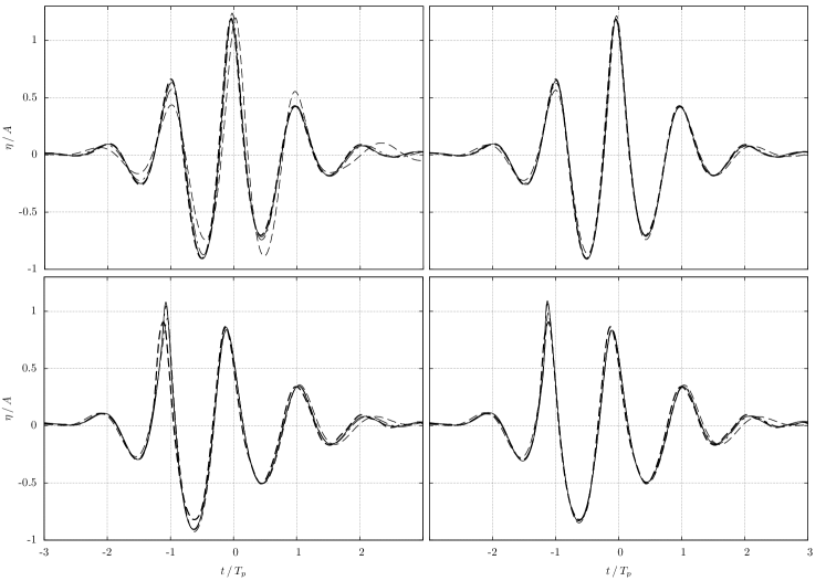
Figure 4: Convergence of time history of surface elevation for a wave group at $x=0$. Experiment (thick dashed) and Lagrangian solver: $N_{x}=101$ (dashed); $N_{x}=201$ (dash-dotted); $N_{x}=401$ (solid); $N_{z}=11$. Top – $A=5$ cm without (left) and with (right) dispersion correction. Bottom – $A=7.5$ cm, breaking control without (left) and with (right) crest correction.

We reconstruct the experimental setup using a numerical wave tank based on the previously described Lagrangian numerical model. The dimensions of the NWT are the same as the dimensions of the experimental tank. The wave is generated by implementing the boundary condition (6) on the right boundary of the computational domain with the paddle displacement recorded in the experiment. To account for gaps between the paddle and walls and bottom of the experimental flume we reduce the actual paddle displacement by $18.5\%$. The surface displacement damping term in (5) is activated near the tank wall opposite the wavemaker to absorb the reflections. Calculations are performed for all experimental cases, including three amplitudes and 4 phase shifts, and repeated with different time steps and horizontal and vertical numbers of mesh points. The time step has been reduced with an increasing number of horizontal mesh points to maintain the dispersion errors due to temporal and spatial discretisation given by (11) approximately equal to each other. This provides uniform convergence by both parameters. The summary of parameters for numerical cases is given in Table 1.

The convergence is tested using a $L_{2}$ norm of the difference between the experimental and calculated spectral components of the surface elevation at the linear focus point $x=0$. The norms for spectral amplitudes and phases are calculated as

$$||E(a)||=\sqrt{\sum_{n}(a_{n}-a_{n_{\mathrm{EXP}}})^{2}}\,;\quad||E(\phi)||=\sqrt{\sum_{n}(\phi_{n}-\phi_{n_{\mathrm{EXP}}})^{2}}\,,$$ (12)

where the sum is taken over discrete spectral components in the range $0.5\,\mathrm{Hz}<f<1.5\,\mathrm{Hz}$ from the set generated by the wavemaker ($n=32\dots 96$), where amplitude components are large enough not to be affected by experimental errors. It should be noted that full convergence of the calculated results to the experimental measurements can not be expected. The numerical model is based on a set of assumptions that are satisfied with limited precision. In addition, the measurements are also subject to accuracy limitations and experimental errors. Therefore, the difference between the experimental and numerical results converges to a certain small value and does not change with an additional increase in the resolution of the numerical model.

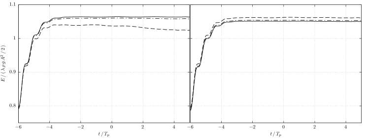
Figure 5: Convergence of the normalised total energy for the Lagrangian solver with dispersion correction. $A=5$ cm. Left – increasing horizontal mesh resolution: $N_{x}=101$ (dashed); $N_{x}=201$ (dash-dotted); $N_{x}=401$ (solid); $N_{z}=11$. Right – increasing vertical mesh resolution: $N_{z}=11$ (dashed); $N_{z}=16$ (dash-dotted); $N_{z}=21$ (solid); $N_{x}=251$.

Selected results for the convergence tests are presented in Figures 3-5. As can be seen in the top row of Figure 3, the results with and without dispersion correction converge to the same solution. However, the introduction of a dispersion correction considerably increases the speed of convergence for both amplitudes and phases. The experimental results can be reproduced with sufficient accuracy for a relatively small number of horizontal mesh points and a relatively large time step. For a breaking wave (Figure 3, bottom row), the shape correction of the crest introduces a new physical process. For this reason, the numerical results with and without crest correction converge to different solutions, and the numerical result with the correction shows a much better comparison with the experiment. A general impression of convergence and accuracy of the different versions of the numerical model can be obtained from the graphs of the time history of surface elevation presented in Figure 4.

Figure 5 shows the behaviour of the total wave energy in the wave tank calculated for different temporal and horizontal resolutions and different resolutions of the vertical mesh. Reflection absorption is disabled for the energy tests. The energy is normalised by the energy of one wave length $\lambda$ of a linear regular wave with a frequency and amplitude equal to the peak spectral frequency and the linear amplitude of the focussed wave. The kinetic energy is calculated by numerical integration over the entire Lagrangian fluid domain using a bi-linear interpolation of the velocities of the fluid particles inside mesh cells. This provides the second order approximation of the integral with respect to the mesh resolution. According to (8), the error of the velocity profiles within the fluid domain, and thus the kinetic energy, is determined by the horizontal and vertical resolution of the mesh. The potential energy is calculated as the integral of the potential energy density on a free surface and it is not directly affected by the discretisation of the vertical mesh. As can be seen in the figure, the total energy in the tank increases up to $t/T_{p}\approx-4$ due to the energy generated by the wave paddle. For low horizontal mesh resolution, the dissipative term in the numerical dispersion relation leads to the reduction of the energy of the propagating wave. For higher resolutions, energy conservation is satisfied with high accuracy. The right graph of Figure 5 shows the rapid convergence of energy with increased vertical resolution. This includes both the convergence of the numerical integral used to calculate kinetic energy and the convergence of the numerical solution for wave kinematics, as indicated by expansion (8). Overall, the convergence tests show that the numerical results converge towards a solution, which approximates the experiment with a good accuracy. The implementation of the dispersion correction term greatly increases the convergence rate and provides accurate results with a smaller number of mesh points and a larger time step.

4 VoF model

In this paper we also use olaFlow [35], an open source Navier–Stokes model developed as a continuation of the work in [36]. The model is based on OpenFOAM [37]. It includes enhancements to generate and absorb waves with moving boundaries [25], which allows to replicate piston and flap type wavemakers.

4.1 Mathematical formulation

This computational fluid dynamics (CFD) model solves the three-dimensional Reynolds-Averaged Navier-Stokes (RANS) equations, for two incompressible phases (water and air). Both fluids are considered a continuum mixture in which free surface is tracked with the Volume of Fluid (VoF) technique [38]. The model solves the conservation of mass and momentum equations:

$$\nabla\cdot(\rho\,\bf{U})=0$$ (13)

$$\frac{\partial\rho\bf{U}}{\partial t}+\nabla\cdot(\rho\bf{UU})=-\nabla\it{p}^{*}-\bf{g}\cdot\bf{X}\,\nabla\rho+\nabla\cdot(\mu\nabla\bf{U}-\rho\overline{\bf{U}^{\prime}\bf{U}^{\prime}})+\sigma\kappa\bf{\nabla\alpha}$$ (14)

in which $\rho$ is the density of the fluid, $t$ is time, $\nabla$ is the vector differential operator $(\partial/\partial x,\partial/\partial y,\partial/\partial z)$ and $\bf{U}$ is the Reynolds averaged velocity vector, $p^{*}=p-\rho\,\bf{g}\cdot\bf{X}$ is the dynamic pressure, $\bf{g}$ is the acceleration due to gravity and $\bf{X}$ is the position vector.

The molecular dynamic viscosity of the fluid ($\mu$) and the Reynolds stresses ($\rho\overline{\bf{U}^{\prime}\bf{U}^{\prime}}$) constitute the viscous term. In RANS, the Reynolds stresses can be modelled by different turbulence closure models, which introduce a dynamic turbulent viscosity ($\mu_{t}$). Generally, the viscous term is written in terms of the effective dynamic viscosity $\mu_{\mbox{\tiny eff}}=\mu+\mu_{t}$. The last term in equation (14) introduces the surface tension force [39]. In this term, $\sigma$ is the surface tension coefficient, $\kappa$ is the curvature of the free surface, calculated as $\nabla\cdot{\bf{\nabla\alpha}}\,/\,{|\bf{\nabla\alpha}|}$, and $\alpha$ is the Volume of Fluid (VoF) indicator function, introduced next.

In VoF, a continuous indicator function $\alpha$ represents the amount of water per unit volume in a cell. Thus, 1 is a pure water cell, 0 is a pure air cell, and $0<\alpha<1$ belongs to the interface. The movement of the fluids is tracked by a conservative advection equation, which needs to be bounded between 0 and 1, to be conservative and to maintain a sharp interface. The VoF equation in OpenFOAM is as follows:

$$\frac{\partial\alpha}{\partial t}+\nabla\cdot(\alpha\bf{U})+\nabla\cdot[\alpha(1-\alpha)\bf{U}_{c}]=0$$ (15)

The last term in (15) is an artificial compression (anti-diffusion) term to prevent the spread of the interface [40], which occurs because the numerical solutions of advection equations often suffer from diffusion. Within this term, $\bf{U}_{c}$ is a compression velocity in the normal direction to the free surface, acting only at the interface. The reader is referred to [36] for a complete description. Since the fluid mixture can be defined with $\alpha$, any fluid properties like density ($\rho$) or viscosity ($\nu$,$\mu$) are calculated as a weighted average, e.g.:

$$\rho=\alpha\,\rho_{w}+(1-\alpha)\,\rho_{a}$$ (16)

where subindices $w$ and $a$ denote water and air, respectively.

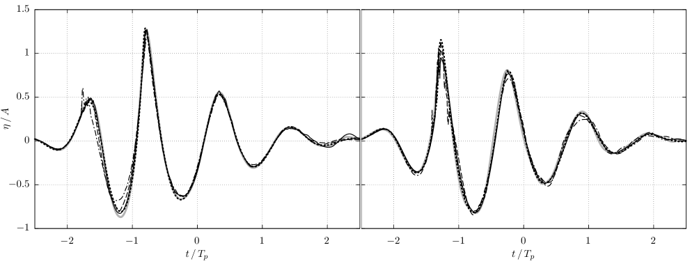
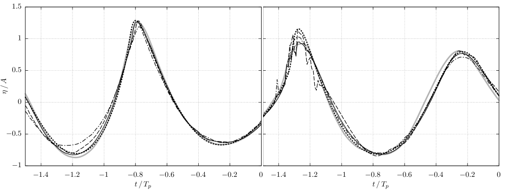
Figure 6: Surface elevation of a wave group at $x=0$. $A=7.5\,$cm. Left – pre-breaking ($\Delta\phi=\pi$). Right – post-breaking ($\Delta\phi=0$). Top – wave groups scale, Bottom – details around the main crest / trough. Experiment (solid grey), Lagrangian model (dotted), olaFlow with different mesh resolutions. Number of cells: $N=26832$ (dash-dotted); $N=105625$ (dashed); $N=413750$ (solid).

4.2 Model validation and convergence

The experiments are also reproduced in two dimensions using the VoF numerical wave tank olaFlow. The numerical setup is identical to that described in Section 3.4 for the Lagrangian model. The wave flume is $12.5$ m long and $0.56$ m high. Waves are generated on the right boundary with a piston-type wavemaker [25]. The wavemaker excursion has also been reduced by $18.5\%$ to account for losses occurring on the gaps between the paddle and the lateral and bottom walls of the experimental flume. The bottom wall of the flume carries a no-slip boundary condition (BC). Waves are absorbed actively at the boundary opposite to the wavemaker using boundary conditions described in [24]. Since CFD models excel in simulating nonlinear and wave breaking conditions, only the highest wave conditions ($A=7.5$ cm) were selected for two phase shifts $\Delta\phi=0$ and $\Delta\phi=\pi$.

Three meshes with different cell size have been tested in the convergence study. The most detailed mesh has a base cell size throughout the wave flume of $1\,$cm in the horizontal and vertical directions. A refinement region in which cells have high vertical resolution ($2.5$ mm) has been defined between $z=-0.08$ m and $z=0.10$ m (see Figure 1) to enhance the level of detail along the free surface. The resulting mesh is structured and non-conformal, and has a total of $N=413750$ square cells. The two other meshes have been built in a similar way, but with a maximum resolution half ($5$ mm) and one fourth ($1$ cm) of the cell size of the previous mesh. These configurations yield $N=105625$ and $N=26832$ cells, respectively. In the CFD simulations the time step is not fixed, but dynamically calculated to fulfil a maximum Courant number ($C_{o}$) of 0.15. All simulations have been run with the $k$-$\omega$ SST (shear stress transport) turbulence model defined in [41], which is especially suitable for wave simulations. The computational cost of each simulation varies due to the number of cells, which conditions the $C_{o}$, and physics involved (e.g. wave breaking). The simulations of 20 seconds in real time for the $N=26832$ mesh takes between 2.8 and 4.9 hours in a single core. The simulations for the $N=105625$ mesh take between 23.1 and 25.4 hours in two cores. The simulations for the $N=413750$ mesh take between 66.3 and 66.9 hours in four cores.

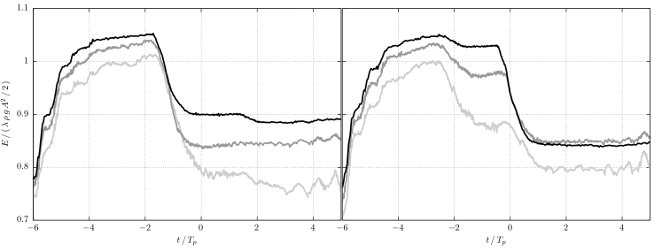
Figure 7: Normalised total energy of breaking waves calculated by olaFlow with different number of cells. $A=7.5$ cm. Left – phase shift $\Delta\phi=0$. Right – phase shift $\Delta\phi=\pi$. $N=26832$ (light grey); $N=105625$ (grey); $N=413750$ (black).

The convergence for olaFlow is evaluated in terms of the free surface elevation (Figure 6) and the normalised total energy of the wave flume (Figure 7). Figure 6 presents the free surface elevation at the centre of the tank $x=0$. Overall it can be seen that each refinement level in the CFD mesh yields a significant improvement in terms of agreement with the experimental results. The dash-dotted line corresponds to the lowest resolution ($N=26832$), and yields the maximum deviations with respect to the experiments. Furthermore, the coarsest mesh produces wave breaking artificially (top left panel, $t/T_{p}=-1.75$), as it is not present neither in the experiment nor in the refined cases. Additionally, wave breaking occurs significantly ahead of time for the $\Delta\phi=\pi$ case (bottom left panel, $t/T_{p}=-1.4$) for the lowest resolution. The mid and high resolution cases do not present such problems. In fact, the solid line solution captures remarkably well the complete profiles of the wave groups.

The total wave energy in Figure 7 has been obtained from a slightly different numerical setup than described above. Instead of absorbing the waves at the left end of the wave flume, the boundary has been replaced by a wall (no-slip BC) to prevent energy flowing out of the system, which would affect the energy calculations. Nevertheless, the reflected waves do not produce significant effects due to the length of the flume and short duration of the experiments. The total energy has been calculated as the sum of potential and kinetic energy, normalised by the energy of one wavelength of a linear regular wave, with the frequency and the amplitude equal to the peak spectral frequency and the linear focus amplitude of the wave group. Both potential and kinetic energy have been calculated as a cell-wise numerical integration over those cells within the domain that contain water ($\alpha>0.05$).

All the simulations in Figure 7 show oscillations on the initial ramp. These are created by the moving wavemaker, which is introducing energy to the system. Another common feature is that the cells resolution plays a significant role in reaching higher levels of energy before wave breaking. In the left panel ($\Delta\phi=0$), the three meshes predict wave breaking consistently after reaching the maximum value in total energy. In view of the maximum energy level and the energy level of the plateau after wave breaking, it can be observed that the higher the resolution, the lower the energy dissipation due to breaking. In the cases shown in the right panel ($\Delta\phi=\pi$), this last conclusion only holds initially, for the wave breaking event at $t/T_{p}=-2$. However, the main breaking event at $t/T_{p}=0$ shows the opposite behaviour, with increasing dissipation with increasing resolution. Generally, the dissipation in the leading breaking event decreases with higher resolutions, but it can increase in the following event because the wave loses less energy in the first event and remains more energetic when the second event takes place.

Overall, the results from the convergence tests presented in this section show a significant improvement for smaller cell sizes when compared against the experimental results. Also, the observations made are aligned with those in [42]. In their work they demonstrated that insufficient resolution and large $C_{o}$ lead to over-predictions of wave amplitude, leading to premature and more pronounced wave breaking [42].

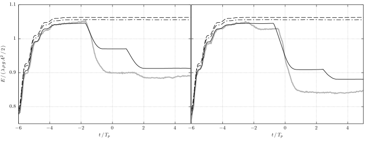
Figure 8: Normalised total wave energy for Lagrangian (black) and VoF (grey) solvers. Left – phase shift $\Delta\phi=0$. Right – phase shift $\Delta\phi=\pi$. $A=2.5$ cm (dashed); $A=5$ cm (dash-dotted) and $A=7.5$ cm (solid).

5 Results

The olaFlow model and the Lagrangian model are applied in this section to simulate the evolution of a steep wave group with a focus on modelling the wave breaking process. The calculations by the Lagrangian model are performed using a $401\times 16$ mesh and the time step $\delta t=0.0025$ sec. The mesh with 413750 cells and $C_{o}=0.15$ is used for the OpenFOAM computations. Figure 8 shows the evolution of the total wave energy for amplitude $A=7.5$ cm and phase shifts $\Delta\phi=0$ and $\Delta\phi=\pi$, which correspond to inverse wavemaker input signals. Plots for amplitudes of $A=2.5$ cm and $A=5$ cm calculated with the Lagrangian model are presented as a reference. The energy is normalised as described in Section 3.4. The wave energy increases from the initial zero level after the wavemaker starts operating. After the wavemaker stops at $t/T_{p}\approx-3$, the total energy remains constant until wave breaking occurs. As expected, the energy of non-breaking waves is the same for both phase shifts.

For $\Delta\phi=0$ the Lagrangian model predicts two breaking events of similar intensity, which are symmetrical with respect to $t=0$ and, therefore, with respect to the centre of the tank. This qualitative behaviour is confirmed by experimental observations. In contrast, olaFlow predicts a strong initial breaking event and a small secondary breaking event. For $\Delta\phi=\pi$, the Lagrangian results demonstrate an intensive breaking event near the centre of the tank close to $t=0$ and a smaller breaking event near $t/T_{p}=2.5$. The olaFlow model presents a small breaking event at $t/T_{p}\approx-2.5$ prior to the main one. Only one major breaking event in the centre of the reservoir was observed in the experiment in this case. For both cases the VoF model predicts higher overall energy dissipation. The convergence results of the VoF model for $\Delta\phi=0$ presented in Figure 7 show that the increase in mesh resolution results in decreasing intensity of the main breaking event and the development of a smaller second breaking event. For $\Delta\phi=\pi$, the higher resolution results in the decreasing intensity of the first breaking event and the development of a strong breaking event at $t=0$. It should be noted, that VoF breaking results are not fully converged. It is reasonable to assume that a further increase in mesh resolution will lead to the observed qualitative breaking behaviour with two symmetric breaking events for $\Delta\phi=0$ and a single strong break event at $t=0$ for $\Delta\phi=\pi$. Given the computational time required to obtain these results, it was found impractical pursuing an additional level of resolution. For the Lagrangian solver, the difference with the observed breaking behaviour is due to the application of the nonphysical heuristic breaking model, which requires an adjustment of the parameters to obtain the best performance for each individual case. Detailed calibration of the Lagrangian model for different breaking conditions is outside the scope of the present paper.

In the reminder of this section we perform a detailed comparison of the behaviour of the two models around the breaking crest. We focus our attention to the large breaking event at the centre of the tank and consider the wave with $A=7.5\,$cm and $\Delta\phi=\pi$. Figure 9 shows the time history of wave crest elevation at three locations along the tank. The corresponding wave profiles can be seen in Figure 10. The difference between measured and calculated wave crests can be observed in Figure 9 near the top of the crest. It should be noted that for very steep wave peaks the experimental measurements by wave probes are unreliable. This is due to the high-speed flow at the crest, which creates a cavity around the wires of the wave probe, resulting in a reduction in the recorded crest elevation. However, for the main part of the crest, the calculated and experimental results are compared with good accuracy. The rounded end of the overturning wave observed in Figure 10 is explained by surface tension, which produces a considerable effect given the relatively small experimental scale. For the initial phase of wave breaking, there is a very good agreement between the Lagrangian model without the breaking model and olaFlow. However, olaFlow predicts a slightly faster development of the breaker. These differences can be caused by many reasons such as insufficient mesh resolution at the crest for the VoF model or the exclusion of air effects by the Lagrangian model. Since the breaking process is extremely sensitive to small disturbances, the achieved level of comparison can be considered satisfactory.

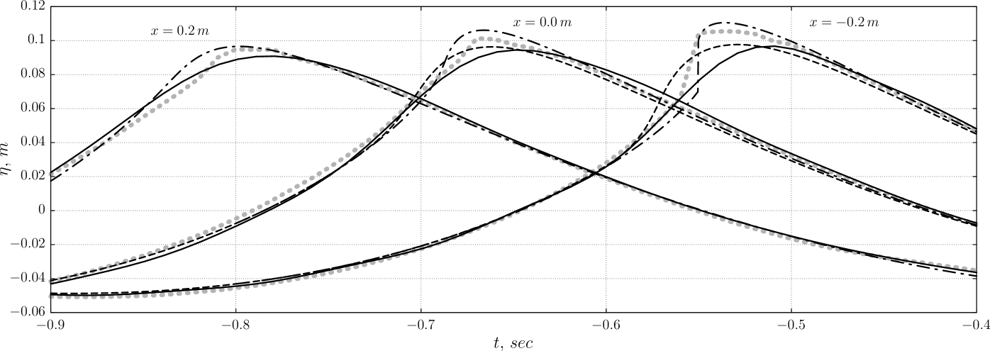
Figure 9: Time histories of wave crest evolution at different positions along the flume, $A=7.5$ cm, $\Delta\phi=\pi$. Experiment (solid); VoF model (grey points); Lagrangian model (dash-dotted); Lagrangian model with breaking model (dashed).

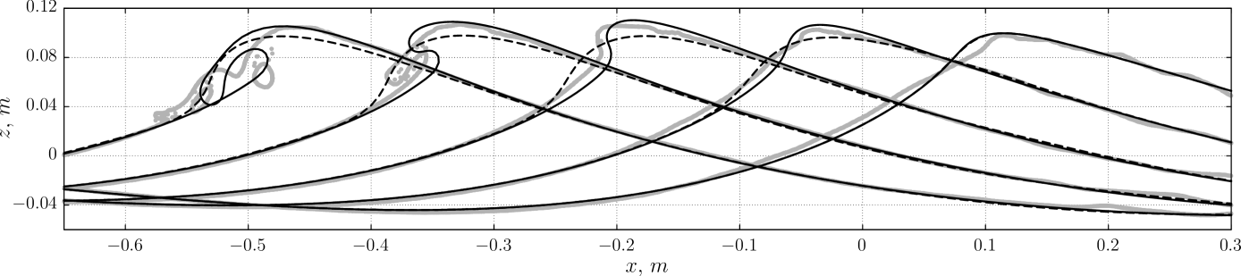
Figure 10: Breaking crest evolution between $t=-0.76$ sec and $t=-0.36$ sec. VoF model (thick grey); Lagrangian model (solid); Lagrangian model with breaking model (dashed).

For the wave peak at $x=0.2\,$m, the Lagrangian breaking model is not yet activated and thus the Lagrangian solutions with and without the breaking model are identical. At $x=0$, the top of the wave crest begins to deform. It moves faster than the main body of the crest and eventually overturns. At this stage, the damping term of the breaking model is activated, as illustrated by the differences in the crest shape with and without the breaking model. Further in the tank, at $x=-0.2\,$m, the top of the crest begins to overturn and a vertical front develops. The shape of the crest computed with the active breaking model is seen to differ considerably from the shape of the freely-evolving crest. However, the main differences are located near the top of the crest, while other parts of the wave are unaffected by the breaking model. Calculations without the breaking model are continued until the self contact of the overturning wave at $t=-0.36\,$sec (Figure 10). After that, the results produced by the Lagrangian model without the breaking model are not physically meaningful. The breaking model, on the other hand, does not show overturning, but allows further calculations beyond this point.

In the last two profiles ($t=-0.46\,$sec and $t=-0.36\,$sec), olaFlow shows forming of a large air pocket and smaller bubbles. The model also predicts the wave crest bouncing from the free surface of the main water body, creating a second plunger. However, it must be noted that the olaFlow simulation is 2D, whereas wave breaking is typically a highly 3D process. This means that, for example, trapped air will only be able to escape upward, whereas in 3D it might also escape sideways. In addition, the mesh resolution achieved in olaFlow calculations does not provide full convergence of breaking results. Therefore, the present solution must be regarded with the limitations inherent to 2D modelling and insufficient mesh resolution. Unlike the VoF model, the Lagrangian model is not able to simulate the air entrapment. However, as can be seen in Figure 10, the solution with the breaking model reproduces the shape of the breaking wave crest relatively well, and provides a good starting point for subsequent simulations of the post-breaking wave.

Examples of horizontal and vertical velocity profiles at the wave crest and on the front and rear slopes are given in Figure 11. The profiles are presented at the moment when surface elevation reaches its maximum at $x=0$ and the crest starts overturning. There is a good general agreement between the profiles calculated by olaFlow and the Lagrangian model without the breaking model. The higher peak velocity for the VoF model is consistent with the previous observation of faster crest deformation. The difference between the velocities calculated by the Lagrangian model with and without the breaking model can be observed near the top of the wave crest but disappears rapidly everywhere else. It is important to note the good degree of agreement between velocity profiles and surface elevation calculated by the Lagrangian model with the breaking model and olaFlow for the region outside the immediate vicinity of the breaking crest.

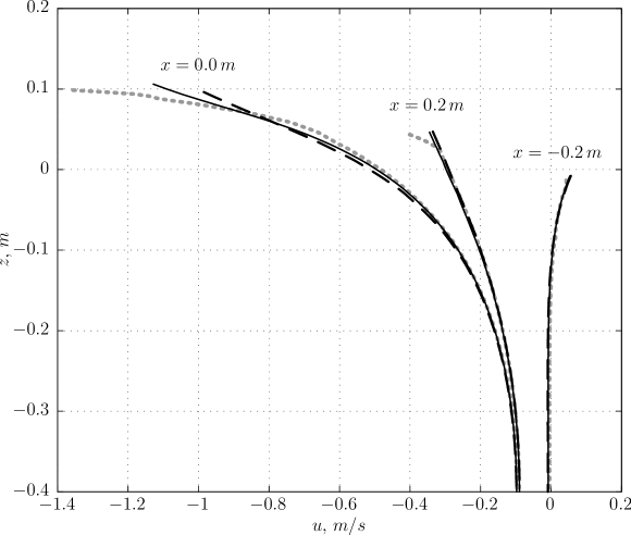
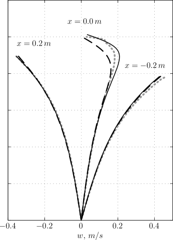
Figure 11: Horizontal (left) and vertical (right) velocity component profiles at $t=-0.665$ and different positions along the flume. VoF model (dotted grey); Lagrangian model (solid); Lagrangian model with breaking model (dashed). The time corresponds to the maximal surface elevation at $x=0$.

6 Discussion and conclusions

The main result of the paper is the development of a fully Lagrangian numerical model and its application to the evolution of steep wave groups with breaking. The model is able to simulate the long-term evolution of highly nonlinear waves and to calculate wave profiles and kinematics close to spilling breaking. A 4-parametric dissipative breaking model is introduced to prevent the breakdown of computations, which usually follows the breaking onset. To improve the accuracy of modelling of the long-term evolution of travelling waves, a dispersion correction term is introduced to the free surface boundary condition, which increases the order of approximation of the dispersion relation.

The results of Lagrangian calculations for surface elevation are validated against wave flume experiments and for surface elevation and kinematics against numerical results obtained by a VoF model. OlaFlow OpenFOAM realisation of VoF with a recent addition of a realistic method of wave generation with a piston type wavemaker [24, 25] is used in this paper. Although this may seem trivial, before introducing this addition, comparing OpenFOAM computations for water waves with experiments and results of other numerical models was not an obvious task, mainly because of the different methods of wave generation. After introducing a realistic wavemaker, it became possible to create an OpenFOAM wave tank replicating the actual experimental wave flume. Since the same experimental flume is simulated by the OpenFOAM model and the Lagrangian solver, the direct comparison of the experimental and numerical results becomes straightforward.

For a steep non-breaking wave group, both the OpenFOAM results and the results of the Lagrangian model with dispersion correction demonstrate a perfect match with experimental surface elevation measurements. An equally good comparison up to breaking onset is also reported for the steepest wave group tested. Post breaking behaviour of the wave group is not simulated that well by either model (Figure 6). For the Lagrangian solver this is caused by the application of the nonphysical heuristic breaking model, which requires selection of model parameters. For the VoF solver, this is mainly due to an insufficient mesh resolution in the vicinity of the breaking crest. Another reason is the application of a two-dimensional mesh, which does not allow to resolve the three-dimensional details of the formation and the evolution of the turbulent breaking roller. It should be noted that for both models, the difference is mainly concentrated around the breaking crest and that the overall evolution after the breaking is simulated relatively well.

Further comparison between the numerical results is performed for parameters not measured in the experiment. Simulations of an overturning crest with olaFlow and the Lagrangian model without the breaking model demonstrate a good agreement (Figures 9, 10). For the Lagrangian model with the breaking model the difference of the profiles is localised in a small area around the crest and disappears for the rest of the wave profile. The same can be said about velocity profiles under the crest just before the breaking (Figure 11). There is a good agreement between velocity profiles for the VoF model and for the Lagrangian model without the breaking model. For the Lagrangian model with suppressed breaking, the difference between the calculated velocities can only be observed in the vicinity of the crest. Overall, when compared with olaFlow computations of wave breaking, the results of Lagrangian calculations with the breaking model demonstrate plausible behaviour with intensive energy dissipation (Figure 8).

Figure 12: Computation time for modelling of 20 sec of wave propagation by the Lagrangian solver on a single 2.4 GHz CPU for different mesh size: $N_{z}=11$ (solid); $N_{z}=16$ (dashed); $N_{z}=21$ (dash-dotted).

Computational efficiency of the Lagrangian solver is important for its applicability to large-scale problems, especially in 3D. In the implicit time marching scheme implemented in the Lagrangian solver, the most time consuming element is the inversion of a Jacobi matrix used by the Newton iterations for solving nonlinear grid equations. The required calculation time grows fast with increasing matrix dimension, which is proportional to the square of the product of dimensions of a numerical mesh. For a matrix inversion algorithm used in this work, the inversion time is approximately proportional to the square of the dimension of the matrix. For a 2D problem with a constant value of $N_{z}$ much smaller than $N_{x}$, the matrix dimension is proportional to $N_{x}$. To provide a uniform discretisation error in space and time, the value of time step should be proportional to $\delta x$, which implies that the number of steps is proportional to $N_{x}$. Thus, the overall calculation time grows with a rate proportional to $N_{x}^{3}$, as illustrated by Figure 12. For an explicit method, like the one used in olaFlow, the computational time estimated in the same way is proportional to $N_{x}^{2}$. Due to better numerical stability, the Lagrangian model uses considerably larger time step. Moreover, it requires less horizontal points to resolve the free surface since the latter is well defined by the upper boundary of the Lagrangian computational domain. As a result, the Lagrangian model requires much less spatial points and less time steps to obtain a stable solution of the same accuracy as the OpenFOAM model.

If the number of mesh points increases due to a larger computational domain or high mesh resolution, the computational time for the Lagrangian model grows much faster than that for the OpenFOAM model. For a sufficiently large number of points, the Lagrangian model loses its advantage in computational efficiency. This disadvantage of the Lagrangian model becomes crucial for 3D problems, which restricts the applicability of the current version of the Lagrangian solver. High demand for computational resources for large scale problems is a well recognised disadvantage of implicit schemes, which often outweighs their advantages in numerical stability. The radical method of increasing computational efficiency is using parallel computing. Implicit solvers, like the one used in the Lagrangian model, have a single standard time-consuming operation and are therefore suitable for efficient parallelisation. A parallel version of an implicit solver can be created with minimal changes to the original code by replacing a matrix inversion subroutine with a parallel analogue. This feature is particularly useful in light of recent advances in GPU-based matrix inversion algorithms, which are much faster than conventional parallelisation using multiple CPUs [43].

The good agreement between the velocity profiles and the surface elevation calculated by the Lagrangian model and the olaFlow model makes it possible to use them to create a hybrid model in order to reach a new qualitative level of efficiency and accuracy of modelling. The elements of a hybrid model are used to simulate different parts of the overall process. The Lagrangian model more efficiently simulates long-term wave evolution than the VoF model. However, a non-physical breaking model is needed to continue the calculations after wave breaking. On the other hand, the VoF model is able to directly simulate the breaking process, but a high mesh resolution is required. It is therefore advantageous to create a hybrid model combining the Lagrangian model to simulate the wave group evolution and the VoF model to simulate the details of the breaking process. More specifically, the VoF model to be used to model the small region around the breaking crest, which allows to obtain a high mesh resolution with a relatively small number of mesh points and therefore with a low computational cost. As a first step, the Lagrangian and VoF coupled models were recently applied to fluid-structure interaction problems, which requires simpler coupling techniques, compared to a hybrid breaking model [44, 23].

In summary, the results presented in the paper demonstrate high quality validation for both numerical models. The Lagrangian is able to simulate the evolution of steep wave groups before and after breaking. The accuracy achieved by the Lagrangian model is comparable to that achieved by a VoF model but the required computational resources are considerably smaller. The level of agreement between the surface elevation and the velocities around a breaking crest, calculated by both models, makes them promising elements of a more efficient hybrid model.

References

- [1] Lindgren G. 1970 Some properties of a normal process near a local maximum. Ann. Math. Stat. 41, 1870–1883.
- [2] Phillips O, Gu D, Donelan M. 1993 Expected structure of extreme waves in a Gaussian sea. Part I: Theory and SWADE buoy measurements. Journal of Physical Oceanography 23, 992–1000.
- [3] Christou M, Ewans K. 2014 Field measurements of rogue water waves. Journal of Physical Oceanography 44, 2317–2335.
- [4] Tromans PS, Anatruk A, Hagemeijer P. 1991 New model for the kinematics of large ocean waves application as a design wave. Proceedings of the First International Offshore and Polar Engineering Conference pp. 64–71.
- [5] Chen L, Zang J, Hillis A, Morgan G, Plummer A. 2014 Numerical investigation of wave–structure interaction using OpenFOAM. Ocean Engineering 88, 91–109.
- [6] Hu ZZ, Greaves D, Raby A. 2016 Numerical wave tank study of extreme waves and wave-structure interaction using OpenFoam. Ocean Engineering 126, 329–342.
- [7] Kim SH, Yamashiro M, Yoshida A. 2010 A simple two-way coupling method of BEM and VOF model for random wave calculations. Coastal Engineering 57, 1018–1028.
- [8] Sriram V, Ma Q, Schlurmann T. 2014 A hybrid method for modelling two dimensional non-breaking and breaking waves. Journal of Computational Physics 272, 429–454.
- [9] Narayanaswamy M, Crespo AJC, Gómez-Gesteira M, Dalrymple RA. 2010 SPHysics-FUNWAVE hybrid model for coastal wave propagation. Journal of Hydraulic Research 48, 85–93.
- [10] Landrini M, Colagrossi A, Greco M, Tulin M. 2012 The fluid mechanics of splashing bow waves on ships: A hybrid BEM–SPH analysis. Ocean Engineering 53, 111–127.
- [11] Tsai W, Yue DKP. 1996 Computation of Nonlinear Free-Surface Flows. Ann. Rev. Fluid Mech. 28, 249–278.
- [12] Grilli S, Guyenne P, Dias F. 2001 A fully non-linear model for three-dimensional overturning waves over an arbitrary bottom. International Journal for Numerical Methods in Fluids 35, 829–867.
- [13] Gomez-Gesteira M, Rogers BD, Dalrymple RA, Crespo AJ. 2010 State-of-the-art of classical SPH for free-surface flows. Journal of Hydraulic Research 48, 6–27.
- [14] Violeau D, Rogers BD. 2016 Smoothed particle hydrodynamics (SPH) for free-surface flows: past, present and future. Journal of Hydraulic Research 54, 1–26.
- [15] Brennen C, Whitney AK. 1970 Unsteady, free surface flows; solutions employing the Lagrangian description of the motion. In 8th Symposium on Naval Hydrodynamics pp. 117–145. Office of Naval Research.
- [16] Hirt C, Cook J, Butler T. 1970 A Lagrangian method for calculating the dynamics of an incompressible fluid with free surface. Journal of Computational Physics 5, 103–124.
- [17] Chan RKC. 1975 A Generalized Arbitrary Lagrangian-Eulerian Method for Incompressible Flows with Sharp Interfaces. Journal of Computational Physics 17, 311–331.
- [18] Braess H, Wriggers P. 2000 Arbitrary Lagrangian Eulerian finite element analysis of free surface flow. Computational Methods in Applied Mechhanics and Engineering 190, 95–109.
- [19] Souli M, Benson DJ. 2013 Arbitrary Lagrangian Eulerian and Fluid-Structure Interaction: Numerical Simulation. Wiley-ISTE.
- [20] Buldakov E. 2013 Tsunami generation by paddle motion and its interaction with a beach: Lagrangian modelling and experiment. Coastal Engineering 80, 83–94.
- [21] Buldakov E. 2014 Lagrangian modelling of fluid sloshing in moving tanks. Journal of Fluids and Structures 45, 1–14.
- [22] Buldakov E, Stagonas D, Simons R. 2015 Langrangian numerical wave-current flume. In Proceedings of 30th International Workshop on Water Waves and Floating Bodies pp. 25–28 Bristol, UK.
- [23] Chen L, Stagonas D, Santo H, Buldakov E, Taylor P, Zang J. Submitted. Numerical modelling of interactions of waves and sheared currents with a surface piercing vertical cylinder. Coastal Engineering.
- [24] Higuera P, Lara JL, Losada IJ. 2013 Realistic wave generation and active wave absorption for Navier–Stokes models. Coastal Engineering 71, 102–118.
- [25] Higuera P, Losada IJ, Lara JL. 2015 Three-dimensional numerical wave generation with moving boundaries. Coastal Engineering 101, 35–47.
- [26] Buldakov E, Stagonas D, Simons R. 2017 Extreme wave groups in a wave flume: Controlled generation and breaking onset. Coastal Engineering 128, 75–83.
- [27] Buldakov E, Taylor P, Eatock Taylor R. 2006 New asymptotic description of nonlinear water waves in Lagrangian coordinates. Journal of Fluid Mechanics 562, 431–444.
- [28] Keller HB. 1971 A new difference scheme for parabolic problems. In Numerical Solution of Partial Differential Equations, II (SYNSPADE 1970) (Proc. Sympos., Univ. of Maryland, College Park, Md., 1970) pp. 327–350. New York: Academic Press.
- [29] NAG. 2016 NAG Library Manual, Mark 26. The Numerical Algorithms Group Ltd Oxford, UK.
- [30] Dommermuth D, Yue D. 1987 Numerical simulations of nonlinear axisymmetric flows with a free surface. Journal of Fluid Mechanics 178, 195–219.
- [31] Subramani A, Beck R, Schultz W. 1998 Suppression of wave breaking in nonlinear water wave computations. In Proceedings of 13th International Workshop on Water Waves and Floating Bodies pp. 139–142 Alphen aan den Rijn, The Netherlands.
- [32] Guignard S, Grilli S. 2001 Modeling of wave shoaling in a 2D-NWT using a spilling breaker model. In Proceedings of the International Offshore and Polar Engineering Conference vol. 3 pp. 116–123.
- [33] Tian Z, Perlin M, Choi W. 2012 An eddy viscosity model for two-dimensional breaking waves and its validation with laboratory experiments. Physics of Fluids 24, 036601–1 – 036601–23.
- [34] Seiffert BR, Ducrozet G. 2018 Simulation of breaking waves using the high-order spectral method with laboratory experiments: wave-breaking energy dissipation. Ocean Dynamics 68, 65–89.
- [35] Higuera P. 2017 olaFlow: CFD for waves. https://doi.org/10.5281/zenodo.1297013 .
- [36] Higuera P. 2015 Application of computational fluid dynamics to wave action on structures. PhD thesis University of Cantabria.
- [37] Weller H, Tabor G, Jasak H, Fureby C. 1998 A tensorial approach to computational continuum mechanics using object-oriented techniques.. Computers in Physics 12, 620–631.
- [38] Hirt CW, Nichols BD. 1981 Volume of fluif (VOF) method for the dynamics of free boundaries.. Journal of Computational Physics 39, 201–225.
- [39] Brackbill JU, Kothe DB, Zemach C. 1992 A continuum method for modeling surface tension.. Journal of Computational Physics 100, 335–354.
- [40] Berberovic E, van Hinsberg NP, Jakirlic S, Roisman IV, Tropea C. 2009 Drop impact onto a liquid layer of finite thickness: Dynamics of the cavity evolution.. Physical Review E 79, 036306.
- [41] Devolder B, Troch P, Rauwoens P. 2018 Performance of a buoyancy-modified k-omega and k-omega SST turbulence model for simulating wave breaking under regular waves using OpenFOAM.. Coastal Engineering 138, 49–65.
- [42] Vyzikas T, Stagonas D, Buldakov E, Greaves D. 2018 The evolution of free and bound waves during dispersive focusing in a numerical and physical flume. Coastal Engineering 132, 95–109.
- [43] Sharma G, Agarwala A, Bhattacharya B. 2013 A fast parallel Gauss Jordan algorithm for matrix inversion using CUDA. Computers & Structures 128, 31–37.
- [44] Higuera P, Buldakov E, Stagonas D. 2018 Numerical modelling of wave interaction with an FPSO using a combination of OpenFOAM and Lagrangian models. In Proceedings of the 28th International Ocean and Polar Engineering Conference pp. 1486–1491 Sapporo, Japan.