2018 Update on $\varepsilon_{K}$ with lattice QCD inputs

Abstract:

We present updated results for $\varepsilon_{K}$ determined directly from the standard model (SM) with lattice QCD inputs such as $\hat{B}_{K}$, $|V_{cb}|$, $|V_{us}|$, $\xi_{0}$, $\xi_{2}$, $\xi_{\text{LD}}$, $F_{K}$, and $m_{c}$. We find that the standard model with exclusive $|V_{cb}|$ and other lattice QCD inputs describes only 70% of the experimental value of $|\varepsilon_{K}|$ and does not explain its remaining 30%, which leads to a strong tension in $|\varepsilon_{K}|$ at the $4\sigma$ level between the SM theory and experiment. We also find that this tension disappears when we use the inclusive value of $|V_{cb}|$ obtained using the heavy quark expansion based on QCD sum rules.

1 Introduction

This paper is a brief summary of our previous paper [1]. This paper is also an update of our previous papers [2, 3, 4].

2 Input parameters: $|V_{cb}|$ and $\xi_{0}$

In Table 1, we present updated results for both exclusive $|V_{cb}|$ and inclusive $|V_{cb}|$. Recently, HFLAV reported them in Ref. [5]. The results for exclusive $|V_{cb}|$ are obtained using lattice QCD results for the semileptonic form factors of Refs. [6, 7, 8]. Here, we use the combined results (ex-combined) for exclusive $|V_{cb}|$ and the results of the $1S$ scheme for inclusive $|V_{cb}|$ to evaluate $\varepsilon_{K}$. For more details on $|V_{cb}|$ and the related caveats, refer to Ref. [1].

channel	value	Ref.
$B\to D^{*}\ell\bar{\nu}$	$39.05(47)(58)$	[5, 6]
$B\to D\ell\bar{\nu}$	$39.18(94)(36)$	[5, 7]
$|V_{ub}|/|V_{cb}|$	$0.080(4)(4)$	[5, 8]
ex-combined	$39.13(59)$	[5]

(a) Results for exclusive $|V_{cb}|$.

channel	value	Ref.
kinetic scheme	$42.19(78)$	[5]
1S scheme	$41.98(45)$	[5]
in-combined	$42.03(39)$	[1]

(b) Results for inclusive $|V_{cb}|$.

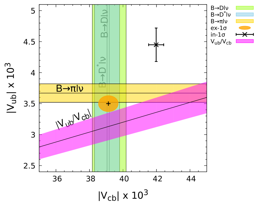
(a) $|V_{cb}|$ versus $|V_{ub}|$.

Table 1: $|V_{cb}|$: (1(b)) exclusive $|V_{cb}|$, (1(b)) inclusive $|V_{cb}|$, and (1(a)) $|V_{cb}|$ versus $|V_{ub}|$.

The absorptive part of long distance effects on $\varepsilon_{K}$ is parametrized into $\xi_{0}$.

$$\xi_{0} =\frac{\mathrm{Im}\,A_{0}}{\mathrm{Re}\,A_{0}},\qquad\xi_{2}=\frac{\mathrm{Im}\,A_{2}}{\mathrm{Re}\,A_{2}},\qquad\mathrm{Re}\,\left(\frac{\varepsilon^{\prime}}{\varepsilon}\right)=\frac{\omega}{\sqrt{2}|\varepsilon_{K}|}(\xi_{2}-\xi_{0})\,.$$ (1)

There are two independent methods to determine $\xi_{0}$ in lattice QCD: one is the indirect method and the other is the direct method. In the indirect method, one can determine $\xi_{0}$ using Eq. (1) with lattice QCD input $\xi_{2}$ and with experimental results for $\varepsilon^{\prime}/\varepsilon$, $\varepsilon_{K}$, and $\omega$. In the direct method, one can determine $\xi_{0}$ directly using lattice QCD results for $\mathrm{Im}\,A_{0}$ combined with experimental results for $\mathrm{Re}\,A_{0}$. In Table 2 (2(b)), we summarize results for $\xi_{0}$ calculated by RBC-UKQCD using the indirect and direct methods. Here, we use the results of the indirect method for $\xi_{0}$ to evaluate $\varepsilon_{K}$.

In Ref. [9], RBC-UKQCD also reported the S-wave scattering phase shift for the $I=0$ channel: $\delta_{0}=23.8(49)(12)$, which is different from those of the dispersion relations [10, 11] by $\approx 3\sigma$. In Ref. [12], they have accumulated higher statistics to obtain $\delta_{0}=19.1(25)(12)$, which is about $5\sigma$ different from those of the dispersion analyses. They introduce a $\sigma$ operator and make all possible combinations with the $\sigma$ and $\pi-\pi$ operators. Then, RBC-UKQCD has obtained $\delta_{0}=32.8(12)(30)$ which is consistent with those of the dispersion relations. These results are presented in Table 2 (2(b)) and Figure 2 (2(a)).

method	$\xi_{0}$	Ref.
indirect	$-1.63(19)\times 10^{-4}$	[13]
direct	$-0.57(49)\times 10^{-4}$	[9]

(a) $\xi_{0}$

Collaboration	$\delta_{0}$	Ref.
RBC-UKQCD-15	$23.8(49)(12){}^{\circ}$	[9]
RBC-UKQCD-18	$32.8(12)(30){}^{\circ}$	[12]
KPY-2011	39.1(6)∘	[11]
CGL-2001	39.2(15)∘	[10, 14]

(b) Results for $\delta_{0}$

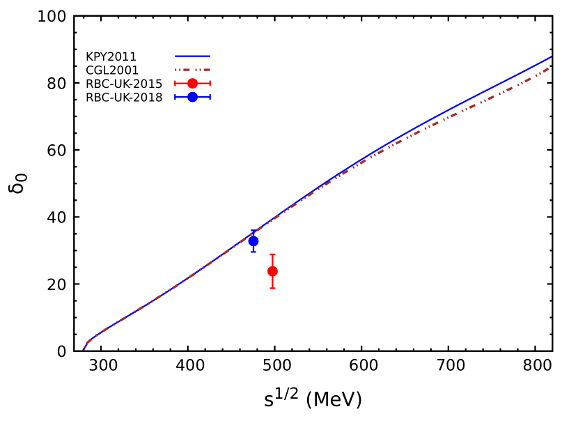
(a) $\delta_{0}$

Table 2: The absorptive long distance effect $\xi_{0}$ and S-wave $I=0$ scattering phase shift $\delta_{0}$.

3 Input parameters: Wolfenstein parameters, $\hat{B}_{K}$, $\xi_{\text{LD}}$, and others

In Table 3 (3(a)), we summarize the Wolfenstein parameters on the market. The CKMfitter and UTfit collaboration provide the Wolfenstein parameters determined by the global unitarity triangle (UT) fit. Unfortunately, $\varepsilon_{K}$, $\hat{B}_{K}$, and $|V_{cb}|$ are used as inputs to the global UT fit, which leads to unwanted correlation with $\varepsilon_{K}$. We want to avoid this correlation, and so take another input set from the angle-only fit (AOF) suggested in Ref. [15]. The AOF does not use $\varepsilon_{K}$, $\hat{B}_{K}$, and $|V_{cb}|$ as input to determine the UT apex $(\bar{\rho},\bar{\eta})$. Here the $\lambda$ parameter is determined from $|V_{us}|$ which is obtained from the $K_{\ell 2}$ and $K_{\ell 3}$ decays using lattice QCD results for the form factors and decay constants. The $A$ parameter is determined from $|V_{cb}|$.

WP	CKMfitter		UTfit		AOF
$\lambda$	$0.22509(29)$	[16]	$0.22497(69)$	[17]	$0.2248(6)$	[18]
$\bar{\rho}$	$0.1598(76)$	[16]	$0.153(13)$	[17]	$0.146(22)$	[19]
$\bar{\eta}$	$0.3499(63)$	[16]	$0.343(11)$	[17]	$0.333(16)$	[19]

(a) Wolfenstein parameters

Input	Value	Ref.
$\eta_{cc}$	$1.72(27)$	[3]
$\eta_{tt}$	$0.5765(65)$	[20]
$\eta_{ct}$	$0.496(47)$	[21]

(b) $\eta_{ij}$

Table 3: (3(a)) Wolfenstein parameters and (3(b)) QCD corrections: $\eta_{ij}$ with $i,j=c,t$.

In the FLAG review [22], they present lattice QCD results for $\hat{B}_{K}$ with $N_{f}=2$, $N_{f}=2+1$, and $N_{f}=2+1+1$. Here, we use the results for $\hat{B}_{K}$ with $N_{f}=2+1$, which is obtained by taking a global average over the four data points from BMW 11 [23], Laiho 11 [24], RBC-UKQCD 14 [25], and SWME 15 [26]. In Table 4 (4(a)), we present the FLAG 17 result for $\hat{B}_{K}$ with $N_{f}=2+1$, which is used to evaluate $\varepsilon_{K}$.

Collaboration	Ref.	$\hat{B}_{K}$
SWME 15	[26]	$0.735(5)(36)$
RBC/UKQCD 14	[25]	$0.7499(24)(150)$
Laiho 11	[24]	$0.7628(38)(205)$
BMW 11	[23]	$0.7727(81)(84)$
FLAG 17	[22]	$0.7625(97)$

(a) $\hat{B}_{K}$

Input	Value	Ref.
$G_{F}$	$1.1663787(6)\times 10^{-5}$ GeV-2	[18]
$M_{W}$	$80.385(15)$ GeV	[18]
$m_{c}(m_{c})$	$1.2733(76)$ GeV	[27]
$m_{t}(m_{t})$	$163.65(105)(17)$ GeV	[1]
$\theta$	$43.52(5)^{\circ}$	[18]
$m_{K^{0}}$	$497.611(13)$ MeV	[18]
$\Delta M_{K}$	$3.484(6)\times 10^{-12}$ MeV	[18]
$F_{K}$	$155.6(4)$ MeV	[18]

(b) Other parameters

Table 4: (4(a)) Results for $\hat{B}_{K}$ and (4(b)) other input parameters.

The dispersive long distance (LD) effect is defined as

$$\xi_{\text{LD}} =\frac{m^{\prime}_{\text{LD}}}{\sqrt{2}\Delta M_{K}}\,,\qquad m^{\prime}_{\text{LD}}=-\mathrm{Im}\,\left[\mathcal{P}\sum_{C}\frac{\langle\overline{K}^{0}\lvert H_{\text{w}}\rvert C\rangle\langle C\lvert H_{\text{w}}\rvert K^{0}\rangle}{m_{K^{0}}-E_{C}}\right]$$ (2)

If the CPT invariance is well respected, the overall contribution of the $\xi_{\text{LD}}$ to $\varepsilon_{K}$ is about $\pm 2\%$.

Lattice QCD tools to calculate $\xi_{\text{LD}}$ are well established in Refs. [28, 29, 30]. In addition, there have been a number of attempts to calculate $\xi_{\text{LD}}$ on the lattice [31, 32]. In them, RBC-UKQCD used a pion mass of 329 MeV and a kaon mass of 591 MeV, and so the energy of the 2 pion and 3 pion states are heavier than the kaon mass. Hence, the sign of the denominator in Eq. 2 is opposite to that of the physical contribution. Therefore, this work belongs to the category of exploratory study rather than to that of precision measurement.

In Ref. [33], they use chiral perturbation theory to estimate the size of $\xi_{\text{LD}}$ and claim that

$$\xi_{\text{LD}} =-0.4(3)\times\frac{\xi_{0}}{\sqrt{2}}$$ (3)

where we use the indirect results for $\xi_{0}$ and its error. Here, we call this method the BGI estimate for $\xi_{\text{LD}}$. In Refs. [28, 34], RBC-UKQCD provides another estimate for $\xi_{\text{LD}}$:

$$\xi_{\text{LD}} =(0\pm 1.6)\%.$$ (4)

Here, we call this method the RBC-UKQCD estimate for $\xi_{\text{LD}}$.

In Table 3 (3(b)), we present higher order QCD corrections: $\eta_{ij}$ with $i,j=t,c$. In Table 4 (4(b)), we present other input parameters needed to evaluate $\varepsilon_{K}$. Since Lattice 2017, three parameters: $m_{t}(m_{t})$, $m_{K^{0}}$, $F_{K}$ have been updated. The $m_{t}(m_{t})$ parameter is the scale-invariant (SI) top quark mass renormalized in the $\overline{\mathrm{MS}}$ scheme. The pole mass of top quarks comes from Ref. [18]: $M_{t}=173.5\pm 1.1\;\mathrm{GeV}$. We convert the top quark pole mass into the SI top quark mass using the four-loop perturbation formula. For more details, refer to Ref. [1].

4 Results for $\varepsilon_{K}$

In Fig. 3, we present results for $|\varepsilon_{K}|$ evaluated directly from the standard model (SM) with lattice QCD inputs given in the previous sections. In Fig. 3 (3(a)), the blue curve represents the theoretical evaluation of $|\varepsilon_{K}|$ using the FLAG-2017 $\hat{B}_{K}$, AOF for Wolfenstein parameters, and exclusive $|V_{cb}|$, and the RBC-UKQCD estimate for $\xi_{\text{LD}}$. The red curve in Fig. 3 represents the experimental value of $|\varepsilon_{K}|$. In Fig. 3 (3(b)), the blue curve represents the same as in Fig. 3 (3(a)) except for using the inclusive $|V_{cb}|$.

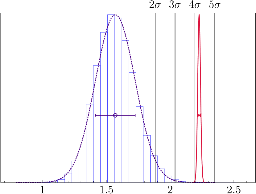
(a) Exclusive $|V_{cb}|$

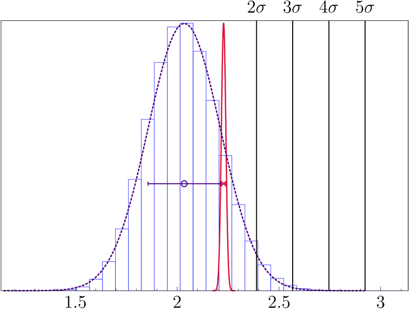
(b) Inclusive $|V_{cb}|$

Figure 3: $|\varepsilon_{K}|$ with (3(a)) exclusive $|V_{cb}|$ (left) and (3(b)) inclusive $|V_{cb}|$ (right) in units of $1.0\times 10^{-3}$.

Our results for $|\varepsilon_{K}|$ are summarized in Table 5. Here, the superscript ${}^{\text{SM}}$ means that it is obtained directly from the standard model, the subscript ${}_{\text{excl}}$ (${}_{\text{incl}}$) means that it is obtained using exclusive (inclusive) $|V_{cb}|$, and the superscript ${}^{\text{Exp}}$ represents the experimental value. Results in Table 5 (5(a)) are obtained using the RBC-UKQCD estimate for $\xi_{\text{LD}}$ and those in Table 5 (5(b)) are obtained using the BGI estimate for $\xi_{\text{LD}}$. In Table 5 (5(a)), we find that the theoretical evaluation of $|\varepsilon_{K}|$ with lattice QCD inputs (with exclusive $|V_{cb}|$) $|\varepsilon_{K}|^{\text{SM}}_{\text{excl}}$ has $4.2\sigma$ tension with the experimental result $|\varepsilon_{K}|^{\text{Exp}}$, while there is no tension with inclusive $|V_{cb}|$ (heavy quark expansion with QCD sum rules).

parameter	method	value
$|\varepsilon_{K}|^{\text{SM}}_{\text{excl}}$	exclusive $|V_{cb}|$	$1.570\pm 0.156$
$|\varepsilon_{K}|^{\text{SM}}_{\text{incl}}$	inclusive $|V_{cb}|$	$2.035\pm 0.178$
$|\varepsilon_{K}|^{\text{Exp}}$	experiment	$2.228\pm 0.011$

(a) RBC-UKQCD estimate for $\xi_{\text{LD}}$

parameter	method	value
$|\varepsilon_{K}|^{\text{SM}}_{\text{excl}}$	exclusive $|V_{cb}|$	$1.615\pm 0.158$
$|\varepsilon_{K}|^{\text{SM}}_{\text{incl}}$	inclusive $|V_{cb}|$	$2.079\pm 0.178$
$|\varepsilon_{K}|^{\text{Exp}}$	experiment	$2.228\pm 0.011$

(b) BGI estimate for $\xi_{\text{LD}}$

Table 5: $|\varepsilon_{K}|$ in units of $1.0\times 10^{-3}$.

In Fig. 4 (4(a)), we plot the $\Delta\varepsilon_{K}\equiv|\varepsilon_{K}|^{\text{Exp}}-|\varepsilon_{K}|^{\text{SM}}_{\text{excl}}$ in units of $\sigma$ (the total error) as a function of time starting from 2012. In 2012, $\Delta\varepsilon_{K}$ was $2.5\sigma$, but now it is $4.2\sigma$. In Fig. 4 (4(b)), we plot the history of the average $\Delta\varepsilon_{K}$ and the error $\sigma_{\Delta\varepsilon_{K}}$. We find that the average has increased with some fluctuations by 27% during the period of 2012-2018, and its error has decreased monotonically by 25% in the same period.

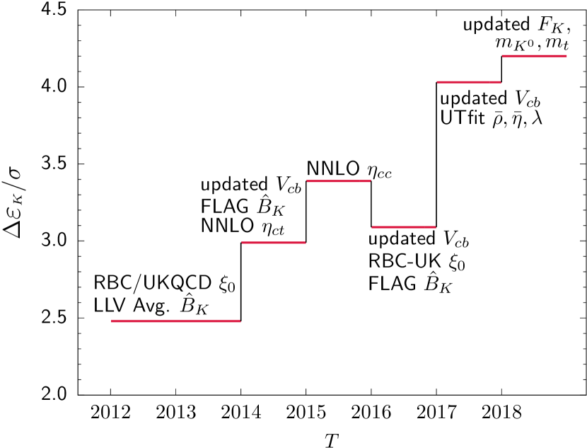
(a) Time evolution of $\Delta\varepsilon_{K}/\sigma$

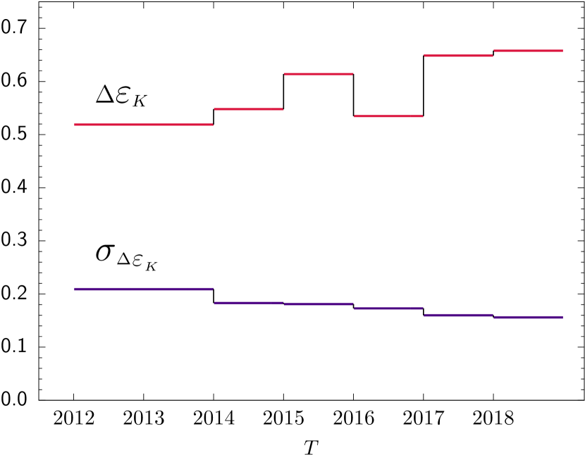
(b) Time evolution of the average and error of $\Delta\varepsilon_{K}$

Figure 4: Time history of (4(a)) $\Delta\varepsilon_{K}/\sigma$, and (4(b)) $\Delta\varepsilon_{K}$ and $\sigma_{\Delta\varepsilon_{K}}$.

In Table 6 (6(a)), we present the error budget for $|\varepsilon_{K}|^{\text{SM}}_{\text{excl}}$. Here, we find that the largest error comes from $|V_{cb}|$. Hence, it is essential to reduce the error in $|V_{cb}|$ significantly.

source	error (%)	memo
$|V_{cb}|$	31.4	ex-combined
$\bar{\eta}$	26.8	AOF
$\eta_{ct}$	21.5	$c-t$ Box
$\eta_{cc}$	9.1	$c-c$ Box
$\vdots$	$\vdots$	$\vdots$

(a) Error budget for $|\varepsilon_{K}|^{\text{SM}}_{\text{excl}}$

year	Inclusive $|V_{cb}|$	Exclusive $|V_{cb}|$
2015	$0.33\sigma$	$3.4\sigma$
2018	$1.1\sigma$	$4.2\sigma$

(b) Results for $\Delta\varepsilon_{K}$.

Table 6: Error budget for $|\varepsilon_{K}|^{\text{SM}}_{\text{excl}}$ and history of $\Delta\varepsilon_{K}$

In Table 6 (6(b)), we present how the values of $\Delta\varepsilon_{K}$ have changed from 2015 [3] to 2018 [1]. Here, we find that the positive shift of $\Delta\varepsilon_{K}$ is about the same for the inclusive and exclusive $|V_{cb}|$. This reflects the changes in other parameters since 2015.

- [1] J. A. Bailey, S. Lee, W. Lee, J. Leem, and S. Park 1808.09657.
- [2] Y.-C. Jang, W. Lee, S. Lee, and J. Leem EPJ Web Conf. 175 (2018) 14015, [1710.06614].
- [3] J. A. Bailey, Y.-C. Jang, W. Lee, and S. Park Phys. Rev. D92 (2015), no. 3 034510, [1503.05388].
- [4] J. A. Bailey, Y.-C. Jang, W. Lee, and S. Park PoS LATTICE2015 (2015) 348, [1511.00969].
- [5] Y. Amhis et al. Eur. Phys. J. C77 (2017), no. 12 895, [1612.07233].
- [6] J. A. Bailey, A. Bazavov, C. Bernard, et al. Phys.Rev. D89 (2014) 114504, [1403.0635].
- [7] J. A. Bailey et al. Phys. Rev. D92 (2015), no. 3 034506, [1503.07237].
- [8] W. Detmold, C. Lehner, and S. Meinel Phys. Rev. D92 (2015), no. 3 034503, [1503.01421].
- [9] Z. Bai et al. Phys. Rev. Lett. 115 (2015), no. 21 212001, [1505.07863].
- [10] G. Colangelo, J. Gasser, and H. Leutwyler Nucl. Phys. B603 (2001) 125–179, [hep-ph/0103088].
- [11] R. Garcia-Martin, R. Kaminski, J. R. Pelaez, J. Ruiz de Elvira, and F. J. Yndurain Phys. Rev. D83 (2011) 074004, [1102.2183].
- [12] T. Wang. https://indico.fnal.gov/event/15949/session/3/contribution/150/material/slides/0.pdf .
- [13] T. Blum et al. Phys. Rev. D91 (2015), no. 7 074502, [1502.00263].
- [14] https://indico.mitp.uni-mainz.de/event/48/contribution/5/material/slides/0.pdf.
- [15] A. Bevan, M. Bona, M. Ciuchini, D. Derkach, E. Franco, et al. Nucl.Phys.Proc.Suppl. 241-242 (2013) 89–94.
- [16] J. Charles et al. Eur.Phys.J. C41 (2005) 1–131, [hep-ph/0406184]. updated results and plots available at: http://ckmfitter.in2p3.fr.
- [17] M. Bona et al. JHEP 10 (2006) 081, [hep-ph/0606167]. Standard Model fit results: Summer 2016 (ICHEP 2016): http://www.utfit.org.
- [18] C. Patrignani et al. Chin. Phys. C40 (2016), no. 10 100001. https://pdg.lbl.gov/ .
- [19] G. Martinelli et al. http://www.utfit.org/UTfit/, 2017.
- [20] A. J. Buras and D. Guadagnoli Phys.Rev. D78 (2008) 033005, [0805.3887].
- [21] J. Brod and M. Gorbahn Phys.Rev. D82 (2010) 094026, [1007.0684].
- [22] S. Aoki et al. Eur. Phys. J. C77 (2017), no. 2 112, [1607.00299].
- [23] S. Durr et al. Phys. Lett. B705 (2011) 477–481, [1106.3230].
- [24] J. Laiho and R. S. Van de Water PoS LATTICE2011 (2011) 293, [1112.4861].
- [25] T. Blum et al. Phys. Rev. D93 (2016), no. 7 074505, [1411.7017].
- [26] B. J. Choi et al. Phys. Rev. D93 (2016), no. 1 014511, [1509.00592].
- [27] B. Chakraborty, C. T. H. Davies, B. Galloway, P. Knecht, J. Koponen, G. C. Donald, R. J. Dowdall, G. P. Lepage, and C. McNeile Phys. Rev. D91 (2015), no. 5 054508, [1408.4169].
- [28] N. Christ, T. Izubuchi, C. Sachrajda, A. Soni, and J. Yu Phys.Rev. D88 (2013), no. 1 014508, [1212.5931].
- [29] Z. Bai, N. Christ, T. Izubuchi, C. Sachrajda, A. Soni, et al. Phys.Rev.Lett. 113 (2014), no. 11 112003, [1406.0916].
- [30] N. H. Christ, X. Feng, G. Martinelli, and C. T. Sachrajda Phys. Rev. D91 (2015), no. 11 114510, [1504.01170].
- [31] N. H. Christ and Z. Bai PoS LATTICE2015 (2016) 342.
- [32] Z. Bai PoS LATTICE2016 (2017) 309, [1611.06601].
- [33] A. J. Buras, D. Guadagnoli, and G. Isidori Phys.Lett. B688 (2010) 309–313, [1002.3612].
- [34] N. Christ, T. Izubuchi, C. T. Sachrajda, A. Soni, and J. Yu PoS LATTICE2013 (2014) 397, [1402.2577].