Objective Bayesian Comparison of Order-Constrained Models in Contingency Tables

Abstract

In social and biomedical sciences testing in contingency tables often involves order restrictions on cell-probabilities parameters. We develop objective Bayes methods for order-constrained testing and model comparison when observations arise under product binomial or multinomial sampling. Specifically, we consider tests for monotone order of the parameters against equality of all parameters. Our strategy combines in a unified way both the intrinsic prior methodology and the encompassing prior approach in order to compute Bayes factors and posterior model probabilities. Performance of our method is evaluated on several simulation studies and real datasets.

Keywords: Bayes factor; contingency table; encompassing prior; intrinsic prior; order constraint; product binomial model

1 Introduction

Taking into account the ordering of categories in the analysis of two-way contingency tables may lead to improvements both in terms of power and model parsimony; see (Agresti & Coull, 2002). Often ordered categories can be naturally associated with inequality constraints among cell-probabilities, leading to substantial improvements over models which ignore the ordinal information.

Agresti & Coull (2002) provide an extensive survey of the analysis of contingency tables under inequality constraints from a frequentist perspective.

Over the years a growing dissatisfaction has emerged among statisticians over conventional measures of evidence such as $p$-values, as dramatically exemplified in Johnson et al. (2017) with special reference to psychological studies. In parallel Bayesian methods for hypotheses testing have become increasingly popular among practitioners; see again Wagenmakers (2007) with reference to Psychology where the issue of replication studies is especially critical.

In particular the Bayes Factor (Kass & Raftery (1995)) has emerged as a powerful tool for testing hypotheses (not necessarily nested) and model comparison. Additionally, if supplemented with prior model probabilities it leads to a full posterior distribution on the set of models under consideration, which entirely summarizes inference; see O’Hagan & Forster (2004), ch 7. This is a rich and informative output which provides an appreciation of the strengths of the various models, as well as of the associated uncertainty.

Bayesian testing for contingency tables dates back to the works of Good and co-authors, e.g. Good (1967); Crook & Good (1980); Good & Crook (1987), and was mostly focused on testing independence against an unrestricted hypothesis. The latter problem was approached from an objective Bayes perspective in Casella & Moreno (2009), while more specialized settings were discussed in Consonni & La Rocca (2008); Iliopoulos et al. (2009); Consonni et al. (2011). Testing of inequality-constrained hypotheses were initially dealt with in a series of papers with a focus on psychology studies; see for instance the review article Hoijtink (2013). Further analyses were presented Bartolucci et al. (2012) and Kateri & Agresti (2013).

All the previous papers relied on some form of subjectively specified (possibly weakly informative) priors. Over the years however the objective Bayes method has emerged as a powerful tool both for inference (Berger, 2006) and model choice (Pericchi, 2005; Consonni et al., 2018) where the prior is determined by formal rules which are model-dependent but otherwise are free form subjective elicitation. This turns out to be especially advantageous in model comparison, where the influence of the prior distribution is notoriously pervasive and persistent even with increasing sample size. This paper presents an objective Bayes methodology for the comparison of models for contingency tables specified by inequality constraints. In particular we follow an intrinsic prior approach (Berger & Pericchi, 1996; Moreno, 1997; Pérez & Berger, 2002), coupled with an encompassing prior approach, as we detail in the paper.

Specifically, we consider two scenarios. The first one concerns a collection of independent binary responses over $r$-ordered levels of a factor/predictor, so that the underlying sampling model is product binomial. Interest centers on testing the equality of the probabilities of success against a monotone ordering. We focus on binary responses for simplicity of exposition, although our methods could be conceptually extended to situations with polytomous responses (product multinomial model). In the second scenario we assume a joint multinomial model for the collection of cell frequencies, and test independence of rows and columns against inequality-constrained hypotheses on sets of cell probabilities, or functions thereof such as suitable odds-ratios.

The paper is organized as follows. Section 2 presents the product binomial model focusing on the comparison between the null model of equal probabilities and the full model; it also discusses conventional and intrinsic priors for this problem. Section 3 is devoted to the comparison of constrained product binomial models and contains the main contribution of the paper, named intrinsic-encompassing approach. Section 4 implements our procedure on the multinomial model. Section 5 presents some simulations and real applications in medical and psychological studies. Finally Section 6 offers some points for discussion.

2 Hypothesis testing in the product binomial model

2.1 Notation and likelihood

Let $U$ be a binary response variable, and $Z$ a factor having $r$ ordered levels, $z_{i}$, $i=1,\ldots,r$. Let $\pi_{i}=\mathrm{Pr}\{U=1|Z=z_{i},\pi_{i}\}$ be the probability of a success at level $Z=z_{i}$, $i=1,\ldots,r$. If a random sample of $n_{i}$ responses at level $z_{i}$ is available, denote with $Y_{i}$ the number of successes out of the $n_{i}$ trials. Then, conditionally on $\pi_{i}$, $Y_{i}$ is $\mbox{Binomial}(n_{i},\pi_{i})$. If the $Y_{i}$’s are assumed to be independent, their sampling distribution - and by extension that of the allied $r\times 2$ contingency table containing the frequencies $\{(Y_{i},n_{i}-Y_{i}),\,i=1,\ldots,r\}$ - is product Binomial.

We now discuss briefly, for completeness and for later use the standard setting, wherein interest centers on testing the null model (hypothesis) of equality of success probabilities across levels of $Z$

$$M_{0}:\pi_{1}=\pi_{2}=\ldots=\pi_{r}=\pi^{*}$$ (1)

against the encompassing model

$$M_{e}:(\pi_{i},i=1,\ldots,r)\in\{[0,1]^{r}\setminus\{\pi_{1}=\ldots=\pi_{r}\}\}.$$ (2)

Notice that $M_{e}$ imposes no restriction on the collection of probabilities $\{\pi_{i}\}$ save for barring the possibility of complete equality. For this reason $M_{e}$ could also be named unconstrained; however we prefer the term encompassing for reasons that will become clear later on.

Let $\bm{y}=(y_{i},i=1,\ldots,r)$, and set $\bm{\pi}=(\pi_{1},\ldots,\pi_{r})$. The sampling distribution of $\bm{Y}$ for given $(n_{i},i=1,\ldots,r)$ under $M_{0}$, respectively $M_{e}$, is

$$f(\bm{y}|\pi^{*},M_{0})=\prod_{i=1}^{r}\binom{n_{i}}{y_{i}}{\pi^{*}}^{y_{i}}(1-\pi^{*})^{n_{i}-y_{i}}=K(\bm{n},\bm{y})\left\{{\pi^{*}}^{s_{y}}(1-\pi^{*})^{n-s_{y}}\right\}$$ (3)

$$f(\bm{y}|\bm{\pi},M_{e})=\prod_{i=1}^{r}\binom{n_{i}}{y_{i}}\pi_{i}^{y_{i}}(1-\pi_{i})^{n_{i}-y_{i}}=K(\bm{n},\bm{y})\left\{\prod_{i=1}^{r}\pi_{i}^{y_{i}}(1-\pi_{i})^{n_{i}-y_{i}}\right\}$$ (4)

where $K(\bm{n},\bm{y})=\prod_{i=1}^{r}\binom{n_{i}}{y_{i}}$, $n=\sum_{i=1}^{r}n_{i1}$, $s_{y}=\sum_{i=1}^{r}y_{i}$ and $\bm{n}=(n_{1},\ldots,n_{r})$.

2.2 Conventional priors

Denote with $p^{N}(\bm{\pi}|M_{e})$ an objective prior for $\bm{\pi}$ under model $M_{e}$. Typically, this will be a reference (Bernardo, 1979), or default, prior used for estimation purposes. The superscript “$N$” stands for noninformative. A natural family for such a prior is a product of Beta distributions

$$p^{N}(\bm{\pi}|M_{e})=\prod_{i=1}^{r}Beta(\pi_{i}|\alpha_{i1},\alpha_{i2}).$$

Now let $\pi^{*}$ be the success probability common to all levels under $M_{0}$. A default prior is

$$p^{N}(\pi^{*}|M_{0})=Beta(\pi^{*}|\alpha_{01},\alpha_{02}).$$

A standard choice might be $\alpha_{i1}=\alpha_{i2}=1$, for $i=1,\ldots,r$, and $\alpha_{01}=\alpha_{02}=1$, corresponding to a uniform prior; alternatively one could choose the value 1/2 as in the Jeffreys prior.

The marginal likelihood under each of the two models is given by

$$m^{N}(\bm{y}|M_{0})=\int_{0}^{1}f(\bm{y}|\pi^{*},M_{0})p^{N}(\pi^{*}|M_{0})d\pi^{*}$$ (5)

$$= K(\bm{n},\bm{y})\frac{B(\alpha_{01}+s_{y},\alpha_{02}+n-s_{y})}{B(\alpha_{01},\alpha_{02})}$$

and

$$m^{N}(\bm{y}|M_{e})=\int_{0}^{1}f(\bm{y}|\bm{\pi},M_{e})p^{N}(\bm{\pi}|M_{e})d\bm{\pi}$$ (6)

$$= K(\bm{n},\bm{y})\prod_{i=1}^{r}\frac{B(\alpha_{i1}+y_{i},\alpha_{i2}+n_{i}-y_{i})}{B(\alpha_{i1},\alpha_{i2})}.$$

They are subsequently employed to produce the Bayes factor (BF) of $M_{e}$ against $M_{0}$ which is given by

$$BF_{e0}^{N}(\bm{y})=\frac{m^{N}(\bm{y}|M_{e})}{m^{N}(\bm{y}|M_{0})},$$ (7)

where the superscript $N$ is used to remind us that the BF is computed using the default priors, and to distinguish it from an alternative BF we shall employ later on.

2.3 Intrinsic priors

It is by now an established fact within the Bayesian community that objective priors, which have been designed for estimation purposes conditionally on a given model, are largely inadequate for model comparison or hypotheses testing; see Pericchi (2005) and Consonni et al. (2018). This is patently evident when the objective prior under any of the two models is improper, because the presence of an arbitrary normalizing constant in the prior transfers to the marginal likelihood and consequently makes the $BF^{N}$ meaningless. However the rationale for not using conventional objective priors for testing holds also when the prior under each of the two models is proper, as in our case. The reason for this is that $p^{N}(\bm{\pi}|M_{e})$ is not compatible with $p^{N}(\pi|M_{0})$, i.e. it is not chosen in view of the comparison with model $M_{0}$. For more information on the issue of compatibility of priors for model selection see Consonni & Veronese (2008).

In particular, a conventional objective prior $p^{N}(\bm{\pi}|M_{e})$ is generally diffuse, and thus gives relatively little weight to parameter values close to the subspace characterizing $M_{0}$. Consequently, there is an evidence bias in favor of $M_{0}$ (unless the data are vastly against $M_{0}$, which rarely happens for moderate sample sizes). Informally, one can say that $p^{N}(\cdot|M_{e})$ “wastes” away probability mass in parameter areas too remote from the null. To overcome this difficulty, one ought to modify $p^{N}(\cdot|M_{e})$ so that it reallocates more probability mass toward the null subspace, an idea already advocated in Jeffreys (1961, Chapter 3). This of course has a negative side effect, at least for moderate sample sizes, because it will diminish evidence in favor of $M_{e}$ when the parameter values generating the data are truly away from the null. However this is a price worth paying, as explicated in Consonni et al. (2013), to whom we refer the reader for further considerations about issues discussed in this subsection.

We now describe a strategy to implement the above program based on the notion of intrinsic priors, which were introduced in objective hypothesis testing to deal in a sensible way with improper default priors; see Berger & Pericchi (1996) and Moreno (1997). However the scope of the intrinsic prior approach is much wider, because it represents a general methodology for Bayesian model choice, and can be used in any circumstance, and so also when the starting default priors are proper, as in our case. The reason why intrinsic priors are especially effective is easily seen when comparing two nested models, such as $M_{0}$ and $M_{e}$ in Section 2. The basic idea is to introduce a set of imaginary observations, i.e. auxiliary random variables, to “train” the default prior $p^{N}(\cdot|M_{e})$ so that its diffuseness is reduced by shifting some probability mass toward the null subspace characterizing $M_{0}$. Let us see how we can achieve this goal in the setup of a product binomial model. Let $\bm{x}=(x_{i},i=1,\ldots,r)$ be imaginary observations, with $x_{i}$ representing the number of successes out of $t_{i}$ trials, and set $\bm{t}=(t_{1},\ldots,t_{r})$. The intrinsic prior under model $M_{e}$ for the comparison with model $M_{0}$ is defined as

$$p^{I}(\bm{\pi}|\bm{t},M_{e})=\sum_{\bm{x}}p^{N}(\bm{\pi}|\bm{t},\bm{x},M_{e})m^{N}(\bm{x}|\bm{t},M_{0}),$$ (8)

where $p^{N}(\bm{\pi}|\bm{t},\bm{x},M_{e})\propto p^{N}(\bm{\pi}|M_{e})f(\bm{x}|\bm{t},\bm{\pi},M_{e})$, so that

$$p^{N}(\bm{\pi}|\bm{t},\bm{x},M_{e})=\prod_{i=1}^{r}Beta(\pi_{i}|\alpha_{i1}+x_{i};\alpha_{i2}+t_{i}-x_{i}).$$ (9)

On the other hand

$$m^{N}(\bm{x}|\bm{t},M_{0})=K(\bm{t},\bm{x})\frac{B(\alpha_{01}+s_{x},\alpha_{02}+t-s_{x})}{B(\alpha_{01},\alpha_{02})}$$

is the marginal distribution of $\bm{X}$ under model $M_{0}$ with prior $p^{N}(\cdot|M_{0})$ which can be seen to be the analogue of (5) upon replacing $\bm{y}$ with $\bm{x}$ and $\bm{n}$ with $\bm{t}$, so that $s_{x}=\sum_{i=1}^{r}x_{i}$ and $t=\sum_{i=1}^{r}t_{i}$.

Remarks

• The intrinsic prior is a mixture of “pseudo-posteriors” $p^{N}(\bm{\pi}|\bm{x},M_{e})$ with respect to the mixing distribution $m^{N}(\bm{x}|M_{0})$. As a consequence, the individual $\pi_{i}$’s, which were independent under $p^{N}(\cdot|M_{e})$ are no longer so under $p^{I}(\cdot|M_{e})$.

• It can be checked that if the training sample size for row $i$, $t_{i}$ is zero, i.e. if no intrinsic procedure is applied, then marginally $p^{I}(\pi_{i}\,|\,t_{i}=0,M_{e})=p^{N}(\pi_{i})$, i.e. the intrinsic prior reduces to the initial prior which is recovered as a special case. On the other hand, as each of the $t_{i}$ increases, $p^{I}(\bm{\pi}|\bm{t},M_{e})$ will transfer more mass to the one-dimensional subspace $\pi_{1}=\pi_{2}=\dots,\pi_{r}$, so that in the limit $p^{I}(\bm{\pi}|\bm{t},M_{e})$ will degenerate to a uniform distribution on that subspace: see Fig. 1 for an illustration of this phenomenon. As a consequence the intrinsic marginal data distribution $m^{I}(\bm{y}|\bm{t},M_{e})=\int f(\bm{y}|\bm{\pi},M_{e})p^{I}(\bm{\pi}|\bm{t},M_{e})$ will tend to $m^{N}(\bm{y}|M_{0})$, and the corresponding BF will converge to one. One can thus see that the choice of the $t_{i}$’s is quite important in comparing the two models because it regulates the amount of concentration of the intrinsic prior around the null subspace. To circumvent this difficulty, it is customary to set $t_{i}$ equal to a minimal training sample size (Berger & Pericchi, 2004) which guarantees that the posterior is proper. In our setup however, because our starting default priors are already proper under each of the two models, the notion of minimal training sample size becomes useless. Accordingly, we will let each $t_{i}$ range over the integers in the set $\{0,1,\ldots,n_{i}\}$, thus effectively performing a sensitivity analysis. This means that if the results do not change appreciably as $t_{i}$ varies, then our inferential conclusion is robust.

• The intrinsic prior in (8) is a special case of the expected posterior prior introduced in Pérez & Berger (2002) for the comparison of several models $M_{k}$ each equipped with a default prior $p^{N}(\cdot|M_{k})$. In that case the intrinsic prior under $M_{k}$ is as in (8) with the mixing distribution $m^{N}(\cdot|M_{0})$ replaced by a more general measure $m^{*}(\cdot)$, which however must be the same for all models.

• A very simple expression of the intrinsic prior can be written under the constrained hypothesis, due to the exchangeability property, when the sizes of the training samples are equal $t_{1}=t_{2}=\ldots=t_{r}$ (see the Supplementary Material).

An illustration of the behavior of the intrinsic prior in the simple case of $r=2$ is provided in Figure 1 for different training sample sizes $\bar{t}=t_{1}=t_{2}$, and with all hyperparameters $\alpha$’s set to 1. Notice that as $\bar{t}$ increases, the intrinsic prior progressively concentrates around the line $\pi_{1}=\pi_{2}$.

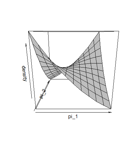
(a) $\bar{t}=3$

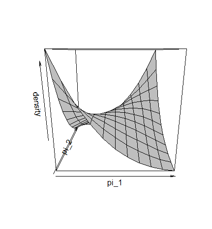
(b) $\bar{t}=5$

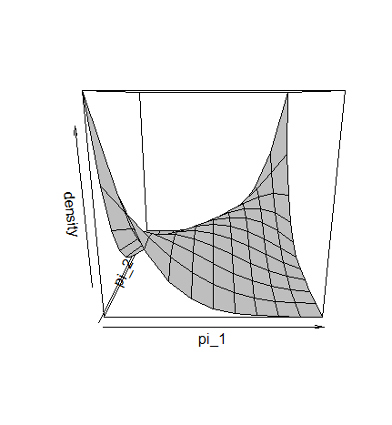
(c) $\bar{t}=10$

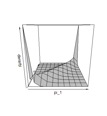
(d) $\bar{t}=50$

Figure 1: Intrinsic prior for different values of the training sample size $\bar{t}$.

3 Comparison of constrained product binomial models

Agresti & Coull (2002, Table 1) discuss a clinical trial applied to patients who experienced trauma due to subarachnoid hemorrhage. Factor $Z$ has four levels, corresponding to a placebo followed by three increasing doses of a medication. The outcome variable has five levels (“Death”, “Vegetative state”, “Major disability”,“Minor disability ”,“Good recovery”) but for illustration purposes it has been collapsed to a binary variable, with categories “Death” and “Not Death”. The resulting $4\times 2$ contingency table is reported in Table 1.

Table 1: Responses from a clinical trial comparing four treatments on patients who experienced trauma due to subarachnoid hemorrhage

Treatment	Outcome
	Death	Not Death
Placebo	59	151
Low dose	48	142
Medium dose	44	163
High dose	43	152

It is expected that a more favorable outcome tends to occur as the dose increases. Taking this information into account, the null model $M_{0}$ in (1) is tested against the model based on an ordered restriction of the probabilities of Death $\pi_{i}$:

$$M_{c}:\pi_{1}>\pi_{2}>\ldots>\pi_{r}.$$ (10)

In the sequel $M_{c}$ will denote a generic constrained model containing inequalities constraints such as those in (10). More general types of constrained models could be envisaged, such as those containing a mixture of equality and inequality constraints; see for instance Mulder (2014).

To perform this comparison using the Bayes factor we require a prior on the parameter space under model $M_{c}$. This can be achieved using an encompassing prior approach (Klugkist & Hoijtink, 2007), which we now briefly summarize. Let $M_{c}$ be a constrained model whose parameter space $\bm{\Theta_{c}}$ is specified by means of inequalities on the components of $\bm{\theta}\in\bm{\Theta}$, with $\bm{\Theta}$ being the unconstrained parameter space of the encompassing model $M_{e}$. Let $p(\bm{\theta}|M_{e})$ be a (proper) prior under $M_{e}$. A natural way to construct a prior under $M_{c}$ is by truncation, namely $p(\bm{\theta}|M_{c})\propto p(\bm{\theta}|M_{e})\bm{1}_{\bm{\Theta}_{c}}(\bm{\theta})$, where $\bm{1}_{A}(\cdot)$ is the indicator function of the set $A$. A straightforward calculation (Klugkist & Hoijtink, 2007) shows that, for fixed data $\bm{y}$, the Bayes factor of $M_{c}$ against $M_{e}$, is given by the ratio ${\mathrm{Pr}\{\bm{\theta}\in\bm{\Theta}_{c}|\bm{y},M_{e}\}}/{\mathrm{Pr}\{\bm{\theta}\in\bm{\Theta}_{c}|M_{e}\}}$. Note that both the prior and the posterior probability of the set $\bm{\Theta}_{c}$ are evaluated under the unconstrained model $M_{e}$. Wetzels et al. (2010) provide further comments on the encompassing prior approach.

Having specified the theoretical framework we work with, our strategy to construct an objective Bayes factor of model $M_{c}$, specified by the constrained parameter space $\bm{\Theta}_{c}$, as for instance in (10), against $M_{0}$ can be outlined as follows:

• start with an objective prior $p^{N}(\bm{\pi}|M_{e})$, which we assume to be proper;

• for given training sample sizes $\bm{t}$, construct the intrinsic prior $p^{I}(\bm{\pi}|\bm{t},M_{e})$ tailored to the comparison of $M_{e}$ against $M_{0}$ as in (8), and derive the BF based on the intrinsic prior (which we label as $BF^{I}$)

  $$BF^{I}_{e0}(\bm{y}|\bm{t})=\frac{m^{I}(\bm{y}|\bm{t},M_{e})}{m^{N}(\bm{y}|M_{0})},$$ (11)

  where $m^{I}(\bm{y}|\bm{t},M_{e})=\int f(\bm{y}|\bm{\pi},M_{e})p^{I}(\bm{\pi}|\bm{t},M_{e})d\bm{\pi}$;

• compute

  $$BF^{I}_{ce}(\bm{y}|\bm{t})=\frac{\mathrm{Pr}^{I}\{\bm{\pi}\in\bm{\Theta}_{c}|\bm{t},\bm{y},M_{e}\}}{\mathrm{Pr}^{I}\{\bm{\pi}\in\bm{\Theta}_{c}|\bm{t},M_{e}\}};$$ (12)

• finally derive

  $$BF^{I}_{c0}(\bm{y}|\bm{t})=BF^{I}_{ce}(\bm{y}|\bm{t})\times BF^{I}_{e0}(\bm{y}|\bm{t}).$$ (13)

The above procedure, which we name intrinsic-encompassing, was first presented in Consonni & Paroli (2017) with regard to the comparison of constrained ANOVA models. There is however a significant difference. In that setting the starting default priors were improper, so that in particular the intrinsic prior under $M_{e}$ was also improper; accordingly the procedure had to be based on the conditional intrinsic prior (which is always proper), rather than the actual intrinsic prior, as in our current setup. The main advantage of the intrinsic-encompassing approach is contained in formula (13). It can be seen that the computation of $BF^{I}_{c0}(\bm{y}|\bm{t})$ is decoupled into two parts: i) one involving the computation of the “standard” Bayes factor $BF^{I}_{e0}(\bm{y}|\bm{t})$, and ii) one involving the evaluation of two probabilities of the set $\bm{\Theta}_{c}$. While the latter formally requires integrating over $\bm{\Theta}_{c}$, a simulation-based approximation is typically available based on draws from the intrinsic prior, respectively posterior, under the unconstrained model $M_{e}$.

Assuming that the true model belongs to a finite space of (not necessarily nested) constrained models $\{M_{c}:c\in{\cal C}\}$, the above procedure can be used to obtain the posterior distribution on model space, provided one can identify a single null model $M_{0}$ which is nested into any model under consideration. In that case one gets

$$\mathrm{Pr}^{I}(M_{c}|\bm{t},\bm{y})=\frac{BF^{I}_{c0}(\bm{y}|\bm{t})}{1+(\sum_{c^{\prime}\in{\cal C}}BF^{I}_{c^{\prime}0}(\bm{y}|\bm{t})P_{c^{\prime}0})},\,c\in{\cal C},$$ (14)

where $P_{c0}=\mathrm{Pr}(M_{c})/\mathrm{Pr}(M_{0})$ is the prior odds of model $M_{c}$ against model $M_{0}$. Notice that the calculation leading to (14) is coherent because the marginal distribution of the data under $M_{0}$, $m^{N}(\bm{y}|M_{0})$, is the same under any Bayes factor involved in (14). This means in particular that the BF for the comparison of models $M_{c}$ and $M_{c^{\prime}}$ is computable as $BF^{I}_{cc^{\prime}}(\bm{y}|\bm{t})=BF^{I}_{c0}(\bm{y}|\bm{t})/BF^{I}_{c^{\prime}0}(\bm{y}|\bm{t})$. It is important to realize that the posterior probability of model $M_{c}$ will depend not only on the fit to the observations but also to the model complexity. This is because the Bayes factor incorporates an automatic Ockham’s razor (Jefferys & Berger, 1992), whereby more complex models are implicitly discounted. Interestingly, this penalization applies not only to the standard comparison of two models having different dimensionality (number of parameters) but also to models having the same dimension wherein one has a smaller parameter space. In particular our approach allows to meaningfully compare an inequality constrained model with an unconstrained model, so that the former may receive a higher posterior probability than the latter as some examples below will clarify.

3.1 BF of the encompassing model against the null model

In this subsection we detail calculations to obtain (11) in our setting.

The summations involved may cause computational problems when the number of groups $r$ and the dimensions of the training sample $t_{i}$ are large because the number of their terms becomes prohibitively large. This difficulty can be effectively overcome by means of Monte Carlo sum as described in Casella & Moreno (2005) and Consonni et al. (2011).

On the other hand (Pérez & Berger, 2002, (4.2)) showed that $BF^{I}_{e0}(\bm{y}|\bm{t})$ can be approximated using importance sampling as

$$\widehat{BF}^{I}_{e0}(\bm{y}|\bm{t})\simeq\frac{1}{S}\sum_{s=1}^{S}\frac{m^{N}(\bm{y}|\bm{t},\bm{x}^{(s)},M_{e})}{m^{N}(\bm{y}|\bm{t},\bm{x}^{(s)},M_{0})},$$ (15)

where $\bm{x}^{(s)}$, $s=1,\ldots,S$, are draws from the importance distribution $m^{N}(\bm{x}|\bm{t},\bm{y},M_{0})$. The analytical form of the terms appearing in (15) are specified below.

$$m^{N}(\bm{y}|\bm{t},\bm{x},M_{e})=K(\bm{n},\bm{y})\prod_{i=1}^{r}\frac{B(\alpha_{i1}+x_{i}+y_{i};\alpha_{i2}+(t_{i}-x_{i})+(n_{i}-y_{i}))}{B(\alpha_{i1}+x_{i};\alpha_{i2}+(t_{i}-x_{i}))},$$

$$m^{N}(\bm{y}|\bm{t},\bm{x},M_{0})=K(\bm{n},\bm{y})\frac{B(\alpha_{01}+s_{x}+s_{y};\alpha_{02}+(t-s_{x})+(n-s_{y}))}{B(\alpha_{01}+s_{x};\alpha_{02}+(t-s_{x}))}.$$

Finally the importance distribution is given by

$$m^{N}(\bm{x}|\bm{t},\bm{y},M_{0})=K(\bm{t},\bm{x})\frac{B(\alpha_{01}+s_{x}+s_{y};\alpha_{02}+(t-s_{x})+(n-s_{y}))}{B(\alpha_{01}+s_{y};\alpha_{02}+(n-s_{y}))}.$$ (16)

To sample from (16) one can proceed as follows:

• sample $\pi^{(s)}$ from the posterior distribution $p^{N}(\bm{\pi}|\bm{y},M_{0})$

  $$\pi^{(s)}|\bm{y},M_{0}\sim Beta(\alpha_{01}+s_{y};\alpha_{02}+(n-s_{y})),$$

• sample each element of $\bm{x}^{(s)}$ independently

  $$x_{i}^{(s)}|t_{i},\pi^{(s)},M_{0}\sim Bin(x_{i}|t_{i},\pi^{(s)}),\,i=1,\ldots,r.$$

3.2 BF of the constrained model against the encompassing model

The expression for $BF^{I}_{ce}(\bm{y}|\bm{t})$ in (12) is a ratio of probabilities for the same subspace $\bm{\Theta}_{c}$. The denominator involves the intrinsic prior, which is is given by

$$p^{I}(\bm{\pi}|\bm{t},M_{e})=\sum_{\bm{x}}\left\{\left[\prod_{i=1}^{r}Beta(\pi_{i}|\alpha_{i1}+x_{i};\alpha_{i2}+t_{i}-x_{i})\right]m^{N}(\bm{x}|\bm{t},H_{0})\right\}.$$ (17)

On the other hand, the numerator involves the intrinsic posterior distribution, whose density can be written as

$$p^{I}(\bm{\pi}|\bm{y},\bm{t},M_{e})$$ (18)

$$= \sum_{\bm{x}}\left\{\prod_{i=1}^{r}Beta(\pi_{i}|\alpha_{i1}+x_{i}+y_{i};\alpha_{i2}+(t_{i}-x_{i})+(n_{i}-y_{i}))\right\}m^{*}(\bm{x}|\bm{t},\bm{y}),$$

where

$$m^{*}(\bm{x}|\bm{t},\bm{y})=\frac{m^{N}(\bm{y}|\bm{x},\bm{t},M_{e})m^{N}(\bm{x}|\bm{t},M_{0})}{\sum_{\bm{x}}m^{N}(\bm{y}|\bm{x},\bm{t},M_{e})m^{N}(\bm{x}|\bm{t},M_{0})}.$$

We can write more compactly

$$m^{*}(\bm{x}|\bm{t},\bm{y})=\frac{H(\bm{x}|\bm{t},\bm{y})}{\sum_{\bm{x}}H(\bm{x}|\bm{t},\bm{y})},$$

where

$$H(\bm{x}|\bm{t},\bm{y}) = K(\bm{t},\bm{x})\left[\prod_{i=1}^{r}\frac{B(\alpha_{i1}+x_{i}+y_{i};\alpha_{i2}+(t_{i}-x_{i})+(n_{i}-y_{i}))}{B(\alpha_{i1}+x_{i},\alpha_{i2}+(t_{i}-x_{i}))}\right]$$ (19)

$$\times B(\alpha_{01}+s_{x},\alpha_{02}+t-s_{x}),$$

since the function $H(\bm{x}|\bm{t},\bm{y})$ will be used later on in our computations.

Both the intrinsic prior and posterior are discrete mixtures of product of Beta distributions with respect to the imaginary observations $\bm{x}$. In both cases the number of terms in the sum can be prohibitively large; additionally, for each fixed $\bm{x}$, integration over $\Theta_{c}$ is typically not analytically available. To address the above difficulties, we can use an importance sampling strategy, as for instance implemented in Casella & Moreno (2009) and Consonni et al. (2011) in the context of intrinsic priors involving discrete mixtures.

Consider first the evaluation of the denominator of $BF^{I}_{ce}$. We approximate the required probability by drawing $S$ independent and identically distributed samples from the intrinsic prior (17). The latter in turn can be regarded as the marginal distribution of $\bm{\pi}$, derived from the joint distribution

$$p(\bm{\pi},\pi,\bm{x})=p^{N}(\pi|M_{0})f(\bm{x}|\pi,\bm{t},M_{0})p^{N}(\bm{\pi}|\bm{t},\bm{x},M_{e}).$$

Each of these three components can be sampled iteratively, and in the end we retain only the $\bm{\pi}$-values (see Algorithm 1).

Consider now the numerator of $BF^{I}_{ce}$. Since it is not possible to sample exactly from the intrinsic posterior distribution, we rely on a Metropolis within Gibbs algorithm as in Algorithm 2.

Finally obtain

$$\widehat{BF}^{I}_{c,e}(\bm{y}|\bm{t})=\frac{\widehat{\mathrm{Pr}}^{I}\{\pi_{1}>\pi_{2}>\ldots>\pi_{r}|\bm{y},\bm{t},M_{e}\}}{\widehat{\mathrm{Pr}}^{I}\{\pi_{1}>\pi_{2}>\ldots>\pi_{r}|\bm{t},M_{e}\}}.$$

Algorithm 1 Approximation of the denominator of (12)

1:for $s=1,2,\ldots,S$ do

2:     sample $\pi^{(s)}$ from $p^{N}(\pi|M_{0})$: $\pi^{(s)}\sim Beta(\alpha_{01},\alpha_{02})$;

3:     sample independently each element $x_{i}$ of $\bm{x}^{(s)}$ from $f({x_{i}}|\pi^{(s)},{t_{i}},M_{0})$: $x_{i}^{(s)}|\pi^{(s)},t_{i},M_{0}\sim Bin(x_{i}|t_{i},\pi^{(s)})$;

4:     sample independently each element ${{\pi_{i}}^{(s)}}$ of $\bm{\pi}^{(s)}$ from the pseudo posterior $p^{N}({\pi_{i}}|{t_{i}},{x_{i}^{(s)}},M_{e})$: $\pi_{i}^{(s)}|{x_{i}}^{(s)},M_{e}\sim Beta(\pi_{i}|\alpha_{i1}+x_{i}^{(s)},\alpha_{i2}+t_{i}-x_{i}^{(s)})$;

5:end for

6:Approximate the probability as

$$\widehat{\mathrm{Pr}}^{I}\{\pi_{1}>\pi_{2}>\ldots>\pi_{r}|M_{e}\}\thickapprox\frac{1}{S}\sum_{s=1}^{S}\bm{1}_{\pi_{1}^{(s)}>\pi_{2}^{(s)}>\ldots>\pi_{r}^{(s)}}(\bm{\pi}^{(s)}).$$

Algorithm 2 Approximation of the numerator of (12)

1:estimate the probabilities $\pi_{i}$, $i=1,2,\ldots,r$ as

$$\widehat{\pi_{i}}=\frac{y_{i}+1}{s_{y}+r},\forall i=1,2,\ldots,r;$$

2:generate the imaginary training sample elements with this step of Metropolis:

3:sample the starting values $x_{i}^{(0)}\sim Bin(t_{i},\widehat{\pi_{i}})$, $\forall i=1,\ldots,r$, independently;

4:for $s=1,2,\ldots,S_{1}$ do

5:     generate $\bm{x}^{(s)}$ by sampling each component $x_{i}^{(s)}$ from the proposal $Bin(t_{i},\widehat{\pi_{i}})$, independently for $i=1,\ldots,r$, and accept it with probability:

$$\alpha\left(\bm{x}^{(s-1)};\bm{x}^{(s)}\right)=\min\left\{1;\frac{H(\bm{x}^{(s)}|\bm{t},\bm{y})\prod_{i=1}^{r}Bin({x}_{i1}^{(s-1)}|t_{i},\widehat{\pi_{i}})}{H(\bm{x}^{(s-1)}|\bm{t},\bm{y})\prod_{i=1}^{r}Bin({x}_{i1}^{(s)}|t_{i},\widehat{\pi_{i}})}\right\};$$

where $H(\bm{x}|\bm{t},\bm{y})$ is defined in (19).

6:end for

7:after a suitable number of burn-in iterations $S_{1}$, start sampling $\bm{\pi}^{(s)}$:

8:for $s=S_{1}+1,\ldots,S_{1}+S$ do

9:     repeat step (5) with the following addition: sample each component $\pi_{i}^{(s)}$ of $\bm{\pi}^{(s)}$ from $\pi_{i}^{(s)}|t_{i},{x}_{i1}^{(s)},M_{e}\sim Beta(\alpha_{i1}+x^{(s)}_{i1},\alpha_{i2}+t_{i}-x^{(s)}_{i1}),$ independently for $i=1,\ldots,r$;

10:end for

11:approximate the probability of the numerator of (12) as

$$\widehat{\mathrm{Pr}}^{I}\{\pi_{1}>\pi_{2}>\ldots>\pi_{r}|\bm{y},\bm{t},M_{e}\}\thickapprox\frac{1}{S}\sum_{s=S_{1}+1}^{S_{1}+S}\bm{1}_{\pi_{1}^{(s)}>\pi_{2}^{(s)}>\ldots>\pi_{r}^{(s)}}(\bm{\pi}^{(s)}).$$

4 Hypothesis testing in the multinomial model

In this section we extend the scope of our methodology to an $r\times c$ contingency table under a multinomial sampling model. Denote with $\bm{y}=\{y_{ij},i=1,\ldots,r,j=1,\ldots,c\}$, with $\sum_{i=1}^{r}\sum_{j=1}^{c}y_{ij}=n$ the cell frequencies. Under the encompassing model $M_{e}$ all cell probabilities are unconstrained, save for adding up to one, and we write $\bm{\pi}=\{\pi_{ij},i=1,\ldots,r,j=1,\ldots,c\}$ and $\sum_{i=1}^{r}\sum_{j=1}^{c}\pi_{ij}=1$. A default prior for $\bm{\pi}$ is Dirichlet with hyperparameters $\bm{\alpha}_{\pi}$ $p^{N}(\bm{\pi}|M_{e})=Di(\bm{\pi}|\bm{\alpha}_{\pi}).$ Typically $\bm{\alpha}_{\pi}$ has all its $rc$ elements equal to 1 (Uniform prior) or equal to $1/2$ (Jeffreys prior). For given $n$, the sampling distribution of $\bm{Y}$ under model $M_{e}$ is

$$f(\bm{y}|\bm{\pi},M_{e})=\binom{n}{\bm{y}}\prod_{i=1}^{r}\prod_{j=1}^{c}\pi_{ij}^{y_{ij}},$$ (20)

where $\binom{n}{\bm{y}}$ is the multinomial coefficient.

Let $\bm{\pi_{R}}$ and $\bm{\pi_{C}}$ be the vectors of row, respectively column, marginal probabilities, with $\sum_{i=1}^{r}\pi_{Ri}=1$ and $\sum_{j=1}^{c}\pi_{Cj}=1$. Denote the null model of independence by

$$M_{0}:\pi^{0}_{i,j}=\pi_{Ri}\cdot\pi_{Cj},\quad i=1,\ldots,r;\,j=1,\ldots,c$$ (21)

A default prior on $(\bm{\pi_{R}},\bm{\pi_{C}})$ is

$$p^{N}(\bm{\pi_{R}},\bm{\pi_{C}}|M_{0})=Di(\bm{\pi_{R}}|\bm{\alpha}_{\pi_{R}})\cdot Di(\bm{\pi_{C}}|\bm{\alpha}_{\pi_{C}}),$$

Typically both $\bm{\alpha}_{\pi_{R}}$ and $\bm{\alpha}_{\pi_{C}}$ have each all elements equal to 1 (Uniform prior) or equal to $1/2$ (Jeffreys prior). The likelihood function under $M_{0}$ is

$$f(\bm{y}|\bm{\pi_{R}},\bm{\pi_{C}},M_{0})=\binom{n}{\bm{y}}\left(\prod_{i=1}^{r}\pi_{Ri}^{y_{i+}}\right)\left(\prod_{j=1}^{c}\pi_{Cj}^{y_{+j}}\right),$$ (22)

where $y_{i+}=\sum_{j=1}^{c}y_{ij}$ and $y_{+j}=\sum_{i=1}^{r}y_{ij}$.

The marginal likelihood for the null model is given by

$$m^{N}(\bm{y}|M_{0})=\binom{n}{\bm{y}}\frac{B(\bm{\alpha}_{\pi_{R}}+\bm{y_{R+}})B(\bm{\alpha}_{\pi_{C}}+\bm{y_{+C}})}{B(\bm{\alpha}_{\pi_{R}})B(\bm{\alpha}_{{\pi_{C}}})}$$ (23)

with $\bm{y_{R+}}=(y_{i+},i=1,\ldots,r)$ and $\bm{y_{+C}}=(y_{+j},j=1,\ldots,c)$, and where $B$ stands for the multivariate Beta function.

In the multinomial model the constrained model $M_{c}$ is often stated in terms of inequality constraints between sets of cell probabilities or functions of cell probabilities like odds ratios; for more details see Agresti & Coull (2002).

4.1 Intrinsic priors

Let $\bm{x}=(x_{ij},i=1,\ldots,r,j=1,\ldots,c)$ be a matrix of imaginary observations, with $\sum_{i=1}^{r}\sum_{j=1}^{c}x_{ij}=t$. The intrinsic prior under model $M_{e}$ for the comparison with model $M_{0}$ is given by

$$p^{I}(\bm{\pi}|t,M_{e})=\sum_{\{\bm{x}:\sum_{ij}x_{ij}=t\}}p^{N}(\bm{\pi}|t,\bm{x},M_{e})m^{N}(\bm{x}|t,M_{0}),$$

where the ”pseudo posterior” is Dirichlet

$$p^{N}(\bm{\pi}|t,\bm{x},M_{e})=Di(\bm{\pi}|\bm{\alpha}_{\pi}+\bm{x}),$$

while $m^{N}(\bm{x}|t,M_{0})$ is the marginal distribution of $\bm{X}$ under model $M_{0}$ with prior $p^{N}(\cdot|M_{0})$ which can be seen to be the analogue of (23) upon replacing $\bm{y}$ with $\bm{x}$ and $n$ with $t$. The explicit expression for the intrinsic prior is

$$p^{I}(\bm{\pi}|t,\bm{x},M_{e})=\frac{\Gamma(t+rc)\Gamma(r)\Gamma(c)}{\Gamma(t+r)\Gamma(t+c)}\sum_{\{\bm{x}:\sum_{ij}x_{ij}=t\}}\binom{t}{\bm{x}}\frac{(\prod_{i}x_{i+}!)(\prod_{j}x_{+j}!)}{\prod_{i,j}x_{ij}!}\prod_{i,j}\pi_{ij}^{x_{ij}}$$ (24)

with $x_{i+}=\sum_{j=1}^{c}x_{ij}$ and $x_{+j}=\sum_{i=1}^{r}x_{ij}$.

The marginal likelihood for model $M_{e}$ under the intrinsic prior is given by:

$$m^{I}(\bm{y}|t,M_{e})=\int f(\bm{y}|\bm{\pi},M_{e})p^{I}(\bm{\pi}|t,M_{e})d\bm{\pi}$$

$$= \frac{\binom{n}{\bm{y}}}{B(\bm{\alpha}_{\pi_{1}})B(\bm{\alpha}_{\pi_{2}})}\sum_{\{\bm{x}:\sum_{ij}x_{ij}=t\}}\binom{t}{\bm{x}}B(\bm{\alpha}_{\pi_{1}}+\bm{x_{R+}})B(\bm{\alpha}_{\pi_{2}}+\bm{x_{+C}})B(\bm{\alpha}_{\pi}+\bm{x+y})$$

where $\bm{x_{R+}}=(x_{i+},i=1,\ldots,r)$ and $\bm{x_{+C}}=(x_{+j},j=1,\ldots,c)$.

4.2 Bayes Factor

As described in Section 2, to apply the intrinsic-encompassing procedure we need the expressions of two Bayes Factors, namely $BF^{I}_{e0}(\bm{y}|t)$ and $BF^{I}_{ce}(\bm{y}|t)$.

• Using the expression (11) for the BF under the intrinsic prior and the explicit formulae of the marginal likelihoods (23) and (4.1) one obtains

  $$BF^{I}_{e0}(\bm{y}|t)=\frac{\Gamma(t+rc)\Gamma(n+r)\Gamma(n+c)}{\Gamma(t+n+rc)\Gamma(t+r)\Gamma(t+c)}$$ (26)

  $$\times \sum_{\{\bm{x}:\sum_{ij}x_{ij}=t\}}\binom{t}{\bm{x}}\frac{(\prod_{i}x_{i+}!)(\prod_{j}x_{+j}!)}{\prod_{i}y_{i+}!)(\prod_{j}y_{+j}!)}\times\frac{\prod_{i,j}(x_{ij}+y_{ij})!}{\prod_{i,j}x_{ij}!}.$$

  Note that the sum in (26) is over all the $r\times c$ tables with grand total $t$, which cannot be evaluated exactly in realistic settings: however it can be tackled through a Monte Carlo sum with an importance sampling algorithm. The candidate distribution we use is Multinomial with cell probabilities equal to the modified MLE estimates.

• The value of $BF^{I}_{ce}(\bm{y}|t)$ in equation (12) can be computed along the lines presented in Section 2, namely through a direct sampling algorithm for evaluations under the intrinsic prior or a Metropolis within Gibbs algorithm under the intrinsic posterior.

• Finally the value of $BF^{I}_{c0}(\bm{y}|t)$ is computed as in (13).

The details of the algorithms that we implemented are reported in Appendix.

5 Simulations and real data analysis

In this section we evaluate features and performance of our approach through simulations and apply our methodology to real datasets.

5.1 Simulations for the product binomial model

We simulated 200 contingency tables for each of the scenarios described in Table 2 characterized by a decreasing pattern for the success probabilities $\pi_{i}$’s as the level $i$ of the row increases. Thus the true model $M_{c}$ is constrained and we can verify the ability of our method to identify it. The models under consideration are

$$M_{0}: \,\pi_{1}=\ldots=\pi_{r}$$

$$M_{c}: \,\pi_{1}>\ldots>\pi_{r}$$

$$M_{e}: \,(\pi_{i},i=1,\dots,r)\in\{[0,1]^{r}\setminus\{\pi_{1}=\ldots=\pi_{r}\}\}.$$

Our simulation settings under $M_{c}$ are based on Cohen’s effect size (ES) measuring the separation between two proportions or probabilities (Cohen, 1992) expressed as absolute differences between the arcsine transformation of the probabilities. We considered four types of ES: small (”S”) if ES=0.2; medium (”M”) if ES=0.5; large (”L”) if ES=0.8 and extra-large (”XL”) if ES$\geq 1$.

We simulated product-binomial contingency tables of dimensions $2\times 2$ and $3\times 2$, with true probabilities of success in decreasing order under the above four ES’s, namely ”S”, ”M”, ”L” and ”XL”, and within each we considered three scenarios. Since for $3\times 2$ tables it is not possible to find triples of ordered probabilities with adjacent entries having ES=”L” or ES=”XL”, the ES criterion refers to the smallest and the largest probability for each of the scenarios.

For simplicity we let the sample sizes be equal across rows, that is $n_{i}=n^{*}$, $i=1,\ldots,r$. For each given effect size, the sample size $n^{*}$ is set in such a way that the test, with significance level 0.05, achieves a power of 0.80, conventionally regarded as adequate in most applications (for $3\times 2$ tables, significance incorporated Bonferroni correction for multiple comparisons). The sample sizes can be found in Table 2 of Cohen (1992); alternatively they can be computed using the R package pwr (Champely, 2017).

Table 2: Simulation setting. Product binomial. Number of trials $n^{*}$ and true success probabilities $\pi_{i}$ for each scenario (#) within effect size (ES).

	table $2\times 2$			table $3\times 2$
$ES$	#	$n^{*}$	$(\pi_{1};\pi_{2})$	#	$n^{*}$	$(\pi_{1};\pi_{2};\pi_{3})$
S	1	392	$(0.10;0.05)$	1	441	$(0.10;0.075;0.05)$
	2		$(0.50;0.40)$	2		$(0.50;0.45;0.40)$
	3		$(0.95;0.90)$	3		$(0.95;0.92;0.90)$
M	1	63	$(0.30;0.10)$	1	71	$(0.30;0.20;0.10)$
	2		$(0.50;0.26)$	2		$(0.50;0.380.26)$
	3		$(0.90;0.70)$	3		$(0.90;0.80;0.70)$
L	1	25	$(0.60;0.22)$	1	28	$(0.60;0.41;0.22)$
	2		$(0.80;0.42)$	2		$(0.80;0.61;0.42)$
	3		$(0.90;0.56)$	3		$(0.90;0.73;0.56)$
XL	1	13	$(0.60;0.15)$	1	15	$(0.60;0.30;0.15)$
	2		$(0.80;0.20)$	2		$(0.80;0.50;0.20)$
	3		$(0.90;0.25)$	3		$(0.90;0.60;0.25)$

Table 2 reports, for each scenario (#) within effect-size (ES), the number of trials $n^{*}$ and true success probabilities $\pi_{i}$. With regard to the specification of the intrinsic prior, we let the training sample size $t^{*}$ vary from $0$ to $n^{*}$; for simplicity of exposition however, only results for a few selected values are reported, namely those corresponding to $q=0,0.25,0.5,0.75,1$, where $q=t^{*}/n^{*}$ is the ratio between the training and the actual sample size.

Before proceeding with the discussion of the results, we provide further insights on the nature of the intrinsic prior and the likelihood function across different values of ES for $2\times 2$ contingency tables. Figure 2 plots the contour lines of the intrinsic prior densities for selected values of $q$: 0.25 (black), 0.5 (green) 0.75 (yellow), together with those of the (normalized) likelihood function based on $n=100$ simulated observations (red).

Two features emerge from Figure 2. The dependence of the intrinsic prior on the training sample size $t^{*}$ (equivalently $q$), a feature already described in Fig.1, is apparent also in this case. As $q$ increases the prior mass progressively concentrates around the space characterizing $M_{0}$; notice however that the intrinsic prior piles up much more mass in the neighborhood of the corners $\{(0,0),(1,1)\}$ than along any of the points on the line $\pi_{1}=\pi_{2}$. Accordingly only the two intrinsic priors corresponding to $q=0.25$ and $q=0.5$ have some traceable contours outside the two corners.

With regard to the likelihood, if the effect size is small, the data are in broad agreement with model $M_{0}$, and the contour lines of the (normalized) likelihood do overlap with the prior contours. As the effect size becomes larger (raising to ”M”, ”L” or ”XL”) the bulk of the likelihood moves away from that of the prior, because the data are progressively departing from the null model. Notice however that, in the area wherein it is concentrated, the likelihood, has much higher values than the prior; accordingly the marginal (integrated) likelihood for model $M_{c}$ will be appreciable allowing the constrained model to compete strongly against $M_{0}$ and $M_{e}$.

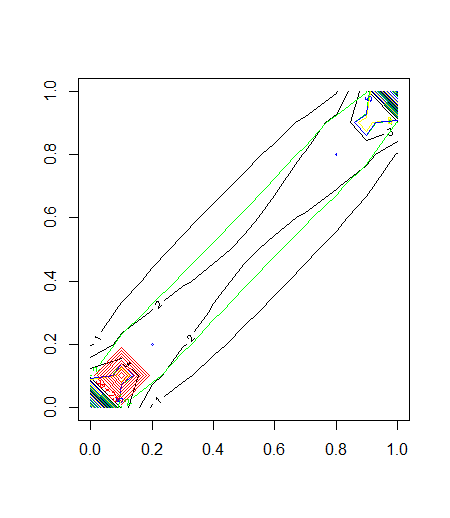
(a) Small effect size

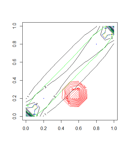
(b) Medium effect size

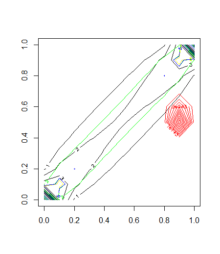
(c) Large effect size

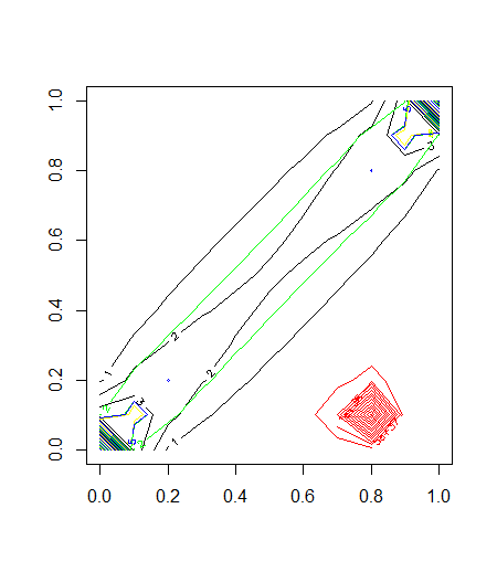
(d) XLarge effect size

Figure 2: $2\times 2$ table under product binomial ($n_{1}=n_{2}=n=100$) with values of effect size ”S”, ”M”, ”L”, ”XL”. Contour plots of intrinsic priors: $q=0.25$ (black), $q=0.5$ (green), $q=0.75$ (yellow), and (normalized) likelihood (red).

Tables 3 and 4 report the median (across the 200 simulations) of the posterior probabilities of the null model, $\mathrm{Pr}^{I}(M_{0}|t,\bm{y})$, and of the correct model, $\mathrm{Pr}^{I}(M_{c}|t,\bm{y})$, for selected values of the fraction $q$ of the training sample size. Both for contingency tables $2\times 2$ and $3\times 2$ two sets of model comparison were considered: $\{M_{0},M_{c},M_{e}\}$ and $\{M_{0},M_{c}\}$. Within each set the prior on models is taken to be uniform.

Consider first Table 3. If the model set is $\{M_{0},M_{c},M_{e}\}$ , the posterior probability of the true model $M_{c}$ is in the range 50%-99% across all scenarios, with values increasing as the effect size becomes larger. In particular, posterior probabilities between 50% and 60% occur only when the ES is either Small or Medium, whereas they are never below the threshold 77% when the ES is Large or XLarge. If however the comparison is restricted to the pair $\{M_{0},M_{c}\}$ the above range drastically shrinks to 83%-99% with a similar behavior with respect to increasing levels of ES. There is also a remarkable robustness to varying levels of $q$. Broadly similar considerations apply to Table 4; we omit details in the interest of brevity. In conclusion our method is able to identify the true model even when the effect size is small (e.g. using a conventional threshold of 50%), exhibits very limited sensitivity to the size of the imaginary sample used to construct the intrinsic prior, and behaves sensibly with regard to increasing levels of effect size.

Table 3: Simulation study for $2\times 2$ contingency tables. Median of the posterior model probabilities as a function of $q$ for distinct model comparison sets. Notice that in the labels of the columns the notation of the posterior model probability is $\mathrm{Pr}^{I}_{t,\bm{y}}(M)$ instead of $\mathrm{Pr}^{I}(M|t,\bm{y})$.

	# S1			# S2			# S3
	$M_{0}$-$M_{c}$-$M_{e}$		$M_{0}$-$M_{c}$	$M_{0}$-$M_{c}$-$M_{e}$		$M_{0}$-$M_{c}$	$M_{0}$-$M_{c}$-$M_{e}$		$M_{0}$-$M_{c}$
$q$	$\mathrm{Pr}^{I}_{t,\bm{y}}(M_{0})$	$\mathrm{Pr}^{I}_{t,\bm{y}}(M_{c})$	$\mathrm{Pr}^{I}_{t,\bm{y}}(M_{c})$	$\mathrm{Pr}^{I}_{t,\bm{y}}(M_{0})$	$\mathrm{Pr}^{I}_{t,\bm{y}}(M_{c})$	$\mathrm{Pr}^{I}_{t,\bm{y}}(M_{c})$	$\mathrm{Pr}^{I}_{t,\bm{y}}(M_{0})$	$\mathrm{Pr}^{I}_{t,\bm{y}}(M_{c})$	$\mathrm{Pr}^{I}_{t,\bm{y}}(M_{c})$
0	0.035	0.593	0.862	0.040	0.565	0.892	0.037	0.587	0.892
0.25	0.036	0.682	0.847	0.035	0.593	0.894	0.036	0.597	0.892
0.5	0.038	0.581	0.832	0.035	0.609	0.894	0.039	0.521	0.891
0.75	0.055	0.571	0.900	0.052	0.601	0.892	0.038	0.548	0.891
1	0.067	0.504	0.873	0.041	0.616	0.894	0.039	0.567	0.890
	# M1			# M2			# M3
	$M_{0}$-$M_{c}$-$M_{e}$		$M_{0}$-$M_{c}$	$M_{0}$-$M_{c}$-$M_{e}$		$M_{0}$-$M_{c}$	$M_{0}$-$M_{c}$-$M_{e}$		$M_{0}$-$M_{c}$
$q$	$\mathrm{Pr}^{I}_{t,\bm{y}}(M_{0})$	$\mathrm{Pr}^{I}_{t,\bm{y}}(M_{c})$	$\mathrm{Pr}^{I}_{t,\bm{y}}(M_{c})$	$\mathrm{Pr}^{I}_{t,\bm{y}}(M_{0})$	$\mathrm{Pr}^{I}_{t,\bm{y}}(M_{c})$	$\mathrm{Pr}^{I}_{t,\bm{y}}(M_{c})$	$\mathrm{Pr}^{I}_{t,\bm{y}}(M_{0})$	$\mathrm{Pr}^{I}_{t,\bm{y}}(M_{c})$	$\mathrm{Pr}^{I}_{t,\bm{y}}(M_{c})$
0	0.026	0.571	0.842	0.028	0.591	0.863	0.030	0.600	0.887
0.25	0.027	0.608	0.857	0.026	0.587	0.864	0.028	0.582	0.896
0.5	0.028	0.626	0.859	0.029	0.607	0.865	0.025	0.606	0.896
0.75	0.022	0.594	0.860	0.026	0.617	0.866	0.026	0.600	0.894
1	0.022	0.541	0.821	0.028	0.610	0.865	0.029	0.605	0.895
	# L1			# L2			# L3
	$M_{0}$-$M_{c}$-$M_{e}$		$M_{0}$-$M_{c}$	$M_{0}$-$M_{c}$-$M_{e}$		$M_{0}$-$M_{c}$	$M_{0}$-$M_{c}$-$M_{e}$		$M_{0}$-$M_{c}$
$q$	$\mathrm{Pr}^{I}_{t,\bm{y}}(M_{0})$	$\mathrm{Pr}^{I}_{t,\bm{y}}(M_{c})$	$\mathrm{Pr}^{I}_{t,\bm{y}}(M_{c})$	$\mathrm{Pr}^{I}_{t,\bm{y}}(M_{0})$	$\mathrm{Pr}^{I}_{t,\bm{y}}(M_{c})$	$\mathrm{Pr}^{I}_{t,\bm{y}}(M_{c})$	$\mathrm{Pr}^{I}_{t,\bm{y}}(M_{0})$	$\mathrm{Pr}^{I}_{t,\bm{y}}(M_{c})$	$\mathrm{Pr}^{I}_{t,\bm{y}}(M_{c})$
0	0.049	0.690	0.934	0.045	0.682	0.922	0.048	0.682	0.954
0.25	0.040	0.682	0.935	0.042	0.728	0.928	0.042	0.656	0.952
0.5	0.041	0.699	0.936	0.042	0.708	0.955	0.043	0.720	0.951
0.75	0.043	0.691	0.950	0.044	0.715	0.955	0.044	0.716	0.949
1	0.040	0.699	0.938	0.041	0.715	0.940	0.045	0.716	0.949
	# XL1			# XL2			# XL3
	$M_{0}$-$M_{c}$-$M_{e}$		$M_{0}$-$M_{c}$	$M_{0}$-$M_{c}$-$M_{e}$		$M_{0}$-$M_{c}$	$M_{0}$-$M_{c}$-$M_{e}$		$M_{0}$-$M_{c}$
$q$	$\mathrm{Pr}^{I}_{t,\bm{y}}(M_{0})$	$\mathrm{Pr}^{I}_{t,\bm{y}}(M_{c})$	$\mathrm{Pr}^{I}_{t,\bm{y}}(M_{c})$	$\mathrm{Pr}^{I}_{t,\bm{y}}(M_{0})$	$\mathrm{Pr}^{I}_{t,\bm{y}}(M_{c})$	$\mathrm{Pr}^{I}_{t,\bm{y}}(M_{c})$	$\mathrm{Pr}^{I}_{t,\bm{y}}(M_{0})$	$\mathrm{Pr}^{I}_{t,\bm{y}}(M_{c})$	$\mathrm{Pr}^{I}_{t,\bm{y}}(M_{c})$
0	0.059	0.862	0.995	0.074	0.867	0.995	0.069	0.895	0.997
0.25	0.061	0.856	0.992	0.070	0.862	0.986	0.065	0.898	0.991
0.5	0.056	0.858	0.991	0.071	0.862	0.981	0.070	0.900	0.990
0.75	0.072	0.858	0.989	0.069	0.863	0.975	0.070	0.900	0.993
1	0.075	0.858	0.989	0.071	0.863	0.970	0.073	0.899	0.999

Table 4: Simulation study for $3\times 2$ contingency tables. Median of the posterior model probabilities as a function of $q$ for distinct model comparison sets. Notice that in the labels of the columns the notation of the posterior model probability is $\mathrm{Pr}^{I}_{t,\bm{y}}(M)$ instead of $\mathrm{Pr}^{I}(M|t,\bm{y})$.

	# S1			# S2			# S3
	$M_{0}$-$M_{c}$-$M_{e}$		$M_{0}$-$M_{c}$	$M_{0}$-$M_{c}$-$M_{e}$		$M_{0}$-$M_{c}$	$M_{0}$-$M_{c}$-$M_{e}$		$M_{0}$-$M_{c}$
$q$	$\mathrm{Pr}^{I}_{t,\bm{y}}(M_{0})$	$\mathrm{Pr}^{I}_{t,\bm{y}}(M_{c})$	$\mathrm{Pr}^{I}_{t,\bm{y}}(M_{c})$	$\mathrm{Pr}^{I}_{t,\bm{y}}(M_{0})$	$\mathrm{Pr}^{I}_{t,\bm{y}}(M_{c})$	$\mathrm{Pr}^{I}_{t,\bm{y}}(M_{c})$	$\mathrm{Pr}^{I}_{t,\bm{y}}(M_{0})$	$\mathrm{Pr}^{I}_{t,\bm{y}}(M_{c})$	$\mathrm{Pr}^{I}_{t,\bm{y}}(M_{c})$
0	0.025	0.565	0.611	0.021	0.569	0.655	0.022	0.557	0.656
0.25	0.023	0.565	0.596	0.021	0.569	0.616	0.024	0.565	0.646
0.5	0.018	0.570	0.613	0.022	0.577	0.682	0.024	0.568	0.666
0.75	0.021	0.572	0.630	0.022	0.582	0.660	0.024	0.580	0.669
1	0.031	0.574	0.654	0.030	0.587	0.679	0.025	0.575	0.674
	# M1			# M2			# M3
	$M_{0}$-$M_{c}$-$M_{e}$		$M_{0}$-$M_{c}$	$M_{0}$-$M_{c}$-$M_{e}$		$M_{0}$-$M_{c}$	$M_{0}$-$M_{c}$-$M_{e}$		$M_{0}$-$M_{c}$
$q$	$\mathrm{Pr}^{I}_{t,\bm{y}}(M_{0})$	$\mathrm{Pr}^{I}_{t,\bm{y}}(M_{c})$	$\mathrm{Pr}^{I}_{t,\bm{y}}(M_{c})$	$\mathrm{Pr}^{I}_{t,\bm{y}}(M_{0})$	$\mathrm{Pr}^{I}_{t,\bm{y}}(M_{c})$	$\mathrm{Pr}^{I}_{t,\bm{y}}(M_{c})$	$\mathrm{Pr}^{I}_{t,\bm{y}}(M_{0})$	$\mathrm{Pr}^{I}_{t,\bm{y}}(M_{c})$	$\mathrm{Pr}^{I}_{t,\bm{y}}(M_{c})$
0	0.021	0.576	0.693	0.029	0.588	0.769	0.025	0.558	0.703
0.25	0.021	0.573	0.712	0.029	0.587	0.817	0.025	0.558	0.759
0.5	0.023	0.576	0.770	0.029	0.588	0.798	0.025	0.556	0.779
0.75	0.022	0.579	0.743	0.029	0.588	0.794	0.026	0.559	0.789
1	0.022	0.580	0.763	0.028	0.588	0.796	0.025	0.560	0.783
	# L1			# L2			# L3
	$M_{0}$-$M_{c}$-$M_{e}$		$M_{0}$-$M_{c}$	$M_{0}$-$M_{c}$-$M_{e}$		$M_{0}$-$M_{c}$	$M_{0}$-$M_{c}$-$M_{e}$		$M_{0}$-$M_{c}$
$q$	$\mathrm{Pr}^{I}_{t,\bm{y}}(M_{0})$	$\mathrm{Pr}^{I}_{t,\bm{y}}(M_{c})$	$\mathrm{Pr}^{I}_{t,\bm{y}}(M_{c})$	$\mathrm{Pr}^{I}_{t,\bm{y}}(M_{0})$	$\mathrm{Pr}^{I}_{t,\bm{y}}(M_{c})$	$\mathrm{Pr}^{I}_{t,\bm{y}}(M_{c})$	$\mathrm{Pr}^{I}_{t,\bm{y}}(M_{0})$	$\mathrm{Pr}^{I}_{t,\bm{y}}(M_{c})$	$\mathrm{Pr}^{I}_{t,\bm{y}}(M_{c})$
0	0.033	0.770	0.980	0.032	0.777	0.976	0.029	0.818	0.973
0.25	0.031	0.768	0.973	0.035	0.788	0.978	0.030	0.818	0.972
0.5	0.033	0.810	0.979	0.035	0.781	0.974	0.030	0.812	0.972
0.75	0.033	0.808	0.979	0.035	0.789	0.974	0.031	0.816	0.972
1	0.033	0.801	0.979	0.036	0.788	0.973	0.030	0.811	0.972
	# XL1			# XL2			# XL3
	$M_{0}$-$M_{c}$-$M_{e}$		$M_{0}$-$M_{c}$	$M_{0}$-$M_{c}$-$M_{e}$		$M_{0}$-$M_{c}$	$M_{0}$-$M_{c}$-$M_{e}$		$M_{0}$-$M_{c}$
$q$	$\mathrm{Pr}^{I}_{t,\bm{y}}(M_{0})$	$\mathrm{Pr}^{I}_{t,\bm{y}}(M_{c})$	$\mathrm{Pr}^{I}_{t,\bm{y}}(M_{c})$	$\mathrm{Pr}^{I}_{t,\bm{y}}(M_{0})$	$\mathrm{Pr}^{I}_{t,\bm{y}}(M_{c})$	$\mathrm{Pr}^{I}_{t,\bm{y}}(M_{c})$	$\mathrm{Pr}^{I}_{t,\bm{y}}(M_{0})$	$\mathrm{Pr}^{I}_{t,\bm{y}}(M_{c})$	$\mathrm{Pr}^{I}_{t,\bm{y}}(M_{c})$
0	0.075	0.862	0.993	0.045	0.873	0.997	0.065	0.883	0.998
0.25	0.081	0.857	0.998	0.045	0.877	0.999	0.069	0.890	0.999
0.5	0.052	0.864	0.997	0.045	0.876	0.999	0.068	0.889	0.998
0.75	0.057	0.867	0.997	0.046	0.876	0.999	0.068	0.889	0.999
1	0.065	0.868	0.997	0.045	0.878	0.999	0.067	0.889	0.999

5.2 Real data analyses

In this subsection we apply our method to real datasets and compare our results with previously analyzed studies. One aspect which we further consider is the robustness of our conclusions to the choice of the hyper-parameter $q$ which represents the fraction of the training sample size, relative to the actual sample size, which is used to construct the intrinsic prior. Assuming lack of prior information, all models under consideration are given a priori the same probability. Different prior model probabilities can be easily accommodated within our framework.

5.2.1 Product binomial model

Trauma due to subarachnoid hemorrhage.

We return to Table 1 of Section 3 which reports the response to different treatments of patients who experienced trauma due to subarachnoid hemorrhage (Agresti & Coull, 2002). This is a $4\times 2$ contingency table whose columns are the response categories (“dead” or “not dead ”) while the rows contain three ordered levels of medication dose plus a control group. The objective of the study is to determine whether a more favorable outcome tends to occur as the dose increases. Using the notation of Section 3 there are three possible models that we can consider, namely

$$M_{0}:\, \pi_{1}=\pi_{2}=\pi_{3}=\pi_{4}$$

$$M_{c}:\, \pi_{1}>\pi_{2}>\pi_{3}>\pi_{4}$$

$$M_{e}:\, (\pi_{i},i=1,\dots,4)\in\{[0,1]^{4}\setminus\{\pi_{1}=\ldots=\pi_{4}\}\}.$$

Agresti & Coull (2002) analyzed these data using a frequentist approach. Specifically, they tested the null model of equal probabilities $M_{0}$ against that of ordered alternatives $M_{c}$ using the large-sample chi-bar squared distribution, and obtained a $p$-value equal to 0.095, so that the null model cannot be rejected using default settings. However they correctly point out that this result does not enable one to conclude how strong is the evidence in favor of the null. The latter instead is available using our approach.

Table 5: Trauma due to subarachnoid hemorrhage. Bayes factors as a function of $q$.

$q$	$BF^{I}_{e0}$	$BF^{I}_{ce}$	$BF^{I}_{c0}$
0	12.965	1.017	13.189
0.25	144.197	2.172	313.259
0.5	147.798	2.752	406.793
0.75	123.942	3.336	413.453
1	93.672	3.737	350.017

Table 6: Trauma due to subarachnoid hemorrhage. Posterior model probabilities as a function of $q$ for distinct model comparison sets.

	$M_{0}$ - $M_{e}$		$M_{0}$ - $M_{c}$		$M_{0}$ - $M_{c}$ - $M_{e}$
$q$	$\mathrm{Pr}^{I}(M_{0}|t,\bm{y})$	$\mathrm{Pr}^{I}(M_{e}|t,\bm{y})$	$\mathrm{Pr}^{I}(M_{0}|t,\bm{y})$	$\mathrm{Pr}^{I}(M_{c}|t,\bm{y})$	$\mathrm{Pr}^{I}(M_{0}|t,\bm{y})$	$\mathrm{Pr}^{I}(M_{c}|t,\bm{y})$	$\mathrm{Pr}^{I}(M_{e}|t,\bm{y})$
0	0.072	0.923	0.070	0.930	0.037	0.504	0.459
0.25	0.007	0.993	0.003	0.997	0.002	0.685	0.313
0.5	0.007	0.993	0.002	0.998	0.002	0.733	0.265
0.75	0.008	0.992	0.002	0.998	0.002	0.769	0.229
1	0.011	0.990	0.003	0.997	0.002	0.789	0.209

Table 5 reports, for selected values of $q$, the Bayes factors $BF^{I}_{e0}$, $BF^{I}_{ce}$ and $BF^{I}_{c0}$ (the last one being of course a function of the former two). It appears that both the unconstrained and the constrained model are strongly supported by the data relative to the null model of independence with values of $BF^{I}_{e0}$ over 100 and those of $BF^{I}_{c0}$ over 300 for $q\geq 0.25$. In other words the strength of evidence (Schönbrodt & Wagenmakers, 2018) against the null is extreme whether the comparison is made against the unconstrained or the constrained model. Additionally the Bayes factor for comparing $M_{c}$ against $M_{e}$ suggests values greater than 1 and extending beyond 3.5. Although this represents only anecdotal, or at most moderate evidence, in favor of $M_{c}$, it nevertheless indicates that $M_{c}$ is somewhat better supported by the data than $M_{e}$. Table 6 allows a finer appreciation of the main features of our analysis, as it reports the posterior probability of each model separately for each of the three sets of model comparison, namely $\{M_{0},M_{e}\}$, $\{M_{0},M_{c}\}$ and $\{M_{0},M_{c},M_{e}\}$. It appears that the evidence in favor of the null, $Pr^{I}(M_{0}|t,\bf{y})$, is very small, its value never exceeding $7\%$ while being most of the time a tenth of the above or lower. Accordingly the constrained model $M_{c}$ receives a very high posterior probability (above 90%) when the comparison is restricted to $\{M_{0},M_{c}\}$; this value somewhat diminishes (being around 70%) when also the unconstrained model is taken into consideration. We therefore conclude that evidence in favor of the constrained model $M_{c}$ is strong and that this result is robust to variations in $q$.

We highlight the fact that the constrained model $M_{c}$ and the unconstrained model $M_{e}$ have the same dimension. Nevertheless $M_{c}$ is nested into, and so less complex than, $M_{e}$ because of its smaller parameter space. Interestingly, $M_{c}$ receives a much higher posterior probability than $M_{e}$ as it is apparent from scenario $\{M_{0},M_{c},M_{e}\}$, at least for $q\geq 0.25$. This occurs because of the more complex models are penalized due to Ockham’s razor (Jefferys & Berger, 1992). We therefore conclude that not only is the null model of independence to be discarded, but there is clear evidence in favor of the constrained model.

5.2.2 Multinomial model

Surgical methods for ulcer treatment.

Efron (1996) analyzed data coming from a multicenter trial whose objective was to establish whether a new surgical method (Treatment) for ulcer was superior to an older one (Control) with regard to reducing recurrent bleeding. The data refer to 41 hospitals. For each hospital a $2\times 2$ contingency table summarizes the results. Each table is presented as $(a,b;c,d)$, where $(a,b)$ are the number of occurrences and non-occurrences for the Treatment, while $(c,d)$ are the corresponding values for the Control; here occurrence refers to recurrent bleeding.

Casella & Moreno (2009) tested in each contingency table independence between occurrence and method of surgery (model $M_{0}$) against an unconstrained alternative ($M_{e}$):

$$M_{0} : \pi_{ij}=\theta_{i}\cdot\eta_{j};\,\forall i,j\in\{1,2\}\,(0<\theta_{1}<1;0<\eta_{1}<1;\,\theta_{1}+\theta_{2}=1;\,\eta_{1}+\eta_{2}=1)$$

$$M_{e} : 0<\pi_{ij}<1;\,(\pi_{11}+\pi_{12}+\pi_{21}+\pi_{22}=1).$$ (27)

Letting $\theta_{1}=\theta$ and $\eta_{1}=\eta$, they used the following default priors

$$p^{N}(\theta,\eta|M_{0}) = p^{N}(\theta|M_{0})p^{N}(\eta|M_{0})=Unif(\theta;0,1)Unif(\eta;0,1)$$

$$p^{N}(\bm{\pi}|M_{e}) = Di(\bm{\pi}|1,1,1,1).$$ (28)

Next they constructed an intrinsic prior under $M_{e}$ letting the training sample size $t$ range over the set $0,\ldots,n$. Their results are reported in Table 7 for five selected hospitals arranged according to increasing $p$-values. Although the posterior probability of the null model is conceptually quite different from the $p$-value (Wasserstein & Lazar, 2016), one can see that it generally increases with the $p$-value correctly reporting higher evidence in favor of the null. However only for one hospital (# 18) does the posterior probability of the null exceeds the 0.5 threshold (when $q=0)$, and even in this case the result is not robust because it goes below this value when $q=1$. Based on the intrinsic analysis they conclude that for none of these hospitals there exists a robust support for the null hypothesis of independence of surgery and occurrence.

Table 7: Selected contingency tables from Efron (1996). Posterior probability of the null model based on the intrinsic prior approach for $t=0$ and $t=n$. (The notation (a,b;c,d) denotes a $2\times 2$ table with first row (a,b) reporting adverse occurences and non occurrences for the new surgery and similarly for the second row (c,d) which refers to the old surgery. $n=a+b+c+d$). Table adapted from Casella & Moreno (2009, Table 2)

Hospital number	Data	$p$-value	$\mathrm{Pr}^{I}(M_{0}|t,\bm{y})$
			$t=0$	$t=n$
34	(20,0;18,5)	0.051	0.215	0.215
1	(8,7;2,11)	0.054	0.170	0.253
38	(43,4;14,5)	0.106	0.395	0.340
18	(30,1;23,4)	0.173	0.551	0.406
16	(7,4;4,6)	0.395	0.451	0.497

A natural hypothesis underlying Efron’s data is that the new surgery is superior to the old one, i.e. the probability of occurrence within Treatment is lower than the corresponding probability under Control. However this feature is not taken into account in the previous analysis. Accordingly, we reanalyze Efron’s tables explicitly accounting for this hypothesis which we can write as:

$$M_{c}:\frac{\pi_{11}}{\pi_{11}+\pi_{12}}<\frac{\pi_{21}}{\pi_{21}+\pi_{22}},$$

equivalently $Pr(\mbox{occurrence}|\mbox{Treament})<Pr(\mbox{occurrence}|\mbox{Control})$.

Tables 8 and 9 present our results which are obtained using default priors specified in (5.2.2).

Table 8: Selected contingency tables from Efron (1996). Bayes factors appearing in formula (13) as a function of $q$.

	Table 34			Table 1			Table 38
$q$	$BF^{I}_{e0}$	$BF^{I}_{ce}$	$BF^{I}_{c0}$	$BF^{I}_{e0}$	$BF^{I}_{ce}$	$BF^{I}_{c0}$	$BF^{I}_{e0}$	$BF^{I}_{ce}$	$BF^{I}_{c0}$
0	3.648	0.993	3.624	4.892	0.996	4.875	1.529	0.987	1.509
0.25	4.812	0.593	2.852	4.003	0.559	2.241	2.052	0.478	0.982
0.5	4.758	0.395	1.879	3.438	0.379	1.306	2.064	0.337	0.695
0.75	4.392	0.277	1.218	3.148	0.278	0.875	2.002	0.255	0.511
1	4.054	0.201	0.816	2.882	0.208	0.601	1.913	0.192	0.368
	Table 18			Table 16
$q$	$BF^{I}_{e0}$	$BF^{I}_{ce}$	$BF^{I}_{c0}$	$BF^{I}_{e0}$	$BF^{I}_{ce}$	$BF^{I}_{c0}$
0	0.815	1.007	0.821	1.217	0.998	1.216
0.25	1.305	0.683	0.891	1.071	0.765	0.819
0.5	1.439	0.506	0.727	0.996	0.676	0.674
0.75	1.46	0.425	0.620	0.986	0.588	0.579
1	1.439	0.351	0.505	1.000	0.525	0.525

Table 9: Selected contingency tables from Efron (1996). Posterior model probabilities, as a function of $q$ for different comparison scenarios

Table		$M_{0}$ - $M_{e}$		$M_{0}$ - $M_{c}$		$M_{0}$ - $M_{c}$ - $M_{e}$
34	$q$	$\mathrm{Pr}^{I}(M_{0}|t,\bm{y})$	$\mathrm{Pr}^{I}(M_{e}|t,\bm{y})$	$\mathrm{Pr}^{I}(M_{0}|t,\bm{y})$	$\mathrm{Pr}^{I}(M_{c}|t,\bm{y})$	$\mathrm{Pr}^{I}(M_{0}|t,\bm{y})$	$\mathrm{Pr}^{I}(M_{c}|t,\bm{y})$	$\mathrm{Pr}^{I}(M_{e}|t,\bm{y})$
	0	0.215	0.785	0.216	0.7837	0.121	0.438	0.441
	0.25	0.172	0.828	0.234	0.766	0.115	0.329	0.555
	0.5	0.174	0.826	0.302	0.698	0.131	0.246	0.623
	0.75	0.185	0.815	0.379	0.620	0.151	0.184	0.664
	1	0.198	0.802	0.470	0.529	0.170	0.139	0.691
1	$q$	$\mathrm{Pr}^{I}(M_{0}|t,\bm{y})$	$\mathrm{Pr}^{I}(M_{e}|t,\bm{y})$	$\mathrm{Pr}^{I}(M_{0}|t,\bm{y})$	$\mathrm{Pr}^{I}(M_{c}|t,\bm{y})$	$\mathrm{Pr}^{I}(M_{0}|t,\bm{y})$	$\mathrm{Pr}^{I}(M_{c}|t,\bm{y})$	$\mathrm{Pr}^{I}(M_{e}|t,\bm{y})$
	0	0.170	0.830	0.170	0.829	0.0929	0.4528	0.454
	0.25	0.200	0.800	0.313	0.687	0.138	0.309	0.553
	0.5	0.225	0.775	0.454	0.546	0.174	0.227	0.598
	0.75	0.258	0.742	0.574	0.426	0.199	0.174	0.627
	1	0.258	0.742	0.258	0.742	0.223	0.134	0.643
38	$q$	$\mathrm{Pr}^{I}(M_{0}|t,\bm{y})$	$\mathrm{Pr}^{I}(M_{e}|t,\bm{y})$	$\mathrm{Pr}^{I}(M_{0}|t,\bm{y})$	$\mathrm{Pr}^{I}(M_{c}|t,\bm{y})$	$\mathrm{Pr}^{I}(M_{0}|t,\bm{y})$	$\mathrm{Pr}^{I}(M_{c}|t,\bm{y})$	$\mathrm{Pr}^{I}(M_{e}|t,\bm{y})$
	0	0.395	0.605	0.398	0.601	0.248	0.374	0.379
	0.25	0.328	0.672	0.481	0.519	0.248	0.243	0.509
	0.5	0.326	0.674	0.554	0.446	0.266	0.185	0.549
	0.75	0.333	0.667	0.617	0.382	0.285	0.145	0.569
	1	0.343	0.657	0.683	0.317	0.305	0.112	0.583
18	$q$	$\mathrm{Pr}^{I}(M_{0}|t,\bm{y})$	$\mathrm{Pr}^{I}(M_{e}|t,\bm{y})$	$\mathrm{Pr}^{I}(M_{0}|t,\bm{y})$	$\mathrm{Pr}^{I}(M_{c}|t,\bm{y})$	$\mathrm{Pr}^{I}(M_{0}|t,\bm{y})$	$\mathrm{Pr}^{I}(M_{c}|t,\bm{y})$	$\mathrm{Pr}^{I}(M_{e}|t,\bm{y})$
	0	0.551	0.449	0.549	0.451	0.379	0.311	0.309
	0.25	0.434	0.566	0.495	0.505	0.313	0.279	0.408
	0.5	0.410	0.590	0.518	0.482	0.316	0.230	0.454
	0.75	0.406	0.594	0.539	0.461	0.325	0.2014	0.474
	1	0.410	0.590	0.408	0.592	0.340	0.172	0.489
16	$q$	$\mathrm{Pr}^{I}(M_{0}|t,\bm{y})$	$\mathrm{Pr}^{I}(M_{e}|t,\bm{y})$	$\mathrm{Pr}^{I}(M_{0}|t,\bm{y})$	$\mathrm{Pr}^{I}(M_{c}|t,\bm{y})$	$\mathrm{Pr}^{I}(M_{0}|t,\bm{y})$	$\mathrm{Pr}^{I}(M_{c}|t,\bm{y})$	$\mathrm{Pr}^{I}(M_{e}|t,\bm{y})$
	0	0.451	0.549	0.451	0.549	0.291	0.354	0.355
	0.25	0.483	0.517	0.553	0.447	0.346	0.284	0.370
	0.5	0.501	0.499	0.605	0.395	0.374	0.252	0.373
	0.75	0.504	0.496	0.650	0.349	0.389	0.226	0.384
	1	0.498	0.502	0.674	0.326	0.396	0.208	0.396

First notice that the values of $\mathrm{Pr}^{I}(M_{0}|t=0,\bm{y})$ in the $\{M_{0},M_{e}\}$ scenario coincide with those of in Table 2 of Casella & Moreno (2009) under their “Uniform” column because in that case the priors used in the calculation are the default priors (5.2.2). (As usual, we index our table with $q=t/n$, so that the case $t=0$ coincides with $q=0$. It can be checked that the results for $t=0$ also coincide with those of $t=1$ because of the structure of formula (26)).

The results of Table 9 can be summarized as follows:

• For hospitals 34 and 1 there is robust evidence against $M_{0}$ because its posterior probability is always well below the 50% threshold, whatever scenario is considered. When all three models are entertained, it appears that the unconstrained model $M_{e}$ is better supported than $M_{c}$, because its posterior probability exceeds 50% save for $q=0$ (the default starting case which is not recommended for model comparison).

• For hospitals 18 and 16 the situation is rather different. The null model of independence achieves values of posterior probability around 40% when compared against $M_{e}$; but this probability increases and exceeds 1/2 when the comparison is against $M_{c}$: this is especially true for hospital 16. When all three models are considered jointly it appears that the unconstrained model prevails although by a moderate amount; interestingly the next better supported model is that of independence, while the constrained model typically scores the least value.

• Finally, for hospital 38 the null model of independence is less supported than for hospitals 18 and 16. In the $\{M_{0},M_{e}\}$ scenario there is robust but moderate evidence for $M_{e}$ (the posterior probability being always greater than 0.6); however this is not the case in the scenario $\{M_{0},M_{c}\}$ where $M_{0}$ receives higher evidence than $M_{c}$ save for $q=0$ and $q=0.25$.

  This item is interesting because it reveals that, by focussing our testing procedure more narrowly on the constrained model (a more reasonable alternative in the context of medical treatment), the null hypothesis comes out as being more supported by the data.

Self-perception and behavior of students.

Nash & Bowen (2002) considered the relation between perception of internal strength and resources (“Internal Assets”) and class behavior among students in grades from 6 to 12. Data were collected using the School Success Profile, a self administered instrument designed for students. The Internal Assets Index is a measure of the adolescent’s perception of his or her strength and resources (health, exercises, or involvement in sports), which for this study was categorized into “low” and “high”. Each student was also asked whether he or she during the previous 30 days had been sent away from class because of his or her behavior. The data are displayed in Table 10 where one can verify that the frequency of being sent away from class in the “low” group is only moderately larger than in the “high” group ($0.172>0.136$).

Table 10: Contingency table $2\times 2$ taken from Table 3 of Klugkist et al. (2010)

Internal Assets	Sent Away from Class
	yes	no
low	220	1060
high	96	609

These data were analyzed by Klugkist et al. (2010) by testing a constrained model $M_{c}$ (students with low internal assets are more likely to be sent away from class than students with high internal assets) against the null model $M_{0}$ of no difference between the two groups; they also considered an unconstrained model $M_{e}$ as a possible explanation. (Labels for the hypotheses are consistent with the notation in this paper but different from theirs). Models $M_{0}$ and $M_{e}$ are defined as in (5.2.2), and default priors as in (5.2.2).

On the other hand model $M_{c}$ is now specified as

$$M_{c}:\frac{\pi_{11}}{\pi_{11}+\pi_{12}}>\frac{\pi_{21}}{\pi_{21}+\pi_{22}},$$

Klugkist et al. (2010) assign only one prior under $M_{e}$, namely $Dir(\bf{\pi}|1,1,1,1)$ and regard both $M_{0}$ and $M_{e}$ as constrained models; accordingly they induce priors under the two latter models using an encompassing approach. This however presents a technical difficulty because $M_{0}$ involves only equality constraints which cannot be dealt with directly because the null parameter space is a set of probability zero under the above prior. This leads them to define “about equality” constraints to accommodate the analysis of this problem into their framework. As a consequence they are forced to introduce thresholds in order to define “about equality”, thus adding an arbitrary step. On the other hand our method treats $M_{0}$ as a separate model with its own parameter and prior.

Their analysis leads to the following Bayes factors $BF_{ce}(\bm{y})=1.97$ and $BF_{0e}(\bm{y})=2.59$ which shows that the constrained model is better supported than the unconstrained model, however it is the null model which receives higher support. The corresponding model posterior probabilties are $\mathrm{Pr}(M_{0}|{\bf{y}})=0.47$, $\mathrm{Pr}(M_{c}|{\bf{y}})=0.35$, $\mathrm{Pr}(M_{e}|{\bf{y}})=0.18$, so that the null model of independence appears as the most likely followed by that which assumes a constraint and finally by the unconstrained model.

Table 11: Self-perception and behavior of students. Bayes factors appearing in formula (13) as a function of $q$.

$q$	$BF^{I}_{e0}$	$BF^{I}_{ce}$	$BF^{I}_{c0}$
0	0.4199	1.5386	0.6461
0.25	0.4237	1.5375	0.6515
0.5	0.3864	1.6957	0.6552
0.75	0.3870	1.7893	0.6925
1	0.4035	1.8531	0.7477

We report in Table 11 the Bayes factors generated by our approach. The values of $BF^{I}_{e0}$ suggest that evidence in favor of $M_{e}$ is less than half that of $M_{0}$; additionally evidence for $M_{c}$ is about one-and-half that for $M_{e}$; as a consequence the evidence for the constrained model $BF^{I}_{c0}=BF^{I}_{e0}\cdot BF^{I}_{ce}$ ranges between 0.65 and 0.75. We highlight the fact that there is a good degree of robustness wrt $q$.

In Table 12 we report the posterior model probabilities for three distinct comparison scenarios.

Table 12: Self-perception and behavior of students. Posterior model probabilities as a function of $q$ for different model comparison scenarios

	$M_{0}$ - $M_{e}$		$M_{0}$ - $M_{c}$		$M_{0}$ - $M_{c}$ - $M_{e}$
$q$	$\mathrm{Pr}^{I}(M_{0}|t,\bm{y})$	$\mathrm{Pr}^{I}(M_{e}|t,\bm{y})$	$\mathrm{Pr}^{I}(M_{0}|t,\bm{y})$	$\mathrm{Pr}^{I}(M_{c}|t,\bm{y})$	$\mathrm{Pr}^{I}(M_{0}|t,\bm{y})$	$\mathrm{Pr}^{I}(M_{c}|t,\bm{y})$	$\mathrm{Pr}^{I}(M_{e}|t,\bm{y})$
0	0.7043	0.2957	0.6075	0.3925	0.4840	0.3127	0.2032
0.25	0.7024	0.2976	0.6055	0.3945	0.4819	0.3139	0.2042
0.5	0.7213	0.2787	0.6042	0.3958	0.4898	0.3209	0.1893
0.75	0.7210	0.2790	0.5904	0.4096	0.4808	0.3330	0.1861
1	0.7125	0.2875	0.5722	0.4278	0.4649	0.3476	0.1876

It appears from Table 12 that the null model of independence should be regarded as the one having the strongest evidential support, whatever the scenario under consideration. We believe that the most reasonable comparison setting for testing independence in this problem is the one involving $\{M_{0},M_{c}\}$ because the natural expectation is that students with low internal assets are more likely, if at all, to be sent away from class than students with high internal assets. This is also somewhat supported on purely descriptive grounds, as already recalled. In the above scenario, the posterior probability of $M_{0}$ ranges between 57 and 61% as $q$ varies; in other words there is evidence in favor of $H_{0}$ because the conventional $50\%$ threshold is exceeded, although its strength is not overwhelming. Interestingly when $M_{0}$ is contrasted with the unconstrained model $M_{e}$ its evidence increases to a comfortable 70%, and again this result is robust. The reason is clear: the alternative confronting $M_{0}$ is now less precise (the parameter space is larger) and, more importantly, in greater conflict with the likelihood than $M_{c}$ (recall that the frequency of being Sent Away from Class with low Internal assets is 0.172 whereas the corresponding frequency with high Internal Assets is 0.136, a lower value). As a consequence, its marginal likelihood is penalized and this is reflected in a lower (higher) posterior probability for $M_{e}$ ($M_{0})$. Finally, for the scenario involving three models $\{M_{0},M_{c},M_{e}\}$, $M_{0}$ remains the highest-posterior-probability model although its value drops to around 47-48%. This is only to be expected because we are now contrasting $M_{0}$ with two, rather than just one, competitors. We could view this comparative scenario as a sort of “stress test” for $M_{0}$, rather than a substantive research hypothesis. Since the threshold $50\%$ is only closely missed, evidence for $H_{0}$ seems worth of consideration.

6 Concluding remarks

In this paper we have presented an objective Bayes model comparison procedure for two-way contingency tables where models are specified by inequality constraints on the parameter space. Specifically we have considered contingency tables whose sampling distribution is either product multinomial (including product Binomial as a special case), or fully multinomial.

Our method relies on the principled method of intrinsic priors for model comparison coupled with the encompassing prior approach to compute the Bayes factor and the posterior probability of each constrained model.

An attractive feature of our method is that it requires no subjective input, but merely standard default priors, which makes it essentially fully automatic. When the default prior, as in our examples, is already proper, we can assess the robustness of our inference by letting the fraction of prior sample size to actual sample size vary: if the result is always above a threshold deemed to represent sufficient evidence, then we can safely conclude that the result is robust. Our method can also deal with starting default improper priors however, such as the Jeffreys prior $\mbox{Beta}(1/2,1/2)$: in this case however we would recommend using conditionally intrinsic priors, as opposed to fully intrinsic priors: for details see Consonni & Paroli (2017).

Another interesting characteristic of our method is that it can deal simultaneously with nested models having different or equal dimensions of the parameter space. For instance, the constrained models in the examples of Section 5 were all of the same dimension as the unconstrained model. Since the Bayes factor has a built-in Ockam’s razor, it can well happen that the constrained model receives higher evidence than the encompassing model because it trades automatically fit and model complexity.

Using the general principles expounded in Consonni & Paroli (2017), the scope of our method can be extended to the comparison of models specified by equality and inequality constraints. This can be done exactly without resorting to approximate representations of equality constraints.

Appendix

Bayes Factor in the multinomial case

A1. Algorithm to estimate $BF^{I}_{e0}(\bm{y}|t)$

To estimate ${BF}^{I}_{e0}(\bm{y}|t)$ we use an importance sampling algorithm to compute the MonteCarlo sum.

Algorithm 3 Approximation of the ${BF}^{I}_{e0}(\bm{y}|t)$

1:for $s=1,2,\ldots,S$ do

2:     sample a contingency table $\bm{x}^{(s)}$ from the candidate distribution that is Multinomial with cell probabilities equal to the observed cell relative frequencies and with total sum equal to $t$:

$$\bm{x}^{(s)}\sim Multinomial(t,\bm{\hat{\pi}})$$

with $\bm{\hat{\pi}}=\{\hat{\pi}_{ij}=y_{ij}/n;i=1,\ldots,r;j=1,\ldots,c\}$;

3:     compute the product

$$q^{(s)}=\frac{(\prod_{i}x_{i+}^{(s)}!)(\prod_{j}x_{+j}^{(s)}!)}{\prod_{i}y_{i+}!)(\prod_{j}y_{+j}!)}\times\frac{\prod_{i,j}(x_{ij}^{(s)}+y_{ij})!}{\prod_{i,j}x_{ij}^{(s)}!}\times\frac{1}{\prod_{ij}\hat{\pi}_{ij}^{x_{ij}^{(s)}}}$$

where the last element is the importance density of the sampled table;

4:end for

5:approximate ${BF}^{I}_{e0}(\bm{y}|t)$ as

$$\widehat{BF}^{I}_{e0}(\bm{y}|t)\simeq\frac{\Gamma(t+rc)\Gamma(n+r)\Gamma(n+c)}{\Gamma(t+n+rc)\Gamma(t+r)\Gamma(t+c)}\times\frac{1}{S}\sum_{s=1}^{S}q^{(s)}.$$

A2. Algorithms to estimate $BF^{I}_{ce}(\bm{y}|t)$

To compute ${BF}^{I}_{ce}(\bm{y}|t)$ we use the same strategy discussed in par. (3.2)

• Consider first the evaluation of the denominator. We approximate the required probability by drawing $S$ samples from the intrinsic prior (17), check the constraints and compute the fraction of samples that satisfy them.

  Algorithm 4 Approximation of the denominator of ${BF}^{I}_{ce}(\bm{y}|t)$

  1:for $s=1,2,\ldots,S$ do

  2:     sample $\bm{\pi}^{*(s)}$ under the null model; i.e. sample the marginals $\bm{\pi_{1}}^{(s)}$ and $\bm{\pi_{2}}^{(s)}$ from their priors $\bm{\pi_{1}}^{(s)}\sim Dir(\bm{\alpha}_{\pi_{1}})$ and $\bm{\pi_{2}}^{(s)}\sim Dir(\bm{\alpha}_{\pi_{2}})$, and compute $\bm{\pi}^{*(s)}=\{\pi_{ij}^{*(s)}=\pi_{1i}^{(s)}\cdot\pi_{2j}^{(s)};i=1.\ldots,r;j=1,\ldots,c\}$;

  3:     sample a contingency table $\bm{x}^{(s)}$ from a Multinomial:

  $$\bm{x}^{(s)}\sim Multinomial(t,\bm{\pi}^{*(s)});$$

  4:     sample $\bm{\pi}^{(s)}$ from the pseudo posterior

  $$\bm{\pi}^{(s)}\sim Dir(\bm{\alpha}_{\pi}+\bm{x}^{(s)});$$

  5:end for

  6:approximate the probability in the denominator as

  $$\widehat{\mathrm{Pr}}^{I}\{\bm{\pi}\in\Theta_{c}|M_{e}\}\thickapprox\frac{1}{S}\sum_{s=1}^{S}\bm{1}_{\bm{\pi}\in\Theta_{c}}(\bm{\pi}^{(s)}).$$

• For the numerator of $BF^{I}_{ce}$ we rely on a Metropolis within Gibbs algorithm as follows:

  Algorithm 5 Approximation of the numerator of ${BF}^{I}_{ce}(\bm{y}|t)$

  1:estimate the probabilities $\bm{\pi}$ with the modified MLE estimators

  $$\widehat{\pi}_{ij}=\frac{y_{ij}+1}{n+rc},\ \ \ \forall i=1,\ldots,r\ and\ j=1,\ldots,c;$$

  2:sample starting table from a Multinomial with parameters $\widehat{\bm{\pi}}$ and sum equal to $t$: $\bm{x}^{(0)}\sim Multinomial(t,\widehat{\bm{\pi}})$;

  3:for $s=1,2,\ldots,S_{1}$ do

  4:     generate $\bm{x}^{(s)}$ by sampling from the proposal $Multinomial(t,\widehat{\bm{\pi}})$ and accepting probability:

  $$\alpha\left(\bm{x}^{(s-1)};\bm{x}^{(s)}\right)=\min\left\{1;\frac{H(\bm{x}^{(s)}|t,\bm{y})Multinonial(\bm{x}^{(s-1)}|t,\widehat{\bm{\pi}})}{H(\bm{x}^{(s-1)}|t,\bm{y})Multinonial(\bm{x}^{(s)}|t,\widehat{\bm{\pi}})}\right\};$$

  where $H(\bm{x}|t,\bm{y})$ is:

  $$H(\bm{x}|t,\bm{y}) = \binom{n}{\bm{y}}\frac{B(\bm{\alpha}_{\pi}+\bm{y}+\bm{x})}{B(\bm{\alpha}_{\pi}+\bm{x})}\binom{t}{\bm{x}}\frac{B(\bm{\alpha}_{\pi_{1}}+\bm{x_{R+}})}{B(\bm{\alpha}_{\pi_{2}}+\bm{x_{+C}})};$$

  5:end for

  6:for $s=S_{1}+1,\ldots,S_{1}+S$ do

  7:     repeat step (4);

  8:     sample each component of $\bm{\pi}^{(s)}$ from $\bm{\pi}^{(s)}|t,\bm{x}^{(s)},M_{e}\sim Di(\bm{\alpha}_{\pi}+\bm{x^{(s)}})$;

  9:end for

  10:approximate the probability of the numerator as

  $$\widehat{\mathrm{Pr}}^{I}\{\bm{\pi}\in\Theta_{c}|\bm{y},t,M_{e}\}\thickapprox\frac{1}{S}\sum_{s=S_{1}+1}^{S_{1}+S}\bm{1}_{\bm{\pi}\in\Theta_{c}}(\bm{\pi}^{(s)}).$$

• Finally obtain

  $$\widehat{BF}^{I}_{c,e}(\bm{y}|t)=\frac{\widehat{\mathrm{Pr}}^{I}\{\bm{\pi}\in\Theta_{c}|\bm{y},t,M_{e}\}}{\widehat{\mathrm{Pr}}^{I}\{\bm{\pi}\in\Theta_{c}|t,M_{e}\}}.$$

References

- Agresti & Coull (2002) Agresti, A. & Coull, B. A. (2002). The analysis of contingency tables under inequality constraints. Journal of Statistical Planning and Inference 107 45 – 73.
- Bartolucci et al. (2012) Bartolucci, F., Scaccia, L. & Farcomeni, A. (2012). Bayesian inference through encompassing priors and importance sampling for a class of marginal models for categorical data. Computational Statistics & Data Analysis 56 4067–4080.
- Berger (2006) Berger, J. (2006). The case for objective Bayesian analysis. Bayesian Analysis 1 385–402.
- Berger & Pericchi (1996) Berger, J. O. & Pericchi, L. (1996). The intrinsic Bayes factor for model selection and prediction. Journal of the American Statistical Association 91 109–122.
- Berger & Pericchi (2004) Berger, J. O. & Pericchi, L. R. (2004). Training samples in objective Bayesian model selection. Annals of Statistics 32 841–869.
- Bernardo (1979) Bernardo, J. M. (1979). Reference posterior distributions for bayesian inference. Journal of the Royal Statistical Society. Series B (Methodological) 41 113–147.
- Casella & Moreno (2005) Casella, G. & Moreno, E. (2005). Intrinsic meta-analysis of contingency tables. Statistics in Medicine 24 583–604.
- Casella & Moreno (2009) Casella, G. & Moreno, E. (2009). Assessing robustness of intrinsic tests of independence in two-way contingency tables. Journal of the American Statistical Association 104 1261–1271.
- Champely (2017) Champely, S. (2017). pwr: Basic Functions for Power Analysis. R package version 1.2-1, URL https://CRAN.R-project.org/package=pwr.
- Cohen (1992) Cohen, J. (1992). A power primer. Psychological Bulletin 112 155–159.
- Consonni et al. (2013) Consonni, G., Forster, J. J. & La Rocca, L. (2013). The whetstone and the alum block: Balanced objective Bayesian comparison of nested models for discrete data. Statistical Science 28 398–423.
- Consonni et al. (2018) Consonni, G., Fouskakis, D., Liseo, B. & Ntzoufras, I. (2018). Prior distributions for objective Bayesian analysis. Bayesian Anal. 13 627–679.
- Consonni & La Rocca (2008) Consonni, G. & La Rocca, L. (2008). Tests based on intrinsic priors for the equality of two correlated proportions. Journal of the American Statistical Association 103 1260–1269.
- Consonni et al. (2011) Consonni, G., Moreno, E. & Venturini, S. (2011). Testing Hardy-Weinberg equilibrium: An objective Bayesian analysis. Statistics in Medicine 30 62–74.
- Consonni & Paroli (2017) Consonni, G. & Paroli, R. (2017). Objective Bayesian comparison of constrained analysis of variance models. Psychometrika 82 589–609.
- Consonni & Veronese (2008) Consonni, G. & Veronese, P. (2008). Compatibility of prior specifications across linear models. Statistical Science 23 332–353.
- Crook & Good (1980) Crook, J. F. & Good, I. J. (1980). On the application of symmetric dirichlet distributions and their mixtures to contingency tables, part ii. Ann. Statist. 8 1198–1218.
- Efron (1996) Efron, B. (1996). Empirical bayes methods for combining likelihoods. Journal of the American Statistical Association 91 538–550.
- Good (1967) Good, I. J. (1967). A bayesian significance test for multinomial distributions. Journal of the Royal Statistical Society. Series B 29 399–431.
- Good & Crook (1987) Good, I. J. & Crook, J. F. (1987). The robustness and sensitivity of the mixed-dirichlet bayesian test for ”independence” in contingency tables. The Annals of Statistics 15 670–693.
- Hoijtink (2013) Hoijtink, H. (2013). Objective Bayes factors for inequality constrained hypotheses. International Statistical Review 81 207–229.
- Iliopoulos et al. (2009) Iliopoulos, G., Kateri, M. & Ntzoufras, I. (2009). Bayesian model comparison for the order restricted rc association model. Psychometrika 74 561.
- Jefferys & Berger (1992) Jefferys, W. H. & Berger, J. O. (1992). Ockham’s razor and Bayesian analysis. American Scientist 80 64–72.
- Jeffreys (1961) Jeffreys, H. (1961). Theory of Probability. Oxford University Press, 3rd ed. Corrected impression, 1966.
- Johnson et al. (2017) Johnson, V. E., Payne, R. D., Wang, T., Asher, A. & Mandal, S. (2017). On the reproducibility of psychological science. Journal of the American Statistical Association 112 1–10. PMID: 29861517.
- Kass & Raftery (1995) Kass, R. E. & Raftery, A. E. (1995). Bayes factors. Journal of the American Statistical Association 90 773–795.
- Kateri & Agresti (2013) Kateri, M. & Agresti, A. (2013). Bayesian inference about odds ratio structure in ordinal contingency tables. Environmetrics 24 281–288.
- Klugkist & Hoijtink (2007) Klugkist, I. & Hoijtink, H. (2007). The Bayes factor for inequality and about equality constrained models. Computational Statistics & Data Analysis 51 6367 – 6379.
- Klugkist et al. (2010) Klugkist, I., Laudy, O. & Hoijtink, H. (2010). Bayesian evaluation of inequality and equality constrained hypotheses for contingency tables. Psychological Methods 15 281 –299.
- Moreno (1997) Moreno, E. (1997). Bayes factors for intrinsic and fractional priors in nested models. Bayesian robustness. In Y. Dodge, ed., -Statistical Procedures and Related Topics. Institute of Mathematical Statistics, 257–270.
- Mulder (2014) Mulder, J. (2014). Prior adjusted default Bayes factors for testing (in)equality constrained hypotheses. Computational Statistics & Data Analysis 71 448 – 463.
- Nash & Bowen (2002) Nash, J. K. & Bowen, G. L. (2002). Defining and estimating risk and protection: An illustration from the school success profile. Child and Adolescent Social Work Journal 19–247.
- O’Hagan & Forster (2004) O’Hagan, A. & Forster, J. (2004). Kendall’s Advanced Theory of Statistics, Vol. 2b: Bayesian Inference. Arnold, 2nd ed.
- Pérez & Berger (2002) Pérez, J. M. & Berger, J. O. (2002). Expected posterior prior distributions for model selection. Biometrika 89 491–512.
- Pericchi (2005) Pericchi, L. R. (2005). Model selection and hypothesis testing based on objective probabilities and Bayes factors. In D. Dey & C. Rao, eds., Bayesian Thinking Modeling and Computation, vol. 25 of Handbook of Statistics. Elsevier, 115 – 149.
- Schönbrodt & Wagenmakers (2018) Schönbrodt, F. D. & Wagenmakers, E.-J. (2018). Bayes factor design analysis: Planning for compelling evidence. Psychonomic Bulletin & Review 25 128–142.
- Wagenmakers (2007) Wagenmakers, E.-J. (2007). A practical solution to the pervasive problems of p values. Psychonomic Bulletin & Review 14 779–804.
- Wasserstein & Lazar (2016) Wasserstein, R. L. & Lazar, N. A. (2016). The asa’s statement on p-values: Context, process, and purpose. The American Statistician 70 129–133.
- Wetzels et al. (2010) Wetzels, R., Grasman, R. P. & Wagenmakers, E.-J. (2010). An encompassing prior generalization of the Savage -Dickey density ratio. Computational Statistics & Data Analysis 54 2094 – 2102.