Sharp resolvent estimates
outside of the uniform boundedness range

Abstract.

In this paper we are concerned with resolvent estimates for the Laplacian $\Delta$ in Euclidean spaces. Uniform resolvent estimates for $\Delta$ were shown by Kenig, Ruiz and Sogge [32] who established rather a complete description of the Lebesgue spaces allowing such estimates. However, the problem of obtaining sharp $L^{p}$–$L^{q}$ bounds depending on $z$ has not been considered in a general framework which admits all possible $p,q$. In this paper, we present a complete picture of sharp $L^{p}$–$L^{q}$ resolvent estimates, which may depend on $z$. We also obtain the sharp resolvent estimates for the fractional Laplacians and a new result for the Bochner–Riesz operators of negative index.

1. Introduction and main results

In this paper we are concerned with the resolvent estimate for the Laplacian which is of the form

(1.1) $$\|(-\Delta-z)^{-1}f\|_{L^{q}(\mathbb{R}^{d})}\leq C\|f\|_{L^{p}(\mathbb{R}^{d})},\quad\forall z\in\mathbb{C}\setminus[0,\infty).$$

When $z=0$ the estimate is simply the classical Hardy–Littlewood–Sobolev inequality. If $z\in(0,\infty)$ the left hand side cannot be defined even as a distribution without additional assumption. Throughout this article we assume $z\in\mathbb{C}\setminus[0,\infty)$. The inequality (1.1) and its variants (especially, with $C$ independent of $z$) have applications to various related problems. Among them are uniform Sobolev estimates, unique continuation properties [32, 30], limiting absorption principles [20], absolute continuity of the spectrum of periodic Schrödinger operators [42] and eigenvalue bounds for Schrödinger operators with complex potentials [17, 18]. As just mentioned, (1.1) has been usually considered with $C$ independent of $z$ but the sharp bounds which are allowed to be dependent on $z$ are not studied in a general framework. The primary purpose of this paper is to provide complete characterization of the sharp $L^{p}$–$L^{q}$ bounds for the resolvent operators up to a multiplicative constant.

Uniform resolvent estimate

In their celebrated work [32] Kenig, Ruiz and Sogge showed that, for certain pairs of $p,q$, the constant $C$ in (1.1) can be chosen uniformly in $z\in\mathbb{C}\setminus[0,\infty)$. More precisely, for $d\geq 3$, it was shown that there is a uniform constant $C=C(p,q,d)>0$ such that (1.1) holds if and only if $1/p-1/q=2/d$ and $\frac{2d}{d+3}<p<\frac{2d}{d+1}$, or equivalently $(1/p,1/q)$ lies on the open line segment whose endpoints are

(1.2) $$A=A(d):=\Big{(}\frac{d+1}{2d},\frac{d-3}{2d}\Big{)},\quad A^{\prime}=A^{\prime}(d):=\Big{(}\frac{d+3}{2d},\frac{d-1}{2d}\Big{)},\quad d\geq 3.$$

See Figure 2. They used these estimates to show uniform Sobolev estimates for second order elliptic differential operators on the same range of $p,q$ (see [32, Theorem 2.2]). When $(\frac{1}{p},\frac{1}{q})=(\frac{d+2}{2d},\frac{d-2}{2d})$ the same estimate was also obtained by Kato and Yajima [31, pp. 493–494] by a different approach.

The result in [32] gives complete characterization of the range of $p,q$ which admits the uniform resolvent estimate. However, it is not difficult to see that if $C$ in (1.1) is allowed to be dependent on $z\in\mathbb{C}\setminus[0,\infty)$, there is a larger set of $p,q$ for which the estimate (1.1) holds. To be precise, for $z\in\mathbb{C}\setminus[0,\infty)$ let us set

$$\|(-\Delta-z)^{-1}\|_{p\to q}:=\inf\Big{\{}C_{z}:\|(-\Delta-z)^{-1}f\|_{L^{q}(\mathbb{R}^{d})}\leq C_{z}\|f\|_{L^{p}(\mathbb{R}^{d})},~{}\forall f\in\mathcal{S}(\mathbb{R}^{d})\Big{\}},$$

where $\mathcal{S}(\mathbb{R}^{d})$ denotes the space of Schwartz functions on $\mathbb{R}^{d}$.

Proposition 1.1.

Let $d\geq 2$, $1\leq p,q\leq\infty$ and $z\in\mathbb{C}\setminus[0,\infty)$. Then $\|(-\Delta-z)^{-1}\|_{p\to q}<\infty$ if and only if $(1/p,1/q)\in\mathcal{R}_{0}$ which is given by

$$\mathcal{R}_{0}=\mathcal{R}_{0}(d):=\begin{cases}\big{\{}(x,y):0\leq x,y\leq 1,~{}0\leq x-y<1\big{\}}&\text{ if }~{}d=2,\\[5.0pt] \big{\{}(x,y):0\leq x,y\leq 1,~{}0\leq x-y\leq\frac{2}{d}\big{\}}\setminus\big{\{}\big{(}1,\frac{d-2}{d}\big{)},\big{(}\frac{2}{d},0\big{)}\big{\}}&\text{ if }~{}d\geq 3.\end{cases}$$

In view of Proposition 1.1 it is natural to ask what is the sharp value of $\|(-\Delta-z)^{-1}\|_{p\to q}$ which depends on $z$. For some $p,q$ such estimate (modulo a constant multiplication) can be deduced by interpolation between estimates in [32, 25] and the easy bound

(1.3) $$\|(-\Delta-z)^{-1}f\|_{2}\leq\frac{\|f\|_{2}}{\operatorname{dist}(z,[0,\infty))},$$

which directly follows from the Fourier transform and Plancherel’s identity. Some of related results can be found in [18]. Moreover, these estimates turn out to be sharp (see (1.5) and Proposition 1.3 below). But, the sharp bound for $\|(-\Delta-z)^{-1}\|_{p\to q}$ with general $p,q$ cannot be deduced from interpolation between previously known estimates. For the purpose we need to make use of $L^{p}$ theory of oscillatory integral operators of Carleson–Sjölin type under the additional elliptic condition ([11, 27, 46, 36, 23], also see Section 2.1 below).

Boundedness of the associated multiplier operators

To obtain the sharp resolvent estimates, it is convenient to consider bounds for the associated multiplier operators. Clearly,

(1.4) $$\|(-\Delta-z)^{-1}\|_{p\to q}=\sup_{\|f\|_{p}\leq 1}\Big{\|}\mathcal{F}^{-1}\Big{(}\frac{\mathcal{F}f(\xi)}{|\xi|^{2}-z}\Big{)}\Big{\|}_{L^{q}(\mathbb{R}^{d})},\quad\forall z\in\mathbb{C}\setminus[0,\infty).$$

Here $\mathcal{F}$ and $\mathcal{F}^{-1}$ denote the Fourier and inverse Fourier transforms on $\mathbb{R}^{d}$, respectively. Since the multiplier $(|\xi|^{2}-z)^{-1}$ becomes singular as $z$ approaches to the set $[0,\infty)$ it is reasonable to expect that the bound $\|(-\Delta-z)^{-1}\|_{p\to q}$ gets worse as $\operatorname{dist}(z,[0,\infty))\to 0$. Thanks to homogeneity and scaling, we have that

(1.5) $$\|(-\Delta-z)^{-1}\|_{p\to q}=|z|^{-1+\frac{d}{2}(\frac{1}{p}-\frac{1}{q})}\Big{\|}\Big{(}-\Delta-\frac{z}{|z|}\Big{)}^{-1}\Big{\|}_{p\to q},\quad\forall z\in\mathbb{C}\setminus[0,\infty).$$

Thus we may assume that $|z|=1$, $z\neq 1$ to get the sharp bounds for $\|(-\Delta-z)^{-1}\|_{p\to q}$. Indeed, when $d\geq 3$, it was shown in [32] that there is a uniform constant $C$, independent of $z$, such that

(1.6) $$\|(-\Delta-z)^{-1}\|_{p\to q}\leq C,\quad\forall z\in\mathbb{S}^{1}\setminus\{1\}$$

if $(1/p,1/q)$ lies in either the open line segment of which endpoints are $A$ and $A^{\prime}$ (see (1.2) and Figure 2), or the line of duality $1/p+1/q=1$ restricted to $\frac{d+3}{2d+2}\leq\frac{1}{p}\leq\frac{d+2}{2d}$ (see [32, Lemma 2.2(b) and Theorem 2.3]). Later, Gutiérrez ([25, Theorem 6]) extended (1.6) to the optimal range of $p,q$. More precisely, she proved that the uniform bound (1.6) is true if $(1/p,1/q)$ lies in the set

$$\mathcal{R}_{1}=\mathcal{R}_{1}(d):=\Big{\{}(x,y)\in\mathcal{R}_{0}(d):\frac{2}{d+1}\leq x-y\leq\frac{2}{d},~{}x>\frac{d+1}{2d},~{}y<\frac{d-1}{2d}\Big{\}},\quad d\geq 3.$$

This region is the closed trapezoid $ABB^{\prime}A^{\prime}$ from which the closed line segments joining $A,B$ and $A^{\prime},B^{\prime}$ are removed (see Figure 2). She also established the $L^{p,1}$–$L^{q,\infty}$ (restricted weak type) analogues of (1.6) when $(1/p,1/q)$ is either $B$ or $B^{\prime}$, where

(1.7) $$B=B(d):=\Big{(}\frac{d+1}{2d},\frac{(d-1)^{2}}{2d(d+1)}\Big{)},\quad B^{\prime}=B^{\prime}(d):=\Big{(}\frac{d^{2}+4d-1}{2d(d+1)},\frac{d-1}{2d}\Big{)}.$$

Failure of (1.6) for $(1/p,1/q)\notin\mathcal{R}_{1}$ has been actually known before in the studies of the Bochner–Riesz operators of negative orders (see Section 2.6). In fact, the necessity of the conditions $\frac{1}{p}>\frac{d+1}{2d}$ and $\frac{1}{q}<\frac{d-1}{2d}$ follow since (1.6) combined with (1.4) implies $L^{p}$–$L^{q}$ boundedness of the restriction-extension operator on the sphere (see Theorem 2.14 and [32, pp. 341–342]), which is a constant multiple of the Bochner–Riesz operator (2.50) of order $-1$. The other two conditions $\frac{2}{d+1}\leq\frac{1}{p}-\frac{1}{q}$ and $\frac{1}{p}-\frac{1}{q}\leq\frac{2}{d}$ can be obtained by the Knapp type example (see Börjeson [8]) and a simple argument involved with the Littlewood–Paley projection (see Proof of Proposition 1.1), respectively.

When $d=2$, as far as the authors are aware, the corresponding results regarding the uniform resolvent estimate (1.6) are not explicitly stated anywhere else before, although the $L^{p}$–$L^{q}$ mapping properties of the closely related Bochner–Riesz operaters of negative order are well known (see e.g., [1, 12] and references therein). However, the method in [25] can be applied to obtain (1.6) provided that $(1/p,1/q)$ is contained in the pentagon

$$\mathcal{R}_{1}(2):=\{(x,y):2/3\leq x-y<1,\,3/4<x\leq 1,\,0\leq y<1/4\}.$$

See Figure 2 and Remark 1.

Figure 1. The case $d=2$.

Figure 2. The case $d\geq 3$.

Conjecture regarding $L^{p}$–$L^{q}$ resolvent estimate with $(1/p,1/q)\in\mathcal{R}_{0}\setminus\mathcal{R}_{1}$

Having seen that we have the uniform bound (1.6) on the optimal range $\mathcal{R}_{1}$, we now proceed to investigate the (non-uniform) sharp bounds with $p,q$ which lie outside of the uniform boundedness range. As becomes clear later, the problem is closely related to sharp $L^{p}$–$L^{q}$ boundedness of the Bochner-Riesz operators of negative orders (see Section 2.6). The non-uniform bounds on the resolvents have been used to study eigenvalues of the Schrödinger operators with complex potentials (for example, see [18, 14]).

In order to state our results we introduce some notations which denote points and regions in the closed unit square $I^{2}:=\{(x,y)\in\mathbb{R}^{2}:0\leq x,y\leq 1\}$. For each $(x,y)\in I^{2}$ we set

$$(x,y)^{\prime}:=(1-y,1-x).$$

Similarly, for every subset $\mathcal{R}$ of $I^{2}$ we define $\mathcal{R}^{\prime}\subset I^{2}$ by

$$\mathcal{R}^{\prime}:=\{(x,y)\in I^{2}:(x,y)^{\prime}\in\mathcal{R}\}.$$

Definition 1.2.

For $X_{1},\cdots,X_{\ell}\in I^{2}$, we denote by $[X_{1},\cdots,X_{\ell}]$ the convex hull of the points $X_{1},\cdots,X_{\ell}$. In particular, if $X,Y\in I^{2}$, $[X,Y]$ denotes the closed line segment connecting $X$ and $Y$ in $I^{2}$. We also denote by $(X,Y)$ and $[X,Y)$ the open interval $[X,Y]\setminus\{X,Y\}$ and the half-open interval $[X,Y]\setminus\{Y\}$, respectively.

For every $d\geq 2$ and every $(1/p,1/q)\in I^{2}$, define a nonnegative number

(1.8) $$\gamma_{p,q}=\gamma_{p,q}(d):=\max\Big{\{}0,~{}1-\frac{d+1}{2}\Big{(}\frac{1}{p}-\frac{1}{q}\Big{)},~{}\frac{d+1}{2}-\frac{d}{p},~{}\frac{d}{q}-\frac{d-1}{2}\Big{\}}.$$

The definition of $\gamma_{p,q}$ naturally leads to division of $\{(x,y)\in I^{2}:y\leq x\}$ into the four regions

(1.9) $$\mathcal{P}=\mathcal{P}(d) :=\Big{\{}(x,y)\in I^{2}:x-y\geq\frac{2}{d+1},~{}x>\frac{d+1}{2d},~{}y<\frac{d-1}{2d}\Big{\}},$$

(1.10) $$\mathcal{T}=\mathcal{T}(d) :=\Big{\{}(x,y)\in I^{2}:0\leq x-y<\frac{2}{d+1},~{}\frac{d-1}{d+1}(1-x)\leq y\leq\frac{d+1}{d-1}(1-x)\Big{\}},$$

(1.11) $$\mathcal{Q}=\mathcal{Q}(d) :=\Big{\{}(x,y)\in I^{2}:y<\frac{d-1}{d+1}(1-x),~{}y\leq x<\frac{d+1}{2d}\Big{\}},$$

and $\mathcal{Q}^{\prime}$. We now observe that $\mathcal{R}_{1}(d)=\mathcal{P}(d)\cap\mathcal{R}_{0}(d)$. Setting $H:=(\frac{1}{2},\frac{1}{2})$ and $D=D(d):=(\frac{d-1}{2d},\frac{d-1}{2d})$ we also define $\mathcal{R}_{2}=\mathcal{R}_{2}(d)$ and $\mathcal{R}_{3}=\mathcal{R}_{3}(d)$ by

$$\mathcal{R}_{2}:=\mathcal{T}(d)\setminus\big{(}[D,H)\cup[D^{\prime},H)\big{)},\qquad\mathcal{R}_{3}:=\mathcal{Q}(d)\cap\mathcal{R}_{0}(d).$$

See Figure 2 and Figure 2. Observe that the sets $\mathcal{R}_{i}$ $(i=1,2,3)$ and $\mathcal{R}_{3}^{\prime}$ are mutually disjoint. Setting $E=E(d):=(\frac{d+1}{2d},0)$ we have that

$$\Big{(}\bigcup_{i=1}^{3}\mathcal{R}_{i}\Big{)}\cup\mathcal{R}_{3}^{\prime}=\mathcal{R}_{0}\setminus\big{(}[B,E]\cup[B^{\prime},E^{\prime}]\cup[D,H)\cup[D^{\prime},H)\big{)},$$

and we also see that

(1.12) $$\gamma_{p,q}=\left\{\begin{matrix}0&\quad\text{if}\quad(\frac{1}{p},\frac{1}{q})\in\mathcal{R}_{1},\\[4.0pt] 1-\frac{d+1}{2}(\frac{1}{p}-\frac{1}{q})&\quad\text{if}\quad(\frac{1}{p},\frac{1}{q})\in\mathcal{R}_{2},\\[4.0pt] \frac{d+1}{2}-\frac{d}{p}&\quad\text{if}\quad(\frac{1}{p},\frac{1}{q})\in\mathcal{R}_{3},\\[4.0pt] \frac{d}{q}-\frac{d-1}{2}&\quad\text{if}\quad(\frac{1}{p},\frac{1}{q})\in\mathcal{R}_{3}^{\prime}.\end{matrix}\right.$$

In Section 5 we obtain the following lower bounds for $\|(-\Delta-z)^{-1}\|_{p\to q}$.

Proposition 1.3.

Let $d\geq 2$. Suppose that $(1/p,1/q)\in\big{(}\bigcup_{i=1}^{3}\mathcal{R}_{i}\big{)}\cup\mathcal{R}_{3}^{\prime}$. Then, for $z\in\mathbb{S}^{1}\setminus\{1\}$,

(1.13) $$\|(-\Delta-z)^{-1}\|_{p\to q}\gtrsim\operatorname{dist}(z,[0,\infty))^{-\gamma_{p,q}},$$

where the implicit constant is independent of $z\in\mathbb{S}^{1}\setminus\{1\}$.

As mentioned in the above, when $(1/p,1/q)\in[B,E]\cup[B^{\prime},E^{\prime}]$, $\sup_{z\in\mathbb{S}^{1}\setminus\{1\}}\|(-\Delta-z)^{-1}\|_{p\to q}=\infty$. For $(1/p,1/q)\in[D,H)\cup[D^{\prime},H^{\prime})$, it is likely that by adapting Fefferman’s disproof of disk multiplier conjecture [16] one can show $\sup_{z\in\mathbb{S}^{1}\setminus\{1\}}\operatorname{dist}(z,[0,\infty))^{\gamma_{p,q}}\|(-\Delta-z)^{-1}\|_{p\to q}=\infty$. However, for the other $p,q$ with $(1/p,1/q)\in\big{(}\bigcup_{i=2}^{3}\mathcal{R}_{i}\big{)}\cup\mathcal{R}_{3}^{\prime}$ it seems natural to expect that the lower bound in (1.13) is also an upper bound.

For $p,q$ with $(1/p,1/q)\in\big{(}\bigcup_{i=2}^{3}\mathcal{R}_{i}\big{)}\cup\mathcal{R}_{3}^{\prime}$ and $z\in\mathbb{C}\setminus[0,\infty)$, let us set

$${\kappa}_{p,q}(z)={\kappa}_{p,q,d}(z):=|z|^{-1+\frac{d}{2}(\frac{1}{p}-\frac{1}{q})+\gamma_{p,q}}\operatorname{dist}(z,[0,\infty))^{-\gamma_{p,q}}.$$

Since $\operatorname{dist}(|z|^{-1}z,[0,\infty))=|z|^{-1}\operatorname{dist}(z,[0,\infty))$, from Proposition 1.3 and (1.5) we conjecture the following which completely characterizes the resolvent estimates outside of the uniform boundedness range.

Conjecture 1.

Let $d\geq 2$ and $(1/p,1/q)\in\mathcal{R}_{2}\cup\mathcal{R}_{3}\cup\mathcal{R}_{3}^{\prime}$. There exists an absolute constant $C$, depending only on $p$, $q$ and $d$, such that, for $z\in\mathbb{C}\setminus[0,\infty)$,

(1.14) $$C^{-1}{\kappa}_{p,q}(z)\leq\|(-\Delta-z)^{-1}\|_{p\to q}\leq C{\kappa}_{p,q}(z).$$

Sharp $L^{p}$–$L^{q}$ resolvent estimate with $(1/p,1/q)\notin\mathcal{R}_{1}$

Figure 3. Theorem 1.4 when $d=2$.

Figure 4. Theorem 1.4 when $d\geq 3$.

Our main result is that the estimate (1.14) is true for most of cases of $p$, $q$. For the statement of the result we introduce additional notations. Let $p_{\circ}$, $q_{\circ}$ and $p_{\ast}$ be defined by

(1.15) $$\frac{1}{p_{*}}:=\begin{cases}\frac{3(d-1)}{2(3d+1)}&\!\!\!\text{ if }d\text{ is odd }\\[4.0pt] \frac{3d-2}{2(3d+2)}&\!\!\!\text{ if }d\text{ is even}\end{cases},\qquad\Big{(}\frac{1}{p_{\circ}},\frac{1}{q_{\circ}}\Big{)}:=\begin{cases}\big{(}\frac{(d+5)(d-1)}{2(d^{2}+4d-1)},\,\frac{(d-1)(d+3)}{2(d^{2}+4d-1)}\big{)}&\!\!\!\text{ if }d\text{ is odd }\\[4.0pt] \big{(}\frac{d^{2}+3d-6}{2(d^{2}+3d-2)},\,\frac{(d-1)(d+2)}{2(d^{2}+3d-2)}\big{)}&\!\!\!\text{ if }d\text{ is even }\end{cases}.$$

The number $p_{\ast}$ is related to Theorem 2.2 and the numbers $p_{\circ}$, $q_{\circ}$ are determined by (2.47) and $\frac{1}{q}=\frac{d-1}{d+1}(1-\frac{1}{p})$. We also set $P_{*}=P_{*}(d):=(1/p_{*},1/p_{*})$ and $P_{\circ}:=P_{\circ}(d)=(1/p_{\circ},1/{q_{\circ}})$. See Figure 4 and Section 2 (Corollary 2.12). When $d\geq 2$ we define $\widetilde{\mathcal{R}}_{2}=\widetilde{\mathcal{R}}_{2}(d)$ and $\widetilde{\mathcal{R}}_{3}=\widetilde{\mathcal{R}}_{3}(d)$ by

$$\widetilde{\mathcal{R}}_{2}:=[B,B^{\prime},P_{\circ}^{\prime},H,P_{\circ}]\setminus\big{(}[P_{\circ},H)\cup[P_{\circ}^{\prime},H)\cup[B,B^{\prime}]\big{)},\qquad\widetilde{\mathcal{R}}_{3}:=\mathcal{R}_{3}\setminus[D,P_{\circ},P_{*}].$$

If $d=2$, note that $P_{\circ}=P_{*}=D=(1/4,1/4)$ and $\widetilde{\mathcal{R}}_{i}=\mathcal{R}_{i}$, $i=2,3$. See Figure 4.

Theorem 1.4.

Let $z\in\mathbb{C}\setminus[0,\infty)$. If $d=2$, Conjecture 1 is true. If $d\geq 3$, the conjectured estimate (1.14) is true whenever $(1/p,1/q)\in\widetilde{\mathcal{R}}_{2}\cup\widetilde{\mathcal{R}}_{3}\cup\widetilde{\mathcal{R}}_{3}^{\prime}$. Furthermore, when $d\geq 2$, for $(1/p,1/q)\in\{B,B^{\prime}\}$ the estimate $\|(-\Delta-z)^{-1}f\|_{q,\infty}\leq C|z|^{-1+\frac{d}{d+1}}\|f\|_{p,1}$ holds, and for $(\frac{1}{p},\frac{d-1}{2d})\in(B^{\prime},E^{\prime}]\cap\mathcal{R}_{0}$ the estimate $\|(-\Delta-z)^{-1}f\|_{\frac{2d}{d-1},\infty}\leq C|z|^{-1+\frac{d}{2}(\frac{1}{p}-\frac{1}{q})}\|f\|_{p}$ holds.

It is also possible to obtain similar results regarding the Laplace–Beltrami operator on compact manifolds ([33]). To prove the sharp resolvent estimates (1.14) we dyadically decompose the multipliers $(|\xi|^{2}-z)^{-1}$ by taking into account the region of $\xi$ where the multiplier gets singular as $\mathop{\mathrm{Im}}z\to 0$. Such idea is now classical in the context of the Bochner–Riesz conjecture (e.g. [13, 35]). It is important to obtain the optimal $L^{p}$–$L^{q}$ bounds for each of the operators which are given by the dyadic decomposition. For the purpose we use the Carleson–Sjölin reduction ([11, 46]), and combine this with Theorem 2.2 in Section 2.1 ([23]) and bilinear estimate for the extension operator associated to the hypersurfaces of elliptic type ([48]). For more details, see Section 2 (Corollary 2.12).

Remark 1.

As mentioned in the above, the restricted weak type $(p,q)$ estimates with $(1/p,1/q)=B,B^{\prime}$ when $d\geq 3$ were shown in [25]. In Section 4 we provide a different proof of those restricted weak type estimates for $d\geq 2$, together with the weak type $(p,q)$ estimates when $(1/p,1/q)$ is in the half open line segment $[E^{\prime},B^{\prime})\cap\mathcal{R}_{0}$ (see Figure 4, Figure 4 and Remark 9). This upgrades the endpoint case of uniform Sobolev estimate in [40] from the restricted weak type $(p,q)$ to the weak type $(p,q)$ for $(1/p,1/q)=A^{\prime}=\big{(}\frac{d+3}{2d},\frac{d-1}{2d}\big{)}$ when $d\geq 4$. Also, for $p,q$ satisfying $(1/p,1/q)\in\mathcal{R}_{1}(d)$, the uniform resolvent estimate (1.6) follows by duality and interpolation. (For $d=2$ an additional simple argument involving frequency localization and Young’s inequality is necessary to cover the case $(1/p,1/q)\in\mathcal{R}_{1}(2)$.)

Remark 2.

When $d=1$ it is also possible and much simpler to obtain the sharp resolvent estimates. For $z\in\mathbb{C}\setminus[0,\infty)$ we write $(-d^{2}/dx^{2}-z)^{-1}f(x)=G_{z}*f(x)$, where $G_{z}(x)=\frac{i}{2\sqrt{z}}e^{i\sqrt{z}|x|}$ (see [50, p. 203]). Since the kernel is bounded and integrable, Young’s inequality and (1.5) yield

$$\|(-{d^{2}}/{dx^{2}}-z)^{-1}\|_{p\to q}\lesssim|z|^{-\frac{1}{2}(\frac{1}{p}-\frac{1}{q})}\operatorname{dist}(z,[0,\infty))^{-1+\frac{1}{p}-\frac{1}{q}},\quad\forall z\in\mathbb{C}\setminus[0,\infty)$$

for all $p,q$ such that $1\leq p\leq q\leq\infty$. Following the argument in Section 5.2 one can easily check that the estimates are sharp.

Resolvent estimates on compact Riemannian manifolds

Let $(M,g)$ be a $d$-dimensional compact Riemannian manifold without boundary. When $d\geq 3$ Dos Santos Ferreira, Kenig, and Salo proved in [15] that for any fixed $\delta>0$ the uniform estimate

(1.16) $$\|(-\Delta_{g}-z)^{-1}f\|_{L^{\frac{2d}{d-2}}(M)}\leq C\|f\|_{L^{\frac{2d}{d+2}}(M)}$$

holds for all $z\in\Xi_{\delta}:=\{z\in\mathbb{C}\setminus[0,\infty):\mathop{\mathrm{Im}}\sqrt{z}\geq\delta\}$. Shortly afterwards, Bourgain, Shao, Sogge and Yao [7] proved that if $M$ is Zoll, then the region $\Xi_{\delta}$ cannot be significantly improved by showing that

(1.17) $$\lim_{\lambda\to+\infty}\sup_{\tau\in[1,\lambda]}\|(-\Delta_{g}-(\tau^{2}+i\varepsilon(\tau)\tau))^{-1}\|_{L^{\frac{2d}{d+2}}(M)\to L^{\frac{2d}{d-2}}(M)}=+\infty$$

whenever $\varepsilon(\tau)>0$ for all $\tau$, and $\varepsilon(\tau)\to 0$ as $\tau\to+\infty$. However, in some cases where the manifold has favorable geometry such as the flat torus or Riemannian manifolds with nonpositive sectional curvature, the range of $z$ for (1.16) can be extended (see [7]). Shao and Yao [41] proved the off-diagonal $L^{p}(M)$–$L^{q}(M)$ estimate of (1.16) for $p,q$ satisfying $1/p-1/q=2/d$, $p\leq\frac{2(d+1)}{d+3}$ and $q\geq\frac{2(d+1)}{(d-1)}$, but it is not known whether this range of $p,q$ is optimal even for $p,q$ which satisfy $1/p-1/q=2/d$. In [19] Frank and Schimmer observed that the argument in [15] can be applied to establish $L^{p}(M)$–$L^{p^{\prime}}(M)$ analogue of (1.16) when $\frac{2d}{d+2}<p<\frac{2(d+1)}{d+3}$ and $d\geq 2$. They also obtained the estimate

$$\|(-\Delta_{g}-z)^{-1}f\|_{L^{\frac{2(d+1)}{d-1}}(M)}\leq C|z|^{-\frac{1}{d+1}}\|f\|_{L^{\frac{2(d+1)}{d+3}}(M)}$$

with $C$ independent of $z\in\Xi_{\delta}$ by proving an off-diagonal restricted weak type bound for the parametrix constructed in [15].

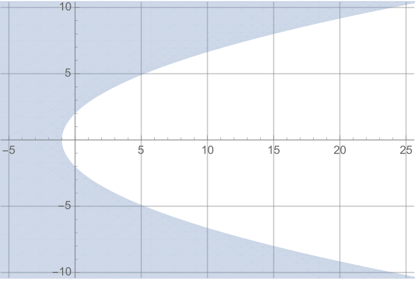
(a) Compact manifold case: $\Xi_{1}$

(b) Euclidean case: $\mathbb{C}\setminus[0,\infty)$

Figure 5. Spectral regions for which the uniform $L^{\frac{2d}{d+2}}$–$L^{\frac{2d}{d-2}}$ resolvent estimate holds.

Regions of spectral parameters where uniform resolvent estimate is allowed

Since we now have sharp resolvent estimates which depend on the spectral parameter $z$, it is possible, for each given $p,q$, to describe the region of $z$ for which the resolvent estimates are uniform.

The $L^{\frac{2d}{d+2}}(\mathbb{R}^{d})$–$L^{\frac{2d}{d-2}}(\mathbb{R}^{d})$ bound for $(-\Delta-z)^{-1}$ is uniform in $z\in\mathbb{C}\setminus[0,\infty)$ while the uniform estimate (1.16) on compact manifold holds only for $z\in\Xi_{\delta}$ (see Figure 5). Thus, we may reasonably expect that the bound $\|(-\Delta-z)^{-1}\|_{p\to q}$ behaves better on $\mathbb{R}^{d}$ than on compact manifolds. However, as is to be seen below, it is rather surprising that, for certain $p,q$, the bound for $\|(-\Delta-z)^{-1}\|_{p\to q}$ has a similar behavior with those on compact manifolds and the profile of the $z$-region where $\|(-\Delta-z)^{-1}\|_{p\to q}$ is uniformly bounded changes dramatically depending on the values of $p,q$.

For $p,q$ which satisfy $(1/p,1/q)\in\mathcal{R}_{1}\cup\big{(}\bigcup_{i=2}^{3}\widetilde{\mathcal{R}}_{i}\big{)}\cup\widetilde{\mathcal{R}}_{3}^{\prime}$, and $\ell>0$ we define the region $\mathcal{Z}_{p,q}(\ell)$ of spectral parameters by

$$\mathcal{Z}_{p,q}(\ell):=\{z\in\mathbb{C}\setminus[0,\infty):{\kappa}_{p,q}(z)\leq\ell\}.$$

For simplicity, let us focus on the case $\ell=1$, and describe roughly the typical shapes of $\mathcal{Z}_{p,q}(1)$. See Section 4.4 (and Figure 8 and Figure 9) for detailed description of $\mathcal{Z}_{p,q}(\ell)$ in terms of $p,q,d,$ and $\ell$.

• If $d\geq 3$ and $(1/p,1/q)\in(A,A^{\prime})$, then $\mathcal{Z}_{p,q}(1)=\mathbb{C}\setminus[0,\infty)$ (see Figure 5(b)).

• If $(1/p,1/q)\in\mathcal{R}_{1}$, and $1/p-1/q<2/d$, then $\mathcal{Z}_{p,q}(1)$ is given by removing the unit disk centered at zero from $\mathbb{C}\setminus[0,\infty)$ (see Figure 6(a)).

• If $(1/p,1/q)\in\widetilde{\mathcal{R}}_{2}$, then $\mathcal{Z}_{p,q}(1)$ basically have two different types. When $(p,q)\neq(2,2)$, $\mathcal{Z}_{p,q}(1)$ is the complex plane minus a neighborhood of $[0,\infty)$ which shrinks along the positive real line as $\mathop{\mathrm{Re}}z\to\infty$ (see Figure 6(b)). When $p=q=2$, $\mathcal{Z}_{2,2}(1)$ is the complex plane from which the $1$-neighborhood of $[0,\infty)$ is removed (see Figure 6(c)).

A remarkably interesting phenomenon occurs when $(1/p,1/q)\in\widetilde{\mathcal{R}}_{3}\cup\widetilde{\mathcal{R}}_{3}^{\prime}$. To describe this let us divide $\widetilde{\mathcal{R}}_{3}$ into the three subsets $\widetilde{\mathcal{R}}_{3,+}$, $\widetilde{\mathcal{R}}_{3,0}$, and $\widetilde{\mathcal{R}}_{3,-}$, given by

$$\widetilde{\mathcal{R}}_{3,\pm}:=\Big{\{}(x,y)\in\widetilde{\mathcal{R}}_{3}:\pm\Big{(}x+y-\frac{d-1}{d}\Big{)}>0\Big{\}},\quad\widetilde{\mathcal{R}}_{3,0}:=\Big{\{}(x,y)\in\widetilde{\mathcal{R}}_{3}:x+y-\frac{d-1}{d}=0\Big{\}}.$$

• If $(1/p,1/q)\in\widetilde{\mathcal{R}}_{3,+}\cup\widetilde{\mathcal{R}}_{3,+}^{\prime}$, $\mathcal{Z}_{p,q}(1)$ is similar type as in the case $(1/p,1/q)\in\widetilde{\mathcal{R}}_{2}\setminus\{H\}$ (see Figure 6(b)).

• If $(1/p,1/q)\in\widetilde{\mathcal{R}}_{3,0}\cup\widetilde{\mathcal{R}}_{3,0}^{\prime}$, we have $\mathcal{Z}_{p,q}(1)=\mathcal{Z}_{2,2}(1)$ (see Figure 6(c)).

• Let $(1/p,1/q)\in\widetilde{\mathcal{R}}_{3,-}\cup\widetilde{\mathcal{R}}_{3,-}^{\prime}$. If $1/p-1/q<2/d$, $\mathcal{Z}_{p,q}(1)$ is the complement (in $\mathbb{C}$) of a neighborhood of $[0,\infty)$ whose boundary becomes wider as $\mathop{\mathrm{Re}}z$ gets large (see Figure 6(d)). If $1/p-1/q=2/d$, then $\mathcal{Z}_{p,q}(1)=\{z\in\mathbb{C}\setminus\{0\}:\mathop{\mathrm{Re}}z\leq 0\}$.

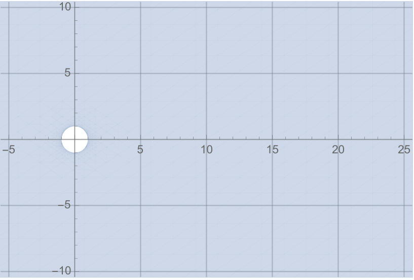
(a) $(\frac{1}{p},\frac{1}{q})\in\mathcal{R}_{1}\setminus(A,A^{\prime})$

(b) $(\frac{1}{p},\frac{1}{q})\in(\widetilde{\mathcal{R}}_{2}\setminus\{H\})\cup\widetilde{\mathcal{R}}_{3,+}\cup\widetilde{\mathcal{R}}_{3,+}^{\prime}$

(c) $(\frac{1}{p},\frac{1}{q})\in\{H\}\cup\widetilde{\mathcal{R}}_{3,0}\cup\widetilde{\mathcal{R}}_{3,0}^{\prime}$

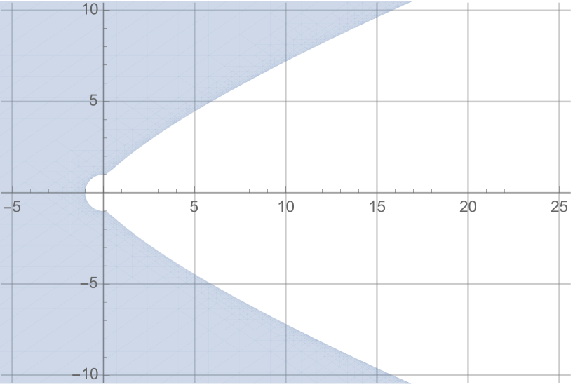
(d) $(\frac{1}{p},\frac{1}{q})\in\widetilde{\mathcal{R}}_{3,-}\cup\widetilde{\mathcal{R}}_{3,-}^{\prime}$

Figure 6. Some typical appearances of the spectral region $\mathcal{Z}_{p,q}(1)$ when $d\geq 3$ and $\frac{1}{p}-\frac{1}{q}<\frac{2}{d}$ .

Location of the eigenvalues of $-\Delta+V$

The sharp resolvent estimates (Theorem 1.4) can be used to specify the location of eigenvalues of non-self-adjoint Schrödinger operators $-\Delta+V$ acting in $L^{q}(\mathbb{R}^{d})$, $1\leq q\leq\infty$. As was shown in [17, 18], if $-\Delta+V$ acts in $L^{2}(\mathbb{R}^{d})$ one can use the Birman–Schwinger principle, but this is not the case when $-\Delta+V$ acts in $L^{q}(\mathbb{R}^{d})$, $q\neq 2$.

Corollary 1.5.

Let $(1/p,1/q)\in\mathcal{R}_{1}\cup\big{(}\bigcup_{i=2}^{3}\widetilde{\mathcal{R}}_{i}\big{)}\cup\widetilde{\mathcal{R}}_{3}^{\prime}$ and let $C>0$ be the constant which appears in (1.14). Fix a positive number $\ell>0$ (we choose $\ell\geq 1$ if $1/p-1/q=2/d$). Suppose that, for some $t\in(0,1)$,

(1.18) $$\|V\|_{L^{\frac{pq}{q-p}}(\mathbb{R}^{d})}\leq t(C\ell)^{-1}.$$

If $E\in\mathbb{C}\setminus[0,\infty)$ is an eigenvalue of $-\Delta+V$ acting in $L^{q}(\mathbb{R}^{d})$, then $E$ must lie in $\mathbb{C}\setminus\mathcal{Z}_{p,q}(\ell)$.

This is rather a direct consequence of Theorem 1.4. Let $u\in L^{q}(\mathbb{R}^{d})$ be an eigenfunction of $-\Delta+V$ with eigenvalue $E\in\mathbb{C}\setminus[0,\infty)$. If $E$ were contained in $\mathcal{Z}_{p,q}(\ell)$, Theorem 1.4 gives $\|(-\Delta-E)^{-1}\|_{p\to q}\leq C{\kappa}_{p,q}(E)\leq C\ell$. By Minkowski’s and Hölder’s inequalities, and (1.18) we have

$$\|u\|_{q}\leq C\ell\big{(}\|(-\Delta+V-E)u\|_{p}+\|Vu\|_{p}\big{)}\leq C\ell\|V\|_{\frac{pq}{q-p}}\|u\|_{q}\leq t\|u\|_{q},$$

which implies $u=0$ since $t<1$. This is contradiction, hence $E$ must be in $\mathbb{C}\setminus\mathcal{Z}_{p,q}(\ell)$.

Remark 3.

It is possible to formulate a statement which is analogous to the observation in [18, p. 220, Remark (1)]. For example, if $(1/p,1/q)\in\widetilde{\mathcal{R}}_{2}\cup\widetilde{\mathcal{R}}_{3,+}\cup\widetilde{\mathcal{R}}_{3,+}^{\prime}$, then for a sequence of eigenvalues $\{E_{j}\}$ of $-\Delta+V$ acting in $L^{q}(\mathbb{R}^{d})$ such that $\mathop{\mathrm{Re}}E_{j}\to\infty$ we have $\mathop{\mathrm{Im}}E_{j}\to 0$ provided that $\|V\|_{\frac{pq}{q-p}}$ is small enough. However, it does not seem to be likely that this phenomenon continues to be true for $p,q$ satisfying $(1/p,1/q)\in\big{(}\widetilde{\mathcal{R}}_{3,0}\cup\widetilde{\mathcal{R}}_{3,-}\big{)}\cup\big{(}\widetilde{\mathcal{R}}_{3,0}\cup\widetilde{\mathcal{R}}_{3,-}\big{)}^{\prime}$ and it would be interesting to ask whether there is a potential $V\in L^{\frac{pq}{q-p}}$ for which this kind of phenomenon fails.

Remark 4.

If $1/p-1/q=2/d$, and (1.18) is satisfied with some $\ell\geq 1$ and $t\in(0,1)$, then it follows from Corollary 1.5 that the Schrödinger operator $-\Delta+V$ acting in $L^{q}(\mathbb{R}^{d})$ does not have any eigenvalue of which real part is negative.

Sharp resolvent estimate for the fractional Laplacian

We also consider the sharp bound on $\|((-\Delta)^{\frac{s}{2}}-z)^{-1}\|_{p\to q}$, that is to say, the $L^{p}$–$L^{q}$ resolvent estimate for the fractional Laplacian $(-\Delta)^{\frac{s}{2}}$ which is defined by

$$(-\Delta)^{\frac{s}{2}}f(x)=\frac{1}{(2\pi)^{d}}\int_{\mathbb{R}^{d}}e^{ix\cdot\xi}|\xi|^{s}\widehat{f}(\xi)d\xi.$$

Uniform bounds on $\|((-\Delta)^{\frac{s}{2}}-z)^{-1}\|_{p\to q}$ for $p,q$ on certain range were obtained in Cuenin [14] and these bounds were used to study eigenvalues of the fractional Schrödinger operators with complex potentials. Later, uniform bounds up to the optimal range of $p,q$ were obtained by Huang, Yao, and Zheng [29]. We also obtain the sharp bounds on $\|((-\Delta)^{\frac{s}{2}}-z)^{-1}\|_{p\to q}$ for $p,q$ which are not contained in the uniform boundedness range. See Theorem 6.2.

Our method here is flexible and robust enough so that it is rather straightforward to extend our argument from the Laplacian to the fractional Laplacian. This allows us to obtain the sharp bounds on $((-\Delta)^{\frac{s}{2}}-z)^{-1}$ for $s\in(0,d)$, which include the results for the resolvent of the Laplacian. Furthermore, Proposition 1.3, Theorem 1.4, and Corollary 1.5, can also be generalized in the context of the fractional Laplacian $(-\Delta)^{\frac{s}{2}}$, $s>0$. There are also some new phenomena which do not appear in the study of the resolvent of the Laplacian. For example, if $s$ is small, the profile of the spectral parameter region where uniform bound is allowed never takes the form such as in Figure 6(b) (see Section 6 for details). However, we postpone discussions regrading the resolvent of the fractional Laplacian until the last section to keep the presentation simpler.

Organization of this paper

In Section 2, we review some properties of hypersurfaces of elliptic type, and the $L^{p}$–$L^{q}$ estimate for the Carleson–Sjölin type oscillatory integral operators. Then we obtain sharp estimates for the related multiplier operators of which frequency is localized. In Section 3, based on the results obtained in Section 2, we establish Proposition 2.4 which is the main ingredient for the proof of Theorem 1.4. In Section 4 we prove Theorem 1.4, and give descriptions in detail for various regions of spectral parameters $\mathcal{Z}_{p,q}(\ell)$ depending on $p$, $q$, $d$, and $\ell$. In Section 5 the proof of Proposition 1.1 and Proposition 1.3 is given. In Section 6 we obtain the sharp resolvent estimates for the fractional Laplacian $(-\Delta)^{\frac{s}{2}}$, $0<s<d$.

Notations

For positive numbers $A$ and $B$, $A\lesssim B$ means that there is a constant $C$ such that $A\leq CB$. We write $A\approx B$ if $A\lesssim B$ and $B\lesssim A$. Both $x\cdot y$ and $\langle x,y\rangle$ denote the Euclidean inner product of $x$ and $y$. For a function $f$ on $\mathbb{R}^{d}$

$$\mathcal{F}f(\xi)=\widehat{f}(\xi)=\int_{\mathbb{R}^{d}}f(x)e^{-ix\cdot\xi}dx,\qquad\mathcal{F}^{-1}f(\xi)=f^{\vee}(\xi)=(2\pi)^{-d}\widehat{f}(-\xi)$$

denote the Fourier and inverse Fourier transforms, respectively. We set $D=-i({\partial}/{\partial x_{1}},\cdots,{\partial}/{\partial x_{d}})$. For a bounded measurable function $m$, $m(D)f$ denotes the Fourier multiplier operator $(m\widehat{f}\,)^{\vee}$. For $p,q\in[1,\infty]$ we define $\|m(D)\|_{p\to q}:=\sup_{\|f\|_{p}\leq 1}\|m(D)f\|_{q}$. For any pair of subsets $A$, $B$ of the Euclidean spaces or the complex plane, we write $\operatorname{dist}(A,B):=\inf\{|x-y|:x\in A,\,y\in B\}$. For any rectangle $Q$ and a positive number $a$, $aQ$ is the rectangle whose side length is $a$ times that of $Q$ with same center as $Q$. $B_{d}(c,r)$ is the open ball in $\mathbb{R}^{d}$ centered at $c$ with radius $r$. If $A$ is a set $\chi_{A}$ is the characteristic function of $A$. We denote by $C_{0}^{\infty}(X)$ the class of smooth functions which are compactly supported in the set $X$. Throughout this paper, we fix an even function $\beta\in C^{\infty}_{0}(\mathbb{R})$ which is supported in the interval $[-9/8,-3/8]\cup[3/8,9/8]$ and satisfies $\sum_{j=-\infty}^{\infty}\beta(2^{-j}t)=1$ whenever $t\neq 0$. We also set $\beta_{0}=1-\sum_{j\geq 0}\beta(2^{-j}\,\cdot\,)\in C^{\infty}_{0}((-3/4,3/4))$. For a variable $x\in\mathbb{R}^{d}$ and a multi-index $\alpha\in\mathbb{N}_{0}^{d}$ we sometimes write $x=(x^{\prime},x_{d})\in\mathbb{R}^{d-1}\times\mathbb{R}$ and $\alpha=(\alpha^{\prime},\alpha_{d})\in\mathbb{N}_{0}^{d-1}\times\mathbb{N}_{0}$.

Acknowledgement

The authors were supported by NRF-2018R1A2B2006298. We would like to thank Ihyeok Seo and Younghun Hong for discussions on related issues, and the anonymous referees for various helpful comments.

2. Estimates for localized frequency

In this section we prove basic estimates which play important roles in obtaining our main result.

2.1. Oscillatory integral operator of Carleson–Sjölin type

Let $\lambda\geq 1$, $\mathfrak{a}\in C^{\infty}_{0}(\mathbb{R}^{d}\times\mathbb{R}^{d-1})$, $\Phi\in C^{\infty}(\mathbb{R}^{d}\times\mathbb{R}^{d-1})$, and let $T_{\lambda}[\Phi,\mathfrak{a}]$ be the operator defined by

$$T_{\lambda}[\Phi,\mathfrak{a}]f(x)=\int_{\mathbb{R}^{d-1}}e^{i\lambda\Phi(x,u)}\mathfrak{a}(x,u)f(u)du,\quad(x,u)\in\mathbb{R}^{d}\times\mathbb{R}^{d-1}.$$

Suppose that, for every $(x,u)\in\operatorname{supp}\mathfrak{a}$,

(2.1) $$\operatorname{rank}\big{(}\partial_{x}\partial_{u}\Phi(x,u)\big{)}=d-1.$$

We also assume that, for every $(x_{\circ},u_{\circ})\in\operatorname{supp}\mathfrak{a}$, if $v\in\mathbb{S}^{d-1}$ is the (unique up to sign) direction such that the function $u\to\langle v,\partial_{x}\Phi(x_{\circ},u)\rangle$ has a critical point at $u=u_{\circ}$, then

(2.2) $$\operatorname{rank}\left(\partial_{u}^{2}\langle v,\partial_{x}\Phi(x_{\circ},u)\rangle|_{u=u_{\circ}}\right)=d-1.$$

The operator $T_{\lambda}[\Phi,\mathfrak{a}]$ with $\Phi$ satisfying (2.1), (2.2) on $\operatorname{supp}\mathfrak{a}$ is called the Carleson–Sjölin type oscillatory integral operator which originated from the work of Carleson and Sjölin [11] for the study of the two dimensional Bochner–Riesz problem (also, see [44, pp. 60–70], [38]). Hörmander [27] proved

(2.3) $$\|T_{\lambda}[\Phi,\mathfrak{a}]f\|_{L^{q}(\mathbb{R}^{2})}\lesssim\lambda^{-2/q}\|f\|_{L^{p}(\mathbb{R})}$$

if $4<q\leq\infty$ and $3/q\leq 1-1/p$, and the range of $p,q$ for (2.3) is optimal. The following higher dimensional extension is due to Stein [45] (also, see [46, Chapter 9]).

Theorem 2.1.

Suppose $\Phi$ satisfies (2.1) and (2.2) on $\operatorname{supp}\mathfrak{a}$. Then, for $1\leq p,q\leq\infty$ satisfying $q\geq\frac{2(d+1)}{d-1}$ and $\frac{d+1}{q}\leq(d-1)(1-\frac{1}{p})$, the following estimate holds:

(2.4) $$\|T_{\lambda}[\Phi,\mathfrak{a}]f\|_{L^{q}(\mathbb{R}^{d})}\lesssim\lambda^{-d/q}\|f\|_{L^{p}(\mathbb{R}^{d-1})}.$$

Bourgain [5] showed that the estimate (2.4) under the conditions (2.1) and (2.2) generally fails if $q<\frac{2(d+1)}{d-1}$ when $d\geq 3$ is odd. However, in [36] one of the authors observed that in addition to (2.1), (2.2), if we assume that

(2.5) the surface $$u\to\partial_{x}\Phi(x,u) d-1$$ has nonzero principal curvatures of the same sign,

then the range of $p,q$ for which (2.4) holds can be enlarged to $q>\frac{2(d+2)}{d}$. For most recent developments see Bourgain and Guth [6] and Guth, Hickman and Iliopoulou [23]. These results are based on multilinear estimates due to Bennett, Carbery and Tao [3] and the method of polynomial partitioning due to Guth [22, 21]. We record here the recent sharp result due to Guth, Hickman and Iliopoulou [23].

Theorem 2.2.

Let $d\geq 2$ and suppose $\Phi$ satisfies (2.1), (2.2) and (2.5) on $\operatorname{supp}\mathfrak{a}$. Then, the estimate (2.4) holds whenever $p=q>p_{*}$, for $p_{*}$ given in (1.15). This is sharp (up to endpoint) in the sense that there are examples of Carleson–Sjölin type operators $T_{\lambda}[\Phi,\mathfrak{a}]$ with phase functions satisfying all of (2.1), (2.2) and (2.5) for which the estimate (2.4) with $p=q$ fails whenever $p<p_{*}$.

Remark 5.

The estimate (2.4) with $p=q$ in Theorem 2.2 is uniform under small smooth perturbation of the phase $\Phi$ and the amplitude $\mathfrak{a}$. In fact, the estimate (2.4) in [23] was obtained by running induction argument over a class of operators while the phase functions are properly normalized. See [23, Lemma 4.1, Definition 11.3]. Since small smooth perturbation of the phase functions are allowed within the class of operators, stability of the estimates follows.

2.2. Functions of elliptic type

Let $N\in\mathbb{N}$ and $\epsilon>0$. Let us set ${\mathbf{I}}=[-1,1]$. Following [49] and [37], we define ${\bf Ell}(N,\epsilon)$ as the class of $C^{N}$-functions $\psi:{\mathbf{I}}^{d-1}\to\mathbb{R}$ satisfying

• $\psi(0)=0$ and $\nabla\psi(0)=0$;

• Let $w(\xi^{\prime})=\psi(\xi^{\prime})-|\xi^{\prime}|^{2}/2$. Then

  (2.6) $$\sup_{\xi^{\prime}\in{\mathbf{I}}^{d-1}}\max_{0\leq|\alpha|\leq N}|\partial^{\alpha}w(\xi^{\prime})|\leq\epsilon.$$

Typically $N$ is chosen to be large and $\epsilon$ to be small. As was pointed out in [49], every convex smooth hypersurface with nonvanishing Gaussian curvature can be locally parametrized as graph of a function of elliptic type after a proper affine transformation.

For later use, we record here an approximate property of functions of elliptic type, which is an easy consequence of Taylor’s theorem. Let $H\psi$ denote the Hessian matrix of $\psi$.

Lemma 2.3.

Let $N$, $\epsilon$ be as above and $0<\rho\leq 2^{-1}$. For $\psi\in{\bf Ell}(N,\epsilon)$ and $c\in(2^{-1}{\mathbf{I}})^{d-1}$ set

(2.7) $$\psi_{c,\rho}(\xi^{\prime})=\rho^{-2}\big{(}\psi(\rho\xi^{\prime}+c)-\psi(c)-\rho\nabla\psi(c)\cdot\xi^{\prime}\big{)}.$$

Then, we have

(2.8) $$\sup_{(\xi^{\prime},c)\in{\mathbf{I}}^{d-1}\times(2^{-1}{\mathbf{I}})^{d-1}}\Big{|}\partial_{\xi^{\prime}}^{\alpha}\Big{(}\psi_{c,\rho}(\xi^{\prime})-\frac{1}{2}\langle H\psi(c)\xi^{\prime},\xi^{\prime}\rangle\Big{)}\Big{|}\leq\begin{cases}\,\frac{(d-1)^{3-|\alpha|}}{(3-|\alpha|)!}\rho\epsilon&\text{if}\quad 0\leq|\alpha|\leq 2,\\[4.0pt] \,\rho^{|\alpha|-2}\epsilon&\text{if}\quad 3\leq|\alpha|\leq N.\end{cases}$$

Moreover, there is a constant $\mathfrak{c}$, depending only on $d$, such that if $\psi\in{\bf Ell}(N,\epsilon)$, then, for all $c\in(2^{-1}{\mathbf{I}})^{d-1}$ and $0<\rho\leq 2^{-1}$, $\psi_{c,\rho}\in{\bf Ell}(N,\mathfrak{c}\epsilon)$.

Proof.

Clearly $\psi_{c,\rho}(0)=0$ and $\nabla\psi_{c,\rho}(0)=0$. Let $|\xi^{\prime}|_{1}:=\sum_{k=1}^{d-1}|\xi_{k}|$. By Taylor’s theorem we have for $(\xi^{\prime},c)\in{\mathbf{I}}^{d-1}\times(2^{-1}{\mathbf{I}})^{d-1}$ that

$$\Big{|}\psi_{c,\rho}(\xi^{\prime})-\frac{1}{2}\langle H\psi(c)\xi^{\prime},\xi^{\prime}\rangle\Big{|}\leq\frac{|\xi^{\prime}|_{1}^{3}}{3!}\sup_{|\alpha|=3,\,0\leq t\leq 1}\left|\rho(\partial^{\alpha}\psi)(\rho t\xi^{\prime}+c)\right|\leq\frac{|\xi^{\prime}|_{1}^{3}}{3!}\rho\epsilon.$$

The second inequality follows from (2.6) since $\rho t\xi^{\prime}+c\in{\mathbf{I}}^{d-1}$ whenever $(\xi^{\prime},c)\in{\mathbf{I}}^{d-1}\times(2^{-1}{\mathbf{I}})^{d-1}$, $0<\rho\leq 2^{-1}$ and $0\leq t\leq 1$. Similarly, using Taylor’s theorem and (2.6) we also have

$$\Big{|}\partial_{\xi^{\prime}}^{\alpha}\Big{(}\psi_{c,\rho}(\xi^{\prime})-\frac{1}{2}\langle H\psi(c)\xi^{\prime},\xi^{\prime}\rangle\Big{)}\Big{|}\leq\begin{cases}\frac{\rho\epsilon}{2!}|\xi^{\prime}|_{1}^{2}&\text{if}\quad|\alpha|=1,\\[4.0pt] \rho\epsilon|\xi^{\prime}|_{1}&\text{if}\quad|\alpha|=2.\end{cases}$$

If $|\alpha|\geq 3$, then $\partial_{\xi^{\prime}}^{\alpha}\big{(}\psi_{c,\rho}(\xi^{\prime})-\frac{1}{2}\langle H\psi(c)\xi^{\prime},\xi^{\prime}\rangle\big{)}=\rho^{|\alpha|-2}(\partial^{\alpha}\psi)(\rho\xi^{\prime}+c)$. Hence we have (2.8). The second assertion follows immediately from (2.6), (2.8) and comparing $\langle H\psi(c)\xi^{\prime},\xi^{\prime}\rangle$ with $|\xi^{\prime}|^{2}$. ∎

2.3. Estimates for the operator with localized frequency

To obtain the sharp bound (1.14), the case in which $|z|\approx 1$, $\mathop{\mathrm{Re}}z>0$, and $|\mathop{\mathrm{Im}}z|\ll 1$ is most important (see Section 4.1 below). In this case, the corresponding Fourier multiplier carries most of its mass near the sphere $S_{z}:=\{\xi\in\mathbb{R}^{d}:|\xi|=\sqrt{\mathop{\mathrm{Re}}z}\}$, where $\sqrt{\mathop{\mathrm{Re}}z}\approx 1$. Since $S_{z}$ is compact and convex with non-vanishing curvature, using finite decomposition and affine transformations, we can regard $S_{z}$ as a finite union of graphs of functions of elliptic type. Such operations do not have significant effect on the estimate (1.14) except for a minor change of the multiplicative constant $C$.

Now, by a dyadic decomposition (away from the graph of a function $\psi(\xi^{\prime})$ of elliptic type) in the Fourier side, we need to obtain the sharp bounds for the multiplier operators of which Fourier transform is supported in a $\delta$-neighborhood of the surface $\xi_{d}=\psi(\xi^{\prime})$.

For $b>0$, let us set

$${{\bf Mul}({N},b)}=\{m\in C^{N}(\mathbb{R}^{d}):2^{-1}\leq|m|\leq 2,\ |\partial^{\alpha}m|\leq b,\ 1\leq|\alpha|\leq{N}\}.$$

Let $0<\delta\leq 1$, $\lambda\geq 1$ and $\delta\lambda\leq 1/{10}$, and let $\varphi\in C^{\infty}(\mathbb{R})$. For $\psi\in{{\bf Ell}(N,\epsilon)}$ and $m\in{{\bf Mul}({N},b)}$ we set

(2.9) $$\mathfrak{M}_{\delta}(\xi):=\varphi\Big{(}\frac{m(\xi)(\xi_{d}-\psi(\xi^{\prime}))}{\delta}\Big{)}\beta_{0}\Big{(}\frac{m(\xi)(\xi_{d}-\psi(\xi^{\prime}))}{\delta}\Big{)}\chi_{0}(\xi),$$

(2.10) $$\mathfrak{M}_{\delta,\lambda}(\xi):=\varphi\Big{(}\frac{m(\xi)(\xi_{d}-\psi(\xi^{\prime}))}{\delta}\Big{)}\beta\Big{(}\frac{m(\xi)(\xi_{d}-\psi(\xi^{\prime}))}{\delta\lambda}\Big{)}\chi_{0}(\xi),$$

where $\chi_{0}\in C^{\infty}_{0}(2^{-1}{\mathbf{I}}^{d})$. A particular example of $\varphi$ is the function $\varphi(t)=(2t\pm i)^{-1}$. In the proof of Theorem 1.4 (Section 4.3) $\psi$ parametrizes the surface given by a part of the sphere which is deformed under parabolic rescaling. By the additional $m$ we may perturb the multipliers $\mathfrak{M}_{\delta}$ and $\mathfrak{M}_{\delta,\lambda}$, so this allows us to handle other classes of operators which are given by multipliers with similar structure.

The following provide sharp estimates for $\mathfrak{M}_{\delta}(D)$ and $\mathfrak{M}_{\delta,\lambda}(D)$ and these are most important ingredients in proving Theorem 1.4. For its application, see Section 4.3 (especially (4.13)) and the proof of Theorem 2.13.

Proposition 2.4.

Let $b>0$ and suppose that, for $k\geq 0$,

(2.11) $$\Big{|}\Big{(}\frac{d}{dt}\Big{)}^{k}\varphi(t)\Big{|}\leq C_{k}t^{-k-1},\quad|t|\geq 1.$$

Then, for $p,q$ satisfying $\frac{1}{q}=\frac{d-1}{d+1}(1-\frac{1}{p})$ and $q_{\circ}<q\leq\frac{2(d+1)}{d-1}$, there exist $N$ and $\epsilon>0$ such that the following hold uniformly provided that $\psi\in{\bf Ell}(N,\epsilon)$ and $m\in{{\bf Mul}({N},b)}$:

(2.12) $$\left\|\mathfrak{M}_{\delta}(D)f\right\|_{L^{q}(\mathbb{R}^{d})}\leq C\delta^{\frac{1-d}{2}+\frac{d}{p}}\|f\|_{L^{p}(\mathbb{R}^{d})},$$

(2.13) $$\left\|\mathfrak{M}_{\delta,\lambda}(D)f\right\|_{L^{q}(\mathbb{R}^{d})}\leq C\lambda^{-1}(\delta\lambda)^{\frac{1-d}{2}+\frac{d}{p}}\|f\|_{L^{p}(\mathbb{R}^{d})}.$$

Here the constant $C$ may depend on $b$, $d$, $p$, $q$, $N$, $\epsilon$, $\varphi$ and $\chi_{0}$, but is independent of $\delta$, $\lambda$, $m$, $\psi$ and $f$.

Remark 6.

Similar estimates were obtained in [12, Proposition 2.4]. However, there are differences which need to be mentioned. Firstly, the function $\phi\in\mathcal{S}(\mathbb{R})$ in [12, Proposition 2.4] is assumed to have the special cancellation property $\operatorname{supp}\widehat{\phi}=\{t\in\mathbb{R}:|t|\approx 1\}$ which was crucial in obtaining the sharp estimate, whereas we do not need such extra assumption in Proposition 2.4. This is necessary for the proof of Theorem 1.4. Unlike [12] the associated multipliers $(|\xi|^{2}-z)^{-1}$ are not homogeneous, so we cannot decompose them in such a nice way as in [12, Lemma 2.1] (also, see [30, Section 2.1]). Secondly, we allow smooth perturbation of $m$ in (2.9) and (2.10) with $m$ satisfying $|m|\approx 1$. Lastly, the estimates (2.12) and (2.13) hold on a wider range of $p,q$ than that of the estimate in [12, Proposition 2.4].

We postpone the proof of Proposition 2.4 until the next section. For the rest of this section we present results which will be used for the proof of Proposition 2.4.

2.4. $L^{p}$ boundedness of multiplier operators

In this section, we obtain sharp $L^{p}$ estimates for the multiplier operators $\mathfrak{M}_{\delta}(D)$ and $\mathfrak{M}_{\delta,\lambda}(D)$ which are consequences of Theorem 2.2. We work with $\mathfrak{M}_{\delta,\lambda}(D)$ only, since the same argument also works for $\mathfrak{M}_{\delta}(D)$. In what follows all of the $L^{p}$ estimates are uniform in $\psi\in{\bf Ell}(N,\epsilon)$, $m\in{{\bf Mul}({N},b)}$, provided that $N$ is sufficiently large and $\epsilon$ is sufficiently small.

Proposition 2.5.

Let $b$, $\chi_{0}$, $\delta$, $\lambda$ and $\varphi$ be as in Proposition 2.4, and suppose that $p_{*}<p\leq\infty$. Then there exist a large $N>0$, a small $\epsilon>0$ and a constant $C>0$ such that

$$\|\mathfrak{M}_{\delta}(D)f\|_{L^{p}(\mathbb{R}^{d})} \leq C\delta^{\frac{d}{p}-\frac{d-1}{2}}\|f\|_{L^{p}(\mathbb{R}^{d})},$$

(2.14) $$\|\mathfrak{M}_{\delta,\lambda}(D)f\|_{L^{p}(\mathbb{R}^{d})} \leq C\lambda^{-1}(\delta\lambda)^{\frac{d}{p}-\frac{d-1}{2}}\|f\|_{L^{p}(\mathbb{R}^{d})},$$

where the constants $C$ are independent of $\delta$, $\lambda$, $\psi\in{\bf Ell}(N,\epsilon)$ and $m\in{{\bf Mul}({N},b)}$.

We will achieve this by making use of Theorem 2.2. For this purpose we need to compute the kernel $K_{\delta,\lambda}$ of the operator $\mathfrak{M}_{\delta,\lambda}(D)$.

Remark 7.

To begin with, we readjust the cutoff functions $\chi_{0}$ in (2.10) of which role is not so significant for the overall estimates. We may regard $\chi_{0}\widehat{f}$ as if it is $\widehat{f}$ (note that $\|\mathcal{F}^{-1}(\chi_{0}\widehat{f}\,)\|_{p}\lesssim\|f\|_{p}$ if $\chi_{0}\in C_{0}^{\infty}$). We may also introduce a new cutoff function $\chi^{\prime}$ whenever $\chi_{0}\chi^{\prime}=\chi_{0}$ and replace $\widehat{f}$ with $\chi^{\prime}\widehat{f}$. By decomposing (with a suitable partition of unity) $\chi_{0}$ into finitely many cutoff functions with smaller support (of diameter $\lesssim\epsilon_{0}$) we may assume $\chi_{0}$ is supported in a small neighborhood near the surface $\xi_{d}=\psi(\xi^{\prime})$. Otherwise, the contribution is negligible. In fact, the associated kernel has a bounded $L^{1}$-norm as can be seen easily by a straightforward kernel estimate. Let $\xi_{0}=(c,\psi(c))$ and suppose $\chi_{0}$ is supported in $B_{d}(\xi_{0},\epsilon_{0})$ for a fixed $\epsilon_{0}$. Then, for $0<\rho\leq 2^{-1}$, we may use the harmless affine transform

(2.15) $$\xi\to L_{c,\rho}(\xi)=\big{(}\rho\xi^{\prime}+c,\,\rho^{2}\xi_{d}+\psi(c)+\rho\nabla\psi(c)\cdot\xi^{\prime}\big{)}$$

to write

(2.16) $$\mathfrak{M}_{\delta,\lambda}(L_{c,\rho}(\xi))=\varphi\Big{(}\frac{m(L_{c,\rho}\xi)(\xi_{d}-\psi_{c,\rho}(\xi^{\prime}))}{\rho^{-2}\delta}\Big{)}\beta\Big{(}\frac{m(L_{c,\rho}\xi)(\xi_{d}-\psi_{c,\rho}(\xi^{\prime}))}{\rho^{-2}\delta\lambda}\Big{)}\chi_{0}(L_{c,\rho}\xi).$$

By Lemma 2.3 $\psi_{c,\rho}\in{\bf Ell}(N,\mathfrak{c}\epsilon)$. Also, $m\circ L_{c,\rho}\in{{\bf Mul}(N,Cb)}$ for some $C>0$. Thus we may regard this as the same multiplier given by (2.10) by simply replacing $\rho^{-2}\delta$, $m\circ L_{c,\rho}$ and $\psi_{c,\rho}$ with $\delta$, $m$ and $\psi$, respectively. Hence taking $\epsilon_{0}$ small enough and $\rho=\epsilon_{0}2^{7}$, after a simple manipulation (discarding the part of multiplier which is away from the surface) we may assume the cutoff function takes the form

$$\chi_{0}(\xi)=\chi(\xi^{\prime})\chi_{1}(\xi_{d}-\psi(\xi^{\prime}))$$

and $\chi\in C_{0}^{\infty}(B_{d-1}(0,2^{-7}))$ and $\chi_{1}\in C^{\infty}_{0}((-2^{-7},2^{-7}))$.

Before we prove (2.14) rigorously, we explain the idea behind our proof with a simplified multiplier. This will help the reader to understand the detailed (but technical) proof below in this section. Let us assume that $m=1$, $\varphi(t)=1/t$, $\psi(\xi^{\prime})=\frac{1}{2}|\xi^{\prime}|^{2}$ and $\chi_{0}(\xi)=\chi(\xi^{\prime})\chi_{1}(\xi_{d}-\psi(\xi^{\prime}))$. Then the multiplier takes the simpler form

$$\mathfrak{M}_{\delta,\lambda}(\xi)=\frac{1}{\lambda}b\Big{(}\frac{\xi_{d}-\psi(\xi^{\prime})}{\delta\lambda}\Big{)}\chi(\xi^{\prime})\chi_{1}(\xi_{d}-\psi(\xi^{\prime})),$$

where $b(t)=|t|^{-1}\beta(t)$. By the stationary phase method $K_{\delta,\lambda}(x):=\mathcal{F}^{-1}(\mathfrak{M}_{\delta,\lambda})(x)$ “approximately” equals

$$\lambda^{-1}|x_{d}|^{-\frac{d-1}{2}}e^{-i\frac{|x^{\prime}|^{2}}{2x_{d}}}\int e^{ix_{d}\xi_{d}}b(\xi_{d}/\delta\lambda)\chi_{1}(\xi_{d})d\xi_{d}$$

for $|x_{d}|\gtrsim 1$ and $|x^{\prime}|\lesssim|x_{d}|$. We dyadically decompose this kernel along $x_{d}$:

$$\sum_{l=1}^{\infty}\lambda^{-1}\beta(2^{-l}x_{d})|x_{d}|^{-\frac{d-1}{2}}e^{-i\frac{|x^{\prime}|^{2}}{2x_{d}}}\int e^{ix_{d}\xi_{d}}b(\xi_{d}/\delta\lambda)\chi_{1}(\xi_{d})d\xi_{d}=:\sum_{l=1}^{\infty}K_{\delta,\lambda,l}(x).$$

Now the matter reduces to obtaining

(2.17) $$\|2^{dl}K_{\delta,\lambda,l}(2^{l}\,\cdot\,)*f\|_{p}\lesssim 2^{(\frac{d+1}{2}-\frac{d}{p})l}\delta(1+2^{l}\delta\lambda)^{-M}\|f\|_{p},$$

because summation over $l$ gives the desired bound. Note that

$$2^{dl}K_{\delta,\lambda,l}(2^{l}\,\cdot\,)*f(x)=\lambda^{-1}2^{\frac{(d+1)l}{2}}\int e^{-i2^{l}\frac{|x^{\prime}-y^{\prime}|^{2}}{2|x_{d}-y_{d}|}}a_{\delta,\lambda,l}(x_{d}-y_{d})f(y)dy,$$

where $a_{\delta,\lambda,l}(x_{d}-y_{d})=\beta(x_{d}-y_{d})|x_{d}-y_{d}|^{-\frac{d-1}{2}}\int e^{i2^{l}(x_{d}-y_{d})\xi_{d}}b(\xi_{d}/\delta\lambda)\chi_{1}(\xi_{d})d\xi_{d}$. Application of the oscillatory integral estimate (Theorem 2.2) gives (2.17). Of course this is an oversimplification. We provide detailed argument in what follows.

By Remark 7 and change of variables $(\xi^{\prime},\xi_{d})\to(\xi^{\prime},\xi_{d}+\psi(\xi^{\prime}))$ we may write

(2.18) $$K_{\delta,\lambda}(x):=\mathcal{F}^{-1}(\mathfrak{M}_{\delta,\lambda})(x)=\frac{1}{2\pi}\int e^{ix_{d}\xi_{d}}\chi_{1}(\xi_{d})I_{\psi}(x;\xi_{d})\,d\xi_{d},$$

where

$$I_{\psi}(x;\xi_{d})=\frac{1}{(2\pi)^{d-1}}\int e^{i(x^{\prime}\cdot\xi^{\prime}+x_{d}\psi(\xi^{\prime}))}\varphi\Big{(}\frac{\widetilde{m}(\xi)\xi_{d}}{\delta}\Big{)}\beta\Big{(}\frac{\widetilde{m}(\xi)\xi_{d}}{\delta\lambda}\Big{)}\chi(\xi^{\prime})d\xi^{\prime}$$

and $\widetilde{m}(\xi)=m(\xi^{\prime},\xi_{d}+\psi(\xi^{\prime}))$. $\widetilde{m}$ still enjoys the same property as $m$ in Proposition 2.4, that is to say, $\widetilde{m}\in{\bf Mul}(N,Cb)$ for some $C>0$. For simplicity we put

(2.19) $$A_{\delta,\lambda}(\xi):=\varphi\Big{(}\frac{\widetilde{m}(\xi)\xi_{d}}{\delta}\Big{)}\beta\Big{(}\frac{\widetilde{m}(\xi)\xi_{d}}{\delta\lambda}\Big{)}\chi(\xi^{\prime}).$$

Let us collect some bounds for the functions $A_{\delta,\lambda}$ and their differentials which will be useful later when we show Proposition 2.5.

Lemma 2.6.

Let $0<\delta\leq\delta\lambda\leq 1$, $b>0$ and let $\psi\in{\bf Ell}(N,\epsilon)$, $m\in{{\bf Mul}({N},b)}$. Then, for every $(d-1)$-dimensional multi-index $\vartheta\in\mathbb{N}_{0}^{d-1}$ with $|\vartheta|\leq N$, we have

(2.20) $$\sup_{\xi}\big{|}\partial_{\xi^{\prime}}^{\vartheta}A_{\delta,\lambda}(\xi)\big{|}\leq C_{\vartheta}\lambda^{-1}$$

uniformly in $\delta$, $\lambda$, $\psi\in{\bf Ell}(N,\epsilon)$ and $m\in{{\bf Mul}({N},b)}$. More generally, for every $d$-dimensional multi-index $\alpha=(\alpha^{\prime},\alpha_{d})\in\mathbb{N}_{0}^{d-1}\times\mathbb{N}$ and every $\vartheta\in\mathbb{N}_{0}^{d-1}$ such that $|\alpha|+|\vartheta|\leq N$, we have

(2.21) $$\sup_{\xi}\big{|}\partial_{\xi^{\prime}}^{\alpha^{\prime}}\partial_{\xi_{d}}^{\alpha_{d}}\big{(}(\xi_{d})^{\ell}\partial_{\xi^{\prime}}^{\vartheta}A_{\delta,\lambda}(\xi)\big{)}\big{|}\leq C_{\alpha,\vartheta}\lambda^{-1}(\delta\lambda)^{-\alpha_{d}+\ell}$$

with $C_{\alpha,\vartheta}$ independent of $\delta$, $\lambda$, $m$ and $\psi$.

Proof.

For every $k\in\mathbb{N}_{0}$ note that $\beta^{(k)}\big{(}\frac{\widetilde{m}(\xi)\xi_{d}}{\delta\lambda}\big{)}\neq 0$ only if $|\xi_{d}|\approx\delta\lambda$ since $|\widetilde{m}|\approx 1$. Hence for every $\vartheta\in\mathbb{N}_{0}^{d-1}$ with $0\leq|\vartheta|\leq N$ it is easy to see that $\operatorname{supp}\partial_{\xi^{\prime}}^{\vartheta}A_{\delta,\lambda}$ is contained in the set $\{\xi:|\xi_{d}|\approx\delta\lambda\}$ and that

(2.22) $$\sup_{\xi}\Big{|}\partial_{\xi^{\prime}}^{\vartheta}\Big{(}\beta\Big{(}\frac{\widetilde{m}(\xi)\xi_{d}}{\delta\lambda}\Big{)}\Big{)}\Big{|}\leq C_{\vartheta}$$

with $C_{\vartheta}$ independent of $\delta$, $\lambda$, $m$ and $\psi$. Also, for $0\leq|\vartheta|\leq N$,

$$\sup_{\xi}\Big{|}\partial_{\xi^{\prime}}^{\vartheta}\Big{(}\varphi\Big{(}\frac{\widetilde{m}(\xi)\xi_{d}}{\delta}\Big{)}\Big{)}\Big{|}\lesssim\sum_{k=0}^{|\vartheta|}\sup_{\xi}\Big{|}\varphi^{(k)}\Big{(}\frac{\widetilde{m}(\xi)\xi_{d}}{\delta}\Big{)}\Big{(}\frac{\xi_{d}}{\delta}\Big{)}^{k}\Big{|},$$

where the implicit constant is independent of $\delta$, $\lambda$, $m$ and $\psi$. Since $|\widetilde{m}|\approx 1$ and $|\xi_{d}|\approx\lambda\delta$ on $\operatorname{supp}A_{\delta,\lambda}$, by (2.11) we see that

(2.23) $$\sup_{\xi^{\prime}\in\operatorname{supp}\chi,\,|\xi_{d}|\approx\delta\lambda}\Big{|}\partial_{\xi^{\prime}}^{\vartheta}\Big{(}\varphi\Big{(}\frac{\widetilde{m}(\xi)\xi_{d}}{\delta}\Big{)}\Big{)}\Big{|}\leq C_{\vartheta}\lambda^{-1}.$$

By combining (2.22) and (2.23) it is easy to see (2.20).

For the proof of (2.21) we first consider the case $\alpha^{\prime}=\vartheta=0$. Note that $\partial_{\xi_{d}}^{\alpha_{d}}\big{(}(\xi_{d})^{\ell}A_{\delta,\lambda}\big{)}$ is given by a linear combination of $(\xi_{d})^{\ell-n}\partial_{\xi_{d}}^{\alpha_{d}-n}A_{\delta,\lambda}$ and $\partial_{\xi_{d}}^{\alpha_{d}-n}A_{\delta,\lambda}$ is also a linear combination of

$$\delta^{-\nu}(\lambda\delta)^{-\mu}\chi_{\mu,\nu}(\xi)\varphi^{(\nu)}\Big{(}\frac{\widetilde{m}(\xi)\xi_{d}}{\delta}\Big{)}\beta^{(\mu)}\Big{(}\frac{\widetilde{m}(\xi)\xi_{d}}{\delta\lambda}\Big{)},\quad\mu+\nu\leq\alpha_{d}-n.$$

Here $\chi_{\mu,\nu}$ is a smooth function with bounded derivatives. Since $|\xi_{d}|\approx\lambda\delta$ on $\operatorname{supp}A_{\delta,\lambda}$, we deduce the desired bound (2.21) by (2.11). For the general cases one can routinely repeat the same argument keeping in mind that $\partial_{\xi^{\prime}}^{\alpha^{\prime}}$ or $\partial_{\xi^{\prime}}^{\vartheta}$ behaves almost similarly as in (2.20) on $\operatorname{supp}A_{\delta,\lambda}$. So, we omit the detail. ∎

We now obtain the asymptotic for the function $I_{\psi}(\,\cdot\,,\xi_{d})$. Since $\psi\in{\bf Ell}(N,\epsilon)$, $\nabla\psi(0)=0$ and $\nabla\psi(\xi^{\prime})=\xi^{\prime}+O(\epsilon)$ for $\xi^{\prime}\in{\mathbf{I}}^{d-1}$. Thus, by the inverse function theorem we see that there exist neighborhoods $U$, $V$ of the origin and a unique diffeomorphism $g:U\to V$ such that $g(0)=0$ and

(2.24) $$t^{\prime}+\nabla\psi(g(t^{\prime}))=0.$$

If we take $\epsilon$ sufficiently small, we may assume that $U\supset B_{d-1}(0,1/2)$. In fact, $(g(t^{\prime}),\psi\circ g(t^{\prime}))$ is the unique point on the graph $\mathcal{G}(\psi):=\{(\xi^{\prime},\psi(\xi^{\prime})):\xi^{\prime}\in\operatorname{supp}\chi\}$ at which the normal vector is parallel to $(t^{\prime},1)$. We denote by ${\bf K}(\xi)$ the Gaussian curvature of the surface $\mathcal{G}(\psi)$ at point $\xi=(\xi^{\prime},\psi(\xi^{\prime}))$ and by ${\bf J}g$ the Jacobian matrix of the diffeomorphism $g$. Direct differentiation of the equation (2.24) gives

(2.25) $$((H\psi)\circ g)\cdot{\bf J}g=-I_{d-1}.$$

Lemma 2.7.

Let $0<\delta\leq\delta\lambda\lesssim 1$. Suppose that $N$ (resp., $\epsilon$) is large (resp., small) enough so that for every $\psi\in{\bf Ell}(N,\epsilon)$, the aforementioned diffeomorphism $g:U\supset B_{d-1}(0,1/2)\to V$ exists. Then the following hold.

$(\mathrm{I})$ If $|x_{d}|\geq 1/2$ and $2^{5}|x^{\prime}|\leq|x_{d}|$, then for every $M\in\mathbb{N}$ satisfying $2M\leq N$ we have

(2.26) $$I_{\psi}(x;\tau)=\frac{c_{d}}{\sqrt{|{\bf K}|}}e^{i(x^{\prime}\cdot g(\frac{x^{\prime}}{x_{d}})+x_{d}\psi\circ g(\frac{x^{\prime}}{x_{d}}))}\sum_{j=0}^{M-1}\mathcal{D}_{j}A_{\delta,\lambda}(\xi^{\prime},\tau)\Big{|}_{\xi^{\prime}=g(\frac{x^{\prime}}{x_{d}})}|x_{d}|^{-\frac{d-1}{2}-j}+\mathcal{E}_{\delta,\lambda,M}(x;\tau),$$

where $c_{d}$ is a constant depending only on $d$, $|{\bf K}|=\big{|}{\bf K}\big{(}g(\frac{x^{\prime}}{x_{d}}),\,\psi\circ g(\frac{x^{\prime}}{x_{d}})\big{)}\big{|}\approx 1$, $\mathcal{D}_{0}A_{\delta,\lambda}=A_{\delta,\lambda}$ and, for each $j\geq 1$, $\mathcal{D}_{j}$ is a differential operator in $\xi^{\prime}$ of order $2j$ whose coefficients vary smoothly depending on $\big{(}\partial_{\xi^{\prime}}^{\alpha}\psi\big{)}\circ g\big{(}\frac{x^{\prime}}{x_{d}}\big{)},$ $2\leq|\alpha|\leq 2j+2$. For $\mathcal{E}_{\delta,\lambda,M}(x;\tau)$ we have the estimate

(2.27) $$\big{|}\mathcal{E}_{\delta,\lambda,M}(x;\tau)\big{|}\leq C|x_{d}|^{-M}\sum_{|\alpha|\leq 2M}\sup_{(\xi^{\prime},\tau)}\big{|}\partial_{\xi^{\prime}}^{\alpha}A_{\delta,\lambda}(\xi^{\prime},\tau)\big{|}\leq C^{\prime}|x_{d}|^{-M}\lambda^{-1}$$

with $C^{\prime}$ independent of $\delta$, $\lambda$, $m$ and $\psi$.

$(\mathrm{I}\!\mathrm{I})$ On the other hand, if $2^{6}|x^{\prime}|\geq|x_{d}|$ or $|x_{d}|\leq 2$, then for every $0\leq M\leq N$ there exists a constant $C_{M}$, independent of $\delta$, $\lambda$, $m$ and $\psi$, such that

(2.28) $$|I_{\psi}(x;\tau)|\leq C_{M}\lambda^{-1}(1+|x|)^{-M}.$$

Proof.

The asymptotic expansion (2.26) in $(\mathrm{I})$ is a consequence of the stationary phase method. For its proof we refer the reader to [28, Theorem 7.7.5 and Theorem 7.7.6]. In (2.27) the uniformity of $C^{\prime}$ in $\delta$, $\lambda$, $m$ and $\psi$ follows from Lemma 2.6.

For the second statement $(\mathrm{I}\!\mathrm{I})$ we use integration by parts. Since $\operatorname{supp}\chi\subset B_{d-1}(0,2^{-7})$ and $|\nabla\psi(\xi^{\prime})|\leq(1+c\epsilon)|\xi^{\prime}|$, it is easy to observe that, if $\epsilon$ is sufficiently small and $2^{6}|x^{\prime}|\geq|x_{d}|$,

$$|\nabla_{\xi^{\prime}}(x^{\prime}\cdot\xi^{\prime}+x_{d}\psi(\xi^{\prime}))|\geq|x^{\prime}|(1-2^{6}|\nabla\psi(\xi^{\prime})|)\gtrsim|x^{\prime}|.$$

If $|x_{d}|\leq 2$ the same estimate also holds with $|x^{\prime}|\geq 1$. Hence (2.28) follows from integration by parts in $\xi^{\prime}$ together with (2.20) in Lemma 2.6. ∎

Now we prove (2.14) by combining Theorem 2.2 and Lemma 2.7.

Proof of (2.14).

Let $\widetilde{\chi}$ be a smooth function on $\mathbb{R}$ supported in the interval $(-2^{-5},2^{-5})$ and equal to $1$ on $(-2^{-6},2^{-6})$. We break the kernel $K_{\delta,\lambda}$ as follows:

$$K_{\delta,\lambda}(x)=K_{\delta,\lambda,0}(x)+\sum_{l=1}^{\infty}K_{\delta,\lambda,l}(x),$$

where

$$K_{\delta,\lambda,l}(x)=\widetilde{\chi}\Big{(}\frac{|x^{\prime}|}{x_{d}}\Big{)}\beta(2^{-l}x_{d})K_{\delta,\lambda}(x)$$

for $l\in\mathbb{N}$. So, the function $K_{\delta,\lambda,0}$ is supported on the set $R:=\{x:2^{6}|x^{\prime}|\geq|x_{d}|\}\cup\{x:|x_{d}|\leq 2\}$, and it follows from (2.28) ($(\mathrm{I}\!\mathrm{I})$ in Lemma 2.7) that

$$|K_{\delta,\lambda,0}(x)|\leq C_{M}\lambda^{-1}(1+|x|)^{-M}$$

for any $0\leq M\leq N$, uniformly in $\delta$, $\lambda$. Since $\|K_{\delta,\lambda,0}\|_{1}\lesssim\lambda^{-1}$, the operator $f\to K_{\delta,\lambda,0}*f$ admits much better estimate than (2.14) since $p>p_{*}\geq\frac{2d}{d-1}$ and $\delta\lambda\lesssim 1$. Therefore it suffices to prove that

(2.29) $$\sum_{l=1}^{\infty}\|K_{\delta,\lambda,l}*f\|_{p}\leq C\lambda^{-1}(\delta\lambda)^{\frac{d}{p}-\frac{d-1}{2}}\|f\|_{p}.$$

To show this we need the asymptotic (2.26) for $I_{\psi}(\,\cdot\,;\xi_{d})$, which is to be combined with (2.18). Fixing $M\leq 2N$ large enough, it is enough to handle the finite summation in (2.26) since the contribution from the error term $\mathcal{E}_{\delta,\lambda,M}$ in (2.27) is at most $\lambda^{-1}$. In fact, since $(K_{\delta,\lambda}-K_{\delta,\lambda,0})(x)\neq 0$ only if $|x^{\prime}|\lesssim|x_{d}|$, if we set $K_{err}(x)=\frac{1}{2\pi}\int e^{ix_{d}\xi_{d}}\chi_{1}(\xi_{d})\mathcal{E}_{\delta,\lambda,M}(x,\xi_{d})d\xi_{d}$, it follows from (2.27) that $\|K_{err}\|_{1}\lesssim\lambda^{-1}$. Thus, the contribution from the first term in (2.26) is most significant and it suffices to prove (2.29) by replacing $K_{\delta,\lambda,l}$ with

(2.30) $$\widetilde{K}_{\delta,\lambda,l}(x) =\widetilde{\chi}\Big{(}\frac{|x^{\prime}|}{x_{d}}\Big{)}\beta(2^{-l}x_{d})|x_{d}|^{-\frac{d-1}{2}}e^{i(x^{\prime}\cdot g(\frac{x^{\prime}}{x_{d}})+x_{d}\psi\circ g(\frac{x^{\prime}}{x_{d}}))}\Big{|}{\bf K}\Big{(}g\Big{(}\frac{x^{\prime}}{x_{d}}\Big{)},\,\psi\circ g\Big{(}\frac{x^{\prime}}{x_{d}}\Big{)}\Big{)}\Big{|}^{-\frac{1}{2}}$$

$$\qquad\times\int e^{ix_{d}\xi_{d}}\chi_{1}(\xi_{d})A_{\delta,\lambda}\Big{(}g\Big{(}\frac{x^{\prime}}{x_{d}}\Big{)},\xi_{d}\Big{)}d\xi_{d},$$

for $l\in\mathbb{N}$. The contributions from the other terms given by replacing $A_{\delta,\lambda}$ with $\mathcal{D}_{j}A_{\delta,\lambda}$ can be handled similarly. In fact, since $\mathcal{D}_{j}$ are only involved with derivatives in $\xi^{\prime}$, by making use of Lemma 2.6 it is easy to see that $\mathcal{D}_{j}A_{\delta,\lambda}$ satisfies the same bounds (2.20) and (2.21). See Remark 8 below. Thus, we may repeat the same argument for those terms but they give even better bounds because of the additional decay factor $|x_{d}|^{-j}$. Therefore, for (2.29) we need only show that

(2.31) $$\sum_{l=1}^{\infty}\|\widetilde{K}_{\delta,\lambda,l}*f\|_{p}\leq C\lambda^{-1}(\delta\lambda)^{\frac{d}{p}-\frac{d-1}{2}}\|f\|_{p}.$$

By scaling, the $L^{p}$–$L^{p}$ norm of the convolution operator $f\to K*f$ is equal to that of $f\to L^{d}K(L\,\cdot\,)*f$ for any $L>0$. Thus for (2.31) we are reduced to showing that for a large enough $M>0$

(2.32) $$\big{\|}2^{dl}\widetilde{K}_{\delta,\lambda,l}(2^{l}\,\cdot\,)*f\big{\|}_{p}\lesssim_{M}2^{(\frac{d+1}{2}-\frac{d}{p})l}\delta(1+2^{l}\delta\lambda)^{-M}\|f\|_{p}.$$

We sum (2.32) over $l$ considering separately the cases $l\geq\log_{2}(\frac{1}{\delta\lambda})$ and $l<\log_{2}(\frac{1}{\delta\lambda})$ to get (2.31). Indeed,

$$\sum_{2^{l}\geq(\delta\lambda)^{-1}}\|\widetilde{K}_{\delta,\lambda,l}*f\|_{p}\lesssim\delta(\delta\lambda)^{-M}\|f\|_{p}\sum_{2^{l}\geq(\delta\lambda)^{-1}}2^{(\frac{d+1}{2}-\frac{d}{p}-M)l}\lesssim\lambda^{-1}(\delta\lambda)^{\frac{d}{p}-\frac{d-1}{2}}\|f\|_{p}$$

by choosing $M>\frac{d+1}{2}-\frac{d}{p}$. On the other hand, since $\frac{d+1}{2}>\frac{d}{p}$,

$$\sum_{2\leq 2^{l}<(\delta\lambda)^{-1}}\|\widetilde{K}_{\delta,\lambda,l}*f\|_{p}\lesssim\delta\|f\|_{p}\sum_{2\leq 2^{l}<(\delta\lambda)^{-1}}2^{(\frac{d+1}{2}-\frac{d}{p})l}\lesssim\lambda^{-1}(\delta\lambda)^{\frac{d}{p}-\frac{d-1}{2}}\|f\|_{p}.$$

Combining these two estimates we get (2.31).

We now turn to the proof of (2.32). Since the kernel $\widetilde{K}_{\delta,\lambda,l}(2^{l}x)$ is supported in the set $\{x:|x^{\prime}|<2^{-4},\,3/8\leq|x_{d}|\leq 9/8\}$, it is possible to show the local estimate

(2.33) $$\big{\|}2^{dl}\widetilde{K}_{\delta,\lambda,l}(2^{l}\,\cdot\,)*f\big{\|}_{L^{p}(B_{d}(x_{\circ},1))}\leq C_{M}2^{(\frac{d+1}{2}-\frac{d}{p})l}\delta(1+2^{l}\delta\lambda)^{-M}\|f\|_{L^{p}(B_{d}(x_{\circ},4))}$$

with $C_{M}$ independent of $l$, $\delta$, $\lambda$ and $x_{\circ}\in\mathbb{R}^{d}$. Estimate (2.32) follows directly from (2.33) by integrating with respect to the $x_{\circ}$-variable and using Fubini’s theorem. The rest of this section is devoted to proof of (2.33). Clearly, we may assume that $x_{\circ}=0$ by translation.

Let us set $\widetilde{\beta}(t)=|t|^{-\frac{d-1}{2}}\beta(t)$ and fix a function $\beta_{\circ}\in C_{0}^{\infty}\big{(}(-2,-2^{-2})\cup(2^{-2},2)\big{)}$ such that $\widetilde{\beta}\beta_{\circ}=\widetilde{\beta}$. We also set

(2.34) $$\mathfrak{a}_{\delta,\lambda,l}(x):=\widetilde{\chi}\Big{(}\frac{|x^{\prime}|}{x_{d}}\Big{)}\beta_{\circ}(x_{d})\Big{|}{\bf K}\Big{(}g\Big{(}\frac{x^{\prime}}{x_{d}}\Big{)},\,\psi\circ g\Big{(}\frac{x^{\prime}}{x_{d}}\Big{)}\Big{)}\Big{|}^{-\frac{1}{2}}\int e^{i2^{l}x_{d}\tau}\chi_{1}(\tau)A_{\delta,\lambda}\Big{(}g\Big{(}\frac{x^{\prime}}{x_{d}}\Big{)},\tau\Big{)}d\tau$$

and

$$\Phi(x,y):=(x^{\prime}-y^{\prime})\cdot g\Big{(}\frac{x^{\prime}-y^{\prime}}{x_{d}-y_{d}}\Big{)}+(x_{d}-y_{d})(\psi\circ g)\Big{(}\frac{x^{\prime}-y^{\prime}}{x_{d}-y_{d}}\Big{)}.$$

Let $\eta$ be a nonnegative smooth function $\eta\in C_{0}^{\infty}(B_{d}(0,2))$ whose value is equal to $1$ on the unit ball $B_{d}(0,1)$. Freezing $y_{d}$ we put

(2.35) $$\Phi^{y_{d}}(x,y^{\prime}):=\Phi(x,y^{\prime},y_{d}),\quad\mathfrak{a}_{\delta,\lambda,l}^{y_{d}}(x,y^{\prime}):=\eta(x)\mathfrak{a}_{\delta,\lambda,l}(x-(y^{\prime},y_{d})).$$

Then from (2.30) and the choice of $\widetilde{\beta}$ it is clear that, for $x\in B_{d}(0,1)$,

(2.36) $$\big{(}2^{dl}\widetilde{K}_{\delta,\lambda,l}(2^{l}\,\cdot\,)*f\big{)}(x)=2^{\frac{(d+1)l}{2}}\int\widetilde{\beta}(x_{d}-y_{d})\big{(}T_{2^{l}}[\Phi^{y_{d}},\mathfrak{a}_{\delta,\lambda,l}^{y_{d}}]f(\,\cdot\,,y_{d})\big{)}(x)dy_{d}.$$

Next, we show that the phase $\Phi^{y_{d}}$ in (2.35) satisfies the Carleson–Sjölin condition ((2.1), (2.2)) and the elliptic condition (2.5) uniformly in $\psi\in{\bf Ell}(N,\epsilon)$ and $y_{d}\in[-4,4]$ on the set

$$\mathbf{S}_{y_{d}}:=\{(x,y^{\prime})\in\mathbb{R}^{d}\times\mathbb{R}^{d-1}:|x|\leq 2,~{}|x^{\prime}-y^{\prime}|\leq 2^{-3},~{}2^{-2}\leq|x_{d}-y_{d}|\leq 2\}.$$

Let us write $g=(g_{1},\cdots,g_{d-1})$. Differentiating (2.35) directly and then using (2.24) it is easy to see that

$$\partial_{x^{\prime}}\Phi^{y_{d}}(x,y^{\prime})=g\Big{(}\frac{x^{\prime}-y^{\prime}}{x_{d}-y_{d}}\Big{)},\quad{\partial_{x_{d}}\Phi^{y_{d}}(x,y^{\prime})}=\psi\circ g\Big{(}\frac{x^{\prime}-y^{\prime}}{x_{d}-y_{d}}\Big{)}.$$

Differentiating these equations with respect to $y^{\prime}$ the rank condition (2.1) can be easily verified by (2.25). For $v=(v^{\prime},v_{d})=(v_{1},\cdots,v_{d})\in\mathbb{R}^{d}$ we see that

(2.37) $$\partial_{y^{\prime}}\langle v,\partial_{x}\Phi^{y_{d}}(x,y^{\prime})\rangle=\frac{-1}{x_{d}-y_{d}}\Big{(}v^{\prime}+v_{d}(\nabla\psi)\circ g\Big{(}\frac{x^{\prime}-y^{\prime}}{x_{d}-y_{d}}\Big{)}\Big{)}{\bf J}g\Big{(}\frac{x^{\prime}-y^{\prime}}{x_{d}-y_{d}}\Big{)}.$$

Hence, for fixed $y_{d}\in[-4,4]$ and $(x,y^{\prime}_{\circ})\in\mathbf{S}_{y_{d}}$, the unique (up to sign) direction $v$ in (2.2) can be chosen as

$$v=\frac{w}{|w|},\quad w=\Big{(}-(\nabla\psi)\circ g\Big{(}\frac{x^{\prime}-y^{\prime}_{\circ}}{x_{d}-y_{d}}\Big{)},1\Big{)}=\Big{(}\frac{x^{\prime}-y^{\prime}_{\circ}}{x_{d}-y_{d}},1\Big{)},$$

where the second equality holds because of (2.24). By a straightforward computation we see that

$$\partial_{y^{\prime}}^{2}\langle v,\partial_{x}\Phi^{y_{d}}(x,y^{\prime})\rangle|_{y^{\prime}=y_{\circ}}=\frac{1}{(x_{d}-y_{d})^{2}|w|}(H\psi)\circ g\Big{(}\frac{x^{\prime}-y^{\prime}_{\circ}}{x_{d}-y_{d}}\Big{)}({\bf J}g)^{2}\Big{(}\frac{x^{\prime}-y^{\prime}_{\circ}}{x_{d}-y_{d}}\Big{)}.$$

Since $-{\bf J}g=((H\psi)\circ g)^{-1}$ is close to the identity matrix $I_{d-1}$ (see (2.25) and (2.6)), we see that the nondegeneracy (2.2) and the ellipticity (2.5) hold whenever $(x,y^{\prime},y_{d})\in\bigcup_{|y_{d}|\leq 4}\mathbf{S}_{y_{d}}\times\{y_{d}\}$.

For the moment, let $\mathfrak{a}\in C_{0}^{\infty}(\mathbf{S}_{y_{d}})$ for $y_{d}\in[-4,4]$. We apply Theorem 2.2 to the operator $T_{\rho}[\Phi^{y_{d}},\mathfrak{a}]$, which gives for $p>p_{*}$

(2.38) $$\|T_{\rho}[\Phi^{y_{d}},\mathfrak{a}]h\|_{L^{p}(\mathbb{R}^{d})}\lesssim\rho^{-d/p}\|h\|_{L^{p}(\mathbb{R}^{d-1})}.$$

The bound is uniform not only for $y_{d}\in[-4,4]$ but also for $\psi\in{\bf Ell}(N,\epsilon)$ (see Remark 5).

To get estimate for $T_{2^{l}}[\Phi^{x_{d}},\mathfrak{a}_{\delta,\lambda,l}^{y_{d}}]$ in (2.36) we need to replace $\mathfrak{a}$ in (2.38) with $\mathfrak{a}_{\delta,\lambda,l}^{y_{d}}$. For the purpose we need the following which is a modification of [47, Lemma 2.1]. In fact, for the proof of Lemma 2.8 one only need to expand $\mathfrak{a}_{1}$ into the Fourier series.

Lemma 2.8 ([47]).

Let $\mathfrak{a}_{0},\mathfrak{a}_{1}\in C_{0}^{\infty}(\mathbb{R}^{d}\times\mathbb{R}^{d-1})$ such that $\mathfrak{a}_{0}\mathfrak{a}_{1}=\mathfrak{a}_{1}$. Suppose $\|T_{\rho}[\Phi,\mathfrak{a}_{0}]h\|_{q}\leq L\|h\|_{p}$ and suppose $|\partial^{\alpha}\mathfrak{a}_{1}|\leq B$ for $|\alpha|\leq 2d$. Then, there is a constant $C$ independent of $\Phi$ and $\mathfrak{a}_{1}$ such that $\|T_{\rho}[\Phi,\mathfrak{a}_{1}]h\|_{q}\leq CBL\|h\|_{p}$.

Lemma 2.9.

Let $0<\delta\leq\delta\lambda\leq 1$, $b>0$ and let $\epsilon>0$ be small enough. Then for every $M\geq 0$ and every muti-index $\alpha$ such that $|\alpha|\leq\frac{N}{2}-M$ there exists a constant $C_{\alpha,M}$, independent of $\delta$, $\lambda$, $l$ and $(\psi,m)\in{\bf Ell}(N,\epsilon)\times{\bf Mul}(N,b)$, such that

(2.39) $$|\partial^{\alpha}_{x}\mathfrak{a}_{\delta,\lambda,l}(x)|\leq C_{\alpha,M}\delta(1+2^{l}\delta\lambda)^{-M}.$$

Now, by combining the estimate (2.38), Lemma 2.8 and Lemma 2.9 we obtain the estimate for $T_{2^{l}}[\Phi^{y_{d}},\mathfrak{a}_{\delta,\lambda,l}^{y_{d}}]$. Indeed, observe that in (2.34) and (2.35) the amplitude $\eta(x)\mathfrak{a}_{\delta,\lambda,l}(x-(y^{\prime},y_{d}))$ is nonzero only if $|x|\leq 2$, $3/8\leq|x_{d}-y_{d}|\leq 9/8$ and $|x^{\prime}-y^{\prime}|\leq 2^{-4}$. Taking a smooth function $\mathfrak{a}$ such that $\operatorname{supp}\mathfrak{a}\subset\bigcup_{|y_{d}|\leq 4}\mathbf{S}_{y_{d}}$ and $\mathfrak{a}\,\mathfrak{a}_{\delta,\lambda,l}^{y_{d}}=\mathfrak{a}_{\delta,\lambda,l}^{y_{d}}$ for all $y_{d}\in[-4,4]$, we may apply Lemma 2.8 and Lemma 2.9 to get

(2.40) $$\|T_{2^{l}}[\Phi^{y_{d}},\mathfrak{a}_{\delta,\lambda,l}^{y_{d}}]h\|_{L^{p}(\mathbb{R}^{d})}\leq C_{M}2^{-dl/p}\delta(1+2^{l}\delta\lambda)^{-M}\|h\|_{L^{p}(\mathbb{R}^{d-1})}.$$

We now recall (2.36) and use Minkowski’s inequality to obtain

$$\|2^{dl}\widetilde{K}_{\delta,\lambda,l}(2^{l}\,\cdot\,)*f\|_{L^{p}(B_{d}(0,1))} \leq 2^{\frac{(d+1)l}{2}}\Big{(}\!\int_{|x|\leq 2}\!\!\Big{(}\int_{-4}^{4}\big{|}\widetilde{\beta}(x_{d}-y_{d})\big{(}T_{2^{l}}[\Phi^{y_{d}},\mathfrak{a}_{\delta,\lambda,l}^{y_{d}}]f(\cdot,y_{d})\big{)}(x)\big{|}dy_{d}\Big{)}^{p}\!dx\Big{)}^{\frac{1}{p}}$$

$$\leq 2^{\frac{(d+1)l}{2}}\int_{-4}^{4}\Big{(}\int\big{|}\big{(}T_{2^{l}}[\Phi^{y_{d}},\mathfrak{a}_{\delta,\lambda,l}^{y_{d}}]f(\cdot,y_{d})\big{)}(x)\big{|}^{p}dx\Big{)}^{\frac{1}{p}}dy_{d}.$$

Finally using (2.40) which is followed by integration in $y_{d}$ gives the desired estimate (2.33). To complete proof of Proposition 2.5 it remains to show Lemma 2.9. ∎

Proof of Lemma 2.9.

Let us set

$$\mathcal{I}_{\delta,\lambda,l}(x):=\int e^{i2^{l}x_{d}\tau}\chi_{1}(\tau)A_{\delta,\lambda}\Big{(}g\Big{(}\frac{x^{\prime}}{x_{d}}\Big{)},\tau\Big{)}d\tau.$$

Since the term $\widetilde{\chi}\big{(}\frac{|x^{\prime}|}{x_{d}}\big{)}\beta_{\circ}(x_{d})\big{|}{\bf K}\big{(}g\big{(}\frac{x^{\prime}}{x_{d}}\big{)},\psi\circ g\big{(}\frac{x^{\prime}}{x_{d}}\big{)}\big{)}\big{|}^{-1/2}$ in (2.34) has bounded derivatives of any order it is sufficient to show that for $2^{5}|x^{\prime}|\leq|x_{d}|\approx 1$

(2.41) $$|\partial_{x}^{\alpha}\mathcal{I}_{\delta,\lambda,l}(x)|\leq C_{\alpha,M}\delta(1+2^{l}\delta\lambda)^{-M}.$$

Let us first consider the case $|\alpha|=0$. By integration by parts

$$\mathcal{I}_{\delta,\lambda,l}(x)=\Big{(}\frac{-1}{i2^{l}x_{d}}\Big{)}^{M}\int e^{i2^{l}x_{d}\tau}\Big{(}\frac{d}{d\tau}\Big{)}^{M}\Big{(}\chi_{1}(\tau)A_{\delta,\lambda}\Big{(}g\Big{(}\frac{x^{\prime}}{x_{d}}\Big{)},\tau\Big{)}\Big{)}d\tau.$$

Since $0<\delta\lambda\leq 1$, recalling (2.19), (2.11) and using Lemma 2.6 ((2.21) with $|\alpha^{\prime}|=|\vartheta|=\ell=0$), we get

$$\Big{|}\Big{(}\frac{d}{d\tau}\Big{)}^{M}\Big{(}\chi_{1}(\tau)A_{\delta,\lambda}\Big{(}g\Big{(}\frac{x^{\prime}}{x_{d}}\Big{)},\tau\Big{)}\Big{)}\Big{|}\leq C_{M}\lambda^{-1}(\delta\lambda)^{-M}$$

for $M\leq N$. Thus we obtain the desired bound (2.41) when $|\alpha|=0$.

Next we turn to proof of (2.41) for the case $|\alpha|\geq 1$. We observe that the case $\alpha_{d}=0$ can be handled similarly as before in the case $|\alpha|=0$ by making use of Lemma 2.6 ((2.21) with $\ell=0$) since the derivative $\partial_{x}^{\alpha}=\partial_{x^{\prime}}^{\alpha^{\prime}}$ produces additional terms given by $(\partial_{\xi^{\prime}}^{\vartheta^{\prime}}A_{\delta,\lambda})\big{(}g\big{(}\frac{x^{\prime}}{x_{d}},\tau\big{)}\big{)}$, $|\vartheta^{\prime}|\leq|\alpha^{\prime}|$. However, if $\partial_{x_{d}}$ is involved we need to be additionally careful. Note that

$$\partial_{x_{d}}\mathcal{I}_{\delta,\lambda,l}(x) =i2^{l}\int e^{i2^{l}x_{d}\tau}\chi_{1}(\tau)\,\tau A_{\delta,\lambda}\Big{(}g\Big{(}\frac{x^{\prime}}{x_{d}}\Big{)},\tau\Big{)}d\tau$$

$$\qquad\qquad-\frac{1}{x_{d}^{2}}\int e^{i2^{l}x_{d}\tau}\chi_{1}(\tau)(\nabla_{\xi^{\prime}}A_{\delta,\lambda})^{t}\Big{(}g\Big{(}\frac{x^{\prime}}{x_{d}}\Big{)},\tau\Big{)}\cdot{\mathbf{J}}g\Big{(}\frac{x^{\prime}}{x_{d}}\Big{)}\cdot x^{\prime}d\tau.$$

For the first term, using Lemma 2.6 ((2.21) in with $\ell=1$) and repeating the same argument as before in the case $|\alpha|=0$, we see that it is bounded by $C_{\alpha,M}\delta(1+2^{l}\delta\lambda)^{-M+1}$. For the second term we use (2.20) to see that this is bounded by $C_{\alpha,M}\delta(1+2^{l}\delta\lambda)^{-M}$. Then we may repeat the same argument for general $\partial_{x}^{\alpha}$ to get

$$|\partial_{x_{d}}^{\alpha_{d}}\partial_{x^{\prime}}^{\alpha^{\prime}}\mathcal{I}_{\delta,\lambda,l}(x)|\leq C_{\alpha,M}\delta(1+2^{l}\delta\lambda)^{-M+\alpha_{d}}$$

for any $M+|\alpha|\leq N$. ∎

Remark 8.

It is not difficult to see that the same estimate for ${\mathfrak{a}}_{\delta,\lambda,l}$ remains valid even if we replace $A_{\delta,\lambda}$ in (2.34) with $\mathcal{D}_{j}A_{\delta,\lambda}$ which appears in (2.26). This is due to Lemma 2.6 and the fact that $\mathcal{D}_{j}$ is given by derivatives in $\xi^{\prime}$, thus the above argument also works.

2.5. Bilinear estimates for multiplier operators

In this section we obtain bilinear $L^{2}\times L^{2}\to L^{q/2}$ estimates for the multiplier operators $\mathfrak{M}_{\delta}(D)$ and $\mathfrak{M}_{\delta,\lambda}(D)$ when $q>2(d+2)/d$. For this let us first recall the bilinear estimate for the extension operators given by elliptic surfaces which is due to Tao [48].

Theorem 2.10 ([48]).

Let $q>\frac{2(d+2)}{d}$, $a_{\circ}\in(2^{-5},1/2]$. Then there exist $N$, $\epsilon$ and $C=C(d,q,a_{\circ})$ such that

(2.42) $$\Big{\|}\prod_{k=1,2}\int_{{\mathbf{I}}^{d-1}}h_{k}(\xi^{\prime})e^{i(x^{\prime}\cdot\xi^{\prime}+x_{d}\psi(\xi^{\prime}))}d\xi^{\prime}\Big{\|}_{L^{q/2}(\mathbb{R}^{d})}\leq C\prod_{k=1,2}\|h_{k}\|_{L^{2}([-1,1]^{d-1})}$$

for all $\psi\in{\bf Ell}(N,\epsilon)$ and all $h_{1},\,h_{2}\in L^{2}({\mathbf{I}}^{d-1})$ satisfying $\operatorname{dist}(\operatorname{supp}h_{1},\operatorname{supp}h_{2})\geq a_{\circ}$.

From Theorem 2.10 we deduce the following bilinear estimate. We follow the proof of [35, Lemma 2.4] (also, see [37, Lemma 3.1]).

Corollary 2.11.

Let $q$, $a_{\circ}$, $N$, $\epsilon$ and $\psi$ be as in Theorem 2.10 and let $\delta$, $\lambda$, $b$, $m$ and $\mathfrak{M}_{\delta,\lambda}$ be given as in Proposition 2.4. Suppose that

(2.43) $$(\xi^{\prime},\xi_{d})\in\operatorname{supp}\widehat{f_{1}},\quad(\zeta^{\prime},\zeta_{d})\in\operatorname{supp}\widehat{f_{2}}\quad\Longrightarrow\quad|\xi^{\prime}-\zeta^{\prime}|\geq a_{\circ}.$$

Then there is a constant $C$, independent of $\delta,$ $\lambda$, $\psi$ and $m$, such that, for $f_{1},f_{2}\in L^{2}(\mathbb{R}^{d})$ satisfying (2.43),

(2.44) $$\Big{\|}\prod_{k=1,2}\mathfrak{M}_{\delta,\lambda}(D)f_{k}\Big{\|}_{L^{q/2}(\mathbb{R}^{d})}\leq C\delta\lambda^{-1}\prod_{k=1,2}\|f_{k}\|_{L^{2}(\mathbb{R}^{d})}.$$

The estimate (2.44) holds if $\mathfrak{M}_{\delta,\lambda}$ and $\delta\lambda^{-1}$ are replaced with $\mathfrak{M}_{\delta}$ and $\delta$, respectively.

Proof.

Recalling Remark 7 and (2.19) and changing variables $(\xi^{\prime},\xi_{d})\to(\xi^{\prime},\xi_{d}+\psi(\xi^{\prime}))$, we see that for $k=1,2,$

$$|\mathfrak{M}_{\delta,\lambda}(D)f_{k}(x)|\lesssim\int\Big{|}\int e^{i(x^{\prime}\cdot\xi^{\prime}+x_{d}\psi(\xi^{\prime}))}A_{\delta,\lambda}(\xi)\widehat{f_{k}}(\xi^{\prime},\xi_{d}+\psi(\xi^{\prime}))d\xi^{\prime}\Big{|}\Big{|}\widetilde{\beta}\Big{(}\frac{\xi_{d}}{\delta\lambda}\Big{)}\Big{|}d\xi_{d},$$

where $\widetilde{\beta}\in C^{\infty}_{0}\big{(}(-4,-1/8)\cup(1/8,4)\big{)}$ satisfies $\widetilde{\beta}=1$ on the $\xi_{d}$-support of $\beta(\widetilde{m}(\xi)\xi_{d})$. Freezing $\xi_{d}$ we apply the bilinear extension estimate (2.42) to $h_{k}(\xi^{\prime})=A_{\delta,\lambda}(\xi^{\prime},\xi_{d})\widehat{f_{k}}(\xi^{\prime},\xi_{d}+\psi(\xi^{\prime}))$, $k=1,2$. By the condition (2.43), $\operatorname{dist}(\operatorname{supp}h_{1},\operatorname{supp}h_{2})\geq a_{\circ}$. Thus from Theorem 2.10 and Minkowski’s inequality we see that the left side of (2.44) is bounded by

$$\iint\Big{\|}\prod_{k=1,2}\int e^{i(x^{\prime}\cdot\xi^{\prime}+x_{d}\psi(\xi^{\prime}))}A_{\delta,\lambda}(\xi^{\prime},\tau_{k})\widehat{f_{k}}(\xi^{\prime},\tau_{k}+\psi(\xi^{\prime}))d\xi^{\prime}\Big{\|}_{L^{\frac{q}{2}}(dx)}\Big{|}\widetilde{\beta}\Big{(}\frac{\tau_{1}}{\delta\lambda}\Big{)}\widetilde{\beta}\Big{(}\frac{\tau_{2}}{\delta\lambda}\Big{)}\Big{|}d\tau_{1}d\tau_{2}$$

(2.45) $$\leq C\iint\prod_{k=1,2}\big{\|}{A_{\delta,\lambda}(\xi^{\prime},\tau_{k})\widehat{f_{k}}(\xi^{\prime},\tau_{k}+\psi(\xi^{\prime}))}\big{\|}_{L^{2}(\mathbb{R}^{d-1};\,d\xi^{\prime})}\Big{|}\widetilde{\beta}\Big{(}\frac{\tau_{1}}{\delta\lambda}\Big{)}\widetilde{\beta}\Big{(}\frac{\tau_{2}}{\delta\lambda}\Big{)}\Big{|}d\tau_{1}d\tau_{2},$$

where $C$ is independent of $\delta$, $\lambda$ and $\psi$. Since $\widetilde{m}\in{\bf Mul}(N,Cb)$ for some $C>0$, from (2.20) in Lemma 2.6, we note that $|A_{\delta,\lambda}|\lesssim\lambda^{-1}$. By the Cauchy–Schwarz inequality and the change of variables $\tau_{k}\to\tau_{k}-\psi(\,\cdot\,)$, we see (2.45) is bounded by

$$C\delta\lambda\Big{(}\prod_{k=1,2}\int\lambda^{-2}|\widehat{f_{k}}(\xi)|^{2}d\xi\Big{)}^{1/2}.$$

The inequality (2.44) follows from Plancherel’s identity. The estimate for $\mathfrak{M}_{\delta}(D)$ can be obtained in exactly the same way. ∎

Before closing this subsection, we state a result which is necessary to prove Proposition 2.4 in the next section. Trivially, by the Cauchy–Schwarz inequality and Proposition 2.5 it follows that

(2.46) $$\Big{\|}\prod_{k=1,2}\mathfrak{M}_{\delta,\lambda}(D)f_{k}\Big{\|}_{L^{q/2}(\mathbb{R}^{d})}\leq C\lambda^{-2}(\delta\lambda)^{\frac{2d}{q}-d+1}\prod_{k=1,2}\|f_{k}\|_{L^{q}(\mathbb{R}^{d})}$$

whenever $p_{*}<q\leq\infty$. Under the additional transversality condition (2.43) we have (2.44). Since (2.46) holds regardless of (2.44), we may interpolate this with (2.44) while assuming (2.43). This yields the following.

Corollary 2.12.

Let $0<\delta\leq\lambda\lesssim 1$, $b>0$, $a_{\circ}\in(0,1/2]$ and suppose $2\leq p\leq q\leq\infty$ and

(2.47) $$\frac{1}{q}-\frac{d}{2(d+2)}<\frac{d/[2(d+2)]-1/p_{*}}{1/2-1/p_{*}}\Big{(}\frac{1}{p}-\frac{1}{2}\Big{)}.$$

Then, there exist large $N$, small $\epsilon$, and $C>0$ such that

(2.48) $$\Big{\|}\prod_{k=1,2}\mathfrak{M}_{\delta}(D)f_{k}\Big{\|}_{L^{q/2}(\mathbb{R}^{d})} \leq C\delta^{1-d+\frac{2d}{p}}\prod_{k=1,2}\|f_{k}\|_{L^{p}(\mathbb{R}^{d})},$$

(2.49) $$\Big{\|}\prod_{k=1,2}\mathfrak{M}_{\delta,\lambda}(D)f_{k}\Big{\|}_{L^{q/2}(\mathbb{R}^{d})} \leq C\lambda^{-2}(\delta\lambda)^{1-d+\frac{2d}{p}}\prod_{k=1,2}\|f_{k}\|_{L^{p}(\mathbb{R}^{d})},$$

for $\psi\in{\bf Ell}(N,\epsilon)$, $m\in{{\bf Mul}({N},b)}$, and $f_{1}$ and $f_{2}$ satisfying the separation (2.43).

2.6. Bochner–Riesz operator of negative order

If $(1/p,1/q)\in\{B,B^{\prime}\}\cup[A^{\prime},B^{\prime})$, then the (restricted) weak type estimates stated in Theorem 1.4 can be obtained as consequences of the well-known estimates for the restriction-extension operator $f\to\mathcal{F}^{-1}\big{(}\widehat{f}d\sigma\big{)}$ which is defined by

$$\mathcal{F}^{-1}\big{(}\widehat{f}d\sigma\big{)}(x)=\frac{1}{(2\pi)^{d}}\int_{\mathbb{S}^{d-1}}\widehat{f}(\theta)e^{ix\cdot\theta}d\sigma(\theta),$$

where $d\sigma$ is the surface measure on the unit sphere $\mathbb{S}^{d-1}$. In fact, this is a special case of order $-1$ of the classical Bochner–Riesz operator

(2.50) $$\mathcal{R}^{\alpha}f=\mathcal{F}^{-1}\Big{(}\,\frac{(1-|\xi|^{2})_{+}^{\alpha}}{\Gamma(1+\alpha)}\,\widehat{f}(\xi)\Big{)}$$

which is defined by analytic continuation when $\alpha\leq-1$. Here $\Gamma$ is the gamma function. For $d\geq 2$ and $\alpha\in(0,\frac{d+1}{2}]$ let us set

$$P_{\alpha}(d):=\Big{(}\frac{d-1}{2d}+\frac{\alpha}{d},\,0\Big{)},\quad Q_{\alpha}(d):=\Big{(}\frac{d-1}{2d}+\frac{\alpha}{d},\,\frac{d-1}{2d}-\frac{\alpha(d-1)}{d(d+1)}\Big{)},$$

and

(2.51) $$\mathcal{P}_{\alpha}(d):=\Big{\{}(x,y)\in I^{2}:x-y\geq\frac{2\alpha}{d+1},~{}x>\frac{d-1}{2d}+\frac{\alpha}{d},~{}y<\frac{d+1}{2d}-\frac{\alpha}{d}\Big{\}}.$$

The following has been conjectured.

Conjecture 2.

Let $d\geq 2$ and $0<\alpha<\frac{d+1}{2}$. $\mathcal{R}^{-\alpha}$ is bounded from $L^{p}(\mathbb{R}^{d})$ to $L^{q}(\mathbb{R}^{d})$ if and only if $(1/p,1/q)\in\mathcal{P}_{\alpha}(d)$.

This problem was studied by several authors [8, 10, 1, 24, 12]. The complete characterization of the necessity part is due to Börjeson [8]. Estimates for $\mathcal{R}^{-\alpha}$ with $\alpha>1/2$ and $(1/p,1/q)\in\mathcal{P}_{\alpha}(d)\setminus(Q_{\alpha}(d),Q_{\alpha}^{\prime}(d))$ were obtained by Sogge [43]. Partial results regarding the critical estimate with $(1/p,1/q)\in(Q_{\alpha}(d),Q_{\alpha}^{\prime}(d))$ were obtained by Bak, McMichael and Oberlin [2]. When $d=2$, the conjecture was solved by Bak [1]. The restricted weak type estimates at $Q_{\alpha}(d)$ and $Q_{\alpha}^{\prime}(d)$ were proven by Gutiérrez [24] for $\alpha>0$ when $d\geq 2$, and for $\alpha>1/2$ when $d\geq 3$. The conjecture was verified by Cho, Kim, Lee and Shim [12] for $\alpha>\frac{(d-2)(d+1)}{2(d-1)(d+2)}$ and weaker endpoint estimates were also obtained.

From Proposition 2.4 and typical dyadic decomposition we can improve the current state of the boundedness of $\mathcal{R}^{-\alpha}$.

Theorem 2.13.

If $d\geq 3$ and $\alpha>\frac{d+1}{2}(\frac{1}{p_{\circ}}-\frac{1}{q_{\circ}})$ (that is to say, $\alpha>\frac{(d+1)(d-1)}{2(d^{2}+4d-1)}$ if $d$ is odd and $\alpha>\frac{(d+1)(d-2)}{2(d^{2}+3d-2)}$ if $d$ is even), then Conjecture 2 is true. Moreover, $\mathcal{R}^{-\alpha}$ is of restricted weak type $(p,q)$ when $(1/p,1/q)\in\{Q_{\alpha}(d),Q_{\alpha}^{\prime}(d)\}$, and of weak type $(p,q)$ if $(1/p,1/q)\in(Q_{\alpha}^{\prime}(d),P_{\alpha}^{\prime}(d)]$.

Proof.

By Proposition 2.4 we may replace the condition $\frac{2d+4}{d}<q$ in [12, Proposition 2.4] with $q_{\circ}<q$. Now the rest of the proof is identical with that of [12, Theorem 1.1]. ∎

Especially, when $\alpha=1$, the result gives the following characterization of $L^{p}$–$L^{q}$ boundedness for the restriction-extension operator, which we need later. Recalling (1.9), we note that $\mathcal{P}_{1}=\mathcal{P}$.

Theorem 2.14 (Restriction-extension estimates for the sphere).

Let $d\geq 2$. The estimate

(2.52) $$\Big{\|}\int_{\mathbb{S}^{d-1}}\widehat{f}(\theta)e^{ix\cdot\theta}d\sigma(\theta)\Big{\|}_{L^{q}(\mathbb{R}^{d})}\lesssim\|f\|_{L^{p}(\mathbb{R}^{d})}$$

holds if and only if $(1/p,1/q)\in\mathcal{P}$. Furthermore, for the critical $p,q$ such that $(1/p,1/q)=B$ or $B^{\prime}$, the restricted weak type estimate holds instead of (2.52). If $(1/p,1/q)\in(B^{\prime},E^{\prime}]$, the weak type estimate holds (see Figure 4 and Figure 4).

Finally, we record here the following real interpolation technique (see [4, 9, 34]), which will be needed several times in the succeeding sections. Here $\|\cdot\|_{r,s}$ denotes the norm of the Lorentz space $L^{r,s}$.

Lemma 2.15 ([34]).

Let $\epsilon_{1},\epsilon_{2}>0$, $1\leq p_{1}^{i},p_{2}^{i}<\infty$, $1\leq i\leq k$, $1\leq q_{1},q_{2}<\infty$. For every $j\in\mathbb{Z}$ let $T_{j}$ be $k$-linear operators satisfying $\|T_{j}(f_{1},\cdots,f_{k})\|_{q_{1}}\leq M_{1}2^{\epsilon_{1}j}\prod_{i=1}^{k}\|f_{i}\|_{p_{1}^{i}}$ and $\|T_{j}(f_{1},\cdots,f_{k})\|_{q_{2}}\leq M_{2}2^{-\epsilon_{2}j}\prod_{i=1}^{k}\|f_{i}\|_{p_{2}^{i}}$. Then, for $\theta$, $q$ and $p_{i}$ defined by $\theta=\frac{\epsilon_{2}}{\epsilon_{1}+\epsilon_{2}}$, $\frac{1}{q}=\frac{\theta}{q_{1}}+\frac{1-\theta}{q_{2}}$ and $\frac{1}{p^{i}}=\frac{\theta}{p_{1}^{i}}+\frac{1-\theta}{p_{2}^{i}}$, the following hold:
$(\mathrm{I})$ $\|\sum_{j}T_{j}(f_{1},\cdots,f_{k})\|_{q,\infty}\leq CM_{0}^{\theta}M_{1}^{1-\theta}\prod_{i=1}^{k}\|f_{i}\|_{p^{i},1},$
$(\mathrm{I}\!\mathrm{I})$ $\|\sum_{j}T_{j}(f_{1},\cdots,f_{k})\|_{q}\leq CM_{0}^{\theta}M_{1}^{1-\theta}\prod_{i=1}^{k}\|f_{i}\|_{p^{i},1}$   if   $q_{1}=q_{2}=q$,
$(\mathrm{I}\!\mathrm{I}\!\mathrm{I})$ $\|\sum_{j}T_{j}(f_{1},\cdots,f_{k})\|_{q,\infty}\leq CM_{0}^{\theta}M_{1}^{1-\theta}\prod_{i=1}^{k}\|f_{i}\|_{p^{i}}$   if   $p^{i}_{1}=p_{2}^{i}=p^{i}$ for every $i$.

3. Proof of Proposition 2.4

In order to deduce the linear estimates (2.12) and (2.13) from the bilinear estimates in Corollary 2.12 we basically follow the strategy in [35, 12] with some modifications. As before, we may only prove (2.13). The estimate (2.12) can be obtained by the same argument.

Let us put $Q={\mathbf{I}}^{d-1}$ and for every integer $j\geq 0$ let $\mathcal{D}(j)$ be the collection of the closed dyadic cubes of size $2^{-j}$ in $Q$, that is,

$$\mathcal{D}(j):=\Big{\{}\prod_{k=1}^{d-1}[n_{k}2^{-j},(n_{k}+1)2^{-j}]:\,n_{k}\in\mathbb{Z},\,-2^{j}\leq n_{k}\leq 2^{j}-1\Big{\}}.$$

For convenience let us denote by $Q^{j}_{k}$ the members of $\mathcal{D}(j)$.

For every $j\geq 1$ we define a relation $\sim$ on the dyadic cubes contained in $\mathcal{D}(j)$ as follows. For $Q^{j}_{k_{1}},\,Q^{j}_{k_{2}}\in\mathcal{D}(j)$ we write $Q^{j}_{k_{1}}\sim Q^{j}_{k_{2}}$ if $Q^{j}_{k_{1}}\cap Q^{j}_{k_{2}}=\emptyset$, but there are parent cubes in $\mathcal{D}(j-1)$ which have nonempty intersection. It is easy to see that $2^{-j}\leq\operatorname{dist}(Q^{j}_{k_{1}},Q^{j}_{k_{2}})\lesssim 2^{-j}$ if $k_{1}\neq k_{2}$. By a kind of Whitney decomposition of $Q\times Q$ away from its diagonal $\Lambda_{Q}=\{(\xi^{\prime},\xi^{\prime}):\xi^{\prime}\in Q\}$,

$$Q\times Q\setminus\Lambda_{Q}=\bigcup_{j\geq 1}\bigcup_{Q^{j}_{k_{1}}\sim Q^{j}_{k_{2}}}Q^{j}_{k_{1}}\times Q^{j}_{k_{2}},$$

hence

(3.1) $$\sum_{j\geq 1}\sum_{Q^{j}_{k_{1}}\sim Q^{j}_{k_{2}}}\chi_{Q^{j}_{k_{1}}}\chi_{Q^{j}_{k_{2}}}=1$$

almost everywhere in $Q\times Q$ ([49, 35, 12]). For $Q_{k}^{j}\in\mathcal{D}(j)$ we define $f^{j}_{k}$ by

$$\widehat{f^{j}_{k}}(\xi)=\chi_{Q^{j}_{k}}(\xi^{\prime})\widehat{f}(\xi).$$

As mentioned before (Remark 7), with $\chi_{0}$ supported near the origin we may assume $\widehat{f}$ is supported in $2^{-5}{\mathbf{I}}^{d}$. Then, by (3.1) we can write

$$(\mathfrak{M}_{\delta,\lambda}(D)f)^{2}=\sum_{j\geq 6}T_{j}(f,f):=\sum_{j\geq 6}\sum_{Q^{j}_{k_{1}}\sim Q^{j}_{k_{2}}}\prod_{i=1,2}\mathfrak{M}_{\delta,\lambda}(D)f^{j}_{k_{i}}.$$

We now try to obtain sharp estimates for the bilinear operators $\{T_{j}:j\geq 6\}$. We separately consider the cases $2^{2j}\lesssim 1/\delta\lambda$ and $2^{2j}\gtrsim 1/\delta\lambda$.

Lemma 3.1.

Let $p,q$ satisfy $2\leq p<q\leq 4$ and (2.47), and suppose that $2^{2j}\delta\lambda<1/10$. Then, there are $N$ and $\epsilon$ which are independent of such $p$, $q$, $j$, $\delta$ and $\lambda$, such that

(3.2) $$\left\|T_{j}(f_{1},f_{2})\right\|_{q/2}\leq C2^{2j(\frac{d+1}{q}-(d-1)(1-\frac{1}{p}))}\lambda^{-2}(\delta\lambda)^{1-d+\frac{2d}{p}}\|f_{1}\|_{p}\|f_{2}\|_{p}$$

for $\psi\in{\bf Ell}(N,\epsilon)$ and $m\in{{\bf Mul}({N},b)}$. Here the constant $C$ is independent of $j$, $\delta$, $\lambda$, $m$ and $\psi$.

Lemma 3.2.

Suppose $2\leq p<q$, $\frac{2d}{d-1}\leq q\leq 4$ and $2^{2j}\delta\lambda\geq 1/10$. Then there are $N$ and $\epsilon$, independent of such $p$, $q$, $j$, $\delta$ and $\lambda$, such that

(3.3) $$\left\|T_{j}(f_{1},f_{2})\right\|_{q/2}\leq C2^{-2j(d-1)(\frac{1}{p}-\frac{1}{q})}\lambda^{-2}(\delta\lambda)^{2(\frac{1}{p}-\frac{1}{q})}\|f_{1}\|_{p}\|f_{2}\|_{p}$$

for $\psi\in{\bf Ell}(N,\epsilon)$ and $m\in{{\bf Mul}({N},b)}$. The constant $C$ is independent of $j$, $\delta$, $\lambda$, $m$ and $\psi$.

Assuming Lemma 3.1 and Lemma 3.2 for the moment, we prove Proposition 2.4.

Proof of Proposition 2.4.

Choose $N$ and $\epsilon>0$ so that both Lemma 3.2 and Lemma 3.3 hold. For $p,q$ such that $\frac{d+1}{q}=(d-1)(1-\frac{1}{p})$ and $q_{\circ}<q<\frac{2(d+1)}{d-1}$, applying $(\mathrm{I})$ in Lemma 2.15 with $k=2$ to the estimate (3.2) we get

(3.4) $$\Big{\|}\sum_{2^{2j}\delta\lambda<\frac{1}{10}}T_{j}(f_{1},f_{2})\Big{\|}_{q/2,\infty}\leq C\lambda^{-2}(\delta\lambda)^{1-d+\frac{2d}{p}}\prod_{i=1,2}\|f_{i}\|_{p,1}.$$

On the other hand, when $2\leq p<q$ and $\frac{2d}{d-1}\leq q\leq 4$, direct summation of (3.3) over $j$ with $2^{2j}\delta\lambda\geq 1$ gives

(3.5) $$\Big{\|}\sum_{2^{2j}\delta\lambda\geq\frac{1}{10}}T_{j}(f_{1},f_{2})\Big{\|}_{q/2}\leq C\lambda^{-2}(\delta\lambda)^{(d+1)(\frac{1}{p}-\frac{1}{q})}\prod_{i=1,2}\|f_{i}\|_{p}.$$

Combining (3.4) and (3.5) we obtain the following restricted weak type estimate

(3.6) $$\left\|(\mathfrak{M}_{\delta,\lambda}(D)f)^{2}\right\|_{q/2,\infty}\leq C\lambda^{-2}(\delta\lambda)^{1-d+\frac{2d}{p}}\|f\|_{p,1}^{2}$$

for $\psi\in{\bf Ell}(N,\epsilon)$ and $m\in{{\bf Mul}({N},b)}$ whenever $\frac{1}{q}=\frac{d-1}{d+1}(1-\frac{1}{p})$ and $\frac{d-1}{2(d+1)}<\frac{1}{q}<\frac{1}{q_{\circ}}$. On the same range of $p,q$ we can upgrade the restricted weak type estimates (3.6) to strong type bounds by using (real) interpolation between those estimates. The case $(p,q)=(2,\frac{2(d+1)}{d-1})$ follows directly from the Stein–Tomas restriction estimate in the similar argument as in the proof of Corollary 2.11. This completes the proof of Proposition 2.4. ∎

Before we proceed to show Lemma 3.1 and Lemma 3.2 we recall the following lemma which is a slight modification of [12, Lemma 3.5]. Since the proof of [12, Lemma 3.5] works without modification, we state it without proof.

Lemma 3.3.

Let $2\leq p<q\leq 4$. Suppose that there is a constant $L$, independent of all pairs $(Q_{k_{1}}^{j},Q_{k_{2}}^{j})$ with $Q^{j}_{k_{1}}\sim Q^{j}_{k_{2}}$, such that

(3.7) $$\Big{\|}\prod_{i=1,2}\mathfrak{M}_{\delta,\lambda}(D)(f_{i})^{j}_{k_{i}}\Big{\|}_{q/2}\leq L\prod_{i=1,2}\|(f_{i})^{j}_{k_{i}}\|_{p}.$$

Then there is a constant $C$ independent of $j,\,\delta,\,\lambda,$ such that

(3.8) $$\left\|T_{j}(f_{1},f_{2})\right\|_{q/2}\leq CL\|f_{1}\|_{p}\|f_{2}\|_{p}.$$

Proof of Lemma 3.1.

By Lemma 3.3 it is sufficient to show that, for $Q^{j}_{k_{1}}\sim Q^{j}_{k_{2}}$ and $p,q$ satisfying $2\leq p<q\leq 4$ and (2.47),

(3.9) $$\Big{\|}\prod_{i=1,2}\mathfrak{M}_{\delta,\lambda}(D)(f_{i})^{j}_{k_{i}}\Big{\|}_{q/2}\leq C2^{2j(\frac{d+1}{q}-(d-1)(1-\frac{1}{p}))}\lambda^{-2}(\delta\lambda)^{1-d+\frac{2d}{p}}\prod_{i=1,2}\|(f_{i})^{j}_{k_{i}}\|_{p}$$

with $C$ independent of $j$, $k_{1}$, $k_{2}$, $\delta$, $\lambda$, $\psi\in{\bf Ell}(N,\epsilon)$ and $m\in{{\bf Mul}({N},b)}$. For given $k_{1}$, $k_{2}$ with $Q^{j}_{k_{1}}\sim Q^{j}_{k_{2}}$ let $R(j,k_{1},k_{2})$ be the smallest closed $(d-1)$-dimensional rectangle containing $Q^{j}_{k_{1}}\cup Q^{j}_{k_{2}}$ and let $c\in\mathbb{{\mathbf{I}}}^{d-1}$ be the center of $R(j,k_{1},k_{2})$ and set

$$\rho:=2^{1-j}.$$

Now we perform the change of variables $\xi\to L_{c,\rho}(\xi)$ in the frequency side. See (2.15) and (2.16). By setting

$$\widehat{g}_{i}(\xi)=\rho^{d+1}\chi_{Q^{j}_{k_{i}}}(\rho\xi^{\prime}+c)\widehat{f}_{i}(L_{c,\rho}(\xi)),\quad i=1,2,$$

one can easily see that

(3.10) $$|\mathfrak{M}_{\delta,\lambda}(D)(f_{i})^{j}_{k_{i}}(x)|=\big{|}\big{[}(\mathfrak{M}_{\delta,\lambda}\circ L_{c,\rho})(D)g_{i}\big{]}(\rho x^{\prime}+\rho x_{d}\nabla\psi(c),\rho^{2}x_{d})\big{|}.$$

Thus we have

(3.11) $$\Big{\|}\prod_{i=1,2}\mathfrak{M}_{\delta,\lambda}(D)(f_{i})^{j}_{k_{i}}\Big{\|}_{q/2}=\rho^{-\frac{2(d+1)}{q}}\Big{\|}\prod_{i=1,2}(\mathfrak{M}_{\delta,\lambda}\circ L_{c,\rho})(D)g_{i}\Big{\|}_{q/2}.$$

We now notice that $\widehat{g_{i}}$ is supported in $\widetilde{Q}_{i}\times{\mathbf{I}}$, where $\widetilde{Q}_{i}$’s are cubes in ${\mathbf{I}}^{d-1}$ of sidelength $1/2$, and $\operatorname{dist}(\widetilde{Q}_{1},\,\widetilde{Q}_{2})\geq 1/2$. We now recall (2.16) and that $\mathfrak{M}_{\delta,\lambda}\circ L_{c,\rho}$ can be regarded as a multiplier $\mathfrak{M}_{\delta^{\prime},\lambda}$ given by putting $\delta^{\prime}=\rho^{-2}\delta$, $m=m\circ L_{c,\rho}$, and $\psi=\psi_{c,\rho}$ (see Remark 7). Since $\psi_{c,\rho}\in{\bf Ell}(N,\mathfrak{c}\epsilon)$ by Lemma 2.3 and $m\circ L_{c,\rho}\in{\bf Mul}({N},Cb)$ for some $C>0$, we can apply Corollary 2.12 to the right hand side of (3.11) with $\delta$ replaced by $\rho^{-2}\delta$, to get

$$\Big{\|}\prod_{i=1,2}\mathfrak{M}_{\delta,\lambda}(D)(f_{i})^{j}_{k_{i}}\Big{\|}_{q/2}\lesssim\rho^{-\frac{2(d+1)}{q}}\lambda^{-2}(\rho^{-2}\delta\lambda)^{1-d+\frac{2d}{p}}\prod_{i=1,2}\|g_{i}\|_{p}.$$

It is easy to see that $\|g_{i}\|_{p}=\rho^{\frac{d+1}{p}}\|(f_{i})^{j}_{k_{i}}\|_{p}$. Hence, we get (3.9). ∎

Proof of Lemma 3.2.

In order to show (3.3) by Lemma 3.3 it is sufficient to show

(3.12) $$\Big{\|}\prod_{i=1,2}\mathfrak{M}_{\delta,\lambda}(D)(f_{i})^{j}_{k_{i}}\Big{\|}_{q/2}\lesssim\lambda^{-2}(2^{-j(d-1)}\delta\lambda)^{2(\frac{1}{p}-\frac{1}{q})}\prod_{i=1,2}\|(f_{i})^{j}_{k_{i}}\|_{p}\,.$$

Let $\widetilde{\chi}\in C_{0}^{\infty}(\mathbb{R}^{d-1})$ be a smooth cutoff function supported in ${\mathbf{I}}^{d-1}$ such that $\widetilde{\chi}=1$ on $(2^{-1}{\mathbf{I}})^{d-1}$, and $c^{j}_{k_{i}}$ the center of $Q^{j}_{k_{i}}$. Then $\widetilde{\chi}_{Q^{j}_{k_{i}}}(\xi^{\prime})=\widetilde{\chi}(2^{j}(\xi^{\prime}-c^{j}_{k_{i}}))$ is supported in $2Q^{j}_{k_{i}}$ and equal to $1$ on $Q^{j}_{k_{i}}$. Thus $\widetilde{\chi}_{Q^{j}_{k_{i}}}\widehat{f}_{k_{i}}^{j}=\widehat{f}_{k_{i}}^{j}$ and we may write $\mathfrak{M}_{\delta,\lambda}(D)f^{j}_{k_{i}}=K^{j}_{k_{i}}*f^{j}_{k_{i}}$, where

$$K^{j}_{k_{i}}(x)=(2\pi)^{-d}\int e^{i\xi\cdot x}\mathfrak{M}_{\delta,\lambda}(\xi)\widetilde{\chi}_{Q^{j}_{k_{i}}}(\xi^{\prime})d\xi.$$

For notational convenience let us set $c=c_{k_{i}}^{j},$ $\rho=2^{-j}$. By changing variables $\xi\to L_{c,\rho}\xi$ we have

$$K^{j}_{k_{i}}(x)=(2\pi)^{-d}e^{i(x^{\prime}\cdot c+x_{d}\psi(c))}\rho^{d+1}\int e^{i(\rho(x^{\prime}+x_{d}\nabla\psi(c))\cdot\xi^{\prime}+\rho^{2}x_{d}\xi_{d})}\mathfrak{M}_{\delta,\lambda}(L_{c,\rho}\xi)\widetilde{\chi}(\xi^{\prime})d\xi,$$

As before we regard $\mathfrak{M}_{\delta,\lambda}\circ L_{c,\rho}$ as a multiplier $\mathfrak{M}_{\delta,\lambda}$ given by $\rho^{-2}\delta\to\delta$, $m\circ L_{c,\rho}\to m$, and $\psi_{c,\rho}\to\psi$ (see Remark 7). From (2.16), (2.11) and Lemma 2.6 it easily follows that $|\partial^{\alpha}_{\xi}\mathfrak{M}_{\delta,\lambda}(L_{c,\rho}\xi)|\lesssim\lambda^{-1}$ uniformly in $\psi\in{\bf Ell}(N,\epsilon)$ and $m\in{{\bf Mul}({N},b)}$ whenever $|\alpha|\leq N$. Since $(\mathfrak{M}_{\delta,\lambda}\circ L_{c,\rho})\widetilde{\chi}$ is supported in ${\mathbf{I}}^{d}$, it is clear that $\big{|}\mathcal{F}^{-1}\big{(}(\mathfrak{M}_{\delta,\lambda}\circ L_{c,\rho})\widetilde{\chi}\big{)}(x)\big{|}\lesssim\lambda^{-1}(1+|x|)^{-M}$ for any $M\leq N$. Thus $\big{\|}\mathcal{F}^{-1}\big{(}(\mathfrak{M}_{\delta,\lambda}\circ L_{c,\rho})\widetilde{\chi})\big{\|}_{1}\lesssim\lambda^{-1}$, and trivially we also have $\|K^{j}_{k_{i}}\|_{\infty}\lesssim\lambda^{-1}\rho^{d-1}\delta\lambda.$ Thus it follows that $\|K^{j}_{k_{i}}\|_{r}\lesssim\lambda^{-1}(\rho^{d-1}\delta\lambda)^{1-\frac{1}{r}}$ for $1\leq r\leq\infty$. Since $p\leq q$, from Young’s inequality we see that

$$\|\mathfrak{M}_{\delta,\lambda}(D)f^{j}_{k_{i}}\|_{q}\lesssim\lambda^{-1}(\rho^{d-1}\delta\lambda)^{\frac{1}{p}-\frac{1}{q}}\|f^{j}_{k_{i}}\|_{p}.$$

Hence, by Hölder’s inequality we get the desired estimate (3.12). ∎

4. Resolvent estimates: Proof of Theorem 1.4

4.1. Reduction

For $z\in\mathbb{S}^{1}\setminus\{1\}$ let us set

$$m(\xi,z)=(|\xi|^{2}-z)^{-1}.$$

For every multi-index $\alpha$, it is easy to see that

(4.1) $$|\partial_{\xi}^{\alpha}m(\xi,z)|\leq C_{\alpha}\frac{\max\{|\xi|^{|\alpha|},1\}}{||\xi|^{2}-z|^{|\alpha|+1}},$$

where the constant $C_{\alpha}$ is independent of $z\in\mathbb{S}^{1}\setminus\{1\}$. We decompose $m(\xi,z)$ into singular and regular parts. Let us fix a small number $\delta_{\circ}>0$ and choose a function $\rho_{0}\in C^{\infty}_{0}(\mathbb{R}^{d})$ such that $\rho_{0}(\xi)=1$ if $1-\delta_{\circ}\leq|\xi|\leq 1+\delta_{\circ}$ and $\rho_{0}(\xi)=0$ if $|\xi|\leq 1-2\delta_{\circ}$ or $|\xi|\geq 1+2\delta_{\circ}$. Setting

$$\rho_{1}:=(1-\rho_{0})\chi_{B_{d}(0,1)},\quad\rho_{2}:=(1-\rho_{0})\chi_{\mathbb{R}^{d}\setminus B_{d}(0,1)};\quad m_{j}(\xi,z):=m(\xi,z)\rho_{j}(\xi),\quad j=0,\,1,\,2,$$

we have

$$m(\xi,z)=\sum_{j=0}^{2}m_{j}(\xi,z),$$

Since both $m_{1}$ and $m_{2}$ are zero on the annulus $1-\delta_{\circ}\leq|\xi|\leq 1+\delta_{\circ}$ it is easy to check that $||\xi|^{2}-z|\geq 2\delta_{\circ}\pm\delta_{\circ}^{2}$ on $\operatorname{supp}m_{1}\cup\operatorname{supp}m_{2}$. From this and (4.1) it follows that $m_{1}$ and $m_{2}$ are uniformly bounded in $C^{\infty}(\mathbb{R}^{d})$ for all $z\in\mathbb{S}^{1}\setminus\{1\}$. More precisely, for all $z\in\mathbb{S}^{1}\setminus\{1\}$, we have

(4.2) $$|\partial^{\alpha}_{\xi}m_{1}(\xi,z)| \leq C_{\alpha,\delta_{\circ}},$$

(4.3) $$|\partial^{\alpha}_{\xi}m_{2}(\xi,z)| \leq C_{\alpha,\delta_{\circ}}|\xi|^{-|\alpha|-2}.$$

Since $\rho_{1}$ is a compactly supported smooth function, $m_{1}(D,z)$ are bounded from $L^{p}(\mathbb{R}^{d})$ to $L^{q}(\mathbb{R}^{d})$ for $1\leq p\leq q\leq\infty$. Moreover, the bounds are independent of $z\in\mathbb{S}^{1}\setminus\{1\}$ because of (4.2). On the other hand, the operators $m_{2}(D,z)$ are uniformly bounded from $L^{p}(\mathbb{R}^{d})$ to $L^{q}(\mathbb{R}^{d})$ when $(1/p,1/q)\in\mathcal{R}_{0}(d)$, which can be seen in a similar manner as in the proof of Proposition 1.1 because of (4.3). Hence it remains to deal with the operators $m_{0}(D,z)$.

Let $\theta_{\circ}$ be a small number and set $\mathbb{S}^{1}(\theta_{\circ}):=\{e^{i\theta}\in\mathbb{S}^{1}:\theta\in[\theta_{\circ},2\pi-\theta_{\circ}]\}$. By (4.1) we have, for any $\alpha$ and $z\in\mathbb{S}^{1}(\theta_{\circ})$, $|\partial^{\alpha}_{\xi}m_{0}(\xi,z)|\leq C_{\alpha,\delta_{\circ},\theta_{\circ}}.$ Hence similar argument shows that $m_{0}(D,z)$ are bounded from $L^{p}(\mathbb{R}^{d})$ to $L^{q}(\mathbb{R}^{d})$ uniformly in $z\in\mathbb{S}^{1}(\theta_{\circ})$ whenever $1\leq p\leq q\leq\infty$. As a result, we conclude that the uniform estimate

(4.4) $$\|(-\Delta-z)^{-1}\|_{p\to q}\leq C,\quad\forall z\in\mathbb{S}^{1}(\theta_{\circ})$$

holds if $(1/p,1/q)\in\mathcal{R}_{0}(d)$.

For the rest of this section, we focus on obtaining sharp bounds for $m_{0}(D,z)$ when $0<|\mathop{\mathrm{Im}}z|\ll\mathop{\mathrm{Re}}z<1$, which is the main part of obtaining the estimate (1.14). By scaling $\xi\to(\mathop{\mathrm{Re}}z)^{1/2}\xi$ it is harmless to assume that $z=1+i\delta$ and $0<|\delta|<\theta_{\circ}$. Now we are reduced to showing that

(4.5) $$\Big{\|}\mathcal{F}^{-1}\Big{(}\frac{\widetilde{\chi}(|\xi|)\widehat{f}(\xi)}{|\xi|^{s}-1-i\delta}\Big{)}\Big{\|}_{q}\lesssim|\delta|^{-\gamma_{p,q}}\|f\|_{p}$$

with $s=2$ and $\widetilde{\chi}\in C^{\infty}_{0}\big{(}(1-2\delta_{\circ},1+2\delta_{\circ})\big{)}$ for a small $\delta_{\circ}>0$.

The estimate (4.5) actually holds on a range (of $p,q$) which is wider than $\mathcal{R}_{0}$. All the required estimates for the proof of Theorem 1.4 are contained in the following proposition, which completes the proof of Theorem 1.4. Though we need only deal with the case $s=2$, we prove (4.5) with $s\neq 0$ for later use. Before stating the estimates we remind the reader of the definitions of $\gamma_{p,q}$, $B$, $B^{\prime}$, $\mathcal{P}$, $\mathcal{T}$ and $\mathcal{Q}$ (see (1.7)–(1.11)) and $P_{\ast}$, $P_{\circ}$ ((1.15)). We also recall that $D=(\frac{d-1}{2d},\frac{d-1}{2d})$ and $E^{\prime}=(1,\frac{d-1}{2d})$. See Figure 7.

Figure 7. Proposition 4.1 when $d\geq 3$.

Proposition 4.1.

Let $d\geq 2$, $s\neq 0$, and $(1/p,1/q)\neq(1,0)$. Suppose that $(1/p,1/q)\in\mathcal{P}\cup\widetilde{\mathcal{R}}_{2}\cup\big{(}\mathcal{Q}\setminus[P_{\ast},P_{\circ},D]\big{)}\cup\big{(}\mathcal{Q}\setminus[P_{\ast},P_{\circ},D]\big{)}^{\prime}$. Then the estimate (4.5) is true provided that $\delta_{\circ}$ is small. If $(1/p,1/q)\in\{B,B^{\prime}\}$, then the restricted weak type $(p,q)$ estimate holds. If $(1/p,1/q)\in(B^{\prime},E^{\prime}]$ the weak type $(p,q)$ estimate holds.

In what follows we consider the cases $(1/p,1/q)\in\mathcal{P}\cup\{B,B^{\prime}\}\cup(B^{\prime},E^{\prime}]\setminus\{(1,0)\}$ and $(1/p,1/q)\in\widetilde{\mathcal{R}}_{2}\cup\big{(}\mathcal{Q}\setminus[P_{\ast},P_{\circ},D]\big{)}\cup\big{(}\mathcal{Q}\setminus[P_{\ast},P_{\circ},D]\big{)}^{\prime}$, separately.

4.2. Proof of Proposition 4.1 when $(1/p,1/q)\in\mathcal{P}\cup\{B,B^{\prime}\}\cup(B^{\prime},E^{\prime}]$ and $(1/p,1/q)\neq(1,0)$

It is enough to show the following:

(4.6) $$\Big{\|}\mathcal{F}^{-1}\Big{(}\frac{\widetilde{\chi}(|\xi|)\widehat{f}(\xi)}{|\xi|^{s}-1-i\delta}\Big{)}\Big{\|}_{\frac{2d}{d-1},\infty}\lesssim\|f\|_{\frac{2d(d+1)}{d^{2}+4d-1},1},$$

(4.7) $$\Big{\|}\mathcal{F}^{-1}\Big{(}\frac{\widetilde{\chi}(|\xi|)\widehat{f}(\xi)}{|\xi|^{s}-1-i\delta}\Big{)}\Big{\|}_{\frac{2d}{d-1},\infty}\lesssim\|f\|_{p},\quad 1\leq p<\frac{2d(d+1)}{d^{2}+4d-1}.$$

The estimates in (4.7) are the weak type $(p,q)$ estimates for $(1/p,1/q)\in(B^{\prime},E^{\prime}]$, and (4.6) is the restricted weak type $(p,q)$ estimate with $(1/p,1/q)=B^{\prime}$. By duality, (real) interpolation, and Young’s inequality (note that the multiplier has compact support), it is easy to see that the estimate (4.5) for $(1/p,1/q)\in\mathcal{P}\setminus\{(0,1)\}$ follows from (4.6) and (4.7). Indeed, note that $\gamma_{p,q}=0$ when $(1/p,1/q)\in[(1,0),E,B,B^{\prime},E^{\prime}]$.

We prove (4.6) and (4.7) by making use of Theorem 2.14 as in [30, 32]. Both arguments to show (4.6) and (4.7) are not much different from each other except for using different estimates in Theorem 2.14.

Proof of (4.6).

Let us fix $(1/p_{0},1/q_{0})=B^{\prime}$ and write

$$\frac{\widetilde{\chi}(|\xi|)}{|\xi|^{s}-1-i\delta}=\mathfrak{R}(\xi)+i\mathfrak{I}(\xi):=\frac{(|\xi|^{s}-1)\widetilde{\chi}(|\xi|)}{(|\xi|^{s}-1)^{2}+\delta^{2}}+i\frac{\delta\widetilde{\chi}(|\xi|)}{(|\xi|^{s}-1)^{2}+\delta^{2}}.$$

Then (4.6) follows if we show that both the operators $\mathfrak{R}(D)$ and $\mathfrak{I}(D)$ are of restricted weak type $(p_{0},q_{0})$. The desired estimate for $\mathfrak{I}(D)$ is easier than that for $\mathfrak{R}(D)$. Writing in the spherical coordinates, application of Minkowski’s inequality and Theorem 2.14 gives

$$\|\mathfrak{I}(D)f\|_{q_{0},\infty} \lesssim\int_{1-2\delta_{\circ}}^{1+2\delta_{\circ}}\frac{|\delta|}{(\rho^{s}-1)^{2}+\delta^{2}}\Big{\|}\int_{\mathbb{S}^{d-1}}\widehat{f}(\rho\theta)e^{i\rho x\cdot\theta}d\sigma(\theta)\Big{\|}_{q_{0},\infty}d\rho$$

$$\lesssim\|f\|_{p_{0},1}\int\frac{|\delta|}{t^{2}+\delta^{2}}dt\lesssim\|f\|_{p_{0},1}.$$

For the real part, we decompose the multiplier $\mathfrak{R}(\xi)$ as in [30, Section 4]. Let $\phi\in\mathcal{S}(\mathbb{R})$ be such that $\operatorname{supp}\widehat{\phi}\subset[-2,-1/2]\cup[1/2,2]$, $\sum_{j=-\infty}^{\infty}2^{-j}t\phi(2^{-j}t)=1$ whenever $t\in\mathbb{R}\setminus\{0\}$, and we set $\widetilde{\phi}(t)=t\phi(t)$. Let us define

$$A_{j}(\xi):=\mathfrak{R}(\xi)\,\widetilde{\phi}(2^{-j}(|\xi|^{s}-1)),\quad B_{j}(\xi):=\Big{(}\mathfrak{R}(\xi)-\frac{\widetilde{\chi}(|\xi|)}{|\xi|^{s}-1}\Big{)}\widetilde{\phi}(2^{-j}(|\xi|^{s}-1)),$$

$$C_{j}(\xi):=\frac{\widetilde{\chi}(|\xi|)}{|\xi|^{s}-1}\widetilde{\phi}(2^{-j}(|\xi|^{s}-1))$$

for each $j\in\mathbb{Z}$, and break the multiplier into

$$\mathfrak{R}(\xi)=\sum_{2^{j}<|\delta|}A_{j}(\xi)+\sum_{2^{j}\geq|\delta|}B_{j}(\xi)+\sum_{2^{j}\geq|\delta|}C_{j}(\xi).$$

Again, by using the spherical coordinate, Minkowski’s inequality, and Theorem 2.14, we see that

$$\Big{\|}\mathcal{F}^{-1}\Big{(}\sum_{2^{j}<|\delta|}A_{j}(\xi)\widehat{f}(\xi)\Big{)}\Big{\|}_{q_{0},\infty} \lesssim\|f\|_{p_{0},1}\sum_{2^{j}<|\delta|}\int_{1-2\delta_{\circ}}^{1+2\delta_{\circ}}\frac{|\rho^{s}-1||\widetilde{\phi}(2^{-j}(\rho^{s}-1))|}{(\rho^{s}-1)^{2}+\delta^{2}}d\rho$$

$$\lesssim\|f\|_{p_{0},1}\int_{1-2\delta_{\circ}}^{1+2\delta_{\circ}}\frac{|\delta|}{(\rho^{s}-1)^{2}+\delta^{2}}d\rho\lesssim\|f\|_{p_{0},1}$$

since $\sum_{2^{j}<|\delta|}|t\widetilde{\phi}(2^{-j}t)|\lesssim\sum_{2^{j}<|\delta|}2^{j}\lesssim|\delta|$. Similarly we have

$$\Big{\|}\mathcal{F}^{-1}\Big{(}\sum_{2^{j}\geq|\delta|}B_{j}(\xi)\widehat{f}(\xi)\Big{)}\Big{\|}_{q_{0},\infty} \lesssim\|f\|_{p_{0},1}\sum_{2^{j}\geq|\delta|}\int_{1-2\delta_{\circ}}^{1+2\delta_{\circ}}\frac{\delta^{2}2^{-j}|\phi(2^{-j}(\rho^{s}-1))|}{(\rho^{s}-1)^{2}+\delta^{2}}d\rho$$

$$\lesssim\|f\|_{p_{0},1}\int_{1-2\delta_{\circ}}^{1+2\delta_{\circ}}\frac{|\delta|}{(\rho^{s}-1)^{2}+\delta^{2}}d\rho\lesssim\|f\|_{p_{0},1}.$$

To estimate the multiplier operator given by $C_{j}$ we need the following.

Lemma 4.2.

Let $s\neq 0$ and $\lambda>0$. Suppose $\phi\in\mathcal{S}(\mathbb{R})$ with $\operatorname{supp}\widehat{\phi}\subset[-2,-1/2]\cup[1/2,2]$. Then, for $1\leq p,q\leq\infty$ satisfying $q\geq 2$ and $\frac{1}{q}\geq\frac{d+1}{d-1}(1-\frac{1}{p})$,

(4.8) $$\left\|\mathcal{F}^{-1}\left(\phi\big{(}\lambda^{-1}(|\xi|^{s}-1)\big{)}\widetilde{\chi}(|\xi|)\widehat{f}(\xi)\right)\right\|_{q}\lesssim\lambda^{\frac{d+1}{2}-\frac{d}{q}}\|f\|_{p},$$

where $\widetilde{\chi}\in C^{\infty}_{0}\big{(}(1-\delta_{\circ},1+\delta_{\circ})\big{)}$ for some small $\delta_{\circ}>0$.

Assuming this lemma for the moment let us continue. Since $C_{j}(\xi)=\widetilde{\chi}(|\xi|)2^{-j}\phi(2^{-j}(|\xi|^{s}-1))$, by Lemma 4.2 we have

(4.9) $$\big{\|}C_{j}(D)f\big{\|}_{\sigma}=2^{-j}\Big{\|}\mathcal{F}^{-1}\Big{(}\phi\big{(}2^{-j}(|\xi|^{s}-1)\big{)}\widetilde{\chi}(|\xi|)\widehat{f}(\xi)\Big{)}\Big{\|}_{\sigma}\lesssim 2^{j(\frac{d-1}{2}-\frac{d}{\sigma})}\|f\|_{r}$$

for $2\leq\sigma\leq\infty$, $\frac{1}{\sigma}\geq\frac{d+1}{d-1}(1-\frac{1}{r})$. Application of $(\mathrm{I})$ in Lemma 2.15 yields

$$\Big{\|}\mathcal{F}^{-1}\Big{(}\sum_{2^{j}\geq|\delta|}C_{j}(\xi)\widehat{f}(\xi)\Big{)}\Big{\|}_{q_{0},\infty}\lesssim\|f\|_{p_{0},1}.$$

Therefore, the proof of (4.6) is completed. ∎

Proof of (4.7).

We may follow the same lines of argument as in the proof of (4.6) by replacing the $L^{p_{0},1}$–$L^{q_{0},\infty}$ estimate for the restriction-extension operator with the $L^{p}$–$L^{q,\infty}$ estimate for the same operator with $(1/p,1/q)\in(B^{\prime},E^{\prime}]$ in Theorem 2.14. The only difference occurs when we attempt to prove

$$\Big{\|}\mathcal{F}^{-1}\Big{(}\sum_{2^{j}\geq|\delta|}C_{j}(\xi)\widehat{f}(\xi)\Big{)}\Big{\|}_{q,\infty}\lesssim\|f\|_{p}.$$

However, this can be obtained again by (4.9) and using the last statement $(\mathrm{I}\!\mathrm{I}\!\mathrm{I})$ in Lemma 2.15 since we can fix $p$ while $q$ is allowed to be chosen to satisfy the assumption in Lemma 2.15. This observation first appeared in Bak [1]. Also, see [12]. ∎

Now, we prove Lemma 4.2.

Proof of Lemma 4.2.

We may assume that $\lambda\leq 1/100$. Otherwise, for every $M\geq 0$, the multiplier in (4.8) is smooth and uniformly bounded in $C^{M}_{0}(\mathbb{R}^{d})$, hence (4.8) is trivial. By interpolation and Young’s inequality, it is sufficient to show (4.8) for $(p,q)=(\frac{2(d+1)}{d+3},2)$, and for $(p,q)=(1,\infty)$. When $(p,q)=(\frac{2(d+1)}{d+3},2)$ using Plancherel’s identity and the Stein–Tomas restriction theorem ([45, 51]) we have

$$\Big{\|}\mathcal{F}^{-1}\Big{(}\phi\big{(}\lambda^{-1}(|\xi|^{s}-1)\big{)}\widetilde{\chi}(|\xi|)\widehat{f}(\xi)\Big{)}\Big{\|}_{2} \approx\Big{(}\int\big{|}\phi\big{(}\lambda^{-1}(\rho^{s}-1)\big{)}\widetilde{\chi}(\rho)\big{|}^{2}\Big{|}\int_{\mathbb{S}^{d-1}}\widehat{f}(\rho\theta)d\sigma(\theta)\Big{|}^{2}\rho^{d-1}d\rho\Big{)}^{\frac{1}{2}}$$

$$\lesssim\Big{(}\int_{1-\delta_{\circ}}^{1+\delta_{\circ}}\big{|}\phi\big{(}\lambda^{-1}(\rho^{s}-1)\big{)}\big{|}^{2}d\rho\Big{)}^{\frac{1}{2}}\|f\|_{\frac{2(d+1)}{d+3}}\lesssim\lambda^{\frac{1}{2}}\|f\|_{\frac{2(d+1)}{d+3}}.$$

Thus, it remains to show (4.8) when $(p,q)=(1,\infty)$. The related kernel is given by

$$K(x)=(2\pi)^{-d-1}\iint\int_{\mathbb{S}^{d-1}}e^{i(\rho x\cdot\theta+r\lambda^{-1}(\rho^{s}-1))}\chi(\rho)\widehat{\phi}(r)d\sigma(\theta)\,drd\rho,$$

where $\chi(\rho):=\widetilde{\chi}(\rho)\rho^{d-1}$, and it suffices to show that

(4.10) $$|K(x)|\lesssim\lambda^{\frac{d+1}{2}}.$$

We separately consider the three cases $|x|\leq|s|\lambda^{-1}/100$, $|x|\geq 100|s|\lambda^{-1}$, and $|x|\approx\lambda^{-1}$. For the first case, since $\operatorname{supp}\widehat{\phi}\subset[-2,-1/2]\cup[1/2,2]$, we have $|\frac{d}{d\rho}(\rho x\cdot\theta+r\lambda^{-1}(\rho^{s}-1))|\gtrsim\lambda^{-1}$. Hence integration by parts gives $|K(x)|\lesssim\lambda^{M}$ for any $M\geq 0$. For the rest of cases, we recall $\int_{\mathbb{S}^{d-1}}e^{ix\cdot\theta}d\sigma(\theta)=c_{d}|x|^{-\frac{d-2}{2}}J_{\frac{d-2}{2}}(|x|)$ and use the asymptotic expansion of the Bessel function $J_{\nu}$ ([39, 46]). Thus we have

(4.11) $$K(x) =\sum_{\pm}\sum_{j=0}^{M}c_{j,\pm}|x|^{-\frac{d-1}{2}-j}\iint e^{i(r\lambda^{-1}(\rho^{s}-1)\pm\rho|x|)}\chi_{j,\pm}(\rho)\widehat{\phi}(r)d\rho dr+O(|x|^{-M-\frac{d+1}{2}})$$

(4.12) $$=(2\pi)^{-1}\sum_{\pm}\sum_{j=0}^{M}c_{j,\pm}|x|^{-\frac{d-1}{2}-j}\int e^{\pm i\rho|x|}\chi_{j,\pm}(\rho)\phi\big{(}\lambda^{-1}(\rho^{s}-1)\big{)}d\rho+O(|x|^{-M-\frac{d+1}{2}}),$$

for $M\geq d$ and $\chi_{j,\pm}\in C^{\infty}_{0}\big{(}(1-\delta_{\circ},1+\delta_{\circ})\big{)}$. When $|x|\geq 100|s|\lambda^{-1}$ we use (4.11). Since $\widehat{\phi}(r)\neq 0$ only if $|r|\approx 1$, we have $|\frac{d}{d\rho}(r\lambda^{-1}(\rho^{s}-1)\pm\rho|x|)|\gtrsim|x|$, so $|K(x)|\lesssim|x|^{-M}$ for any $M\geq 0$ by integration by parts. When $|x|\approx\lambda^{-1}$ taking the absolute value of the integrands in (4.12) we get $|K(x)|\lesssim\lambda^{\frac{d+1}{2}}$. Therefore, (4.10) follows. ∎

Remark 9.

In [25, pp. 16–22] the estimate $\|m_{0}(D,1+i\delta)\|_{p\to q}\lesssim 1$ was obtained by decomposing the kernel $K_{3}(x):=\mathcal{F}^{-1}\big{(}m_{0}(\,\cdot\,,1+i\delta)\big{)}(x)$ and using oscillatory integral estimate. Instead we work in the Fourier transform side by decomposing the multiplier $m_{0}(\xi,1+i\delta)$ dyadically away from the unit sphere $|\xi|=1$ carrying singularity.

4.3. Proof of Proposition 4.1 when $(1/p,1/q)\in\widetilde{\mathcal{R}}_{2}\cup\big{(}\mathcal{Q}\setminus[P_{\ast},P_{\circ},D]\big{)}\cup\big{(}\mathcal{Q}\setminus[P_{\ast},P_{\circ},D]\big{)}^{\prime}$

Since we already have the estimates (4.6), (4.7), and (4.5) with $p=q=2$, in view of interpolation and duality, it is sufficient to show (4.5) for $p,q$ satisfying $(1/p,1/q)\in(P_{\circ},B)\cup[(0,0),P_{\ast})$.

For the purpose we may assume $|\delta|$ is small enough. Thus, by finite decomposition, rotation, and discarding harmless smooth part of the multiplier, we may assume that the multiplier is supported near $(0,\cdots,0,-1)\in\mathbb{R}^{d}$. We write $\xi=(\eta,\tau)\in\mathbb{R}^{d-1}\times\mathbb{R}$ and

$$|\xi|^{s}-1=\frac{(\tau+\sqrt{1-|\eta|^{2}})(\tau-\sqrt{1-|\eta|^{2}})((\tau^{2}+|\eta|^{2})^{\frac{s}{2}}-1)}{\tau^{2}+|\eta|^{2}-1}.$$

Let us set

$$\psi(\eta)=1-\sqrt{1-|\eta|^{2}},\quad m(\eta,\tau)=\frac{1}{s}\frac{(\tau+\psi(\eta)-2)(((\tau-1)^{2}+|\eta|^{2})^{\frac{s}{2}}-1)}{(\tau-1)^{2}+|\eta|^{2}-1}.$$

It is easy to see that $m(\eta,\tau)=-1+O(|\tau|+|\eta|^{2})$ for $|\tau|,|\eta|\ll 1$. In particular, for the case $s=2$ (corresponding to the Laplacian resolvent), the function $m(\eta,\tau)$ takes simpler form and it is easy to see that there is no singularity. After change of variables $\tau\to\tau-1$, we may further assume that the multiplier is of the form

$$\mathfrak{M}_{\delta}(\eta,\tau)=\frac{\chi_{0}(\eta,\tau)}{s(\tau-\psi(\eta))m(\eta,\tau)-{i\delta}},$$

where $\chi_{0}$ is a smooth function supported on a small neighborhood of the origin in $\mathbb{R}^{d}$. By further harmless affine transformations (see (2.15) and Lemma 2.3), we may assume that $\psi\in{\bf Ell}(N,\epsilon)$ for a large $N\geq 10d$ and a small $\epsilon>0$, and $m\in{\bf Mul}(N,b)$ for some $b>0$, so that both Proposition 2.4 and Proposition 2.5 are valid. Thus $\mathfrak{M}_{\delta}$ takes the form

$$\mathfrak{M}_{\delta}(\eta,\tau)=\frac{1}{|\delta|}\varphi\Big{(}\frac{m(\eta,\tau)(\tau-\psi(\eta))}{|\delta|}\Big{)}\chi_{0}(\eta,\tau)$$

for $\varphi(t)=(st\pm i)^{-1}$, which clearly satisfies the condition (2.11). We break ${\mathfrak{M}_{\delta}}$ as follows:

(4.13) $$\mathfrak{M}_{\delta}(\eta,\tau) =\frac{1}{|\delta|}\varphi\Big{(}\frac{m(\eta,\tau)(\tau-\psi(\eta))}{|\delta|}\Big{)}\beta_{0}\Big{(}\frac{m(\eta,\tau)(\tau-\psi(\eta))}{|\delta|}\Big{)}\chi_{0}(\eta,\tau)$$

$$\qquad+\frac{1}{|\delta|}\sum_{j=1}^{\log\frac{1}{|\delta|}}\varphi\Big{(}\frac{m(\eta,\tau)(\tau-\psi(\eta))}{|\delta|}\Big{)}\beta\Big{(}\frac{m(\eta,\tau)(\tau-\psi(\eta))}{2^{j-1}|\delta|}\Big{)}\chi_{0}(\eta,\tau).$$

Since $(1/p,1/q)\in(P_{\circ},B)\cup[(0,0),P_{\ast})$, we note that $\gamma_{p,q}=\frac{d+1}{2}-\frac{d}{p}$, and that $(p,q)$ are the pairs given by $\frac{2d}{d+1}<p<p_{\circ}$ and $\frac{1}{q}=\frac{d-1}{d+1}(1-\frac{1}{p})$, or $p_{\ast}<p=q\leq\infty$. We apply Proposition 2.4 with $\delta$ and $\lambda$ replaced with $|\delta|$ and $2^{j-1}$, respectively, to each of the multiplier operators which are given by the functions on the right hand side of (4.13). This yields, for $2\leq p<p_{\circ}$ and $\frac{1}{q}=\frac{d-1}{d+1}(1-\frac{1}{p})$,

$$\|{\mathfrak{M}_{\delta}}(D)\|_{p\to q}\lesssim\frac{1}{|\delta|}\Big{(}|\delta|^{\frac{1-d}{2}+\frac{d}{p}}+\sum_{j}2^{-j}(2^{j}|\delta|)^{\frac{1-d}{2}+\frac{d}{p}}\Big{)}\lesssim|\delta|^{\frac{d}{p}-\frac{d+1}{2}}.$$

Now interpolation between these estimate and (4.6) gives the desired estimate (4.5) for $p,q$ satisfying $(1/p,1/q)\in(P_{\circ},B)$. The remaining cases $(1/p,1/q)\in[(0,0),P_{\ast})$ can be handled similarly by making use of Proposition 2.5. Repeating the same argument, we get $\|{\mathfrak{M}_{\delta}}(D)\|_{p\to p}\lesssim|\delta|^{\frac{d}{p}-\frac{d+1}{2}}$ for $p_{\ast}<p\leq\infty$. ∎

4.4. Description of $\mathcal{Z}_{p,q}(\ell)$

The case $(1/p,1/q)\in\widetilde{\mathcal{R}}_{3}^{\prime}$ can be deduced from the case $(1/p,1/q)\in\widetilde{\mathcal{R}}_{3}$ by duality, hence we may consider the case $(1/p,1/q)\in\mathcal{R}_{1}\cup\big{(}\bigcup_{i=2}^{3}\widetilde{\mathcal{R}}_{i}\big{)}$ only. For $d\geq 2$ and $(1/p,1/q)\in\mathcal{R}_{1}\cup\big{(}\bigcup_{i=2}^{3}\widetilde{\mathcal{R}}_{i}\big{)}$, we set

$$\omega_{p,q}=\omega_{p,q}(d):=1-\frac{d}{2}\Big{(}\frac{1}{p}-\frac{1}{q}\Big{)},$$

which lies in $[0,1]$. Since ${\kappa}_{p,q}(z)=|z|^{-\omega_{p,q}}(\operatorname{dist}(z,[0,\infty))/|z|)^{-\gamma_{p,q}}$, we get

(4.14) $$\mathcal{Z}_{p,q}(\ell) =\big{\{}z\in\mathbb{C}\setminus\{0\}:\mathop{\mathrm{Re}}z\leq 0,~{}\ell|z|^{\omega_{p,q}}\geq 1\big{\}}$$

$$\qquad\cup\big{\{}z\in\mathbb{C}\setminus[0,\infty):\mathop{\mathrm{Re}}z>0,~{}\ell|\mathop{\mathrm{Im}}z|^{\gamma_{p,q}}\geq|z|^{\gamma_{p,q}-\omega_{p,q}}\big{\}}$$

for $\ell>0$ and $(1/p,1/q)\in\mathcal{R}_{1}\cup\big{(}\bigcup_{i=2}^{3}\widetilde{\mathcal{R}}_{i}\big{)}$. The shape of $\mathcal{Z}_{p,q}(\ell)$ is mainly determined by the value of $\gamma_{p,q}$ and $\gamma_{p,q}-\omega_{p,q}$. When $\omega_{p,q}>0$, the value $\ell$ does not have particular role in determining the overall shape of $\mathcal{Z}_{p,q}(\ell)$. However, if $\omega_{p,q}=0$ the profile of $\mathcal{Z}_{p,q}(\ell)$ depends not only on $p,q,d,$ but also on $\ell$. In what follows we handle these two cases separately.

(a) $\frac{d+3}{2(d+1)}\leq\frac{1}{p}<\frac{d+2}{2d}$.

(b) $\frac{1}{2}<\frac{1}{p}<\frac{d+3}{2(d+1)}$.

(c) $\frac{1}{2}<\frac{1}{p}<\frac{d+3}{2(d+1)}$.

(d) $\frac{1}{2}<\frac{1}{p}<\frac{d+3}{2(d+1)}$.

(e) $\frac{1}{2}<\frac{1}{p}<\frac{d+3}{2(d+1)}$.

(f) $(\frac{1}{p},\frac{1}{q})=(\frac{1}{2},\frac{1}{2})$.

Figure 8. $\mathcal{Z}_{p,q}(1)$ ((a) $\to$ (b) $\to$ (c) $\to$ (d) $\to$ (e) $\to$ (f)) as $1/p$ decreases while $(\frac{1}{p},\frac{1}{q})\in\big{[}H,(\frac{d+2}{2d},\frac{d-2}{2d})\big{)}$.

The case $\omega_{p,q}>0$

We further subdivide this case into the cases $(1/p,1/q)\in{\mathcal{R}}_{1}$, $(1/p,1/q)\in\widetilde{\mathcal{R}}_{2}$, and $(1/p,1/q)\in\widetilde{\mathcal{R}}_{3}$.

• $(1/p,1/q)\in{\mathcal{R}}_{1}(2)$, or $(1/p,1/q)\in{\mathcal{R}}_{1}(d)\setminus(A,A^{\prime})$ if $d\geq 3$: Then $\omega_{p,q}\in(0,\frac{1}{d+1}]$ and $\gamma_{p,q}=0$. Hence $\mathcal{Z}_{p,q}(\ell)=\{z\in\mathbb{C}\setminus[0,\infty):|z|\geq\ell^{-1/\omega_{p,q}}\}$. See Figure 8(a).

• $(1/p,1/q)\in\widetilde{\mathcal{R}}_{2}$: Then $\omega_{p,q}\in(\frac{1}{d+1},1]$, $\gamma_{p,q}=1-\frac{d+1}{2}(\frac{1}{p}-\frac{1}{q})\in(0,1]$, and $\gamma_{p,q}-\omega_{p,q}=-\frac{1}{2}(\frac{1}{p}-\frac{1}{q})\leq 0$. If $(1/p,1/q)\in\widetilde{\mathcal{R}}_{2}\setminus\{H\}$, since $\gamma_{p,q}-\omega_{p,q}<0$, $\mathcal{Z}_{p,q}(\ell)$ is the complement of a neighborhood of $[0,\infty)$ which shrinks along the positive real line as $\mathop{\mathrm{Re}}z\to\infty$. See Figure 8(b), Figure 8(c), Figure 8(d) and Figure 8(e). Also, $\mathcal{Z}_{2,2}(\ell)=\{z:\mathop{\mathrm{Re}}z\leq 0,\,|z|\geq 1/\ell\}\cup\{z:\mathop{\mathrm{Re}}z>0,\,|\mathop{\mathrm{Im}}z|\geq 1/\ell\}$ (see Figure 8(f)).

• $(1/p,1/q)\in\widetilde{\mathcal{R}}_{3}$: In this case, $\omega_{p,q}\in(0,1]$, $\gamma_{p,q}=\frac{d+1}{2}-\frac{d}{p}>0$ and $\gamma_{p,q}-\omega_{p,q}=\frac{d}{2}(\frac{d-1}{d}-(\frac{1}{p}+\frac{1}{q}))$. So, we divide $\widetilde{\mathcal{R}}_{3}$ into the three sets $\widetilde{\mathcal{R}}_{3,+}$, $\widetilde{\mathcal{R}}_{3,0}$, and $\widetilde{\mathcal{R}}_{3,-}$.

  • $(1/p,1/q)\in\widetilde{\mathcal{R}}_{3,+}$: Since $\gamma_{p,q}-\omega_{p,q}<0$, $\mathcal{Z}_{p,q}(\ell)$ is the complement of a neighborhood of $[0,\infty)$ which shrinks along positive real line as $\mathop{\mathrm{Re}}z\to\infty$. See Figure 9(e).

  • $(1/p,1/q)\in\widetilde{\mathcal{R}}_{3,0}$: Since $\gamma_{p,q}-\omega_{p,q}=0$, $\mathcal{Z}_{p,q}(\ell)$ is the complement of the $\ell^{-1/\gamma_{p,q}}$-neighborhood of $[0,\infty)$. See Figure 9(d).

  • $(1/p,1/q)\in\widetilde{\mathcal{R}}_{3,-}$: In this case $\gamma_{p,q}-\omega_{p,q}>0$. Hence $\mathcal{Z}_{p,q}(\ell)$ is the complement of a neighborhood of $[0,\infty)$ whose boundary asymptotically satisfies $|\mathop{\mathrm{Im}}z|\approx(\mathop{\mathrm{Re}}z)^{1-\omega_{p,q}/\gamma_{p,q}}$ when $\mathop{\mathrm{Re}}z$ is large. See Figure 9(a), Figure 9(b) and Figure 9(c).

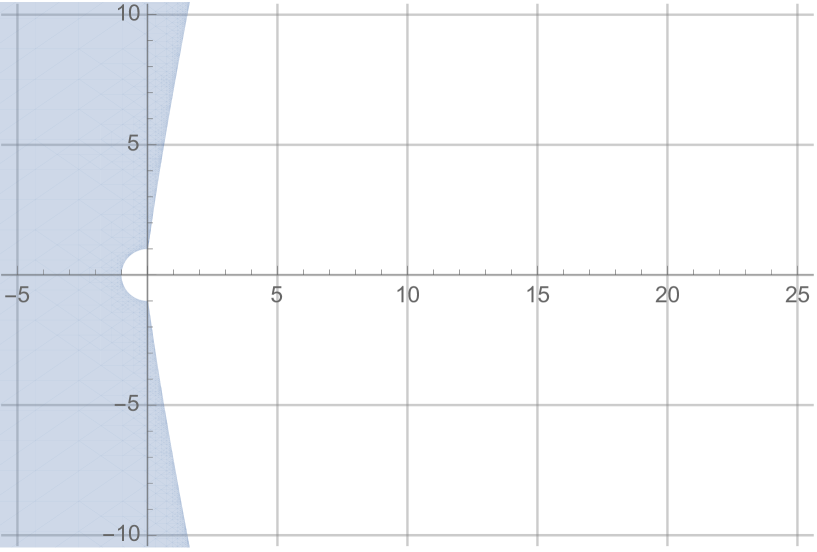
(a) $0<\frac{1}{q}-\min\{0,\frac{d-4}{2d}\}\ll 1$.

(b) $\min\{0,\frac{d-4}{2d}\}<\frac{1}{q}<\frac{d-1}{d}-\frac{1}{2}$.

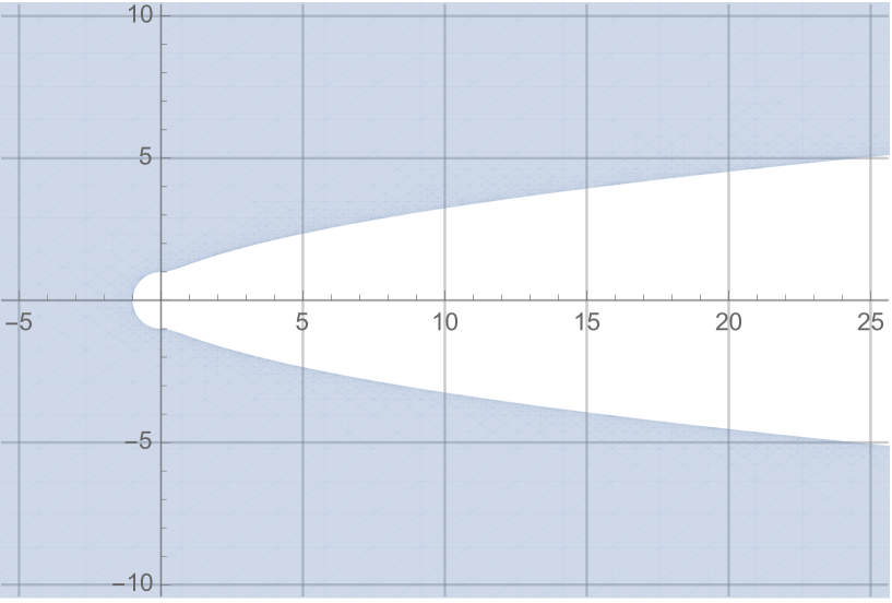
(c) $\min\{0,\frac{d-4}{2d}\}<\frac{1}{q}<\frac{d-1}{d}-\frac{1}{2}$.

(d) $(\frac{1}{p},\frac{1}{q})=(\frac{1}{2},\frac{d-1}{d}-\frac{1}{2})$.

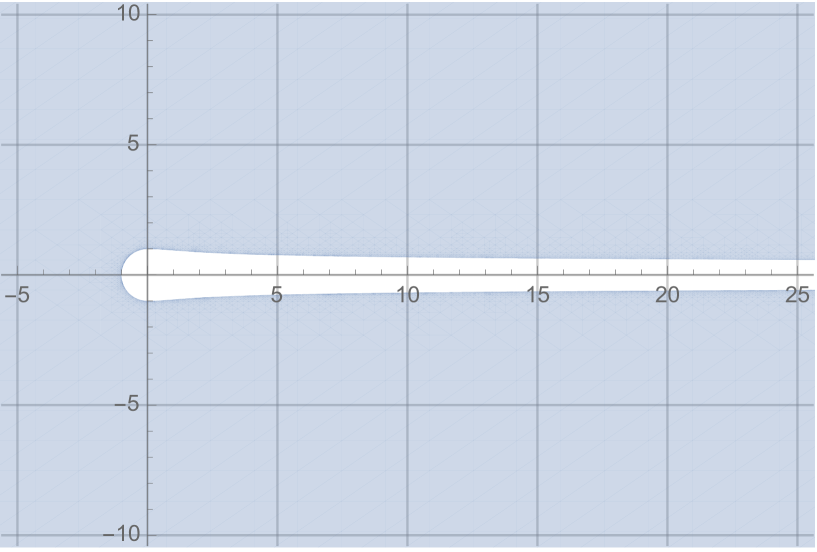
(e) $\frac{d-1}{d}-\frac{1}{2}<\frac{1}{q}<\frac{1}{2}$.

(f) $(\frac{1}{p},\frac{1}{q})=(\frac{1}{2},\frac{1}{2})$.

Figure 9. $\mathcal{Z}_{2,q}(1)$ ((a) $\to$ (b) $\to$ (c) $\to$ (d) $\to$ (e) $\to$ (f)) as $\frac{1}{q}\in\big{(}\min\{0,\frac{d-4}{2d}\},\frac{1}{2}\big{]}$ increases.

The case $\omega_{p,q}=0$

In this case the shape of $\mathcal{Z}_{p,q}(\ell)$ depends on the value of $\ell$ as well.

• Let $(1/p,1/q)\in(A,A^{\prime})$. Since $\omega_{p,q}=\gamma_{p,q}=0$, we have $\mathcal{Z}_{p,q}(\ell)=\emptyset$ if $\ell<1$, and $\mathcal{Z}_{p,q}(\ell)=\mathbb{C}\setminus[0,\infty)$ if $\ell\geq 1$.

• Let $d\geq 4$ and $(\frac{1}{p},\frac{1}{q})\in((\frac{2}{d},0),A)$. In this case $\omega_{p,q}=0$ and $\gamma_{p,q}=\frac{d+1}{2}-\frac{d}{p}\in(0,\frac{d-3}{2})$.

  • If $\ell<1$, $\mathcal{Z}_{p,q}(\ell)=\emptyset$.

  • If $\ell=1$, there is a rigid dichotomy of $\mathcal{Z}_{p,q}(1)$ between the case of uniform bound and the other case; $\mathcal{Z}_{p,q}(1)=\mathbb{C}\setminus[0,\infty)$ if $(1/p,1/q)\in(A,A^{\prime})$, but $\mathcal{Z}_{p,q}(1)=\{z:\mathop{\mathrm{Re}}z\leq 0\}\setminus\{0\}$ if $(1/p,1/q)\notin[A,A^{\prime}]$.

  • When $\ell>1$, there is also a kind of dichotomy although it is not so rigid as in the former case with $\ell=1$. Indeed, if $\ell>1$ and $(1/p,1/q)\in(A,A^{\prime})$, then $\mathcal{Z}_{p,q}(\ell)=\mathbb{C}\setminus[0,\infty)$. Otherwise, $\mathcal{Z}_{p,q}(\ell)$ is the complement (in $\mathbb{C}$) of a (planar) cone of which axis is the positive real line $[0,\infty)$, and apex is the origin. It is interesting to note that, as $(1/p,1/q)$ moves from (near) $A$ to (near) $(2/d,0)$ along the line $1/p-1/q=2/d$, the apex angle gets larger from $0$ to $2\arctan\big{(}1/\sqrt{\ell^{\frac{4}{d-3}}-1}\big{)}$. See Figure 10.

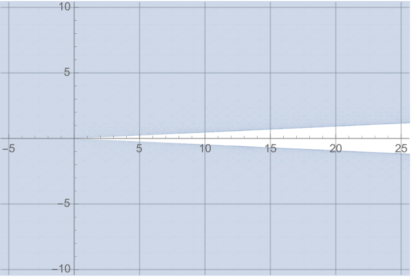
(a) $0<\frac{d+1}{2d}-\frac{1}{p}\ll 1$.

(b) $\frac{2}{d}<\frac{1}{p}<\frac{d+1}{2d}$.

(c) $0<\frac{1}{p}-\frac{2}{d}\ll 1$.

Figure 10. $\mathcal{Z}_{p,q}(\ell)$ with $\ell>1$ ((a) $\to$ (b) $\to$ (c)) as $\frac{1}{p}$ decreases in the interval $(\frac{2}{d},\frac{d+1}{2d})$ along the line $\frac{1}{p}-\frac{1}{q}=\frac{2}{d}$ and $d\geq 4$.

5. Lower bounds for $\|(-\Delta-z)^{-1}\|_{p\to q}$: Proposition 1.3

In this section we obtain lower bounds for $\|(-\Delta-z)^{-1}\|_{p\to q}$, which prove Proposition 1.3. Before doing this we provide proof of Proposition 1.1 which is simpler.

5.1. Proof of Proposition 1.1

We first show the sufficiency part. By (1.4) it is sufficient to show the estimate

(5.1) $$\Big{\|}\mathcal{F}^{-1}\Big{(}\frac{\widehat{f}(\xi)}{|\xi|^{2}-z}\Big{)}\Big{\|}_{q}\leq C_{z}\|f\|_{p}$$

holds whenever $(1/p,1/q)\in\mathcal{R}_{0}$. Since $z\neq 0$, thanks to the scaling property (1.5) we may assume that $z\in\mathbb{S}^{1}\setminus\{1\}$. Let us break the multiplier

$$(|\xi|^{2}-z)^{-1}=\beta_{0}(|\xi|)(|\xi|^{2}-z)^{-1}+\sum_{j\geq 0}\beta(2^{-j}|\xi|)(|\xi|^{2}-z)^{-1}.$$

It is clear that $\beta_{0}(|\xi|)(|\xi|^{2}-z)^{-1}$ is smooth and compactly supported in the open ball $B_{d}(0,3/4)$. Hence

(5.2) $$\Big{\|}\mathcal{F}^{-1}\Big{(}{\beta_{0}(|\xi|)}({|\xi|^{2}-z})^{-1}\widehat{f}(\xi)\Big{)}\Big{\|}_{q}\leq C\|f\|_{p}$$

for $p,q$ satisfying $1\leq p\leq q\leq\infty$. By scaling it is easy to see $\big{\|}\mathcal{F}^{-1}\big{(}\frac{\beta(2^{-j}|\xi|)}{|\xi|^{2}-z}\big{)}\big{\|}_{r}\lesssim 2^{(d-2-\frac{d}{r})j}$ for $1\leq r\leq\infty$. Thus, Young’s inequality gives

$$\Big{\|}\mathcal{F}^{-1}\Big{(}\frac{{\beta(2^{-j}|\xi|)}\widehat{f}(\xi)}{|\xi|^{2}-z}\Big{)}\Big{\|}_{q}\lesssim 2^{j(\frac{d}{p}-\frac{d}{q}-2)}\|f\|_{p}$$

whenever $1\leq p\leq q\leq\infty$. Thus summation along $j$ and combining the resulting estimate with (5.2) give all desired estimates (5.1) except the case $1/p-1/q=2/d$. In order to obtain the estimate (5.1) for $p,q$ with $1/p-1/q=2/d$ in the case $d\geq 3$, we use $(\mathrm{I}\!\mathrm{I}\!\mathrm{I})$ in Lemma 2.15 with $k=1$ to get

$$\Big{\|}\sum_{j\geq 1}\mathcal{F}^{-1}\Big{(}{\beta(2^{-j}|\xi|)}({|\xi|^{2}-z})^{-1}\widehat{f}(\xi)\Big{)}\Big{\|}_{q,\infty}\lesssim\|f\|_{p}$$

provided that $1\leq p,q<\infty$ and $1/p-1/q=2/d$. Real interpolation between those estimates together with (5.2) gives the desired estimate (5.1) for all $p,q$ satisfying $(1/p,1/q)\in\mathcal{R}_{0}$.

Now we consider the necessity part of Proposition 1.1. In the case $d\geq 3$ we need to show (5.1) holds only if

(5.3) $$\frac{1}{p}-\frac{1}{q}\geq 0,\quad\frac{1}{p}-\frac{1}{q}\leq\frac{2}{d},\quad(p,q)\neq\Big{(}1,\,\frac{d}{d-2}\Big{)},\quad(p,q)\neq\Big{(}\frac{d}{2},\,\infty\Big{)}.$$

The first condition is obvious since the multiplier operator is translation invariant ([26]). For the second condition we notice that, for large $j$, the estimate (5.1) remains valid with $C$ independent of $j$ if $\widehat{f}(\xi)$ is replaced with $\beta(2^{-j}|\xi|)\widehat{f}(\xi)$. Then re-scaling the estimate gives

(5.4) $$\Big{\|}\mathcal{F}^{-1}\Big{(}\frac{\beta(|\xi|)\widehat{f}(\xi)}{|\xi|^{2}-2^{-2j}z}\Big{)}\Big{\|}_{q}\leq C_{z}2^{j(2+\frac{d}{q}-\frac{d}{p})}\|f\|_{p}$$

for $f\in\mathcal{S}(\mathbb{R}^{d}).$ Now fix a nonzero Schwartz function $f$ such that $\|\mathcal{F}^{-1}(|\xi|^{-2}\beta(|\xi|)\widehat{f}(\xi))\|_{q}>0$. If we take limit $j\to+\infty$ the left side of (5.4) converges to $\|\mathcal{F}^{-1}(|\xi|^{-2}\beta(|\xi|)\widehat{f}(\xi))\|_{q}$, but the quantity $2^{j(2+d/q-d/p)}$ on the right side converges to zero when $1/p-1/q>2/d$. Therefore any estimate of the form (5.1) is possible only if $1/p-1/q\leq 2/d$. This gives the second condition in (5.3). Finally, to show the last two conditions, by duality we need only show one of them. Suppose (5.1) is true with $(p,q)=(1,d/(d-2))$. Then by (5.1) and (5.2) we see that

$$\Big{\|}\mathcal{F}^{-1}\Big{(}(1-\beta_{0}(|\xi|))(|\xi|^{2}-z)^{-1}\widehat{f}(\xi)\Big{)}\Big{\|}_{\frac{d}{d-2}}\leq C\|f\|_{1}.$$

We now note that $1-\beta_{0}(|\xi|)=(1-\beta_{0}(4|\xi|))(1-\beta_{0}(|\xi|))$. By Mikhlin’s multiplier theorem (applied to the multiplier operator given by $(1-\beta_{0}(4|\xi|))(|\xi|^{2}-z)|\xi|^{-2}$) we see that

$$\Big{\|}\mathcal{F}^{-1}\Big{(}(1-{\beta_{0}(|\xi|)})|\xi|^{-2}\widehat{f}(\xi)\Big{)}\Big{\|}_{\frac{d}{d-2}}\leq C\|f\|_{1}.$$

By scaling this also implies, for all $\epsilon>0$,

$$\Big{\|}\mathcal{F}^{-1}\Big{(}(1-{\beta_{0}(\epsilon|\xi|)})|\xi|^{-2}\widehat{f}(\xi)\Big{)}\Big{\|}_{\frac{d}{d-2}}\leq C\|f\|_{1}.$$

Letting $\epsilon\to 0$ gives $\|\mathcal{F}^{-1}(|\xi|^{-2}\widehat{f}(\xi))\|_{\frac{d}{d-2}}\leq C\|f\|_{1}$ which is obviously not true. Therefore we conclude the estimate (5.1) cannot be true with $p=1$ and $q=d/(d-2)$.

When $d=2$ the above argument works for $p,q$ satisfying $1/p-1/q<2/d$, but not for $p,q$ with $1/p-1/q=2/d$, that is, $p=1$, $q=\infty$ because Mikhlin’s theorem does not hold with $q=\infty$. So we still need to show the failure of (5.1) with $p=1$, $q=\infty$. But the failure can be shown in a more straightforward manner. We need to prove that for any fixed $z\in\mathbb{C}\setminus[0,\infty)$ there does not exist a constant $C>0$ such that

(5.5) $$\|(-\Delta-z)^{-1}f\|_{L^{\infty}(\mathbb{R}^{2})}\leq C\|f\|_{L^{1}(\mathbb{R}^{2})},\quad\forall f\in L^{1}(\mathbb{R}^{2}).$$

To show this let us assume (5.5) and recall from [50, p. 202] that

$$(-\Delta-z)^{-1}f(x)=(2\pi)^{-1}\int_{\mathbb{R}^{2}}K_{0}(\sqrt{-z}\,|x-y|)f(y)dy,$$

where $K_{\nu}(w)$ is the modified Bessel function of the second kind (see [39, 50]). It is well-known ([39, p. 252]) that

(5.6) $$\lim_{w\to 0}\frac{K_{0}(w)}{-\ln w}=1.$$

Let us choose a $\phi\in C^{\infty}_{0}(B_{2}(0,1))$ such that $\phi\geq 0$ and $\|\phi\|_{1}=1$, and set $\phi_{\epsilon}(x)=\epsilon^{-2}\phi(\epsilon^{-1}x)$, $\epsilon>0$. Testing (5.5) with $f=\phi_{\epsilon}$ and letting $\epsilon\to 0$ yield $\sup_{x\in\mathbb{R}^{2}}\big{|}K_{0}(\sqrt{-z}\,|x|)\big{|}\lesssim 1$. This contradicts the asymptotic (5.6), thus we conclude (5.5) fails. ∎

5.2. Proof of Proposition 1.3

For a bounded function $m(\xi)$ which is symmetric under reflection $\xi\to-\xi$ it is easy to see that the $L^{p}$–$L^{q}$ norms of the operators $m(D)$ and $\overline{m}(D)$ are equal, hence we have

$$\|(m\pm\overline{m})(D)\|_{p\to q}\leq 2\|m(D)\|_{p\to q}.$$

Therefore, to prove the lower bounds (1.13), we may work with the imaginary part

$$\mathop{\mathrm{Im}}\Big{(}\frac{1}{|\xi|^{2}-z}\Big{)}=\frac{1}{2i}\Big{(}\frac{1}{|\xi|^{2}-z}-\frac{1}{|\xi|^{2}-\bar{z}}\Big{)}=\frac{\mathop{\mathrm{Im}}z}{(|\xi|^{2}-\mathop{\mathrm{Re}}z)^{2}+(\mathop{\mathrm{Im}}z)^{2}}.$$

The lower bounds in (1.13) is meaningful only when $0<|\mathop{\mathrm{Im}}z|\ll\mathop{\mathrm{Re}}z<1$. Hence we only need to consider $z=1+i\delta$ with $0<100\delta<1$ in this section. The lower bound $\gtrsim 1$ (in the case of $\gamma_{p,q}=0$) is clear since the resolvent operators are nontrivial. Thus, recalling (1.8) it is sufficient to show that

$$\Big{\|}\mathcal{F}^{-1}\Big{(}\frac{\delta\widehat{f}(\xi)}{(|\xi|^{2}-1)^{2}+\delta^{2}}\Big{)}\Big{\|}_{q}\gtrsim\max\big{\{}\delta^{-1+\frac{d+1}{2}(\frac{1}{p}-\frac{1}{q})},\delta^{\frac{d-1}{2}-\frac{d}{q}}\big{\}}\|f\|_{p}.$$

for $f\in L^{p}(\mathbb{R}^{d})$. The other lower bound $\delta^{\frac{d}{p}-\frac{d+1}{2}}$ in (1.13) follows from the lower bound $\delta^{\frac{d-1}{2}-\frac{d}{q}}$ by duality. Since we also consider the resolvent estimates for the fractional Laplacian in Section 6 we prove this in a slightly more general form. The argument is based on the counterexamples related to the restriction conjecture: a Knapp type example and the Fourier transform of the surface measure on the sphere (see [46, pp. 387–388]).

Lemma 5.1.

Let $1\leq p,q\leq\infty$, and for $r,s>0$ let $m_{\delta}^{s}(r):=\frac{\delta}{(r^{s}-1)^{2}+\delta^{2}}$. Then, if $0<\delta<c$ for a small $c>0$,

(5.7) $$\|m_{\delta}^{s}(|D|)\|_{p\to q} \gtrsim\delta^{-1+\frac{d+1}{2}(\frac{1}{p}-\frac{1}{q})},$$

(5.8) $$\|m_{\delta}^{s}(|D|)\|_{p\to q} \gtrsim\delta^{\frac{d-1}{2}-\frac{d}{q}},$$

where the implicit constants depend only on $p$, $q$, $s$ and $d$.

Proof of (5.7).

Let $c,k$ be positive constants to be chosen later, depending only on $d$ and $s$. If $|\xi_{j}|\leq c\sqrt{\delta}$, $j=1,\dots,d-1$ and $k\delta/4\leq\xi_{d}-1\leq k\delta$, then

$$0<|\xi|^{s}-1\leq\left(1+\left((d-1)c^{2}+2k+10^{-2}{k^{2}}\right)\delta\right)^{s/2}-1$$

provided that $0<100\delta\leq 1$. Let us set $\mu(t):=(1+t)^{s/2}$ and $M_{s}:=\max\{|\mu^{\prime\prime}(t)|:0\leq t\leq 1\}$. Then, from Taylor’s theorem it follows that

$$0<|\xi|^{s}-1\leq s\left((d-1)c^{2}+2k+10^{-2}{k^{2}}\right)\delta$$

if we choose $\delta$ small enough, that is to say, $0<\big{(}(d-1)c^{2}+2k+10^{-2}{k^{2}}\big{)}\delta\leq\min\big{\{}1,s/M_{s}\big{\}}$. We now choose $c=1/\sqrt{2(d-1)s}$ and $k$ as the positive solution of the quadratic equation $2k+10^{-2}k^{2}=1/2s$ so that, for $0<\delta\leq\min\big{\{}s,s^{2}/M_{s}\big{\}}$,

$$0<|\xi|^{s}-1\leq\delta.$$

Let us set $c_{s}:=\min\big{\{}10^{-2},s,s^{2}/M_{s}\big{\}}$, and choose $\phi,\,\psi\in C^{\infty}_{0}(\mathbb{R})$ such that $\operatorname{supp}\phi\subset[-1,1]$, $0\leq\phi\leq 1$, $\phi=1$ on $[-1/2,1/2]$, $\operatorname{supp}\psi\subset[1/4,1]$, $0\leq\psi\leq 1$ and $\psi=1$ on $[1/2,3/4]$. For every $\delta\in(0,c_{s})$ we define $f_{\delta}\in\mathcal{S}(\mathbb{R}^{d})$ by

$$\widehat{f_{\delta}}(\xi)=\psi\Big{(}\frac{\xi_{d}-1}{k\delta}\Big{)}\prod_{j=1}^{d-1}\phi\Big{(}\frac{\xi_{j}}{c\sqrt{\delta}}\Big{)}.$$

Since $|\int m_{\delta}^{s}(|\xi|)\widehat{f_{\delta}}(\xi)e^{ix\cdot\xi}d\xi|=|\int m_{\delta}^{s}(|\xi|)\widehat{f_{\delta}}(\xi)e^{i(x\cdot\xi-x_{d})}d\xi|$, we have

$$\Big{|}\int m_{\delta}^{s}(|\xi|)\widehat{f_{\delta}}(\xi)e^{ix\cdot\xi}d\xi\Big{|}\geq\Big{|}\int m_{\delta}^{s}(|\xi|)\widehat{f_{\delta}}(\xi)\cos(x\cdot\xi-x_{d})d\xi\Big{|}-\Big{|}\int m_{\delta}^{s}(|\xi|)\widehat{f_{\delta}}(\xi)\sin(x\cdot\xi-x_{d})d\xi\Big{|}.$$

On $\operatorname{supp}\widehat{f_{\delta}}$, $|\xi_{j}|\leq c\sqrt{\delta}$ for $j=1,\cdots,d-1$ and $k\delta/4\leq\xi_{d}-1\leq k\delta$. Thus $m_{\delta}^{s}(|\xi|)\geq 1/2\delta$ whenever $\xi\in\operatorname{supp}\widehat{f_{\delta}}$ and $0<\delta<c_{s}$. Also, if $\xi\in\operatorname{supp}\widehat{f_{\delta}}$ and

$$x\in\mathcal{A}_{\delta}:=\Big{\{}x\in\mathbb{R}^{d}:|x_{j}|\leq\frac{1}{200(d-1)c\sqrt{\delta}},\,j=1,\cdots,d-1,\,|x_{d}|\leq\frac{1}{200k\delta}\Big{\}},$$

then $|x\cdot\xi-x_{d}|\leq 1/100$, hence

$$\Big{|}\int_{\mathbb{R}^{d}}m_{\delta}^{s}(|\xi|)\widehat{f_{\delta}}(\xi)e^{ix\cdot\xi}d\xi\Big{|}\geq\frac{1}{2\delta}\int\widehat{f_{\delta}}(\xi)\Big{(}1-\frac{1}{100}\Big{)}d\xi-\frac{1}{100\delta}\int\widehat{f_{\delta}}(\xi)d\xi\approx\delta^{-1}\|\widehat{f_{\delta}}\|_{1}\approx\delta^{\frac{d-1}{2}}.$$

Integration on the box $\mathcal{A}_{\delta}$ yields

$$\Big{\|}\int_{\mathbb{R}^{d}}m_{\delta}^{s}(|\xi|)\widehat{f_{\delta}}(\xi)e^{ix\cdot\xi}d\xi\Big{\|}_{q}\gtrsim\delta^{\frac{d-1}{2}}|\mathcal{A}_{\delta}|^{1/q}\approx\delta^{\frac{d-1}{2}-\frac{d+1}{2q}}.$$

On the other hand it is easy to check that $\|f_{\delta}\|_{p}\approx\delta^{\frac{d+1}{2}-\frac{d+1}{2p}}$. Thus we obtain (5.7). ∎

Proof of (5.8).

Let $\phi$ be a non-negative smooth function on $\mathbb{R}$ such that $\operatorname{supp}\phi\subset(1-2\varepsilon_{\circ},1+2\varepsilon_{\circ})$ for some small $\varepsilon_{\circ}>0$ to be determined later depending on $s$. We take $f\in C^{\infty}_{0}(\mathbb{R}^{d})$ so that $\widehat{f}(\xi)=\phi(|\xi|)$ and set

$$Q(x):=\int_{\mathbb{R}^{d}}m_{\delta}^{s}(|\xi|)\widehat{f}(\xi)e^{ix\cdot\xi}d\xi.$$

By the spherical coordinate we write

$$Q(x)=(2\pi)^{\frac{d}{2}}\int_{1-2\varepsilon_{\circ}}^{1+2\varepsilon_{\circ}}m_{\delta}^{s}(r)\,\phi(r)r^{d-1}|rx|^{\frac{2-d}{2}}J_{\frac{d-2}{2}}(|rx|)dr,$$

where $J_{\nu}$ denotes the Bessel function of order $\nu$. It is well-known (see [46, p. 338]) that for $\nu>-1/2$

(5.9) $$J_{\nu}(r)=\left(\frac{\pi r}{2}\right)^{-\frac{1}{2}}\cos\left(r-\frac{\pi\nu}{2}-\frac{\pi}{4}\right)+R_{\nu}(r),\quad r>0,$$

where $R_{\nu}$ satisfies $|R_{\nu}(r)|\leq c_{\nu}r^{-3/2}$ if $r\geq 1$.

By (5.9) with $\nu=\frac{d-2}{2}$ and the formula $\cos(u+v)=\cos u\cos v-\sin u\sin v$, we write $Q$ as follows:

$$Q(x)=Q_{1}(x)-Q_{2}(x)+Q_{3}(x),$$

where

(5.10) $$Q_{1}(x) :=2(2\pi)^{\frac{d-1}{2}}|x|^{\frac{1-d}{2}}\cos\Big{(}|x|-\frac{\pi(d-1)}{4}\Big{)}\int_{1-2\varepsilon_{\circ}}^{1+2\varepsilon_{\circ}}m_{\delta}^{s}(r)\,\phi(r)r^{\frac{d-1}{2}}\cos\left((r-1)|x|\right)dr,$$

$$Q_{2}(x) :=2(2\pi)^{\frac{d-1}{2}}|x|^{\frac{1-d}{2}}\sin\Big{(}|x|-\frac{\pi(d-1)}{4}\Big{)}\int_{1-2\varepsilon_{\circ}}^{1+2\varepsilon_{\circ}}m_{\delta}^{s}(r)\,\phi(r)r^{\frac{d-1}{2}}\sin\left((r-1)|x|\right)dr,$$

$$Q_{3}(x) :=(2\pi)^{\frac{d}{2}}\int_{1-2\varepsilon_{\circ}}^{1+2\varepsilon_{\circ}}m_{\delta}^{s}(r)\,\phi(r)r^{d-1}|rx|^{\frac{2-d}{2}}R_{\frac{d-2}{2}}(|rx|)dr.$$

We now split the domain of the integral $\int_{1-2\varepsilon_{\circ}}^{1+2\varepsilon_{\circ}}m_{\delta}^{s}(r)\phi(r)r^{\frac{d-1}{2}}\cos((r-1)|x|)dr$ of $Q_{1}(x)$ into subintervals on which $|r-1|\lesssim\delta$ and $|r-1|\gtrsim\delta$, respectively. To be precise let us set $k(t):=\int_{|\tau|\leq t}\frac{1}{\tau^{2}+1}d\tau$ and fix a large $\lambda>0$ such that

(5.11) $$k(s\lambda)\geq 100(\pi-k(s\lambda)).$$

Clearly, such $\lambda$ exists since $\int_{-\infty}^{\infty}\frac{1}{\tau^{2}+1}d\tau=\pi$. Let $\mu$ be a small number so that $\lambda\mu\leq 10^{-2}$, and let

$$\mathcal{A}^{\prime}:=\Big{\{}x\in\mathbb{R}^{d}:\frac{\mu}{4\delta}\leq|x|\leq\frac{\mu}{2\delta}\Big{\}}.$$

Put $\psi(r):=r^{s}-1$, $r>0$ and set $M_{s}:=\max\{|\psi^{\prime\prime}(r)|:|r-1|\leq 1/2\}$. By Taylor’s theorem, $|\psi(r)-s(r-1)|\leq{M_{s}}(r-1)^{2}/2$ when $|r-1|\leq 1/2$. Thus, if $|\psi(r)|\leq s\lambda\delta$, then

$$|r-1|\leq\frac{M_{s}}{2s}(r-1)^{2}+\frac{|\psi(r)|}{s}\leq\frac{M_{s}\varepsilon_{\circ}}{s}|r-1|+\lambda\delta,\quad\forall r\in\operatorname{supp}\phi\cap[1/2,3/2].$$

Choosing $\varepsilon_{\circ}:=\min\{s/(2M_{s}),1/4\}$ we have $|r-1|\leq 2\lambda\delta$ on $\operatorname{supp}\phi$ whenever $|\psi(r)|\leq s\lambda\delta$. Therefore, if $x\in\mathcal{A}^{\prime}$ and $|\psi(r)|\leq s\lambda\delta$, then $|(r-1)x|\leq\lambda\mu\leq 10^{-2}$, so $\cos((r-1)|x|)\geq 99/100$ on $\operatorname{supp}\phi$.

Now we break the integral part of $Q_{1}(x)$ as the following:

$$I_{1}(x)+I_{2}(x):=\Big{(}\int_{|\psi(r)|\leq s\lambda\delta}+\int_{|\psi(r)|>s\lambda\delta}\Big{)}\frac{\delta}{\psi(r)^{2}+\delta^{2}}\,\phi(r)r^{\frac{d-1}{2}}\cos\left((r-1)|x|\right)dr.$$

If $x\in\mathcal{A}^{\prime}$, by the above choice of $\lambda$ and $\varepsilon_{\circ}$, we have

$$I_{1}(x)\geq\frac{99}{100}\int_{|\psi(r)|\leq s\lambda\delta}\frac{\delta}{\psi(r)^{2}+\delta^{2}}\,\phi(r)r^{\frac{d-1}{2}-s+1}\frac{d\psi(r)}{s}.$$

Hence, we choose $\phi\in C_{0}^{\infty}((1-2\varepsilon_{\circ},1+2\varepsilon_{\circ}))$ such that $\phi(r)r^{\frac{d-1}{2}-s+1}=1$ if $|r-1|\leq\varepsilon_{\circ}$, and $0\leq\phi(r)r^{\frac{d-1}{2}-s+1}\leq 2$ for all $r$. Thus it follows that, if $x\in\mathcal{A}^{\prime}$ and $\delta\leq\varepsilon_{\circ}/(2\lambda)$, then

$$I_{1}(x)\geq\frac{99}{100s}\int_{|t|\leq s\lambda\delta}\frac{\delta}{t^{2}+\delta^{2}}dt=\frac{99}{100s}k(s\lambda).$$

On the other hand, by our choice of $\phi$ and (5.11)

$$|I_{2}(x)|\leq\int_{|\psi(r)|>s\lambda\delta}\frac{\delta}{\psi(r)^{2}+\delta^{2}}\,\phi(r)r^{\frac{d-1}{2}-s+1}\frac{d\psi(r)}{s}\leq\frac{2}{s}\big{(}\pi-k(s\lambda)\big{)}\leq\frac{k(s\lambda)}{50s}.$$

Therefore we have, for $x\in\mathcal{A}^{\prime}$ and $0<\delta\leq\varepsilon_{\circ}/(2\lambda)$,

(5.12) $$I_{1}(x)+I_{2}(x)\geq I_{1}(x)-|I_{2}(x)|\geq\frac{97k(s\lambda)}{100s}.$$

For each $n\in\mathbb{N}$ let us set

$$\mathcal{A}_{n}:=\Big{\{}x\in\mathcal{A}^{\prime}:\pi\Big{(}2n+\frac{d-1}{4}\Big{)}-\frac{1}{100}\leq|x|\leq\pi\Big{(}2n+\frac{d-1}{4}\Big{)}+\frac{1}{100}\Big{\}},$$

which is nonempty only if $n\approx\delta^{-1}$. We also set

$$\mathcal{A}:=\bigcup_{n\in\mathbb{N}}A_{n}.$$

From now on suppose that $x\in\mathcal{A}$. It is clear that $\cos(|x|-\pi(d-1)/4)\geq 99/100$, and $|\sin(|x|-\pi(d-1)/4)|\leq 1/100$. Hence, when $0<\delta\leq\varepsilon_{\circ}/(2\lambda)$ it follows from (5.10) and (5.12) that

$$Q_{1}(x)\geq 2(2\pi)^{\frac{d-1}{2}}|x|^{\frac{1-d}{2}}\cdot\frac{99}{100}\cdot\frac{97k(s\lambda)}{100s}.$$

Similarly, we get

$$|Q_{2}(x)|\leq 2(2\pi)^{\frac{d-1}{2}}|x|^{\frac{1-d}{2}}\cdot\frac{2}{100s}\cdot\frac{101\,k(s\lambda)}{100}.$$

Combining the estimates for $Q_{1}(x)$ and $|Q_{2}(x)|$, we have

$$Q_{1}(x)-Q_{2}(x)\gtrsim|x|^{\frac{1-d}{2}}\approx\delta^{\frac{d-1}{2}},$$

where the implicit constants depend only on $d$ and $s$. On the other hand, it is straightforward to see that $Q_{3}(x)=O(\delta^{\frac{d+1}{2}})$ as $\delta\to 0$. Thus, with sufficiently small $\delta$, we have that

$$Q(x)=Q_{1}(x)-Q_{2}(x)+Q_{3}(x)\gtrsim\delta^{\frac{d-1}{2}},\quad\forall x\in\mathcal{A}.$$

Observe that we can choose a constant $c\in(0,1/10)$, independent of all small $\delta>0$, such that $|\mathcal{A}|\geq c|B(0,\mu(2\delta)^{-1})|$. Therefore, we conclude that

$$\left\|Q\right\|_{L^{q}(\mathcal{A})}\gtrsim\delta^{\frac{d-1}{2}-\frac{d}{q}}$$

for all sufficiently small $\delta>0$, with the implicit constant depending only on $d,s$. Meanwhile, $f=\mathcal{F}^{-1}(\phi(|\cdot|))\in L^{p}(\mathbb{R}^{d})$ for any $p\in[1,\infty]$. Thus, this completes the proof of (5.8). ∎

6. Sharp resolvent estimates for the fractional Laplace operators

The resolvent estimates for $(-\Delta)^{\frac{s}{2}}$ can be obtained by making use of the argument we have used for the resolvent estimates for $-\Delta$ (the case $s=2$). In technical aspect there is not much difference, but it is worthwhile to record the result for the operator $((-\Delta)^{\frac{s}{2}}-z)^{-1}$. We shall be brief, but include the statements of results and sketch their proofs. In what follows we consider $s\in(0,d)$ though generalization to $s\geq d$ is also possible.

We begin with the following which can be shown by adapting the proof of Proposition 1.1, so we state it without proof.

Proposition 6.1.

Let $d\geq 2$, $0<s<d$, $1\leq p,q\leq\infty$ and let $z\in\mathbb{C}\setminus[0,\infty)$. Then, $\|((-\Delta)^{\frac{s}{2}}-z)^{-1}\|_{p\to q}<\infty$ if and only if $(1/p,1/q)\in\mathcal{R}^{s}_{0}$ which is given by

$$\mathcal{R}^{s}_{0}=\mathcal{R}^{s}_{0}(d):=\Big{\{}(x,y)\in I^{2}:0\leq x,y\leq 1,~{}0\leq x-y\leq\frac{s}{d}\Big{\}}\setminus\Big{\{}\Big{(}1,\frac{d-s}{d}\Big{)},\Big{(}\frac{s}{d},0\Big{)}\Big{\}}.$$

We introduce some notations which we need to state our results. For $d\geq 2$ and $0<s<d$, let us define $\mathcal{R}^{s}_{1}=\mathcal{R}^{s}_{1}(d),$ $\mathcal{R}^{s}_{2}=\mathcal{R}^{s}_{2}(d)$, and $\mathcal{R}^{s}_{3}=\mathcal{R}^{s}_{3}(d)$ by

$$\mathcal{R}^{s}_{1}:=\mathcal{P}(d)\cap\mathcal{R}^{s}_{0}(d),\quad\mathcal{R}^{s}_{2}:=\big{(}\mathcal{T}(d)\cap\mathcal{R}^{s}_{0}(d)\big{)}\setminus\big{(}[D,H)\cup[D^{\prime},H)\big{)},\quad\mathcal{R}^{s}_{3}:=\mathcal{Q}(d)\cap\mathcal{R}^{s}_{0}(d).$$

Note that if $0<s<\frac{2d}{d+1}$, $\mathcal{R}^{s}_{1}=\emptyset$ (see Figure 12), and $\mathcal{R}^{2}_{i}=\mathcal{R}_{i}$ for $i=0,1,2,3$. If $0<s<2$, then $\mathcal{R}^{s}_{i}=\mathcal{R}_{i}\cap\mathcal{R}^{s}_{0}$ for every $i$. From the definition of $\gamma_{p,q}$ (recall (1.8)), it follows that (1.12) holds with $\mathcal{R}_{i}$ replaced by ${\mathcal{R}}^{s}_{i}$, $i=1,2,3$.

Figure 11. The case $d\geq 3$, $0<s<\frac{2d}{d+1}$

Figure 12. The case $d\geq 3$, $\frac{2d}{d+1}\leq s<d$

As before, by scaling we have $\|((-\Delta)^{\frac{s}{2}}-z)^{-1}\|_{p\to q}=|z|^{-1+\frac{d}{s}(\frac{1}{p}-\frac{1}{q})}\|((-\Delta)^{\frac{s}{2}}-|z|^{-1}z)^{-1}\|_{p\to q}$ for $z\in\mathbb{C}\setminus[0,\infty)$. Using Lemma 5.1 we may repeat the argument in the proof of Proposition 1.3 to get

$$\|((-\Delta)^{\frac{s}{2}}-z)^{-1}\|_{p\to q}\gtrsim\operatorname{dist}(z,[0,\infty))^{-\gamma_{p,q}},\quad z\in\mathbb{S}^{1}\setminus\{1\}.$$

Combining these two, we get, for $z\in\mathbb{C}\setminus[0,\infty)$,

(6.1) $$\|((-\Delta)^{\frac{s}{2}}-z)^{-1}\|_{p\to q}\gtrsim{\kappa}_{p,q}^{s}(z):=|z|^{-1+\frac{d}{s}(\frac{1}{p}-\frac{1}{q})+\gamma_{p,q}}\operatorname{dist}(z,[0,\infty))^{-\gamma_{p,q}},$$

and we may conjecture the following which is a natural extension of Conjecture 1.

Conjecture 3.

Let $d\geq 2$, $0<s<d$ and let $(1/p,1/q)\in\big{(}\bigcup_{i=1}^{3}\mathcal{R}_{i}^{s}\big{)}\cup\mathcal{R}_{3}^{s\prime}$. There exists an absolute constant $C$, depending only on $p$, $q$, $d$ and $s$, such that, for $z\in\mathbb{C}\setminus[0,\infty)$,

(6.2) $$C^{-1}{\kappa}_{p,q}^{s}(z)\leq\|((-\Delta)^{\frac{s}{2}}-z)^{-1}\|_{p\to q}\leq C{\kappa}_{p,q}^{s}(z).$$

When $d\geq 3$ let us set $\widetilde{\mathcal{R}}^{s}_{2}:=\mathcal{R}_{0}^{s}(d)\cap\widetilde{\mathcal{R}}_{2}(d)$ and $\widetilde{\mathcal{R}}^{s}_{3}:={\mathcal{R}}^{s}_{3}(d)\setminus[D,P_{\circ},P_{\ast}]$. We have the following.

Theorem 6.2.

Let $z\in\mathbb{C}\setminus[0,\infty)$. If $d=2$, Conjecture 3 is true. If $d\geq 3$, the conjectured estimate (6.2) is true whenever $(1/p,1/q)\in\mathcal{R}^{s}_{1}\cup\big{(}\bigcup_{i=2}^{3}\widetilde{\mathcal{R}}^{s}_{i}\big{)}\cup\widetilde{\mathcal{R}}^{s\prime}_{3}$. Furthermore, if $d\geq 2$, for $p,q,s$ satisfying $(1/p,1/q)\in\{B,B^{\prime}\}$ and $\frac{2d}{d+1}\leq s<d$ (see Figure 12), we have $\|((-\Delta)^{\frac{s}{2}}-z)^{-1}f\|_{q,\infty}\lesssim|z|^{-1+\frac{2d}{s(d+1)}}\|f\|_{p,1}$ and, for $p,s$ satisfying $(\frac{1}{p},\frac{d-1}{2d})\in(B^{\prime},E^{\prime}]\cap\mathcal{R}^{s}_{0}$ and $\frac{2d}{d+1}<s<d$, we have $\|((-\Delta)^{\frac{s}{2}}-z)^{-1}f\|_{\frac{2d}{d-1},\infty}\lesssim|z|^{-1+\frac{d}{s}(\frac{1}{p}-\frac{1}{q})}\|f\|_{p}.$

We remark that Theorem 1.4 is a special case of Theorem 6.2 when $d\geq 3$. If $\frac{2d}{d+1}\leq s<d$ and $(1/p,1/q)\in\mathcal{R}^{s}_{1}(d)$, Theorem 6.2 covers the result by Huang, Yao and Zheng [29, Theorem 1.4].

Proof of Theorem 6.2.

We basically follow the argument in Section 4 with some modifications. For $z\in\mathbb{S}^{1}\setminus\{1\}$ let us set

$$m^{s}(\xi,z)=(|\xi|^{s}-z)^{-1}.$$

Using the same functions $\rho_{0},$ $\rho_{1},$ and $\rho_{2}$ as in Section 4 we break $m^{s}$ such that $m_{j}^{s}(\xi,z):=m(\xi,z)\rho_{j}(\xi),$ $j=0,1,2,$ and $m^{s}(\xi,z)=\sum_{j=0}^{2}m_{j}^{s}(\xi,z).$ Since $|\partial^{\alpha}_{\xi}m_{2}^{s}(\xi,z)|\lesssim|\xi|^{-s-|\alpha|}$ and $m_{2}^{s}$ is supported away from the orign, by the standard argument (for example, the proof of sufficiency part of Proposition 1.1) we see that $\|m_{2}^{s}(D,z)f\|_{q}\leq C\|f\|_{p}$ if $(1/p,1/q)\in\mathcal{R}^{s}_{0}$. Similarly, since $m_{1}^{s}$ is supported in $B_{d}(0,1)$ and $|\partial^{\alpha}_{\xi}m_{1}^{s}(\xi,z)|\lesssim|\xi|^{s-|\alpha|}$, we see that $\|m_{1}^{s}(D,z)f\|_{q}\leq C\|f\|_{p}$ if $1\leq p\leq q\leq\infty$. Thus, we need only handle $m_{0}^{s}(D,z)$. If $z\in\mathbb{S}^{1}(\theta_{\circ})$, $\partial^{\alpha}_{\xi}m_{0}^{s}({\xi},z)$ is uniformly bounded. So, we may assume $z\not\in\mathbb{S}^{1}(\theta_{\circ})$ and we are reduced to showing (4.5) when $(1/p,1/q)\in\mathcal{R}^{s}_{1}\cup\big{(}\bigcup_{i=2}^{3}\widetilde{\mathcal{R}}^{s}_{i}\big{)}\cup\widetilde{\mathcal{R}}^{s\prime}_{3}$, and its (resticted) weak type variants when $(1/p,1/q)\in[B^{\prime},E^{\prime}]\cap\mathcal{R}_{0}^{s}$. All of these estimates are contained in Proposition 4.1. ∎

6.1. Region of spectral parameters for uniform estimate

Let $p$, $q$, $d$ and $s$ be as in Theorem 6.2, and let $\ell>0$. Making use of Theorem 6.2 we can also describe the region

$$\mathcal{Z}_{p,q}^{s}(\ell):=\big{\{}z\in\mathbb{C}\setminus[0,\infty):{\kappa}_{p,q}^{s}(z)\leq\ell\big{\}}.$$

We consider three cases $0<s<\frac{2d}{d+1}$, $s=\frac{2d}{d+1}$, and $\frac{2d}{d+1}<s<d$, separately. Also, by duality it is sufficient to consider $p,q$ satisfying $(1/p,1/q)\in\mathcal{R}^{s}_{1}\cup\widetilde{\mathcal{R}}^{s}_{2}\cup\widetilde{\mathcal{R}}^{s}_{3}$. As before we set the homogeneity degree $\omega_{p,q}^{s}=\omega_{p,q}^{s}(d):=1-\frac{d}{s}(\frac{1}{p}-\frac{1}{q}),$ which is in $[0,1]$ when $(1/p,1/q)\in\mathcal{R}_{0}^{s}$, and note that

$$\mathcal{Z}_{p,q}^{s}(\ell) =\big{\{}z\in\mathbb{C}\setminus\{0\}:\mathop{\mathrm{Re}}z\leq 0,\,\ell|z|^{\omega_{p,q}^{s}}\geq 1\big{\}}$$

$$\qquad\cup\big{\{}z\in\mathbb{C}\setminus[0,\infty):\mathop{\mathrm{Re}}z>0,\,\ell|\mathop{\mathrm{Im}}z|^{\gamma_{p,q}}\geq|z|^{\gamma_{p,q}-\omega_{p,q}^{s}}\big{\}}.$$

Since $\omega_{2,2}^{s}=1=\gamma_{2,2}$ for any $s$ and $d$, $\mathcal{Z}_{2,2}^{s}(\ell)$ is always the complement of the $\ell^{-1}$-neighborhood of $[0,\infty)$ (see Figure 6(c) or Figure 8(f)). We also note that $\mathcal{Z}_{p,q}^{s}(\ell)=\emptyset$ if $\omega_{p,q}^{s}=0$ and $\ell<1$. In what follows we disregard the case $p=q=2$, and the case $\ell<1$ whenever $\omega_{p,q}^{s}=0$.

When $0<s<\frac{2d}{d+1}$. In this case, $\mathcal{R}_{1}^{s}=\emptyset$, and $\gamma_{p,q}>0$ for all $p,q$ with $(1/p,1/q)\in\widetilde{\mathcal{R}}^{s}_{2}\cup\widetilde{\mathcal{R}}^{s}_{3}$. If $\omega_{p,q}^{s}=0$, $\mathcal{Z}_{p,q}^{s}(1)=\{z\in\mathbb{C}\setminus\{0\}:\mathop{\mathrm{Re}}z\leq 0\}$, and $\mathcal{Z}_{p,q}^{s}(\ell)$ with $\ell>1$ is a complement of a planar cone such as in Figure 10. If $\omega_{p,q}^{s}>0$, one can easily check that $\gamma_{p,q}-\omega_{p,q}^{s}>0$ for all $(1/p,1/q)\in\big{(}\widetilde{\mathcal{R}}_{2}^{s}\setminus\{H\}\big{)}\cup\widetilde{\mathcal{R}}_{3}^{s}$. Thus, $\mathcal{Z}_{p,q}^{s}(\ell)$ has profiles such as the regions in Figure 9(a), Figure 9(b), or Figure 9(c).

When $s=\frac{2d}{d+1}$. In this case, $\frac{1}{p}-\frac{1}{q}=\frac{s}{d}=\frac{2}{d+1}$ and $\mathcal{R}_{1}^{s}=(B,B^{\prime})$. If $\omega_{p,q}^{s}=0$, $\mathcal{Z}_{p,q}^{s}(\ell)=\mathbb{C}\setminus[0,\infty)$ for $(1/p,1/q)\in\mathcal{R}_{1}^{s}$ and $\ell\geq 1$; $\mathcal{Z}_{p,q}^{s}(1)$ is the left half-plane for $(1/p,1/q)\in\widetilde{\mathcal{R}}_{3}^{s}$; $\mathcal{Z}_{p,q}^{s}(\ell)$ is a complement of a planar cone for $(1/p,1/q)\in\mathcal{R}_{3}^{s}$ and $\ell>1$ (see Figure 10); there is no $p,q$ satisfying $(1/p,1/q)\in\mathcal{R}_{2}^{s}$. If $\omega_{p,q}^{s}>0$, we consider the following two cases:

• $(1/p,1/q)\in\widetilde{\mathcal{R}}_{2}^{s}\setminus\{H\}$: In this case, $\gamma_{p,q}-\omega_{p,q}^{s}=0$ since $s=\frac{2d}{d+1}$. Hence, $\mathcal{Z}_{p,q}^{s}(\ell)$ is the complement of the $\ell^{-1/\gamma_{p,q}}$-neighborhood of $[0,\infty)$.

• $(1/p,1/q)\in\widetilde{\mathcal{R}}_{3}^{s}$: Then, $\gamma_{p,q}-\omega_{p,q}^{s}=-\frac{d+1}{2}\big{(}\frac{1}{q}-\frac{d-1}{d+1}(1-\frac{1}{p})\big{)}>0$. Thus, the profiles of $\mathcal{Z}_{p,q}^{s}(\ell)$ take the forms of the regions in Figure 9(a), Figure 9(b), or Figure 9(c).

When $\frac{2d}{d+1}<s<d$. The classification of the profiles of $\mathcal{Z}_{p,q}^{s}(\ell)$ is similar to that in Section 4.4 where $s=2$. Again we consider the cases $\omega_{p,q}^{s}=0$ and $\omega_{p,q}^{s}>0$, separately. If $\omega_{p,q}^{s}=0$, there are only two cases $(1/p,1/q)\in\mathcal{R}_{1}^{s}$ and $(1/p,1/q)\in\widetilde{\mathcal{R}}_{3}^{s}$. For the first case $\mathcal{Z}_{p,q}^{s}(\ell)=\mathbb{C}\setminus[0,\infty)$ when $\ell\geq 1$, and for the latter $\mathcal{Z}_{p,q}^{s}(1)$ is the left half-plane and $\mathcal{Z}_{p,q}^{s}(\ell)$ with $\ell>1$ is the complement of a planar cone (Figure 10). If $\omega_{p,q}^{s}>0$, we consider the following cases:

• $(1/p,1/q)\in\mathcal{R}_{1}^{s}$: Since $\gamma_{p,q}=0$ and $0<\omega_{p,q}^{s}<\frac{s(d+1)-2d}{s(d+1)}$, $\mathcal{Z}_{p,q}^{s}(\ell)=\{z\in\mathbb{C}\setminus[0,\infty):|z|\geq\ell^{-1/\omega_{p,q}}\}$.

• $(1/p,1/q)\in\widetilde{\mathcal{R}}_{2}^{s}\setminus\{H\}$: Since $\gamma_{p,q}-\omega_{p,q}^{s}=(\frac{d}{s}-\frac{d+1}{2})(\frac{1}{p}-\frac{1}{q})<0$, $\mathcal{Z}_{p,q}^{s}(\ell)$ is the complement of a neighborhood of $[0,\infty)$ which shrinks along the positive real line as $\mathop{\mathrm{Re}}z\to\infty$.

• $(1/p,1/q)\in\widetilde{\mathcal{R}}_{3}^{s}$: Note that $\gamma_{p,q}=\frac{d+1}{2}-\frac{d}{p}>0$, and $\gamma_{p,q}-\omega_{p,q}^{s}=\frac{d}{s}(\frac{1-s}{p}+\frac{s(d-1)}{2d}-\frac{1}{q})$. We divide $\widetilde{\mathcal{R}}_{3}^{s}$ into $\widetilde{\mathcal{R}}_{3,+}^{s}$, $\widetilde{\mathcal{R}}_{3,0}^{s}$, and $\widetilde{\mathcal{R}}_{3,-}^{s}$ which are given by

  $$\widetilde{\mathcal{R}}_{3,\pm}^{s} =\Big{\{}(x,y)\in\widetilde{\mathcal{R}}_{3}^{s}:\pm\Big{(}y-(1-s)x-\frac{s(d-1)}{2d}\Big{)}>0\Big{\}},$$

  $$\widetilde{\mathcal{R}}_{3,0}^{s} =\Big{\{}(x,y)\in\widetilde{\mathcal{R}}_{3}^{s}:y=(1-s)x+\frac{s(d-1)}{2d}\Big{\}}.$$

  • $(1/p,1/q)\in\widetilde{\mathcal{R}}_{3,+}^{s}$: Since $\gamma_{p,q}-\omega_{p,q}^{s}<0$, $\mathcal{Z}_{p,q}(\ell)$ is the complement of a neighborhood of $[0,\infty)$ which shrinks along positive real line as $\mathop{\mathrm{Re}}z\to\infty$.

  • $(1/p,1/q)\in\widetilde{\mathcal{R}}_{3,0}^{s}$: Then $\gamma_{p,q}-\omega_{p,q}^{s}=0$ and $\mathcal{Z}_{p,q}(\ell)$ is the complement of the $\ell^{-1/\gamma_{p,q}^{s}}$-neighborhood of $[0,\infty)$.

  • $(1/p,1/q)\in\widetilde{\mathcal{R}}_{3,-}^{s}$: Since $\gamma_{p,q}-\omega_{p,q}^{s}>0$, $\mathcal{Z}_{p,q}(\ell)$ is the complement of a neighborhood of $[0,\infty)$ whose boundary asymptotically satisfies $|\mathop{\mathrm{Im}}z|\approx(\mathop{\mathrm{Re}}z)^{1-\omega_{p,q}^{s}/\gamma_{p,q}^{s}}$ when $\mathop{\mathrm{Re}}z$ is large (Figure 9(a), Figure 9(b), and Figure 9(c)).

6.2. Location of the eigenvalues of $(-\Delta)^{\frac{s}{2}}+V$

Finally, using Theorem 6.2 we can obtain the following which describes location of eigenvalues of the fractional operator $(-\Delta)^{\frac{s}{2}}+V$ acting in $L^{q}(\mathbb{R}^{d})$. The proof is similar to that of Corollary 1.5.

Corollary 6.3.

Let $d\geq 2$, $0<s<d$, $(1/p,1/q)\in\mathcal{R}_{1}^{s}\cup\big{(}\bigcup_{i=2}^{3}\widetilde{\mathcal{R}}_{i}^{s}\big{)}\cup\widetilde{\mathcal{R}}_{3}^{s,\prime}$, and let $C>0$ be the constant which appears in (6.2). Fix a positive number $\ell>0$ (we choose $\ell\geq 1$ if $1/p-1/q=s/d$). Suppose that $\|V\|_{L^{\frac{pq}{q-p}}(\mathbb{R}^{d})}\leq t(C\ell)^{-1}$ for some $t\in(0,1)$. Then, if $E\in\mathbb{C}\setminus[0,\infty)$ is an eigenvalue of $(-\Delta)^{\frac{s}{2}}+V$ acting in $L^{q}(\mathbb{R}^{d})$, $E$ must lie in $\mathbb{C}\setminus\mathcal{Z}_{p,q}^{s}(\ell)$.

References

- [1] J.-G. Bak, Sharp estimates for the Bochner–Riesz operator of negative order in , Proc. Amer. Math. Soc. 125 (1997), no. 7, 1977–1986.
- [2] J.-G. Bak, D. McMichael, D. Oberlin, – estimates off the line of duality, J. Austral. Math. Soc. Ser. A 58 (1995), no. 2, 154–166.
- [3] J. Bennett, A. Carbery, T. Tao, On the multilinear restriction and Kakeya conjectures, Acta Math. 196 (2006), no. 2, 261–302.
- [4] J. Bourgain, Estimations de certaines fonctions maximales, C. R. Acad. Sci. Paris Sér. I Math. 301 (1985), no. 10, 499–502.
- [5] by same author, -estimates for oscillatory integrals in several variables, Geom. Funct. Anal. 1 (1991), no. 4, 321–374.
- [6] J. Bourgain, L. Guth, Bounds on oscillatory integral operators based on multilinear estimates, Geom. Funct. Anal. 21 (2011), 1239–1295.
- [7] J. Bourgain, P. Shao, C. D. Sogge, X. Yao, On -resolvent estimates and the density of eigenvalues for compact Riemannian manifolds, Comm. Math. Phys. 333 (2015), no. 3, 1483–1527.
- [8] L. Börjeson, Estimates for the Bochner–Riesz operator with negative index, Indiana U. Math. J. 35 (1986), no. 2, 225–233.
- [9] A. Carbery, A. Seeger, S. Wainger, J. Wright, Classes of singular integral operators along variable lines, J. Geom. Anal. 9 (1999), no. 4, 583–605.
- [10] A. Carbery, F. Soria, Almost-everywhere convergence of Fourier integrals for functions in Sobolev spaces, and an -localisation principle, Rev. Mat. Iberoamericana 4 (1988), no. 2, 319–337.
- [11] L. Carleson, P. Sjölin, Oscillatory integrals and a multiplier problem for the disc, Studia Math. 44 (1972), 287–299.
- [12] Y. Cho, Y, Kim, S, Lee, Y. Shim, Sharp – estimates for Bochner–Riesz operators of negative index in , , J. Funct. Anal. 218 (2005), no. 1, 150–167.
- [13] M. Christ, On almost everywhere convergence of Bochner–Riesz means in higher dimensions, Proc. Amer. Math. Soc. 95 (1985), no. 1, 16–20.
- [14] J. C. Cuenin, Eigenvalue bounds for Dirac and fractional Schrödinger operators with complex potentials, J. Funct. Anal. 272 (2017), no. 7, 2987–3018.
- [15] D. Dos Santos Ferreira, C. Kenig, M. Salo, On resolvent estimates for Laplace–Beltrami operators on compact manifolds, Forum Math. 26 (2014), no. 3, 815–849.
- [16] C. Fefferman, The multiplier problem for the ball, Ann. of Math. (2) 94 (1971), 330–336.
- [17] R. Frank, Eigenvalue bounds for Schrödinger operators with complex potentials, Bull. Lond. Math. Soc. 43 (2011), no. 4, 745–750.
- [18] by same author, Eigenvalue bounds for Schrödinger operators with complex potentials. III, Trans. Amer. Math. Soc. 370 (2018), no. 1, 219–240.
- [19] R. Frank, L. Schimmer, Endpoint resolvent estimates for compact Riemannian manifolds, J. Funct. Anal. 272 (2017), no. 9, 3904–3918.
- [20] M. Goldberg, W. Schlag, A limiting absorption principle for the three-dimensional Schrödinger equation with potentials, Int. Math. Res. Not. 2004, no. 75, 4049–4071.
- [21] L. Guth, Restriction estimates using polynomial partitioning II, arXiv:1603.04250.
- [22] by same author, A restriction estimate using polynomial partitioning, J. Amer. Math. Soc. 29 (2016), no. 2, 371–413.
- [23] L. Guth, J. Hickman, M. Iliopoulou, Sharp estimates for oscillatory integral operators via polynomial partitioning, arXiv:1710.10349.
- [24] S. Gutiérrez, A note on restricted weak-type estimates for Bochner–Riesz operators with negative index in , , Proc. Amer. Math. Soc. 128 (1999), no. 2, 495–501.
- [25] by same author, Non trivial solutions to the Ginzburg–Landau equation, Math. Ann. 328 (2004), no. 1, 1–25.
- [26] L. Hörmander, Estimates for translation invariant operators in spaces, Acta Math. 104 (1960), no. 1–2, 93–140.
- [27] by same author, Oscillatory integrals and multipliers on , Ark. Mat. 11 (1973), no. 1–2, 1–11.
- [28] by same author, The Analysis of Linear Partial Differential Operators I, Distribution Theory and Fourier Analysis, Second edition, Springer-Verlag, Berlin, 1990.
- [29] S. Huang, X. Yao, Q. Zheng, Remarks on -limiting absorption principle of Schrödinger operators and applications to spectral multiplier theorems, Forum Math. 30 (2018), no. 1, 43–55.
- [30] E. Jeong, Y. Kwon, S. Lee, Uniform Sobolev inequalities for second order non-elliptic differential operators, Adv. Math. 302 (2016), 323–350.
- [31] T. Kato, K. Yajima, Some examples of smooth operators and the associated smoothing effect, Rev. Math. Phys. 1 (1989), 481–496.
- [32] C. E. Kenig, A. Ruiz, C. D. Sogge, Uniform Sobolev inequalities and unique continuation for second order constant coefficient differential operators, Duke Math. J. 55 (1987), no. 2, 329–347.
- [33] Y. Kwon, S. Lee, Sharp resolvents estimates on compact manifolds, in preparation.
- [34] S. Lee, Some sharp bounds for the cone multiplier of negative order in , Bull. London Math. Soc. 35 (2003), 373–390.
- [35] by same author, Improved bounds for Bochner–Riesz and maximal Bochner–Riesz operators, Duke Math. 122 (2004), no. 1, 205–232.
- [36] by same author, Linear and bilinear estimates for oscillatory integral operators related to restriction to hypersurfaces, J. Funct. Anal. 241 (2006), no. 1, 56–98.
- [37] S. Lee, K. M. Rogers, A. Seeger, Improved bound for Stein’s square functions, Proc. London Math. Soc. (3) 104 (2012), 1198–1234.
- [38] G. Mockenhaupt, A. Seeger, C. Sogge, Local smoothing of Fourier integral operators and Carleson–Sjölin estimates, J. Amer. Math. Soc. 6 (1993), no. 1, 65–130.
- [39] F. W. J. Olver, L. C. Maximon, Bessel functions. NIST handbook of mathematical functions, 215–286, U.S. Dept. Commerce, Washington, DC, 2010.
- [40] T. Ren, Y. Xi, C. Zhang, An endpoint version of uniform Sobolev inequalities, Forum Math. 30 (2018), no. 5, 1279–1289.
- [41] P. Shao, X. Yao, Uniform Sobolev resolvent estimates for the Laplace–Beltrami operator on compact manifolds, Int. Math. Res. Not. (2014), no. 12, 3439–3463.
- [42] Z. Shen, On absolute continuity of the periodic Schrödinger operators, Int. Math. Res. Not. (2001), no. 1, 1–31.
- [43] C. D. Sogge, Oscillatory integrals and spherical harmonics, Duke Math. J. 53 (1986), 43–65.
- [44] by same author, Fourier integrals in classical analysis, Second edition. Cambridge Tracts in Mathematics, 210. Cambridge University Press, Cambridge, 2017. xiv+334 pp.
- [45] E. Stein, Oscillatory integrals in Fourier analysis, Beijing lectures in harmonic analysis (Beijing, 1984), pp. 307–355, Ann. of Math. Stud. 112, Princeton Univ. Press, Princeton, NJ, 1986.
- [46] by same author, Harmonic Analysis: Real Variable Methods, Orthogonality, and Oscillatory Integrals, With the assistance of Timothy S. Murphy, Princeton Mathematical Series, No. 43, Princeton University Press, Princeton, NJ, 1993.
- [47] T. Tao, The Bochner–Riesz conjecture implies the restriction conjecture, Duke Math. J. 96 (1999), no. 2, 363–375.
- [48] by same author, A sharp bilinear restriction estimate for paraboloids, Geom. Funct. Anal. 13 (2003), 1359–1384.
- [49] T. Tao, A. Vargas, L. Vega A bilinear approach to the restriction and Kakeya conjectures, J. Amer. Math. Soc. 11 (1998), no. 4, 967–1000.
- [50] G. Teschl, Mathematical methods in quantum mechanics. With applications to Schrödinger operators, Second edition. Graduate Studies in Mathematics, 157. American Mathematical Society, Providence, RI, 2014. xiv+358 pp.
- [51] P. Tomas, A restriction theorem for the Fourier transform, Bull. Amer. Math. Soc. 81 (1975), 477–478.