Cell Detection on Image-based Immunoassays

Abstract

Cell detection and counting in the image-based ELISPOT and Fluorospot immunoassays is considered a bottleneck. The task has remained hard to automatize, and biomedical researchers often have to rely on results that are not accurate. Previously proposed solutions are heuristic, and data-based solutions are subject to a lack of objective ground truth data. In this paper, we analyze a partial differential equations model for ELISPOT, Fluorospot, and assays of similar design. This leads us to a mathematical observation model for the images generated by these assays. We use this model to motivate a methodology for cell detection. Finally, we provide a real-data example that suggests that this cell detection methodology and a human expert perform comparably.

Index Terms— Inverse problems, Optimization, Source localization, Immunoassays

1 Introduction

In this paper, we use a well-known physical partial differential equations (PDE) model [1, 2, 3, 4, 5] to obtain an observation model [6, 7] that contributes to the analysis and synthesis of data from image-based immunoassays such as ELISPOT [8] and Fluorospot [9]. These immunoassays are relevant to pharmacological development and medical research [10, 11], and can even be used to diagnose certain diseases [12, 13].

The data that result from the considered immunoassays are noisy images containing spots of different shapes and sizes, which may overlap and occlude each other (see Fig. 1 for an example section). From a biological perspective, the most relevant information in these images is the number of spots they contain and their precise location. The former is used to establish which proportion of the cells involved in an experiment secreted a substance of interest, while the latter is used to correlate this information with parallel assays for some other substance on the same cell population (multiplex assays). For example, in [10], a Fluorospot assay was run for the cytokines IFN-$\gamma$, IL-$17$A and IL-$22$ to determine the proportion of human peripheral blood mononuclear cells that generated one, two or all of these substances under the effect of a specific antigen.

In conclusion, accurate detection and localization of the spots in these images is critical to the validity of the results and conclusions extracted from these assays, even more so in the case of multiplex assays. However, approaches to spot detection generally rely on heuristic methods to find dot-like shapes combined with generic methodologies to address measurement noise [14, 15]. In this paper, we use the aforementioned PDE model to obtain an observation model for the resulting images, and, through it, a well-founded methodology for cell detection.

2 From PDE to imaging

The spots in the considered images are the result of particles generated by cells (reaction) during a time window $[0,T]$. These cells (hereon, active cells) are immobilized at the bottom of a well, i.e. on the plane $z=0$. The particles they generate undergo a Brownian motion through a medium (diffusion), modeled here by the half-space $z\geq 0$. When these particles collide with the plane $z=0$, they can bind to an even coat of receptors that covers it (adsorption), and after some time, they can break the bond and continue their motion (desorption). At time $T$, the experiment finishes and the density of bound particles is imaged. Fig. 1 exemplifies this physical model at a particle level and exhibits a section of a real image from a Fluorospot immunoassay.

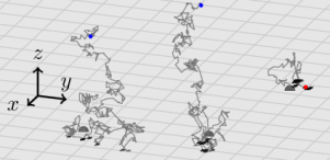
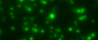
(a) Particles’ motion model	(b) Typical observation

Fig. 1: (a) Visualization, at a particle level, of the proposed physical data model. Three particles, each secreted by a different cell (dark gray) immobilized on the plane (light gray), follow a Brownian motion. When they hit the plane, they might bind to it (adsorption; black marks). After a time, they may disassociate (desorption) and continue their Brownian motion. At the end of the experiment, i.e., at time $T$, they may be free (blue dots) and thus not imaged, or bound to the surface (red dot) and thus contribute to the final image. (b) Example section of an image observation from a Fluorospot assay. FITC dye, marking IFN-$\gamma$ molecules, emitting $512~{}\mathrm{nm}$ fluorescence. Image captured by an RGB camera.

From a macroscopic point of view, this model can be expressed in terms of the time-varying concentration of particles that move freely in $z>0$, i.e., $c(x,y,z,t)\geq 0~{}[\mathrm{m}^{-3}]$. This density follows the diffusion equation

$$\frac{\partial}{\partial t}c=D\left(\frac{\partial^{2}c}{\partial x^{2}}+\frac{\partial^{2}c}{\partial y^{2}}+\frac{\partial^{2}c}{\partial z^{2}}\right)\,,\par\addvspace{-\parskip}\ignorespaces$$ (1a)

subject to boundary conditions at $$z=0 c(x,y,z,t) t d(x,y,t)\geq 0~{}[\mathrm{m}^{-2}] s(x,y,t)\geq 0~{}[\mathrm{m}^{-2}\mathrm{s}^{-1}]$$ that express reaction, adsorption and desorption. These boundary conditions couple to the surface density of bound particles at time , i.e., , and the source density rate (SDR) of new particles generated by cells residing at surface locations, i.e., , through [5]

$$\frac{\partial}{\partial t}d=\kappa_{\mathrm{a}}c\big{|}_{z=0}-\kappa_{\mathrm{d}}d\,,$$ (1b)

and

$$-D\frac{\partial}{\partial z}c\big{|}_{z=0}=s+\kappa_{\mathrm{d}}d-\kappa_{\mathrm{a}}c\big{|}_{z=0}\,.$$ (1c)

Here, $\kappa_{\mathrm{a}}~{}[\mathrm{m}\mathrm{s}^{-1}]$, $\kappa_{\mathrm{d}}~{}[\mathrm{s}^{-1}]$, and $D~{}[\mathrm{m}^{2}\mathrm{s}^{-1}]$ are physical parameters characterizing the surface’s adsorption and desorption rates and the medium’s diffusion constant, respectively. More on the generality and assumptions of this model can be found in [1, 2, 3, 4, 5, 6]. Note that $s(x,y,t)$ is spatially sharp and sparse, because particles are only released from locations occupied by cells, but also temporally continuous, because cells are immobilized throughout the experiment.

In [6], we prove that the luminosity function of the captured image, i.e., the observation $d_{\mathrm{obs}}(x,y)$, can be expressed up to a constant of proportionality as

$$d_{\mathrm{obs}}(x,y)=d(x,y,T)=\int_{0}^{\sigma_{\max}}g_{\sigma}(x,y)*a(x,y,\sigma)\mathrm{d}\sigma,$$ (2)

where $g_{\sigma}$ is a 2D isotropic Gaussian kernel of standard variation $\sigma$, $\sigma_{\max}=\sqrt{2DT}$ and $*$ represents spatial convolution. $a(x,y,\sigma)\geq 0$ for $\sigma\geq 0$ is a new quantity that we name post adsorption-desorption source density rate (PSDR), and that can be expressed as

$$a(x,y,\sigma)=\frac{\sigma}{D}\int_{\frac{\sigma^{2}}{2D}}^{T}s(x,y,T-\eta)\,\varphi\!\left(\frac{\sigma^{2}}{2D},\eta\right)\mathrm{d}\eta\,.$$ (3)

The PSDR expresses an equivalent SDR where the effect of adsorption and desorption has been summarized. Moreover, the PSDR is expressed as a function of the length $\sigma$ each of the particles has traveled from the site they were released, as opposed to the SDR, which is a function of the time at which each particle was released. In [7], we prove that $\varphi(\tau,t)$ in (3) is given by

$$\varphi(\tau,t)=i_{[0,t)}(\tau)\sum_{j=1}^{\infty}\phi^{j*}(\tau)p\left[j-1;\kappa_{\mathrm{d}}(t-\tau)\right]\,,$$ (4)

for $0\leq\tau\leq t$, $\forall t\leq T$. This function expresses the probabilistic relation between the total time in free motion $\tau$ and the time $t$ at which a particle is found bound. In (4), we have that $p[j;\lambda]$ is the probability mass function of a Poisson random variable with mean $\lambda\geq 0$ evaluated at $j\in\mathbb{N}$, $i_{[0,t)}(\tau)$ is the $(0,1)$-indicator function of the set $[0,t)$,

$$\phi(\tau)=\frac{\kappa_{\mathrm{a}}}{\sqrt{\pi D\tau}}-\frac{\kappa_{\mathrm{a}}^{2}}{D}\mathrm{erfcx}\left(\kappa_{\mathrm{a}}\sqrt{\frac{\tau}{D}}\right)\,,$$

and $\phi^{j*}(\tau)=(\overbrace{\phi*\cdots*\phi}^{j})(\tau)$ is $\phi$’s $j$-th convolutional product. Here, $\mathrm{erfcx}(x)$ is the scaled-complementary error function. For more on the generality of this observation model and how it is affected by hardware impairments such as optical blur or additive noise, see [7].

For the purpose of cell detection, it is relevant to note that $a(x,y,\sigma)$ contains the same spatial information that $s(x,y,t)$ does, because the operation to obtain $a(x,y,\sigma)$ from $s(x.y,t)$ (3) is only a convolution in the temporal dimension, which leaves spatial dependence unchanged. Consequently, $a(x,y,\sigma)$ is also spatially sharp and sparse, indicating where active cells lie. Inverting (2) to obtain the PSDR, then, is a reasonable procedure for cell detection. Moreover, recovering the PSDR also provides a representation of the amount of particles released from each cell location. For the purpose of understanding spot formation, one can simply picture the response of the observation model (2) to a spatially sharp, temporally continuous $s(x,y,t)$. This reveals that spots that are generated by active cells will always be monotone and circularly invariant. For the purpose of synthetic data generation, note that (2), (3) and (4) provide all the information needed to generate a synthetic image observation from an arbitrary SDR $s(x,y,t)$ and some physical parameters $\kappa_{\mathrm{a}},\kappa_{\mathrm{d}},D$ and $T$.

In conclusion, the novel observation model (2) allows for a new understanding of the spot formation process, but also provides natural analysis and synthesis strategies.

3 Methodology

3.1 Inverse Problem

In [6], we derive a procedure for inverting the observation model (2) in function spaces by using group-sparsity regularization and the accelerated proximal gradient (APG) algorithm (also known as FISTA). In [7], we propose a discretization and approximation of that algorithm. This discretized algorithm obtains a discrete approximation $\tilde{a}\in\operatorname{\mathbb{T}_{+}}\left(M,N,K\right)$ of $a(x,y,\sigma)\geq 0$ in (3) from a discrete image observation $\tilde{d}_{\mathrm{obs}}\in\operatorname{\mathbb{T}_{+}}\left(M,N\right)$. Here, $\operatorname{\mathbb{T}_{+}}\left(q_{1},q_{2},\dots,q_{Q}\right)$ is the space of element-wise non-negative tensors (or matrices) of dimension $q_{1}\times q_{2}\times\dots\times q_{Q}$, $M$ and $N$ are the number of pixels in each spatial direction, and $K$ is the number of discretization points used for the $\sigma$-dimension.

 

0:   An initial $\tilde{a}^{(0)}\in\operatorname{\mathbb{T}}\left(M,N,K\right)$, a discrete image observation $\tilde{d}_{\mathrm{obs}}\in\operatorname{\mathbb{T}}\left(M,N\right)$  

0:  

  $\tilde{b}^{(0)}\leftarrow\tilde{a}^{(0)}$, $i\leftarrow 0$

  repeat

     $i\leftarrow i+1$

     $\displaystyle\tilde{d}^{(i)}\leftarrow\sum_{k=1}^{K}\tilde{g}_{k}\circledast\tilde{b}^{(i-1)}_{k}-\tilde{d}_{\mathrm{obs}}$

     for  $k=1$ to $K$ do

        $\displaystyle\tilde{a}_{k}^{(i)}\leftarrow\left[\tilde{b}_{k}^{(i-1)}-\eta\tilde{g}_{k}\circledast\left[\tilde{w}^{2}\odot\tilde{d}^{(i)}\right]\right]_{+}$

     end for

     $\displaystyle\tilde{p}\leftarrow\left(1-\frac{\eta}{2}\lambda\left[\sqrt{\sum_{k=1}^{K}\left(\tilde{a}^{(i)}_{k}\right)^{2}}\right]^{-1}\right)_{+}$

     for  $k=1$ to $K$ do

        $\displaystyle\tilde{a}_{k}^{(i)}\leftarrow\tilde{p}\odot\tilde{a}_{k}^{(i)}$

     end for

     $\tilde{b}^{(i)}\leftarrow\tilde{a}^{(i)}+\alpha(i)\left(\tilde{a}^{(i)}-\tilde{a}^{(i-1)}\right)$

  until  convergence

  $\tilde{a}_{\mathrm{opt}}\leftarrow\tilde{a}^{(i)}$

    

Fig. 2: APG algorithm to obtain $\tilde{a}$. Lines 4 and 6 optimize the data fidelity term, while Lines 8 and 10 optimize the regularizer. The sequence $\alpha(i)$ can be that in [16] or that in [17], $\eta=\tilde{\sigma}_{\max}^{-1}/\max|\tilde{w}_{m,n}|^{2}$ is the algorithm’s fixed step size, $\circledast$ represents discrete size-preserving zero-padded convolution, and matrix products ($\odot$) and powers are element-wise.

Fig. 2 specifies a simplified case of this discrete algorithm. The $\tilde{g}_{k}$s are discrete rank-$1$ convolutional kernels formed by approximating finite integrals of Gaussian functions with respect to their standard deviation and spatial coordinates (see $g_{k}^{\mathrm{b1r}}$ in [7] for details), and the $\tilde{a}_{k}$s are cuts of $\tilde{a}$ in the $k$-dimension, i.e. $\tilde{a}_{k}\in\operatorname{\mathbb{T}_{+}}\left(M,N\right)$. Moreover, $\tilde{\sigma}_{\max}=\sigma_{\max}/\Delta_{\mathrm{pix}}$, where $\Delta_{\mathrm{pix}}$ is the length of a pixel’s side, and $\tilde{w}\in\operatorname{\mathbb{T}_{+}}\left(M,N\right)$ and $\lambda\geq 0$ are user parameters. In particular, the algorithm in Fig. 2 solves the finite-dimensional optimization problem

$$\min_{\tilde{a}}\left\{\left\|\tilde{w}\odot\!\left(\tilde{d}_{\mathrm{obs}}\!-\!\sum_{k=1}^{K}\tilde{g}_{k}\circledast\tilde{a}_{k}\right)\right\|_{2}^{2}\!+\!\lambda\sum_{m,n}\!\left\|\tilde{a}_{m,n}\right\|_{2}\right\}$$ (5)

subject to $\tilde{a}\in\operatorname{\mathbb{T}_{+}}\left(M,N,K\right)$, where the $\tilde{a}_{m,n}$s are cuts of $\tilde{a}$ in the spatial dimensions, i.e. $\tilde{a}_{m,n}\in\mathbb{R}^{K}$. This optimization problem can be proven to approximate the one proposed in [6]. The first term in (5) is a weighted norm used as a data-fidelity cost function with respect to a discretization of the observation model (2). The second term in (5) is a regularizer that promotes both spatial sparsity and continuity through the $k$s, i.e., a group-sparsity regularizer that induces a group behavior [18] for all the components in $\tilde{a}$ representing a certain location. The effect of this regularizer is tweaked by the regularization parameter $\lambda$, which is set larger (or lower) to increase (or decrease) selectivity.

3.2 Detection and performance evaluation

In the context of image-based immunoassays, a cell detector generally provides tuples $\left\{(\mathbf{r}_{l},p_{l})\right\}_{l=1}^{L}$, where $\mathbf{r}_{l}\in\mathbb{R}_{+}^{2}$ is a position in pixel-based coordinates and $p_{l}\geq 0$ is a non-negative number proportional to the confidence assigned to the specific detection, i.e. a pseudo-likelihood. This is done so that researchers can threshold detections by the pseudo-likelihood to match their criteria.

In our specific case, we use the estimated discrete PSDR $\tilde{a}$ obtained from the algorithm in Fig. 2 to build an image $\tilde{p}=\sqrt{\sum_{k}\tilde{a}^{2}_{k}}$. Then, we consider the pixel positions of its regional maxima as detections, and the pixel values at those positions as the respective pseudo-likelihoods. This specific $\tilde{p}$ expresses the importance of each detection with respect to the group-sparsity regularizer in (5).

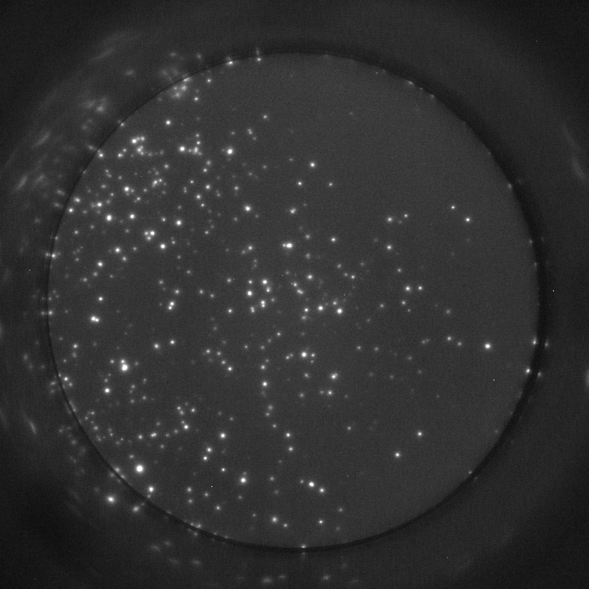
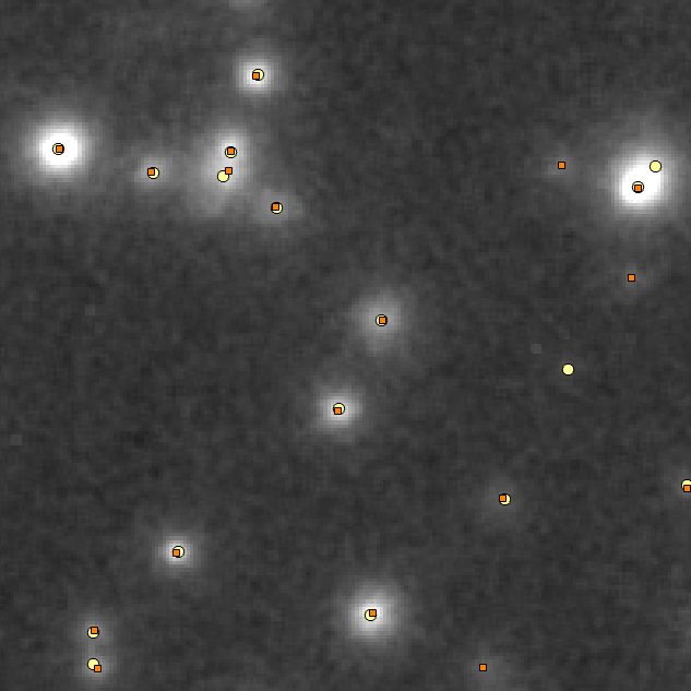
Fig. 3: To the left, grayscale image representation of the data, with increased luminosity. To the right, cell detection results (yellow circles) and human expert labeling (orange squares) for a specific section.

To evaluate the performance of our detector when ground-truth data is available, we pick the threshold for the pseudo-likelihoods $p_{l}$ that yields the best F1-score given the ground-truth data. In this manner, we hope to emulate the threshold the human expert would have chosen. The F1-score is a number in the range $[0,1]$ that expresses a compromise between precision and recall, i.e.,

$$\mathrm{pre}=\frac{\mathrm{TP}}{\mathrm{TP}+\mathrm{FP}},\,\mathrm{rec}=\frac{\mathrm{TP}}{\mathrm{TP}+\mathrm{FN}},\mbox{ and }\mathrm{F1}=\frac{2\,\mathrm{pre}\cdot\mathrm{rec}}{\mathrm{pre}+\mathrm{rec}},\,$$

with $\mathrm{TP}$, $\mathrm{FP}$ and $\mathrm{FN}$ the numbers of true and false positives and false negatives, respectively. These quantities are obtained by matching the detections to ground-truth cell positions in decreasing order of pseudo-likelihood with a tolerance of $3~{}\mathrm{pixels}$.

4 Real-Data Example

We analyzed a real Fluorospot image for which human expert labeling was available. This image was obtained by using FITC dye as a marker for some relevant analyte, and was captured by an RGB sensor that yielded a $2048\times 2048$ raw image with a dynamic range of $16~{}\mathrm{bits}$. The data was subject to a Bayer filter, i.e., neighboring pixels exhibited different sensitivities to light intensity at the FITC wavelength ($512~{}\mathrm{nm}$). To compensate this difference, we weighted each pixel correspondingly to estimate the luminosity, and used $\tilde{w}$ to weight the prediction error at each pixel according to its sensitivity. Furthermore, we selected the area that comprised the well manually, and fixed $\tilde{w}=0$ for all points outside it.

We used the algorithm in Fig. 2 with $M=N=2048$, $K=6$, $\lambda=4000$ and the sequence $\alpha(i)$ proposed in [16]. The underlying parameters $\sigma_{k}$ (see [7]) were set to $\{2,15,20,30,40,50,70\}$. We run the algorithm for 10000 iterations, which were more than those needed for convergence. The resulting F1-Score was $0.9$ with precision $0.92$ and recall $0.88$. On the left panel of Figure 3, we show a grayscale representation of the image under study, while on the right panel, we show both the detections proposed by the human expert (orange squares) and the ones proposed by our algorithm (yellow circles), on a specific section of the image.

In our opinion, both sets of detections are of comparable quality, with our algorithm being more precise in terms of cell locations and the human labeler obtaining higher recall for isolated cells. However, one has to take into account that the detections obtained by our algorithm have been thresholded to match the criteria of this specific expert, and thus, the absence of weaker spots in the set of detections can be explained by inconsistent inclusion criteria in the human labeling. A final relevant difference between the two sets of detections is that our algorithm uses the observation model to evaluate the whole shape of spots in terms of possible cells, instead of mainly relying on local luminosity. Hence, the algorithm includes detections that are weaker but fit the shape of cell-generated spots, as the apparent false positive in the middle-right region of the image. This also results in the correct decomposition of clusters of cells, as it is clearly the case of the large spot in the upper-right region of the image.

The results reported here are coherent with the extensive quantitative study on synthetic data we present in [7], which additionally suggests robustness both to additive noise and to changes in the regularization parameter $\lambda$, as well as dominance over simpler deconvolution approaches.

5 Conclusions

In this paper, we have analyzed the PDE behind some image-based immunoassays, i.e. a reaction-diffusion-adsorption-desorption equation. From this analysis, we have obtained a novel observation model for these assays. Then, we have presented the insights on the process of spot formation this observation model entails, and we have used them to propose a novel analysis algorithm. Finally, we have exemplified the use of this algorithm on real data, obtaining results that are quantitatively close and qualitatively comparable to those generated by a human expert.

References

- [1] B. Christoffer Lagerholm and Nancy L. Thompson, “Theory for ligand rebinding at cell membrane surfaces,” Biophysical Journal, vol. 74, no. 3, pp. 1215–1228, 1998.
- [2] Alena M. Lieto, B. Christoffer Lagerholm, and Nancy L. Thompson, “Lateral diffusion from ligand dissociation and rebinding at surfaces,” Langmuir, vol. 19, no. 5, pp. 1782–1787, 2003.
- [3] Alexander M. Berezhkovskii, Lazaros Batsilas, and Stanislav Y. Shvartsman, “Ligand trapping in epithelial layers and cell cultures,” Biophysical Chemistry, vol. 107, no. 3, pp. 221–227, 2004.
- [4] Ianik Plante and Francis A. Cucinotta, “Model of the initiation of signal transduction by ligands in a cell culture: Simulation of molecules near a plane membrane comprising receptors,” Phys. Rev. E, vol. 84, pp. 051920, Nov. 2011.
- [5] Alexey Y. Karulin and Paul V. Lehmann, Handbook of ELISPOT: Methods and protocols, chapter 11, pp. 125–143, Springer New York, 2nd edition, 2012.
- [6] Pol del Aguila Pla and Joakim Jaldén, “Cell detection by functional inverse diffusion and group sparsity – Part I: Theory,” arXiv, 2017, Available at: arXiv:1710.01604v1.
- [7] Pol del Aguila Pla and Joakim Jaldén, “Cell detection by functional inverse diffusion and group sparsity – Part II: Practice,” arXiv, 2017, Available at: arXiv:1710.01622v1.
- [8] Cecil C. Czerkinsky, Lars Åke Nilsson, Håkan Nygren, Örjan Ouchterlony, and Andrej Tarkowski, “A solid-phase enzyme-linked immunospot (ELISPOT) assay for enumeration of specific antibody-secreting cells,” Journal of Immunological Methods, vol. 65, no. 1, pp. 109–121, 1983.
- [9] Agnès Gazagne, Emmanuel Claret, John Wijdenes, Hans Yssel, François Bousquet, Eric Levy, Philippe Vielh, Florian Scotte, Thierry Le Goupil, Wolf H. Fridman, and Eric Tartour, “A Fluorospot assay to detect single T lymphocytes simultaneously producing multiple cytokines,” Journal of Immunological Methods, vol. 283, no. 1–2, pp. 91–98, 2003.
- [10] Tomas Dillenbeck, Eva Gelius, Jenny Fohlstedt, and Niklas Ahlborg, “Triple cytokine Fluorospot analysis of human antigen-specific IFN-, IL-17A and IL-22 responses,” Cells, vol. 3, no. 4, pp. 1116–1130, Nov. 2014.
- [11] Paola Martinez-Murillo, Lotta Pramanik, Christopher Sundling, Kjell Hultenby, Per Wretenberg, Mats Spångberg, and Gunilla B. Karlsson Hedestam, “CD38 and CD31 double-positive cells comprise the functional antibody-secreting plasma cell compartment in primate bone marrow,” Frontiers in Immunology, vol. 7, pp. 242, June 2016.
- [12] T. Meier, H.-P. Eulenbruch, P. Wrighton-Smith, G. Enders, and T. Regnath, “Sensitivity of a new commercial enzyme-linked immunospot assay (T spot-tb) for diagnosis of tuberculosis in clinical practice,” European Journal of Clinical Microbiology and Infectious Diseases, vol. 24, no. 8, pp. 529–536, 2005.
- [13] “High-throughput detection method for human papilloma virus (HPV) neutralizing antibodies,” Sept. 2015, CN Patent App. CN 201,510,346,407.
- [14] Jonathan A. Rebhahn, Courtney Bishop, Anagha A. Divekar, Katty Jiminez-Garcia, James J. Kobie, F. Eun-Hyung Lee, Genny M. Maupin, Jennifer E. Snyder-Cappione, Dietmar M. Zaiss, and Tim R. Mosmann, “Automated analysis of two- and three-color fluorescent ELISPOT (Fluorospot) assays for cytokine secretion,” Computer Methods and Programs in Biomedicine, vol. 92, no. 1, pp. 54–65, 2008.
- [15] Ihor Smal, Marco Loog, Wiro Niessen, and Erik Meijering, “Quantitative comparison of spot detection methods in fluorescence microscopy,” IEEE Transactions on Medical Imaging, vol. 29, no. 2, pp. 282–301, Feb. 2010.
- [16] Amir Beck and Marc Teboulle, “A fast iterative shrinkage-thresholding algorithm for linear inverse problems,” SIAM Journal on Imaging Sciences, vol. 2, no. 1, pp. 183–202, 2009.
- [17] Antonin Chambolle and Charles Dossal, “On the convergence of the iterates of the fast iterative shrinkage/thresholding algorithm,” Journal of Optimization Theory and Applications, vol. 166, no. 3, pp. 968–982, 2015.
- [18] Ming Yuan and Yi Lin, “Model selection and estimation in regression with grouped variables,” Journal of the Royal Statistical Society: Series B (Statistical Methodology), vol. 68, no. 1, pp. 49–67, 2006.