Accelerating the Sinkhorn-Knopp iteration by Arnoldi-type methods

Abstract

It is shown that the problem of balancing a nonnegative matrix by positive diagonal matrices can be recast as a constrained nonlinear multiparameter eigenvalue problem. Based on this equivalent formulation some adaptations of the power method and Arnoldi process are proposed for computing the dominant eigenvector which defines the structure of the diagonal transformations. Numerical results illustrate that our novel methods accelerate significantly the convergence of the customary Sinkhorn-Knopp iteration for matrix balancing in the case of clustered dominant eigenvalues.

1 Introduction

Many important types of data, like text, sound, event logs, biological sequences, can be viewed as graphs connecting basic data elements. Networks provide a powerful tool for describing the dynamic behavior of systems in biology, computer science, information engineering. Networks and graphs are generally represented as very large nonnegative matrices describing either the network topology, quantifying certain attributes of nodes or exhibiting the correlation between certain node features. Among the challenging theoretical and computational problems with these matrices there are the balancing/scalability issues.

The Sinkhorn-Knopp (SKK) balancing problem can be stated as follows: Given a nonnegative matrix $A\in\mathbb{R}^{n\times n}$ $(A\geq 0)$, find if they exist two nonnegative diagonal matrices $D_{1},D_{2}\in\mathbb{R}^{n\times n}$ such that $S=D_{1}AD_{2}$ is doubly stochastic, i.e.,

$$D_{2}A^{T}D_{1}\mbox{\boldmath$e$}=\mbox{\boldmath$e$},\quad D_{1}AD_{2}\mbox{\boldmath$e$}=\mbox{\boldmath$e$},\quad\mbox{\boldmath$e$}=\left[1,\ldots,1\right]^{T}.$$ (1)

The problem was raised in three different papers [1, 2, 3] that contain the well-known iteration for matrix balancing that bears their names. Several equilibration problems exist in which row or column norms are not equal but rather are specified by positive vectors. Variants of the SKK problem have attracted attention in various fields of pure and applied sciences including input-output analysis in economics [4], optimal transportation theory and its applications in machine learning [5], complex network analysis [6, 7], probabilistic and statistical modeling [8], optimization of traffic and telecommunication flows [9] and matrix preconditioning [10]. For a general review and summary of these applications one can see [11].

For any admissible vector $\mbox{\boldmath$v$}\in\mathbb{R}^{n}$ and any $\alpha\in\mathbb{Z}$, $\alpha\neq 0$, let $\mathcal{D}^{\alpha}(\mbox{\boldmath$v$})$ be defined as the $n\times n$ diagonal matrix with diagonal entries $d_{i}=v_{i}^{\alpha}$, $1\leq i\leq n$. Then the computation in (1) amounts to find two vectors $r$ and $c$ such that $D_{1}=\mathcal{D}(\mbox{\boldmath$r$})$ and $D_{2}=\mathcal{D}(\mbox{\boldmath$c$})$ satisfy

$$\left\{\begin{array}[]{ll}\mathcal{D}(\mbox{\boldmath$c$})A^{T}\mathcal{D}(\mbox{\boldmath$r$})\mbox{\boldmath$e$}=\mathcal{D}(\mbox{\boldmath$c$})A^{T}\mbox{\boldmath$r$}=\mathcal{D}(A^{T}\mbox{\boldmath$r$})\mbox{\boldmath$c$}=\mbox{\boldmath$e$};\\ \mathcal{D}(\mbox{\boldmath$r$})A\mathcal{D}(\mbox{\boldmath$c$})\mbox{\boldmath$e$}=\mathcal{D}(\mbox{\boldmath$r$})A\mbox{\boldmath$c$}=\mathcal{D}(A\mbox{\boldmath$c$})\mbox{\boldmath$r$}=\mbox{\boldmath$e$}\end{array}\right.$$

When $A$ is symmetric we can determine $\mbox{\boldmath$r$}=\mbox{\boldmath$c$}=\mbox{\boldmath$z$}$ to satisfy $\mathcal{D}(A\mbox{\boldmath$z$})\mbox{\boldmath$z$}=\mathcal{D}(\mbox{\boldmath$z$})A\mbox{\boldmath$z$}=\mbox{\boldmath$e$}$. In [2] the authors proposed the following fixed point iteration –called Sinkhorn-Knopp (SKK) iteration– for computing the desired vectors $r$ and $c$:

$$\left\{\begin{array}[]{ll}\mbox{\boldmath$c$}_{k+1}=\mathcal{D}^{-1}(A^{T}\mbox{\boldmath$r$}_{k})\mbox{\boldmath$e$};\\ \mbox{\boldmath$r$}_{k+1}=\mathcal{D}^{-1}(A\mbox{\boldmath$c$}_{k+1})\mbox{\boldmath$e$}\end{array}\right.$$ (2)

In the symmetric case the SKK iteration reduces to

$$\mbox{\boldmath$z$}_{k+1}=\mathcal{D}^{-1}(A\mbox{\boldmath$z$}_{k})\mbox{\boldmath$e$}$$ (3)

or, equivalently, by setting $1./\mbox{\boldmath$z$}_{k}=\mbox{\boldmath$x$}_{k}$ with the assumption $1/0=+\infty$,

$$\mbox{\boldmath$x$}_{k+1}=1./\mbox{\boldmath$z$}_{k+1}=A\mbox{\boldmath$z$}_{k}=A(1./\mbox{\boldmath$x$}_{k}).$$ (4)

The SKK iterations (2),(3),(4) have been rediscovered several times in different applicative contexts. Related methods are the RAS method [4] in economics, the iterative proportional fitting procedure (IPFP) in statistics and Kruithof’s projection scheme [9] in optimization.

A common drawback of all these iterative algorithms is the slow convergence behavior exhibited even in deceivingly simple cases. To explain this performance gap we observe that the equations in (2) can be combined to get

$$\mbox{\boldmath$c$}_{k+1}=\mathcal{D}^{-1}(A^{T}\mathcal{D}^{-1}(A\mbox{\boldmath$c$}_{k})\mbox{\boldmath$e$})\mbox{\boldmath$e$},\quad k\geq 0,$$ (5)

which can be expressed componentwise as

$$(\mbox{\boldmath$c$}_{k+1})_{s}=\left(\sum_{m=1}^{n}a_{m,s}\left(\sum_{\ell=1}^{n}a_{m,\ell}(\mbox{\boldmath$c$}_{k})_{\ell}\right)^{-1}\right)^{-1},\quad 1\leq s\leq n,\ k\geq 0.$$

This means that (5) is equivalent to the fixed point iteration

$$\mbox{\boldmath$c$}_{k+1}=T(\mbox{\boldmath$c$}_{k}),\quad T(\mbox{\boldmath$x$}_{s})=\left(\sum_{m=1}^{n}a_{m,s}\left(\sum_{\ell=1}^{n}a_{m,\ell}\mbox{\boldmath$x$}_{\ell}\right)^{-1}\right)^{-1},$$ (6)

for solving

$$\mbox{\boldmath$x$}=T\mbox{\boldmath$x$},\quad\mbox{\boldmath$x$}\geq\mbox{\boldmath$0$},$$ (7)

where $T$ is the nonlinear operator introduced by Menon in [12, 13] and according to those papers we write $T\mbox{\boldmath$x$}=T(\mbox{\boldmath$x$})$.

Our first contribution consists of a novel formulation of the fixed point problem (7) as a constrained nonlinear multiparameter eigenvalue problem of the form

$$\mbox{\boldmath$x$}=J_{T}(\mbox{\boldmath$x$})\mbox{\boldmath$x$},\quad\mbox{\boldmath$x$}\geq\mbox{\boldmath$0$},$$ (8)

where $J_{T}(\mbox{\boldmath$z$})$ denotes the Jacobian matrix of $T$ evaluated at the point $z$. Although the proof is quite simple, to our knowledge this property has been completely overlooked in the literature even though it has several implications.

From a theoretical viewpoint, it follows that the local dynamics of the original SKK algorithm (5) can be described as a power method with perturbations [14] applied to the matrix $J_{T}(\mbox{\boldmath$x$})$ evaluated at the fixed point. Therefore the SKK iterations (2),(3),(4) inherit the pathologies of the power process in the case of clustered dominant eigenvalues of $J_{T}(\mbox{\boldmath$x$})$. A related result has appeared in [6].

Furthermore, relation (8) can also be exploited in order to speed up the computation of the Sinkhorn-Knopp vector. Acceleration methods using nonlinear solvers applied to equation (7) have been recently proposed in [15] whereas optimization strategies and descending techniques are considered in [16, 17]. In this paper we pursue a different approach by taking into account the properties of the equivalent nonlinear multiparameter eigenvalue problem (8). Krylov methods are the algorithms of choice for the computation of a few eigenvalues of largest magnitude of matrices. They have been efficiently used in information retrieval and web search engines for accelerating PageRank computations [18, 19]. In particular, Arnoldi-based methods have been proven to be efficient for achieving eigenvalue/eigenvector separation [19]. Based on this, we propose here to compute an approximation of the fixed point of $T$ by using a different fixed point iteration method of the form $\lambda_{k}\mbox{\boldmath$v$}_{k+1}=J_{T}(\mbox{\boldmath$v$}_{k})\mbox{\boldmath$v$}_{k+1}$, $k\geq 0$, where $\lambda_{k}$ is the dominant eigenvalue of $J_{T}(\mbox{\boldmath$v$}_{k})$ with corresponding normalized eigenvector $\mbox{\boldmath$v$}_{k+1}$. Each iteration amounts to approximate the dominant eigenpair of a matrix $J_{T}(\mbox{\boldmath$v$}_{k})$. Fast eigensolvers relying upon the power method and the Arnoldi process are specifically tailored to solve these problems for large-scale matrices. Numerical results show that the resulting schemes are successful attempts to accelerate the convergence of the SKK iterations in the case of clustered dominant eigenvalues of $J_{T}(\mbox{\boldmath$x$})$.

The paper is organized as follows. In Section 2 after briefly recalling the properties of the SKK fixed point iteration (6) we exploit the eigenvalue connection by devising accelerated variants of (6) using Arnoldi-type methods. The description and implementation of these variants together with numerical results are discussed in Section 3. Finally, in section 4 conclusion and some remarks on future work are given.

2 Theoretical Setup

Let us denote by $\mathcal{P},\mathcal{P}_{0}$ and $\mathcal{P}_{\infty}$ the subsets of $\bar{\mathbb{R}}^{n}$, $\bar{\mathbb{R}}=\mathbb{R}\cup\{\pm\infty\}$, defined by $\mathcal{P}=\{\mbox{\boldmath$x$}\in\mathbb{R}^{n}\colon\mbox{\boldmath$x$}\geq\mbox{\boldmath$0$}\}$, $\mathcal{P}_{0}=\{\mbox{\boldmath$x$}\in\mathbb{R}^{n}\colon\mbox{\boldmath$x$}>\mbox{\boldmath$0$}\}$ and $\mathcal{P}_{\infty}=\{\mbox{\boldmath$x$}\in\bar{\mathbb{R}}^{n}\colon\mbox{\boldmath$x$}\geq\mbox{\boldmath$0$}\}$, respectively. For the sake of simplicity we assume that $A\in\mathbb{R}^{n\times n}$ is a matrix with all positive entries, that is, $A>0$. Results for more general indecomposable nonnegative matrices are obtained by a continuity argument using the perturbative analysis introduced in [13] (see also Section 6.2 in [20]). Numerical evidences shown in Section 3 indicate that our approach also works in the more general setting.

Arithmetic operations are generalized over the nonnegative extended real line $[0,+\infty]\subset\bar{\mathbb{R}}$ by setting [13] $1/0=\infty$, $1/\infty=0$, $\infty+\infty=\infty$, $0\cdot\infty=0$, $a\cdot\infty=\infty$ if $a>0$, where $\infty=+\infty$. Under these assumptions we can introduce the nonlinear operators defined as follows:

1. $U\colon\mathcal{P}_{\infty}\rightarrow\mathcal{P}_{\infty}$, $U\mbox{\boldmath$x$}=1./\mbox{\boldmath$x$}$;

2. $S\colon\mathcal{P}_{\infty}\rightarrow\mathcal{P}_{\infty}$, $S\mbox{\boldmath$x$}=UA\mbox{\boldmath$x$}$;

3. $T\colon\mathcal{P}_{\infty}\rightarrow\mathcal{P}_{\infty}$, $T\mbox{\boldmath$x$}=UA^{T}UA\mbox{\boldmath$x$}$.

In this way it can be easily noticed that $T$ is the same as the operator introduced in (6) and, therefore, the Sinkhorn-Knopp problem for the matrix $A$ reduces to computing the fixed points of $T$, that is, the vectors $\mbox{\boldmath$x$}\in\mathcal{P}_{\infty}$ such that

$$\mbox{\boldmath$x$}=T\mbox{\boldmath$x$}=UA^{T}UA\mbox{\boldmath$x$},\quad\mbox{\boldmath$x$}\in\mathcal{P}_{\infty}.$$ (9)

Summing up the results stated in [12, 13] we obtain the following theorem concerning the existence and the uniqueness of the desired fixed point.

Theorem 2.1.

Let $A\in\mathbb{R}^{n\times n}$ be a matrix with all positive entries. Then $\forall\mbox{\boldmath$u$}\in\mathcal{P}\setminus\{\mbox{\boldmath$0$}\}$ we have $\sup\{\lambda\colon T\mbox{\boldmath$u$}\geq\lambda\mbox{\boldmath$u$}\}\leq 1$. Moreover, $T$ has a distinct eigenvalue equal to $1$ with a unique (except for positive scalar multiples) corresponding eigenvector $\mbox{\boldmath$x$}\in\mathcal{P}_{0}$.

The basic SKK algorithm proceeds to approximate the eigenvector $\mbox{\boldmath$x$}\in\mathcal{P}_{0}$ by means of the fixed point iteration

$$\left\{\begin{array}[]{ll}\mbox{\boldmath$x$}^{(0)}\in\mathcal{P}_{0};\\ \mbox{\boldmath$x$}^{(k+1)}=T\mbox{\boldmath$x$}^{(k)},\quad k\geq 0\end{array}\right.$$ (10)

The iteration is shown to be globally convergent since $T$ is a contraction for the Hilbert metric associated to the cone $\mathcal{P}$. [21, 22].

Theorem 2.2.

For any $\mbox{\boldmath$x$}^{(0)}\in\mathcal{P}_{0}$ there exists $\gamma=\gamma(\mbox{\boldmath$x$}^{(0)})\in\mathbb{R}$, $\gamma>0$, such that

$$\lim_{k\rightarrow\infty}\mbox{\boldmath$x$}^{(k)}=\gamma\mbox{\boldmath$x$}.$$

The convergence is linear and the rate depends on the second singular value of the doubly stochastic matrix $P=\mathcal{D}(S\mbox{\boldmath$x$})A\mathcal{D}(\mbox{\boldmath$x$})$. We have the following [6].

Theorem 2.3.

Let $\mbox{\boldmath$x$}\in\mathcal{P}_{0}$ denote the limit of the sequence $\{\mbox{\boldmath$x$}^{(k)}\}_{k\in\mathbb{N}}$ generated according to (10). Then the matrix $\Sigma=\mathcal{D}(S\mbox{\boldmath$x$})A\mathcal{D}(\mbox{\boldmath$x$})$ is doubly stochastic and, moreover, if $\sigma_{2}$ is the second largest singular value of $\Sigma$ it holds

$$\parallel\mbox{\boldmath$x$}^{(k+1)}-\mbox{\boldmath$x$}\parallel_{2}\leq\sigma_{2}^{2}\parallel\mbox{\boldmath$x$}^{(k)}-\mbox{\boldmath$x$}\parallel_{2}+o\left(\parallel\mbox{\boldmath$x$}^{(k)}-\mbox{\boldmath$x$}\parallel_{2}\right),\quad k\geq 0.$$

The convergence can be very slow in the case of nearly decomposable matrices. The following definition is provided in [23, 24].

Definition 2.4.

For a given $\epsilon>0$, the matrix $A\in\mathbb{R}^{n\times n}$ is $\epsilon$-nearly decomposable if there exist $E\in[0,1]^{n\times n}$ and a permutation matrix $P$ such that $PAP^{T}=\hat{A}+\epsilon E$ where $\hat{A}$ is block triangular with square diagonal blocks.

The relevance of nearly decomposable matrices for the study of dynamic systems in economics has been examined by Simon and Ando [25]. The role of near decomposability in queuing and computer system applications has been discussed in [26]. For a general overview of the properties of nearly decomposable graphs and networks with applications in data science and information retrieval one can see [27].

Example 2.5.

Let $A=\displaystyle\left[\begin{array}[]{cc}1-\epsilon&\epsilon\\ \epsilon&1-\epsilon\end{array}\right]$, $0<\epsilon<1$ be a doubly stochastic matrix. The vector $\mbox{\boldmath$x$}=[1,1]^{T}$ provides a solution of the SKK scaling problem. The singular values of the matrix $A=\mathcal{D}(S\mbox{\boldmath$x$})A\mathcal{D}(\mbox{\boldmath$x$})$ satisfy $\sigma_{1}=1$ and $\sigma_{2}=|1-2\epsilon|$. For the matrix $A=\displaystyle\left[\begin{array}[]{cc}1&\epsilon\\ 1&1\end{array}\right]$, $\epsilon>0$, the SKK iteration (10) is convergent but the number of iterations grows exponentially as $\epsilon$ becomes small. In Table 1 we show the number of iterations performed by Algorithm 1 in Section 3 applied to the matrix $A$ with the error tolerance $\tau=1.0e-8$.

Table 1: Number of SKK iterations $ItN$ for different values of $\epsilon=10^{-k}$

$k$	1	2	3	4	5	6	7	8	9	10
$ItN$	16	46	132	391	1139	3312	9563	27360	77413	216017

The local dynamics of (10) depend on the properties of the Jacobian matrix evaluated at the fixed point. By using the chain rule for the composite function we obtain that

$$J_{T}(\mbox{\boldmath$z$})=J_{UA^{T}UA}(\mbox{\boldmath$z$})=J_{U}(A^{T}UA\mbox{\boldmath$z$})\cdot J_{A}^{T}(UA\mbox{\boldmath$z$})\cdot J_{U}(A\mbox{\boldmath$z$})\cdot J_{A}(\mbox{\boldmath$z$}).$$

Since $J_{U}(\mbox{\boldmath$z$})=-\operatorname{\mathcal{D}}^{-2}(\mbox{\boldmath$z$})$ we find that

$$J_{T}(\mbox{\boldmath$z$})=\operatorname{\mathcal{D}}^{2}(T\mbox{\boldmath$z$})\cdot A^{T}\cdot\operatorname{\mathcal{D}}^{2}(S\mbox{\boldmath$z$})A.$$ (11)

The next result gives a lower bound for the spectral radius of $J_{T}(\mbox{\boldmath$z$})$ for $\mbox{\boldmath$z$}\in\mathcal{P}_{0}$.

Theorem 2.6.

For any given fixed $\mbox{\boldmath$z$}\in\mathcal{P}_{0}$ the spectral radius of $J_{T}(\mbox{\boldmath$z$})$ satisfies $\rho(J_{T}(\mbox{\boldmath$z$}))\geq 1$.

Proof.

Let us denote $G=\operatorname{\mathcal{D}}(T\mbox{\boldmath$z$})\cdot A^{T}\cdot\operatorname{\mathcal{D}}(S\mbox{\boldmath$z$})$. It holds

$$J_{T}(\mbox{\boldmath$z$}) =\operatorname{\mathcal{D}}^{2}(T\mbox{\boldmath$z$})\cdot A^{T}\cdot\operatorname{\mathcal{D}}^{2}(S\mbox{\boldmath$z$})A$$

$$=\operatorname{\mathcal{D}}(T\mbox{\boldmath$z$})\cdot G\cdot G^{T}\operatorname{\mathcal{D}}^{-1}(T\mbox{\boldmath$z$}),$$

and, hence $J_{T}(\mbox{\boldmath$z$})$ and $G\cdot G^{T}$ are similar. Now observe that

$$G\mbox{\boldmath$e$}=\operatorname{\mathcal{D}}(T\mbox{\boldmath$z$})\cdot A^{T}\cdot\operatorname{\mathcal{D}}(S\mbox{\boldmath$z$})\mbox{\boldmath$e$}=\operatorname{\mathcal{D}}(T\mbox{\boldmath$z$})\cdot A^{T}UA\mbox{\boldmath$z$}=\mbox{\boldmath$e$}.$$

It follows that $\parallel G\parallel_{2}\geq 1$. By using the SVD of $G$ it is found that $\sigma_{1}(G)\geq 1$ and therefore the spectral radius of $J_{T}(\mbox{\boldmath$z$})$ satisfies $\rho(J_{T}(\mbox{\boldmath$z$}))\geq 1$. ∎

If $\mbox{\boldmath$x$}=T\mbox{\boldmath$x$}$, $\mbox{\boldmath$x$}\in\mathcal{P}_{0}$, then it is worth noting that

$$J_{T}(\mbox{\boldmath$x$})=\operatorname{\mathcal{D}}^{2}(T\mbox{\boldmath$x$})\cdot A^{T}\cdot\operatorname{\mathcal{D}}^{2}(S\mbox{\boldmath$x$})A=\operatorname{\mathcal{D}}^{2}(\mbox{\boldmath$x$})\cdot A^{T}\cdot\operatorname{\mathcal{D}}^{2}(S\mbox{\boldmath$x$})A,$$

and, hence,

$$J_{T}(\mbox{\boldmath$x$})=\operatorname{\mathcal{D}}(\mbox{\boldmath$x$})\cdot P^{T}P\operatorname{\mathcal{D}}^{-1}(\mbox{\boldmath$x$}),$$

where $P$ is introduced in Theorem 2.3. This means that $J_{T}(\mbox{\boldmath$x$})$ and $F=P^{T}P$ are similar and therefore the eigenvalues of $J_{T}(\mbox{\boldmath$x$})$ are the squares of the singular values of $P$. Since $A>0$ then it is irreducible and primitive and the same holds for $P$ and a fortiori for $F$. By the Perron-Frobenius theorem it follows that the spectral radius of $J_{T}(\mbox{\boldmath$x$})$ satisfies $\rho(J_{T}(\mbox{\boldmath$x$}))=1$ and $\lambda=1$ is a simple eigenvalue of $J_{T}(\mbox{\boldmath$x$})$ with a positive corresponding eigenvector.

A characterization of such an eigenvector can be derived by the following result.

Theorem 2.7.

For each vector $\mbox{\boldmath$z$}\in\mathcal{P}_{0}$ it holds

$$T\mbox{\boldmath$z$}=J_{T}(\mbox{\boldmath$z$})\cdot\mbox{\boldmath$z$}.$$

Proof.

Let $\mbox{\boldmath$z$}\in\mathbb{R}^{n}$, $\mbox{\boldmath$z$}>\mbox{\boldmath$0$}$, then we have

$$J_{T}(\mbox{\boldmath$z$})\cdot\mbox{\boldmath$z$} =\operatorname{\mathcal{D}}^{2}(T\mbox{\boldmath$z$})\cdot A^{T}\cdot\operatorname{\mathcal{D}}^{2}(S\mbox{\boldmath$z$})A\mbox{\boldmath$z$}$$

$$=\operatorname{\mathcal{D}}^{2}(T\mbox{\boldmath$z$})\cdot A^{T}\cdot S\mbox{\boldmath$z$}$$

$$=\operatorname{\mathcal{D}}^{-2}(A^{T}S\mbox{\boldmath$z$})\cdot A^{T}\cdot S\mbox{\boldmath$z$}$$

$$=\operatorname{\mathcal{D}}^{-1}(A^{T}S\mbox{\boldmath$z$})\mbox{\boldmath$e$}$$

$$=\operatorname{\mathcal{D}}(UA^{T}UA\mbox{\boldmath$z$})\mbox{\boldmath$e$}$$

$$=T\mbox{\boldmath$z$}.$$

∎

This theorem implies that

$$\mbox{\boldmath$x$}\in\mathcal{P}_{0},\ \mbox{\boldmath$x$}=T\mbox{\boldmath$x$}\quad\iff\quad\mbox{\boldmath$x$}\in\mathcal{P}_{0},\ \mbox{\boldmath$x$}=J_{T}(\mbox{\boldmath$x$})\mbox{\boldmath$x$}$$

and therefore the eigenvector of $J_{T}(\mbox{\boldmath$x$})$ corresponding with the eigenvalue $1$ is exactly the desired solution of the SKK problem. Furthermore, the SKK iteration (10) can equivalently be written as

$$\left\{\begin{array}[]{ll}\mbox{\boldmath$x$}^{(0)}\in\mathcal{P}_{0};\\ \mbox{\boldmath$x$}^{(k+1)}=T\mbox{\boldmath$x$}^{(k)}=J_{T}(\mbox{\boldmath$x$}^{(k)})\mbox{\boldmath$x$}^{(k)},\quad k\geq 0\end{array}\right.$$ (12)

In principle one can accelerate the convergence of this iteration without improving the efficiency of the iterative method by replacing $T$ with the operator $T_{\ell}=T\circ T\circ\cdots\circ T$, $T_{1}=T$, generated from the composition ($\ell$ times) of $T$ for a certain $\ell\geq 1$. The linearized form of the resulting iteration around the fixed point $\mbox{\boldmath$x$}=T\mbox{\boldmath$x$}$, $\mbox{\boldmath$x$}\in\mathcal{P}_{0}$, is

$$\left\{\begin{array}[]{ll}\mbox{\boldmath$x$}^{(0)}\in\mathcal{P}_{0};\\ \mbox{\boldmath$x$}^{(k+1)}=J_{T}^{\ell}(\mbox{\boldmath$x$})\mbox{\boldmath$x$}^{(k)},\quad k\geq 0\end{array}\right.$$ (13)

This is the power method applied to the matrix $J_{T}^{\ell}(\mbox{\boldmath$x$})$ for the approximation of an eigenvector associated with the dominant eigenvalue $\lambda=1$. A normalized variant of (13) can be more suited for numerical computations

$$\left\{\begin{array}[]{ll}\mbox{\boldmath$x$}^{(0)}\in\mathcal{P}_{0};\\ \left\{\begin{array}[]{ll}\mbox{\boldmath$v$}^{(k+1)}=J_{T}^{\ell}(\mbox{\boldmath$x$})\mbox{\boldmath$x$}^{(k)},\\ \mbox{\boldmath$x$}^{(k+1)}=v^{(k+1)}/(\mbox{\boldmath$e$}^{T}\mbox{\boldmath$v$}^{(k+1)})\end{array}\right.,\quad k\geq 0\end{array}\right.$$ (14)

Since $\lambda=1$ is the simple dominant eigenvalue of $J_{T}(\mbox{\boldmath$x$})$ with a positive corresponding eigenvector it is well known that (14) generates sequences such that

$$\lim_{k\rightarrow\infty}\mbox{\boldmath$x$}^{(k)}=\mbox{\boldmath$x$}/(\mbox{\boldmath$e$}^{T}\mbox{\boldmath$x$}),\quad\limsup_{k\rightarrow\infty}\parallel\mbox{\boldmath$x$}^{(k)}-\mbox{\boldmath$x$}/(\mbox{\boldmath$e$}^{T}\mbox{\boldmath$x$})\parallel_{2}^{1/k}\leq\lambda_{2}^{\ell}=\sigma_{2}^{2\ell},$$

where $0\leq\lambda_{2}=\sigma_{2}^{2}<1$ is the second largest eigenvalue of $J_{T}(\mbox{\boldmath$x$})$ and $\sigma_{2}$ denotes the second largest singular value of $P$ defined as in Theorem 2.3. For practical purposes we introduce the following modified adaptation of (14) called SKK_ℓ iteration:

$$\left\{\begin{array}[]{ll}\mbox{\boldmath$x$}^{(0)}\in\mathcal{P}_{0};\\ \left\{\begin{array}[]{ll}\mbox{\boldmath$v$}^{(k+1)}=J_{T}^{\ell}(\mbox{\boldmath$x$}^{(k)})\mbox{\boldmath$x$}^{(k)},\\ \mbox{\boldmath$x$}^{(k+1)}=v^{(k+1)}/(\mbox{\boldmath$e$}^{T}\mbox{\boldmath$v$}^{(k+1)})\end{array}\right.,\quad k\geq 0\end{array}\right.$$ (15)

For $\ell=1$ SKK₁ reduces to the scaled customary SKK iteration. Under suitable assumptions we can show that SKK_ℓ generates a sequence converging to the desired fixed point.

Theorem 2.8.

Let $\{\mbox{\boldmath$x$}^{(k)}\}_{k}$ be the sequence generated by SKK_ℓ from a given initial guess $\mbox{\boldmath$x$}^{(0)}\in\mathcal{P}_{0}$. Let $\mbox{\boldmath$x$}\in\mathcal{P}_{0}$ be such that $\mbox{\boldmath$x$}=T\mbox{\boldmath$x$}$ and $\mbox{\boldmath$e$}^{T}\mbox{\boldmath$x$}=1$. Assume that:

1. $\exists\eta>0$ $\colon$ $J_{T}^{\ell}(\mbox{\boldmath$x$}^{(k)})=J_{T}^{\ell}(\mbox{\boldmath$x$})+E_{k}$, $\parallel E_{k}\parallel_{2}\leq\eta\sigma_{2}^{2\ell k}$,  $k\geq 0$;

2. $\exists\gamma>0$ $\colon$ $\parallel\prod_{k=0}^{m}J_{T}^{\ell}(\mbox{\boldmath$x$}^{(k)})\parallel_{2}\geq\gamma$,  $m\geq 0$.

Then we have

$$\lim_{k\rightarrow\infty}\mbox{\boldmath$x$}^{(k)}=\mbox{\boldmath$x$},$$

and

$$\limsup_{k\rightarrow\infty}\parallel\mbox{\boldmath$x$}^{(k)}-\mbox{\boldmath$x$}\parallel_{2}^{1/k}\leq\sigma_{2}^{2\ell}.$$

Proof.

Since $\sum_{k=0}^{\infty}\parallel E_{k}\parallel_{2}<\infty$ from Theorem 4.1 in [14] we obtain that the matrix sequence $P_{m}=\prod_{k=0}^{m}J_{T}^{\ell}(\mbox{\boldmath$x$}^{(k)})$ is such that

$$\lim_{m\rightarrow\infty}P_{m}=\mbox{\boldmath$x$}\mbox{\boldmath$z$}^{T},\quad\mbox{\boldmath$z$}\in\mathcal{P}.$$

From Property 2 in view of the continuity of the norm it follows that $\mbox{\boldmath$z$}\neq\mbox{\boldmath$0$}$ and this implies the convergence of $\{\mbox{\boldmath$x$}^{(k)}\}_{k}$. About the rate of convergence we observe that

$$\parallel\mbox{\boldmath$x$}^{(k+1)}-\mbox{\boldmath$x$}\parallel_{2} =\parallel\frac{P_{k}\mbox{\boldmath$x$}^{(0)}}{\mbox{\boldmath$e$}^{T}P_{k}\mbox{\boldmath$x$}^{(0)}}-\mbox{\boldmath$x$}\frac{\mbox{\boldmath$z$}^{T}\mbox{\boldmath$x$}^{(0)}}{\mbox{\boldmath$z$}^{T}\mbox{\boldmath$x$}^{(0)}}\parallel_{2}$$

$$\leq\parallel\frac{P_{k}\mbox{\boldmath$x$}^{(0)}}{\mbox{\boldmath$z$}^{T}\mbox{\boldmath$x$}^{(0)}}-\mbox{\boldmath$x$}\frac{\mbox{\boldmath$z$}^{T}\mbox{\boldmath$x$}^{(0)}}{\mbox{\boldmath$z$}^{T}\mbox{\boldmath$x$}^{(0)}}\parallel_{2}+\parallel\frac{P_{k}\mbox{\boldmath$x$}^{(0)}}{\mbox{\boldmath$e$}^{T}P_{k}\mbox{\boldmath$x$}^{(0)}}-\frac{P_{k}\mbox{\boldmath$x$}^{(0)}}{\mbox{\boldmath$z$}^{T}\mbox{\boldmath$x$}^{(0)}}\parallel_{2}$$

$$\leq\frac{\parallel(P_{k}-\mbox{\boldmath$x$}\mbox{\boldmath$z$}^{T})\mbox{\boldmath$x$}^{(0)})\parallel_{2}}{|{\mbox{\boldmath$z$}^{T}\mbox{\boldmath$x$}^{(0)}}|}+\parallel P_{k}\mbox{\boldmath$x$}^{(0)}\parallel_{2}\left|\frac{\mbox{\boldmath$e$}^{T}(\mbox{\boldmath$x$}\mbox{\boldmath$z$}^{T}-P_{k}\mbox{\boldmath$)$}x^{(0)}}{\mbox{\boldmath$e$}^{T}P_{k}\mbox{\boldmath$x$}^{(0)}\mbox{\boldmath$z$}^{T}\mbox{\boldmath$x$}^{(0)}}\right|$$

which says that $\mbox{\boldmath$x$}^{(k)}$ approaches $x$ as fast as $P_{k}$ tends to $\mbox{\boldmath$x$}\mbox{\boldmath$z$}^{T}$. Again using Theorem 4.1 in [14] under our assumptions there follows that

$$\limsup_{k\rightarrow\infty}\parallel P_{k}-\mbox{\boldmath$x$}\mbox{\boldmath$z$}^{T}\parallel_{2}^{1/k}\leq\sigma_{2}^{2\ell}=\lambda_{2}^{\ell}.$$

which concludes the proof. ∎

This theorem shows that in our model the speed of convergence increases as $\ell$ increases. Also, notice that for any $\mbox{\boldmath$z$}\in\mathcal{P}_{0}$ the matrix $J_{T}(\mbox{\boldmath$z$})$ is primitive and irreducible and therefore by the Perron-Frobenius theorem its spectral radius is a dominant eigenvalue with a corresponding positive eigenvector. From Theorem 2.6 this eigenvalue is greater than or equal to 1. It follows that for large $\ell$ the iterate $\mbox{\boldmath$x$}^{(k+1)}$ provides an approximation of the positive dominant eigenvector of $J_{T}(\mbox{\boldmath$x$}^{(k)})$. This fact suggests to consider SKK_∞ as an effective method for approximating the limit vector $x$. The method performs as an inner-outer procedure. In the inner phase given the current approximation $\mbox{\boldmath$x$}^{(k)}$ of $x$ we apply the Power Method

$$\left\{\begin{array}[]{ll}\mbox{\boldmath$v$}^{(0)}=\mbox{\boldmath$x$}^{(k)};\\ \left\{\begin{array}[]{ll}\mbox{\boldmath$z$}^{(k+1)}=J_{T}(\mbox{\boldmath$x$}^{(k)})\mbox{\boldmath$v$}^{(k)},\\ \mbox{\boldmath$v$}^{(k+1)}=\mbox{\boldmath$z$}^{(k+1)}/(\mbox{\boldmath$e$}^{T}\mbox{\boldmath$z$}^{(k+1)})\end{array}\right.,\quad k\geq 0\end{array}\right.$$ (16)

until convergence to find the new approximation $\mbox{\boldmath$x$}^{(k+1)}=\mbox{\boldmath$v$}^{(\hat{k}+1)}$. Numerically this latter vector solves

$$J_{T}(\mbox{\boldmath$x$}^{(k)})\mbox{\boldmath$x$}^{(k+1)}=\theta_{k}\mbox{\boldmath$x$}^{(k+1)},\ \theta_{k}=\rho(J_{T}(\mbox{\boldmath$x$}^{(k)})),\ \mbox{\boldmath$e$}^{T}\mbox{\boldmath$x$}^{(k+1)}=1.$$ (17)

Ideally, $\theta_{k}$ would converge from above to $1$ as well as the corresponding positive eigenvector $\mbox{\boldmath$x$}^{(k+1)}$ would approach $x$; also, the convergence of the outer iteration should be superlinear.

Example 2.9.

As in Example 2.5 let $A=\displaystyle\left[\begin{array}[]{cc}1&\epsilon\\ 1&1\end{array}\right]$ with $\epsilon=1.0e-8$. In Figure 1a e 1b we illustrate the convergence history of iteration (17) applied to $A$ with starting guess $\mbox{\boldmath$x$}^{(0)}=\mbox{\boldmath$v$}^{(0)}=\left[1/2,1/2\right]^{T}$. The iterative scheme stops after 13 steps. The dominant eigenpair $(\lambda_{k},\mbox{\boldmath$v$}^{(k+1)})$ is computed by using the function eig of MatLab. In Figure 1b we show the distance between two consecutive normalized eigenvectors measured in the Hilbert metric $d_{H}(\mbox{\boldmath$u$},\mbox{\boldmath$v$})=\max_{i,j}\log\left(\displaystyle\frac{u_{i}v_{j}}{v_{i}u_{j}}\right),\ \forall\mbox{\boldmath$u$},\mbox{\boldmath$v$}\in\mathcal{P}_{0}.$

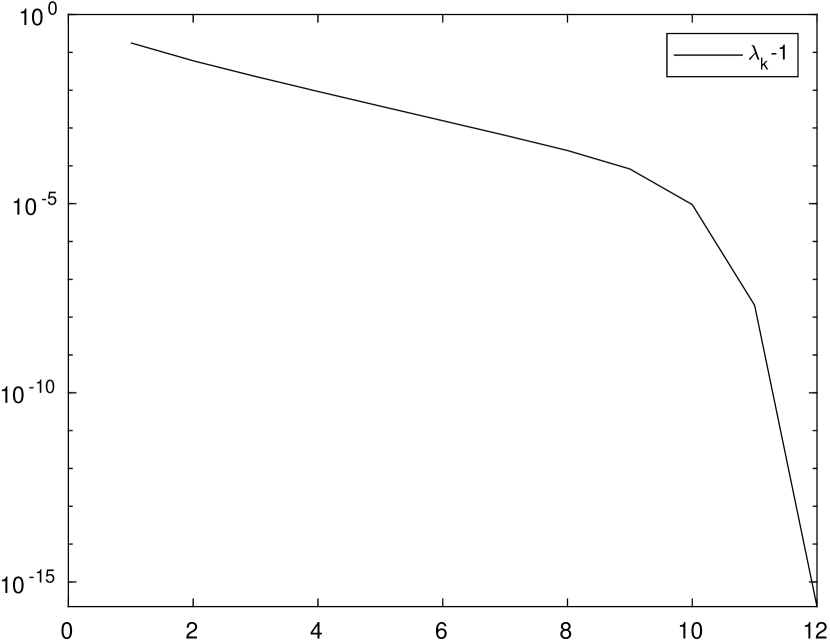
(a) Figure 1a

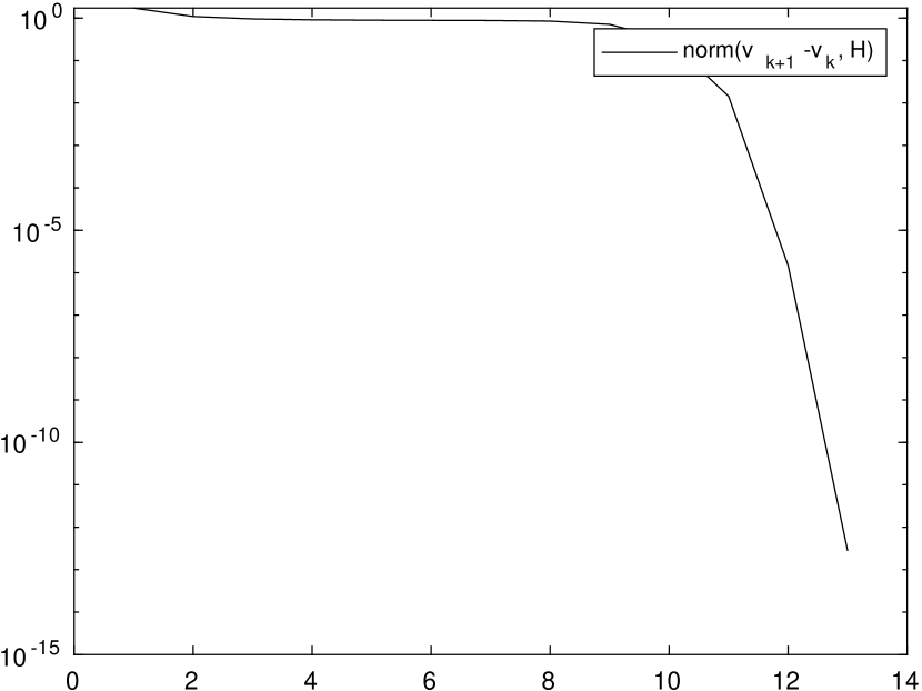
(b) Figure 1b

In principle the matrix eigenvalue problem (17) can be solved by using any reliable method. For large sparse matrices in the case of clustered eigenvalues the convergence of the inner iteration can be greatly improved by considering variants of the power method based on the Arnoldi/Krylov process for approximating a few largest eigenvalues of the matrix. In the next section the effectiveness and robustness of these methods are evaluated by numerical experiments.

3 Experimental Setup

We have tested the algorithms presented above in a numerical environment using MatLab R2018b on a PC with Intel Core i7-4790 processor. The first method to be considered is the scaled SKK iteration implemented by Algorithm 1.

Algorithm 1 Scaled SKK iteration

Input: $A\in\mathbb{R}^{n\times n}$, $A\geq 0$ and a tolerance $\tau>0$
      Output: $x$ such that $\mbox{\boldmath$x$}=T\mbox{\boldmath$x$}$, $\mbox{\boldmath$x$}\geq\mbox{\boldmath$0$}$, $\tt{sum}(\mbox{\boldmath$x$})=1$

1:Function SKK$(A,\tau)$

2:$\mbox{\boldmath$x$}=\tt{ones}(n,1)/n$;

3:$\textit{err}=inf$;

4:while $\textit{err}>\tau$ do

5:     $\mbox{\boldmath$z$}=T\mbox{\boldmath$x$}$;

6:     $s=\tt{sum}(z)$;

7:     $z=z/s$;

8:     $\textit{err}=\tt{norm}(\mbox{\boldmath$z$}-\mbox{\boldmath$x$})$;

9:     $\mbox{\boldmath$x$}=\mbox{\boldmath$z$}$;

10:EndFunction

Based on the results of the previous section we propose to exploit the properties of either power method and Arnoldi-type iterations for computing the SKK vector. The resulting schemes performs as follows:

Algorithm 2 Arnoldi-type method

Input: $A\in\mathbb{R}^{n\times n}$, $A\geq 0$ and given tolerances $\tau>0$
      Output: $x$ such that $\mbox{\boldmath$x$}=T\mbox{\boldmath$x$}$, $\mbox{\boldmath$x$}\geq\mbox{\boldmath$0$}$, $\tt{sum}(\mbox{\boldmath$x$})=1$

1:Function Arnoldi_SKK$(A,\tau)$

2:$\mbox{\boldmath$x$}=\tt{ones}(n,1)/n$;

3:$\textit{err}=inf$;

4:while $\textit{err}>\tau$ do

5:     $\left[\lambda,\mbox{\boldmath$z$}\right]=\textit{FDE}(J_{T}(x),\mbox{\boldmath$x$},\tau)$;

6:     $s=\tt{sum}(z)$;

7:     $z=z/s$;

8:     $\textit{err}=\tt{norm}(T\mbox{\boldmath$z$}-\mbox{\boldmath$z$})$;

9:     $\mbox{\boldmath$x$}=\mbox{\boldmath$z$}$;

10:EndFunction

Algorithm 2 makes use of an internal function $\textit{FDE}(J_{T}(x),\mbox{\boldmath$x$},\tau)$ for “finding the dominant eigenpair” of $J_{T}(x)$ at a prescribed tolerance depending on the value of $\tau$. If FDE implements the power method then Algorithm 2 reduces to the SKK_∞ iterative method. However, when the largest eigenvalues of $J_{T}(x)$ are clustered the power method will perform poorly. In this case the performance of the eigensolver can be improved by approximating a few largest eigenvalues simultaneously based on Arnoldi methods. In particular, it has been noted that the orthogonalization of Arnoldi process achieves effective separation of eigenvectors [18].

The performances of the two algorithms have been evaluated and compared on sparse matrices. It is worth pointing out that MatLab implements IEEE arithmetic and therefore, differently from the convention assumed at the beginning of Section 2, we find that $0\star(+Inf)=NaN$. In some exceptional cases this discrepancy can produce numerical difficulties and wrong results. Nevertheless, we have preferred to avoid the redifinition of the multiplication operation by presenting tests that are unaffected by such issue. In our first set of problems we compute an approximation of the dominant eigenpair of $J_{T}(x)$ by using the MatLab function eigs which implements an implicitly restarted Arnoldi method. The input sequence of eigs is given as

[V,D]=eigs(@(w)D2*AFUNT(D1*AFUN(w)),length(A),1,’largestabs’,’StartVector’,x);

where $AFUN(\mbox{\boldmath$w$})$ and $AFUNT(\mbox{\boldmath$w$})$ are functions that compute the product $A\mbox{\boldmath$w$}$ and $A^{T}\mbox{\boldmath$w$}$, respectively, where $A$ is stored in a sparse format. The test suite consists of the following matrices with entries 0 or 1 only:

1. HB/can_1072 of size $n=1072$ from the Harwell-Boeing collection;

2. SNAP/email-Eu-core of size $n=1005$ from the SNAP (Stanford Network Analysis Platform) large network dataset collection;

3. SNAP/Oregon-1 of size $n=11492$ from the SNAP collection;

4. SNAP/wiki-topcats matrix from the SNAP collection. The original matrix has size $n=1791489$ but in order to avoid paging issues we consider here its leading principal submatrix of order $n=32768$;

The spy plots of these matrices are shown in Figure 2.

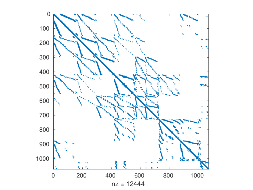
(a) HB/can_1072

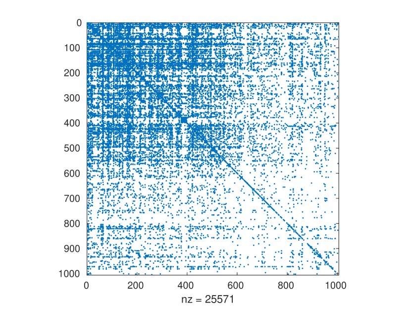
(b) SNAP/email-Eu-core

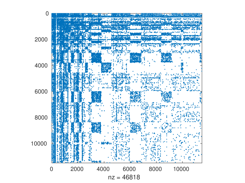
(c) SNAP/Oregon-1

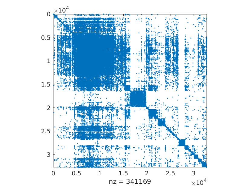
(d) SNAP/wiki-topcats

Figure 2: Spy Plots

The matrix HB/can_1072 is sparse and irreducible. The (scaled) SKK iteration is convergent. In Table 2 we compare the computing times of Algorithm 1 and 2 for different values of $\tau$. All times are in seconds and averaged over 10 runs.

Table 2: Computing times of Algorithm 1 and 2 applied to HB/can_1072 for different values of $\tau$

$\tau$	1.0e-6	1.0e-8	1.0e-10	1.0e-12	1.0e-14
Alg1	0.00296	0.0147	0.0315	0.0484	0.0657
Alg2	0.0151	0.0213	0.0213	0.0253	0.0254

As suggested at the beginning of the previous section the approach pursued by Algorithm 2 exhibits a convergent behavior under the same assumptions as the SKK iteration. Moreover, for low levels of accuracy the cost of the eigensolver is dominant whereas Algorithm 2 becomes faster than Algorithm 1 as $\tau$ decreases.

The remaining matrices (ii), (iii) and (iv) from the SNAP collections are more challenging due to the occurrence of clustered eigenvalues around 1 of $J_{T}(\mbox{\boldmath$x$})$ where $\mbox{\boldmath$x$}\in\mathcal{P}_{0}$ is a fixed point of $T$. According to [6] in order to carry out the approximation of this vector efficiently we consider perturbations of the input matrix $A$ of the form

$$\widetilde{A}=A+\gamma\mbox{\boldmath$e$}\mbox{\boldmath$e$}^{T},\quad\mbox{\boldmath$e$}=\left[1,\ldots,1\right]^{T},\quad\gamma>0,$$

for decreasing values $\gamma_{i}$, $1\leq i\leq K$, of $\gamma$. The approach resembles the customary strategy employed for solving the PageRanking problem. In the next tables 3, 4 and 5 we report the computing times of Algorithm 1 and 2. When $\gamma=\gamma_{1}$ both algorithms start with $\mbox{\boldmath$x$}=\mbox{\boldmath$e$}/n$ whereas for $i>1$ the starting vector is given by the solution computed at the previous step with $\gamma=\gamma_{i-1}$. In all experiments the tolerance was set at $\tau=1.0e-12$.

Table 3: Computing times of Algorithm 1 and 2 applied to SNAP/email-Eu-core for different values of $\gamma$

$\gamma$	1.0e-2	1.0e-4	1.0e-6	1.0e-8	1.0e-10	1.0e-12	1.0e-14
Alg1	0.004	0.009	0.04	0.34	2.84	23.24	185.54
Alg2	0.01	0.02	0.12	0.18	0.42	0.73	1.16

Table 4: Computing times of Algorithm 1 and 2 applied to SNAP/Oregon-1 for different values of $\gamma$

$\gamma$	1.0e-2	1.0e-4	1.0e-6	1.0e-8	1.0e-10	1.0e-12	1.0e-14
Alg1	0.006	0.008	0.04	0.32	2.66	21.86	174.27
Alg2	0.04	0.06	0.143	0.7	2.44	6.81	12.28

Table 5: Computing times of Algorithm 1 and 2 applied to SNAP/wiki-topcats for different values of $\gamma$

$\gamma$	1.0e-2	1.0e-4	1.0e-6	1.0e-8	1.0e-10	1.0e-12	1.0e-14
Alg1	0.02	0.02	0.18	0.69	5.96	46.26	365.56
Alg2	0.09	0.2	0.78	3.15	11.59	38.43	91.07

We observe that Algorithm 2 outperforms Algorithm 1 for sufficiently small values of $\gamma$ when the perturbed matrix is close to the original web link graph.

The second set of test problems consists of matrices which can be reduced by permutation of rows and columns to block triangular form. The reduction of the adjacency matrix of a graph in a block triangular form is related with the Dulmage-Mendelsohn decomposition [28], which is a canonical decomposition of a bipartite graph based on the notion of matching. The SKK iteration applied to block triangular matrices can not converge. Depending on the number of blocks the scalar Arnoldi method employed by the function eigs can also performs poorly. In this situation it can be recommended the use of a block Arnoldi-based eigensolver which using a set of starting vectors is able to compute multiple or clustered eigenvalues more efficiently than an unblocked routine. In our experiments we consider the function ahbeigs [29] which implements a block Arnoldi method for computing a few eigenvalues of sparse matrices. Block methods can suffer from the occurrence of complex eigenpairs. Therefore, based on the proof of Theorem 2.6 the method is applied to the symmetric matrix $G\cdot G^{T}$, $G=\operatorname{\mathcal{D}}(T\mbox{\boldmath$x$})\cdot A^{T}\cdot\operatorname{\mathcal{D}}(S\mbox{\boldmath$x$})$ which is similar to $J_{T}(\mbox{\boldmath$x$})$. The input sequence of ahbeigs is given as

OPTS.sigma=’LM’;OPTS.k=m;OPTS.V0=R0;[V,D]=ahbeigs(’afuncsym’, n, speye(n),  OPTS)

where $n$ is the size of the matrix $A$, $m$ is the number of desired eigenvalues, $R0\in\mathbb{R}^{n\times m}$ is the set of starting vectors and ’afuncsym’ denotes a function that computes the product of $G\cdot G^{T}$ by a vector where $A$ is stored in a sparse format.

For numerical testing we consider the following matrices:

1. the adjacency matrix $A_{jazz}\in\mathbb{R}^{198\times 198}$ constructed from a collaboration network between Jazz musicians. Each node is a Jazz musician and an edge denotes that two musicians have played together in a band. The data was collected in 2003 [30]. The MatLab command dmperm applied to the jazz matrix computes its Dulmage-Mendelsohn decomposition. It is found that the permuted matrix is block triangular with 11 diagonal blocks;

2. the matrix $A_{mbeause}\in\mathbb{R}^{496\times 496}$ generated by taking the absolute value of the matrix HB/mbeause from the the Harwell-Boeing collection. The original matrix is derived from an economic model which reveals several communities. This structure is maintained in the modified matrix. The MatLab command dmperm applied to $A_{mbeause}$ returns a permuted matrix with 28 diagonal blocks.

In Figure 3 we illustrate the spy plots of the input matrices and their permuted versions.

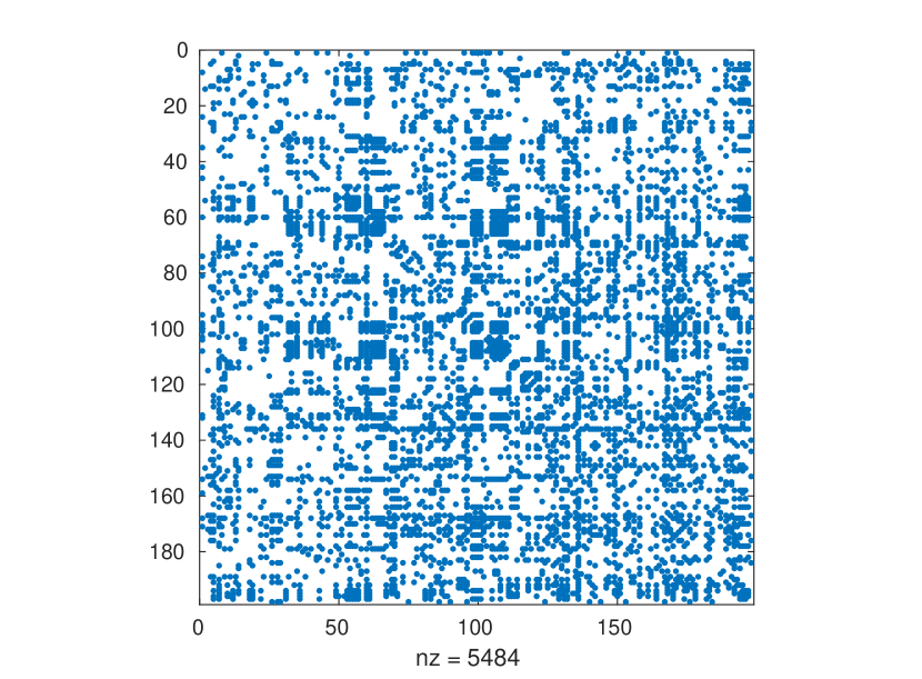
(a) $A_{jazz}$

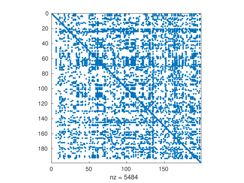
(b) Permuted $A_{jazz}$

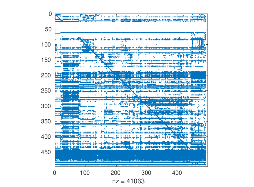
(c) $A_{mbeause}$

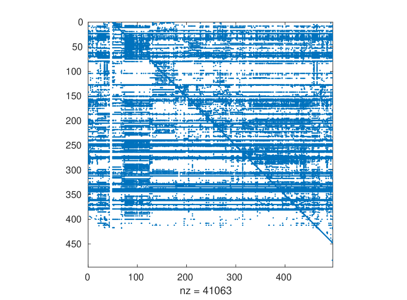
(d) Permuted $A_{mbeause}$

Figure 3: Spy Plots

In Table 6 we compare the computing times of Algorithm 1 and 2, where FDE makes use of ahbeigs, applied to the matrices $\widetilde{A}\colon=A+\gamma\mbox{\boldmath$e$}\mbox{\boldmath$e$}^{T}$ for different values of $\gamma$ and $A=A_{jazz},A_{mbeause}$. In each experiment the (block) starting vector is $X={\tt rand}(n,m)$ where $n$ is the size of $A$, $m=1$ for Algorithm 1 and $m=16,32$ for Algorithm 2 applied to $A_{jazz}$ and $A_{mbeause}$, respectively.

Table 6: Computing times of Algorithm 1 and 2 for different values of $\gamma$

	$A_{jazz}$				$A_{mbeause}$
$\gamma$	1.0e-8	1.0e-10	1.0e-12	1.0e-14	1.0e-8	1.0e-10	1.0e-12	1.0e-14
Alg1	0.06	0.18	0.68	2.87	1.87	14.43	112.26	808.26
Alg2	0.22	0.24	0.26	0.36	1.84	2.09	2.73	3.61

For these matrices the methods based on eigenvalue computations can be dramatically faster than the fixed point iteration. In particular, the modified Algorithm 2 applied to $A_{jazz}$ with $\gamma=\tau=1.0-e-12$ and $m=16$ converges in 14 iterations. In Figure 4 we show the error behavior as well as the singular values of the balanced matrix (compare with Theorem 2.3).

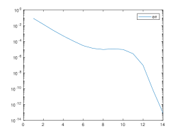
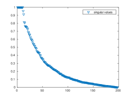
Figure 4: Error plot of modified Algorithm 2 applied to the perturbed jazz matrix and singular values of the resulting balanced matrix

It is worth stressing the accordance of the number of blocks in the permuted matrix with the size of the cluster of singular values of the balanced permuted matrix.

4 Conclusions and Future Work

In this paper we have discussed some numerical techniques for accelerating the customary SKK iteration based on certain equivalent formulations of the fixed point problem as a matrix eigenvalue problem. Variants of the power method relying upon the Arnoldi process have been proposed for the efficient solution of the matrix eigenvalue problem. There are several topics which remain to be addressed. Specifically:

1. A formal proof of the convergence for the SKK_∞ method is still missing. As suggested by Figure in this respect it might be useful to investigate the properties of the map $E\colon\mathcal{P}_{0}\rightarrow\mathcal{P}_{0}$ defined by $E(\mbox{\boldmath$v$})=\mbox{\boldmath$w$}$ where $w$ is the normalized dominant eigenvector of $J_{T}(\mbox{\boldmath$v$})$.

2. Theoretical results would be extended to nonnegative matrices under customary assumptions on their supports. Such extension can be based on the perturbative analysis introduced in [13] and Section 6.2 of [20].

3. The efficiency of the balancing schemes depends on eigenvalue (singular value) clustering properties. Numerical experiments have revealed a close connection between the clustering of singular values of the balanced adjacency matrix and the clustering of nodes (community detection) in the corresponding graph. Relations with the block triangular form (BTF) form of adjacency matrices have also appeared. The possible use of balancing schemes for detecting the block structure of adjacency matrices is an ongoing research work.

4. Finally, we plan to study the numerical behavior of block Arnoldi based methods by performing extensive numerical experiments with large sparse and data-sparse matrices. In particular following [19] we can take advantage of knowing the largest eigenvalue of the limit problem to speed up the intermediate steps.

References

- [1] Sinkhorn R. A relationship between arbitrary positive matrices and doubly stochastic matrices. Ann. Math. Statist. 1964; 35:876–879, 10.1214/aoms/1177703591. URL https://doi.org/10.1214/aoms/1177703591.
- [2] Sinkhorn R, Knopp P. Concerning nonnegative matrices and doubly stochastic matrices. Pacific J. Math. 1967; 21:343–348. URL http://projecteuclid.org/euclid.pjm/1102992505.
- [3] Sinkhorn R. Diagonal equivalence to matrices with prescribed row and column sums. Amer. Math. Monthly 1967; 74:402–405, 10.2307/2314570. URL https://doi.org/10.2307/2314570.
- [4] Parikh A. Forecasts of input-output matrices using the r.a.s. method. The Review of Economics and Statistics 1979; 61(3):477–481. URL http://www.jstor.org/stable/1926084.
- [5] Cuturi M. Sinkhorn distances: Lightspeed computation of optimal transport. Proceedings of the 26th International Conference on Neural Information Processing Systems - Volume 2, NIPS’13, Curran Associates Inc.: USA, 2013; 2292–2300. URL http://dl.acm.org/citation.cfm?id=2999792.2999868.
- [6] Knight PA. The Sinkhorn-Knopp algorithm: convergence and applications. SIAM J. Matrix Anal. Appl. 2008; 30(1):261–275, 10.1137/060659624. URL https://doi.org/10.1137/060659624.
- [7] Bozzo E, Franceschet M. A theory on power in networks. Commun. ACM Oct 2016; 59(11):75–83, 10.1145/2934665. URL http://doi.acm.org/10.1145/2934665.
- [8] Rüschendorf L. Convergence of the iterative proportional fitting procedure. Ann. Statist. 1995; 23(4):1160–1174, 10.1214/aos/1176324703. URL https://doi.org/10.1214/aos/1176324703.
- [9] Lamond B, Stewart NF. Bregman’s balancing method. Transportation Res. Part B 1981; 15(4):239–248, 10.1016/0191-2615(81)90010-2. URL https://doi.org/10.1016/0191-2615(81)90010-2.
- [10] Diamond S, Boyd S. Stochastic matrix-free equilibration. J. Optim. Theory Appl. 2017; 172(2):436–454, 10.1007/s10957-016-0990-2. URL https://doi.org/10.1007/s10957-016-0990-2.
- [11] Idel M. A review of matrix scaling and Sinkhorn’s normal form for matrices and positive maps. Technical Report, arXiv:1609.06349 2016.
- [12] Menon MV. Some spectral properties of an operator associated with a pair of nonnegative matrices. Trans. Amer. Math. Soc. 1968; 132:369–375, 10.2307/1994847. URL https://doi.org/10.2307/1994847.
- [13] Menon MV, Schneider H. The spectrum of a nonlinear operator associated with a matrix. Linear Algebra and Appl. 1969; 2:321–334.
- [14] Stewart GW. On the powers of a matrix with perturbations. Numer. Math. 2003; 96(2):363–376, 10.1007/s00211-003-0470-0. URL https://doi.org/10.1007/s00211-003-0470-0.
- [15] Knight PA, Ruiz D. A fast algorithm for matrix balancing. IMA J. Numer. Anal. 2013; 33(3):1029–1047, 10.1093/imanum/drs019. URL https://doi.org/10.1093/imanum/drs019.
- [16] Kalantari B, Khachiyan L, Shokoufandeh A. On the complexity of matrix balancing. SIAM J. Matrix Anal. Appl. 1997; 18(2):450–463, 10.1137/S0895479895289765. URL https://doi.org/10.1137/S0895479895289765.
- [17] Parlett BN, Landis TL. Methods for scaling to doubly stochastic form. Linear Algebra Appl. 1982; 48:53–79, 10.1016/0024-3795(82)90099-4. URL https://doi.org/10.1016/0024-3795(82)90099-4.
- [18] Yin J, Yin G, Ng M. On adaptively accelerated Arnoldi method for computing PageRank. Numer. Linear Algebra Appl. 2012; 19(1):73–85, 10.1002/nla.789. URL https://doi.org/10.1002/nla.789.
- [19] Golub GH, Greif C. An Arnoldi-type algorithm for computing PageRank. BIT 2006; 46(4):759–771, 10.1007/s10543-006-0091-y. URL https://doi.org/10.1007/s10543-006-0091-y.
- [20] Lemmens B, Nussbaum R. Nonlinear Perron-Frobenius theory, Cambridge Tracts in Mathematics, vol. 189. Cambridge University Press, Cambridge, 2012, 10.1017/CBO9781139026079. URL https://doi.org/10.1017/CBO9781139026079.
- [21] Brualdi RA, Parter SV, Schneider H. The diagonal equivalence of a nonnegative matrix to a stochastic matrix. J. Math. Anal. Appl. 1966; 16:31–50, 10.1016/0022-247X(66)90184-3. URL https://doi.org/10.1016/0022-247X(66)90184-3.
- [22] Lemmens B, Nussbaum R. Nonlinear Perron-Frobenius theory, Cambridge Tracts in Mathematics, vol. 189. Cambridge University Press, Cambridge, 2012, 10.1017/CBO9781139026079. URL https://doi.org/10.1017/CBO9781139026079.
- [23] Ando A, Fisher F. Near-decomposability, partition and aggregation, and the relevance of stability discussions. International Economic Review 1963; 4(1):53–67. URL http://www.jstor.org/stable/2525455.
- [24] Minc H. Nearly decomposable matrices. Linear Algebra and Appl. 1972; 5:181–187.
- [25] Simon H, Ando A. Aggregation of variables in dynamic systems. Econometrica 1961; 29(2):111–138. URL http://www.jstor.org/stable/1909285.
- [26] Courtois PJ. Decomposability. Academic Press [Harcourt Brace Jovanovich, Publishers], New York-London, 1977. Queueing and computer system applications, ACM Monograph Series.
- [27] Noóoo AN. Ranking under near decomposability. PhD Thesis, Department of Computer Engineering and Informatics, University of Patras 2016.
- [28] Ashcraft C, Liu JWH. Applications of the Dulmage-Mendelsohn decomposition and network flow to graph bisection improvement. SIAM J. Matrix Anal. Appl. 1998; 19(2):325–354, 10.1137/S0895479896308433. URL https://doi.org/10.1137/S0895479896308433.
- [29] Baglama J. Augmented block Householder Arnoldi method. Linear Algebra Appl. 2008; 429(10):2315–2334, 10.1016/j.laa.2007.12.021. URL https://doi.org/10.1016/j.laa.2007.12.021.
- [30] Gleiser P, Danon L. Community structure in jazz. Advances in Complex Systems 2003; 6(4).