Challenges of Convex Quadratic
Bi-objective Benchmark Problems

Abstract

Convex quadratic objective functions are an important base case in state-of-the-art benchmark collections for single-objective optimization on continuous domains. Although often considered rather simple, they represent the highly relevant challenges of non-separability and ill-conditioning. In the multi-objective case, quadratic benchmark problems are under-represented. In this paper we analyze the specific challenges that can be posed by quadratic functions in the bi-objective case. Our construction yields a full factorial design of 54 different problem classes. We perform experiments with well-established algorithms to demonstrate the insights that can be supported by this function class. We find huge performance differences, which can be clearly attributed to two root causes: non-separability and alignment of the Pareto set with the coordinate system.

1 Introduction

Empirical comparisons play a major role in evolutionary computation. They provide valuable insights about many practical questions that cannot be answered through theoretical analysis. Benchmarking studies can serve at least two very different purposes. The first is to reveal strengths and limitations of algorithms on previously identified challenges. To this end, benchmark problems are designed very specifically to pose one challenge, and usually only that very challenge, which allows to analyze different aspects in isolation. The second purpose is to test performance in application domains, often with functions that resemble real-world problems in a computationally tractable manner. In this paper we stick to the first paradigm.

Lists of properties making up good benchmark problems can be long and to some extent contradictory. Here we focus particularly on multi-objective (MO) optimization in continuous search spaces. For standard MO definitions and nomenclature we refer to the literature [21]. Our desiderata or design goals for benchmark problems are listed in the following:

• scalable to any search space dimension $d$ (number of variables),

• instantiable, i.e., clear how to construct (fixed or random) instances of the class of problems,

• known optimum, i.e., known Pareto front and Pareto set,

• known optimal $\mu$-distribution, i.e., optimal placement of $\mu$ points maximizing a performance indicator like dominated hypervolume,

• known challenges posed by each single objective, like non-separability, ill-conditioning, and multi-modality,

• known challenges of the multi-objective problem, like a convex or concave Pareto front,

• non-trivial and non-degenerate Pareto set.

There are good reasons to extend this list further, for example with the criteria listed in the excellent review [11]. However, in this paper we do not aim to provide a benchmark collection that covers all possible needs. We pursue two goals: we explore the utility of convex quadratic function for the construction of multi-objective benchmark problems, and doing so, we aim to cover the above list of design goals, which is somewhat tailored to convex quadratic problems.

There exist several collections of benchmark problems that are used frequently to assess properties of evolutionary multi-objective optimization algorithms. We limit ourselves to collections of generic multi-objective problems, without a particular focus. None of the existing collections fulfills all of the above goals. Here we highlight rather different examples of benchmark suites following clear design principles:

• The scalable ZDT [21] and DTLZ [6] problems are constructed around a known Pareto set and a corresponding front. At least in the bi-objective case, optimal or near-optimal $\mu$-distributions are known [1, 8]. Knowing Pareto set, Pareto front and optimal $\mu$-distribution is sufficient to assess the convergence behavior with respect to basically all convergence and spread indicators, and to define target values for algorithm comparisons as done in the bi-objective BBOB suite. There is only one instance per problem and it is unclear how to generalize them to whole classes, so that variants could be constructed. Several MO-specific challenges are known by construction, but the characteristics of the individual functions are not considered. The Pareto set is located on an edge of the feasible region, and it is hence aligned with the coordinate system, which is arguably an unrealistically simple case ([13] addresses this issue). These problems fulfill goals G1, G3, G4, and G6. Some of the shortcomings of these benchmarks sets were addressed by the walking fish group benchmarks [12], however, with a strong focus on various sub-goal of G6. Similar properties apply to the LSMOP benchmarks [4], which are largely based on DTLZ and WFG.

• The bi-objective BBOB problem suite [19] consists of 55 problems constructed through pairing of single-objective (SO) problems drawn from 10 function classes. The functions inherit scalability, variability, and known challenges from the well-known single-objective BBOB problems, however, the resulting Pareto sets and fronts are not known analytically, and it is not clear how the SO challenges translate into MO challenges. Bi-objective BBOB fulfills goals G1, G2, G5, and G7.

• The very recent work of [18] is closest to our approach. It goes into great detail in investigating theoretical properties of bi-objective functions. However, our construction of problems with a simple Pareto set is significantly more general.

We find that different construction methods result in different goals being reached. The first two goals are rather easy to cover, and so is G4 in the bi-objective case, provided that G3 is fulfilled. However, goal G3 is hard to achieve when starting from single-objective problems, which is an attractive approach since it can potentially leverage the large body of work done in the single-objective domain. Also, there is a clear tension between goals G5 and G6: while the BBOB-style construction of problems from single objectives does not yields analytical knowledge of the Pareto front, the ZDT/DTLZ-style construction does not provide much control over the objectives in isolation. In this paper we aim to resolve this conflict by providing a construction method that fulfills all of the above goals simultaneously.

2 Quadratic Bi-Objective Problems

Convex quadratic objective functions on $\mathbb{R}^{d}$ of the form $x\mapsto\frac{1}{2}x^{T}Hx+gx+c$ with positive definite Hessian matrix $H$ are of significant relevance, simply because every twice continuously differentiable function is locally approximated by its second order Taylor expansion, and under the mild regularity condition of a strictly positive definite Hessian in a (local) optimum it is of the above form.

2.1 The Single-Objective Case

For the above reason, in the single-objective case, fast convergence on a large class of functions is ensured by fast convergence on convex quadratic problems. The Covariance Matrix Adaptation (CMA) mechanism [10] found in most modern evolution strategies suits this challenge well.

Eigen-decomposition $H=UDU^{T}$ of the Hessian $H$ into an orthogonal matrix $U$ of eigen vectors and a diagonal matrix $D$ holding the (positive) eigen values is the central mathematical tool for describing, understanding and constructing this problem class. It can represent two challenges: ill-conditioning and non-separability. Ill-conditioning refers to a large conditioning number, defined as the quotient $\kappa$ of maximal and minimal eigen values of $H$ (or $D$). Separability plays a role only if the conditioning number is larger than one. A separable problem is described by $U=\mathrm{I}$, which means that there exist no cross-terms between variables, while a non-separable problem is characterized by dependencies between variables, or equivalently, by eigen vectors that are not axis-aligned. The sphere function characterized by $H=U=D=\mathrm{I}$ is the simplest quadratic problem. The ellipsoid problem features a spectrum of eigen values in some range, often set to $\kappa=10^{6}$, chosen equally spaced on a logarithmic scale. Other benchmark problems of interest are the cigar (single small eigen value, $d-1$ large eigen values) and discus (single large eigen value, $d-1$ small eigen values) functions, usually with the same $\kappa$ but different eigenvalue distribution [9]. The functions are named after the shapes of their level sets, see figure 1 for an illustration of the three-dimensional case.

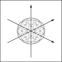
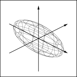
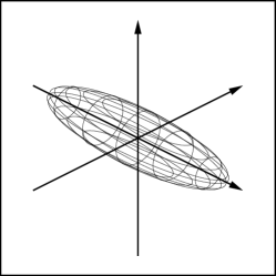
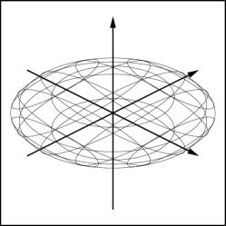
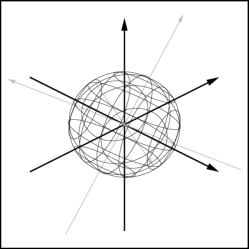
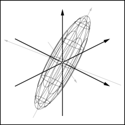
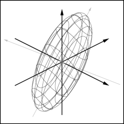
Figure 1: A single level set of the functions sphere, ellipsoid, cigar, and discus. The first row shows separable variants of the functions. In the second row the functions are rotated (the rotated axes are displayed in gray), resulting in non-separable problems in all cases except for sphere, which is rotation invariant.

Cholesky decomposition of the Hessian into $H=AA^{T}$ offers a different perspective: the matrix $A$ can be thought of as a transformation matrix between the “intrinsic” coordinate system of the quadratic function (the coordinate system in which the Hessian becomes the identity matrix) and the “extrinsic” coordinates in terms of which the problem is stated [20]. To make the Cholesky factor unique it can be chosen either as a triangular matrix with positive diagonal or as the symmetric positive definite matrix $A=U\sqrt{D}U^{T}$.

2.2 The Bi-Objective Case

In this section we investigate convex quadratic bi-objective problems in detail. There is surprisingly little literature on this topic. The probably earliest quadratic bi-objective benchmark is Schaffer’s pair of one-dimensional spheres [17]. Bi-objective BBOB [19] contains three purely quadratic functions in arbitrary dimensions, namely combinations of sphere and separable ellipsoid. The work of Augusto et al. [2] focuses on two-dimensional problems and shows how to obtain the Pareto front in the white-box case, see equation (3) below. A similar analysis is found in [16]. Here we are interested in designing benchmarks for black-box solvers, but for goals G3 to G6 an analytic understanding of the problem in the white-box sense is crucial. A set of quadratic functions with different focus was recently presented in [18].

Although convex quadratic functions are one of the simplest non-trivial MO problem classes, we demonstrate that they pose significantly richer challenges than in the single-objective case. Indeed, some of these were apparently not considered in the existing literature.

Without loss of generality (see section 3.2) we parameterize the objective functions as

$$f_{i}(x) =\frac{1}{2}(x-x_{i}^{*})^{T}H_{i}(x-x_{i}^{*})$$

$$=\frac{1}{2}(x-x_{i}^{*})^{T}A_{i}A_{i}^{T}(x-x_{i}^{*})=\frac{1}{2}\big{\|}A_{i}^{T}(x-x_{i}^{*})\big{\|}^{2}$$ (1)

$$=\frac{1}{2}(x-x_{i}^{*})^{T}U_{i}D_{i}U_{i}^{T}(x-x_{i}^{*})$$

for $i\in\{1,2\}$, where $x_{i}^{*}$ is the optimum of $f_{i}$. The Hessian matrices $H_{i}$ are symmetric and strictly positive definite. They are represented by their eigen decomposition into orthogonal $U_{i}$ and strictly positive definite diagonal $D_{i}$, or alternatively by their Cholesky factors $A_{i}$. Furthermore we define $\delta=x_{2}^{*}-x_{1}^{*}$, and in order to avoid trivial degenerate cases we assume $\delta\not=0$.

A point $x\in\mathbb{R}^{d}$ is Pareto optimal if for all $y\in\mathbb{R}^{d}$ it holds either $f_{1}(x)\leq f_{1}(y)$ or $f_{2}(x)\leq f_{2}(y)$ (assuming minimization of $f_{1}$ and $f_{1}$). For a smooth function a necessary condition is that the gradients $\nabla f_{i}(x)=H_{i}(x-x_{i}^{*})$ of the two objectives cancel out [2, 15, 18], i.e., that

$$c\cdot H_{1}(x-x_{1}^{*})+(1-c)\cdot H_{2}(x-x_{2}^{*})=0$$ (2)

for some $c\in[0,1]$. We obtain Pareto optimal solutions of the form

$$x=(cH_{1}+(1-c)H_{2})^{-1}\big{[}cH_{1}x_{1}^{*}+(1-c)H_{2}x_{2}^{*}\big{]},$$ (3)

see also [2, 18]. Hence, in a white-box setting the problem is solved analytically. In accordance with goal G3 we want this set to be of a tractable form. This is the case in particular if $\delta$ is a generalized eigenvector of the pair $(H_{1},H_{2})$, i.e., if it holds $gH_{1}\delta-(1-g)H_{2}\delta=0$ for $g\in[0,1]$. Restricted to the affine line spanned by $x_{1}^{*}$ and $x_{2}^{*}$ equation (2) is a generalized eigen value problem. By plugging the parameterization

$$x=(1-t)\cdot x_{1}^{*}+t\cdot x_{2}^{*}=x_{1}^{*}+t\delta=x_{2}^{*}-(1-t)\delta$$

for $t\in[0,1]$ into equation (2) we obtain

$$ct\cdot H_{1}\delta=(1-c)(1-t)\cdot H_{2}\delta.$$

For each $t\in[0,1]$ there exists $c\in[0,1]$ such that it holds $(1-c)(1-t)g=ct(1-g)$, so that the generalized eigen equation is fulfilled. Therefore the Pareto set is given by the line segment

$$S=\Big{\{}(1-t)\cdot x_{1}^{*}+t\cdot x_{2}^{*}\,\Big{|}\,t\in[0,1]\Big{\}}.$$

The corresponding Pareto front is convex [18]. Let $n_{1}=f_{1}(x_{2}^{*})$ and $n_{2}=f_{2}(x_{1}^{*})$ denote the components of the nadir point, then the Pareto front is the parameterized set

$$F=\left\{\left.\left(t^{2}\cdot n_{1},\left(1-t\right)^{2}\cdot n_{2}\right)\,\right|\,t\in[0,1]\right\}.$$

2.3 Non-Separability and Ill-Conditioning

As noted above, non-separability and ill-conditioning can be defined in terms of the matrices $U_{i}$ and $D_{i}$. Here we take a slightly different perspective based on the Cholesky factors $A_{i}$, which we think of as transformations between the “intrinsic” coordinates in which the quadratic problem is a sphere function and the given “extrinsic” coordinates. In the bi-objective case, three coordinate systems are involved: the extrinsic system and two intrinsic ones. The standard notion of non-separability and ill-conditioning asks how well or how badly intrinsic systems are aligned with the extrinsic one, in the terms defined above, which involve $U_{i}$ and $D_{i}$. However, we can equally well ask whether the two intrinsic coordinate systems are aligned or not. In the simplest case both objectives share the same Hessian, and in the worst case their Hessians differ significantly. In the latter case, the variations (e.g., mutations) that are most suitable for creating successful offspring may vary when moving along the Pareto front.

Based on the above considerations we define a total number of nine cases with different properties in terms of non-separability and ill-conditioning:

• All three coordinate systems are aligned, i.e., $U_{1}=U_{2}=\mathrm{I}$.

  • Both functions are (shifted) spheres: $D_{1}=D_{2}=\mathrm{I}$ and hence $H_{1}=H_{2}=\mathrm{I}$.

  • One function is a sphere, the other one is not: $D_{1}=\mathrm{I}\not=D_{2}$.

  • Both functions are ill-conditioned in the same way: $D_{1}=D_{2}\not=\mathrm{I}$.

  • Both functions are ill-conditioned in different ways: $\mathrm{I}\not=D_{1}\not=D_{2}\not=\mathrm{I}$.

• One intrinsic coordinate system is aligned with the extrinsic one, the other one is not: $U_{1}=\mathrm{I}$, $U_{2}\not=\mathrm{I}$, $D_{2}\not=\mathrm{I}$.

  • $f_{1}$ is a sphere, i.e., $D_{1}=\mathrm{I}$.

  • The Hessians are unrelated: $\mathrm{I}\not=D_{2}\not=D_{1}\not=\mathrm{I}$.

• No intrinsic coordinate system is aligned with the extrinsic one, but they are aligned with each other: $U_{1}=U_{2}\not=\mathrm{I}$ and $D_{1}\not=\mathrm{I}\not=D_{2}$.

  • For $D_{1}=D_{2}$ both problems share the same Hessian.

  • Otherwise the two functions are aligned but differently scaled.

• No pair of coordinate systems is aligned with each other:

  • $\mathrm{I}\not=U_{1}\not=U_{2}\not=\mathrm{I}$, $D_{1}\not=\mathrm{I}\not=D_{2}$.

Whenever matrices are unequal in the above list then, for the purpose of sampling instances, we assume that they are “significantly different” with high probability. For orthogonal matrices this is the case for example if $U_{1}^{T}U_{2}$ follows a uniform distribution on the set of orthogonal transformations. For diagonal matrices we demand that $D_{1}^{-1}D_{2}$ has a large conditioning number.

These classes fulfill all goals up to G6: They are scalable, we will show in the next section how to create instances, the Pareto set is a line segment in a special or general direction, the front is convex, for which the optimal $\mu$-distribution is easy to obtain numerically with the methods of [1] or [8] (and this needs to be done only once), and single-objective challenges like non-separability and ill-conditioning are exactly what defines the different problem classes. Goal G6 will be addressed in section 2.5.

It is worth pointing out that the construction is more general than rotating (essentially) separable benchmarks, as proposed in [13]. This is because we apply independent affine transformations to the two objectives, which provides great flexibility.

2.4 Alignment of the Pareto Set

The Pareto sets of all problems under consideration form line segments. It makes sense to ask whether or not the line segment is aligned with the extrinsic coordinate system. The answer depends on properties of the Hessians since we always assume that $\delta$ is a generalized eigenvector thereof. For some cases it is easy to construct aligned and non-aligned instances, while in others we need to consider additional constraints (see also section 3). At first glance, cases 2, 3 and 4 demand that $\delta$ is axis-aligned since all generalized eigen values have this property. However, even in this case we can construct non-aligned Pareto sets. For this purpose we demand that at least one generalized eigen space is at least two-dimensional. Within this subspace the vector $\delta$ can be chosen freely. The resulting vector is sparse (the number of non-zeros equals the dimension of the eigen space), but not aligned with a single axis. This can be sufficient to detect whether variation operators are able to move along a non-aligned Pareto set.

With this construction, we extend the above scheme, consisting of nine classes. For each class we consider two sub-classes, namely for axis-aligned $\delta$ and for non-aligned $\delta$. The aligned case is denoted by appending a vertical bar (ASCII pipe, "|") to the class number, and a tilted bar (ASCII slash, "/") denotes the non-aligned case. For example, 1/ is the class of problems consisting of two sphere functions with optima $x_{1}^{*}$ and $x_{2}^{*}$ in general position, while for class 7| the objectives are jointly rotated ellipsoid functions with axis-aligned Pareto set. Two-dimensional example instances of some of the problem classes are illustrated in figure 2.

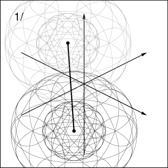
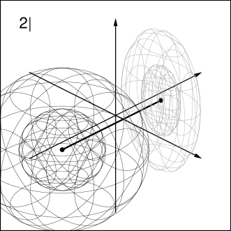
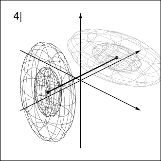
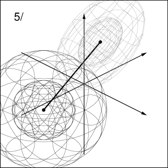
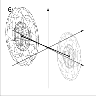
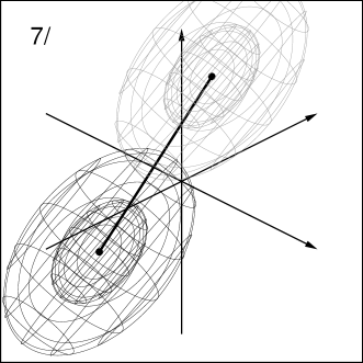
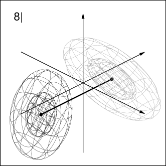
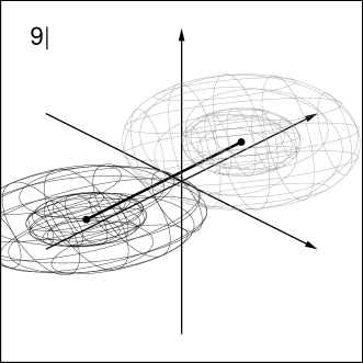
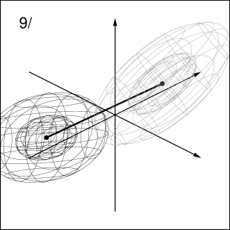
Figure 2: Level sets of the two objective functions for 9 out of the 18 quadratic problem classes, for a benign conditioning number of $\kappa=10$. The black dots are the optima of the two objectives, and the line connecting the two is the Pareto set. The problems vary in level set shapes, level set alignment with each other and/or with the coordinate system, and alignment of the Pareto front with the coordinate system.

2.5 Multi-Objective Challenges

In this section we consider challenges that are specific to multi-objective optimization. This is a wide field, and in order not to deviate too widely from quadratic function, here we only scratch the surface.

As shown in equation (1), every quadratic function $f(x)$ can be written as the sphere function $g(x)=\frac{1}{2}\|x\|^{2}$ applied to the linearly transformed point $h(x)=A^{T}(x-x^{*})$: $f(x)=g\big{(}h(x)\big{)}$. The whole power of the construction until now relies on flexibly constructed transformations $h$. Multi-objective challenges are best constructed by varying $g$.

A simple modification that does not even change the level sets of the individual objectives is to use a different power for the Euclidean norm: $g(x)=\frac{1}{2}\|x\|^{s}$. A pair of quadratic spheres ($s=2$) yields a convex front. A linear front is obtained for $s=1$, and a concave front for example with $s=1/2$ (a quarter of an ellipse) [7]. We mark these cases by appending the upper case letters C, I and J to the problem name, resembling a convex, linear, and concave shape.

Similar constructions were applied in the construction of the ZDT, DTLZ, and WFG functions. These function classes go beyond our approach in several respects, and they provide systematic construction kits. In order to limit the complexity of our construction we do not follow this well-explored road, and we limit goal G6 to the above three shapes of the Pareto front. Anyway, it is worth mentioning that it should be possible to combine our construction with other challenges by applying the 18 different classes of transformations first, followed by existing techniques, which are suitable for generating disconnected, partially flat, combined convex/concave, or otherwise interesting front shapes.

2.6 Extension to $m>2$ Objectives

It is straightforward to extend our construction to more than two objectives. However, making sure that the Pareto set is of a tractable form is a bit more challenging, since it requires pairwise compatibility of all Hessians. Also, a fully factorial design would result in a combinatorial explosion of different cases. This is not only undesirable, but also unnecessary. For example, it is probably sufficient to test cases where subsets of the objective functions use an aligned coordinate system. Instead, either all functions should either be jointly or independently rotated, or none. Also, an $m-1$ dimensional Pareto set can be fully aligned to the coordinate system or be in general position, while partial alignment is unlikely to provide additional insights. This way it is possible to stick to the 18 classes of transformations identified above.

3 Benchmark Construction

In this section we discuss how to construct instances of the benchmark problem classes. To this end we will fix a few remaining design decisions. The main problem tackled in this section is how to sample from spaces of function under a variety of different constraints defining the different problem classes.

In the following we will always assume that $\delta$ is a generalized eigenvector of $(H_{1},H_{2})$. Technically this can be achieved by setting $\delta$ first and by constructing appropriate matrices $H_{i}$, or by fixing $H_{i}$ arbitrarily and picking $\delta$ as one of the generalized eigen vectors. We will use both approaches in the following, depending on the constraints posed by the different cases.

We aim to construct all 18 classes of transformations according to the same scheme, as far as possible. We first discuss a straightforward approach that works only in the absence of constraints, and then turn to sampling procedures for constrained cases.

3.1 Sampling with and without Constraints

If an orthogonal matrix $U_{i}$ differs from the identity then we sample it from the uniform distribution on the orthogonal matrices. An easy to implement sampling procedure is to create a $d\times d$ matrix with entries sampled i.i.d. from the standard normal distribution $\mathcal{N}(0,1)$, and to apply the Gram-Schmidt orthogonalization process. For diagonal matrices that differ from the identity we apply the eigen value spectrum of the ellipsoid function $D_{ii}=\kappa^{\frac{i-1}{n-1}}$ with default value $\kappa=10^{3}$, corresponding to a non-trivial yet moderate conditioning number. However, we randomly permute the eigen values. The point $(x_{1}^{*}+x_{2}^{*})/2$ is sampled from the multivariate standard normal distribution $\mathcal{N}(0,\mathrm{I})$ under the additional constraint that no component exceeds the range $[-4.5,4.5]$. The vector $\delta$ is defined as a generalized Eigen vector of the pair $(H_{1},H_{2})$ selected uniformly at random and scaled to unit length. This uniquely determines the points $x_{i}^{*}$. The construction guarantees that the Pareto set is contained in the hypercube $[-5,5]^{d}$. The ability to provide bounds makes variation operators for bounded spaces applicable as they are used by several popular algorithms.

The above procedure is unable to produce instances of cases 2/, 3/, and 4/, which require an at least two-dimensional generalized eigen space. We therefore use the eigen values of the $(d-1)$-dimensional case and duplicate one eigen value at random. Furthermore we ensure that the duplicate eigen values are in the same position in both diagonal matrices. Then $\delta$ is non-zero only in these two coordinates (called $i$ and $j$), with $\delta_{i}=\cos(\alpha)$ and $\delta_{j}=\sin(\alpha)$ with $\alpha$ uniform on $[0,2\pi]$.

Another constraint is posed in cases 5|, 6|, 7|, 8|, 9|, which require an axis-aligned vector $\delta$ despite non-trivial orthogonal transformations being in place. In cases 5| and 6| this is achieved by modifying the random matrices before applying Gram-Schmidt orthogonalization. We fix a random index $i\in\{1,\dots,d\}$ and set the $i$-th row and column to zero, while the diagonal value is set to one. In cases 7| and 8| the same procedure is applied to both random matrices with the same index $i$. In these cases, $\delta$ is the vector consisting of $d-1$ zeros with a single one in position $i$.

Case 9| is solved differently. First all matrices are sampled as in case 9/, and $\delta$ is determined. Then a further orthogonal matrix $U$ is created based on a matrix with i.i.d. Gaussian entries, however, with the first column fixed to $\delta$. When orthogonalized, the Gram-Schmidt process starts with the first column of the matrix and hence leaves $\delta$ unchanged. After orthogonalization, $\delta$ is swapped with a random column. Finally, $U_{1}$ and $U_{2}$ are replaced with $U^{T}U_{1}$ and $U^{T}U_{2}$, and we replace $\delta$ with $U^{T}\delta$.

3.2 Reproducible Instances

Instances of the above defined problem classes can be constructed by following the sampling procedures defined above. The easiest way to define reproducible instances is to fix the seed of the random number generator used for sampling. This yields a nearly arbitrarily large number of instances at no additional cost. We use a 19937-bit Mersenne twister for this purpose.

Our sampling procedure does already produce instances that vary in terms of typical transformations of the input space like translation, rotation (as far as possible within the problem class), and permutation of variables. However, all functions are still defined on the same scale of values, and the componentwise optima have a value of zero. In order to avoid any bias in the evaluation we also vary these.

To this end we argue that strictly monotone transformations of the objective functions do not change the Pareto set [18] and the level sets of the component functions, and hence can be considered simple variants of the same problem class. We propose to apply affine linear transformations of the form $a_{i}f_{i}+b_{i}$ with $a_{i}>0$. We sample $\log_{10}(a_{i})$ and $b_{i}$ from the uniform distributions on $[0,6]$ and $[-a_{i},+a_{i}]$, respectively.

At this point our construction has the general form

$$f_{i}(x)=\frac{a_{i}}{2}\left[(x-x_{i}^{*})^{T}U_{i}D_{i}U_{i}^{T}(x-x_{i}^{*})\right]^{s/2}+b_{i}.$$

It represents a total of $9\cdot 2\cdot 3=54$ function classes. This full factorial design allows for a detailed analysis of factors impacting performance.

A problem instance is defined by the parameters $a_{i}$, $b_{i}$, $U_{i}$, $D_{i}$, $x_{i}^{*}$, and $s$. These parameters can be obtained from the sampling procedures defined above for all 18 classes of transformations with their different constraints.

4 Experiments

We have implemented our benchmark collection in C++ based on the Shark machine learning library [14]. Given a problem class name, a dimension and an instance index it creates a problem instance that can be evaluated. The code is provided in the supplementary material.

In order to exemplify the insights that can be gained just from quadratic benchmarks we run experiments with MO-CMA-ES [13] with hypervolume-based selection, SMS-EMOA [3], and NSGA-II [5]. We also tried NSGA-III, but it performed consistently worse than its predecessor, simply because the newer method is designed for many-objective problems, while we consider only $m=2$ objectives. All methods were applied with their default operators as implemented in the Shark library [14].

Let $u$ and $n$ denote utopian and nadir point, respectively. We define the reference point for the calculation of the dominated hypervolume as $\frac{11n-u}{10}$, which amounts to shifting the nadir by $10\%$ of the distance between utopian point and nadir point. This setting ensures that identifying the extreme points pays off [1], but without over-emphasizing their role. The hypervolume itself differs by many orders of magnitude, depending on the problem instance. In order to obtain a less problem dependent measure, we divide it by the area between utopian point and nadir point, which is of size $(n_{1}-u_{1})\times(n_{2}-u_{2})$. We refer to the quotient as the normalized dominated hypervolume.

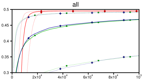
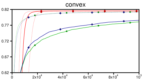
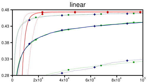
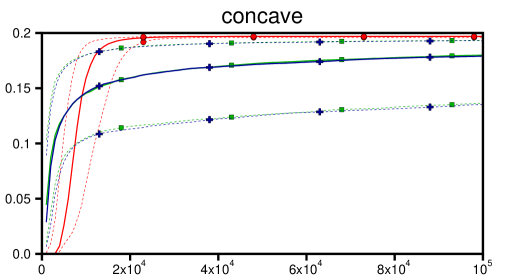
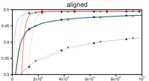
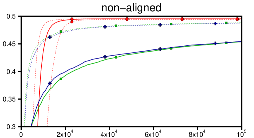
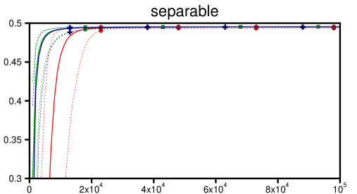
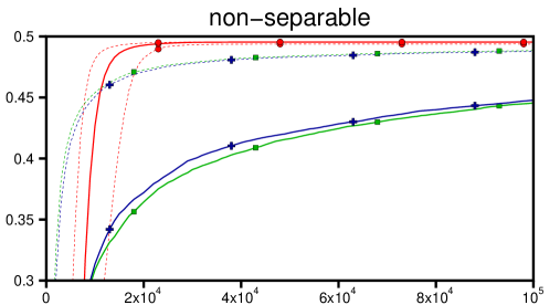
Figure 3: Average performance of MO-CMA-ES, SMS-EMOA, and NSGA-II over eight different problem groups. The plots show dominated hypervolume, averaged over problem classes and 101 instances per problem, over number of fitness evaluations. The solid curves are medians over 101 problem instances, the dashed curves are the corresponding 10% and 90% quantiles.

We ran the three above-mentioned algorithms on 101 instances of each of the 54 problem classes defined in the previous section. The search space was of dimension $d=10$, and we set the population size of all three algorithms to $\mu=20$. The bounds of the variables for SMS-EMOA and NSGA-II were set to $[-5,5]$ (containing the Pareto set), and MO-CMA-ES was initialized at the origin with an initial step size of $\sigma=3$, yielding a roughly comparable initial distribution. Each solver was given a (rather generous) budget of $100,000$ fitness evaluations.

This setup is by no means a distinguished one, and one could experiment with many parameters, in particular with the problem dimension $d$ and with the population size $\mu$. Here we refrain from an extensive experimental study, since in this work comparing different algorithm is only a side product, while our central aim is to demonstrate our class of convex quadratic multi-objective benchmarks.

4.1 Results

The evolution of the normalized dominated hypervolume is shown in figure 3 for eight selected groups of functions. Of course, depending on the research question each function can be considered individually, and it can be contrasted with other functions to demonstrate specific effects. Here we focus on groups identified already in section two, namely different shapes of the front, axis-aligned and non-aligned Pareto sets, and separable vs. non-separable problems.

4.2 Discussion

Figure 3 reveals tremendous differences in performance. Generally speaking, MO-CMA-ES excels on all problems, and its performance is nearly constant across all problems groups. This is no surprise, given its very good performance on quadratic single-objective problems, for which covariance matrix adaptation is a perfect match, as well as its invariance properties.

In contrast, the variation operators of SMS-EMOA and NSGA-II are beneficial only in an early phase, and later on for separable problems. The inability of the variation operators to model directions other than the given problem axes apparently causes a severe degradation in performance in all other cases.

In contrast, the shape of the front has a minor impact on performance (note that the achievable dominated hypervolume differs, while all plots show a range of 0.2, measured in normalized dominated hypervolume).

The question whether the Pareto set is aligned with a problem axis or not has a larger impact, and a more fine-grained analysis (analyzing plots for each single transformation, not shown for space limitations) reveals that the difference is most pronounced for cases 8| and 8/ and 9| and 9/, where none of the objective functions is aligned with the coordinate system.

An even more pronounced degradation of optimization performance for SMS-EMOA and NSGA-II is caused by rotating the coordinate system, which causes non-separability.

In summary, we can conclude that the variation operators of NSGA-II and SMS-EMOA are not well suited as soon as the Pareto set is not aligned with a coordinate axis, and as soon as the problem is non-separable. These seem to be very reasonable assumptions for black-box real-world problems. Of course, due to the very nature of convex quadratic functions, we can conclude superiority of MO-CMA-ES only for the challenges of non-separability and ill-conditioning, which are by no means the only challenges in multi-objective optimization problems.

5 Conclusion

We have constructed an expressive set of problem classes for testing bi-objective optimization algorithms from rather simple primitives, namely from convex quadratic functions. Our construction procedure addresses shortcomings of existing benchmark collections, and we hope that the 18 transformation classes will enter future benchmark construction procedures.

We discovered novel challenges that were not considered before (to the best of our knowledge), like alignment of the function with the given coordinate system (separability) vs. alignment of the objectives with each other, and the distinction between separability and the alignment of the Pareto set with the coordinate axes.

Despite the limited versatility of convex quadratic functions, our benchmark collection exhibits high discriminative power as demonstrated in the experiments, where extreme performance differences can be observed and clearly attributed to properties of the benchmarks, which are known by construction. We have not yet exploited the full potential of the construction, which also provides full knowledge of Pareto set and Pareto front. Such information is invaluable for algorithm comparison and analysis purposes.

References

- [1] A. Auger, J. Bader, D. Brockhoff, and E. Zitzler. Theory of the Hypervolume Indicator: Optimal -Distributions and the Choice of the Reference Point. In Proceedings of the tenth ACM SIGEVO workshop on Foundations of genetic algorithms, pages 87–102. ACM, 2009.
- [2] O.B. Augusto, F. Bennis, and S. Caro. Multiobjective optimization involving quadratic functions. Journal of Optimization, 2014.
- [3] N. Beume, B. Naujoks, and M. Emmerich. SMS-EMOA: Multiobjective selection based on dominated hypervolume. European Journal of Operational Research, 181(3):1653–1669, 2007.
- [4] Ran Cheng, Yaochu Jin, Markus Olhofer, and Bernhard Sendhoff. Test problems for large-scale multiobjective and many-objective optimization. IEEE Transactions on Cybernetics, 47(12):4108–4121, 2017.
- [5] K. Deb, A. Pratap, S. Agarwal, and T. Meyarivan. A fast and elitist multiobjective genetic algorithm: NSGA-II. IEEE Transactions on Evolutionary Computation, 6(2):182 – 197, 2002.
- [6] K. Deb, L. Thiele, M. Laumanns, and E. Zitzler. Scalable Multi-Objective Optimization Test Problems. In Congress on Evolutionary Computation (CEC), pages 825–830. IEEE Press, 2002.
- [7] Michael Emmerich and André Deutz. Test problems based on lamé superspheres. In International Conference on Evolutionary Multi-Criterion Optimization (EMO), pages 922–936. Springer, 2007.
- [8] T. Glasmachers. Optimized approximation sets for low-dimensional benchmark pareto fronts. In Parallel Problem Solving from Nature (PPSN). Springer, 2014.
- [9] N. Hansen, A. Auger, R. Ros, S. Finck, and P. Pošík. Comparing results of 31 algorithms from the black-box optimization benchmarking bbob-2009. In Proceedings of the 12th annual conference companion on Genetic and evolutionary computation, pages 1689–1696. ACM, 2010.
- [10] N. Hansen and A. Ostermeier. Completely derandomized self-adaptation in evolution strategies. Evolutionary Computation, 9(2):159–195, 2001.
- [11] S. Huband, P. Hingston, L. Barone, and L. While. A review of multiobjective test problems and a scalable test problem toolkit. IEEE Transactions on Evolutionary Computation, 10(5):477–506, 2006.
- [12] Simon Huband, Luigi Barone, Lyndon While, and Phil Hingston. A scalable multi-objective test problem toolkit. In International Conference on Evolutionary Multi-Criterion Optimization, pages 280–295. Springer, 2005.
- [13] C. Igel, N. Hansen, and S. Roth. Covariance matrix adaptation for multi-objective optimization. Evolutionary Computation, 15(1):1–28, 2007.
- [14] C. Igel, V. Heidrich-Meisner, and T. Glasmachers. Shark. Journal of Machine Learning Research, 9:993–996, 2008.
- [15] P. Kerschke and C. Grimme. An expedition to multimodal multi-objective optimization landscapes. In International Conference on Evolutionary Multi-Criterion Optimization, pages 329–343. Springer, 2017.
- [16] Pascal Kerschke, Hao Wang, Mike Preuss, Christian Grimme, André Deutz, Heike Trautmann, and Michael Emmerich. Search dynamics on multimodal multiobjective problems. Evolutionary computation, pages 1–33, 2018.
- [17] J.D. Schaffer. Some experiments in machine learning using vector evaluated genetic algorithms (artificial intelligence, optimization, adaptation, pattern recognition). PhD thesis, Vanderbilt University, 1984.
- [18] C. Touré, A. Auger, D. Brockhoff, and N. Hansen. On bi-objective convex-quadratic problems. In International Conference on Evolutionary Multi-Criterion Optimization, pages 3–14. Springer, 2019.
- [19] T. Tušar, D. Brockhoff, N. Hansen, and A. Auger. COCO: The bi-objective black box optimization benchmarking (bbob-biobj) test suite. Technical Report 1604.00359, arXiv.org, 2016.
- [20] D. Wierstra, T. Schaul, T. Glasmachers, Y. Sun, J. Peters, and J. Schmidhuber. Natural evolution strategies. Journal of Machine Learning Research, 15:949–980, 2014.
- [21] E. Zitzler, K. Deb, and L. Thiele. Comparison of Multiobjective Evolutionary Algorithms: Empirical Results. Evolutionary Computation, 8(2):173–195, 2000.