Bivariate modelling of precipitation and temperature using a non-homogeneous hidden Markov model

Abstract

Aiming to generate realistic synthetic times series of the bivariate process of daily mean temperature and precipitations, we introduce a non-homogeneous hidden Markov model. The non-homogeneity lies in periodic transition probabilities between the hidden states, and time-dependent emission distributions. This enables the model to account for the non-stationary behaviour of weather variables. By carefully choosing the emission distributions, it is also possible to model the dependance structure between the two variables. The model is applied to several weather stations in Europe with various climates, and we show that it is able to simulate realistic bivariate time series.

1 Introduction

Historically, the management and planning of electricity demand and generation has involved long lasting observed or synthetic temperature time series, because temperature is the main driver of electricity demand. Then the centralized generation facilities are managed to match the anticipated demand. With a growing part of less manageable renewable generation based on wind and solar, the need for the same type of meteorological information, but not restricted to temperature anymore, emerges. The necessity for the system to be robust to as many different meteorological situations as possible involves a need for large samples of consistent evolutions of many meteorological variables, such as temperature, wind speed, solar radiation and rainfall for example. Since observation or reanalysis products are all available over quite limited time periods, stochastic weather generators are valuable tools to enrich the samples. For example, stochastic generators for temperature are commonly used as part of pricing derivatives, in relation with energy prices (Campbell and Diebold (2005), Mraoua (2007), Benth and Šaltytė Benth (2011)).

Single site multivariate models have been studied for several decades. The most widely cited model for weather variables has been proposed by Richardson (Richardson, 1981) in the framework of crop development, and lots of models have then been developed on the same basis (see Wilks and Wilby (1999) for a review). These models condition the evolution of the non-precipitation variables on two states based on occurrence and nonoccurrence of rainfall. Then the simulation of the non-precipitation variables is obtained through a multivariate autoregressive process, mostly using Gaussian distributions. In some cases, the autoregressive parameters depend on weather types. Flecher et al. (2010) extend this concept by using more weather types and skew normal distributions. The weather types are identified through classifications of the rainy and non-rainy days separately for each season and the number of weather types is chosen according to the BIC criterion. Vrac et al. (2007) define a model used for precipitation downscaling based on weather types identified a priori through classifications either of the precipitation data or of exogenous atmospheric variables. However, such a priori definitions of the weather types may not be optimal to infer the stochastic properties of the variable to generate.

Hidden Markov Models (HMM) introduce the weather types as latent variables. In theses models, the states form a latent Markov chain and conditionally to the states, the observations are independent. Although simple, they are very flexible:

• the determination of the states is data driven instead of depending on arbitrarily chosen exogeneous variables,

• they allow non-parametric state-dependent distributions,

• using few parameters, they are able to model complex time dependence for the observations.

Homogeneous HMMs are generally used for multisite generation either of rainfall occurrences (Zucchini and Guttorp, 1991) or of the whole rainfall field. Kirshner (2005) proposes an overview and tests different options for the multivariate emissions, from conditional independence to complex dependence structures, going through tree structures. Ailliot et al. (2015) offers a more recent overview of the weather type based stochastic weather generators, including HMMs. Extensions to Non Homogenous HMMs are also proposed in order to introduce a diurnal cycle (Ailliot and Monbet, 2012) or to let the probability of a hidden state depend on the value of an external input variable (Hughes and Guttorp (1994), Hughes et al. (1999)).

Recently, new ways of generating meteorological variable have been studied. As an example, Peleg et al. (2017) designed a model mixing physically and stochastically based features in order to generate gridded climate variables at high spatial and temporal resolution.

Our contribution

In this paper, we introduce a non homogeneous HMM for the single site generation of temperature and rainfall at different locations in Europe presenting different climatic conditions. The model is here designed for a single site generation, because electricity load and generation balance is more and more studied at a very local scale in relation to the decentralization of electricity generation based on renewables. Furthermore, global balance is generally studied on the basis of geographical (possibly weighted) averages of the demand and generation respectively. The proposed HMM is non homogeneous because the seasonality is introduced in the transition matrix between the hidden states, as well as in the state-dependent distributions. Most of stochastic weather generators in the literature elude the problem of the non-stationarity of weather variables by defining a different model for each season or month independently, assuming local stationarity inside each block. For example, Lennartsson et al. (2008) consider blocks of lengths one, two or three months. This approach has several drawbacks:

• the local stationarity assumption may be difficult to check,

• the data used to fit each model is obtained as a concatenation of data that do not belong to the same year. This is a problem if our data exhibits a strong time dependence,

• a stochastic weather generator should be able to simulate long times series using only one model.

Our model, in contrast, allows the generation of synthetic climate variables, without splitting the data, and without any pre-processing. Furthermore, the generation of temperature implies handling the warming trend. Whereas Flecher et al. (2010) proposed a standardization of the temperature and radiation fields beforehand, the choice has been made here to explicitly introduce a trend in the temperature generation.

One of the main issues when dealing with multivariate modeling is being able to capture the possibly complex dependence structure between the variables. We introduced the state-dependent distributions of our HMM as mixtures of tensor products (see equation (4)). This allows us, provided that the number of components in the mixture is large enough and that the marginals are well chosen, to approximate any state-dependent bivariate distribution for temperature and precipitation, without any a-priori on their dependence structure. Besides, it makes it easy to generalize the model to a larger number of variables without changing its global definition.

Although they are not detailed in this paper, we studied the theoretical properties of our model and gave theoretical guarantees for the convergence of the maximum likelihood estimator (see Section 2).

Outline

A general description of our non homogeneous HMM is given in Section 2, as well as a reminder of the existing theoretical results linked to our model. Section 3 deals with the application of the model to precipitation and temperature observations. In this section, we present the data used, then we describe more precisely the modeling framework by giving the parametrization of our model that is specific to this application, and we discuss the results for the different locations. We finally go to the main conclusions and perspectives in the last section.

2 Model

In this section, we describe the mathematical framework in which we developed our model. We first give a general definition of non-homogeneous hidden Markov models, before addressing the topic of theoretical results regarding these models. The full details of the parametrization of our model are given in section 3.2, along with its application to climate data.

2.1 General formulation

Let us first recall the definition of a finite state space hidden Markov model (HMM). Let $K$ be a positive integer and $\mathsf{X}=\{1,\dots,K\}$. Let $\mathsf{Y}$ be a Polish space equiped with its Borel $\sigma$-algebra $\mathcal{Y}$. A (non-homogeneous) hidden Markov model with state space $\mathsf{X}$ and observation space $\mathsf{Y}$ is a $\mathsf{X}\times\mathsf{Y}$-valued stochastic process $(X_{t},Y_{t})_{t\geq 1}$ defined on a probability space $(\Omega,\mathcal{A},\mathbb{P})$ such that

• $(X_{t})_{t\geq 1}$ is a Markov chain with state space $\mathsf{X}$.

• For all $t\geq 1$, the distribution of $Y_{t}$ given $(X_{s})_{s\geq 1}$ only depends on $t$ and $X_{t}$, and conditional on $(X_{s})_{s\geq 1}$, the $(Y_{t})_{t\geq 1}$ are independent. Figure 1 summarizes this dynamic.

Figure 1: The dynamic of a hidden Markov model

The key point here is that, from a statistical point of view, we do not observe the state sequence $(X_{t})_{t\geq 1}$ but only $(Y_{t})_{1\leq t\leq n}$. Hence the $X_{t}$ are called the hidden states. The law of the Markov chain $(X_{t})_{t\geq 1}$ is determined by its initial distribution $\pi$ such that, for $k\in\mathsf{X}$, $\pi_{k}=\mathbb{P}(X_{1}=k)$, and its transition matrices $(Q(t))_{t\geq 1}$ defined, for $i,j\in\mathsf{X}$ and $t\geq 1$, by $Q(t)_{ij}=\mathbb{P}(X_{t+1}=j\mid X_{t}=i)$. The conditional distributions of $Y_{t}$ given $X_{t}$ are called the emission distribution. For $t\geq 1$ and $k\in\mathsf{X}$, we shall denote by $\nu_{k}(t)$ the distribution of $Y_{t}$ given $X_{t}=k$. Formally, $Y_{t}\mid\{X_{t}=k\}\sim\nu_{k}(t)$. We assume that for any $t\geq 1$ and $k\in\mathsf{X}$, $\nu_{k}(t)$ is absolutely continuous with respect to some dominating measure $\mu$ defined on $\mathcal{Y}$ and we denote by $f_{k,t}:\mathsf{Y}\longrightarrow\mathbb{R}_{+}$ the corresponding density, which will be refered to as the emission density. When the transition matrices and emission distributions are constant over time, the corresponding model is sometimes called homogeneous hidden Markov model, or just hidden Markov model when there is no ambiguity.

Parametric framework

Assume that the transition matrices and the emission distributions depend on a parameter $\theta\in\Theta$, where $\Theta$ is a compact subset of $\mathbb{R}^{q}$, for some $q\geq 1$. We now precise the way they depend on $\theta$.

• The function $t\mapsto Q(t)$ belongs to a known parametric family indexed by an unknown parameter $\beta$ to be estimated.

• For any $t\geq 1$, the emission distributions $\nu_{k}(t)$ belong to a known (not depending on $t$) parametric family (e.g. gaussian) indexed by a parameter $\theta^{Y}(t)$. In addition, we assume that the function $t\mapsto\theta^{Y}(t)$ itself belongs to a known parametric family (e.g. affine functions), with parameter $\delta$.

• Thus we can write $\theta=(\beta,\delta)$. We will denote by $Q^{\theta}(t)$ the transition matrix at time $t$ when the parameter is $\theta$ and, for $1\leq k\leq K$, $f_{k,t}^{\theta}$ the $k$-th emission density at time $t$ when the parameter is $\theta$.

Note that we consider that the number of states $K$ is known, although this is not the case in practice. We discuss this issue in section 3.3. In this framework we proceed to the estimation of the parameters using maximum likelihood inference. Having observed $(Y_{1},\dots,Y_{n})$, the likelihood of the model when the parameter is $\theta$ and the initial distribution is $\pi$ is given by

$$p^{\theta,\pi}(Y_{1},\dots,Y_{n})=\sum_{x_{1},\dots,x_{n}}\pi_{x_{1}}Q^{\theta}(1)_{x_{1}x_{2}}f^{\theta}_{x_{1},1}(Y_{1})Q^{\theta}(2)_{x_{2}x_{3}}f^{\theta}_{x_{2},2}(Y_{2})\dots Q^{\theta}(n-1)_{x_{n-1}x_{n}}f^{\theta}_{x_{n},n}(Y_{n}).$$

Then we define the maximum likelihood estimator (MLE):

$$\hat{\theta}_{\pi,n}=\operatorname*{arg\,max}_{\theta\in\Theta}p^{\theta,\pi}(Y_{1},\dots,Y_{n}).$$

The practical computation of the MLE can be performed using the well-known Expectation Maximization (EM) algorithm. See section 3.3 for the details of this algorithm in our framework.

Theoretical guarantees

The statistical properties of hidden Markov models have been studied extensively since the 1960’s. However, general identifiability conditions have only been proved recently. Following Allman et al. (2009), the authors of Gassiat et al. (2016) proved that stationary non parametric HMM are identifiable from the law of three consecutive observations (up to permutation of the states), provided that the emission distribution are linearly independent and that the transition matrix has full rank. Alexandrovich et al. (2016) prove a similar result with slightly weaker assumptions. The properties of the maximum likelihood estimator in homogeneous HMM are now well-known. Its strong consistency has first been established by Baum and Petrie (1966) in the case where both the state space and the observation space are finite. This result has been generalized to continuous observation spaces by Leroux (1992). See also Douc et al. (2011) and references therein. The literature is less abundant when it comes to non-homogeneous hidden Markov models. In Ailliot and Pene (2015) and Pouzo et al. (2016), the authors consider models where the observation distribution depends not only on the current state, but also on previous observations, and where the transition matrices depend on the previous observations. They prove the consistency of the maximum likelihood estimator in this framework. More recently, Diehn et al. (2018) study the case of non-homogeneous hidden Markov models that can be asymptotically approximated by an homogeneous one. They introduce a quasi-maximum likelihood estimator and prove its consistency. None of the previously stated results apply to the model we introduce in this paper. In Touron (2018) however, the author obtains the consistency of the maximum likelihood estimator in HMM with periodic transition matrices and emission distributions, which applies to our model in the special case where the temperature trends are zero, or to the precipitation process alone. There is also an on-going work about HMM with trends.

3 Application to precipitation and temperature

3.1 Data

Description of the data

We used data from the European Climate Assessment and Datasets (ECA&D) project. Six weather stations were considered: Helsinki (Finland), Dresden (Germany), Verona (Italy), Huelva (Spain), Clermont-Ferrand (France) and Snåsa (Norway). For each station, the data consists of mean daily temperature and daily precipitation from 1954/01/01 to 2014/12/31. Figure 2 presents the locations of the weather stations, whereas Figure 3 shows that the distribution of temperature in the 6 stations differ in many ways: mean, variance, range, skewness, seasonal behaviour…

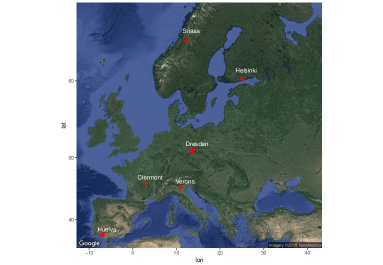
Figure 2: Stations locations

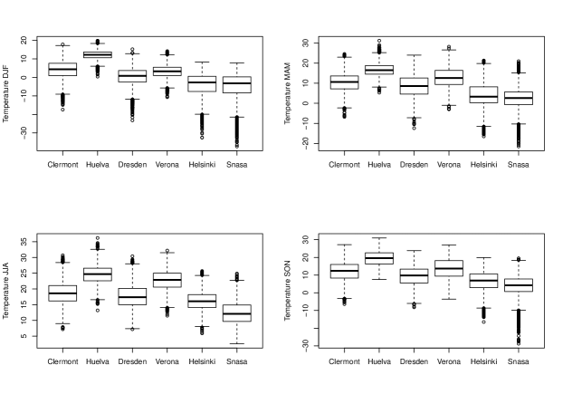
Figure 3: Boxplots of the temperature at the different locations for each season

Table 1 presents some basic statistics concerning precipitations at the 6 stations under study. Mean yearly precipitations range from 501.5 mm in Huelva (Spain) to 964.2 mm in Snåsa (Norway), where the precipitation frequency is $0.62$ compared to only $0.19$ in Huelva. Also, the maximum observed daily precipitation in Snåsa is 65.9 mm, compared to 198 mm in Verona. The mean value of (non-zero) daily precipitations ranges from 3.4 mm in Helsinki to 7.3 mm in Huelva.

	Clermont	Huelva	Dresden	Verona	Helsinki	Snasa
Mean yearly precipitation (mm)	584.2	501.5	665.3	803.3	638.9	964.2
Max. observed precipitation (mm)	75.3	160.0	158.0	198.0	79.3	65.9
Precipitation frequency	0.40	0.19	0.49	0.34	0.51	0.62
Mean positive precipitation (mm)	4.0	7.3	3.7	6.5	3.4	4.2

Table 1: Basic statistics for precipitation

We chose on purpose weather stations where climate strongly differs in order to test the robustness of our model when applied to different climates.

Seasonalities and trends

When observed at a daily time step temperature and precipitation times series are not stationary, in that their distribution varies through time. Temperature obviously exhibits a seasonal cycle, as shown on the left panel of Figure 4. The right panel of Figure 4 shows the seasonality of the variance of temperature, which is rather flat in the two stations of Southern Europe (Verona and Huelva). We also notice that these stations have the lowest variances. On the opposite, the variance of temperature displays a very clear seasonality in the stations of Northern Europe (Snåsa and Helsinki), the variability being much higher in the winter months.

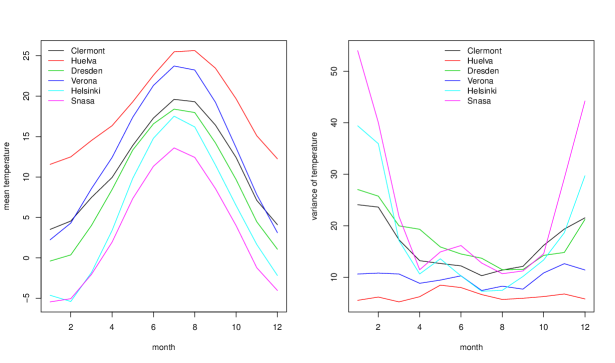
Figure 4: Monthly mean and variance of temperature

The non-stationarity of temperature is also caused by the existence of a trend, corresponding to global warming. The black lines in Figure 5 are the yearly mean temperature for each site. All sites except Huelva seem to exhibit an increasing trend. However, the shape and the slope of this trend differ among the different sites. For stations like Helsinki or Dresden it seems reasonable to consider a linear trend over the whole observed period, whereas Verona or Clermont exhibit a change point in the warming rate. Thus the modeling of the trend should be site-specific. Figure 5 suggests that a simple parametric form for the trends could be linear or piecewise linear with two pieces. Then for each site, two questions arise:

• is there a breaking point (i.e. a change in the slope of the trend)?

• if yes, where is it?

To answer these questions, we can use the yearly mean temperatures $(\bar{Y}_{a})_{a\in\{1954,\dots,2014\}}$. The linear regression is then given by

$$(\hat{\alpha}^{LM},\hat{\beta}^{LM})=\operatorname*{arg\,min}_{\alpha,\beta\in\mathbb{R}}\sum_{a=1954}^{2014}(\bar{Y}_{a}-\alpha a-\beta)^{2}$$

In a piecewise linear model, the optimal breaking point can be found by computing

$$\hat{\tau}=\operatorname*{arg\,min}_{1954\leq\tau\leq 2014}\min_{\alpha,\beta,\gamma\in\mathbb{R}}\sum_{a=1954}^{2014}(\bar{Y}_{a}-\alpha a-\beta-\gamma(a-\tau)\mathbf{1}_{t>\tau})^{2}.$$

Then the corresponding piecewise linear regression is given by

$$(\hat{\alpha}^{PLM},\hat{\beta}^{PLM},\hat{\gamma}^{PLM})=\operatorname*{arg\,min}_{\alpha,\beta,\gamma\in\mathbb{R}}\sum_{a=1954}^{2014}(\bar{Y}_{a}-\alpha a-\beta-\gamma(a-\hat{\tau})\mathbf{1}_{t>\hat{\tau}})^{2}.$$

In order to test for the significance of the breaking point, we perform a likelihood ratio test: we compute the test statistic

$$\Lambda=2\left(\log\mathcal{L}(\hat{\alpha}^{PLM},\hat{\beta}^{PLM},\hat{\gamma}^{PLM})-\log\mathcal{L}(\hat{\alpha}^{LM},\hat{\beta}^{LM})\right),$$

with $\mathcal{L}$ the likelihood function, where we considered gaussian residuals (this assumption was tested with a Kolmogorov-Smirnov test). Then $\Lambda$ is compared to a quantile of the $\chi^{2}$ distribution with one degree of freedom.

Station	Test result	p-value	$\tau$
Helsinki	PL	$0.049$	1980
Dresden	L	$0.16$	-
Verona	PL	$3.10^{-6}$	1987
Huelva	PL	$0.026$	1961
Clermont	PL	$0.012$	1978
Snåsa	PL	$0.047$	1980

Table 2: Test of the parametric form of the trends

Table 2 gives the results of this procedure for the six sites. In the ”test result” column, PL means that the test rejected the linear model at the risk level $0.05$ (which means that the trend is piecewise linear), and $L$ means that the test did not reject the linear model. The last column $\tau$ is the year of the change in the slope of the trend, when there is such a change. Thus, the test rejects the simple linear trend for all sites but Dresden. For piecewise linear trends, the breaking point is in the decade 1978-1987, which is consistent with climatology, except for the site of Huelva (1961), surprisingly. The optimal trends are depicted in Figure 5. We see that as far as Huelva is concerned, despite the result of the test, the piecewise linear trend cannot be considered significant. First, the change point in 1961 is not consistant with climatology, as it would correspond to a warming stopping in 1961. Then, we see that the procedure described above was misleaded by the unusually cold year 1956. For these reasons, we choose a simple linear trend for this station.

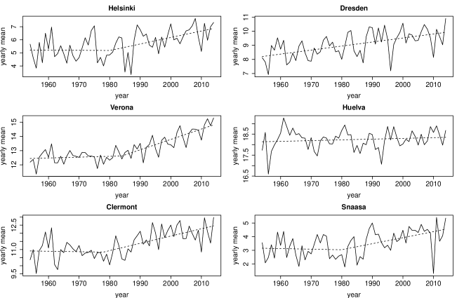
Figure 5: Yearly means of temperature (black) and associated optimal trends (blue)

Furthermore, climate change does not affect summer and winter the same way. For each location, we computed the mean temperature of summer months (June, July, August) and we centered it to remove the shift between the stations. We then applied a rolling mean with a window width of 15 years in order to smooth the effect of interannual variability. Thus the value corresponding to the year 1968 is the mean over the period 1954-1968. We performed the same operation considering winter months (December, January, February). The results can be seen in Figure 6. In summer, all the stations show an increasing trend. However, the shape of the trend may differ according to the stations. Also, the amplitude of the warming is higher in Verona ($2.5^{\circ}$C) than in Helsinki and Snåsa (about $1^{\circ}$C). In winter, the amplitude of the warming is higher in Northern Europe (Helsinki, Snåsa) than in the South (Verona, Huelva). We actually do not notice any warming in Huelva. Our model will deal with this phenomenon using seasonal transition probabilities between the states, and state-dependent trends (see Section 3.2)

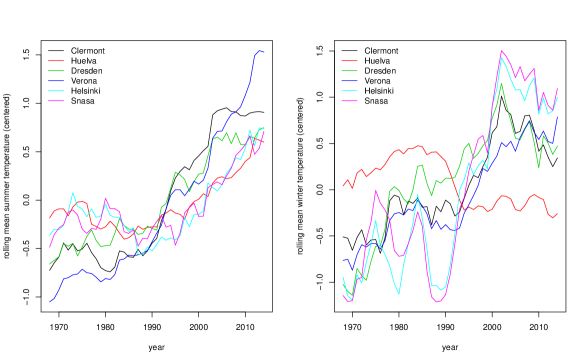
Figure 6: Temperature trend in summer (left) and winter (right)

As for precipitation, both the occurrence process (frequency of precipitation) and the intensity process have a seasonal behaviour, as shown in Figure 7. The left panel displays the frequency of precipitation, month by month, for each station. Here again, we observe that the shape as well as the amplitude of this seasonality depend on the location. In Helsinki for example, the frequency of precipitation is at its lowest in spring and at its highest in winter. It’s the opposite in Verona. The station of Huelva becomes very dry in summer and its maximum precipitation frequency is reached in January (only 0.3). The right panel in Figure 7 displays the mean value of non-zero precipitation, month by month, for every site. Observe that this quantity exhibits a strong seasonal behaviour (except in Snåsa) that is different from the one of the occurrence process. Once again, this phenomenon requires some modeling effort that we describe in Section 3.2.

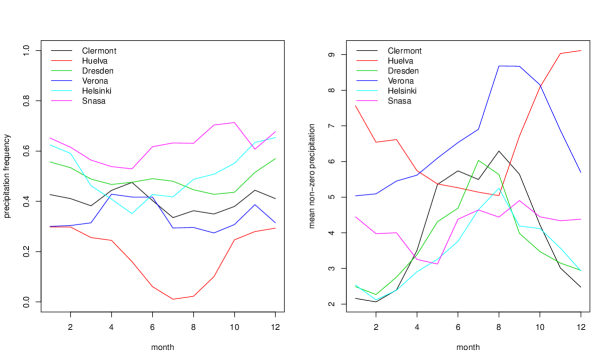
Figure 7: Seasonality of precipitation

The existence of a trend in the yearly precipitation amounts can be caused either by a trend in the occurrence process (precipitations become more rare or more frequent) or in this intensity process (the mean value of positive precipitations changes). A slight decrease of the frequency of winter precipitations can be observed in Clermont, whereas the increasing trend in winter in Snåsa is mostly the result of an increasing precipitation intensity (not shown). As these trends are light and concern only two stations, we chose not to include them in the model, which does not degrade the results.

Finally, we highlight the fact that there is also a seasonality in the dependence structure between temperature and precipitation. To see this, we can plot the monthly correlations between these two variables, as in Figure 8. All stations but Clermont share a similar shape for this curve, with a negative minimum of correlation in summer, and a positive maximum in winter. This reflects the fact the precipitations mostly occur when the temperature is moderate rather than extreme.

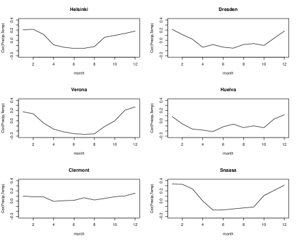
Figure 8: Monthly correlations between temperature and precipitations

3.2 Specification of the model

In section 2.1, we gave a very general description of our model. In this section, we get more into details as we give the specific forms of the transition structure and the emission distributions. As we want to model simultaneously precipitations and temperature, the observation space is $\mathsf{Y}=\mathbb{R}_{+}\times\mathbb{R}$ and $Y_{t}=\left(Y_{t}^{(1)},Y_{t}^{(2)}\right)$. The superscript $(1)$ refers to precipitation and $(2)$ refers to temperature.

Transition probabilities

The transition matrix at time $t$ in our model is given by

$$Q(t)_{ij} =\frac{\exp(P_{ij}(t))}{1+\sum_{l=1}^{K-1}\exp(P_{il}(t))},1\leq j\leq K-1,\quad 1\leq i\leq K$$ (1)

$$Q(t)_{iK} =\frac{1}{1+\sum_{l=1}^{K-1}\exp(P_{il}(t))},1\leq i\leq K.$$ (2)

This is indeed a stochastic matrix, as for all $1\leq i\leq K$, $\sum_{j=1}^{K}Q(t)_{ij}=1$ and $Q(t)_{ij}>0$. For $1\leq i\leq K$ and $1\leq j\leq K-1$, $P_{ij}$ is a trigonometric polynomial with (known) degree $d$ and period $T$. More precisely,

$$P_{ij}(t)=\beta_{ij0}+\sum_{l=1}^{d}\left(\beta_{ij,(2l-1)}\cos\left(\frac{2\pi}{T}lt\right)+\beta_{ij,2l}\sin\left(\frac{2\pi}{T}lt\right)\right)$$ (3)

Hence the transition probabilities of the hidden Markov chain are periodic functions of time. Therefore, the relative frequencies of the states will vary through time in a periodic manner. This allows the model to reproduce some of the seasonal behaviours of climate variables.

Emission distributions

In order to allow for flexibility, we choose mixtures as emission distributions. More precisely, the conditional distribution of $Y_{t}$ given $X_{t}=k$ is

$$\nu_{k}(t)=\sum_{m=1}^{M}p_{km}\nu^{(1)}_{k,m}(t)\otimes\nu^{(2)}_{k,m}(t)$$ (4)

The $p_{km}$ are the weights of the mixture, satisfying $p_{km}\geq 0$ and $\sum_{m=1}^{M}p_{km}=1$. The component corresponding to precipitations is defined by

$$\nu_{km,t}^{(1)}=\begin{cases}\delta_{0}&,1\leq m\leq M_{1}\\ \mathcal{E}\left(\frac{\lambda_{km}}{1+\sigma_{k}(t)}\right)&,M_{1}+1\leq m\leq M\end{cases},$$ (5)

where $\delta_{0}$ denotes the Dirac mass at $0$, the $\lambda_{km}$ are positive parameters depending on both the state $k$ and the population $m$ in the mixture, and $\sigma_{k}(\cdot)$ is a state-dependent trigonometric polynomial, modeling the seasonal variations of the intensity of precipitations. Thus the marginal distribution of precipitations in state $k$ at time $t$ is a mixture of a Dirac mass with weight

$$p_{k0}:=\sum_{m=1}^{M_{1}}p_{km}$$

and exponential distributions with parameters $\frac{\lambda_{km}}{1+\sigma_{k}(t)}$ and weights $(p_{km})_{M_{1}+1\leq m\leq M}$. When $p_{k0}$ is close to $1$, the state $k$ is considered as dry whereas it is considered as wet when $p_{k0}$ is close to $0$. As the frequency of a given state varies across the year thanks to the seasonal transition probabilities, this will allow the model to capture the seasonal behaviour of the frequency of precipitations.

Regarding temperature,

$$\nu_{km,t}^{(2)}=\mathcal{N}\left(T_{k}(t)+S_{k}(t)+\mu_{km},\sigma^{2}_{km}\right),$$ (6)

so that the marginal distribution of temperature in state $k$ at time $t$ is a mixture of gaussian distributions, with variances $\sigma^{2}_{km}$.

• $\mu_{km}$ is a mean parameter that depends on both the state $k$ and the component $m$.

• $T_{k}(\cdot)$ is a function corresponding to the temperature trend in state $k$. As shown in Section 3.1, the parametric form of the trends depends on the sites. We follow the conclusions of Section 3.1 and we choose linear trends for Huelva and Dresden, and piecewise linear trends (with site-specific change points) for the other stations.

• $S_{k}(\cdot)$ is a trigonometric polynomial with degree $d$ corresponding to the seasonal cycle of temperature in state $k$.

Note that we allow both the trend and the seasonality of temperature to depend on the hidden state, hence the subscript $k$. Equation (4) shows that in each state and each component of the mixture, precipitations and temperature are independent, but of course they are not globally independent. The choices of $K$, $M$, $M_{1}$ and $d$ are discussed in the next section.

3.3 Inference of the parameters

The EM algorithm

The computation of the maximum likelihood estimator is done using the EM algorithm (Dempster et al., 1977), which is a generic approach to perform maximum likelihood inference in latent variables models. The details of the algorithm in our particular framework can be found in Touron (2018). Recall that the EM algorithm does not guarantee to find the global maximum of the likelihood function but only a local maximum, depending on its initial point. To overcome this drawback, we launch the algorithm multiple times, using randomly chosen initial points. See also Biernacki et al. (2003) where the authors compare several initialization procedures for the EM algorithm.

Model selection

Our model requires to specify several hyper-parameters:

• $K$ the number of hidden states,

• $d$ the degree of the trigonometric polynomials, which sets the complexity of the seasonality,

• $M$ and $M_{1}$ which correspond to the complexity of the emission distributions.

As the dimensionality of the parameter $\theta$ is a quadratic function of $K$ and a linear function of both $d$ and $M$, the larger these hyper-parameters, the more complex the model is and the better we capture the statistical properties of the data. However, we cannot use too large hyper-parameters, for the following reasons:

• We may overfit the data.

• The M step of the EM algorithm requires to solve an optimization problem. As its solution admits no closed form, this is done using a numerical optimization algorithm, which can be difficult and time-consuming if the number of parameters is too large.

• The likelihood function of models with a large number of parameters may have many sub-optimal local maxima.

• A large number of hidden states leads to a loss of interpretability of the states, which may be a problem for some practitionners.

Therefore, the complexity of the model, especially the number of hidden states, must be chosen carefully. To do so, a standard approach is to use information criteria such as Akaike Information Criterion (AIC), Integrated Completed Likelihood (ICL, see Biernacki et al. (2000)) or Bayesian Information Criterion (BIC, see Schwarz et al. (1978)). The latter is very popular in applications of HMM, although not justified in theory. The idea of AIC and BIC is to penalize the models with a large number of parameters, in order to realize a trade-off between goodness-of-fit and complexity. If we have to choose a model among a collection $\mathcal{M}$, we minimize over $m\in\mathcal{M}$ the criterion $-\mathcal{L}(\hat{\theta}_{m})+\mathrm{pen}(m)$, where $\mathcal{L}(\hat{\theta}_{m})$ is the maximum likelihood in the model $m$, and $\mathrm{pen}(m)$ is the penalty associated to the model $m$. For example, in the case of BIC, $\mathrm{pen}(m)=-\frac{p(m)}{2}\log(n)$ where $p(m)$ is the number of parameters of the model $m$ and $n$ is the number of observations. Another approach is cross-validated likelihood (Celeux and Durand, 2008), even though it is computationally intensive. In Lehéricy (to appear), the author introduces a penalized least square estimator for the order of a nonparametric HMM and proves its consistency. However, when dealing with real world data, other considerations should be taken into account, such as interpretability of the states, computing time, or the ability of the model to reproduce some behaviour of the data, as explained in Bellone et al. (2000). Indeed, according to Pohle et al. (2017), the popular AIC (Akaike Information Criterion) and BIC, as well as other penalized criteria, tend to overestimate the number of states as soon as the data generating process differs from a HMM (e.g. the presence of a conditional dependence), which is often the case in practice. Hence it is advised to use such a criterion as a guide, without following it blindly. Keeping in mind these considerations, we chose to use the BIC criterion to select the number of states, which is by far the most important hyper-parameter because the number of parameters of the model is quadratic in $K$. We found $K=6$ or $K=7$ (depending on the stations) to be good choices. We used our previous experience on univariate models to select $d=2$, $M=4$ and $M_{1}=2$.

3.4 Results

3.4.1 Estimated parameters

As we use a hidden Markov model, we do not need to define the states a priori, thus we do not need to give them an interpretation before estimating the parameters (e.g. wet or dry state). The determination of the states is data driven and this is one of the perks of HMM. Besides, as our purpose is to produce realistic time series of weather variables, we only need to investigate on the simulations produced by the model, not its parameters. However, it is interesting to take a look at the estimated parameters themselves, thus interpreting the states a posteriori. Indeed, interpretability of the states gives credit to the model as it provides a first indication of whether or not it manages to capture some specific meteorological behaviours. We will not provide all the estimated parameters for all of the six stations. Rather, we will give some examples to shed light on the way the different parameters of our model can be physically interpreted. More precisely, the following elements are interesting to look at:

• Transitions (see Equations (1) to (3)):

  • transition matrices, specifically the functions $t\mapsto\hat{Q}_{ij}(t)$ for each pair $(i,j)\in\{1,\dots,K\}^{2}$ and $1\leq t\leq T$. The estimated transition probabilities for the station of Verona are depicted in Figure 9. This provides information on the stability of the states. For example, State $1$ is rather stable in summer, (the probability of remaining in that state is approximately $0.8$), whereas it is much less stable in winter. On the opposite, State $6$ is unstable in summer and more stable in winter.

  • the relative frequencies of the states, i.e. the probabilities $\mathbb{P}^{\hat{\theta}}(X_{t}=k)$ for $1\leq k\leq K$, $1\leq t\leq T$. These quantities can be directly obtained through the transition matrices. We represented them for the station of Verona in Figure 10. We see that they vary throughout the year, the most frequent states in summer being $1$ and $4$, whereas it is State $3$ in winter.

  

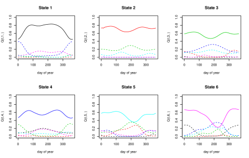
  Figure 9: Estimated transition probabilities, Verona. Each panel corresponds to a row of the transition matrices. The solid lines represent the diagonal coefficients, i.e. the functions $\hat{Q}_{ii}(\cdot)$ whereas the dashed lines represent the other coefficients. Each color corresponds to a different state.

  

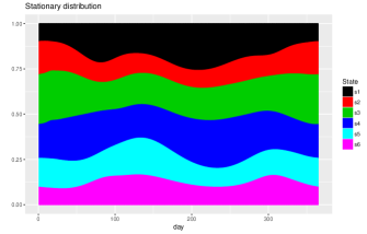
  Figure 10: Estimated relative frequencies of the states, Verona.

• Temperature parameters (see Equation (6)):

  • the trends $\hat{T}_{k}(\cdot)$ for $1\leq k\leq K$. Recall that the trends are modeled as linear for the sites of Huelva and Dresden, and piecewise linear for the others (with site-dependent breaking points) and that we estimate a different trend for each state. The results for the six stations are presented in Figure 11 and reflect an increase in mean temperature ranging from $0.6^{\circ}$C in Huelva to $\simeq 2^{\circ}$C (depending on the state) in Verona.

  • the state-dependent seasonalities $\hat{S}_{k}(\cdot)$, corresponding to the yearly cycle of temperature (see Figure 12).

  • the random noise, i.e. the centered gaussian mixture that remains, in each state, when we removed the state-dependent trend and the state-dependent seasonal component. Recall that we chose $M=4$, so that there are $4$ components in each gaussian mixture. We can see in Figure 13 some peaks in the probability density functions (especially in Dresden). These are caused by estimators $\hat{\sigma}_{km}^{2}$ that are close to zero. They must be understood as numerical issues in the estimation process (EM algorithm) and have no physical intepretation. Furthermore, they have no negative impact on the quality of the simulated process, as the associated weights $\hat{p}_{km}$ are also close to zero. Figure 13 also shows that some states have heavier tails (e.g. the state corresponding to the black line in Helsinki). These states can be interpreted as extreme values states. Indeed, they induce a larger probability for large deviations from the mean temperature.

  

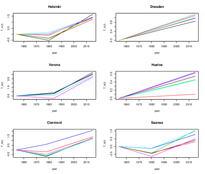
  Figure 11: Estimated trends (one color per state)

  

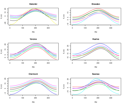
  Figure 12: Estimated seasonalities of temperature (one color per state)

  

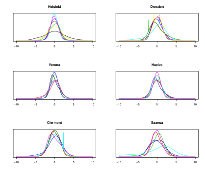
  Figure 13: Probability density functions of the random noises of the temperature (one color per state)

• Precipitation parameters (see Equation (5)):

  • the estimated seasonal components $1+\hat{\sigma}_{k}(t)$: the larger they are, the heavier the precipitations, if any. They are depicted in Figure 14. One can see that for all the considered sites, some of the states clearly exhibit a seasonal behaviour regarding the intensity of precipitations, in accordance with the right panel of Figure 7.

  • the weights of the Dirac masses, i.e. $\left(\hat{p}_{k0}\right)_{1\leq k\leq K}=\left(\sum_{m=1}^{M_{1}}\hat{p}_{km}\right)_{1\leq k\leq K}$: how dry or wet are the states. This can be compared to the left panel of Figure 7. For example, for the station of Verona,

    $$\left(\hat{p}_{k0}\right)_{1\leq k\leq K}=(0.88,0.68,0.93,0.95,0.09,0.09),$$

    so that the states $1$, $3$ and $4$ are mostly dry, whereas the states $5$ and $6$ are rainy.

  • the estimated parameters of the exponential distributions involved in each state, i.e.

    $$\left(\hat{\lambda}_{km}\right)_{\begin{subarray}{c}1\leq k\leq K\\ M_{1}+1\leq m\leq M\end{subarray}}.$$

    They represent the baseline intensity of rainfall (independently from the seasonal variations).

  

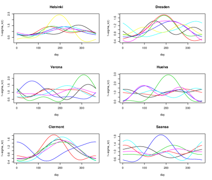
  Figure 14: Seasonalities in the precipitation intensity (one color per state)

Until now, we have not tested the model using simulations, but the estimated parameters are consistent with what we would expect from precipitations and temperatures. The validation of the model through simulations is the purpose of the next paragraph.

3.4.2 Validation of the model

Simulation

At this stage, for each site, we have ran the EM algorithm using our precipitation and temperature data as inputs, and we have at our disposal a vector of estimated parameters $\hat{\theta}$. This vector of parameters can be used to produce synthetic time series of temperature and precipitations $\left(Y_{t}^{\mathrm{sim}}\right)_{1\leq t\leq n}=\left(Y_{t}^{(1),\mathrm{sim}},Y_{t}^{(2),\mathrm{sim}}\right)_{1\leq t\leq n}$, where $n$ is the length of our observed time series. The simulation procedure is the following.

1. Simulate a sequence of states $\left(X_{t}^{\mathrm{sim}}\right)_{1\leq t\leq n}$ using the estimated transition matrices $\left(\hat{Q}(t)\right)_{1\leq t\leq n}$. The initial state $X_{1}^{\mathrm{sim}}$ can be chosen arbitrarily or drawn according to the stationary distribution of $\hat{Q}(1)$.

2. Given $\left(X_{t}^{\mathrm{sim}}\right)_{1\leq t\leq n}$, simulate $\left(Y_{t}^{\mathrm{sim}}\right)_{1\leq t\leq n}$. At time $t$, if $X_{t}^{\mathrm{sim}}=k$,

   1. Choose a component $m\in\{1,\dots,M\}$ according to the probability vector $\left(\hat{p}_{km}\right)_{1\leq m\leq M}$.

   2. Take $Y_{t}^{(2),\mathrm{sim}}$ as a realization of a $\mathcal{N}\left(\hat{T}_{k}(t)+\hat{S}_{k}(t)+\hat{\mu}_{km},\hat{\sigma}_{km}^{2}\right)$ distribution. This is our simulated temperature at time $t$.

   3. If $1\leq m\leq M_{1}$, then $Y_{t}^{(1),\mathrm{sim}}=0$, else take $Y_{t}^{(1),\mathrm{sim}}$ as a realization of a $\mathcal{E}\left(\frac{\hat{\lambda}_{km}}{1+\hat{\sigma}_{k}(t)}\right)$. This is our simulated precipitation at time $t$.

Note that the simulation algorithm gives insight into the reason why precipitation and temperature are dependent in our model: they always share the same state $k$, and the same mixture component $m$. This is crucial because we obviously do not want precipiation and temperature to be simulated independently.

Thus, using the above algorithm, we are able to simulate very easily and quickly a large number of synthetic time series of the same length as the observed ones. Using a standard laptop, we simulated $N_{\mathrm{sim}}=1000$ independent trajectories of length $n=22265$ in a few minutes, for each site. Now our goal is to compare these simulations to the observed times series, in order to check if our simulations are realistic, with regard to several criteria. Our validation procedure is divided into three parts, aiming to answer the three following questions:

• is the distribution of the precipitation process $(Y_{t}^{(1)})_{1\leq t\leq n}$ well reproduced?

• is the distribution of the temperature process $(Y_{t}^{(2)})_{1\leq t\leq n}$ well reproduced?

• is the dependence structure between precipitation and temperature well reproduced?

To this aim, we shall consider several statistics, or criteria of validation. These statistics will be computed from the data and from each of the $N_{\mathrm{sim}}$ simulated trajectory, thus providing a Monte-Carlo estimate of the distribution of each statistic under the model.

Temperature

Forgetting about the temporal aspect of the temperature time series, we can start by looking at the overall distribution of the temperatures. Figure 15 shows the quantile-quantile plot (QQ-plot) of observed versus simulated temperatures, for each site. Here we mix all the simulated values from the $1000$ trajectories of length $n=61\times 365=22265$. We see that the model can generate values that are more extreme than those observed in the data, both in the left and the right tail of the distribution. In the station of Huelva, the model has generated unrealistically cold values: $61$ values are below $-5$ whereas the minimum observed value is $0.4$. However, these are rare, considering the large number $N_{\mathrm{sim}}\times n$ of simulated values. Apart from that, the overall distribution is well reproduced.

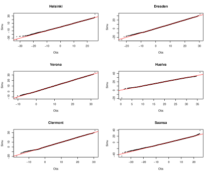
Figure 15: Quantile-quantile plots of observed vs simulated temperatures

Another way to look at the overall distribution of temperatures is to compute its observed quantiles and to compare them with the distributions of the quantiles generated by the model. For $\alpha\in(0,1)$, we can compute the observed empirical $\alpha$-th quantile, denoted by $q_{\alpha}^{\mathrm{obs}}$. Then we perform the same calculation for each simulation $s\in\{1,\dots,N_{\mathrm{sim}}\}$ and we obtain the quantiles $q_{\alpha}^{s}$. Finally, $q_{\alpha}^{\mathrm{obs}}$ is compared to the distribution of $(q_{\alpha}^{s})_{1\leq s\leq N_{\mathrm{sim}}}$ (estimated using a kernel density estimator). Figure 16 shows the example of the station of Clermont.

Figure 16: Observed (vertical lines) superimposed to the distribution of simulated (curve) quantiles of temperature for the station of Clermont. The dashed vertical lines are the bounds of a $95\%$ confidence interval.

Now let us have a look at some daily statistics, beginning with daily moments of the temperature distribution. For a day of year $t\in\{1,\dots,365\}$ (e.g. January 1st), we compute the empirical mean temperature at day $t$ by averaging over the years the temperatures observed this day:

$$\bar{Y}_{t}^{(2)}:=\frac{1}{N_{\mathrm{year}}}\sum_{i=1}^{N_{\mathrm{year}}}Y_{t+365(i-1)}^{(2)},$$

where $N_{\mathrm{year}}$ is the number of observed years (here $N_{\mathrm{year}}=61$). We perform the same calculation for each simulated scenario $s\in\{1,\dots,N_{\mathrm{sim}}\}$, that is

$$\bar{Y}_{t,s}^{(2)}:=\frac{1}{N_{\mathrm{year}}}\sum_{i=1}^{N_{\mathrm{year}}}Y_{t+365(i-1),s}^{(2)},$$

where $Y_{t,s}^{(2)}$ is the simulated temperature at time $t$ in the $s$-th simulation. Then, using $\left(\bar{Y}_{t,s}^{(2)}\right)_{1\leq s\leq N_{\mathrm{sim}}}$, we can estimate the distribution of the mean temperature at day $t$ under the model. To be specific, we compute the mean and a $95\%$ confidence interval based on quantiles from the values $\left(\bar{Y}_{t,s}^{(2)}\right)_{1\leq s\leq N_{\mathrm{sim}}}$. Finally, the same computations are performed for all $t\in\{1,\dots,365\}$, and for the next $3$ moments: standard deviation, skewness (asymmetry coefficient) and kurtosis, as shown in Figure 17 for the station of Dresden and Figure 18 for the station of Huelva. The first daily moments are well reproduced by the model. Figure 17 highlights the seasonality in the variability of temperature, as the standard deviation is maximal in winter, then decreases until it reaches its minimum at the end of summer, before increasing again. The shape of this seasonality is common to all the stations we studied, except Huelva (see Figure 18). This is consistent with what was observed in Figure 4. Another interesting observation is the asymmetry of the distribution of temperatures, measured by the third moment (skewness). Recall that a negative (resp. positive) skewness means that the distribution is skewed to the left (resp. right) whereas a skewness of $0$ means that the distribution is symmetric. The temperatures in Dresden clearly exhibit a seasonal behaviour in the asymmetry: the skewness is negative in winter and positive in summer. This reflects the presence of cold extremes in winter and hot extremes in summer. Using gaussian mixtures as emission distributions instead of simple gaussian distributions allows the model to reproduce this asymmetry. As Figure 18 shows, the station of Huelva, whose climate strongly differs from the climate of Dresden, does not exhibit the same seasonal behaviour, as the skewness curve is rather flat.

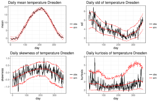
Figure 17: Daily moments of temperature for Dresden: observations (black line), mean of simulations (red solid line), $2.5\%$ and $97.5\%$ quantiles of simulations (red dashed lines)

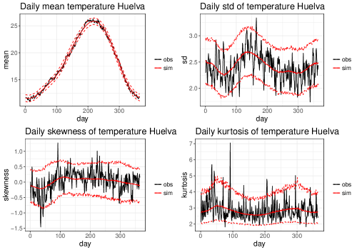
Figure 18: Daily moments of temperature for Huelva

Besides the moments, it is interesting to pay attention to the interannual minimum and maximum of daily mean temperature for each day. Precisely, for a day of year $t\in\{1,\dots,365\}$, the observed maximum is $\max_{1\leq i\leq N_{\mathrm{year}}}Y_{t+365(i-1)}^{(2)}$ and we estimate the distribution of this quantity under the model using the simulations, in the same way as we did for the moments. A similar computation is performed for the daily minima. This statistic is well reproduced by the model. As an example, Figure 19 shows the results for Clermont, Helsinki and Huelva.

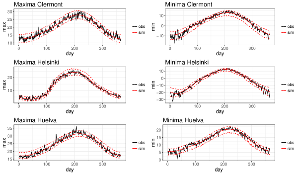
Figure 19: Interannual minimum and maximum of daily mean temperature for Clermont, Helsinki and Huelva

The temperatures do not form an independent process, as it is strongly autocorrelated. In our model, autocorrelation is introduced through the hidden Markov chain: even though the observations are generated independently conditionally to the states, they are not independent because the state process is autocorrelated. Hence the next criterion to be considered is the empirical auto-correlation of temperature with lags $1$, $2$ and $3$ days. Figure 20 shows that the model slightly underestimates the autocorrelations.

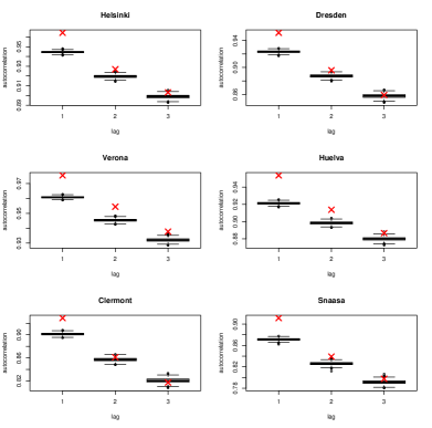
Figure 20: Autocorrelation of temperatures: the red crosses are the observed values and the boxplots are related to the different simulations

The last criterion that we are interested in regarding temperature is its persistence in extreme values. We fix some threshold $u$ (e.g. the $\alpha$-th quantile of temperature, with $\alpha$ close to $1$) and we consider the durations of the episodes exceeding $u$. Let us give an example. Assume that, for some $t\geq 2$, $Y_{t-1}^{(2)}\leq u$, $Y_{t}^{(2)}>u$, $Y_{t+1}^{(2)}>u$, $Y_{t+2}^{(2)}>u$ and $Y_{t+3}^{(2)}\leq u$. In such a case, we say that $\left(Y_{t}^{(2)},Y_{t+1}^{(2)},Y_{t+2}^{(2)}\right)$ is a hot cluster of length $3$ because the temperature remains for $3$ days above the threshold $u$. Thus the length of a cluster is a positive integer, possibly $1$. Similarly, we can define cold clusters by considering the times when the temperature drops below some low threshold. The results for hot clusters are shown by Figure 21. Here the threshold $u$ is the $95$-th percentile (hence it varies according to the site). Clearly, for all sites, the model produces too many clusters of length $1$, therefore not enough longer clusters. We tried various thresholds between the $90$-th and the $99$-th quantiles and the same conclusion can be drawn. Thus the persistence in extreme values is underestimated by the model. This is not surprising, considering that the autocorrelations of temperature are slightly underestimated too (see Figure 20). The same issue appears when we consider cold clusters, as we can see in Figure 22.

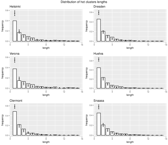
Figure 21: Distribution of the lengths of the hot clusters. The threshold is the $95$-th percentile. White bars: observed values. Errorbars: $95\%$ confidence interval based on the simulations.

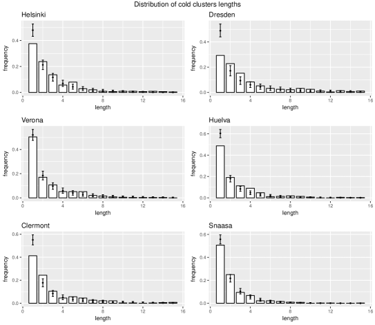
Figure 22: Distribution of the lengths of the cold clusters. The threshold is the $5$-th percentile. White bars: observed values. Errorbars: $95\%$ confidence interval based on the simulations.

Precipitation

Figure 23 shows the quantile-quantile plots of precipitation, for each of the six sites. To be specific, we plotted the $\alpha$-quantiles of observed precipitations versus the corresponding simulated $\alpha$-quantiles, for $\alpha\in\leavevmode\nobreak\ \{\frac{i}{1000},\,1\leq\leavevmode\nobreak\ i\leq\leavevmode\nobreak\ 999\}$. As the distribution of precipitations is very asymmetric, we zoom-in to the $\alpha$ greater than $0.9$ (see Figure 24). As we can see, the overall distribution of precipitations, including its tail, is well reproduced. It is also interesting to note that our model is able to simulate precipitation values that are larger than all the observed values. As an example, the maximum observd value of daily precipitation in Helsinki is $79.3$ mm, but $14$ of the $1000$ simulated trajectories include a larger value, the maximum being $110.7$ mm. This is one of the assets of model compared to models based on resampling. However, the exponential distribution being unbounded, performing a large number of simulations sometimes leads to unrealistic precipitations values.

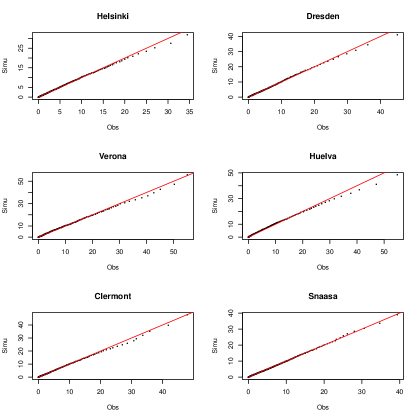
Figure 23: Precipitation quantile-quantile plots.

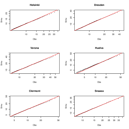
Figure 24: Precipitation quantile-quantile plots, tail of distribution (logarithmic scale)

We can also check the distributions of the simulated quantiles. As an example, Figure 25 shows the distributions of some upper quantiles for the station of Snåsa, and their observed counterparts.

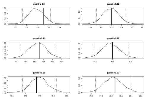
Figure 25: Observed (vertical lines) superimposed to the distribution of simulated (curve) quantiles of precipitation for the station of Snåsa. The dashed vertical lines are the bounds of a $95\%$ confidence interval.

As we did for temperature, we estimate the daily moments of precipitations. We also estimate the daily frequencies of precipitations by computing, for $t\in\{1,\dots,T\}$, an estimate of $\mathbb{P}(Y_{t}^{(1)}>0)$ as

$$\frac{1}{N_{\mathrm{year}}}\sum_{i=1}^{N_{\mathrm{year}}}\mathbf{1}_{Y_{t+365(i-1)}^{(1)}>0},$$

and the maxima of daily precipitations totals:

$$\max_{1\leq i\leq N_{\mathrm{year}}}Y_{t+365(i-1)}^{(1)},\quad 1\leq t\leq 365$$

Using the simulations, we estimate the distribution of these statistics under the model. The results are presented in Figure 26 for the station of Helsinki, together with the first four daily moments. The seasonalities in the intensity and in the frequency of precipitations are well reproduced by the model.

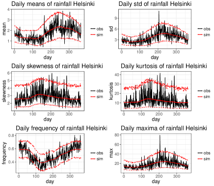
Figure 26: Daily moments of precipitations

A dry spell is a period of time during which it does not rain. When there are $d$ consecutive days without rain and non-zero precipitations on the $(d+1)$-th day, this constitutes a dry spell of length $d$. Similarly, we define wet spells as consecutive days with non-zero precipitations. Figures 27 and 28 show the observed and simulated distributions of dry and wet spells. The lengths of dry spells are quite well reproduced by the model but for some stations (e.g. Clermont), the model clearly underestimates the number of wet spells longer than one day.

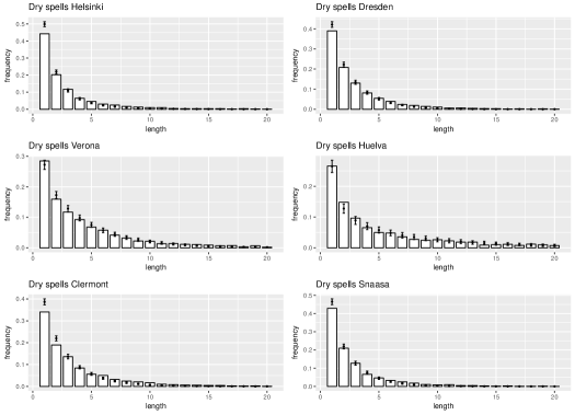
Figure 27: Distribution of the length of dry spells. White bars: observed values. Errorbars: $95\%$ confidence interval based on the simulations.

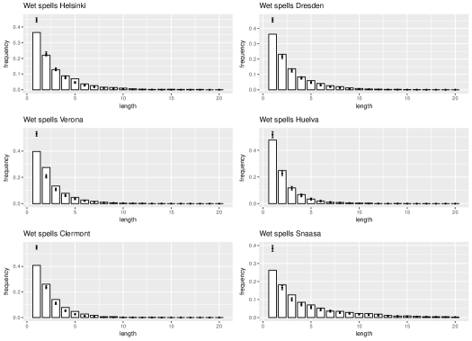
Figure 28: Distribution of the length of wet spells. White bars: observed values. Errorbars: $95\%$ confidence interval based on the simulations.

Stochastic precipitations generators often underestimate the interannual variability of precipitations (Katz and Parlange, 1998). Thus we focus on yearly rainfall and we look at its interannual variability. The histograms in Figure 29 are the observed distributions of yearly precipitations (thus each histogram has been computed with $61$ observations). The lines are the kernel density estimations of simulated yearly precipitations. We have performed the same computations with monthly precipitations (see Figure 30 for the station of Clermont). Our model does not underestimate interannual variability, as it is able to generate rainy as well as dry years or months.

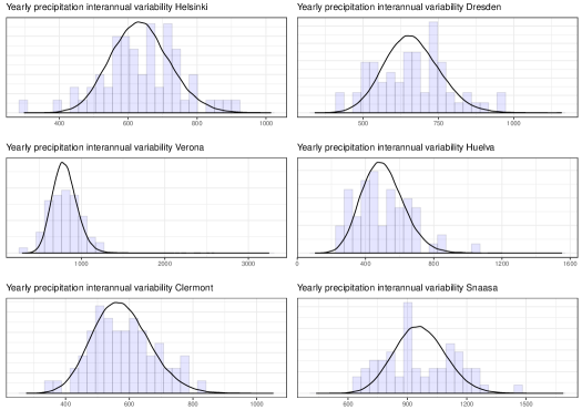
Figure 29: Interannual variability of yearly precipitations

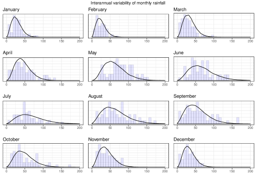
Figure 30: Interannual variability of monthly precipitations

Temperature and precipitation coupling

At this stage, we have assessed the performance of our model for temperature and precipitations separately. We shall now concentrate on the relationship between these two variables, as they are not independent. Figure 31 shows that the model provides realistic monthly correlations between temperature and precipitations.

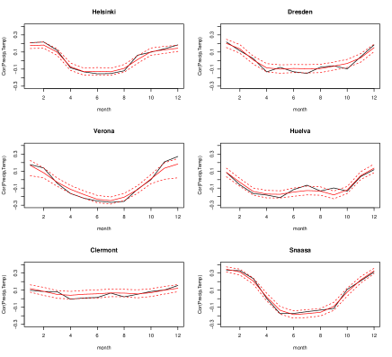
Figure 31: Monthly correlations between temperature and precipitations. Black solid line: observed. Red solid line: mean of simulations. Red dashed lines: $95\%$ confidence interval from simulations.

However, a better representation of the relationship between temperature and precipitations can be obtained. For example, the probability of observing precipitations varies with temperature: for $u,v\in\mathbb{R}$, in general,

$$\mathbb{P}\left(Y_{t}^{(1)}>0\mid Y_{t}^{(2)}=u\right)\neq\mathbb{P}\left(Y_{t}^{(1)}>0\mid Y_{t}^{(2)}=v\right).$$

Similarly, the expected value of non-zero precipitation depends on temperature: for $u,v\in\mathbb{R}$, in general,

$$\mathbb{E}\left[Y_{t}^{(1)}\mid Y_{t}^{(1)}>0,Y_{t}^{(2)}=u\right]\neq\mathbb{E}\left[Y_{t}^{(1)}\mid Y_{t}^{(1)}>0,Y_{t}^{(2)}=v\right].$$

Note that the quantities $\mathbb{P}\left(Y_{t}^{(1)}>0\mid Y_{t}^{(2)}=u\right)$ and $\mathbb{E}\left[Y_{t}^{(1)}\mid Y_{t}^{(1)}>0,Y_{t}^{(2)}=u\right]$ depend not only on $u$ but also on $t$ as the process $\left(Y_{t}^{(1)},Y_{t}^{(2)}\right)_{t\geq 1}$ is not stationary.

Let $\mathcal{K}$ be the gaussian kernel defined by $\mathcal{K}(x)=\exp\left(-\frac{x^{2}}{2}\right)$. For $y\in\mathbb{R}$ and a bandwidth $h>0$, we consider the following statistics.

$$r(y):=\frac{\sum_{t=1}^{n}\mathcal{K}\left(\frac{Y_{t}^{(2)}-y}{h}\right)\mathbf{1}_{Y_{t}^{(1)}>0}}{\sum_{t=1}^{n}\mathcal{K}\left(\frac{Y_{t}^{(2)}-y}{h}\right)}$$

$$R(y):=\frac{\sum_{t=1}^{n}\mathcal{K}\left(\frac{Y_{t}^{(2)}-y}{h}\right)Y_{t}^{(1)}}{\sum_{t=1}^{n}\mathcal{K}\left(\frac{Y_{t}^{(2)}-y}{h}\right)\mathbf{1}_{Y_{t}^{(1)}>0}}$$

If we had a sample $\left(Y_{t}^{(1)},Y_{t}^{(2)}\right)_{1\leq t\leq n}$ of i.i.d. copies of $\left(Y^{(1)},Y^{(2)}\right)$, then $r(y)$ would be an estimator of $\mathbb{P}\left(Y^{(1)}>0\mid Y^{(2)}=y\right)$ and $R(y)$ would be an estimator of $\mathbb{E}\left[Y^{(1)}\mid Y^{(1)}>0,Y^{(2)}=y\right]$. Although this is not the case, these statistics still provide some information on the dependence between precipitation occurrence and temperature and it is interesting to see how the model behaves with respect to $r(y)$ and $R(y)$. Therefore, the functions $y\mapsto r(y)$ and $y\mapsto R(y)$ are computed from the observations and from each of the $1000$ bivariate simulations. Figures 32 and 33 show the results for the six stations (with $h=2$). Here again, the model is performing well with regard to these statistics.

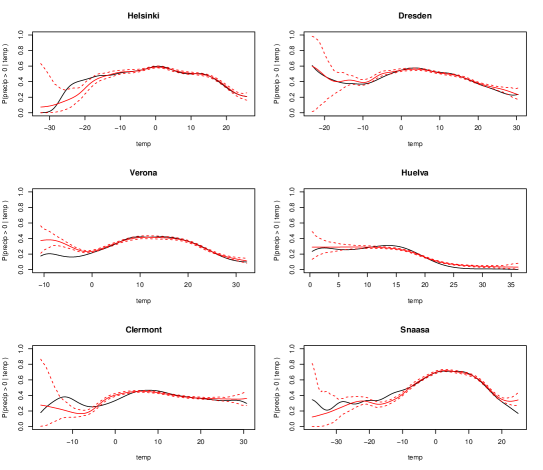
Figure 32: Graph of the function $y\mapsto r(y)$. Solid black curve: computation on the observations. Solid red curve: mean of the simulated values. Dashed red curves: $95\%$ confidence interval based on simulations.

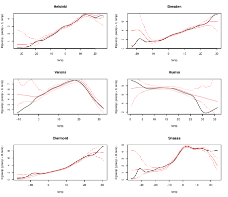
Figure 33: Graph of the function $y\mapsto R(y)$. Solid black curve: computation on the observations. Solid red curve: mean of the simulated values. Dashed red curves: $95\%$ confidence interval based on simulations.

For $t\in\{1,\dots n\}$, we denote by $\bar{t}\in\{1,\dots,365\}$ its representative modulo $365$, that is the day of year. For $t,s\in\{1,\dots,n\}$, let

$$\|t-s\|:=\min(|\bar{t}-\bar{s}|,365-|\bar{t}-\bar{s}|)$$

be the cyclic distance between days $t$ and $s$, that is the number of days between the corresponding days of year. For $h_{1},h_{2}>0$, $y\in\mathbb{R}$ and $t\in\{1,\dots,365\}$, let us define

$$r(t,y):=\frac{\sum_{s=1}^{n}\mathcal{K}\left(\frac{\|t-s\|}{h_{1}}\right)\mathcal{K}\left(\frac{y-Y^{(2)}_{s}}{h_{2}}\right)\mathbf{1}_{Y_{s}^{(1)}>0}}{\sum_{s=1}^{n}\mathcal{K}\left(\frac{\|t-s\|}{h_{1}}\right)\mathcal{K}\left(\frac{y-Y^{(2)}_{s}}{h_{2}}\right)},$$

and

$$R(t,y):=\frac{\sum_{s=1}^{n}\mathcal{K}\left(\frac{\|t-s\|}{h_{1}}\right)\mathcal{K}\left(\frac{y-Y^{(2)}_{s}}{h_{2}}\right)Y_{s}^{(1)}}{\sum_{s=1}^{n}\mathcal{K}\left(\frac{\|t-s\|}{h_{1}}\right)\mathcal{K}\left(\frac{y-Y^{(2)}_{s}}{h_{2}}\right)\mathbf{1}_{Y_{s}^{(1)}>0}}.$$

Then $r(t,y)$ is a proxy for $\mathbb{P}\left(Y_{t}^{(1)}>0\mid Y_{t}^{(2)}=y\right)$ and $R(t,y)$ is a proxy for $\mathbb{E}\left[Y_{t}^{(1)}\mid Y_{t}^{(1)}>0,Y_{t}^{(2)}=u\right]$. Hence we use these statistics as validation criteria. Figures 34 and 35 show the results for the station of Verona for four different days of year. Results are in general satisfying and demonstrate a realistic coupling between the two variables.

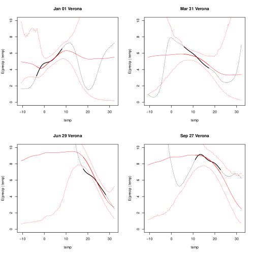
Figure 34: Graphs of the function $y\mapsto r(t,y)$ for different values of $t$ (day of year) in Verona. Solid black curve: computation on the observations. Solid red curve: mean of the simulated values. Dashed red curves: $95\%$ confidence interval based on simulations. The dashed black curve is an extrapolation of $y\mapsto r(t,y)$ outside the observed range of temperature at day of year $t$: although the computation is feasible, it is not relevant.

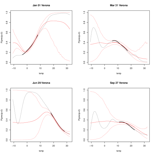
Figure 35: Graphs of the function $y\mapsto R(t,y)$ for different values of $t$ (day of year) in Verona. Solid black curve: computation on the observations. Solid red curve: mean of the simulated values. Dashed red curves: $95\%$ confidence interval based on simulations. The dashed black curve is an extrapolation of $y\mapsto r(t,y)$ outside the observed range of temperature at day of year $t$: although the computation is feasible, it is not relevant.

4 Conclusion

We introduced a seasonal hidden Markov model for the joint modeling of daily temperature and precipitations. The non-homogeneity of the underlying Markov chain allows the model to account for the complex seasonal features of these weather variables, as well as climate change, in a unified framework, without resorting to pre-processing the data or fitting multiple models. Our model can be used as a stochastic weather generator, as it can quickly generate realistic synthetic time series of temperature and precipitations, at a given site. Considering many criteria of interest, we showed that these simulations closely reproduce the behaviour of the data, be it the marginal distributions of the two variables or their dependence relationships. Furthermore, we showed that investigating the estimated parameters of the model leads to giving a posteriori a physical intepretation to the hidden states, thus avoiding the pitfall of a black box model. We also proved the robustness of our model by testing it on different sites with various climates.

Several extensions of our model can be considered and be the subject of future works. First, we noted that in many cases, it fails to reproduce correctly the extreme heat or cold episodes, and the dry and rainy spells. This flaw can be caused by a lack of autocorrelation and could be adressed by adding autoregression in the process. Using our notations, the distribution of $Y_{t}$ could depend on $t$, $Y_{t-1}$ and $X_{t}$ instead of just being a function of $t$ and $X_{t}$. Then, extreme values of temperature and precipitations can be investigated more closely. We did not focus on this particular point but some applications need a fine modeling of extremes. To this aim, it may be necessary to choose other emission distributions, even though we showed that the upper quantiles of temperature and precipitations were well reproduced. In order to apply the model to sites where there is a sensible trend in the distibution of precipitations, it would have to be modified. Finally, the structure of our model can easily be extended to more variables (e.g. wind speed), the main difficulty being the choice of the emission distributions.

References

- Ailliot and Monbet (2012) Pierre Ailliot and Valérie Monbet. Markov-switching autoregressive models for wind time series. Environmental Modelling & Software, 30:92–101, 2012.
- Ailliot and Pene (2015) Pierre Ailliot and Françoise Pene. Consistency of the maximum likelihood estimate for non-homogeneous markov–switching models. ESAIM: Probability and Statistics, 19:268–292, 2015.
- Ailliot et al. (2015) Pierre Ailliot, Denis Allard, Valérie Monbet, and Philippe Naveau. Stochastic weather generators: an overview of weather type models. Journal de la Société Française de Statistique, 156(1):101–113, 2015.
- Alexandrovich et al. (2016) Grigory Alexandrovich, Hajo Holzmann, and Anna Leister. Nonparametric identification and maximum likelihood estimation for hidden markov models. Biometrika, 103(2):423–434, 2016.
- Allman et al. (2009) Elizabeth S Allman, Catherine Matias, and John A Rhodes. Identifiability of parameters in latent structure models with many observed variables. The Annals of Statistics, pages 3099–3132, 2009.
- Baum and Petrie (1966) Leonard E Baum and Ted Petrie. Statistical inference for probabilistic functions of finite state markov chains. The annals of mathematical statistics, 37(6):1554–1563, 1966.
- Bellone et al. (2000) Enrica Bellone, James P Hughes, and Peter Guttorp. A hidden Markov model for downscaling synoptic atmospheric patterns to precipitation amounts. Climate research, 15(1):1–12, 2000.
- Benth and Šaltytė Benth (2011) Fred Espen Benth and Jūratė Šaltytė Benth. Weather derivatives and stochastic modelling of temperature. International Journal of Stochastic Analysis, 2011, 2011.
- Biernacki et al. (2000) Christophe Biernacki, Gilles Celeux, and Gérard Govaert. Assessing a mixture model for clustering with the integrated completed likelihood. IEEE transactions on pattern analysis and machine intelligence, 22(7):719–725, 2000.
- Biernacki et al. (2003) Christophe Biernacki, Gilles Celeux, and Gérard Govaert. Choosing starting values for the em algorithm for getting the highest likelihood in multivariate gaussian mixture models. Computational Statistics & Data Analysis, 41(3):561–575, 2003.
- Campbell and Diebold (2005) Sean D Campbell and Francis X Diebold. Weather forecasting for weather derivatives. Journal of the American Statistical Association, 100(469):6–16, 2005.
- Dempster et al. (1977) Arthur P Dempster, Nan M Laird, and Donald B Rubin. Maximum likelihood from incomplete data via the EM algorithm. Journal of the Royal Statistical Society. Series B (methodological), pages 1–38, 1977.
- Diehn et al. (2018) Manuel Diehn, Axel Munk, and Daniel Rudolf. Maximum likelihood estimation in hidden markov models with inhomogeneous noise. arXiv preprint arXiv:1804.04034, 2018.
- Douc et al. (2011) Randal Douc, Eric Moulines, Jimmy Olsson, Ramon Van Handel, et al. Consistency of the maximum likelihood estimator for general hidden markov models. the Annals of Statistics, 39(1):474–513, 2011.
- Flecher et al. (2010) C Flecher, P Naveau, D Allard, and N Brisson. A stochastic daily weather generator for skewed data. Water Resources Research, 46(7), 2010.
- Gassiat et al. (2016) Elisabeth Gassiat, Alice Cleynen, and Stéphane Robin. Finite state space non parametric hidden markov models are in general identifiable. Statistics and Computing, 26(1–2):61–71, 2016.
- Hughes and Guttorp (1994) James P Hughes and Peter Guttorp. A class of stochastic models for relating synoptic atmospheric patterns to regional hydrologic phenomena. Water resources research, 30(5):1535–1546, 1994.
- Hughes et al. (1999) James P Hughes, Peter Guttorp, and Stephen P Charles. A non-homogeneous hidden Markov model for precipitation occurrence. Journal of the Royal Statistical Society: Series C (Applied Statistics), 48(1):15–30, 1999.
- Katz and Parlange (1998) Richard W Katz and Marc B Parlange. Overdispersion phenomenon in stochastic modeling of precipitation. Journal of Climate, 11(4):591–601, 1998.
- Kirshner (2005) Sergey Kirshner. Modeling of multivariate time series using hidden Markov models. PhD thesis, University of California, Irvine, 2005.
- Lehéricy (to appear) Luc Lehéricy. Consistent order estimation for nonparametric hidden Markov models. Bernoulli, to appear.
- Lennartsson et al. (2008) Jan Lennartsson, Anastassia Baxevani, and Deliang Chen. Modelling precipitation in sweden using multiple step Markov chains and a composite model. Journal of hydrology, 363(1):42–59, 2008.
- Leroux (1992) Brian G Leroux. Maximum-likelihood estimation for hidden markov models. Stochastic processes and their applications, 40(1):127–143, 1992.
- Mraoua (2007) Mohammed Mraoua. Temperature stochastic modeling and weather derivatives pricing: empirical study with moroccan data. Afrika Statistika, 2(1), 2007.
- Peleg et al. (2017) Nadav Peleg, Simone Fatichi, Athanasios Paschalis, Peter Molnar, and Paolo Burlando. An advanced stochastic weather generator for simulating 2-d high-resolution climate variables. Journal of Advances in Modeling Earth Systems, 2017.
- Pohle et al. (2017) Jennifer Pohle, Roland Langrock, Floris van Beest, and Niels Martin Schmidt. Selecting the number of states in hidden Markov models-pitfalls, practical challenges and pragmatic solutions. arXiv preprint arXiv:1701.08673, 2017.
- Pouzo et al. (2016) Demian Pouzo, Zacharias Psaradakis, and Martin Sola. Maximum likelihood estimation in possibly misspecified dynamic models with time inhomogeneous markov regimes. 2016.
- Richardson (1981) Clarence W Richardson. Stochastic simulation of daily precipitation, temperature, and solar radiation. Water resources research, 17(1):182–190, 1981.
- Schwarz et al. (1978) Gideon Schwarz et al. Estimating the dimension of a model. The annals of statistics, 6(2):461–464, 1978.
- Touron (2018) Augustin Touron. Consistency of the maximum likelihood estimator in seasonal hidden markov models. arXiv preprint arXiv:1802.08161, 2018.
- Vrac et al. (2007) Mathieu Vrac, Michael Stein, and Katharine Hayhoe. Statistical downscaling of precipitation through nonhomogeneous stochastic weather typing. Climate Research, 34(3):169–184, 2007.
- Wilks and Wilby (1999) Daniel S Wilks and Robert L Wilby. The weather generation game: a review of stochastic weather models. Progress in physical geography, 23(3):329–357, 1999.
- Zucchini and Guttorp (1991) Walter Zucchini and Peter Guttorp. A hidden Markov model for space-time precipitation. Water Resources Research, 27(8):1917–1923, 1991.