Proton–philic spin–dependent inelastic Dark Matter (pSIDM) as a viable explanation of DAMA/LIBRA–phase2

Abstract

We show that the Weakly Interacting Massive Particle scenario of proton-philic spin-dependent inelastic Dark Matter (pSIDM) can still provide a viable explanation of the observed DAMA modulation amplitude in compliance with the constraints from other experiments after the release of the DAMA/LIBRA–phase2 data and including the recent bound from COSINE–100, that uses the same $NaI$ target of DAMA. The pSIDM scenario provided a viable explanation of DAMA/LIBRA–phase1 both for a Maxwellian WIMP velocity distribution and in a halo–independent approach. At variance with DAMA/LIBRA–phase1, for which the modulation amplitudes showed an isolated maximum at low energy, the DAMA/LIBRA–phase2 spectrum is compatible to a monotonically decreasing one. Moreover, due to its lower threshold, it is sensitive to WIMP–iodine interactions at low WIMP masses. Due to the combination of these two effects pSIDM can now explain the yearly modulation observed by DAMA/LIBRA only when the WIMP velocity distribution departs from a standard Maxwellian. In this case the WIMP mass $m_{\chi}$ and mass splitting $\delta$ fall in the approximate ranges 7 GeV $\mathrel{\mathop{\kern 0.0pt\hbox to0.0pt{\raise 0.86108pt\hbox{$<$}\hss}}\lower 3.87495pt\hbox{\kern-1.90002pt$\sim$}}m_{\chi}\mathrel{\mathop{\kern 0.0pt\hbox to0.0pt{\raise 0.86108pt\hbox{$<$}\hss}}\lower 3.87495pt\hbox{\kern-1.90002pt$\sim$}}$ 17 GeV and 18 keV$\mathrel{\mathop{\kern 0.0pt\hbox to0.0pt{\raise 0.86108pt\hbox{$<$}\hss}}\lower 3.87495pt\hbox{\kern-1.90002pt$\sim$}}\delta\mathrel{\mathop{\kern 0.0pt\hbox to0.0pt{\raise 0.86108pt\hbox{$<$}\hss}}\lower 3.87495pt\hbox{\kern-1.90002pt$\sim$}}$29 keV. The recent COSINE–100 bound is naturally evaded in the pSDIM scenario due to its large expected modulation fractions.

I Introduction

About one quarter of the total mass density of the Universe Ade et al. (2014) and more than 90% of the halo of our Galaxy are believed to be constituted by Dark Matter (DM) and Weakly Interacting Massive Particles (WIMPs) are one of the most popular candidates to compose it. The scattering rate of DM WIMPs in a terrestrial detector is expected to present a modulation with a period of one year due to the Earth revolution around the Sun Drukier et al. (1986).

The DAMA collaboration Bernabei et al. (2008, 2010, 2013) has been measuring for more than 15 years a yearly modulation effect in their sodium iodide target. Such effect has a statistical significance of more than $9\sigma$ and is consistent with what is expected from DM WIMPs. However, in the most popular WIMP scenarios the DAMA modulation appears incompatible with the results from many other DM experiments that have failed to observe any signal so far.

This has lead to extend the class of WIMP models. In particular, one of the few phenomenological scenarios that have been shown to explain the DAMA effect in agreement with the constraints from other experiments is proton–philic spin–dependent inelastic Dark Matter (pSIDM) Scopel and Yoon (2016); Scopel and Yu (2017) for WIMP masses 10 ${\rm GeV}\mathrel{\mathop{\kern 0.0pt\hbox to0.0pt{\raise 0.86108pt\hbox{$<$}\hss}}\lower 3.87495pt\hbox{\kern-1.90002pt$\sim$}}m_{\chi}\mathrel{\mathop{\kern 0.0pt\hbox to0.0pt{\raise 0.86108pt\hbox{$<$}\hss}}\lower 3.87495pt\hbox{\kern-1.90002pt$\sim$}}$ 30 ${\rm GeV}$ and a mass splitting 10 keV $\mathrel{\mathop{\kern 0.0pt\hbox to0.0pt{\raise 0.86108pt\hbox{$<$}\hss}}\lower 3.87495pt\hbox{\kern-1.90002pt$\sim$}}\delta\mathrel{\mathop{\kern 0.0pt\hbox to0.0pt{\raise 0.86108pt\hbox{$<$}\hss}}\lower 3.87495pt\hbox{\kern-1.90002pt$\sim$}}$ 30 keV.

Recently the DAMA collaboration has released first result from the upgraded DAMA/LIBRA-phase2 experiment Bernabei et al. (2018). Compared to the previous data the two most important improvements are that now the exposure has almost doubled and that the energy threshold has been lowered from 2 keV electron–equivalent (keVee) to 1 keVee. Moreover, an important difference with the result of DAMA/LIBRA–phase1 is that the new DAMA/LIBRA–phase2 spectrum of modulation amplitudes no longer shows a maximum, but is rather monotonically decreasing with energy. Moreover, several direct WIMP searches have improved their bounds, including the COSINE–100 collaboration Adhikari et al. (2018a) that has recently published an exclusion plot about a factor of two below the DAMA region using 106 kg of $NaI$, the same target of DAMA, assuming an elastic, spin–independent isoscalar WIMP nucleus interaction and a WIMP Maxwellian velocity distribution. In light of these differences in the present paper we wish to update the assessment of pSIDM with the new DAMA/LIBRA–phase2 data, both in a scenario where the WIMP speed distribution $f(v)$ is given by a standard Maxwellian and using a halo–independent approach where $f(v)$ is not fixed.

In the present paper we will show that pSIDM can still provide a viable explanation of the modulation effect after DAMA/LIBRA-phase2. In particular, while the pSIDM scenario was able to explain DAMA/LIBRA–phase1 both for a Maxwellian $f(v)$ and in a halo–independent approach Scopel and Yoon (2016); Scopel and Yu (2017) in the present paper we will show that for a Maxwellian WIMP velocity distribution it provides a poor fit to the new DAMA data and for a range of the pSIDM parameters in tension with the null results of other DM searches. On the other hand in a halo–independent approach the pSIDM scenario is still viable. Moreover, we will show that the recent COSINE–100 bound is naturally evaded in the pSDIM scenario due to its large expected modulation fractions.

The paper is organized as follows. In Section II we outline the main features of the pSIDM scenario; in Section  III.1 we analyze the DAMA data adopting a standard Maxwellian for the WIMP velocity distribution; in Section III.2 we analyze the DAMA data in a halo–independent approach. In appendixIV we provide some details on how the experimental constraints on pSIDM have been obtained.

II The pSIDM scenario

The most stringent bounds on an interpretation of the DAMA effect in terms of WIMP–nuclei scatterings are obtained by detectors using xenon (XENON1T Aprile et al. (2018), PANDAX–II Cui et al. (2017), LUX Akerib et al. (2016)) and germanium (CDMS Ahmed et al. (2011); Agnese et al. (2014a, b, 2015)) whose spin is mostly originated by an unpaired neutron while, on the other hand, both sodium and iodine in DAMA have an unpaired proton. This implies that if the WIMP particle interacts with ordinary matter predominantly via a spin–dependent coupling which is suppressed for neutrons it can explain the DAMA effect in compliance with xenon and germanium bounds Ullio et al. (2001); Del Nobile et al. (2015). Actually, present limits from xenon detectors require to tune the neutron/proton coupling ratio $c^{n}/c^{p}$ to a small but non–vanishing value Scopel and Yoon (2016). In the following we will adopt the xenon–phobic combination $c^{n}/c^{p}$=-0.028, that minimizes the xenon spin–dependent response using the nuclear structure functions in Anand et al. (2014) . This scenario is still constrained by droplet detectors and bubble chambers (COUPP Behnke et al. (2012), PICASSO Behnke et al. (2017), PICO-60 Amole et al. (2017))) which all use nuclear targets with an unpaired proton (${}^{19}F$ and/or ${}^{127}I$). As a consequence, this class of experiments rules out a DAMA explanation in terms of WIMPs with a spin–dependent coupling to protons Del Nobile et al. (2015); Amole et al. (2015); Scopel and Yoon (2016).

In Ref. Scopel and Yoon (2016) Inelastic Dark Matter Tucker-Smith and Weiner (2001) (IDM) was proposed to reconcile the above scenario to fluorine detectors. In IDM a DM particle $\chi_{1}$ of mass $m_{\chi_{1}}=m_{\chi}$ interacts with atomic nuclei exclusively by up–scattering to a second heavier state $\chi_{2}$ with mass $m_{\chi_{2}}=m_{\chi}+\delta$. A peculiar feature of IDM is that there is a minimal WIMP incoming speed in the lab frame matching the kinematic threshold for inelastic upscatters and given by:

$$v_{min}^{*}=\sqrt{\frac{2\delta}{\mu_{\chi N}}},$$ (1)

with $\mu_{\chi N}$ the WIMP–nucleus reduced mass. This quantity corresponds to the lower bound of the minimal velocity $v_{min}$ (also defined in the lab frame) required to deposit a given recoil energy $E_{R}$ in the detector:

$$v_{min}=\frac{1}{\sqrt{2m_{N}E_{R}}}\left|\frac{m_{N}E_{R}}{\mu_{\chi N}}+\delta\right|,$$ (2)

with $m_{N}$ the nuclear mass. In particular, indicating with $v_{min}^{*Na}$ and $v_{min}^{*F}$ the values of $v_{min}^{*}$ for sodium and fluorine, and with $v_{esc}$ the WIMP escape velocity, constraints from WIMP–fluorine scattering events in droplet detectors and bubble chambers can be evaded when the WIMP mass $m_{\chi}$ and the mass gap $\delta$ are chosen in such a way that the hierarchy:

$$v_{min}^{*Na}<v_{esc}^{lab}<v_{min}^{*F},$$ (3)

is achieved, since in such case WIMP scatterings off fluorine turn kinematically forbidden while those off sodium can still serve as an explanation to the DAMA effect. So the pSIDM mechanism rests on the trivial observation that the velocity $v_{min}^{*}$ for fluorine is larger than that for sodium.

III Analysis

The expected rate in a given visible energy bin $E_{1}^{\prime}\leq E^{\prime}\leq E_{2}^{\prime}$ of a direct detection experiment is given by:

$$R_{[E_{1}^{\prime},E_{2}^{\prime}]}(t) = MT_{exp}\int_{E_{1}^{\prime}}^{E_{2}^{\prime}}\frac{dR}{dE^{\prime}}(t)\,dE^{\prime}$$

$$\frac{dR}{dE^{\prime}}(t) = \sum_{T}\int_{0}^{\infty}\frac{dR_{\chi T}(t)}{dE_{ee}}{\cal G}_{T}(E^{\prime},E_{ee})\epsilon(E^{\prime})\,dE_{ee}$$

$$E_{ee} = q(E_{R})E_{R},$$ (4)

with $\epsilon(E^{\prime})\leq 1$ the experimental efficiency/acceptance. In the equations above $E_{R}$ is the recoil energy deposited in the scattering process (indicated in keVnr), while $E_{ee}$ (indicated in keVee) is the fraction of $E_{R}$ that goes into the experimentally detected process (ionization, scintillation, heat) and $q(E_{R})$ is the quenching factor, ${\cal G_{T}}(E^{\prime},E_{ee}=q(E_{R})E_{R})$ is the probability that the visible energy $E^{\prime}$ is detected when a WIMP has scattered off an isotope $T$ in the detector target with recoil energy $E_{R}$, $M$ is the fiducial mass of the detector and $T_{exp}$ the live–time exposure of the data taking.

In Eq.(4) the differential recoil rate $dR_{\chi T}(t)/dE_{R}$ is given by:

$$\frac{dR_{\chi T}}{dE_{R}}(t)=\sum_{T}N_{T}\frac{\rho_{\mbox{\tiny WIMP}}}{m_{\mbox{\tiny WIMP}}}\int_{v_{min}}d^{3}v_{T}f(\vec{v}_{T},t)v_{T}\frac{d\sigma_{T}}{dE_{R}},$$ (5)

where $\rho_{\mbox{\tiny WIMP}}$ is the local WIMP mass density in the neighborhood of the Sun (in the following we will assume the standard value $\rho_{\mbox{\tiny WIMP}}$=0.3 GeV/cm³), $f(\vec{v}_{T},t)$ is the WIMP velocity distribution (whose boost in the Earth rest frame induces a time–dependence), $N_{T}$ the number of the nuclear targets of species $T$ in the detector (the sum over $T$ applies in the case of more than one target), while:

$$\frac{d\sigma_{T}}{dE_{R}}=\frac{\sigma_{0}}{E_{R}^{max}}=\frac{2m_{T}}{4\pi v_{T}^{2}}\left[\frac{1}{2j_{\chi}+1}\frac{1}{2j_{T}+1}|\mathcal{M}_{T}|^{2}\right],$$ (6)

with $m_{T}$ the mass of the nuclear target, $j_{\chi}$=1/2 the spin of the WIMP, $E_{R}^{max}=2\mu_{\chi T}^{2}/m_{T}v_{T}^{2}$ and $\sigma_{0}$ the point–like WIMP–nucleon cross section. In the following, for the calculation of the squared amplitude $|\mathcal{M}_{T}|^{2}$ we will use the spin–dependent nuclear form factors from Anand et al. (2014) for all nuclei with the exception of caesium and tungsten, for which we follow the same procedure adopted in Appendix C of Kang et al. (2018b).

In particular, in each visible energy bin DAMA is sensitive to the yearly modulation amplitude $S_{m}$, defined as the cosine transform of $R_{[E_{1}^{\prime},E_{2}^{\prime}]}(t)$:

$$S_{m,[E_{1}^{\prime},E_{2}^{\prime}]}\equiv\frac{2}{T_{0}}\int_{0}^{T_{0}}\cos\left[\frac{2\pi}{T_{0}}(t-t_{0})\right]R_{[E_{1}^{\prime},E_{2}^{\prime}]}(t)dt,$$ (7)

with $T_{0}$=1 year and $t_{0}$=2^nd June, while other experiments put upper bounds on the time average $S_{0}$:

$$S_{0,[E_{1}^{\prime},E_{2}^{\prime}]}\equiv\frac{1}{T_{0}}\int_{0}^{T_{0}}R_{[E_{1}^{\prime},E_{2}^{\prime}]}(t)dt.$$ (8)

III.1 Maxwellian analysis

In this Section we assume that the WIMP velocity distribution in the Galactic rest frame is a standard isotropic Maxwellian at rest, truncated at the escape velocity $v_{\rm esc}$,

$$f_{\rm gal}(u)=\frac{1}{\pi^{3/2}v_{0}^{3}N_{\rm esc}}\,e^{-u^{2}/v_{0}^{2}}\,\Theta(v_{\rm esc}-u).$$ (9)

Here $u$ is the WIMP speed in the Galactic rest frame, $v_{0}$ the galactic rotational velocity at the Earth’s position, $\Theta$ is the Heaviside step function, and

$$N_{\rm esc}=\mbox{erf}(z)-2\,z\,e^{-z^{2}}/\pi^{1/2}$$ (10)

with $z=v_{\rm esc}/v_{0}$. The WIMP speed distribution in the laboratory frame can be obtained with a change of reference frame. It depends on the speed of the Earth with respect to the Galactic rest frame, which neglecting the ellipticity of the Earth orbit, is given by

$$v_{E}(t)=\big{[}v_{\odot}^{2}+v_{\oplus}^{2}+2\,v_{\odot}\,v_{\oplus}\,\cos\gamma\,\cos[\omega(t-t_{0})]\big{]}^{1/2}.$$ (11)

In this formula, $v_{\odot}$ is the speed of the Sun in the Galactic rest frame, $v_{\oplus}$ is the speed of the Earth relative to the Sun, and $\gamma$ is the ecliptic latitude of the Sun’s motion in the Galaxy. We take $\cos\gamma\simeq 0.49$, $v_{\oplus}=2\pi(1~{}{\rm AU})/(1~{}{\rm year})\simeq 29~{}{\rm km/s}$, $v_{\odot}=v_{0}+12~{}{\rm km/s}$, $v_{0}=220~{}{\rm km/s}$ Koposov et al. (2010), and $v_{esc}=550~{}{\rm km/s}$ Piffl et al. (2014).

The velocity integral in Eq. (5) for the truncated Maxwellian distribution is computed from the expression of the speed distribution. We have obtained $S_{0}$ and $S_{m}$ by expanding it to first order in $v_{\oplus}/v_{\odot}$.

To check how well pSIDM with a Maxwellian distribution fits the DAMA/LIBRA–phase2 data $S^{\rm exp}_{{\rm m},k}\pm\sigma_{k}$ in Bernabei et al. (2018), we perform a $\chi^{2}$ analysis constructing the quantity

$$\chi^{2}(m_{\chi},\delta,\sigma_{0})=\sum_{k=1}^{14}\frac{\left[S_{{\rm m},k}(m_{\chi},\delta,\sigma_{0})-S^{\rm exp}_{{\rm m},k}\right]^{2}}{\sigma_{k}^{2}},$$ (12)

where we consider 14 energy bins of width 0.5 keVee from 1 keVee to 8 keVee.

The global minimum of $\chi^{2}(m_{\chi},\delta,\sigma_{0})$ for pSIDM occurs at $m_{\chi}=12.1~{}{\rm GeV}$, $\delta=18.3~{}{\rm keV}$, $\sigma_{0}=7.95\times 10^{-35}~{}{\rm cm}^{2}$, and its value is $\chi^{2}_{min}=13.19$ ($\text{$p$-value}=0.28$ with $14-3$ degrees of freedom, which is an indication of a good fit). The modulation amplitudes predicted by the pSIDM scenario are compared to the combined data of DAMA/NaI Bernabei et al. (1998), DAMA/LIBRA–phase1 Bernabei et al. (2008, 2010) and DAMA/LIBRA–phase2 Bernabei et al. (2018) in Fig. 1.

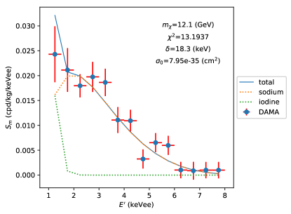
Figure 1: DAMA modulation amplitudes as a function of the measured ionization energy $E^{\prime}$ for the absolute minimum of the pSIDM model in the case of a Maxwellian WIMP velocity distribution. The points with error bars correspond to the combined data of DAMA/NaI Bernabei et al. (1998), DAMA/LIBRA–phase1 Bernabei et al. (2008, 2010) and DAMA/LIBRA–phase2 Bernabei et al. (2018).

The 5–$\sigma$ best-fit DAMA region in the ($m_{\chi}$–$\sigma_{0}$) plane for the pSIDM scenario is compared to the corresponding 90% C.L. upper bounds from other DM searches in Fig. 2 (see Appendix A for some details on how such constraints have been obtained). In the same plot the IDM mass splitting is fixed to the absolute minimum of the $\chi^{2}$, $\delta$=18.3 keV. As can be seen from such figure the DAMA effect is in strong tension with the upper bounds from PICO60, KIMS and PICASSO. On the other hand COSINE-100 Adhikari et al. (2018a), that using the same $NaI$ target of DAMA has recently published an exclusion plot about a factor of two below the DAMA modulation region in the case of an elastic, spin–independent (SI) isoscalar WIMP–nucleon interaction, does not exclude the pSIDM scenario. This is due to the modulation fractions that in the pSIDM model are higher than in the elastic case even for the case of a Maxwellian. In fact inelastic scattering is sensitive to the high–speed tail of the velocity distribution due to the condition $v_{min}\geq v_{min}^{*}$. In particular, the modulation residual measured by DAMA are at the level of $S_{m}^{DAMA}\simeq$ 0.02 events/kg/day/keVee Bernabei et al. (2018), while we estimate a bound from COSINE–100 $S_{0}^{COSINE}\mathrel{\mathop{\kern 0.0pt\hbox to0.0pt{\raise 0.86108pt\hbox{$<$}\hss}}\lower 3.87495pt\hbox{\kern-1.90002pt$\sim$}}$0.13 events/kg/day/keVee after background subtraction (see Appendix A) on the non–modulated component of the signal. This implies $S_{m}^{DAMA}/S_{0}^{DAMA}$ = $S_{m}^{DAMA}/S_{0}^{COSINE}\times S_{0}^{COSINE}/S_{0}^{DAMA}$ $\mathrel{\mathop{\kern 0.0pt\hbox to0.0pt{\raise 0.86108pt\hbox{$>$}\hss}}\lower 3.87495pt\hbox{\kern-1.90002pt$\sim$}}$ 0.12, including a factor $S_{0}^{COSINE}/S_{0}^{DAMA}\simeq$ 0.8 due to a difference between the energy resolutions and efficiencies in the two experiments. For a standard Maxwellian WIMP velocity distribution in the SI elastic case the predicted modulation fractions $S_{m}^{DAMA}/S_{0}^{DAMA}$ are below such bound (for instance, for $m_{\chi}$=10 GeV we find values of $S_{m}^{DAMA}/S_{0}^{DAMA}$ that range between $\simeq$0.05 and $\simeq$0.12 for $E_{ee}<$ 3 keVee). In the pSIDM case, however, the modulation fractions are all above such value. For instance, for $m_{\chi}$=10 GeV and $\delta$=18 keV all the modulation fractions for $E_{ee}<$ 6 keVee (i.e. in the range of the DAMA signal) are above 0.4. This also explains why COSINE–100 does not constrain the pSIDM scenario in the halo–independent approach of the next Section.

We have also performed a combined fit including the upper bounds from such experiments with the addition of COUPP and XENON1T and COSINE–100, finding $\chi_{min}^{2}$=41.1 with a $p$–value 1.5$\times 10^{-3}$ and 18 dof. Including $v_{0}$ and $u_{esc}$ as nuisance parameters in the $\chi^{2}$ (we assume $v_{0}$=(220$\pm$ 20) km/s Koposov et al. (2010) and $u_{esc}$=(550$\pm$ 30) km/s Piffl et al. (2014)) does not improve the fit (we find $\chi_{min}^{2}$=41.0). This confirms that, at variance with the analyses of Ref. Scopel and Yoon (2016); Scopel and Yu (2017), after the release of the DAMA/LIBRA–phase2 data the pSIDM scenario in the Maxwellian case is ruled out. There are two reasons for this. The first reason is that while the DAMA/LIBRA–phase1 data where only sensitive to scattering events off sodium, the DAMA/LIBRA–phase2 data have a lower threshold and are now also sensitive to scattering events off iodine for $E^{\prime}<$2 keVee at low WIMP masses. This makes it more difficult to fit the model to the data since in the pSIDM scenario the scaling between the cross sections off iodine and sodium is fixed (the parameter $c^{n}/c^{p}$, that would allow to change such scaling is locked to the combination that suppresses the response on xenon). Moreover, in the scenario described in Section II a minimal value of the mass splitting parameter $\delta$ is required in order to comply with the condition of Eq.(3), which, at the same time automatically implies that the recoil energy $E^{*}_{R}\equiv E_{R}(v_{min}^{*Na})$, and so a single maximum of the modulation amplitude spectrum, falls inside the range of the DAMA signal Scopel and Yoon (2016) (the energy $E^{*}_{R}$ maximizes the velocity integral in Eq. (15)). Indeed, the DAMA/LIBRA–phase1 data showed a single maximum in the 2.5 keVee$<E^{\prime}<$3 keVee energy bin in the measured modulation amplitudes Bernabei et al. (2008, 2010), implying an acceptable fit for the pSIDM model. On the other hand the DAMA/LIBRA–phase2 data show an energy spectrum of the modulation amplitudes more compatible to a monotonically decreasing one, closer to what expected for elastic scattering. As a consequence of this the DAMA/LIBRA–phase2 $\chi^{2}$ pulls to low values of the $\delta$ mass splitting (indeed, the Maxwellian best–fit configuration $m_{\chi}=12.1~{}{\rm GeV}$, $\delta$=18.3 keV falls below the halo–independent compatibility region discussed in the next Section and shown in Fig. 4), entering in conflict with the requirement of Eq.(3).

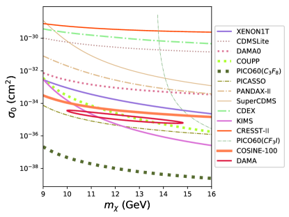
Figure 2: The 5–$\sigma$ best-fit DAMA region for the pSIDM scenario is compared to the corresponding 90% C.L. upper bounds from other DM searches for a Maxwellian WIMP velocity distribution. In the plot the IDM mass splitting is fixed to $\delta$=18.3 keV, which corresponds to the absolute minimum of the $\chi^{2}$.

III.2 Halo–independent analysis

In the halo–independent approach Fox et al. (2011) the expected rate in a direct detection experiment is recast in the form Del Nobile et al. (2013):

$$R_{[E^{\prime}_{1},E^{\prime}_{2}]}(t)=\int_{0}^{\infty}\text{d}\mbox{$v_{min}$}\,\tilde{\eta}(\mbox{$v_{min}$},t)\,\mathcal{R}_{[E^{\prime}_{1},E^{\prime}_{2}]}(\mbox{$v_{min}$})\,,$$ (13)

where the dependence on astrophysics is contained in the halo function:

$$\tilde{\eta}(\mbox{$v_{min}$},t)=\frac{\rho_{\chi}}{m_{\chi}}\,\sigma_{0}\,\eta(\mbox{$v_{min}$},t),$$ (14)

and the WIMP velocity distribution is contained in the velocity integral:

$$\eta(\mbox{$v_{min}$},t)=\int_{\mbox{$v_{min}$}}^{\infty}\text{d}v\,\,\frac{f(v,t)}{v},$$ (15)

while the response function $\mathcal{R}_{[E^{\prime}_{1},E^{\prime}_{2}]}(\mbox{$v_{min}$})$ is given by:

$$\mathcal{R}_{[E^{\prime}_{1},E^{\prime}_{2}]}(\mbox{$v_{min}$})=\sum_{T}N_{T}\frac{v_{T}^{2}}{\sigma_{0}}\frac{d\sigma_{T}}{dE_{R}}\times$$

$$\int_{E^{\prime}_{1}}^{E^{\prime}_{2}}dE^{\prime}\epsilon(E^{\prime}){\cal G}_{T}(E^{\prime},E_{ee}(\mbox{$v_{min}$}).$$ (16)

Notice that for a standard spin–dependent interaction the scattering amplitude in Eq.(6) does not depend on $v_{T}$ so the term $v_{T}^{2}$ in the equation above cancels out in the product $v_{T}^{2}d\sigma_{T}/dE_{R}$.

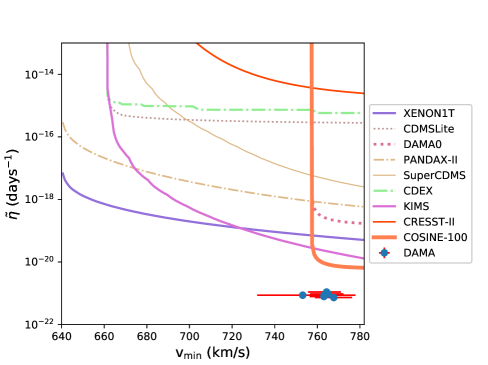
Figure 3: Measurements of $\overline{\tilde{\eta}^{1}}_{[v_{{\rm min},1},v_{{\rm min},2}]}$ (DAMA/LIBRA) and upper bounds $\tilde{\eta}^{\rm lim}$ (same experiments as in Fig. 2) for pSIDM in the benchmark point $m_{\chi}$=11.4 GeV, $\delta$=23.7 keV.

Due to the revolution of the Earth around the Sun, the velocity integral $\tilde{\eta}(\mbox{$v_{min}$},t)$ shows an annual modulation that can be approximated by the first terms of a harmonic series,

$$\tilde{\eta}(\mbox{$v_{min}$},t)=\tilde{\eta}^{0}(\mbox{$v_{min}$})+\tilde{\eta}^{1}(\mbox{$v_{min}$})\,\cos\!\left[\omega(t-t_{0})\right],$$ (17)

with the only requirement that $|\tilde{\eta}^{1}|\leq\tilde{\eta}^{0}$. In this approach measured rates $R^{i}_{[E^{\prime}_{1},E^{\prime}_{2}]}$ (with $i=0,1$) are mapped into suitable averages of the two halo functions $\tilde{\eta}^{i}$. Averages $\overline{\tilde{\eta}^{i}}_{[v_{{\rm min},1},v_{{\rm min},2}]}$ ($i=0,1$) using $\mathcal{R}(\mbox{$v_{min}$})$ in Eq. (16) as a weight function can then be directly obtained from the experimental data $R^{i}_{[E^{\prime}_{1},E^{\prime}_{2}]}$ as Del Nobile et al. (2013):

$$\overline{\tilde{\eta}^{i}}_{[v_{{\rm min},1},v_{{\rm min},2}]} = \frac{\int_{0}^{\infty}\text{d}\mbox{$v_{min}$}\,\tilde{\eta}^{i}(\mbox{$v_{min}$})\,\mathcal{R}_{[E^{\prime}_{1},E^{\prime}_{2}]}(\mbox{$v_{min}$})}{\int_{0}^{\infty}\text{d}\mbox{$v_{min}$}\,\mathcal{R}_{[E^{\prime}_{1},E^{\prime}_{2}]}(\mbox{$v_{min}$})}=$$ (18)

$$= \frac{R^{i}_{[E^{\prime}_{1},E^{\prime}_{2}]}}{\int_{0}^{\infty}\text{d}\mbox{$v_{min}$}\,\mathcal{R}_{[E^{\prime}_{1},E^{\prime}_{2}]}(\mbox{$v_{min}$})},$$

The result of such procedure is shown in Fig. 3, where the determinations of $\overline{\tilde{\eta}^{1}}_{[v_{{\rm min},1},v_{{\rm min},2}]}$ from DAMA/LIBRA–phase2 data are shown with error bars for the benchmark point $m_{\chi}$=11.4 GeV, $\delta$=23.7 keV.

The velocity intervals $[v_{{\rm min},1},v_{{\rm min},2}]$ are defined as those velocity intervals where the weight function $\mathcal{R}_{[E^{\prime}_{1},E^{\prime}_{2}]}(\mbox{$v_{min}$})$ is sizeably different from zero. In particular, to determine the $v_{min}$ interval corresponding to each detected energy interval $[E^{\prime}_{1},E^{\prime}_{2}]$ in DAMA we choose to use $68\%$ central quantile intervals of the response function, i.e. we determine ${\mbox{$v_{min}$}}_{,1}$ and ${\mbox{$v_{min}$}}_{,2}$ such that the areas under the function $\mathcal{R}_{[E^{\prime}_{1},E^{\prime}_{2}]}(\mbox{$v_{min}$})$ to the left of ${\mbox{$v_{min}$}}_{,1}$ and to the right of ${\mbox{$v_{min}$}}_{,2}$ are each separately $16\%$ of the total area under the function. This gives the horizontal width of the crosses corresponding to the rate measurements in Fig. 3. On the other hand, the horizontal placement of the vertical bar in the crosses corresponds to the average of $v_{min}$, i.e., $\mbox{$v_{min}$}(\text{vertical bar})=\big{[}\int_{0}^{\infty}\text{d}\mbox{$v_{min}$}\,\mbox{$v_{min}$}\mathcal{R}_{[E^{\prime}_{1},E^{\prime}_{2}]}(\mbox{$v_{min}$})\big{]}/\big{[}\int_{0}^{\infty}\text{d}\mbox{$v_{min}$}\,\mathcal{R}_{[E^{\prime}_{1},E^{\prime}_{2}]}(\mbox{$v_{min}$})\big{]}$. The extension of the vertical bar shows the $1\sigma$ interval around the central value of the measured rate.

To compute upper bounds on $\tilde{\eta}^{\,0}$ from upper limits $R_{[E^{\prime}_{1},E^{\prime}_{2}]}^{\rm lim}$ on the unmodulated rates, we follow the conservative procedure in Ref. Fox et al. (2011). Since $\tilde{\eta}^{\,0}(\mbox{$v_{min}$})$ is by definition a non-decreasing function, the lowest possible $\tilde{\eta}^{0}(\mbox{$v_{min}$})$ function passing through a point $(v_{0},\tilde{\eta}^{\,0})$ in $v_{min}$ space is the downward step function $\tilde{\eta}^{0}\,\theta(v_{0}-\mbox{$v_{min}$})$. The maximum value of $\tilde{\eta}^{0}$ allowed by a null experiment at a certain confidence level, denoted by $\tilde{\eta}^{\rm lim}(v_{0})$, is then determined by the experimental limit on the rate $R_{[E^{\prime}_{1},E^{\prime}_{2}]}^{\rm lim}$ as

$$\tilde{\eta}^{\rm lim}(v_{0})=\frac{R^{\rm lim}_{[E^{\prime}_{1},E^{\prime}_{2}]}}{\int_{0}^{v_{0}}\text{d}\mbox{$v_{min}$}\,\mathcal{R}_{[E^{\prime}_{1},E^{\prime}_{2}]}(\mbox{$v_{min}$})}\ .$$ (19)

The corresponding upper limits at 90% C.L. are shown as continuous lines in Figs. 3 for the same experiments shown in Fig. 2.

For the specific benchmark $m_{\chi}$=11.4 GeV, $\delta$=23.7 keV shown in Fig. 3 one can see that pSIDM cannot be ruled out as an explanation of the DAMA/LIBRA effect since in all the energy range of the signal one has $|\overline{\tilde{\eta}^{1}}_{[v_{{\rm min},1},v_{{\rm min},2}]}|\ll\tilde{\eta}^{\rm lim}$. The same benchmark is represented by a starred point in Fig 4 and lies inside the the closed contour where the compatibility factor defined as Scopel and Yoon (2016):

$${\cal D}(m_{DM},\delta)\equiv\max_{i}\left(\frac{\overline{\tilde{\eta}^{1}}_{[v^{i}_{{\rm min},1},v^{i}_{{\rm min},2}]}-\sigma_{i}}{\min_{i}\tilde{\eta}^{\rm lim}(v_{0}^{i})}\right),$$ (20)

is less than unity. In the equation above $[v^{i}_{{\rm min},1},v^{i}_{{\rm min},2}]$ and $v_{0}^{i}$ represent intervals and averages of $v_{min}$ for each of the $i$=1…14 DAMA/LIBRA bins below $E^{\prime}$=8 keVee, while $\sigma_{i}$ is the 1–$\sigma$ fluctuation on $\overline{\tilde{\eta}^{1}}_{[v^{i}_{{\rm min},1},v^{i}_{{\rm min},2}]}$. In particular, the requirement ${\cal D}(m_{DM},\delta)<$1 ensures that within the solid closed contour of Fig. 4 no 1–$\sigma$ interval of the quantities $\overline{\tilde{\eta}^{1}}_{[v_{{\rm min},1},v_{{\rm min},2}]}$ obtained from the DAMA/LIBRA data lies completely above any of the upper bounds $\tilde{\eta}^{\rm lim}$. In Fig. 4 we also provide additional dashed closed contours which correspond to an alternative, more accurate definition of the compatibility factor: once the averages of the modulated halo function $\overline{\tilde{\eta}^{1}}$ are determined from the DAMA data, we determine a minimal set of averages of the unmodulated halo function $\overline{\tilde{\eta}^{0}}$ complying with the condition that $\overline{\tilde{\eta}^{0}}$ is a non–increasing function of $v_{min}$ and that $|\overline{\tilde{\eta}^{1}}|<\xi\overline{\tilde{\eta}^{0}}$ with $\xi\leq$1 ($\xi$=1 corresponding to 100% modulation). We then use the $\overline{\tilde{\eta}^{0}}$’s to calculate for different values of $\xi$ the expected rate $R^{exp}_{n}(m_{DM},\delta,\xi)$ for each experiment exp and energy bin $n$. Indicating with $R^{exp,lim}_{n}$ the corresponding 90% C.L. upper bound we adopt as compatibility factor:

$${\cal D}^{\prime}(m_{DM},\delta,\xi)\equiv\max_{exp,n}\frac{R^{exp}_{n}(m_{DM},\delta,\xi)}{R^{exp,lim}_{n}},$$ (21)

where, again, ${\cal D}^{\prime}<$1 indicates compatibility. As long as $\xi=1$, ${\cal D}$ and ${\cal D}^{\prime}$ yield similar results (implying that, although the DAMA result requires all the $\overline{\tilde{\eta}^{1}}$’s the bound is driven by only one of the corresponding $\overline{\tilde{\eta}^{0}}$’s). In particular, from Fig. 4 one can see that in a halo–independent approach the pSIDM scenario can explain the DAMA/LIBRA data for 7 GeV $\mathrel{\mathop{\kern 0.0pt\hbox to0.0pt{\raise 0.86108pt\hbox{$<$}\hss}}\lower 3.87495pt\hbox{\kern-1.90002pt$\sim$}}m_{\chi}\mathrel{\mathop{\kern 0.0pt\hbox to0.0pt{\raise 0.86108pt\hbox{$<$}\hss}}\lower 3.87495pt\hbox{\kern-1.90002pt$\sim$}}$ 17 GeV and 18 keV$\mathrel{\mathop{\kern 0.0pt\hbox to0.0pt{\raise 0.86108pt\hbox{$<$}\hss}}\lower 3.87495pt\hbox{\kern-1.90002pt$\sim$}}\delta\mathrel{\mathop{\kern 0.0pt\hbox to0.0pt{\raise 0.86108pt\hbox{$<$}\hss}}\lower 3.87495pt\hbox{\kern-1.90002pt$\sim$}}$29 keV. As expected, when $\xi<1$ (smaller modulation fractions) the compatibility region in Fig. 4 shrinks. Inside the smallest dashed contour of Fig. 4 ${\cal D}^{\prime}$ eventually reaches a plateau with minimum value slightly lower than 0.1, implying the compatibility of modulation fractions as low as $\simeq$0.1.

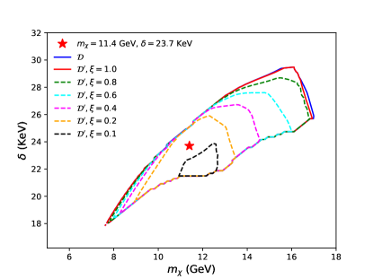
Figure 4: In the region inside the closed solid contour the compatibility parameter ${\cal D}$ defined in Eq. (20) is less than unity, implying that no 1–$\sigma$ interval of the quantities $\overline{\tilde{\eta}^{1}}_{[v_{{\rm min},1},v_{{\rm min},2}]}$ obtained from the DAMA/LIBRA data lies completely above any of the upper bounds $\tilde{\eta}^{\rm lim}$. Inside the dashed closed contours the alternative compatibility factor ${\cal D}^{\prime}$ defined in Eq. (21) is less than unity for different values of the maximal modulation fraction $\xi$. The starred point corresponds to the benchmark shown in Fig. 3.

IV Conclusions

We have shown that the Weakly Interacting Massive Particle scenario of proton-philic spin-dependent inelastic Dark Matter (pSIDM) can still provide a viable explanation of the observed DAMA modulation amplitude in compliance with the constraints from other experiments after the release of the DAMA/LIBRA phase–2 data. The pSIDM scenario provided a viable explanation of DAMA/LIBRA–phase 1 both for a Maxwellian WIMP velocity distribution and in a halo–independent approach. At variance with DAMA/LIBRA–phase1, for which the modulation amplitudes showed an isolated maximum at low energy, the DAMA/LIBRA–phase2 spectrum is compatible to a monotonically decreasing one. Moreover, due to its lower threshold, it is sensitive to WIMP–iodine interactions at low WIMP masses. Due to the combination of these two effects pSIDM can now explain the modulation observed by DAMA/LIBRA only when the WIMP velocity distribution departs from a standard Maxwellian. In this case the WIMP mass $m_{\chi}$ and mass splitting $\delta$ fall in the approximate ranges 7 GeV $\mathrel{\mathop{\kern 0.0pt\hbox to0.0pt{\raise 0.86108pt\hbox{$<$}\hss}}\lower 3.87495pt\hbox{\kern-1.90002pt$\sim$}}m_{\chi}\mathrel{\mathop{\kern 0.0pt\hbox to0.0pt{\raise 0.86108pt\hbox{$<$}\hss}}\lower 3.87495pt\hbox{\kern-1.90002pt$\sim$}}$ 17 GeV and 18 keV$\mathrel{\mathop{\kern 0.0pt\hbox to0.0pt{\raise 0.86108pt\hbox{$<$}\hss}}\lower 3.87495pt\hbox{\kern-1.90002pt$\sim$}}\delta\mathrel{\mathop{\kern 0.0pt\hbox to0.0pt{\raise 0.86108pt\hbox{$<$}\hss}}\lower 3.87495pt\hbox{\kern-1.90002pt$\sim$}}$29 keV. The recent COSINE–100 bound is naturally evaded in the pSDIM scenario due to its large expected modulation fractions, because inelastic scattering is sensitive to the high–speed tail of the velocity distribution.

We conclude by pointing out that strictly speaking our analysis can only lead to the conclusion that in the pSIDM scenario it is not possible to rule out a DAMA explanation in terms of WIMPs in a halo-independent way. On the other hand, the problem of inverting the halo function $\tilde{\eta}^{1}$ to obtain a velocity distribution $f(v)$ that, due to the boost from the Galactic to the lab rest frames, leads to the correct time and energy dependence of the DAMA signal is a complex and highly degenerate one that would require a dedicated analysis beyond the scope of our paper. Moreover, due to the very strong existing limits from null searches the pSIDM scenario requires considerable tuning, such as a large suppression of the spin–independent coupling, a specific range of the Galactic escape velocity according to Eq. (3) and the tuning of the $c^{n}/c^{p}$ couplings ratio. As a consequence pSIDM appears challenging both from the point of view of particle physics model–building and of that of astrophysics. However, in spite of these challenges, at the very least the pSIDM scenario can be considered as a proof of concept of the fact that the parameter space of WIMP direct detection is wider than usually assumed and that experimentally an explanation of the DAMA signal in terms of WIMPs has not yet been completely probed.

Appendix A Experiments

With the exception of the recent COSINE-100 result Adhikari et al. (2018a) we fix the experimental input (exposure, energy resolution, quenching factors, efficiency, measured count rates, etc.) for both the DAMA/LIBRA experiment and for other DM searches as described in appendix B of Kang et al. (2018b) and appendix A of Kang et al. (2018c). Recently Adhikari et al. (2018a) the COSINE–100 collaboration has published a bound about a factor of two below the DAMA region using 106 kg of $NaI$, the same target of DAMA. Such result assumes an elastic, spin–dependent isoscalar WIMP nucleus interaction for a WIMP Maxwellian velocity distribution with standard parameters, and relies on a Montecarlo Adhikari et al. (2018b) to subtract the different backgrounds of each of the eight crystals used in the analysis. In Ref. Adhikari et al. (2018a) the amount of residual background after subtraction is not provided, and depends on the expected signal shape, so should not in principle be used to constrain a signal with a spectral shape different from the specific scenario adopted in Ref. Adhikari et al. (2018a). However, especially in the halo–independent case, for which the expected spectral shape cannot be used to constrain the background, we deem that using the same residual background of Ref. Adhikari et al. (2018a) should lead to an optimistic estimate of the bound. So we have assumed for COSINE–100 a constant background $b$ at low energy (2 keVee$<E_{ee}<$ 8 keVee), and we have estimated $b$ by tuning it to reproduce the exclusion plot in Fig.4 of Ref. Adhikari et al. (2018a) for the isoscalar spin-independent elastic case. The result of our procedure yields $b\simeq$0.13 events/kg/day/keVee, which implies a subtraction of about 95% of the background. We have then used the same value to calculate the bounds for pSIDM. We take the energy resolution $\sigma/\mbox{keV}=0.3171\sqrt{E_{ee}/\mbox{keVee}}+0.008189E_{ee}/\mbox{keVee}$ averaged over the COSINE–100 crystals cos and the efficiency for nuclear recoils from Fig.1 of Ref. Adhikari et al. (2018a). Quenching factors for sodium and iodine are assumed to be equal to 0.3 and 0.09 respectively, the same values used by DAMA.

References

- (1)
- Ade et al. (2014) P. A. R. Ade et al. (Planck), Astron. Astrophys. 571, A16 (2014), eprint 1303.5076.
- Drukier et al. (1986) A. K. Drukier, K. Freese, and D. N. Spergel, Phys. Rev. D33, 3495 (1986).
- Bernabei et al. (2008) R. Bernabei et al. (DAMA), Eur. Phys. J. C56, 333 (2008), eprint 0804.2741.
- Bernabei et al. (2010) R. Bernabei et al. (DAMA, LIBRA), Eur. Phys. J. C67, 39 (2010), eprint 1002.1028.
- Bernabei et al. (2013) R. Bernabei et al., Eur. Phys. J. C73, 2648 (2013), eprint 1308.5109.
- Scopel and Yoon (2016) S. Scopel and K.-H. Yoon, JCAP 1602, 050 (2016), eprint 1512.00593.
- Scopel and Yu (2017) S. Scopel and H. Yu, JCAP 1704, 031 (2017), eprint 1701.02215.
- Bernabei et al. (2018) R. Bernabei et al. (2018), eprint 1805.10486.
- Kahlhoefer et al. (2018) F. Kahlhoefer, F. Reindl, K. Sch ffner, K. Schmidt-Hoberg, and S. Wild, JCAP 1805, 074 (2018), eprint 1802.10175.
- Baum et al. (2018) S. Baum, K. Freese, and C. Kelso (2018), eprint 1804.01231.
- Kang et al. (2018a) S. Kang, S. Scopel, G. Tomar, and J.-H. Yoon, JCAP 1807, 016 (2018a), eprint 1804.07528.
- Herrero-Garcia et al. (2018) J. Herrero-Garcia, A. Scaffidi, M. White, and A. G. Williams (2018), eprint 1804.08437.
- Adhikari et al. (2018a) G. Adhikari et al., Nature 564, 83 (2018a).
- Aprile et al. (2018) E. Aprile et al. (XENON) (2018), eprint 1805.12562.
- Cui et al. (2017) X. Cui et al. (PandaX-II), Phys. Rev. Lett. 119, 181302 (2017), eprint 1708.06917.
- Akerib et al. (2016) D. S. Akerib et al. (2016), eprint 1608.07648.
- Ahmed et al. (2011) Z. Ahmed et al. (CDMS-II), Phys. Rev. Lett. 106, 131302 (2011), eprint 1011.2482.
- Agnese et al. (2014a) R. Agnese et al. (SuperCDMS), Phys. Rev. Lett. 112, 041302 (2014a), eprint 1309.3259.
- Agnese et al. (2014b) R. Agnese et al. (SuperCDMS), Phys. Rev. Lett. 112, 241302 (2014b), eprint 1402.7137.
- Agnese et al. (2015) R. Agnese et al. (SuperCDMS), Phys. Rev. D92, 072003 (2015), eprint 1504.05871.
- Ullio et al. (2001) P. Ullio, M. Kamionkowski, and P. Vogel, JHEP 07, 044 (2001), eprint hep-ph/0010036.
- Del Nobile et al. (2015) E. Del Nobile, G. B. Gelmini, A. Georgescu, and J.-H. Huh, JCAP 1508, 046 (2015), eprint 1502.07682.
- Anand et al. (2014) N. Anand, A. L. Fitzpatrick, and W. C. Haxton, Phys. Rev. C89, 065501 (2014), eprint 1308.6288.
- Behnke et al. (2012) E. Behnke et al. (COUPP), Phys. Rev. D86, 052001 (2012), [Erratum: Phys. Rev.D90,no.7,079902(2014)], eprint 1204.3094.
- Behnke et al. (2017) E. Behnke et al., Astropart. Phys. 90, 85 (2017), eprint 1611.01499.
- Amole et al. (2017) C. Amole et al. (PICO), Phys. Rev. Lett. 118, 251301 (2017), eprint 1702.07666.
- Amole et al. (2015) C. Amole et al. (PICO), Phys. Rev. Lett. 114, 231302 (2015), eprint 1503.00008.
- Tucker-Smith and Weiner (2001) D. Tucker-Smith and N. Weiner, Phys. Rev. D64, 043502 (2001), eprint hep-ph/0101138.
- Kang et al. (2018b) S. Kang, S. Scopel, G. Tomar, and J.-H. Yoon (2018b), eprint 1805.06113.
- Koposov et al. (2010) S. E. Koposov, H.-W. Rix, and D. W. Hogg, Astrophys. J. 712, 260 (2010), eprint 0907.1085.
- Piffl et al. (2014) T. Piffl et al., Astron. Astrophys. 562, A91 (2014), eprint 1309.4293.
- Bernabei et al. (1998) R. Bernabei et al., Phys. Lett. B424, 195 (1998).
- Fox et al. (2011) P. J. Fox, J. Liu, and N. Weiner, Phys. Rev. D83, 103514 (2011), eprint 1011.1915.
- Del Nobile et al. (2013) E. Del Nobile, G. Gelmini, P. Gondolo, and J.-H. Huh, JCAP 1310, 048 (2013), eprint 1306.5273.
- Kang et al. (2018c) S. Kang, S. Scopel, G. Tomar, J.-H. Yoon, and P. Gondolo (2018c), eprint 1808.04112.
- Adhikari et al. (2018b) P. Adhikari et al. (COSINE-100), Eur. Phys. J. C78, 490 (2018b), eprint 1804.05167.
- (38) COSINE–100 Collaboration, private communication.