Online learning with feedback graphs
and switching costs

Abstract

We study online learning when partial feedback information is provided following every action of the learning process, and the learner incurs switching costs for changing his actions. In this setting, the feedback information system can be represented by a graph, and previous works studied the expected regret of the learner in the case of a clique (Expert setup), or disconnected single loops (Multi-Armed Bandits (MAB)). This work provides a lower bound on the expected regret in the Partial Information (PI) setting, namely for general feedback graphs –excluding the clique. Additionally, it shows that all algorithms that are optimal without switching costs are necessarily sub-optimal in the presence of switching costs, which motivates the need to design new algorithms. We propose two new algorithms: Threshold Based EXP3 and EXP3.SC. For the two special cases of symmetric PI setting and MAB, the expected regret of both of these algorithms is order optimal in the duration of the learning process. Additionally, Threshold Based EXP3 is order optimal in the switching cost, whereas EXP3.SC is not. Finally, empirical evaluations show that Threshold Based EXP3 outperforms the previously proposed order-optimal algorithms EXP3 SET in the presence of switching costs, and Batch EXP3 in the MAB setting with switching costs.

1 Introduction

Online learning has a wide variety of applications like classification, estimation, and ranking, and it has been investigated in different areas, including learning theory, control theory, operations research, and statistics. The problem can be viewed as a one player game against an adversary. The game runs for $T$ rounds and at each round the player chooses an action from a given set of $K$ actions. Every action $k\in[K]$ performed at round $t\in[T]$ carries a loss, that is a real number in the interval $[0,1]$. The losses for all pairs $(k,t)$ are assigned by the adversary before the game starts. The player also incurs a fixed and known Switching Cost (SC) every time he changes his action, that is an arbitrary real number $c>0$. The expected regret is the expectation of the sum of losses associated to the actions performed by the player plus the SCs minus the losses incurred by the best fixed action in hindsight. The goal of the player is to minimize the expected regret over the duration of the game.

Based on the feedback information received after each action, online learning can be divided into three categories: Multi-Armed Bandit (MAB), Partial Information (PI), and Expert setting. In a MAB setting, at any given round the player only incurs the loss corresponding to the selected action, which implies the player only observes the loss of the selected action. In a PI setting, the player incurs the loss of the selected action $k\in[K]$, as well as observes the losses that he would have incurred in that round by taking actions in a subset of $[K]\backslash\{k\}$. This feedback system can be viewed as a time-varying directed graph $G_{t}$ with $K$ nodes, where a directed edge $k\to j$ in $G_{t}$ indicates that performing an action $k$ at round $t$ also reveals the loss that the player would have incurred if action $j$ was taken at round $t$. In an Expert setting, taking an action reveals the losses that the player would have incurred by taking any of the other actions in that round. In this extremal case, the feedback system $G_{t}$ corresponds to a time-invariant, undirected clique.

Online learning with PI has been used to design a variety of systems Gentile and Orabona, (2014); Katariya et al., (2016); Zong et al., (2016); Rangi et al., 2018c . In these applications, feedback captures the idea of side information provided to the player during the learning process. For example, the performance of an employee can provide information about the performance of other employees with similar skills, or the rating of a web page can provide information on ratings of web pages with similar content. In most of these applications, switching between the actions is not free. For example, a company incurs a cost associated to the learning phase while shifting an employee among different tasks, or switching the content of a web page frequently can exasperate users and force them to avoid visiting it. Similarly, re-configuring the production line in a factory is a costly process, and changing the stock allocation in an investment portfolio is subject to certain fees. Despite the many applications where both SC and PI are an integral part of the learning process, the study of online learning with SC has been limited only to the MAB and Expert settings. In the MAB setting, it has been shown that the expected regret of any player is at least $\tilde{\Omega}(c^{1/3}K^{1/3}T^{2/3})$ Dekel et al., (2014), and that Batch EXP3 is an order optimal algorithm Arora et al., (2012). In the Expert setting, it has been shown that the expected regret is at least $\tilde{\Omega}(\sqrt{\log(K)T})$ Cesa-Bianchi and Lugosi, (2006), and order optimal algorithms have been proposed in Geulen et al., (2010); Gyorgy and Neu, (2014). The PI setup has been investigated only in the absence of SC, and for any fixed feedback system $G_{t}=G$ with independence number $\alpha(G)>1$, it has been shown that the expected regret is at least $\tilde{\Omega}(\sqrt{\alpha(G)T})$ Mannor and Shamir, (2011).

Scenarios	Threshold based EXP3	EXP3.SC	Lower Bound
For all $t$, $G_{t}=G$	$\tilde{O}(c^{1/3}(\mbox{mas}(G))^{1/3}T^{2/3})$	$\tilde{O}(c^{4/3}(\mbox{mas}(G))^{2/3}T^{2/3})$	$\tilde{\Omega}(c^{1/3}\alpha(G)^{1/3}T^{2/3})$
Symmetric PI	$\tilde{O}(c^{1/3}\alpha(G)^{1/3}T^{2/3})$	$\tilde{O}(c^{4/3}\alpha(G)^{2/3}T^{2/3})$	$\tilde{\Omega}(c^{1/3}\alpha(G)^{1/3}T^{2/3})$
MAB	$\tilde{O}(c^{1/3}K^{1/3}T^{2/3})$	$\tilde{O}(c^{4/3}K^{2/3}T^{2/3})$	$\tilde{\Omega}(c^{1/3}K^{1/3}T^{2/3})$
$G_{1:T}$	$\tilde{O}(c\sum_{t=1}^{t^{*}}{\mbox{mas}(G_{(t)})/\mbox{mas}(G_{(T)})})$	$\tilde{O}(\sum_{t=1}^{n^{*}}{\mbox{mas}(G_{(t)})/\mbox{mas}(G_{(T)})})$	$\tilde{\Omega}(c^{1/3}\beta(G_{1:T})^{1/3}T^{2/3})$
Equi-informational	$\tilde{O}(c^{1/3}\alpha(G_{1})^{1/3}T^{2/3})$	$\tilde{O}(c^{4/3}\alpha(G_{1})^{2/3}T^{2/3})$	$\tilde{\Omega}(c^{1/3}\beta(G_{1:T})^{1/3}T^{2/3})$

Table 1: Comparison of Threshold based EXP3 and EXP3.SC.

1.1 Contributions

We provide a lower bound on the expected regret for any sequence of feedback graphs $G_{1},\ldots G_{T}$ in the PI setting with SC. We show that for any sequence of feedback graphs $G_{1:T}=\{G_{1},\ldots G_{T}\}$ with independence sequence number $\beta(G_{1:T})>1$, the expected regret of any player is at least $\tilde{\Omega}(c^{1/3}\beta(G_{1:T})^{1/3}T^{2/3})$. We then show that for $G_{1:T}$ with $\alpha(G_{t})>1$ for all $t\leq T$, the expected regret of any player is at least $\tilde{\Omega}(c^{1/3}\sum_{G_{j}\in\mathcal{G}}\alpha(G_{j})^{1/3}N(G_{j})^{2/3})$, where $\mathcal{G}$ is the set of unique feedback graphs in the sequence $G_{1:T}$, and $N(G_{j})=\sum_{t=1}^{T}\mathbf{1}(G_{t}=G_{j})$ is the number of rounds for which the feedback graph $G_{j}$ is seen in $T$ rounds. These results introduce a new figure of merit $\beta(G_{1:T})$ in the PI setting, which can also be used to generalize the lower bound given in the PI setting without SC  Mannor and Shamir, (2011). A consequence of these results is that the presence of SC changes the asymptotic regret by at least a factor $T^{1/6}$. Additionally, these results also recover the lower bound on the expected regret in the MAB setting Dekel et al., (2014).

We also show that in the PI setting for any algorithm that is order optimal without SC, there exists an assignment of losses from the adversary that forces the algorithm to make at least $\tilde{\Omega}(T)$ switches, thus increasing its asymptotic regret by at least a factor $T^{1/2}$. This shows that any algorithm that is order optimal in the PI setting without SC, is necessarily sub-optimal in the presence of SC, and motivates the development of new algorithms in the PI setting and in the presence of SC.

We propose two new algorithms for the PI setting with SC: Threshold-Based EXP3 and EXP3.SC. Threshold-Based EXP3 requires the knowledge of $T$ in advance, whereas EXP3.SC does not. The performance of these algorithms is given for different scenarios in Table 1. The algorithms are order optimal in $T$ and $\beta(G_{1:T})$ for two special cases of feedback information system: symmetric PI setting i.e. the feedback graph $G_{t}=G$ is fixed and un-directed, and MAB. In these two cases, $\beta(G_{1:T})$ equals $\alpha(G)$ and $K$ respectively. The state-of-art algorithm EXP3 SET in PI setting without SC is known to be order optimal only for these cases as well Alon et al., (2017). Threshold Based EXP3 is order optimal in the SC $c$ as well, while EXP3.SC has an additional factor of $c$ in its expected regret. In the time-varying case, for sequence $G_{1:T}$, the expected regret is dependent on the worst $t^{*}$ and $n^{*}$ instances of the ratio of $\mbox{mas}(G_{t})$ and $\mbox{mas}(G_{(T)})$, where $\{\mbox{mas}(G_{(1)}),\mbox{mas}(G_{(2)}),\ldots,\mbox{mas}(G_{(T)})\}$ are the sizes of the maximal acyclic subgraphs of $G_{1:T}$ arranged in non-increasing order, $t^{*}={\lceil T^{2/3}c^{-2/3}\mbox{mas}^{1/3}(G_{(T)})\rceil}$ and $n^{*}=0.5\mbox{mas}^{1/3}(G_{(T)})T^{2/3}c^{1/3}$. Finally, Table 1 also provides the performance in the equi-informational setting, namely when $G_{t}$ is undirected and all the maximal acyclic subgraphs in $G_{1:T}$ have the same size. The proofs of all these results are available online Rangi and Franceschetti, 2018b .

Numerical comparison shows that Threshold Based EXP3 outperforms EXP3 SET in the presence of SCs. Threshold Based EXP3 also outperforms Batch EXP3, which is another order optimal algorithm for the MAB setting with SC Arora et al., (2012).

1.2 Related Work

In the absence of SC, the lower bound on the expected regret is known for all three categories of online learning problems. In the MAB setting, the expected regret is at least $\tilde{\Omega}(\sqrt{KT})$ Auer et al., (2002); Cesa-Bianchi and Lugosi, (2006); Rangi et al., 2018d . In the PI setting with fixed feedback graph $G$, the expected regret is at least $\tilde{\Omega}(\sqrt{\alpha(G)T})$ Mannor and Shamir, (2011). In the Expert setting, the expected regret is at least $\tilde{\Omega}(\sqrt{\log(K)T})$ Cesa-Bianchi and Lugosi, (2006). All three cases present an asymptotic regret factor $T^{1/2}$. In contrast, in the presence of SC the expected regrets for MAB and Expert settings present different factors, namely $T^{2/3}$ and $T^{1/2}$ respectively. The expected regret is at least $\tilde{\Omega}(c^{1/3}K^{1/3}T^{2/3})$ in the MAB setting and $\tilde{\Omega}(\sqrt{\log(K)T})$ in the Expert setting Dekel et al., (2014). This work provides the lower bound on the expected regret $\tilde{\Omega}(c^{1/3}\beta(G_{1:T})^{1/3}T^{2/3})$ for the PI setting in the presence of SC. For the case without SC, this work establishes that the lower bound in PI setting is $\tilde{\Omega}(\sqrt{\beta(G_{1:T})T})$.

The PI setting was first considered in Alon et al., (2013); Mannor and Shamir, (2011), and many of its variations have been studied without SC Alon et al., (2015, 2013); Caron et al., (2012); Rangi et al., 2018b ; Langford and Zhang, (2008); Kocák et al., (2016); Rangi et al., 2018a ; Wu et al., (2015); Rangi and Franceschetti, 2018a . In the adversarial setting we described, all of these algorithms are order optimal in the MAB and symmetric PI settings, but they also require the player to have knowledge of the graph $G_{t}$ before performing an action. The algorithm EXP3 SET does not require such knowledge Alon et al., (2017). We show that all of these algorithms are sub-optimal in the PI setting with SC, and propose new algorithms that are order optimal in the MAB and symmetric PI settings.

In the expert setting with SC, there are two order optimal algorithms with expected regret $\tilde{O}(\sqrt{\log(K)T})$ Geulen et al., (2010); Gyorgy and Neu, (2014). In the MAB setting with SC, Batch EXP3 is an order optimal algorithm with expected regret $\tilde{O}(c^{1/3}K^{1/3}T^{2/3})$ Arora et al., (2012). This algorithm has also been used to solve a variant of the MAB setting Feldman et al., (2016). In the MAB setting, our algorithm has the same order of expected regret as Batch EXP3 but it numerically outperforms Batch EXP3.

There is a large literature on a continuous variation of the MAB setting, where the number of actions $K$ depends on the number of rounds $T$. In this setting, the case without the SC was investigated in Auer et al., (2007); Bubeck et al., (2011); Kleinberg, (2005); Yu and Mannor, (2011). Recently, the case including SC has also been studied in Koren et al., 2017a ; Koren et al., 2017b . In Koren et al., 2017a , the algorithm Slowly Moving Bandits (SMB) has been proposed and in Koren et al., 2017b , it has been extended to different settings. These algorithms incur an expected regret linear in $T$ when applied in our discrete setting.

2 Problem Formulation

Before the game starts, the adversary fixes a loss sequence $\ell_{1},\ldots,\ell_{T}\in[0,1]^{K}$, assigning a loss in $[0,1]$ to $K$ actions for $T$ rounds. At round $t$, the player performs an action $i_{t}\in[K]$, and incurs the loss $\ell_{t}(i_{t})$ assigned by the adversary. If $i_{t}\neq i_{t-1}$, then the player also incurs a cost $c>0$ in addition to the loss $\ell_{t}(i_{t})$.

In the PI setting, the feedback system can be viewed as a time-varying directed graph $G_{t}$ with $K$ nodes, where a directed edge $k\to j$ indicates that choosing action $k$ at round $t$ also reveals the loss that the player would have incurred if action $j$ were taken at round $t$. Let $S_{t}(i)=\{j:i\to j\mbox{ is a directed edge in }G_{t}\}$. Following the action $i_{t}$, the player observes the losses he would have incurred in round $t$ by performing actions in the subset $S_{t}(i_{t})\subseteq[K]$. Since the player always observes its own loss, $i_{t}\in S_{t}(i_{t})$. In a MAB setup, the feedback graph $G_{t}$ has only self loops, i.e. for all $t\leq T$ and $i\in[K]$, $S_{t}(i)=\{i\}$. In an Expert setup, $G_{t}$ is a undirected clique i.e. for all $t\leq T$ and $i\in[K]$, $S_{t}(i)=[K]$ . The expected regret of a player’s strategy $\delta$ is defined as

$$\begin{split}R^{\delta}(\ell_{1:T},c)&=\mathbf{E}\left[\sum_{t=1}^{T}\ell_{t}(i_{t})+\sum_{t=2}^{T}c\cdot\textbf{1}(i_{t-1}\neq i_{t})\right]\\ &\qquad-\min_{k\in[K]}\sum_{t=1}^{T}\ell_{t}(k).\end{split}$$ (1)

In words, the expected regret is the expectation of the sum of losses associated to the actions performed by the player plus the SCs minus the losses incurred by the best fixed action in the hindsight, and the objective of the player is to minimize the expected regret.

3 Lower Bound in PI setting with SC

We start by defining the independence sequence number for a sequence of graphs $G_{1:T}$.

Definition 3.1.

Given $G_{1:T}$, let $P(G_{t})$ be the set of all the possible independent sets of the graph $G_{t}$. The independence sequence number $\beta(G_{1:T})$ is the largest cardinality among all intersections of the independent sets $s_{1}\cap s_{2}\cap\ldots\cap s_{T}$, where $s_{t}\in P(G_{t})$. Namely,

$${\beta(G_{1:T})}=\max_{s_{1}\in P(G_{1}),\ldots s_{T}\in P(G_{T})}\lvert s_{1}\cap s_{2}\cap\ldots\cap s_{T}\rvert.$$ (2)

Definition 3.2.

The independence sequence set $\mathcal{I}(G_{1:T})$ is the set $s_{1}\cap s_{2}\cap\ldots s_{T}$ attaining the maximum in (2).

We use the notion of $\beta(G_{1:T})$ to provide a lower bound on the expected regret in the PI setting with SC.

Theorem 1.

For any $G_{1:T}$ with $\beta(G_{1:T})>1$, there exists a constant $b>0$ and an adversary’s strategy (Algorithm 1) such that for all $T\geq 27c\log_{2}^{3/2}(T)/\beta(G_{1:T})^{2}$, and for any player’s strategy $\mathcal{A}$, the expected regret of $\mathcal{A}$ is at least $b\,c^{1/3}\beta(G_{1:T})^{1/3}T^{2/3}/\log T$.

The proof of Theorem 1 relies on Yao’s minimax principle Yao, (1977). A randomized adversary strategy is constructed such that the expected regret of a player, whose action at any round is a deterministic function of his past observations, is at least $b\,c^{1/3}\beta(G_{1:T})^{1/3}T^{2/3}/\log T$. This adversary strategy is described in Algorithm 1, and is a generalization of the one proposed to establish similar bounds in the MAB setup Dekel et al., (2014). The generalization is different than the one proposed for the PI setting without SC Mannor and Shamir, (2011).

Input:$T>0$, $G_{1:T}$ with $\beta(G_{1:T})>1$;

Set $\epsilon_{1}=\epsilon_{2}=c^{1/3}\beta(G_{1:T})^{1/3}T^{-1/3}/9\log_{2}(T)$ and $\sigma=1/9\log_{2}(T)$.

Choose an arm $X\in\mathcal{I}(G_{1:T})$ uniformly at random

Draw $T$ variables such that $\forall t\leq T$, $y_{t}\sim\mathcal{N}(0,\sigma^{2})$.

For all $1\leq t\leq T$ and $i\in[K]$, assign

$$\ell_{t}(i)=W_{t}+0.5-\epsilon_{1}\textbf{1}(X=i)+\epsilon_{2}\textbf{1}(i\notin\mathcal{I}(G_{1:T})),$$

$$\ell_{t}(i)=clip(\ell_{t}(i)),$$

where $clip(a)=\min\{\max\{a,0\},1\}$, For all $t\leq T$ $W_{t}=W_{\rho(t)}+y_{t},$, $W_{0}=0$, $\rho(t)=t-2^{\delta(t)}$ and $\delta(t)=\max\{i\geq 0:2^{i}\mbox{ divides }t\}.$

Output: loss sequence $\ell_{1:T}$.

Algorithm 1 Adversary’s strategy

Since $G_{1:T}$ is known to the adversary, it computes the independence sequence set $\mathcal{I}(G_{1:T})$, and the cardinality of this set is $\beta{(G_{1:T})}$. For all $t\leq T$ and $i,j\in\mathcal{I}(G_{1:T})$, there exists no edge in the graph $G_{t}$ between the actions $i$ and $j$. Thus, the selection of any action in $\mathcal{I}(G_{1:T})$ provides no information about the losses of the other actions in $\mathcal{I}(G_{1:T})$. The adversary selects the optimal action uniformly at random from $\mathcal{I}(G_{1:T})$, and assigns an expected loss of $1/2-\epsilon_{1}$. The remaining actions in $\mathcal{I}(G_{1:T})$ are assigned an expected loss of $1/2$ . On the other hand, since $i\in[K]\backslash\mathcal{I}(G_{1:T})$ provides information about the losses of actions in $\mathcal{I}(G_{1:T})$, action $i$ is assigned an expected loss of $1/2+\epsilon_{2}$ to compensate for this additional information. In practice, even a small bias $\epsilon_{2}$ compensates for the extra information provided by an action in $[K]\backslash\mathcal{I}(G_{1:T})$.

In the PI setup without SC, for a fixed feedback graph $G_{t}=G$, the expected regret is at least $\tilde{\Omega}(\sqrt{\alpha(G)T})$ Alon et al., (2017). The lower bound is provided only for a fixed feedback system, and the lower bound for a general time-varying feedback system $G_{1:T}$ is left as an open question Alon et al., (2017). This also motivates the investigation of different graph theoretic measures to study the PI setting Alon et al., (2017). Theorem 1 provides a lower bound for a general time-varying feedback system $G_{1:T}$ for the PI setting in presence of SC. The lower bound is dependent on the independence sequence number $\beta(G_{1:T})$ of $G_{1:T}$. Thus, the ideas introduced in Theorem 1 can be extended to close this gap in the literature of PI setting without SC.

Lemma 2.

In the PI setting without SC, for any $G_{1:T}$ with $\beta(G_{1:T})>1$, there exists a constant $b>0$ and an adversary’s strategy such that for any player’s strategy $\mathcal{A}$, the expected regret of $\mathcal{A}$ is at least $b\,\sqrt{\beta(G_{1:T})T}$.

Using Theorem 1 and Lemma 2, it can be concluded that the presence of SC changes the asymptotic regret by at least a factor $T^{1/6}$. In the MAB setup, $\beta(G_{1:T})=K$, and Theorem 1 recovers the bounds provided in Dekel et al., (2014).

We now focus on the assumption in Theorem 1, i.e. $\beta(G_{1:T})>1$. This is satisfied in many networks of practical interest. For example, networks modeled as $p$-random graphs where $p$ is the probability of having edge between two nodes. The expected independence number of these graphs is $2\log(Kp)/p$Coja-Oghlan and Efthymiou, (2015). Since the probability of each node being in independent set is same, the expected value of $\beta(G_{1:T})$ is $K(2\log(Kp)/Kp)^{T}$, and $Kp$ is the expected node degree which is usually a constant as $p$ is inversely proportional to $K$. This is greater than one for large values of $K$, and small values of $T$.

Algorithm 1 depends on the independence sequence set $\mathcal{I}(G_{1:T})$ whose cardinality is non-increasing in $T$. In such cases, the adversary can split the sequence of feedback graphs $G_{1:T}$ into multiple sub-sequences i.e. say $M$ sub-sequences such that $U_{1}=\{G_{t}:t\in T_{1}\subseteq[T]\}$…$U_{M}=\{G_{t}:t\in T_{M}\subseteq[T]\}$, $[T]=\cup_{m\in[M]}T_{m}$, and for all $m_{1},m_{2}\in[M]$, $T_{m_{1}}\cap T_{m_{2}}$ is an empty set. For each sub-sequence $U_{m}$, compute the independence sequence set and assign losses independently of other sub-sequences according to Algorithm 1. This adversary’s strategy, which we call Algorithm 1.1, gives the following bound on the expected regret.

Theorem 3.

For any split of $G_{1:T}$ into disjoint sub-sequences $U_{1},\ldots U_{M}$ with $\beta(U_{m})>1$ and $N(U_{m})\geq 27c\log_{2}^{3/2}(N(U_{m}))/\beta(U_{m})^{2}$ $\forall m\in[M]$, there exists a constant $b>0$ and an adversary’s strategy (Algorithm 1.1) such that for any player’s strategy $\mathcal{A}$, the expected regret of $\mathcal{A}$ is at least $b\,c^{1/3}\sum_{m\in[M]}\beta(U_{m})^{1/3}N(U_{m})^{2/3}/\log T$, where $N(U_{m})=\sum_{t=1}^{T}\mathbf{1}(G_{t}\in U_{m})$ is the length of sub-sequence $U_{m}$.

With the insight provided by Theorem 3, the regret can be made large with an appropriate split of $G_{1:T}$ into sub-sequences. This can be formulated as a sub-modular optimization problem where the objective is:

$$\max_{\{U_{1},\dots,U_{M}\}}c^{1/3}\sum_{m\in[M]}\beta(U_{m})^{1/3}N(U_{m})^{2/3}/\log T\\$$ (3)

$$\begin{split}\mbox{subject to }&\sum_{m\in[M]}N(U_{m})=T,\\ &\forall m_{1},m_{2}\in[M],U_{m_{1}}\cap U_{m_{2}}=\phi.\end{split}$$ (4)

This can be solved using greedy algorithms developed in the context of sub-modular maximization.

Until now, we have been focusing on designing an adversary’s strategy for maximizing the regret for a given sequence of feedback graphs $G_{1:T}$. Now, we briefly discuss the case when $G_{1:T}$ can also be chosen by the adversary. If the adversary is not constrained about the choice of feedback graphs, then the feedback graph that maximizes the expected regret would be a feedback graph with only self loops, as this reveals the least amount of information. If the adversary is constrained by the choice of independence number, i.e. for all $t\leq T$, $\alpha(G_{t})\leq H$, then the optimal value of (3) is achieved for a sequence of fixed feedback graphs i.e. for all $t\leq T$, $\alpha(G_{t})=H$, which implies $\beta(G_{1:T})=H$.

We now discuss the trade-off between the loss incurred and the number of switches performed by the player.

Lemma 4.

If the expected regret computed ignoring the SC of any algorithm $\mathcal{A}$ is $\tilde{O}((\beta(G_{1:T})^{1/2}T)^{\beta})$, then there exists a loss sequence $\ell_{1:T}$ such that $\mathcal{A}$ makes at least $\tilde{\Omega}[(\beta(G_{1:T})^{1/2}T)^{2(1-\beta)}]$ switches.

Along the same lines of Lemma 4, it can also be shown that if the expected number of switches of $\mathcal{A}$ is $\tilde{O}[(\beta(G_{1:T})^{1/2}T)^{2(1-\beta)}]$, then the expected regret without SC is at least $\tilde{\Omega}((\beta(G_{1:T})^{1/2}T)^{\beta})$. This provides the lower bound on the expected regret given the SC is constrained by a fixed budget. Using Lemma 4, if the expected regret without SC of $\mathcal{A}$ is $\tilde{O}(\sqrt{\beta(G_{1:T})T})$, then there exists a loss sequence that forces $\mathcal{A}$ to make at least $\tilde{\Omega}(T)$ switches. This implies the regret of $\mathcal{A}$ with the SC is linear in $T$. Thus, any algorithm that is order optimal without SC, is necessarily sub-optimal in the presence of SC, which motivates the design of new algorithms in our setting.

4 Algorithms in PI setting with SC

In this section, we introduce the two algorithms Threshold Based EXP3 and EXP3.SC for an uninformed setting where $G_{t}$ is only revealed after the action $i_{t}$ has been performed. This is common in a variety of applications. For instance, a user’s selection of some product allows to infer that the user might be interested in similar products. However, no action on the recommended products may mean that user might not be interested in the product, does not need it or did not check the products. Thus, the feedback is revealed only after the action has been performed.

In Threshold Based EXP3 (Algorithm 2), each action $i\in[K]$ is assigned a weight $w_{i,t}$ at round $t$. When the loss of action $i$ is observed at round $t$, i.e. $i\in S_{t}(i_{t})$, $w_{i,t}$ is computed by penalizing $w_{i,t-1}$ exponentially by the empirical loss $\ell_{t}(i)\textbf{1}(i\in S_{t}(i_{t}))/q_{i,t}$. At round $t$, $p_{t}=\{p_{1,t},\ldots,p_{K,t}\}$ is the sampling distribution where $p_{i,t}=w_{i,t}/\sum_{i\in[K]}w_{i,t}$. At round $t$, action $i_{t}$ is selected with probability $p_{i,t}$ if the threshold event $E^{t}=E_{1}^{t}\cup E^{t}_{2}\cup E^{t}_{3}$ is true, where

$$E_{1}^{t}=\{t=1\},$$

$$E_{2}^{t}=\{r>\gamma_{t},\mbox{ where }\gamma_{t}={T^{1/3}c^{2/3}}/{\mbox{mas}(G_{(T)})^{1/3}}\},$$

$$\begin{split}E_{3}^{t}&=\{\forall i\in[K]\backslash\{i_{t}\},\hat{\ell}_{t-1}(i)+{\ell}^{\prime}_{t-1}(i)>{\epsilon_{t}}/{\eta}+{1}/{q_{i_{t},t-1}},\\ &\qquad\mbox{and there exists an }i\in[K]\backslash\{i_{t}\}\mbox{ such that }\\ &\qquad\hat{\ell}_{t-1}(i)+{\ell}^{\prime}_{t-1}(i)-{\ell}^{\prime}_{t-1}(i_{t})\leq\epsilon_{t}/\eta+1/q_{i_{t},t-1}\},\end{split}$$ (5)

and $\epsilon_{t}\geq\log(tc^{2}/\mbox{mas}(G_{(T)}))/3$ . The event $E^{t}$ contains two threshold conditions, one on the variable $r$ and the other on the empirical losses.

Initialization: $\eta\in(0,1]$; For all $i\in[K]$, $w_{i,1}=1$, $\hat{\ell}_{0}(i)=0$ and ${\ell}^{\prime}_{0}(i)=0$; $r=1$;

for $t=1,\ldots,T$  do

     if $E^{t}_{1}$ or $E^{t}_{2}$ or $E^{t}_{3}$ (see (5)) then

         if $t\neq 1$ then

              $\hat{\ell}_{t}(i)=\hat{\ell}_{t-1}(i)+{\ell}^{\prime}_{t-1}(i)$

              $w_{i,t}=w_{i,t-1}\exp{(-\eta{\ell}^{\prime}_{t-1}(i))}$

         end if

         Update $p_{i,t}={w_{i,t}}/{\sum_{j\in[K]}w_{j,t}}$.

         Choose $i_{t}=i$ with probability $p_{i,t}$.

         Set $r=1$ and for all $i\in[K]$, set ${\ell}^{\prime}_{t}(i)=0$

     else

         For all $i\in[K]$, $p_{i,t}=p_{i,t-1}$, $\hat{\ell}_{t}(i)=\hat{\ell}_{t-1}(i)$

         and $w_{i,t}=w_{i,t-1}$; $i_{t}=i_{t-1}$;$r=r+1$

     end if

     For all $i\in S_{t}(i_{t})$, observe the pair $(\ell_{t}(i),i)$.

     For all $i\in[K]$, ${\ell}^{\prime}_{t}(i)={\ell}^{\prime}_{t-1}(i)+\ell_{t}(i)\textbf{1}(i\in S_{t}(i_{t}))/q_{i,t}$, where $q_{i,t}=\sum_{j:j\to i}p_{j,t}$

end for

Algorithm 2 Threshold based EXP3

The threshold event $E^{t}$ is critical in balancing the trade-off between the number of switches and the loss incurred by the player. $E_{1}^{t}$ corresponds to the first selection of action, and incurs no SC. In $E_{2}^{t}$, the variable $r$ tracks the number of rounds (or time instances) since the event $E^{t}$ occurred last time. If the choice of a new action has not been considered for past $\gamma_{t}$ rounds, then $E_{2}^{t}$ forces the player to choose an action according to the updated sampling distribution $p_{t}$ at round $t$. The threshold condition in $E^{t}_{2}$ ensures that the regret incurred due to the selection of a sub-optimal action does not grow continuously while trying to save on the SC between the actions. The event $E_{2}^{t}$ is independent of the observed losses, and will occur at most $O(T^{2/3})$ times. Unlike event $E_{2}^{t}$, the event $E_{3}^{t}$ is dependent on the losses $\hat{\ell}_{t}(i)$ and ${\ell}^{\prime}_{t}(i)$, for all $i\in[K]$. Each loss $\hat{\ell}_{t}(i)$ tracks the total empirical loss of action $i$ observed until round $\sigma(t)-1$, i.e.

$$\hat{\ell}_{t}(i)=\sum_{k=1}^{\sigma(t)-1}\ell_{k}(i)\textbf{1}(i\in S_{k}(i_{k}))/q_{i,k},$$

where $\sigma(t)=\max\{k\leq t:E^{k}\mbox{ is true }\}$ is the latest round $k^{*}\leq t$ at which $E^{k^{*}}$ is true. On the other hand, each loss ${\ell}^{\prime}_{t}(i)$ represents the total empirical loss of action $i$ observed between rounds $\sigma(t)$ and $t$, i.e.

$${\ell}^{\prime}_{t}(i)=\sum_{k=\sigma(t)}^{t}\ell_{k}(i)\textbf{1}(i\in S_{k}(i_{k}))/q_{i,k}.$$

This loss tracks the total empirical loss observed after the selection of an action at time instance $\sigma(t)$. The event $E_{3}^{t}$ balances exploration and exploitation while taking into account the SC. In $E_{3}^{t}$, the first condition ensures that the player has sufficient amount of information about the losses of all other actions before exploitation is considered. Given sufficient exploration has been performed, the second condition triggers the exploitation. The selection of a new action is considered when the empirical loss ${\ell}^{\prime}_{t}(i_{t})$ incurred by the current action $i_{t}$, following its selection at $\sigma(t)$, becomes significant in comparison to the total empirical loss $\hat{\ell}_{t}(i)+{\ell}^{\prime}_{t}(i)$ incurred by the other actions $i\in[K]\backslash\{i_{t}\}$. Since the total empirical loss of an action $i$ increases with $t$, it is desirable that the threshold ${\epsilon_{t}}/{\eta}+{1}/{q_{i_{t},t-1}}$ increases with $t$ as well. Since the increment in ${\ell}^{\prime}_{t-1}(i_{t-1})$ is bounded above by $1/q_{i,t-1}$ at round $t$, for all $i\in[K]\backslash\{i_{t}\}$, $E_{3}^{t}$ implies that

$$\hat{\ell}_{t-1}(i)+{\ell}^{\prime}_{t-1}(i)-{\ell}^{\prime}_{t-1}(i_{t-1})\geq{\epsilon_{t}}/{\eta}.$$ (6)

Thus, $E^{t}_{3}$ ensures that the player reconsiders the action selection if the loss incurred due to the current selection becomes significant in comparison to the total empirical loss of other actions. The event also ensures that the loss incurred due to the current selection is sufficiently smaller than the total empirical loss of other actions (see (6)). The event ensures that the sampling distribution $p_{t}$ has changed significantly from the previous sampling distribution $p_{\sigma(t-1)}$ before selecting the action again. Thus, $E^{t}_{3}$ balances exploration and exploitation based on the observed losses.

Batch EXP3, the order optimal algorithm in MAB with SC, is EXP3 performed in batches of $O(T^{1/3})$. A similar strategy to design an algorithm for the PI setting with SC will fail because unlike MAB setting, the feedback graph $G_{t}$ can change at every round $t$, and this requires an update of empirical losses based on $G_{t}$ at every round. In our algorithm, the computation of empirical loss is dependent on $G_{t}$ via $q_{i,t}$. Additionally, Batch EXP3 does not utilize the information about the observed losses, which is captured in $E_{3}^{t}$. The following theorem presents the performance guarantees of our algorithm.

Theorem 5.

The following statements hold for Threshold Based EXP3:
$(i)$The expected regret without accounting for SC is

$$\begin{split}&\mathbf{E}\Bigg{[}\sum_{t=1}^{T}\ell_{t}(i_{t})-\min_{k\in[K]}\sum_{t=1}^{T}\ell_{t}(k)\Bigg{]}\\ &\leq\frac{\log(K)}{\eta}+\frac{\eta}{2}\sum_{t=1}^{t^{*}}\frac{T^{2/3}c^{4/3}\mbox{\emph{mas}}(G_{(t)})}{(1-1/e)\mbox{\emph{mas}}^{2/3}(G_{(T)})},\end{split}$$ (7)

where $t^{*}={\lceil T^{2/3}c^{-2/3}\mbox{\emph{mas}}^{1/3}(G_{(T)})\rceil}$.
$(ii)$ The expected number of switches is

$$\mathbf{E}\bigg{[}\sum_{t=2}^{T}\textbf{1}(i_{t-1}\neq i_{t})\bigg{]}\leq 2T^{2/3}c^{-2/3}\mbox{\emph{mas}}^{1/3}(G_{(T)}).$$ (8)

$(iii)$ Letting $\eta=\log(K)/T^{2/3}c^{1/3}\mbox{\emph{mas}}^{1/3}(G_{(T)})$, the expected regret (1) is at most

$$3T^{2/3}c^{1/3}\mbox{\emph{mas}}^{1/3}(G_{(T)})$$

$$+\frac{ec\cdot\log(K)}{2(e-1)\mbox{\emph{mas}}(G_{(T)})}\sum_{t=1}^{t^{*}}{\mbox{\emph{mas}}(G_{(t)})}.$$ (9)

$(iv)$ In a symmetric PI setting i.e. for all $t\leq T$ $G_{t}$ is un-directed and fixed, the expected regret (1) is at most

$${4}T^{2/3}c^{1/3}\alpha^{1/3}(G_{1})\log(K).$$ (10)

Initialization: For all $i\in[K]$, ${\hat{\ell}}_{1}(i)=0$; $t=1$, $\epsilon_{t}=0.5c^{1/3}\mbox{mas}^{1/3}(G_{(T)})/t^{1/3}$, $\eta_{t}=\log(K)/t^{2/3}c^{1/3}\mbox{mas}^{1/3}(G_{(T)})$

for $t=1,\ldots,T$  do

     For all $i\in[K]$, update:

       ${p}_{t}(i)=\frac{\exp(-\eta_{t}\hat{L}_{t-1}(i))}{\sum_{j\in[K]}\exp(-\eta_{t}\hat{L}_{t-1}(j))}$

     Choose $i_{t}=i_{t-1}$ with probability $1-\epsilon_{t}$,

     else, $i_{t}=i$ with probability $\epsilon_{t}{p}_{i,t}$.

     For all $i\in S_{t}(i_{t})$, observe the pair $(\ell_{t}(i),i)$.

     For all $i\in[K]$, update $\hat{L}_{t}(i)=\sum_{n=1}^{t}\hat{\ell}_{n}(i)$,

     where ${\hat{\ell}}_{t}(i)={\ell}_{t}(i)\textbf{1}(i\in S_{t}(i_{t}))/q_{i,t}$ and

     $q_{i,t}=\sum_{j:j\to i}p_{j,t}$.

end for

Algorithm 3 EXP3.SC

In the PI setting, $\mbox{mas}(G_{t})$ captures the information provided by the feedback graph $G_{t}$. As $\mbox{mas}(G_{t})$ increases, the information provided by $G_{t}$ about the losses of actions decreases. The regret of the algorithm depends on the $O(T^{2/3})$ instances of $\mbox{mas}(G_{(t)})$ (see Theorem 5 $(i)$). This is because the algorithm makes a selection of a new action $O(T^{2/3})$ times in expectation (see Theorem 5 $(ii)$), and $G_{t}$ is not available in advance to influence the selection of the action. Also, the ratio $\mbox{mas}(G_{(t)})/\mbox{mas}(G_{(T)})$ is bounded above by $K$ and has no affect on order of $T$. The bounds of the algorithm on the expected regret are tight in two special cases. In the symmetric PI setting, the expected regret of Threshold Based EXP3 is $\tilde{O}(T^{2/3}c^{1/3}\alpha^{1/3}(G_{1}))$ (see Theorem 5 $(iii)$), hence, the algorithm is order optimal. In the MAB setting, the expected regret of Threshold Based EXP3 is $\tilde{O}(T^{2/3}c^{1/3}K^{1/3})$, hence, the algorithm is order optimal. The state-of-art algorithm for the case without SCs is known to be order optimal only for these cases as well, and the key challenges for closing this gap are highlighted in the literatureAlon et al., (2017).

EXP3.SC (Algorithm 3) is another algorithm in PI setting with SC. The key differences between Threshold based EXP3 and EXP3.SC are highlighted here. Unlike Threshold based EXP3, EXP3.SC does not require the knowledge of the number of rounds $T$. Threshold based EXP3 favors the selection of action at regular intervals based on the event $E^{t}$. On contrary, EXP3.SC chooses a new action with probability $\epsilon_{t}$ which is decreasing in $t$. Thus, the algorithm favors exploration in the initial rounds, and favors exploitation as $t$ increases. In Threshold based EXP3, the scaling exponent $\eta$ is a constant dependent on $T$. On contrary, in EXP3.SC, the scaling exponent $\eta_{t}$ is time-varying, and is decreasing in $t$. The following theorem provides the performance guarantees of EXP3.SC.

Theorem 6.

The expected regret (1) of EXP3.SC is at most

$$1.5c^{4/3}\mbox{\emph{mas}}^{1/3}(G_{(T)})T^{2/3}+\frac{2\log(K)}{\mbox{\emph{mas}}^{2/3}(G_{(T)})}\sum_{j=1}^{n^{*}}\mbox{\emph{mas}}(G_{(j)}),$$

where $n^{*}=0.5\mbox{\emph{mas}}^{1/3}(G_{(T)})T^{2/3}c^{1/3}$.

In symmetric PI and MAB settings, the expected regret of EXP3.SC is $\tilde{O}(c^{4/3}\alpha^{2/3}(G_{1})T^{2/3})$ and $\tilde{O}(c^{4/3}K^{2/3}T^{2/3})$ respectively. Hence, the algorithm is order optimal in $T$ and $\beta(G_{1:T})$, and has an additional factor of $c$ in the performance guarantees. In EXP3.SC, the dependency on $T$ is removed at the expense of an additional factor of $c$ in its performance.

In an alternative setting where the number of switches are constraint to be $O(T^{2(1-\beta)})$, it can be shown using Lemma 4 that the expected regret without SC is at least $\tilde{\Omega}((\beta(G_{1:T})^{1/2}T)^{\beta})$. The two algorithms in this setting are also simple variations of our two algorithms: Threshold based EXP3 and EXP3.SC. Threshold based EXP3 can be adapted by using threshold $\gamma_{t}=O(T^{2\beta-1})$, $\epsilon_{t}=O(\log(t)/{2\beta-1})$ and $\eta=O(T^{-\beta})$. EXP3.SC can be adapted by using $\epsilon_{t}=O(t^{-(2\beta-1)})$ and $\eta_{t}=O(t^{-\beta})$. These adapted algorithms would be order optimal in MAB and symmetric PI settings as well.

5 Performance Evaluation

In this section, we numerically compare the performance of Threshold based EXP3 with EXP3 SET and Batch EXP3 in PI and MAB setups with SC respectively. We do not compare the performance of our algorithm with the ones proposed in the Expert setting with SC because in MAB and PI setups, the player needs to balance the exploration-exploitation trade-off, while in the Expert setting the player is only concerned about the exploitation. Hence, there is a fundamental discontinuity in the design of algorithms as we move from the Expert to the PI setting. This gap is also evident from the discontinuity in the lower bounds in these settings, for the Expert setting the expected regret is at least $\tilde{\Omega}(\sqrt{\log(K)T})$, while for the PI setting the expected regret is at least $\tilde{\Omega}(\beta(G_{1:T})^{1/3}T^{2/3})$, for $\beta(G_{1:T})>1$ which excludes the clique feedback graph.

We evaluate these algorithms by simulations because in real data sets, the adversary’s strategy is not necessarily unfavorable for the players. Hence, the trends in the performance can vary widely across different data sets. For this reason, in the literature only algorithms in stochastic setups rather than adversarial setups are typically evaluated on real data sets Katariya et al., (2016); Zong et al., (2016). In our simulations, the adversary uses the Algorithm 1, and $c=0.35$.

Figure 1 shows that the Threshold based EXP3 outperforms EXP3 SET in the presence of SC. Additionally, the expected regret and the number of switches of EXP3 SET grow linearly with $T$. These observations are in line with our theoretical results presented in Lemma 4. The results presented here are for $G_{t}=G$, $\alpha(G)=5$ and $K=25$. Similar trends were observed for different value of $\alpha(G)$ and $K$.

Figure 2 shows that Threshold based EXP3 outperforms Batch EXP3 in MAB setup with SC. The gap in the performance of these algorithm increases with $T$ (Figure 2(a)). Additionally, the number of switches performed by threshold based EXP3 is larger than the number of switches performed by Batch EXP3 (Figure 2(b) and (d)). The former algorithm utilizes the information about the observed losses via $E_{3}^{t}$ to balance the trade off between the regret and the number of switches. On contrary, Batch EXP3 does not utilize any information from the observed losses, and switches the action only after playing an action $\tilde{O}(T^{1/3})$ times. Note that MAB setup reveals the least information about the losses, and performance gap due to utilization of this information is significant (Figure 2). This gap in performance grows as $\beta(G_{1:T})$ decreases.

In summary, Threshold Based EXP3 outperforms both EXP3 SET and Batch EXP3 in PI and MAB settings with SC respectively. Threshold Based EXP3 fills a gap in the literature by providing a solution for the PI setting with SC, and improves upon the existing literature in the MAB setup.

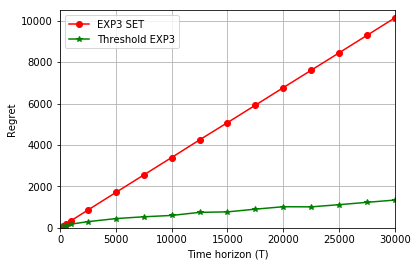
(a) For $\alpha(G)=5$

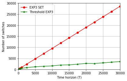
(b) For $\alpha(G)=5$

Figure 1: Performance evaluation of EXP3 SET and Threshold based EXP3 for K=25

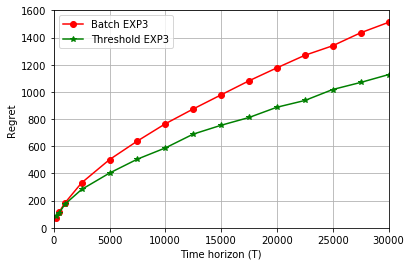
(a) For $K=5$

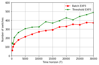
(b) For $K=5$

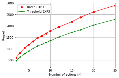
(c) For $T=20000$

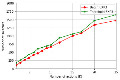
(d) For $T=20000$

Figure 2: Performance evaluation of Batch EXP3 and Threshold based EXP3 in MAB setting

6 Conclusion

This work focuses on online learning in the PI setting with SC in the presence of an adversary. The lower bound on the expected regret is presented in the PI setup in terms of independence sequence number. There is a need to design new algorithms in this setting because any algorithm that is order optimal without SC is necessarily sub-optimal in the presence of SC. Two algorithms, Threshold Based EXP3 and EXP3.SC, are proposed and their performance is evaluated in terms of expected regret. These algorithms are order optimal in $T$ in two cases: symmetric PI and MAB setup. Numerical comparisons show that the Threshold Based EXP3 outperforms EXP3 SET and Batch EXP3 in PI setting with SC.

As future work, algorithms can be designed in a partially informed setting and a fully informed setting. In the partially informed setting, the feedback graph $G_{t}$ at round $t$ is revealed following the action at round $t-1$. Thus, the feedback graphs are revealed one at a time in advance at the beginning of each round. In the fully informed setting, the entire sequence of feedback graphs $G_{1:T}$ is revealed before the game starts. Since the adversary is aware of $G_{1:T}$, these settings are important to study from the player’s end as well. Note that without SC, the algorithms in both the partially informed and fully informed settings can exploit the feedback graphs at every round in a greedy manner, and perform an action accordingly. Hence, the algorithm in partially informed setting is also optimal in a fully informed setting in the absence of SC. On the contrary, in the presence of SC, a greedy exploitation of the feedback structure is not possible at every round. Hence, in fully informed setting with SC, the player chooses an action based on $G_{1:T}$ such that the selected action balances the trade off between the regret and the SC. Thus, the partially informed and fully informed settings of PI are of particular interest in the presence of SC, and is an interesting area for further study.

Appendix A Proof of Theorem 1

Proof.

Without loss of generality, let the independent sequence set $\mathcal{I}(G_{1:T})$ formed of actions (or “arms”) from $1$ to $\beta(G_{1:T})$. Given the sequence of feedback graphs $G_{1:T}$, let $T_{i}$ be the number of times the action $i\in\mathcal{I}(G_{1:T})=[\beta(G_{1:T})]$ is selected by the player in $T$ rounds. Let $T_{\Delta}$ be the total number of times the actions are selected from the set $[K]\backslash\mathcal{I}(G_{1:T})$. Let $\mathbb{E}_{i}$ denote expectation conditioned on $X=i$, and $\mathbb{P}_{i}$ denote the probability conditioned on $X=i$. Additionally, we define $\mathbb{P}_{0}$ as the probability conditioned on event $\epsilon_{1}=0$. Therefore, under $\mathbb{P}_{0}$ , all the actions in the independent sequence set, i.e. $i\in\mathcal{I}(G_{1:T})$, incur an expected regret of $1/2$, whereas, the expected regret of actions $i\in[K]\backslash\mathcal{I}(G_{1:T})$ is $1/2+\epsilon_{2}$. Let $\mathbb{E}_{0}$ be the corresponding conditional expectation. For all $i\in[K]$ and $t\leq T$, $\ell_{t}({i})$ and $\ell^{c}_{t}({i})$ denote the unclipped and clipped loss of the action $i$ respectively. Assuming the unclipped losses are observed by the player, then $\mathcal{F}$ is the sigma field generated by the unclipped losses, and $S_{t}{(i_{t})}$ is the set of actions whose losses are observed at time $t$, following the selection of $i_{t}$, according to the feedback graph $G_{t}$. The observed sequence of unclipped losses will be referred as $\ell^{o}_{1:T}$. Additionally, $\mathcal{F}^{\prime}$ is the sigma field generated by the clipped losses, for all $t\in[T]$, $\ell^{\prime}_{t}(i)$ where $i\in S_{t}{(i_{t})}$, and the observed sequence of clipped losses will be referred as $\ell^{\prime o}_{1:T}$. By definition, $\mathcal{F}^{\prime}\subseteq\mathcal{F}$.

Let $i_{1},\ldots,i_{T}$ be the sequence of actions selected by a player over the time horizon $T$. Then, the regret $R^{c}$ of the player corresponding to clipped loses is

$$R^{c}=\sum_{t=1}^{T}\ell^{c}_{t}(i_{t})+c\cdot M_{s}-\min_{i\in[K]}\sum_{t=1}^{T}\ell^{c}_{t}(i),$$ (11)

where $M_{s}$ is the number of switches in the action selection sequence $i_{1},\ldots,i_{T}$, and $c$ is the cost of each switch in action. Now, we define the regret $R$ which corresponds to the unclipped loss function in Algorithm 1 as following

$$R=\sum_{t=1}^{T}\ell_{t}(i_{t})+c\cdot M_{s}-\min_{i\in[K]}\sum_{t=1}^{T}\ell_{t}(i).$$ (12)

Using (Dekel et al.,, 2014, Lemma 4), we have

$$\mathbb{P}\bigg{(}\mbox{For all }t\in[T],\frac{1}{2}+W_{t}\in\bigg{[}\frac{1}{6},\frac{5}{6}\bigg{]}\bigg{)}\geq\frac{5}{6}.$$ (13)

Thus, for all $T>\max\{\beta(G_{1:T}),6\}$, we have $\epsilon_{1}=\epsilon_{2}<1/6$. If $B=\{\mbox{For all }t\in[T]:{1}/{2}+W_{t}\in[{1}/{6},{5}/{6}]\}$ occurs and $\epsilon_{1}=\epsilon_{2}<1/6$, then for all $i\in[K]$, $\ell^{c}_{t}(i)=\ell_{t}(i)$ which implies $R^{c}=R$ (see (11) and (12)). Now, if the event $B$ does not occur, then the losses at any time $t$ satisfy

$$\ell_{t}(i)-\ell^{c}_{t}(i)\leq(\epsilon_{1}+\epsilon_{2}).$$

Therefore, we have

$$c\cdot M_{s}\leq R^{c}\leq R\leq c\cdot M_{s}+(\epsilon_{1}+\epsilon_{2})T.$$

Now, for $T>\max\{\beta(G_{1:T}),6\}$, we have

$$\mathbb{E}[R]-\mathbb{E}[R^{c}]=(1-\mathbb{P}(B))\mathbb{E}[R-R^{c}|B\mbox{ does not occur}]\leq\frac{(\epsilon_{1}+\epsilon_{2})T}{6}.$$ (14)

Thus, (14) lower bounds the actual regret $R^{c}$ in terms of regret $R$. Now, we derive the lower bound on regret $R$ corresponding to the unclipped loses. Using the definition of $R$, we have

$$\begin{split}&\mathbb{E}[R]=\max_{i\in[K]}\mathbb{E}[\sum_{t=1}^{T}\ell_{t}(i_{t})-\sum_{t=1}^{T}\ell_{t}(i)]+\mathbb{E}[M_{s}]\\ &=\frac{1}{\beta(G_{1:T})}\sum_{i=1}^{\beta(G_{1:T})}\mathbb{E}_{i}[\sum_{t=1}^{T}\ell_{t}(i_{t})-\min_{i\in[K]}\sum_{t=1}^{T}\ell_{t}(i)]+\mathbb{E}[M_{s}]\\ &=\frac{1}{\beta(G_{1:T})}\sum_{i=1}^{\beta(G_{1:T})}\mathbb{E}_{i}\bigg{[}\sum_{j\in\mathcal{I}(G_{1:T})\backslash\{i\}}\frac{1}{2}T_{j}+\bigg{(}\frac{1}{2}-\epsilon_{1}\bigg{)}T_{i}+\bigg{(}\frac{1}{2}+\epsilon_{2}\bigg{)}T_{\Delta}-\bigg{(}\frac{1}{2}-\epsilon_{1}\bigg{)}T\Bigg{]}+\mathbb{E}[M_{s}]\\ &=\frac{1}{\beta(G_{1:T})}\sum_{i=1}^{\beta(G_{1:T})}\mathbb{E}_{i}\Bigg{[}\sum_{j=1}^{\beta(G_{1:T})}\frac{1}{2}T_{j}+\bigg{(}\frac{1}{2}+\epsilon_{2}\bigg{)}T_{\Delta}-\epsilon_{1}T_{i}-\bigg{(}\frac{1}{2}-\epsilon_{1}\bigg{)}T\Bigg{]}+\mathbb{E}[M_{s}]\\ &\stackrel{{\scriptstyle(a)}}{{=}}\frac{1}{\beta(G_{1:T})}\sum_{i=1}^{\beta(G_{1:T})}\mathbb{E}_{i}\Bigg{[}\epsilon_{2}T_{\Delta}+\epsilon_{1}(T-T_{i})\Bigg{]}+\mathbb{E}[M_{s}]\\ &\stackrel{{\scriptstyle(b)}}{{\geq}}\epsilon_{1}\Bigg{(}T-\frac{1}{\beta(G_{1:T})}\sum_{i=1}^{\beta(G_{1:T})}\mathbb{E}_{i}\big{[}T_{i}\big{]}+\mathbb{E}\big{[}T_{\Delta}\big{]}\Bigg{)}+\mathbb{E}[M_{s}],\end{split}$$ (15)

where $(a)$ follows from $\sum_{j=1}^{\beta(G_{1:T})}T_{j}+T_{\Delta}=T$, and $(b)$ follows from $\epsilon_{1}=\epsilon_{2}$.

Now, we upper bound the $\mathbb{E}_{i}\big{[}T_{i}\big{]}$ in (15) to obtain the lower bound on the expected regret $\mathbb{E}[R]$. Since the player is deterministic, the event $\{i_{t}=i\}$ is $\mathcal{F}^{\prime}$ measurable. Therefore, we have

$$\mathbb{P}_{i}(i_{t}=i)-\mathbb{P}_{0}(i_{t}=i)\leq d_{TV}^{\mathcal{F}^{\prime}}({P}_{0},{P}_{i})\stackrel{{\scriptstyle(a)}}{{\leq}}d_{TV}^{\mathcal{F}}({P}_{0},{P}_{i}),$$

where $d_{TV}^{\mathcal{F}}({P}_{0},{P}_{i})=\sup_{A\in\mathcal{F}}\lvert\mathbb{P}_{0}(A)-\mathbb{P}_{i}(A)\rvert$ is the total variational distance between the two probability measures, and $(a)$ follows from $\mathcal{F}^{\prime}\subseteq\mathcal{F}$. Summing the above equation over $t\in[T]$ and $i\in\mathcal{I}(G_{1:T})$ yields

$$\sum_{i=1}^{\beta(G_{1:T})}\big{(}\mathbb{E}_{i}[T_{i}]-\mathbb{E}_{0}[T_{i}]\big{)}\leq T\cdot\sum_{i=1}^{\beta(G_{1:T})}d_{TV}^{\mathcal{F}}({P}_{0},{P}_{i}).$$

Rearranging the above equation and using $\sum_{i=1}^{\beta(G_{1:T})}\mathbb{E}_{0}[T_{i}]=\mathbb{E}_{0}[\sum_{i=1}^{\beta(G_{1:T})}T_{i}]=T$, we get

$$\sum_{i=1}^{\beta(G_{1:T})}\mathbb{E}_{i}[T_{i}]\leq T\cdot\sum_{i=1}^{\beta(G_{1:T})}d_{TV}^{\mathcal{F}}({P}_{0},{P}_{i})+T.$$

Combining the above equation with (15), we get

$$\begin{split}\mathbb{E}[R]&\geq\epsilon_{1}T-\frac{\epsilon_{1}T}{\beta(G_{1:T})}\cdot\sum_{i=1}^{\beta(G_{1:T})}d_{TV}^{\mathcal{F}}({P}_{0},{P}_{i})-\frac{\epsilon_{1}T}{\beta(G_{1:T})}+\frac{\epsilon_{1}}{\beta(G_{1:T})}\sum_{i=1}^{\beta(G_{1:T})}\mathbb{E}_{i}\big{[}T_{\Delta}\big{]}+\mathbb{E}[M_{s}]\\ &\stackrel{{\scriptstyle(a)}}{{\geq}}\frac{\epsilon_{1}T}{2}-\frac{\epsilon_{1}T}{\beta(G_{1:T})}\cdot\sum_{i=1}^{\beta(G_{1:T})}d_{TV}^{\mathcal{F}}({P}_{0},{P}_{i})+{\epsilon_{1}}\mathbb{E}\big{[}T_{\Delta}\big{]}+\mathbb{E}[M_{s}],\end{split}$$ (16)

where $(a)$ uses the fact that $\beta(G_{1:T})>1$. Next, we upper bound the second term in the right hand side of (16). Using Pinsker’s inequality, we have

$$d_{TV}^{\mathcal{F}}({P}_{0},{P}_{i})\leq\sqrt{\frac{1}{2}D_{KL}(\mathbb{P}_{0}(\ell^{o}_{1:T})||\mathbb{P}_{i}(\ell^{o}_{1:T}))},$$ (17)

where $\ell^{o}_{1:T}$ are the losses observed by the player over the time horizon $T$. Using the chain rule of relative entropy to decompose $D_{KL}(\mathbb{P}_{0}(\ell^{o}_{1:T})||\mathbb{P}_{0}(\ell^{o}_{1:T}))$, we get

$$\begin{split}D_{KL}(\mathbb{P}_{0}(\ell^{o}_{1:T})||\mathbb{P}_{i}(\ell^{o}_{1:T}))&=\sum_{t=1}^{T}D_{KL}(\mathbb{P}_{0}(\ell_{t}^{o}|\ell^{o}_{1:t-1})||\mathbb{P}_{i}(\ell^{o}_{t}|\ell^{o}_{1:t-1}))\\ &=\sum_{t=1}^{T}D_{KL}(\mathbb{P}_{0}(\ell^{o}_{t}|\ell^{o}_{\rho^{*}(t)})||\mathbb{P}_{i}(\ell^{o}_{t}|\ell^{o}_{\rho^{*}(t)})),\end{split}$$ (18)

where $\rho^{*}(t)$ is the set of time instances $0\leq k\leq t$ encountered when operation $\rho(.)$ in Algorithm 1 is applied recursively to $t$. Now, we deal with each term $D_{KL}(\mathbb{P}_{0}(\ell^{o}_{t}|\ell^{o}_{\rho^{*}(t)})||\mathbb{P}_{i}(\ell^{o}_{t}|\ell^{o}_{\rho^{*}(t)}))$ in the summation individually. For $i\in\mathcal{I}(G_{1:T})$, we separate this computation into four cases: $i_{t}$ is such that loss of action $i$ is observed at both time instances $t$ and $\rho(t)$ i.e. $i\in S_{t}(i_{t})$ and $i\in S_{t}(i_{\rho(t)})$; $i_{t}$ is such that loss of action $i$ is observed at time instance $t$ but not at time instance $\rho(t)$ i.e. $i\in S_{t}(i_{t})$ and $i\notin S_{t}(i_{\rho(t)})$; $i_{t}$ is such that loss of action $i$ is not observed at time instance $t$ but is observed at time instance $\rho(t)$ i.e. $i\notin S_{t}(i_{t})$ and $i\in S_{t}(i_{\rho(t)})$; $i_{t}$ is such that loss of action $i$ is not observed at both time instances $t$ and $\rho(t)$ i.e. $i\notin S_{t}(i_{t})$ and $i\notin S_{t}(i_{\rho(t)})$.

Case 1: Since the loss of action $i$ is observed from the independent sequence set $\mathcal{I}(G_{1:T})$ at both the time instances, the loss distribution for the action $i$ is $\ell^{o}_{t}(i)|\ell^{o}_{\rho^{*}(t)}\sim\mathcal{N}(\ell_{\rho(t)}(i),\sigma^{2})$ for both $\mathbb{P}_{0}$ and $\mathbb{P}_{i}$. For all $j\in[K]\backslash\mathcal{I}(G_{1:T})$, the loss distribution is $\ell^{o}_{t}(j)|\ell^{o}_{\rho^{*}(t)}\sim\mathcal{N}(\ell_{\rho(t)}(i)+\epsilon_{1}+\epsilon_{2},\sigma^{2})$ under both $\mathbb{P}_{0}$ and $\mathbb{P}_{i}$.

Case 2: Since the loss of action $i$ is observed from the independent sequence set $\mathcal{I}(G_{1:T})$ at time instance $t$ but not at $\rho(t)$, therefore, there exists an action $k^{\prime}\in\mathcal{I}(G_{1:T})\backslash\{i\}$ from the independent sequence set which was observed at time instance $\rho(t)$. Then, the loss distribution for the action $i$ is $\ell_{t}^{o}(i)|\ell^{o}_{\rho^{*}(t)}\sim\mathcal{N}(\ell_{\rho(t)}(k^{\prime}),\sigma^{2})$ under $\mathbb{P}_{0}$, and $\ell^{o}_{t}(i)|\ell^{o}_{\rho^{*}(t)}\sim\mathcal{N}(\ell_{\rho(t)}(k^{\prime})-\epsilon_{1},\sigma^{2})$ under $\mathbb{P}_{i}$. For all $j\in[K]\backslash\mathcal{I}(G_{1:T})$, the loss distribution is $\ell^{o}_{t}(j)|\ell^{o}_{\rho^{*}(t)}\sim\mathcal{N}(\ell_{\rho(t)}(k^{\prime})+\epsilon_{2},\sigma^{2})$ under both $\mathbb{P}_{0}$ and $\mathbb{P}_{i}$.

Case 3:Since the action $i$ is observed from the independent sequence set $\mathcal{I}(G_{1:T})$ at time instance $\rho(t)$ but not at $t$, therefore, there exists an action $k^{\prime}\in\mathcal{I}(G_{1:T})\backslash\{i\}$ from the independent sequence set which was observed at time instance $t$. Then, the loss distribution for the arm $k^{\prime}$ is $\ell^{o}_{t}(k^{\prime})|\ell^{o}_{\rho^{*}(t)}\sim\mathcal{N}(\ell_{\rho(t)}(i),\sigma^{2})$ under $\mathbb{P}_{0}$, and $\ell^{o}_{t}(k^{\prime})|\ell^{o}_{\rho^{*}(t)}\sim\mathcal{N}(\ell_{\rho(t)}(i)+\epsilon_{1},\sigma^{2})$ under $\mathbb{P}_{i}$. For all $j\in[K]\backslash\mathcal{I}(G_{1:T})$, the loss distribution is $\ell^{o}_{t}(j)|\ell^{o}_{\rho^{*}(t)}\sim\mathcal{N}(\ell_{\rho(t)}(i)+\epsilon_{1}+\epsilon_{2},\sigma^{2})$ under both $\mathbb{P}_{0}$ and $\mathbb{P}_{i}$.

Case 4: Let $k^{*}$ be the arm from the independent sequence set observed at time instance $\rho(t)$. Since the arm $i$ is not observed from the independent sequence set $\mathcal{I}(G_{1:T})$ at the time instances $t$ and $\rho(t)$, therefore the loss distribution for all arms $k^{\prime}\in\mathcal{I}(G_{1:T})\backslash\{i\}$ is $\ell^{o}_{t}(k^{\prime})|\ell^{o}_{\rho^{*}(t)}\sim\mathcal{N}(\ell_{\rho(t)}(k^{*}),\sigma^{2})$ for both $\mathbb{P}_{0}$ and $\mathbb{P}_{i}$. For all $j\in[K]\backslash\mathcal{I}(G_{1:T})$, the loss distribution is $\ell^{o}_{t}(j)|\ell^{o}_{\rho^{*}(t)}\sim\mathcal{N}(\ell_{\rho(t)}(k^{*})+\epsilon_{2},\sigma^{2})$ under both $\mathbb{P}_{0}$ and $\mathbb{P}_{i}$.

Therefore, we have

$$\begin{split}D_{KL}(\mathbb{P}_{0}(\ell^{o}_{t}|\ell^{o}_{\rho^{*}(t)})||\mathbb{P}_{i}(\ell^{o}_{t}|\ell^{o}_{\rho^{*}(t)}))&=\mathbb{P}_{0}(i\in S_{t}{(i_{t})},i\notin S_{\rho(t)}({i_{\rho(t)}}))\cdot D_{KL}(\mathcal{N}(0,\sigma^{2})||\mathcal{N}(-\epsilon_{1},\sigma^{2}))\\ &+\mathbb{P}_{0}(i\notin S_{t}({i_{t}}),i\in S_{\rho(t)}({i_{\rho(t)}}))\cdot D_{KL}(\mathcal{N}(0,\sigma^{2})||\mathcal{N}(\epsilon_{1},\sigma^{2}))\\ &=\frac{\epsilon_{1}^{2}}{2\sigma^{2}}\mathbb{P}_{0}(B_{t}),\end{split}$$ (19)

where $B_{t}=\{i\in S_{t}({i_{t}}),i\notin S_{\rho(t)}({i_{\rho(t)}})\cup i\notin S_{t}{(i_{t})},i\in S_{\rho(t)}{(i_{\rho(t)})}\}$. The event $B_{t}$ implies that at least one of the following events are true:
$(i)$ The player has switched between the feedback systems $S_{t}{(k_{1})}$ and $S_{\rho(t)}{(k_{2})}$ such that $i\in S_{t}{(k_{1})}$ but $i\notin S_{\rho(t)}{(k_{2})}$ or vice-versa.
$(ii)$ The player did not change the selection of action, however, the feedback system has changed between $\rho(t)$ and $t$ such that $i$ has become observable or vice versa. This can occur only if the fixed action belongs to $[K]\setminus\mathcal{I}(G_{1:T})$.
Let $N_{i}$ be the number of times a player switches from the feedback system which includes $i$ to the feedback system which does not include $i$ and vice-versa. Then, using (18) and (19), we have

$$D_{KL}(\mathbb{P}_{0}(\ell^{o}_{1:T})||\mathbb{P}_{i}(\ell^{o}_{1:T}))\leq\frac{\epsilon_{1}^{2}\omega(\rho)}{2\sigma^{2}}\mathbb{E}_{0}[N_{i}+T_{\Delta}],$$ (20)

where $\omega(\rho)$ is the width of process $\rho(.)$ (see Definition 2 in Dekel et al., (2014)) and is bounded above by $2\log_{2}(T)$. Combining (17) and (20), we have

$$\sup_{A\in\mathcal{F}}(\mathbb{P}_{0}(A)-\mathbb{P}_{i}(A))\leq\frac{\epsilon_{1}}{\sigma}\sqrt{\log_{2}(T)\mathbb{E}_{0}[N_{i}+T_{\Delta}]}.$$ (21)

If $M_{s}\geq\epsilon_{1}T$, then $\mathbb{E}[R^{\prime}]>\epsilon_{1}T$. Thus, the claimed lower bound follows. Now, let us assume $M_{s}\leq\epsilon_{1}T$. For all $i\in\mathcal{I}(G_{1:T})$, we have

$$\begin{split}\mathbb{E}_{0}[M_{s}]-\mathbb{E}_{i}[M_{s}]&=\sum_{m=1}^{\lfloor\epsilon_{1}T\rfloor}\mathbb{P}_{0}(M_{s}\geq m)-\mathbb{P}_{i}(M_{s}\geq m))\\ &\leq\epsilon_{1}T\cdot d_{TV}^{\mathcal{F}}(\mathbb{P}_{0},\mathbb{P}_{i}).\end{split}$$ (22)

Using the above equation, we have

$$\begin{split}\mathbb{E}_{0}[M_{s}]-\mathbb{E}[M_{s}]&=\frac{1}{\beta(G_{1:T})}\sum_{i=1}^{\beta(G_{1:T})}(\mathbb{E}_{0}[M_{s}]-\mathbb{E}_{i}[M_{s}])\\ &\leq\frac{\epsilon_{1}T}{\beta(G_{1:T})}\sum_{i=1}^{\beta(G_{1:T})}d_{TV}^{\mathcal{F}}(\mathbb{P}_{0},\mathbb{P}_{i}).\end{split}$$ (23)

Now, combining (14), (16), (21)and (23), we obtain

$$\begin{split}\mathbb{E}[R^{\prime}]&\geq\frac{\epsilon_{1}T}{6}-\frac{\epsilon_{1}T}{\beta(G_{1:T})}\sum_{i=1}^{\beta(G_{1:T})}\frac{\epsilon_{1}}{\sigma}\sqrt{\log_{2}(T)\mathbb{E}_{0}[N_{i}+T_{\Delta}]}+{\epsilon_{1}}\mathbb{E}\big{[}T_{\Delta}\big{]}+c\cdot\mathbb{E}_{0}[M_{s}]\\ &\stackrel{{\scriptstyle(a)}}{{\geq}}\frac{\epsilon_{1}T}{6}-\frac{\epsilon_{1}^{2}T}{\sigma\sqrt{\beta(G_{1:T})}}\sqrt{2\log_{2}(T)\mathbb{E}_{0}[M_{s}+T_{\Delta}]}+{\epsilon_{1}}\mathbb{E}\big{[}T_{\Delta}\big{]}+c\cdot\mathbb{E}_{0}[M_{s}]\\ &\stackrel{{\scriptstyle(b)}}{{\geq}}\frac{\epsilon_{1}T}{6}-\frac{\epsilon_{1}^{4}T^{2}\log_{2}(T)}{c\cdot\sigma^{2}\beta(G_{1:T})}+{\epsilon_{1}}\mathbb{E}\big{[}T_{\Delta}\big{]}+c\cdot\bigg{(}\frac{\epsilon_{1}^{4}T^{2}\log_{2}(T)}{2c^{2}\cdot\sigma^{2}\beta(G_{1:T})}-\mathbb{E}_{0}\big{[}T_{\Delta}\big{]}\bigg{)},\\ &\stackrel{{\scriptstyle}}{{\geq}}\frac{c^{1/3}\beta(G_{1:T})^{1/3}T^{2/3}}{54\log_{2}(T)}-\frac{c^{1/3}\beta(G_{1:T})^{1/3}T^{2/3}}{162\log_{2}(T)}+(\epsilon_{1}-c)\mathbb{E}_{0}\big{[}T_{\Delta}\big{]}\\ &\stackrel{{\scriptstyle(c)}}{{\geq}}\frac{c^{1/3}\beta(G_{1:T})^{1/3}T^{2/3}}{81\log_{2}(T)},\end{split}$$ (24)

where $(a)$ follows from the concavity of $\sqrt{x}$ and $\sum_{i}^{\beta(G_{1:T})}N_{i}\leq 2M_{s}$, $(b)$ follows from the fact that the right hand side is minimized for $\sqrt{\mathbb{E}_{0}[M_{s}+T_{\Delta}]}=\epsilon^{2}T\sqrt{\log_{2}(T)}/2c\sigma\sqrt{\beta(G_{1:T})}$, and $(c)$ follows from the assumption $T\geq 27c\log_{2}^{3/2}(T)/\beta(G_{1:T})^{2}$, which implies $\epsilon_{1}\geq c$. The claim of the theorem now follows. ∎

Appendix B Proof of Lemma 2

We have that $\beta(G_{1:T})$ actions are non adjacent in the entire sequence of feedback graphs $G_{1:T}$. Let $1,2,\dots\beta(G_{1:T})$ belong to the $\mathcal{I}(G_{1:T})$. Then, the adversary selects an action uniformly at random from the set $\mathcal{I}(G_{1:T})$ say $j$, and assigns the loss sequence to action $j$ using independent Bernoulli random variable with parameter $0.5-\epsilon$, where $\epsilon=\sqrt{\beta(G_{1:T})/T)}$. For all $i\in\mathcal{I}(G_{1:T})/\{j\}$, losses are assigned using independent Bernoulli random variable with parameter $0.5$. For all $i\notin\mathcal{I}(G_{1:T})$, the losses are assigned using independent Bernoulli random variable with parameter $1$. The proof of the lemma follows along the same lines as in Theorem 5 in (Alon et al., (2017)).

Appendix C Proof of Theorem 3

Proof of this theorem uses the results from Theorem 1. Since the loss sequence is assigned independently to each sub-sequence $U_{m}$ where $m\in[M]$. Using Theorem 1, there exists a constant $b_{m}$ such that

$$\begin{split}&\mathbf{E}\Bigg{[}\sum_{t=1}^{T}(\ell_{t}(i_{t})\mathbf{1}(G_{t}\in U_{m})+cW_{m}\Bigg{]}-\min_{i\in U_{m}}\sum_{t=1}^{T}(\ell_{t}(i)\mathbf{1}(G_{t}\in U_{m})\\ &\geq b_{m}c^{1/3}\beta(U_{m})^{1/3}N(U_{m})^{2/3}/\log(T),\end{split}$$ (25)

where $W_{m}$ is number of switches performed within the sequence $U_{m}$. Since

$$\sum_{m\in[M]}W_{m}\leq\sum_{t=1}^{T}\mathbf{1}(i_{t}\neq i_{t-1}),$$

there exist a constant $b$ such that the expected regret of any algorithm $\mathcal{A}$ is at least

$$b\,c^{1/3}\sum_{m\in[M]}\beta(U_{m})^{1/3}N(U_{m})^{2/3}/\log T.$$

Appendix D Proof of Lemma 4

Proof.

The proof follows from contradiction and is along the same lines as the proof of Theorem 4 in Dekel et al., (2014). Let $\mathcal{A}$ performs at most $\tilde{O}((\beta(G_{1:T})^{1/2}T)^{\alpha})$ switches for any sequence of loss function over $T$ rounds with $\beta+\alpha/2<1$. Then, there exists a real number $\gamma$ such that $\beta<\gamma<1-\alpha/2$. Then, assign $c=(\beta(G_{1:T})^{1/2}T)^{3\gamma-2}$. Thus, the expected regret, including the switching cost, of the algorithm is

$$\tilde{O}((\beta(G_{1:T})^{1/2}T)^{\beta}+(\beta(G_{1:T})^{1/2}T)^{3\gamma-2}(\beta(G_{1:T})T)^{\alpha})=\tilde{o}(\beta(G_{1:T})^{1/2}T)^{\gamma},$$

over a sequence of losses assigned by the adversary because $\beta<\gamma$ and $\alpha<2-2\gamma$. However, according to Theorem 1, the expected regret is at least $\tilde{\Omega}(\beta(G_{1:T})^{1/3}(\beta(G_{1:T})^{1/2}T)^{(3\gamma-2)/3}T^{2/3})=\tilde{\Omega}((\beta(G_{1:T})T)^{\gamma})$. Hence, by contradiction, the proof of the lemma follows.

∎

Appendix E Proof of Theorem 5

Proof.

Let $t_{1},t_{2}\ldots,t_{\sigma(T)}$ be the sequence of time instances at which the event $E^{t}$ occurs during the duration $T$ of the game. We define $\{r_{j}=t_{j+1}-t_{j}\}_{1\leq j\leq T}$ as the sequence of inter-event times between the events $E^{t}$. Let $\mbox{mas}(G_{(1)}),\ldots,\mbox{mas}(G_{(T)})$ denote the sequence in the decreasing order of size of maximal acyclic graphs, i.e. $\mbox{mas}(G_{(1)})$ (or $\mbox{mas}(G_{(T)})$) is the maximum (or minimum) size of maximal acyclic graph observed in sequence $G_{1:T}=\{G_{1},\ldots G_{T}\}$. Using the definition of $E^{t}$, note that $r_{j}$ is a random variable bounded by $T^{1/3}c^{2/3}/\mbox{mas}(G_{(T)})^{1/3}$. For all $1\leq j\leq\sigma(T)$, the ratio of total weights of actions at round $t_{j}$ and $t_{j+1}$ is

$$\begin{split}\frac{W_{t_{j+1}}}{W_{t_{j}}}&=\sum_{i\in[K]}\frac{w_{i,t_{j+1}}}{W_{t_{j}}}\\ &=\sum_{i\in[K]}\frac{w_{i,t_{j}}\exp(-\eta\ell^{\prime}_{t_{j}+r_{j}-1}(i))}{W_{t_{j}}}\\ &=\sum_{i\in[K]}p_{i,t_{j}}\exp(-\eta\ell^{\prime}_{t_{j}+r_{j}-1}(i))\\ &\stackrel{{\scriptstyle(a)}}{{\leq}}\sum_{i\in[K]}p_{i,t_{j}}\bigg{(}1-\eta\ell^{\prime}_{t_{j}+r_{j}-1}(i)+\frac{1}{2}\eta^{2}\ell^{\prime 2}_{t_{j}+r_{j}-1}(i)\bigg{)}\\ &=1-\eta\sum_{i\in[K]}p_{i,t_{j}}\cdot\ell^{\prime}_{t_{j}+r_{j}-1}(i)+\frac{\eta^{2}}{2}\sum_{i\in[K]}p_{i,t_{j}}\cdot\ell^{\prime 2}_{t_{j}+r_{j}-1}(i),\end{split}$$ (26)

where $(a)$ follows from the fact that, for all $x\geq 0$, $e^{-x}\leq 1-x-x^{2}/2$. Now, taking logs on both sides of (26), summing over $t_{1},t_{2},\ldots t_{\sigma(T)}$, and using $\log(1+x)\leq x$ for all $x>-1$, we get

$$\log\frac{W_{t_{\sigma(T)+1}}}{W_{1}}\leq-\eta\sum_{j=1}^{\sigma(T)}\sum_{i\in[K]}p_{i,t_{j}}\cdot\ell^{\prime}_{t_{j}+r_{j}-1}(i)+\frac{\eta^{2}}{2}\sum_{j=1}^{\sigma(T)}\sum_{i\in[K]}p_{i,t_{j}}\cdot\ell^{\prime 2}_{t_{j}+r_{j}-1}(i).$$ (27)

For all actions $k^{\prime}\in[K]$, we also have

$$\log\frac{W_{t_{\sigma(T)+1}}}{W_{1}}\geq\log\frac{w_{k^{\prime},t_{\sigma(T)+1}}}{W_{1}}\geq-\eta\sum_{j=1}^{\sigma(T)}\ell^{\prime}_{t_{j}+r_{j}-1}(k^{\prime})-\log(K).$$ (28)

Combining (27) and (28), for all $k^{\prime}\in[K]$, we obtain

$$\sum_{j=1}^{\sigma(T)}\sum_{i\in[K]}p_{i,t_{j}}\cdot\ell^{\prime}_{t_{j}+r_{j}-1}(i)-\sum_{j=1}^{\sigma(T)}\ell^{\prime}_{t_{j}+r_{j}-1}(k^{\prime})\leq\frac{\log(K)}{\eta}+\frac{\eta}{2}\sum_{j=1}^{\sigma(T)}\sum_{i\in[K]}p_{i,t_{j}}\cdot\ell^{\prime 2}_{t_{j}+r_{j}-1}(i).$$ (29)

Now, for all $i\in[K]$, the conditional expectation of $\ell^{\prime}_{t_{j}+r_{j}-1}(i)$ is

$$\begin{split}\mathbb{E}\bigg{[}\ell^{\prime}_{t_{j}+r_{j}-1}(i)\Big{|}p_{t_{j}},r_{j}\bigg{]}&=\sum_{t=t_{j}}^{t_{j}+r_{j}-1}\sum_{k^{\prime}:i\in S_{t}(k^{\prime})}p_{k^{\prime},t_{j}}\cdot\frac{\ell_{t}(i)}{q_{i,t}},\\ &=\sum_{t=t_{j}}^{t_{j}+r_{j}-1}\frac{\ell_{t}(i)}{q_{i,t}}\cdot\sum_{k^{\prime}:i\in S_{t}(k^{\prime})}p_{k^{\prime},t_{j}},\\ &=\sum_{t=t_{j}}^{t_{j}+r_{j}-1}\ell_{t}(i).\end{split}$$ (30)

Therefore, we have that for all $i\in[K]$, the conditional expectation

$$\mathbb{E}\bigg{[}\sum_{j=1}^{\sigma(T)}\ell^{\prime}_{t_{j}+r_{j}-1}(i)\Big{|}\{p_{t_{j}},r_{j}\}_{1\leq j\leq\sigma(T)}]\bigg{]}=\sum_{j=1}^{\sigma(T)}\sum_{t=t_{j}}^{t_{j}+r_{j}-1}\ell_{t}(i)=\sum_{t=1}^{T}\ell_{t}(i).$$ (31)

Now, the expectation of second term in right hand side of (29) is

$$\begin{split}\mathbb{E}\left[\sum_{j=1}^{\sigma(T)}\sum_{i\in[K]}p_{i,t_{j}}\cdot\ell^{\prime 2}_{t_{j}+r_{j}-1}(i)\right]&=\mathbb{E}\Bigg{[}\sum_{j=1}^{\sigma(T)}\mathbb{E}\bigg{[}\sum_{i\in[K]}p_{i,t_{j}}\ell^{\prime 2}_{t_{j}+r_{j}-1}(i)|\{p_{t_{j}},r_{j}\}_{1\leq j\leq\sigma(T)}\bigg{]}\Bigg{]}\\ &\stackrel{{\scriptstyle(a)}}{{\leq}}\mathbb{E}\Bigg{[}\sum_{j=1}^{\sigma(T)}\mbox{mas}(G_{t_{j}:t_{j}+r_{j}-1}){r^{2}_{j}}\Bigg{]},\\ \end{split}$$ (32)

where $\mbox{mas}(G_{t_{j}:t_{j}+r_{j}-1})=\max_{n\in[t_{j},t_{j}+r_{j}-1]}\mbox{mas}(G_{n})$, and $(a)$ follows from the fact that, for all $i\in[K]$ and $t\leq T$, $\ell_{t}(i)\leq 1$, and $\sum_{i\in[K]}p_{i,t}/q_{i,t}\leq\mbox{mas}(G_{t})$(Alon et al.,, 2017, Lemma 10).

Now, we bound $\sum_{j=1}^{\sigma(T)}\mbox{mas}(G_{t_{j}:t_{j}+r_{j}-1}){r^{2}_{j}}$. We write the following optimization problem:

$$\max_{\{r_{j}\}_{1\leq j\leq T}}\sum_{j=1}^{T}\mbox{mas}(G_{t_{j}:t_{j}+r_{j}-1}){r^{2}_{j}},\mbox{ subject to}$$ (33)

$$\sum_{j=1}^{T}r_{j}=T,$$

$$0\leq r_{j}\leq\frac{T^{1/3}c^{2/3}}{\mbox{mas}^{1/3}(G_{(T)})}.$$

Since the objective function is submodular and the constraints are linear, the ratio of the solution of the greedy algorithm and the optimal solution is at most $(1-1/e)$ (Nemhauser and Wolsey, (1978)). Therefore, the optimal solution $o^{*}$ of the above optimization problem is

$$o^{*}\leq\sum_{t=1}^{t^{*}}\frac{T^{2/3}\mbox{mas}(G_{(t)})c^{4/3}}{(1-1/e)\mbox{mas}^{2/3}(G_{(T)})},$$ (34)

where $t^{*}={\lceil T^{2/3}c^{-2/3}\mbox{mas}^{1/3}(G_{(T)})\rceil}$. Using (29), (30), (31), (32) and (34), we have

$$\mathbb{E}\Bigg{[}\sum_{j=1}^{\sigma(T)}\sum_{i\in[K]}p_{i,k_{j}}\sum_{t=k_{j}}^{k_{j}+r_{j}-1}\ell_{t}(i)-\sum_{j=1}^{T}\ell_{t}({k^{\prime}})\Bigg{]}\leq\frac{\log(K)}{\eta}+\frac{\eta}{2}\sum_{t=1}^{t^{*}}\frac{T^{2/3}c^{4/3}\mbox{mas}(G_{(t)})}{(1-1/e)\mbox{mas}^{2/3}(G_{(T)})}.$$ (35)

Additionally, the player switches its action only if $E^{t}$ is true. Thus, using (35) and $c(i,j)=c$, for all $i,j\in[K]$, we have

$$R^{\mathcal{A}}(l_{1:T},\mathcal{C})\leq\frac{\log(K)}{\eta}+\frac{\eta}{2}\sum_{t=1}^{t^{*}}\frac{T^{2/3}c^{4/3}\mbox{mas}(G_{(t)})}{(1-1/e)\mbox{mas}^{2/3}(G_{(T)})}+c\cdot\mathbb{E}[\sum_{t=2}^{T}\textbf{1}(i_{t}\neq i_{t-1})].$$ (36)

Now, we bound $\mathbb{E}[\sum_{t=2}^{T}\textbf{1}(i_{t}\neq i_{t-1})]$. $E^{t}_{1}$ occurs with probability 1, and does not contribute to any SC. $E^{t}_{2}$ can lead to at most $\lceil T^{2/3}c^{-2/3}\mbox{mas}^{1/3}(G_{(T)})\rceil$ switches. Now, let $E^{t}_{3}$ causes $N_{T}$ switches. Then, we have

$$\begin{split}\mathbb{E}[N_{T}]&=\mathbb{E}\left[\sum_{j=1}^{\sigma(T)}\textbf{1}(i_{t_{j+1}}\neq i_{t_{j}},E^{t_{j}}_{3}\mbox{ is true})\right]\\ &=\mathbb{E}\Bigg{[}\sum_{j=1}^{\sigma(T)}\mathbb{E}\bigg{[}\textbf{1}(i_{t_{j+1}}\neq i_{t_{j}},E^{t_{j}}_{3}\mbox{ is true})\bigg{|}\{p_{t_{j}},r_{j}\}_{1\leq j\leq\sigma(T)}\bigg{]}\Bigg{]}\\ &\leq\mathbb{E}\Bigg{[}\sum_{j=1}^{\sigma(T)}\mathbb{E}\bigg{[}\sum_{i\in[K],k^{\prime}\in[K]\backslash\{i\}}\mathbb{P}(i_{t_{j}}=i\big{|}E^{t_{j}}_{3}\mbox{ is true})\mathbb{P}(i_{t_{j+1}}=k^{\prime}\big{|}i_{t_{j}}=i)\bigg{|}\{p_{t_{j}},r_{j}\}_{1\leq j\leq\sigma(T)}\bigg{]}\Bigg{]}\\ &=\mathbb{E}\bigg{[}\sum_{j=1}^{\sigma(T)}\sum_{i\in[K],k^{\prime}\in[K]\backslash\{i\}}p_{i,t_{j}}p_{k^{\prime},t_{j+1}}\bigg{]}\\ &\stackrel{{\scriptstyle(a)}}{{\leq}}\sum_{t=1}^{T}c^{-2/3}\mbox{mas}^{1/3}(G_{(T)})t^{-1/3}=c^{-2/3}\mbox{mas}^{1/3}(G_{(T)})T^{2/3},\end{split}$$ (37)

where $(a)$ follows from Lemma 7 in this section. Thus, the number of switches are $2c^{-2/3}\mbox{mas}^{1/3}(G_{(T)})T^{2/3}$, and the SC is $2c^{1/3}\mbox{mas}^{1/3}(G_{(T)})T^{2/3}$.

Part $(iii)$ of the theorem follows by combining the results from $(i)$ and $(ii)$. Part $(iv)$ follows from the fact that if $G_{t}$ is undirected, $\mbox{mas}(G_{t})=\alpha(G_{t})$. ∎

Lemma 7.

Given $i\in[K]$ is chosen at time instance $t_{j}$, for all $k^{\prime}\in[K]\backslash\{i\}$, we have

$$p_{i,t_{j}}\cdot p_{k^{\prime},t_{j+1}}\leq(t_{j+1})^{-1/3}.$$

Proof.

Given $i$ is chosen at time instance $t_{j}$, for all $k^{\prime}\in[K]\backslash\{i\}$, we have

$$\begin{split}\frac{p_{k^{\prime},t_{j+1}}}{p_{i,t_{j+1}}}&=\frac{p_{k^{\prime},1}\exp(-\eta\hat{\ell}_{t_{j+1}}(k^{\prime}))}{p_{i,t_{j}}\exp(-\eta{\ell}^{\prime}_{t_{j}+r_{j}-1}(i))}\\ &\stackrel{{\scriptstyle(a)}}{{=}}\frac{p_{k^{\prime},1}\exp(-\eta(\hat{\ell}_{t_{j}}(k^{\prime})+{\ell}^{\prime}_{t_{j}+r_{j}-1}(k^{\prime})))}{p_{i,t_{j}}\exp(-\eta{\ell}^{\prime}_{t_{j}+r_{j}-1}(i))}\\ &\stackrel{{\scriptstyle(b)}}{{\leq}}\frac{\exp\big{(}-\eta(\hat{\ell}_{t_{j}}(k^{\prime})+{\ell}^{\prime}_{t_{j}+r_{j}-1}(k^{\prime})-{\ell}^{\prime}_{t_{j}+r_{j}-1}(i))\big{)}}{p_{i,t_{j}}}\\ &\stackrel{{\scriptstyle(c)}}{{\leq}}\frac{\exp\big{(}-\eta(\epsilon_{t_{j+1}}/\eta)\big{)}}{Kp_{i,t_{j}}}\\ &=\frac{\exp\big{(}-\epsilon_{t_{j+1}}\big{)}}{p_{i,t_{j}}},\end{split}$$ (38)

where $(a)$ follows from the fact that $\hat{\ell}_{t_{j+1}}(k^{\prime})=\hat{\ell}_{t_{j}}(k^{\prime})+{\ell}^{\prime}_{t_{j}+r_{j}-1}(k^{\prime})$; $(b)$ follows from $p_{k^{\prime},1}=1/K$; $(c)$ follows from the fact that for all $k\in[K]\backslash\{i\}$, $\hat{\ell}_{k,t-1}-{\ell}^{\prime}_{i,t-1}>\epsilon_{t}/\eta$ as the increment in ${\ell}^{\prime}_{i,t-1}$ is bounded by $1/q_{i,t-1}$. Now, replacing $\epsilon_{t}\geq\log(tc^{2}/\mbox{mas}(G_{(T)}))/3$ in (38), we have

$$p_{i,t_{j}}\cdot p_{k^{\prime},t_{j+1}}\leq c^{-2/3}\mbox{mas}^{1/3}(G_{(T)})t_{j+1}^{-1/3}.$$ (39)

∎

Appendix F Proof of Theorem 6

Proof.

We borrow the notations from the proof of Theorem 5. Using the fact that $\eta_{t}$ is decreasing in $t$ and (29), we have

$$\sum_{j=1}^{\sigma(T)}\sum_{i\in[K]}p_{i,t_{j}}\cdot\ell^{\prime}_{t_{j}+r_{j}-1}(i)-\min_{k^{\prime}\in[K]}\sum_{j=1}^{\sigma(T)}\ell^{\prime}_{t_{j}+r_{j}-1}(k^{\prime})\leq\frac{\log(K)}{\eta_{T}}+\sum_{j=1}^{\sigma(T)}\frac{\eta_{t_{j}}}{2}\sum_{i\in[K]}p_{i,t_{j}}\cdot\ell^{\prime 2}_{t_{j}+r_{j}-1}(i).$$ (40)

Now, taking expectation on both the sides and using the fact that expectation of the $\min(.)$ is smaller than the $\min(.)$ of the expectation, we have

$$\begin{split}&\mathbf{E}\Bigg{[}\sum_{j=1}^{\sigma(T)}\sum_{i\in[K]}p_{i,t_{j}}\cdot\ell^{\prime}_{t_{j}+r_{j}-1}(i)\Bigg{]}-\min_{k^{\prime}\in[K]}\mathbf{E}\Bigg{[}\sum_{j=1}^{\sigma(T)}\ell^{\prime}_{t_{j}+r_{j}-1}(k^{\prime})\Bigg{]}\\ &\leq\frac{\log(K)}{\eta_{T}}+\mathbf{E}\Bigg{[}\sum_{j=1}^{\sigma(T)}\frac{\eta_{t_{j}}}{2}\epsilon_{t_{j}}\mathbf{E}\Bigg{[}\sum_{i\in[K]}p_{i,t_{j}}\cdot\ell^{\prime 2}_{t_{j}+r_{j}-1}(i)|p_{t_{j}},r_{j},\mathbf{1}(i_{t}\mbox{ is selected using }p_{t})\Bigg{]}\Bigg{]},\\ &\stackrel{{\scriptstyle(a)}}{{\leq}}\frac{\log(K)}{\eta_{T}}+\mathbf{E}\Bigg{[}\sum_{j=1}^{\sigma(T)}\frac{\eta_{t_{j}}}{2}\epsilon_{t_{j}}\mathbf{E}[\mbox{mas}(G_{t_{j}:t_{j}+r_{j}-1}){r^{2}_{j}}|\mathbf{1}(i_{t}\mbox{ is selected using }p_{t})]\Bigg{]},\\ &\stackrel{{\scriptstyle(b)}}{{\leq}}\frac{\log(K)}{\eta_{T}}+\mathbf{E}\Bigg{[}\sum_{j=1}^{\sigma(T)}\frac{\eta_{t_{j}}}{2}\epsilon_{t_{j}}\frac{2\cdot\mbox{mas}(G_{t_{j}:t_{j}+r_{j}-1})}{\epsilon_{t_{j}}^{2}}\Bigg{]},\\ &\stackrel{{\scriptstyle}}{{=}}\frac{\log(K)}{\eta_{T}}+\mathbf{E}\Bigg{[}\sum_{j=1}^{\sigma(T)}\frac{\eta_{t_{j}}}{2}\frac{2\cdot\mbox{mas}(G_{t_{j}:t_{j}+r_{j}-1})}{\epsilon_{t_{j}}}\Bigg{]},\\ &\stackrel{{\scriptstyle(c)}}{{\leq}}\frac{\log(K)}{\eta_{T}}+\mathbf{E}\Bigg{[}\sum_{j=1}^{\sigma(T)}\frac{2\log(K)}{\mbox{mas}^{2/3}(G_{(T)})}{\mbox{mas}(G_{(j)})}\Bigg{]},\\ &\stackrel{{\scriptstyle(d)}}{{\leq}}\frac{\log(K)}{\eta_{T}}+\sum_{j=1}^{\mathbf{E}[\sigma(T)]}\frac{2\log(K)}{\mbox{mas}^{2/3}(G_{(T)})}{\mbox{mas}(G_{(j)})}\end{split}$$ (41)

where $(a)$ follows from (32), $(b)$ follows from the fact that since the probability of selecting a new action is at most $\epsilon_{t_{j}}$, the mean and the variance of the geometric random variable $r_{j}$ is bounded by $1/\epsilon_{t_{j}}^{2}$ and $(1-\epsilon_{t_{j}})/\epsilon_{t_{j}}^{2}$ respectively, $(c)$ follows from the value of $\eta_{t}$ and $\epsilon_{t}$, and $(d)$ follows from the fact that $\mbox{mas}(G_{(j)})/\mbox{mas}(G_{(T)})$ is a monotonic non increasing sequence in $j$, therefore the summation is a concave function and the inequality follows from the Jensen’s inequality.

Now, we bound the $\mathbf{E}[\sigma(T)]$ in (41). This also gives a bound on the number of switches performed by the algorithm. We have

$$\begin{split}\mathbf{E}[\sigma(T)]&=\sum_{t=1}^{T}\mathbf{E}[\mathbf{1}(i_{t}\neq i_{t-1})],\\ &\leq\sum_{t=1}^{T}\epsilon_{t},\\ &\leq 0.5\mbox{mas}^{1/3}(G_{(T)})T^{2/3}c^{1/3}\end{split}$$ (42)

∎

References

• Alon etΒ al., (2015) Alon, N., Cesa-Bianchi, N., Dekel, O., and Koren, T. (2015). Online learning with feedback graphs: Beyond bandits. In JMLR WORKSHOP AND CONFERENCE PROCEEDINGS, volumeΒ 40. Microtome Publishing.
• Alon etΒ al., (2017) Alon, N., Cesa-Bianchi, N., Gentile, C., Mannor, S., Mansour, Y., and Shamir, O. (2017). Nonstochastic multi-armed bandits with graph-structured feedback. SIAM Journal on Computing, 46(6):1785–1826.
• Alon etΒ al., (2013) Alon, N., Cesa-Bianchi, N., Gentile, C., and Mansour, Y. (2013). From bandits to experts: A tale of domination and independence. In Advances in Neural Information Processing Systems, pages 1610–1618.
• Arora etΒ al., (2012) Arora, R., Dekel, O., and Tewari, A. (2012). Online bandit learning against an adaptive adversary: from regret to policy regret. arXiv preprint arXiv:1206.6400.
• Auer etΒ al., (2002) Auer, P., Cesa-Bianchi, N., Freund, Y., and Schapire, R.Β E. (2002). The nonstochastic multiarmed bandit problem. SIAM journal on computing, 32(1):48–77.
• Auer etΒ al., (2007) Auer, P., Ortner, R., and SzepesvΓ‘ri, C. (2007). Improved rates for the stochastic continuum-armed bandit problem. In International Conference on Computational Learning Theory, pages 454–468. Springer.
• Bubeck etΒ al., (2011) Bubeck, S., Munos, R., Stoltz, G., and SzepesvΓ‘ri, C. (2011). X-armed bandits. Journal of Machine Learning Research, 12(May):1655–1695.
• Caron etΒ al., (2012) Caron, S., Kveton, B., Lelarge, M., and Bhagat, S. (2012). Leveraging side observations in stochastic bandits. arXiv preprint arXiv:1210.4839.
• Cesa-Bianchi and Lugosi, (2006) Cesa-Bianchi, N. and Lugosi, G. (2006). Prediction, learning, and games. Cambridge university press.
• Coja-Oghlan and Efthymiou, (2015) Coja-Oghlan, A. and Efthymiou, C. (2015). On independent sets in random graphs. Random Structures & Algorithms, 47(3):436–486.
• Dekel etΒ al., (2014) Dekel, O., Ding, J., Koren, T., and Peres, Y. (2014). Bandits with switching costs: T 2/3 regret. In Proceedings of the forty-sixth annual ACM symposium on Theory of computing, pages 459–467. ACM.
• Feldman etΒ al., (2016) Feldman, M., Koren, T., Livni, R., Mansour, Y., and Zohar, A. (2016). Online pricing with strategic and patient buyers. In Advances in Neural Information Processing Systems, pages 3864–3872.
• Gentile and Orabona, (2014) Gentile, C. and Orabona, F. (2014). On multilabel classification and ranking with bandit feedback. Journal of Machine Learning Research, 15(1):2451–2487.
• Geulen etΒ al., (2010) Geulen, S., VΓΆcking, B., and Winkler, M. (2010). Regret minimization for online buffering problems using the weighted majority algorithm. In COLT, pages 132–143.
• Gyorgy and Neu, (2014) Gyorgy, A. and Neu, G. (2014). Near-optimal rates for limited-delay universal lossy source coding. IEEE Transactions on Information Theory, 60(5):2823–2834.
• Katariya etΒ al., (2016) Katariya, S., Kveton, B., Szepesvari, C., and Wen, Z. (2016). Dcm bandits: Learning to rank with multiple clicks. In International Conference on Machine Learning, pages 1215–1224.
• Kleinberg, (2005) Kleinberg, R.Β D. (2005). Nearly tight bounds for the continuum-armed bandit problem. In Advances in Neural Information Processing Systems, pages 697–704.
• KocΓ‘k etΒ al., (2016) KocΓ‘k, T., Neu, G., and Valko, M. (2016). Online learning with erdΕ‘s-rΓ©nyi side-observation graphs. In Uncertainty in Artificial Intelligence.
• (19) Koren, T., Livni, R., and Mansour, Y. (2017a). Bandits with movement costs and adaptive pricing. arXiv preprint arXiv:1702.07444.
• (20) Koren, T., Livni, R., and Mansour, Y. (2017b). Multi-armed bandits with metric movement costs. In Advances in Neural Information Processing Systems, pages 4122–4131.
• Langford and Zhang, (2008) Langford, J. and Zhang, T. (2008). The epoch-greedy algorithm for multi-armed bandits with side information. In Advances in neural information processing systems, pages 817–824.
• Mannor and Shamir, (2011) Mannor, S. and Shamir, O. (2011). From bandits to experts: On the value of side-observations. In Advances in Neural Information Processing Systems, pages 684–692.
• Nemhauser and Wolsey, (1978) Nemhauser, G.Β L. and Wolsey, L.Β A. (1978). Best algorithms for approximating the maximum of a submodular set function. Mathematics of operations research, 3(3):177–188.
• (24) Rangi, A. and Franceschetti, M. (2018a). Multi-armed bandit algorithms for crowdsourcing systems with online estimation of workers’ ability. In Proceedings of the 17th International Conference on Autonomous Agents and MultiAgent Systems, pages 1345–1352. International Foundation for Autonomous Agents and Multiagent Systems.
• (25) Rangi, A. and Franceschetti, M. (2018b). Online learning with feedback graphs and switching costs. arXiv preprint arXiv:1810.09666.
• (26) Rangi, A., Franceschetti, M., and Marano, S. (2018a). Consensus-based chernoff test in sensor networks. In 2018 IEEE Conference on Decision and Control (CDC), pages 6773–6778. IEEE.
• (27) Rangi, A., Franceschetti, M., and Marano, S. (2018b). Decentralized chernoff test in sensor networks. In 2018 IEEE International Symposium on Information Theory (ISIT), pages 501–505. IEEE.
• (28) Rangi, A., Franceschetti, M., and Marano, S. (2018c). Distributed chernoff test: Optimal decision systems over networks. arXiv preprint arXiv:1809.04587.
• (29) Rangi, A., Franceschetti, M., and Tran-Thanh, L. (2018d). Unifying the stochastic and the adversarial bandits with knapsack. arXiv preprint arXiv:1811.12253.
• Wu etΒ al., (2015) Wu, Y., GyΓΆrgy, A., and SzepesvΓ‘ri, C. (2015). Online learning with gaussian payoffs and side observations. In Advances in Neural Information Processing Systems, pages 1360–1368.
• Yao, (1977) Yao, A. C.-C. (1977). Probabilistic computations: Toward a unified measure of complexity. In Foundations of Computer Science, 1977., 18th Annual Symposium on, pages 222–227. IEEE.
• Yu and Mannor, (2011) Yu, J.Β Y. and Mannor, S. (2011). Unimodal bandits. In ICML, pages 41–48. Citeseer.
• Zong etΒ al., (2016) Zong, S., Ni, H., Sung, K., Ke, N.Β R., Wen, Z., and Kveton, B. (2016). Cascading bandits for large-scale recommendation problems. arXiv preprint arXiv:1603.05359.