The Linear Stability of Symmetric Spike Patterns for a Bulk-Membrane Coupled Gierer-Meinhardt Model

Abstract

We analyze a coupled bulk-membrane PDE model in which a scalar linear 2-D bulk diffusion process is coupled through a linear Robin boundary condition to a two-component 1-D reaction-diffusion (RD) system with Gierer-Meinhardt (nonlinear) reaction kinetics defined on the domain boundary. For this coupled model, in the singularly perturbed limit of a long-range inhibition and short-range activation for the membrane-bound species, asymptotic methods are used to analyze the existence of localized steady-state multi-spike membrane-bound patterns, and to derive a nonlocal eigenvalue problem (NLEP) characterizing ${\mathcal{O}}(1)$ time-scale instabilities of these patterns. A central, and novel, feature of this NLEP is that it involves a membrane Green’s function that is coupled nonlocally to a bulk Green’s function. When the domain is a disk, or in the well-mixed shadow-system limit corresponding to an infinite bulk diffusivity, this Green’s function problem is analytically tractable, and as a result we will use a hybrid analytical-numerical approach to determine unstable spectra of this NLEP. This analysis characterizes how the 2-D bulk diffusion process and the bulk-membrane coupling modifies the well-known linear stability properties of steady-state spike patterns for the 1-D Gierer-Meinhardt model in the absence of coupling. In particular, phase diagrams in parameter space for our coupled model characterizing either oscillatory instabilities due to Hopf bifurcations, or competition instabilities due to zero-eigenvalue crossings are constructed. Finally, linear stability predictions from the NLEP analysis are confirmed with full numerical finite-element simulations of the coupled PDE system.

Key Words: Spikes, bulk-membrane coupling, nonlocal eigenvalue problem (NLEP), Hopf bifurcation, competition instability, Green’s function.

1 Introduction

Pattern formation is readily observed in a variety of physical and biological phenomena. It is widely believed that, for systems modeled by reaction diffusion (RD) equations, the driving mechanism behind pattern formation is a diffusion driven (or Turing) instability. First described in 1952 by Alan M. Turing [19], this mechanism relies on a difference in the diffusivities of two interacting and diffusing species in order to drive the system away from a spatially homogeneous, and kinetically stable, equilibrium solution to one exhibiting spatial patterns. One of the key insights of Turing is the notion that diffusion, an intuitively smoothing and stabilizing process, can in fact lead to spatial instabilities. Following Turing’s original work, a substantial body of literature detailing diffusion-driven instabilities in the context of a variety of models has been developed. Most pertinent to our present study is the activator-inhibitor model of Gierer and Meinhardt [6].

While Turing instability analysis has been successful in predicting the onset of spatially periodic instabilities, it does not provide a full account of pattern formation phenomena. Indeed, a complete picture requires a characterization of the spatially periodic patterns that emerge from a Turing instability. To do so, one approach has been to use techniques of weakly-nonlinear analysis where the asymptotically small parameter describes some distance in parameter space from the Turing instability bifurcation point. A significant hurdle in such an analysis occurs when the ratio of activator to inhibitor diffusivities is small, owing to the fact that the standard Turing-type analysis reveals a large band of unstable modes with approximately equal growth rates. Our focus will instead be on the alternative theoretical framework that assumes an asymptotically small ratio of activator to inhibitor diffusivities. In this context, strongly localized spatial patterns emerge, which are characterized by an activator that is concentrated in regions of small spatial extent. This strongly localized character of the activator solution greatly facilitates the asymptotic construction of steady-state patterns by reducing the problem to that of finding the spike locations and their heights. Furthermore, similar techniques can be used to study the linearized stability of strongly localized patterns (cf. [8], [3], [20], [4]). These asymptotic reductions provide a framework for a rigorous existence and linear stability theory of spike patterns (cf. [22], [23]).

Motivated by various specific biological cell signalling problems with surface receptor binding (cf. [9], [12], [15], [16], [17], [7], [2], [5]), a more recent focus for research has been to analyze pattern formation aspects associated with coupled bulk-surface RD systems. Given some bounded domain, these models consist of an RD system posed in the interior that is coupled to an additional system posed on the domain boundary. The coupling for the interior, or bulk, problem is directed through the boundary conditions, whereas on the boundary, or membrane, it takes the form of source or “feed” terms. It is worth noting that these coupled systems are to be understood as a leading order approximation in the limit of a small, but nonzero, membrane width. One key motivation for studying these models is that in specific applications the difference in the diffusivities of two species may not be substantial enough to lead to a Turing instability. On the other hand the bulk, or cytosolic, diffusivities are typically substantially larger than their membrane counterparts. It is proposed, therefore, that it is this large difference between the bulk and membrane diffusivities that can lead to a Turing instability and ultimately pattern formation ([15], [17], [12], [11]).

The primary goal of this paper is to initiate detailed asymptotic studies of strongly localized patterns in coupled bulk-surface RD systems. To this end, we introduce such a PDE model in which a scalar linear 2-D bulk diffusion process is coupled through a linear Robin boundary condition to a two-component 1-D RD system with Gierer-Meinhardt (nonlinear) reaction kinetics defined on the domain boundary or “membrane”. Similar, but more complicated, coupled bulk-surface models, some with nonlinear bulk reaction kinetics and in higher space dimensions, have previously been formulated and studied through either full PDE simulations or from a Turing instability analysis around some patternless steady-state (cf. [15], [16], [17], [12], [12], [17], [10]). Our coupled model, formulated below, provides the first analytically tractable PDE system with which to investigate how the bulk diffusion process and the bulk-membrane coupling influences the existence and linear stability of localized “far-from-equilibrium” (cf. [14]) steady-state spike patterns on the membrane. In the limit where the bulk and membrane are uncoupled, our PDE system reduces to the well-studied 1-D Gierer-Meinhardt RD system on the membrane with periodic boundary conditions. The existence and linear stability of steady-state spike patterns for this limiting uncoupled problem is well understood (cf. [22], [8], [3], [4], [20]).

Our model is formulated as follows: Given some 2-D bounded domain $\Omega$ we pose on its boundary an RD system with Gierer-Meinhardt kinetics

$$\partial_{t}u=\varepsilon^{2}\partial_{\sigma}^{2}u-u+u^{p}/v^{q}\,,\qquad 0<\sigma<L\,,\quad t>0\,,$$ (1.1a)

$$\tau_{s}\partial_{t}v=D_{v}\partial_{\sigma}^{2}v-(1+K)v+KV+\varepsilon^{-1}u^{m}/v^{s}\,,\qquad 0<\sigma<L\,,\quad t>0\,,$$ (1.1b)

where $$\sigma L u v L \Omega$$ denotes arclength along the boundary of length , and where both and are -periodic. In we consider the linear 2-D bulk diffusion process

$$\tau_{b}\partial_{t}V=D_{b}\Delta V-V\,,\qquad x\in\Omega\,,\qquad D_{b}\partial_{n}V+KV=Kv\,,\qquad x\in\partial\Omega\,,$$ (1.1c)

where the coupling to the membrane is through a Robin condition. The Gierer-Meinhardt exponent set $(p,q,m,s)$ is assumed to satisfy the usual conditions (cf. [22, 8])

$$p>1\,,\qquad q>0\,,\qquad m>0\,,\qquad s\geq 0\,,\qquad 0<\frac{p-1}{q}<\frac{m}{s+1}\,.$$ (1.2)

In this model $\tau_{b}$ and $\tau_{s}$ are time constants associated with the bulk and membrane diffusion process, $D_{b}$ and $D_{v}$ are the diffusivities of the bulk and membrane inhibitor fields, and $K>0$ is the bulk-membrane coupling parameter.

The paper is organized as follows. In §2 we use the method of matched asymptotic expansions to derive a nonlinear algebraic system for the spike locations and heights of a multi-spike steady-state pattern for the membrane-bound species. A singular perturbation analysis is then used to derive an NLEP characterizing the linear stability of these localized steady-states to ${\mathcal{O}}(1)$ time-scale instabilities. A more explicit analysis of both the nonlinear algebraic system and the NLEP requires the calculation of a novel 1-D membrane Green’s function that is coupled nonlocally to a 2-D bulk Green’s function. Although intractable analytically in general domains, this Green’s function problem is explicitly studied in two special cases: the well-mixed limit, $D_{b}\gg 1$, for the bulk diffusion field in an arbitrary bounded 2-D domain, and when $\Omega$ is a disk of radius $R$ with finite $D_{b}$.

Figure 1: Snapshots of the numerically computed solution of (1.1) starting from a 2-spike equilibrium for the unit disk with $D_{b}=10$, $\tau_{s}=0.6$, $\tau_{b}=0.1$, $K=2$, and $D_{v}=10$ (this corresponds to point $2$ in the left panel of Figure 13). The bulk inhibitor is shown as the colourmap, whereas the lines along the boundary indicate the activator (blue) and inhibitor (orange) membrane concentrations. The results show a competition instability, leading to the annihilation of a spike.

In §3 we restrict our steady-state and NLEP analysis to these two special cases, and consider only symmetric $N$-spike patterns characterized by equally-spaced spikes on the 1-D membrane, for which the nonlinear algebraic system is readily solved. In this restricted scenario, by using a hybrid analytical-numerical method on the NLEP we are then able to provide linear stability thresholds for either synchronous or asynchronous perturbations of the steady-state spike amplitudes. More specifically, we provide phase diagrams in parameter space characterizing either oscillatory instabilities of the spike amplitudes, due to Hopf bifurcations, or asynchronous (competition) instabilities, due to zero-eigenvalue crossings, that trigger spike annihilation events. These linear stability phase diagrams show that the bulk-membrane coupling can have a diverse effect on the linear stability of symmetric $N$-spike patterns. In each case we find that stability thresholds are typically increased (making the system more stable) when the bulk-membrane coupling parameter $K$ is relatively small, whereas the stability thresholds are decreased as $K$ continues to increase. This nontrivial effect is further complicated when studying synchronous instabilities, for which there appears to be a complex interplay between the membrane and bulk timescales, $\tau_{s}$ and $\tau_{b}$, as well as with the coupling $K$. At various specific points in these phase diagrams for both the well-mixed case (with $D_{b}$ infinite) and the case of the disk (with $D_{b}$ finite), our linear stability predictions are confirmed with full numerical finite-element simulations of the coupled PDE system (1.1).

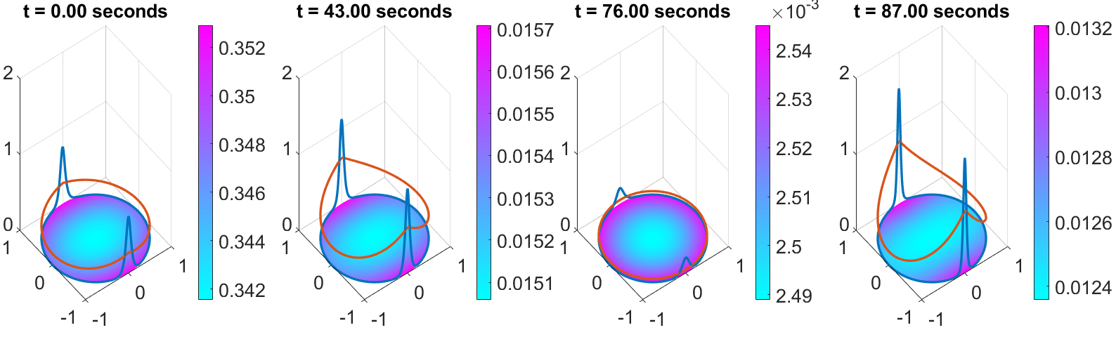
Figure 2: Snapshots of the numerically computed solution of (1.1) starting from a 2-spike equilibrium for the unit disk with $D_{b}=10$, $\tau_{s}=0.6$, $\tau_{b}=0.1$, $K=0.025$, and $D_{v}=1.8$ (this corresponds to point $5$ in the left panel of Figure 13). The bulk inhibitor is shown as the colourmap, whereas the lines along the boundary indicate the activator (blue) and inhibitor (orange) membrane concentrations. The results show a synchronous oscillatory instability of the spike amplitudes.

As an illustration of spike dynamics resulting from full PDE simulations, in Figures 1 and 2 we show results computed for the unit disk with $D_{b}=10$, showing competition and oscillatory instabilities for a two-spike solution, respectively. The parameter values are given in the figure captions and correspond to specific points in the linear stability phase diagram given in the left panel of Figure 13.

In §4 we use a regular perturbation analysis to show the effect on the asynchronous instability thresholds of introducing a small smooth perturbation of the boundary of the unit disk. This analysis, which requires a detailed calculation of the perturbed 1-D membrane Green’s function, shows that a two-spike pattern can be stabilized by a small outward peanut-shaped deformation of a circular disk. Finally, in §5 we briefly summarize our results and highlight some open problems and directions for future research.

2 Spike Equilibrium and its Linear Stability: General Asymptotic Theory

2.1 Asymptotic Construction of $N$-Spike Equilibria

In this section we provide an asymptotic construction of an $N$-spike steady-state solution to (1.1). Specifically, we consider the steady-state problem for the membrane species

$$\varepsilon^{2}\partial_{\sigma}^{2}u_{e}-u_{e}+u_{e}^{p}/v_{e}^{q}=0\,,\qquad 0<\sigma<L\,,\quad u\,\,\mbox{is $L$-periodic}\,,$$ (2.1a)

$$D_{v}\partial_{\sigma}^{2}v_{e}-(1+K)v_{e}+KV_{e}+\varepsilon^{-1}u_{e}^{m}/v_{e}^{s}=0\,,\qquad 0<\sigma<L\,,\quad v\,\,\mbox{is $L$-periodic}\,,$$ (2.1b)

which is coupled to the steady-state bulk-diffusion process by

$$D_{b}\Delta V_{e}-V_{e}=0\,,\quad x\in\Omega\,;\qquad D_{b}\partial_{n}V_{e}+KV_{e}=Kv_{e}\,,\quad x\in\partial\Omega\,.$$ (2.1c)

From (2.1c), the bulk-inhibitor evaluated on the membrane is readily expressed in terms of a Green’s function as

$$V_{e}(\sigma)=K\int_{0}^{L}G_{\Omega}(\sigma,\tilde{\sigma})v_{e}(\tilde{\sigma})\,d\tilde{\sigma}\,,$$ (2.2)

where we have used arc-length to parameterize the boundary. Here, $G_{\Omega}(\sigma,\tilde{\sigma})$ is the Green’s function satisfying

$$D_{b}\Delta_{x}G_{\Omega}(x,\tilde{\sigma})-G_{\Omega}(x,\tilde{\sigma})=0\,,\quad x\in\Omega\,,\qquad D_{b}\partial_{n}G_{\Omega}(\sigma,\tilde{\sigma})+KG_{\Omega}(\sigma,\tilde{\sigma})=\delta(\sigma-\tilde{\sigma})\,,\quad 0<\sigma<L\,.$$ (2.3)

We remark that the values of the bulk-inhibitor field within the bulk can likewise be obtained with a Green’s function whose source is in the interior. However, for our purposes it is only the restriction to the boundary that is important.

At this stage the steady-state membrane problem takes the form

$$\begin{split}\varepsilon^{2}\partial_{\sigma}^{2}u_{e}-u_{e}+&u_{e}^{p}/v_{e}^{q}=0\,,\qquad 0<\sigma<L\,,\\ D_{v}\partial_{\sigma}^{2}v_{e}-(1+K)v_{e}+&K^{2}\int_{0}^{L}G_{\Omega}(\sigma,\tilde{\sigma})v_{e}(\tilde{\sigma})\,d\tilde{\sigma}+\varepsilon^{-1}u_{e}^{m}/v_{e}^{s}=0\,,\qquad 0<\sigma<L\,,\end{split}$$ (2.4)

which differs from the problem studied in [8] for the uncoupled ($K=0$) case only by the addition of the non-local term. This additional term leads to difficulties in the construction of spike patterns. In particular, it complicates the concept of a "symmetric" pattern since, in general, the non-local term will not be translation invariant. Moreover, in the well-mixed and disk case, the construction of asymmetric patterns is more intricate as a result of the non-local term.

We now construct an $N$-spike steady-state pattern for (2.4) characterized by an activator concentration that is localized at $N$ distinct spike locations $0\leq\sigma_{1}<...<\sigma_{N}<L$ to be determined. We assume that the spikes are well-separated in the sense that $|\sigma_{\{{(i+1)\mod N\}}}-\sigma_{i}\mod L|\gg\varepsilon$ for $i=1,\ldots,N$. Upon introducing stretched coordinates $y=\varepsilon^{-1}(\sigma-\sigma_{j})$, we deduce that the inhibitor field is asymptotically constant near each spike, i. e.

$$v_{e}\sim v_{ej}\equiv v_{e}(\sigma_{j})\,.$$ (2.5)

In addition, the activator concentration is determined in terms of the unique solution $w(y)$ to the core problem

$$w^{\prime\prime}-w+w^{p}=0\,,\quad y\in\mathbb{R}\,,\qquad w^{\prime}(0)=0\,,\quad w(0)>0\,,\quad w(y)\rightarrow 0\quad\mbox{as}\quad|y|\rightarrow\infty\,.$$ (2.6)

Since the solution to the core problem decays exponentially as $y\rightarrow\pm\infty$ we deduce that

$$u_{e}(\sigma)\sim\sum_{j=1}^{N}v_{ej}^{\gamma}w\bigl{(}\varepsilon^{-1}[\sigma-\sigma_{j}]\bigr{)}\,,\qquad\mbox{as}\quad\varepsilon\rightarrow 0\,,$$ (2.7)

where $\gamma\equiv q/(p-1)$. The solution to (2.6) is given explicitly as

$$w(y)=\biggl{(}\frac{p+1}{2}\biggr{)}^{\frac{1}{p-1}}\biggl{[}\text{sech}\biggl{(}\frac{p-1}{2}y\biggr{)}\biggr{]}^{\frac{2}{p-1}}.$$ (2.8)

Next, since $u_{e}$ is localized, we have in the sense of distributions that

$$\varepsilon^{-1}u_{e}^{m}/v_{e}^{s}\longrightarrow\omega_{m}\sum_{j=1}^{N}[v_{e}(\sigma_{j})]^{\gamma m-s}\delta(\sigma-\sigma_{j})\qquad\mbox{as}\quad\varepsilon\rightarrow 0\,,$$

where we have defined

$$\omega_{m}\equiv\int_{-\infty}^{\infty}[w(y)]^{m}\,dy\,.$$ (2.9)

In this way, for $\varepsilon\rightarrow 0$, we obtain from (2.4) the following integro-differential equation for the inhibitor field:

$$D_{v}\partial_{\sigma}^{2}v_{e}-(1+K)v_{e}+K^{2}\int_{0}^{L}G_{\Omega}(\sigma,\tilde{\sigma})v_{e}(\tilde{\sigma})\,d\tilde{\sigma}=-\omega_{m}\sum_{j=1}^{N}v_{ej}^{\gamma m-s}\delta(\sigma-\sigma_{j})\,.$$ (2.10)

To conveniently represent the solution to this equation we introduce the Green’s function $G_{\partial\Omega}(\sigma,\zeta)$ satisfying

$$D_{v}\partial_{\sigma}^{2}G_{\partial\Omega}(\sigma,\zeta)-(1+K)G_{\partial\Omega}(\sigma,\zeta)+K^{2}\int_{0}^{L}G_{\Omega}(\sigma,\tilde{\sigma})G_{\partial\Omega}(\tilde{\sigma},\zeta)\,d\tilde{\sigma}=-\delta(\sigma-\zeta)\,,\qquad 0<\sigma,\zeta<L\,.$$ (2.11)

In terms of this Green’s function, the membrane inhibitor field is given by

$$v_{e}(\sigma)=\omega_{m}\sum_{j=1}^{N}v_{ej}^{\gamma m-s}G_{\partial\Omega}(\sigma,\sigma_{j})\,.$$ (2.12)

Substituting $\sigma=\sigma_{i}$, and recalling the definition $v_{ei}\equiv v_{e}(\sigma_{i})$, (2.12) yields the $N$ self-consistency conditions

$$v_{ei}-\omega_{m}\sum_{j=1}^{N}v_{ej}^{\gamma m-s}G_{\partial\Omega}(\sigma_{i},\sigma_{j})=0\,,\qquad i=1,\ldots,N\,.$$ (2.13)

These conditions provide the first $N$ algebraic equations for our overall system in $2N$ unknowns to be completed below. The remaining $N$ equations arise from solvability conditions when performing a higher-order matched asymptotic expansion analysis of the steady-state solution.

To this end, we again introduce stretched coordinates $y=\varepsilon^{-1}\bigl{(}\sigma-\sigma_{j})$, but we now introduce a two-term inner expansion for the surface bound species for $\varepsilon\to 0$ as

$$u_{e}(y)\sim v_{ej}^{\gamma}w(y)+\varepsilon u_{1}(y)+{\mathcal{O}}(\varepsilon^{2})\,,\qquad v_{e}(y)\sim v_{ej}+\varepsilon v_{1}(y)+{\mathcal{O}}(\varepsilon^{2})\,,\qquad V_{e}\sim{\mathcal{O}}(1)\,.$$ (2.14)

Upon substituting this expansion into (2.1), and collecting the ${\mathcal{O}}(\varepsilon)$ terms, we get

$$\mathcal{L}_{0}u_{1}\equiv u_{1}^{\prime\prime}-u_{1}+pw^{p-1}u_{1}=qv_{ej}^{\gamma-1}w^{p}v_{1}\,,\qquad D_{v}v_{1}^{\prime\prime}+v_{ej}^{\gamma m-s}w^{m}=0\,.$$ (2.15)

Since $\mathcal{L}_{0}w^{\prime}=0$, the solvability condition for the first equation yields that

$$qv_{ej}^{\gamma-1}\int_{-\infty}^{\infty}w^{p}w^{\prime}v_{1}\,dy=0\qquad\Longleftrightarrow\qquad\int_{-\infty}^{\infty}(w^{p+1})^{\prime}v_{1}\,dy=0\,.$$

Then, we integrate by parts twice, use the exponential decay of $w(y)$ as $|y|\rightarrow\infty$, and substitute (2.15) for $v_{1}^{\prime\prime}$. This yields that

$$I_{p}(y)v_{1}^{\prime}(y)\biggr{|}_{-\infty}^{\infty}+\frac{v_{ej}^{\gamma m-s}}{D_{v}}\int_{-\infty}^{\infty}I_{p}(y)[w(y)]^{m}\,dy=0\,,$$

where we have defined $I_{p}(y)\equiv\int_{0}^{y}[w(z)]^{p+1}dz$. Since $w$ is even, while $I_{p}$ is odd, the integral above vanishes, and we get

$$v_{1}^{\prime}(+\infty)+v_{1}^{\prime}(-\infty)=0\,.$$

In this way, a higher order matching process between the inner and outer solutions yields the balance conditions,

$$\partial_{\sigma}v_{e}(\sigma_{i}+0)+\partial_{\sigma}v_{e}(\sigma_{i}-0)=0\,,\qquad i=1,\ldots,N\,.$$

By using (2.12) for $v_{e}$, we can write these balance equations in terms of the Green’s function $G_{\partial\Omega}$ as

$$v_{ei}^{\gamma m-s}\bigl{[}\partial_{\sigma}G_{\partial\Omega}(\sigma_{i}+0,\sigma_{i})+\partial_{\sigma}G_{\partial\Omega}(\sigma_{i}-0,\sigma_{i})\bigr{]}+2\sum_{j\neq i}v_{ej}^{\gamma m-s}\partial_{\sigma}G_{\partial\Omega}(\sigma_{i},\sigma_{j})=0\,,\qquad i=1,\ldots,N\,.$$ (2.16)

We summarize the results of this formal asymptotic construction in the following proposition:

Proposition 2.1

As $\varepsilon\rightarrow 0$ an $N$-spike steady-state solution to (2.1) with spikes centred at $\sigma_{1},...,\sigma_{N}$ is asymptotically given by

$$u_{e}(\sigma)\sim\sum_{j=1}^{N}v_{ej}^{\gamma}w\bigl{(}\varepsilon^{-1}[\sigma-\sigma_{j}])\,,\qquad v_{e}(\sigma)\sim\omega_{m}\sum_{j=1}^{N}v_{ej}^{\gamma m-s}G_{\partial\Omega}(\sigma,\sigma_{j})\,,$$ (2.17a)

$$V_{e}(\sigma)\sim\omega_{m}K\sum_{j=1}^{N}v_{ej}^{\gamma m-s}\int_{0}^{L}G_{\Omega}(\sigma,\tilde{\sigma})G_{\partial\Omega}(\tilde{\sigma},\sigma_{j})\,d\tilde{\sigma}\,,$$ (2.17b)

where $\omega_{m}\equiv\int_{-\infty}^{\infty}[w(y)]^{m}\,dy$ and $\gamma\equiv{q/(p-1)}$. Here the steady-state spike locations $\sigma_{1},...,\sigma_{N}$ and $v_{e1},...,v_{eN}$, which determine the heights of the spikes, are to be found from the following non-linear algebraic system:

$$v_{ei}-\omega_{m}\sum_{j=1}^{N}v_{ej}^{\gamma m-s}G_{\partial\Omega}(\sigma_{i},\sigma_{j})=0\,,\qquad i=1,\ldots,N\,,$$ (2.18a)

$$v_{ei}^{\gamma m-s}\bigl{[}\partial_{\sigma}G_{\partial\Omega}(\sigma_{i}+0,\sigma_{i})+\partial_{\sigma}G_{\partial\Omega}(\sigma_{i}-0,\sigma_{i})\bigr{]}+2\sum_{j\neq i}v_{ej}^{\gamma m-s}\partial_{\sigma}G_{\partial\Omega}(\sigma_{i},\sigma_{j})=0\,,\qquad i=1,\ldots,N\,.$$ (2.18b)

2.2 Linear Stability of $N$-Spike Equilibria

In our linear stability analysis, given below, of $N$-spike equilibria we make two simplifying assumptions. First, we focus exclusively on the case $s=0$. Second, we consider only instabilities that arise on an ${\mathcal{O}}(1)$ timescale. Therefore, we do not consider very weak instabilities, occurring on asymptotically long time-scales in $\varepsilon$, that are due to any unstable small eigenvalue that tends to zero as $\varepsilon\to 0$.

Let $u_{e}(\sigma)$, $v_{e}(\sigma)$, and $V_{e}(x)$ denote the the steady-state constructed in §2.1. For $\lambda\in\mathbb{C}$, we consider a perturbation of the form

$$u(\sigma)=u_{e}(\sigma)+e^{\lambda t}\phi(\sigma)\,,\qquad v(\sigma)=v_{e}(\sigma)+e^{\lambda t}\psi(\sigma)\,,\qquad V(x)=V_{e}(x)+e^{\lambda t}\eta(x)\,,$$

where $\phi$, $\psi$, and $\eta$ are small. Upon substituting into (1.1) and linearizing, we obtain the eigenvalue problem

$$\varepsilon^{2}\partial_{\sigma}^{2}\phi-\phi+pu_{e}^{p-1}v_{e}^{-q}\phi-qu_{e}^{p}v_{e}^{-(q+1)}\psi=\lambda\phi\,,\qquad 0<\sigma<L\,,$$ (2.19a)

$$D_{v}\partial_{\sigma}^{2}\psi-\mu_{s\lambda}^{2}\psi+K\eta=-m\varepsilon^{-1}u_{e}^{m-1}\phi\,,\qquad 0<\sigma<L\,,$$ (2.19b)

$$D_{b}\Delta\eta-\mu_{b\lambda}^{2}\eta=0\,,\qquad x\in\Omega\,,$$ (2.19c)

$$D_{b}\partial_{n}\eta+K\eta=K\psi\,,\qquad x\in\partial\Omega\,,$$ (2.19d)

where we have defined $\mu_{s\lambda}$ and $\mu_{b\lambda}$ by

$$\mu_{s\lambda}=\sqrt{1+K+\tau_{s}\lambda}\,,\qquad\mu_{b\lambda}=\sqrt{1+\tau_{b}\lambda}\,.$$ (2.20)

The bulk inhibitor field evaluated on the boundary is represented as

$$\eta(\sigma)=K\int_{0}^{L}G^{\lambda}_{\Omega}(\sigma,\tilde{\sigma})\psi(\tilde{\sigma})\,d\tilde{\sigma}\,,$$

where $G^{\lambda}_{\Omega}$ is the $\lambda$-dependent bulk Green’s function satisfying

$$D_{b}\Delta_{x}G_{\Omega}^{\lambda}(x,\tilde{\sigma})-\mu_{b\lambda}^{2}G_{\Omega}^{\lambda}(x,\tilde{\sigma})=0\,,\quad x\in\Omega\,,\qquad D_{b}\partial_{n}G_{\Omega}^{\lambda}(\sigma,\tilde{\sigma})+KG_{\Omega}^{\lambda}(\sigma,\tilde{\sigma})=\delta(\sigma-\tilde{\sigma})\,,\quad 0<\sigma<L\,.$$ (2.21)

Next, we seek a localized activator perturbation of the form

$$\phi(\sigma)\sim\sum_{j=1}^{N}\phi_{j}\bigl{(}\varepsilon^{-1}[\sigma-\sigma_{j}]\bigr{)}\,,$$ (2.22)

where we impose that $\phi_{j}(y)\rightarrow 0$ as $|y|\rightarrow\infty$. With this form, we evaluate in the sense of distributions that

$$\varepsilon^{-1}mu_{e}^{m-1}\phi\longrightarrow m\sum_{j=1}^{N}v_{ej}^{\gamma(m-1)}\left(\int_{-\infty}^{\infty}[w(y)]^{m-1}\phi_{j}(y)\,dy\right)\,\delta(\sigma-\sigma_{j})\qquad\mbox{as}\quad\varepsilon\rightarrow 0\,.$$

By using this limiting result in (2.19b), the problem for $\psi$ becomes

$$D_{v}\partial_{\sigma}^{2}\psi-\mu_{s\lambda}^{2}\psi+K^{2}\int_{0}^{L}G_{\Omega}^{\lambda}(\sigma,\tilde{\sigma})\psi(\tilde{\sigma})\,d\tilde{\sigma}=-m\sum_{j=1}^{N}v_{ej}^{\gamma(m-1)}\left(\int_{-\infty}^{\infty}[w(y)]^{m-1}\phi_{j}(y)\,dy\right)\,\delta(\sigma-\sigma_{j})\,.$$

The solution to this problem is represented as

$$\psi(\sigma)=m\sum_{j=1}^{N}v_{ej}^{\gamma(m-1)}G_{\partial\Omega}^{\lambda}(\sigma,\sigma_{j})\int_{-\infty}^{\infty}[w(y)]^{m-1}\phi_{j}(y)\,dy\,,$$ (2.23)

where $G_{\partial\Omega}^{\lambda}$ is the $\lambda$-dependent membrane Green’s function satisfying

$$D_{v}\partial_{\sigma}^{2}G_{\partial\Omega}^{\lambda}(\sigma,\zeta)-\mu_{s\lambda}^{2}G_{\partial\Omega}^{\lambda}(\sigma,\zeta)+K^{2}\int_{0}^{L}G_{\Omega}^{\lambda}(\sigma,\tilde{\sigma})G_{\partial\Omega}^{\lambda}(\tilde{\sigma},\zeta)\,d\tilde{\sigma}=-\delta(\sigma-\zeta)\,,\qquad 0<\sigma,\zeta<L\,.$$ (2.24)

Next, it is convenient to re-scale $v_{e}$ as

$$v_{e}(\sigma)=\omega_{m}^{\frac{1}{1-\gamma m}}\hat{v}_{e}(\sigma)\,,\qquad v_{ej}=\omega_{m}^{\frac{1}{1-\gamma m}}\hat{v}_{ej}\,.$$ (2.25)

In the stretched coordinates $y=\varepsilon^{-1}(\sigma-\sigma_{j})$, we use (2.23) to obtain that (2.19a) becomes

$$\phi_{i}^{\prime\prime}-\phi_{i}+pw^{p-1}\phi_{i}-mqw^{p}\sum_{j=1}^{N}\hat{v}_{ei}^{\gamma-1}G_{\partial\Omega}^{\lambda}(\sigma_{i},\sigma_{j})\hat{v}_{ej}^{\gamma(m-1)}\frac{\int_{-\infty}^{\infty}w^{m-1}\phi_{j}\,dy}{\int_{-\infty}^{\infty}w^{m}\,dy}=\lambda\phi_{i}\,.$$

To recast this spectral problem in vector form we define

$$\boldsymbol{\phi}\equiv\begin{pmatrix}\phi_{1}\\ \vdots\\ \phi_{N}\end{pmatrix}\,,\quad\hat{\mathcal{V}}_{e}\equiv\begin{pmatrix}\hat{v}_{e1}&&0\\ &\ddots&\\ 0&&\hat{v}_{eN}\end{pmatrix}\,,\quad\mathcal{G}_{\partial\Omega}^{\lambda}\equiv\begin{pmatrix}G_{\partial\Omega}^{\lambda}(\sigma_{1},\sigma_{1})&\cdots&G_{\partial\Omega}^{\lambda}(\sigma_{1},\sigma_{N})\\ \cdots&\ddots&\vdots\\ G_{\partial\Omega}^{\lambda}(\sigma_{N},\sigma_{1})&\cdots&G_{\partial\Omega}^{\lambda}(\sigma_{N},\sigma_{N})\end{pmatrix}\,,$$ (2.26)

and we introduce the matrix $\mathcal{E}$ by

$$\mathcal{E}\equiv\hat{\mathcal{V}}_{e}^{\gamma-1}\mathcal{G}_{\partial\Omega}^{\lambda}\hat{\mathcal{V}}_{e}^{\gamma(m-1)}\,.$$ (2.27)

In this way, we deduce that $\boldsymbol{\phi}$ must solve the vector nonlocal eigenvalue problem (NLEP) given by

$$\boldsymbol{\phi}^{\prime\prime}(y)-\boldsymbol{\phi}(y)+pw^{p-1}\boldsymbol{\phi}(y)-mqw^{p}\frac{\int_{-\infty}^{\infty}[w(y)]^{m-1}\mathcal{E}\boldsymbol{\phi}(y)\,dy}{\int_{-\infty}^{\infty}[w(y)]^{m}\,dy}=\lambda\boldsymbol{\phi}(y)\,.$$ (2.28)

We can reduce this vector NLEP to a collection of scalar NLEPs by diagonalizing it. Specifically, we seek perturbations of the form $\boldsymbol{\phi}=\phi\boldsymbol{c}$ where $\boldsymbol{c}$ is an eigenvector of $\mathcal{E}$, that is

$$\mathcal{E}\boldsymbol{c}=\chi(\lambda)\boldsymbol{c}\,.$$ (2.29)

Then, it readily follows that the vector NLEP (2.28) can be recast as the scalar NLEP

$$\mathcal{L}_{0}\phi-mq\chi(\lambda)w^{p}\frac{\int_{-\infty}^{\infty}[w(y)]^{m-1}\phi(y)\,dy}{\int_{-\infty}^{\infty}[w(y)]^{m}\,dy}=\lambda\phi\,,$$ (2.30)

where $\chi(\lambda)$ is any eigenvalue of $\mathcal{E}$. In (2.30), the operator $\mathcal{L}_{0}$, referred to as the local operator, is defined by

$$\mathcal{L}_{0}\phi\equiv\phi^{\prime\prime}(y)-\phi(y)+pw^{p-1}\phi(y)\,.$$ (2.31)

Notice that we obtain a (possibly) different NLEP for each eigenvalue $\chi(\lambda)$ of $\mathcal{E}$. Therefore, the spectrum of the matrix $\mathcal{E}$ will be central in the analysis below for classifying the various types of instabilities that can occur.

2.3 Reduction of NLEP to an Algebraic Equation and an Explicitly Solvable Case

Next, we show how to reduce the determination of the spectrum of the NLEP (2.30) to a root-finding problem. To this end, we define $c_{m}$ by

$$c_{m}\equiv mq\chi(\lambda)\frac{\int_{-\infty}^{\infty}[w(y)]^{m-1}\phi(y)\,dy}{\int_{-\infty}^{\infty}[w(y)]^{m}\,dy}\,,$$ (2.32)

and write the NLEP as $(\mathcal{L}_{0}-\lambda)\phi=c_{m}w^{p}$, so that $\phi=c_{m}(\mathcal{L}_{0}-\lambda)^{-1}w^{p}$. Upon multiplying both sides of this expression by $w^{m-1}$, we integrate over the real line and substitute the resulting expression back into (2.32). For eigenfunctions for which $\int_{-\infty}^{\infty}w^{m-1}\phi\,dy\neq 0$, we readily obtain that $\lambda$ must be a root of $\mathcal{A}(\lambda)=0$, where

$$\mathcal{A}(\lambda)\equiv\mathcal{C}(\lambda)-\mathcal{F}(\lambda)\qquad\mathcal{C}\equiv\frac{1}{\chi(\lambda)}\,,\qquad\mathcal{F}(\lambda)\equiv mq\frac{\int_{-\infty}^{\infty}[w(y)]^{m-1}(\mathcal{L}_{0}-\lambda)^{-1}[w(y)]^{p}\,dy}{\int_{-\infty}^{\infty}[w(y)]^{m}\,dy}\,.$$ (2.33)

Since, it is readily shown that there are no unstable eigenvalues of the NLEP (2.30) for eigenfunctions for which $\int_{-\infty}^{\infty}w^{m-1}\phi\,dy=0$, the roots of $\mathcal{A}(\lambda)=0$ will provide all the unstable eigenvalues of the NLEP (2.30).

For general Gierer-Meinhardt exponents, the spectral theory of the operator $\mathcal{L}_{0}$ leads to some detailed properties of the term $\mathcal{F}(\lambda)$ for various exponent sets (cf. [20]). In addition, to make further progress on the root-finding problem (2.33), we need some explicit results for the multiplier $\chi(\lambda)$.

For special sets of Gierer-Meinhardt exponents, known as the “explicitly solvable cases” (cf. [13]), the term $\mathcal{F}(\lambda)$ can be evaluated explicitly. We focus specifically on one such set $(p,q,m,0)=(3,1,3,0)$ for which the key identity $\mathcal{L}_{0}w^{2}=3w^{2}$ holds, where $w=\sqrt{2}\,\mbox{sech}{y}$ from (2.8). Thus, after integrating by parts we obtain

$$\int_{-\infty}^{\infty}w^{2}(\mathcal{L}_{0}-\lambda)^{-1}w^{3}dy=\frac{\int_{-\infty}^{\infty}(\mathcal{L}_{0}-\lambda)w^{2}(\mathcal{L}_{0}-\lambda)^{-1}w^{3}dy}{3-\lambda}=\frac{\int_{-\infty}^{\infty}w^{2}(\mathcal{L}_{0}-\lambda)(\mathcal{L}_{0}-\lambda)^{-1}w^{3}dy}{3-\lambda}=\frac{\int_{-\infty}^{\infty}w^{5}dy}{3-\lambda}.$$

By making use of the identities

$$\int_{-\infty}^{\infty}w^{5}dy=\dfrac{3\pi}{\sqrt{2}},\qquad\int_{-\infty}^{\infty}w^{3}dy=\sqrt{2}\pi,$$

we obtain that $\mathcal{F}(\lambda)={9/\left[2(3-\lambda)\right]}$, so that the root-finding problem (2.33) reduces to determining $\lambda$ such that

$$\mathcal{A}(\lambda)\equiv\frac{1}{\chi(\lambda)}-\frac{9/2}{3-\lambda}=0\,.$$ (2.34)

In addition to the explicitly solvable case $(p,q,m,s)=(3,1,3,0)$, the root-finding problem (2.33) simplifies considerably for a general Gierer-Meinhardt exponent set, when we focus on determining parameter thresholds for zero-eigenvalue crossings (corresponding to asynchronous instabilities). Since $\mathcal{L}_{0}w=w^{\prime\prime}-w+pw^{p}=(p-1)w^{p}$, it follows that $\mathcal{L}_{0}^{-1}w^{p}=\tfrac{1}{p-1}w$, from which we calculate

$$\mathcal{F}(0)=mq\frac{\int_{-\infty}^{\infty}w^{m-1}\mathcal{L}_{0}^{-1}w^{p}\,dy}{\int_{-\infty}^{\infty}w^{m}\,dy}=\frac{mq}{p-1}\,.$$

Therefore, a zero-eigenvalue crossing for a general Gierer-Meinhardt exponent set occurs when

$$\mathcal{A}(0)=\frac{1}{\chi(0)}-\frac{mq}{p-1}=0\,.$$ (2.35)

3 Symmetric $N$-Spike Patterns: Equilibria and Stability

For the remainder of this paper we will focus exclusively on symmetric $N$-spike steady-states that are characterized by equidistant (in arc-length) spikes of equal heights. Due to the bulk-membrane coupling it is unclear whether such symmetric patterns will exist for a general domain. Indeed it may be that a spike pattern with spikes of equal heights may require the equidistant requirement to be dropped. These more general considerations can perhaps be better approached by requiring that a certain Green’s matrix admit the eigenvector $\mathbf{e}=(1,...,1)^{T}$.

Avoiding these additional complications, we focus instead on two distinct cases for which symmetric spike patterns, as we have defined them, can be constructed. The first case is the disk of radius $R$, denoted by $\Omega=B_{R}(0)$, and the second case corresponds to the well-mixed limit for which $D_{b}\rightarrow\infty$ in an arbitrary bounded domain. In both cases the Green’s function is invariant under translations, satisfying

$$G_{\partial\Omega}(\sigma+\vartheta\mod L,\zeta+\vartheta\mod L)=G_{\partial\Omega}(\sigma,\zeta)\,,\qquad\forall\,\,\sigma\,,\zeta\in[0,L)\,,\qquad\vartheta\in\mathbb{R}\,.$$

By using this key property in (2.18a), we calculate the common spike height as

$$v_{ej}=v_{e0}=\biggl{[}\omega_{m}\sum_{k=0}^{N-1}G_{\partial\Omega}\biggl{(}\frac{kL}{N},0\biggr{)}\biggr{]}^{\frac{1}{1-\gamma m+s}}\,.$$ (3.1)

With a common spike height, the balance equations (2.18b) then reduce to

$$\bigl{[}\partial_{\sigma}G_{\partial\Omega}(0^{+},0)+\partial_{\sigma}G_{\partial\Omega}(0^{-},0)\bigr{]}+2\sum_{k=1}^{N-1}\partial_{\sigma}G_{\partial\Omega}\biggl{(}\frac{kL}{N},0\biggr{)}=0\,,$$ (3.2)

which can be verified either explicitly or by using the symmetry of the Green’s function.

For a symmetric $N$-spike steady-state the NLEP (2.30) can be simplified significantly. First the matrix $\mathcal{E}$, defined in (2.27), simplifies to

$$\mathcal{E}=\hat{v}_{e0}^{\gamma m-1}\mathcal{G}_{\partial\Omega}^{\lambda}\,.$$

Therefore, from (2.29) it follows that $\chi(\lambda)=\hat{v}_{e0}^{\gamma m-1}\mu(\lambda)$, where $\mu(\lambda)$ is an eigenvalue of the Green’s matrix $\mathcal{G}_{\partial\Omega}^{\lambda}$ defined in (2.26). Furthermore, by using the bi-translation invariance and symmetry of $G_{\partial\Omega}^{\lambda}$, we can define

$$H_{|j-i|}^{\lambda}\equiv G_{\partial\Omega}^{\lambda}(|\sigma_{i}-\sigma_{j}|,0)=G_{\partial\Omega}^{\lambda}(|i-j|L/N,0)\,,$$ (3.3)

which allows us to write the Green’s matrix as

$$\mathcal{G}_{\partial\Omega}^{\lambda}=\begin{pmatrix}H_{0}^{\lambda}&H_{1}^{\lambda}&H_{2}^{\lambda}&\cdots&H_{N-1}^{\lambda}\\ H_{N-1}^{\lambda}&H_{0}^{\lambda}&H_{1}^{\lambda}&\cdots&H_{N-2}^{\lambda}\\ \vdots&\vdots&\vdots&\ddots&\vdots\\ H_{1}^{\lambda}&H_{2}^{\lambda}&H_{3}^{\lambda}&\cdots&H_{0}^{\lambda}\end{pmatrix}\,,$$

which we recognize as a circulant matrix. As a result, the matrix spectrum of $\mathcal{G}_{\partial\Omega}^{\lambda}$ is readily available as

$$\mu_{k}(\lambda)=\sum_{j=0}^{N-1}H_{j}^{\lambda}e^{i\frac{2\pi jk}{N}}\,,\qquad\boldsymbol{c}_{k}(\lambda)=\biggl{(}1,\cdots,e^{i\frac{2\pi(N-1)k}{N}}\biggr{)}^{T}\,,\qquad k=0,\ldots,N-1\,.$$ (3.4)

For each value of $k=0,\ldots,N-1$ we obtain a corresponding NLEP problem from (2.30). Since $\boldsymbol{c}_{0}=(1,\ldots,1)^{T}$ we can interpret this “mode” as a synchronous perturbation. In contrast, the values $k=1,\ldots,N-1$ for $N\geq 2$ correspond to asynchronous perturbations, since the corresponding eigenvectors $\boldsymbol{c}_{k}(\lambda)$ are all orthogonal to $(1,\ldots,1)^{T}$. Any unstable asynchronous “mode” of this type is referred to as a competition instability, in the sense that the linear stability theory predicts that the heights of individual spikes may grow or decay, but that the overall sum of all the spike heights remains fixed. For each value of $k$, the NLEP (2.30) becomes

$$\mathcal{L}_{0}\phi-mq\chi_{k}(\lambda)w^{p}\dfrac{\int_{-\infty}^{\infty}[w(y)]^{m-1}\phi(y)\,dy}{\int_{-\infty}^{\infty}[w(y)]^{m}\,dy}=\lambda\phi\,,\qquad\mbox{where}\quad\chi_{k}(\lambda)\equiv\frac{\mu_{k}(\lambda)}{\sum_{j=1}^{N-1}G_{\partial\Omega}(jL/N,0)}=\frac{\mu_{k}(\lambda)}{\mu_{0}(0)}\,.$$ (3.5)

Further analysis requires details of the Green’s function $G_{\partial\Omega}^{\lambda}$, which are available in our two special cases.

3.1 NLEP Multipliers for the Well-Mixed Limit

In the well-mixed limit, $D_{b}\to\infty$, the membrane Green’s function, satisfying (2.24), is given by (see (A.5) of Appendix A)

$$G_{\partial\Omega}^{\lambda}(\sigma,\zeta)=\Gamma^{\lambda}(|\sigma-\zeta|)+\frac{K^{2}}{\mu_{s\lambda}^{2}A}\frac{1}{\mu_{s\lambda}^{2}(\mu_{b\lambda}^{2}+\beta)-K\beta}=\Gamma^{\lambda}(|\sigma-\zeta|)+\frac{\gamma_{\lambda}}{\mu_{s\lambda}^{2}}\,,\quad\gamma_{\lambda}\equiv\frac{K^{2}/A}{\mu_{s\lambda}^{2}(\mu_{b\lambda}^{2}+\beta)-K\beta}\,,$$ (3.6)

where $\beta\equiv{KL/A}$. Here $\Gamma^{\lambda}$ is the periodic Green’s function for the uncoupled ($K=0$) problem, which is given explicitly by (A.2) of Appendix A as

$$\Gamma^{\lambda}(x)=\frac{1}{2\sqrt{D_{v}}\mu_{s\lambda}}\coth\biggl{(}\frac{\mu_{s\lambda}L}{2\sqrt{D_{v}}}\biggr{)}\cosh\biggl{(}\frac{\mu_{s\lambda}}{\sqrt{D_{v}}}|x|\biggr{)}-\frac{1}{2\sqrt{D_{v}}\mu_{s\lambda}}\sinh\biggl{(}\frac{\mu_{s\lambda}}{\sqrt{D_{v}}}|x|\biggr{)}\,.$$

After some algebra we use (3.4) to calculate the eigenvalues $\mu_{k}(\lambda)$ of the Green’s matrix as

$$\mu_{k}(\lambda)=\sum_{j=0}^{N-1}\Gamma^{\lambda}(jL/n)e^{i\frac{2\pi jk}{N}}+\delta_{k0}\frac{N\gamma_{\lambda}}{\mu_{s\lambda}^{2}}=\frac{1}{2\sqrt{D_{v}}\mu_{s\lambda}}\frac{\cosh\bigl{(}\frac{\mu_{s\lambda}L}{2N\sqrt{D_{v}}}\bigr{)}\sinh\bigl{(}\frac{\mu_{s\lambda}L}{2N\sqrt{D_{v}}}\bigr{)}}{\sinh\bigl{(}\frac{\mu_{s\lambda}L}{2N\sqrt{D_{v}}}+\frac{i\pi k}{N}\bigr{)}\sinh\bigl{(}\frac{\mu_{s\lambda}L}{2N\sqrt{D_{v}}}-\frac{i\pi k}{N}\bigr{)}}+\delta_{k0}\frac{N\gamma_{\lambda}}{\mu_{s\lambda}^{2}}\,,$$

where $\delta_{k0}$ is the Kronecker symbol. In this way, we obtain from (3.5) that the NLEP multipliers are given by

$$\chi_{0}(\lambda)=\frac{\frac{1}{2\sqrt{D_{v}}\mu_{s\lambda}}\coth\biggl{(}\frac{\mu_{s\lambda}L}{2N\sqrt{D_{v}}}\biggr{)}+\frac{N\gamma_{\lambda}}{\mu_{s\lambda}^{2}}}{\frac{1}{2\sqrt{D_{v}}\mu_{s0}}\coth\biggl{(}\frac{\mu_{s0}L}{2N\sqrt{D_{v}}}\biggr{)}+\frac{N\gamma_{0}}{\mu_{s0}^{2}}}\,,\qquad\chi_{k}(\lambda)=\frac{\frac{1}{2\sqrt{D_{v}}\mu_{s\lambda}}\frac{\cosh\bigl{(}\frac{\mu_{s\lambda}L}{2N\sqrt{D_{v}}}\bigr{)}\sinh\bigl{(}\frac{\mu_{s\lambda}L}{2N\sqrt{D_{v}}}\bigr{)}}{\sinh\bigl{(}\frac{\mu_{s\lambda}L}{2N\sqrt{D_{v}}}+\frac{i\pi k}{N}\bigr{)}\sinh\bigl{(}\frac{\mu_{s\lambda}L}{2N\sqrt{D_{v}}}-\frac{i\pi k}{N}\bigr{)}}}{\frac{1}{2\sqrt{D_{v}}\mu_{s0}}\coth\biggl{(}\frac{\mu_{s0}L}{2N\sqrt{D_{v}}}\biggr{)}+\frac{N\gamma_{0}}{\mu_{s0}^{2}}}\,,$$ (3.7)

for $k=1,...,N-1$. We observe from the $\chi_{0}(\lambda)$ term in (3.7), that any synchronous instability will depend on the membrane diffusivity $D_{v}$ only in the form $N^{2}D_{v}$. This shows that a synchronous instability parameter threshold will be fully determined by the one-spike case upon rescaling by $1/N^{2}$. We remark here that the numerator for $\chi_{k}(\lambda)$ can be simplified by using the identity $\sinh(z+ia)\sinh(z-ia)=\tfrac{1}{2}[\cosh(2z)-\cos(2a)]$ so that $\chi_{k}(\lambda)$ is real valued whenever $\text{Im}\lambda=0$.

3.2 NLEP Multipliers for the Disk

In the disk we can calculate the membrane Green’s function as a Fourier series (see (A.7) of Appendix A)

$$G_{\partial\Omega}^{\lambda}(\sigma,\zeta)=\frac{1}{2\pi R}\sum_{n=-\infty}^{\infty}g_{n}^{\lambda}e^{i\tfrac{n}{R}(\sigma-\zeta)}\,,$$ (3.8)

where $g_{n}^{\lambda}$ is given explicitly by

$$g_{n}^{\lambda}=\frac{1}{D_{v}\bigl{(}\frac{n}{R}\bigr{)}^{2}+\mu_{s\lambda}^{2}-K^{2}a_{n}^{\lambda}}\,,\quad a_{n}^{\lambda}=\frac{1}{D_{b}P_{n}^{\prime}(R)+K}\,,\quad P_{n}(r)\equiv\frac{I_{|n|}(\omega_{b\lambda}r)}{I_{|n|}(\omega_{b\lambda}R)}\,,\quad\omega_{b\lambda}\equiv\frac{\mu_{b\lambda}}{\sqrt{D_{b}}}\,.$$ (3.9)

Here $I_{n}(z)$ is the $n^{\text{th}}$ modified Bessel function of the first kind. From (3.4) the eigenvalues of the Green’s matrix become

$$\mu_{k}(\lambda)=\frac{1}{2\pi R}\sum_{n=1}^{\infty}g_{n}^{\lambda}\sum_{j=0}^{N-1}e^{i\frac{2\pi(k+n)j}{N}}\,.$$

By using the identities

$$\sum_{j=0}^{N-1}e^{i\frac{2\pi(k+n)j}{N}}=\begin{cases}N&n\in N\mathbb{Z}-k\,,\\ 0&\text{otherwise}\end{cases}\,,\qquad\text{and}\qquad g_{-n}^{\lambda}=g_{n}^{\lambda}\,,$$

the eigenvalues are given explicitly by

$$\mu_{k}(\lambda)=\frac{N}{2\pi R}g_{k}^{\lambda}+\frac{N}{2\pi R}\sum_{n=1}^{\infty}\bigl{(}g_{nN+k}^{\lambda}+g_{nN-k}^{\lambda}\bigr{)}\,.$$

Therefore, since $\chi_{k}(\lambda)={\mu_{k}(\lambda)/\mu_{0}(0)}$, the NLEP multipliers are given by

$$\chi_{k}(\lambda)=\dfrac{g_{k}^{\lambda}+\sum_{n=1}^{\infty}\bigl{(}g_{nN+k}^{\lambda}+g_{nN-k}^{\lambda}\bigr{)}}{g_{0}^{0}+2\sum_{n=1}^{\infty}g_{nN}^{0}}\,,\qquad k=0,\ldots,N-1\,.$$ (3.10)

3.3 Synchronous Instabilities

From (2.35), and the special form of $\chi_{k}(\lambda)$ given in (3.5), we deduce that

$$\mathcal{A}_{0}(0)=1-\frac{mq}{p-1}<0\,,$$

where the strict inequality follows from the the usual assumption (1.2) on the Gierer-Meinhardt exponents. As a result, synchronous instabilities do not occur through a zero-eigenvalue crossing, and can only arise through a Hopf bifurcation. To examine whether such a Hopf bifurcation for the synchronous mode can occur, we now seek purely imaginary zeros of $\mathcal{A}_{0}(\lambda)$. Classically, in the uncoupled case $K=0$, such a threshold occurs along a Hopf bifurcation curve $D_{v}=D_{v}^{\star}(\tau_{s})$ (cf. [20]). We have an oscillatory instability if $\tau_{s}$ is sufficiently large, and no such instability when $\tau_{s}$ is small (cf. [20], [21]). Bulk-membrane coupling introduces two additional parameters, $\tau_{b}$ and $K$, in addition to the quantities $L$ and $A$ for the well-mixed case, or $R$ and $D_{b}$ for the case of the disk. Thus, it is no longer clear how the existence of a synchronous instability threshold $D_{v}=D_{v}^{\star}(\tau_{s})$ will be modified by the additional parameters. Indeed, the analysis below reveals a variety of new phenomenon such as the existence of synchronous instabilities for $\tau_{s}=0$ and islands of stability for large values of $\tau_{s}$. These are two behaviors that do not occur for the classical uncoupled case $K=0$.

We begin by addressing the question of the existence of synchronous instability thresholds. The key assumption (supported below by numerical simulations) underlying this analysis is that synchronous instabilities persist as either the bulk and/or membrane diffusivities increase. While this assumption is heuristically reasonable (large diffusivities make it easier for neighbouring spikes to communicate) an open problem is to demonstrate it analytically. With this assumption it suffices to seek parameter values of $\tau_{b}$, $\tau_{s}$, and $K$ for which no Hopf bifurcations exist when $D_{v}\rightarrow\infty$ in the well-mixed limit $D_{b}\to\infty$.

As a first step, we remark that in [20] it was shown that $\text{Re}\mathcal{F}(i\lambda_{I})$ is monotone decreasing when $\lambda_{I}>0$ for special choices of the Gierer-Meinhardt exponents (see also [21]). The monotonicity of this function for general Gierer-Meinhardt exponents is supported by numerical calculations. Thus we expect that $\text{Re}\mathcal{F}(i\lambda_{I})$ decreases monotonically from $\text{Re}\mathcal{F}(0)=\tfrac{mq}{p-1}>1$ as $\lambda_{I}>0$ increases. Furthermore, numerical evidence suggests that $\text{Re}\mathcal{C}_{0}(i\lambda_{I})$ is monotone increasing in $\lambda_{I}$. Since $\mathcal{C}_{0}(0)=1$ there must exist a unique root $\lambda_{I}=\lambda_{I}^{\star}>0$ to $\text{Re}\mathcal{A}_{0}(i\lambda_{I})=0$ bounded above by $\lambda_{I}^{F}$, the unique solution to $\text{Re}\mathcal{F}(i\lambda_{I}^{F})=1$, which depends solely on the exponents $(p,q,m,0)$. Therefore in the limit $D_{v}\rightarrow\infty$ the well-mixed NLEP multiplier, as given in (3.7), becomes

$$\chi_{0}(\lambda)\sim\frac{\mu_{s0}^{2}(\mu_{b0}^{2}+\beta)-K\beta}{\mu_{s\lambda}^{2}(\mu_{b\lambda}^{2}+\beta)-K\beta}\left(\frac{\mu_{b\lambda}^{2}+\beta}{\mu_{b0}^{2}+\beta}\right)\,.$$

Seeking a purely imaginary root of $\mathcal{A}_{0}(\lambda)=0$ we focus first on the real part. We calculate

$$\text{Re}\mathcal{A}_{0}(i\lambda_{I})=\frac{1+\beta}{1+\beta+K}\biggl{(}1+K-\frac{K\beta}{1+\beta}\frac{1}{1+\bigl{(}\tfrac{\tau_{b}\lambda_{I}}{1+\beta}\bigr{)}^{2}}\bigg{)}-\text{Re}\mathcal{F}(i\lambda_{I})\,,$$

and note that the root $\lambda_{I}=\lambda_{I}^{\star}(\tau_{b},K)$ to $\text{Re}\mathcal{A}_{0}(i\lambda_{I})=0$ is independent of $\tau_{s}$. Next, for the imaginary part we calculate

$$\text{Im}\mathcal{A}_{0}(i\lambda_{I}^{\star})=\frac{1+\beta}{1+\beta+K}\biggl{(}\tau_{s}+\frac{K\beta}{1+\beta}\frac{\tfrac{\tau_{b}}{1+\beta}}{1+\bigl{(}\tfrac{\tau_{b}\lambda_{I}^{\star}}{1+\beta}\bigr{)}^{2}}\biggr{)}\lambda_{I}^{\star}-\text{Im}\mathcal{F}(i\lambda_{I}^{\star})\,.$$

Fortunately, at each fixed value of $\tau_{s}$ the threshold $K=K(\tau_{b})$ can be calculated as the $\tau_{s}$-level-set of a function depending only on $K$ and $\tau_{b}$. Indeed the condition $\text{Im}\mathcal{A}_{0}(i\lambda_{I}^{\star})=0$ can equivalently be written as

$$\text{Im}\mathcal{A}_{0}(i\lambda_{I}^{\star})=\frac{1+\beta}{1+\beta+K}\biggl{(}\tau_{s}-\mathcal{M}(\tau_{b},K)\biggr{)}\lambda_{I}^{\star}=0\,,$$ (3.11)

where we have defined

$$\mathcal{M}(\tau_{b},K)\equiv\left(\frac{1+\beta+K}{1+\beta}\right)\frac{\text{Im}\mathcal{F}(i\lambda_{I}^{\star})}{\lambda_{I}^{\star}}-\frac{K\beta}{1+\beta}\left(\frac{\tfrac{\tau_{b}}{1+\beta}}{1+\bigl{(}\tfrac{\tau_{b}\lambda_{I}^{\star}}{1+\beta}\bigr{)}^{2}}\right)\,.$$ (3.12)

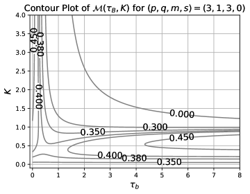
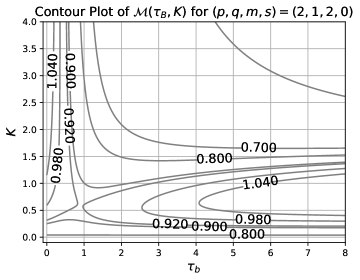
Figure 3: Level sets of $\mathcal{M}(\tau_{b},K)$ for Gierer-Meinhardt exponents $(p,q,m,s)=(3,1,3,0)$ (left) and $(p,q,m,s)=(2,1,2,0)$ (right). In both cases the level set value corresponds to a value of $\tau_{s}=M(\tau_{b},K)$. Note also the contours tending to a vertical asymptote, and the emergence of a horizontal asymptote as $\tau_{s}$ exceeds some threshold. Geometric parameters are $L=2\pi$ and $A=\pi$.

In the $(p,q,m,s)=(3,1,3,0)$ explicitly solvable case we find that $\text{Im}\mathcal{F}(i\lambda_{I}^{\star})=\tfrac{1}{3}\lambda_{I}^{\star}\text{Re}\mathcal{F}(i\lambda_{I}^{\star})$, so that by solving Re$\mathcal{A}_{0}(i\lambda_{I})=0$ for Re$\mathcal{F}(i\lambda_{I}^{\star})$, (3.12) becomes

$$\mathcal{M}(\tau_{b},K)=\frac{1+K}{3}-\frac{K\beta}{1+\beta}\left(\frac{\tfrac{\tau_{b}}{1+\beta}+\tfrac{1}{3}}{1+\bigl{(}\tfrac{\tau_{b}\lambda_{I}^{\star}}{1+\beta}\bigr{)}^{2}}\right)\,.$$

By substituting this expression into (3.11), we deduce the existence of two distinct threshold branches obtained by considering the limits $K\gg 1$ and $K\ll 1$. In this way, we derive

$$\tau_{s}-\mathcal{M}(\tau_{b},K)\sim\tau_{s}-\frac{1}{3}+\frac{1}{\beta_{0}}\biggl{(}\tau_{b}-\frac{1}{3}\biggr{)}+{\mathcal{O}}(K^{-1})\qquad\mbox{for}\quad K\gg 1\,,$$

$$\tau_{s}-\mathcal{M}(\tau_{b},K)\sim\tau_{s}-\frac{1}{3}-\frac{1}{3}K+{\mathcal{O}}(K^{2})\qquad\mbox{for}\qquad K\ll 1\,,$$

where $\beta_{0}\equiv L/A$. Notice that in ordering both of these asymptotic expansions we have used that $0<\lambda_{I}^{\star}\leq\lambda_{I}^{F}$, where the upper bound is independent of $K$. In the $K\gg 1$ regime we deduce that if $\tau_{b}=\tfrac{1}{3}-\beta_{0}\bigl{(}\tau_{s}-\tfrac{1}{3}\bigr{)}$, then $\text{Im}\mathcal{A}_{0}(i\lambda_{I}^{\star})=0$ forces $K\rightarrow\infty$, implying the existence of a threshold branch emerging from $K=\infty$ at these parameter values. Furthermore, since $\tau_{b}$ approaches $0$ when $\tau_{s}$ tends to $\tfrac{1}{3}\bigl{(}\tfrac{1}{\beta_{0}}+1\bigr{)}$, we deduce that this branch will disappear for sufficiently large values of $\tau_{s}$. In addition, in the $K\ll 1$ regime we find that a new branch given by $K\approx 3\tau_{s}-1$ emerges when $\tau_{s}>\tfrac{1}{3}$. The left panel of Figure 3 shows the numerically-computed contours of $\mathcal{M}(\tau_{b},K)$ for the explicitly solvable case $(p,q,m,s)=(3,1,3,0)$. The right panel of Figure 3 shows a qualitatively similar behavior that occurs for the prototypical Gierer-Meinhardt parameter set $(p,q,m,s)=(2,1,2,0)$.

The preceding analysis does not directly predict in which regions synchronous instabilities exist, as it only provides the boundaries of these regions. We now outline a winding-number argument, related to that used in [21], that provides a hybrid analytical-numerical algorithm for calculating the synchronous instability threshold $D_{v}=D_{v}^{\star}(K,\tau_{b},\tau_{s})$. Furthermore, as we show below, this algorithm indicates that synchronous instabilities exist whenever $M(\tau_{b},K)<\tau_{s}$.

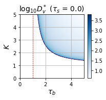
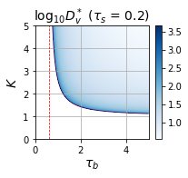
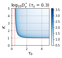
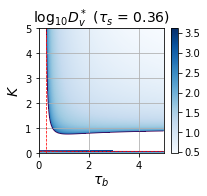
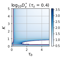
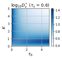
Figure 4: Colormap of the synchronous instability threshold $D_{v}^{\star}$ in the $K$ versus $\tau_{b}$ parameter plane for the well-mixed explicitly solvable case for various values of $\tau_{s}$ with $L=2\pi$ and $A=\pi$. The dashed vertical lines indicate the asymptotic predictions for the large $K$ threshold branch, while the dashed horizontal lines indicate the asymptotic predictions for the small $K$ threshold branch. The unshaded regions correspond to those parameter values for which synchronous instabilities are absent.

Synchronous instabilities are identified with the zeros to (2.33) having a positive real-part when $\chi(\lambda)$ in (2.33) is replaced by $\chi_{0}(\lambda)$. By using a winding number argument, the search for such zeros can be reduced from one over the entire right-half plane $\mbox{Re}(\lambda)>0$ to one along only the positive imaginary axis. Indeed, if we consider a counterclockwise contour composed of a segment of the imaginary axis, $-\rho\leq\text{Im}\lambda\leq\rho$, together with the semi-circle defined by $|\lambda|=\rho$ and $-\pi/2<\text{arg}\lambda<\pi/2$, then in the limit $\rho\rightarrow\infty$ the change in argument is

$$\Delta\text{arg}\,\mathcal{A}_{0}(\lambda)=2\pi(Z-1),$$ (3.13)

where $Z$ is the number of zeros of $\mathcal{A}_{0}$ with positive real-part. Here we have used that $\chi_{0}(\lambda)\neq 0$ when $\text{Re}(\lambda)\geq 0$, while $\mathcal{F}(\lambda)$ has exactly one simple (and real) pole in the right-half plane corresponding to the only positive eigenvalue of the self-adjoint local operator $\mathcal{L}_{0}$ (cf. [22]). We immediately note that $\mathcal{F}(\lambda)={\mathcal{O}}(\lambda^{-1})$ for $|\lambda|\gg 1$, $|\arg\lambda|<\pi/2$, whereas

$$\mathcal{C}_{0}(\lambda)\sim 2\mu_{0}(0)\sqrt{\tau_{s}D_{v}}\lambda^{1/2}\,,\qquad\mathcal{C}_{0}(\lambda)\sim\mu_{0}(0)\frac{N\sqrt{D_{v}\tau_{s}}}{\pi R}\lambda^{1/2}\,,\qquad\mbox{for}\quad|\lambda|\gg 1\,,\,\,\,|\arg\lambda|<\pi/2\,,$$

for the well-mixed limit and the disk cases, respectively. Therefore, in both cases we have $\mathcal{A}_{0}(\lambda)\sim{\mathcal{O}}(\lambda^{1/2})$ for $|\lambda|\gg 1$ with $|\arg\lambda|<\pi/2$, so that the change in argument over the large semi-circle is $\pi/2$. Furthermore, since the parameters in $\mathcal{A}_{0}(\lambda)$ are real-valued, the change in argument over the segment of the imaginary axis can be reduced to that over the positive imaginary axis. In this way, we deduce that

$$Z=\frac{5}{4}+\frac{1}{\pi}\Delta\text{arg}\mathcal{A}_{0}(i\lambda_{I})\bigr{|}_{\lambda_{I}\in(\infty,0]}.$$ (3.14)

We readily evaluate the limiting behaviour $\lim_{\lambda_{I}\rightarrow\infty}\text{arg}\,\mathcal{A}_{0}(i\lambda_{I})=\pi/4$. Moreover since $\chi_{0}(0)=1$ we evaluate $\mathcal{A}_{0}(0)=1-\tfrac{mq}{p-1}<0$ by the assumption (1.2) on the Gierer-Meinhardt exponents. Numerical evidence suggests that $\text{Re}\mathcal{A}_{0}(i\lambda_{I})$ increases monotonically with $\lambda_{I}$ and there should therefore be a unique $\lambda_{I}^{\star}$ for which $\text{Re}\mathcal{A}_{0}(i\lambda_{I}^{\star})=0$. We conclude that there are two positive values for the change in argument, and hence the number of zeros of ${\mathcal{A}}_{0}(\lambda)$ in $\mbox{Re}(\lambda)>0$ is dictated by the sign of $\text{Im}\mathcal{A}_{0}(i\lambda_{I}^{\star})$ as follows:

$$Z=2\quad\text{if}\quad\text{Im}\mathcal{A}_{0}(i\lambda_{I}^{\star})>0\,,\qquad\text{or}\qquad Z=0\quad\text{if}\quad\text{Im}\mathcal{A}_{0}(i\lambda_{I}^{\star})<0\,.$$ (3.15)

Note in particular that, in view of the expression (3.11) for $\text{Im}\mathcal{A}_{0}(i\lambda_{I})$, this criterion implies that synchronous instabilities will exist whenever $M(\tau_{b},K)<\tau_{s}$ in the previous analysis. Within this region, the criterion (3.15) suggests a simple numerical algorithm for iteratively computing the threshold value of $D_{v}=D_{v}^{\star}(K,\tau_{b},\tau_{s})$. Specifically, with all parameters fixed, we first solve $\text{Re}\mathcal{A}_{0}(i\lambda_{I})=0$ for $\lambda_{I}^{0}$. Then, we calculate $\text{Im}\mathcal{A}_{0}(i\lambda_{I}^{0})$ and increase (resp. decrease) $D_{v}$ if $\text{Im}\mathcal{A}_{0}(i\lambda_{I}^{0})<0$ (resp. $\text{Im}\mathcal{A}_{0}(i\lambda_{I}^{0})>0$ until $\text{Im}\mathcal{A}_{0}(i\lambda_{I}^{0})=0$. This procedure is repeated until $|\mathcal{A}_{0}(i\lambda_{I}^{0})|$ is sufficiently small.

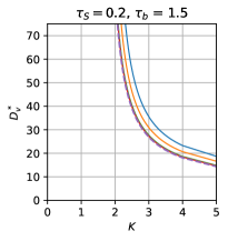
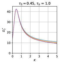
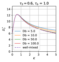
Figure 5: Synchronous instability threshold $D_{v}^{\star}$ versus $K$ for three pairs of $(\tau_{s},\tau_{b})$ for a one-spike steady-state ($N=1$) in the unit disk ($R=1$). The quality of the well-mixed approximation rapidly improves as $D_{b}$ is increased. The labels for $D_{b}$ in the right panel also apply to the left and middle panels.

Using the algorithm described above, the results in Figure 4 illustrate how the synchronous instability threshold $D_{v}^{\star}$ depends on parameters $\tau_{s}$, $\tau_{b}$, and $K$ for the explicitly solvable case in the well-mixed limit. From these figures we observe that coupling can have both a stabilizing and a destabilizing effect with respect to synchronous instabilities. Indeed, on the $K=0$ axis we see, as expected from the classical theory, that synchronous instabilities exist beyond some $\tau_{s}$ value. However, well before this threshold of $\tau_{s}$ is even reached it is possible for synchronous instabilities to exist when both $\tau_{b}$ and $K$ are sufficiently large. In contrast, we also see from the panels in Fig. 4 with $\tau_{s}=0.36$, $\tau_{s}=0.38$, and $\tau_{s}=0.4$ that when $\tau_{b}$ is sufficiently small, there are no synchronous instabilities when the coupling $K$ is large enough. Perhaps the most perplexing feature of this bulk-membrane interaction is the island of stability that arises around $\tau_{s}=0.4$ and appears to persist, propagating to larger values of $\tau_{b}$ as $\tau_{s}$ increases (only shown up to $\tau_{s}=0.6$). Finally in Figure 5 we demonstrate how the synchronous instability threshold behaves for finite bulk-diffusivity. A key observation from these plots is that that the instability threshold increases with decreasing value of $D_{b}$, which further supports our earlier monotonicity assumption.

3.4 Asynchronous Instabilities

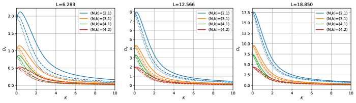
Figure 6: Asynchronous instability thresholds $D_{v}$ versus the coupling $K$ in the well-mixed limit for different values of $L$, different $(N,k)$ pairs, and for domain areas $A=3.142$ (solid), $1.571$ (dashed), and $0.785$ (dotted).

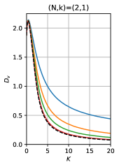
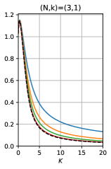
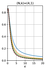
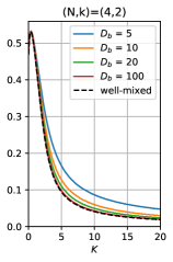
Figure 7: Asynchronous instability thresholds $D_{v}$ versus the coupling $K$ for the unit disk with Gierer-Meinhardt exponents $(3,1,3,0)$, and for different $D_{b}$. The dashed lines show the corresponding thresholds for the well-mixed limit. The legend in the right-most plot applies to each plot.

Since asynchronous instabilities emerge from a zero-eigenvalue crossing there are two significant simplifications. Firstly, the thresholds are determined by the nonlinear algebraic problem $\mathcal{A}_{k}(0)=0$, for each mode $k=1,\ldots,N-1$, as given by (2.33) in which $\chi(\lambda)$ is replaced by $\chi_{k}(\lambda)$ as defined in (3.5). Secondly, by setting $\lambda=0$, it follows that all $\tau_{s}$ and $\tau_{b}$ dependent terms in $\chi_{k}(\lambda)$ vanish. Therefore, asynchronous instability thresholds are independent of these two parameters. The resulting nonlinear algebraic equations are readily solved with an appropriate root finding algorithm (e.g. the brentq routine in the Python library SciPy). Furthermore, in the uncoupled case ($K=0$) the threshold can be determined explicitly (notice that when $K=0$ the well-mixed and disk cases coincide). Indeed, defining $z=\frac{L}{2N\sqrt{D_{v}}}$ and $y={\pi k/N}$, the algebraic problem $\mathcal{A}_{k}(0)=0$ becomes $\bigl{(}\tfrac{mq}{p-1}-1\bigr{)}\sinh^{2}(z)=\sin^{2}(y)$. From this relation it readily follows that the competition stability threshold for $K=0$ is

$$D_{v}=\biggl{[}\frac{2N}{L}\log\biggl{(}\sqrt{\tfrac{p-1}{mq-p+1}}\biggl{|}\sin\biggl{(}\frac{\pi k}{N}\biggr{)}\biggr{|}+\sqrt{\tfrac{p-1}{mq-p+1}\sin^{2}\biggl{(}\frac{\pi k}{N}\biggr{)}+1}\biggr{)}\biggr{]}^{-2}\,.$$ (3.16)

Figure 6 illustrates the dependence of the asynchronous threshold on the geometric parameters $L$ and $A$ for the well-mixed limit. In Figure 7 the effect of finite bulk diffusivity $D_{b}$ is explored for the unit disk. This figure also illustrates that while the asynchronous threshold tends to zero as $K\rightarrow\infty$ for sufficiently large values of $D_{b}$ the same is not true for small values of $D_{b}$. It is however worth remembering that for large $K$, where the competition threshold value of $D_{v}$ appears to approach zero in these figures, the result is not uniformly valid since the NLEP derivation required that $D_{v}\gg\varepsilon^{2}$.

3.5 Numerical Support of the Asymptotic Theory

In this subsection we verify some of the predictions of the steady-state and linear stability theory by performing full numerical PDE simulations of the coupled bulk-membrane system (1.1). In §3.5.1 we give an outline of the methods used for computing the full numerical solutions. In §3.5.2 and §3.5.3 we provide both quantitative and qualitative support for the instability thresholds predicted by the asymptotic theory.

3.5.1 Outline of Numerical Methods

The spatial discretization of (1.1) is much simpler for the well-mixed limit than for the case of the disk with a finite-bulk diffusivity. Indeed, in the well-mixed limit, the bulk inhibitor $V$ is spatially independent to leading order. By integrating the bulk PDE (1.1c), and using the divergence theorem, we obtain that $V$ satisfies the ODE

$$\tau_{b}V_{t}=-(\beta-1)V+\frac{\beta}{L}\int_{0}^{L}v\,d\sigma\,,$$ (3.17)

where $\beta\equiv{KL/A}$. For the well-mixed case it suffices to use a uniform grid in the arc-length coordinate for the spatial discretization of the membrane problem (1.1a) and (1.1b). Alternatively, the problem (1.1) for finite $D_{b}$ in the disk requires a full spatial discretization of the two-dimensional disk. To do so, we use a finite-element approach where the mesh is chosen in such a way that the boundary nodes are uniformly distributed. In this way, we can continue to apply a finite difference discretization for the membrane problem (1.1a) and (1.1b). For both the well-mixed case and the disk problem, the spatially discretized system leads to a large system of ODEs

$$\frac{dW}{dt}=\mathbb{A}W+F(W)\,.$$ (3.18)

Here the matrix $\mathbb{A}$ arises from the spatially discretized diffusion operator, while $F(W)$ denotes the reaction kinetics and the bulk-membrane coupling terms.

The choice of a time-stepping scheme for reaction diffusion systems is generally non-trivial. Since the operator $\mathbb{A}$ is stiff, it is best handled using an implicit time-stepping method. On the other hand, the kinetics $F(W)$ are typically non-linear so explicit time-stepping is favourable. Using a purely implicit or explicit time-stepping algorithm therefore leads to substantial computation time, either by requiring the use of a non-linear solver to handle the kinetics in the first case, or by requiring a prohibitively small time-step to handle the stiff linear operator in the second case. This difficulty can be circumvented by using so-called mixed methods, specifically the implicit-explicit methods described in [1]. We will use a second order semi-implicit backwards difference scheme (2-SBDF), which employs a second-order backwards difference to handle the diffusive term together with an explicit time-stepping strategy for the nonlinear term (cf. [18]). This time-stepping strategy is given by

$$(3\mathbb{I}-2\Delta t\mathbb{A})W^{n+1}=4W^{n}+4\Delta tF(W^{n})-W^{n-1}-2\Delta tF(W^{n-1})\,.$$ (3.19)

To initialize this second-order method we bootstrap with a first order semi-implicit backwards difference scheme (1-SBDF) as follows:

$$(\mathbb{I}-\Delta t\mathbb{A})W^{n+1}=W^{n}+\Delta tF(W^{n})\,.$$ (3.20)

We will use the numerical method outlined above in the two proceeding sections.

3.5.2 Quantitative Numerical Validation: Numerically Computed Synchronous Threshold

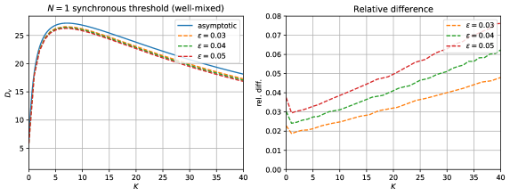
Figure 8: Comparison between numerical and asymptotic synchronous instability threshold for $N=1$ with $L=2\pi$, $A=\pi$, $\tau_{s}=0.6$, and $\tau_{b}=0.01$. Notice that, as expected, the agreement improves as $\varepsilon$ decreases.

We begin by describing a method for numerically calculating the synchronous instability threshold for a one (or more) spike pattern. Given an equilibrium solution $(u_{0},v_{0},V_{0})$, for sufficiently small times the numerical solution will evolve approximately as the linearization

$$u(\sigma,t)=u_{0}(\sigma)+e^{\lambda t}\phi(\sigma)\,,\qquad v(\sigma,t)=v_{0}(\sigma)+e^{\lambda t}\psi(\sigma)\,,\qquad V(\sigma,t)=V_{0}(\sigma)+e^{\lambda t}\eta(\sigma)\,.$$

For $\varepsilon>0$ fixed and sufficiently small the steady-state will be very close to that predicted by the asymptotic theory. By initializing the numerical solver with one of the steady-state solutions predicted by the asymptotic theory, and then tracking its time evolution, we will thus be able to approximate the value of $\text{Re}(\lambda)$. If we fix a location on the boundary $\sigma^{\star}$ (e.g. one of the spike locations) and let $t_{1}^{\star}<t_{2}^{\star}<...$ denote the sequence of times at which $u(\sigma^{\star},t)$ attains a local maximum or minimum in $t$, then the sequence $u_{j}^{\star}=u(\sigma^{\star},t_{j}^{\star})$ ($j=1,..,$) will approximate the envelope of $u(\sigma^{\star},t)$. If this sequence is diverging from its average then $\text{Re}\lambda\geq 0$, whereas if it is converging then $\text{Re}\lambda<0$. Furthermore, by writing

$$|u_{n}^{\star}-u_{0}(\sigma^{\star})|\approx e^{t_{n}\text{Re}(\lambda)}|\phi(\sigma^{\star})|\,,$$

we can solve for $\text{Re}(\lambda)$ by taking two values $t_{n}^{\star}>t_{m}^{\star}$ sufficiently far apart to get

$$\text{Re}(\lambda)\approx\frac{\log\bigl{|}u_{n}^{\star}-u_{0}(\sigma^{\star})\bigr{|}-\log\bigl{|}u_{m}^{\star}-u_{0}(\sigma^{\star})\bigr{|}}{t_{n}^{\star}-t_{m}^{\star}}\,.$$

This motivates a simple method for estimating the synchronous instability threshold numerically. Starting with some point in parameter space (chosen close to the threshold predicted by the asymptotic theory) we approximate $\text{Re}(\lambda)$ and then increase or decrease one of the parameters to drive $\text{Re}(\lambda)$ towards zero. Once $\text{Re}(\lambda)$ is sufficiently close to zero we designate the resulting point in parameter space as a numerically-computed synchronous instability threshold point.

In the well-mixed limit, we fix values of $K$ and vary $D_{v}$ using the numerical approach described above until $\text{Re}(\lambda)$ is sufficiently small. The results in Figure 8 compare the synchronous instability threshold for $N=1$ in the well-mixed limit as predicted by the asymptotic theory and by our full numerical approach for $\varepsilon=0.3,0.4,0.5$. We observe, as expected, that the asymptotic prediction improves with decreasing values of $\varepsilon$, but that the agreement is non-uniform in the coupling parameter $K$.

3.5.3 Qualitative Numerical Support: A Gallery of Numerical Simulations

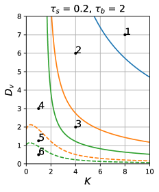
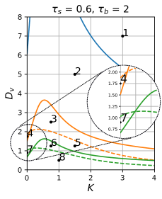
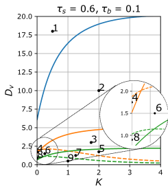
Figure 9: Synchronous (solid) and asynchronous (dashed) instability thresholds in the $D_{v}$ versus $K$ parameter plane in the well-mixed limit for $N=1$ (blue), $N=2$ (orange), and $N=3$ (green). At the top of each of the three panels a different pair $(\tau_{s},\tau_{b})$ is specified. See Table 1 for $D_{v}$ and $K$ values at the numbered points in each panel. Figures 10, 11, and 12 show the corresponding spike dynamics from full PDE simulations of (1.1) at the indicated points.

We conclude this section by first showcasing the dynamics of multiple spike patterns for several choices of the parameters $K$, $D_{v}$, $\tau_{s}$, and $\tau_{b}$ in the well-mixed limit. We will focus exclusively on the explicitly solvable Gierer-Meinhardt exponent set $(p,q,m,s)=(3,1,3,0)$ with $\varepsilon=0.05$ and the geometric parameters $L=2\pi$ and $A=\pi$. For the numerical computation we discretized the domain boundary with $1200$ uniformly distributed points ($\Delta\sigma\approx 0.00524$) and used trapezoidal integration for the bulk-inhibitor equation (3.17). Furthermore, we used 2-SBDF time-stepping initialized by 1-SBDF with a time-step size of $\Delta t=2.5(\Delta\sigma)^{2}\approx 6.854\times 10^{-4}$. In Figure 9 we plot the asymptotically predicted synchronous and asynchronous instability thresholds for three pairs of time-scale parameters: $(\tau_{s},\tau_{b})=(0.2,2),(0.6,2),(0.6,0.1)$. Each plot also contains several sample points whose $K$ and $D_{v}$ values are given in Table 1 below. The corresponding full PDE numerical simulations, tracking the heights of the spikes versus time, at these sample points are shown in Figures 10, 11, and 12. We observe that the initial instability onset in these figures is in agreement with that predicted by the linear stability theory. For example, when $\tau_{s}=0.6$ and $\tau_{b}=2$ an $N=3$ spike pattern at point six should be stable with respect to an $N=3$ synchronous instability but unstable with respect to the $N=3$ asynchronous instabilities. Indeed the initial instability onset depicted in the “point $6$, $N=3$” plot of Figure 11 showcases the non-oscillatory growth of two spikes and decay of one as expected. In addition the plots in Figures 10, 11, and 12 support two previously stated conjectures. Firstly, pure Hopf bifurcations for $N\geq 2$ should be supercritical (see “Point $4$, $N=2$”, “Point $7$, $N=3$” in Figure 11, and “Point $4$, $N=2$”, “Point $8$, $N=3$” in Figure 12). Secondly, we observe that asynchronous instabilities lead to the eventual annihilation of some spikes and the growth of others. As a result, our PDE simulations suggest that these instabilities are subcritical.

Point	$K$	$D_{v}$
1	8	7
2	4	6
3	4	2
4	1	3
5	1	1.25
6	1	0.5

(a)

Point	$K$	$D_{v}$
1	3	7
2	1.5	5
3	0.75	2.5
4	0	1.75
5	1.5	1.25
6	0.75	1.25
7	0	0.9
8	1	0.5

(b)

Point	$K$	$D_{v}$
1	0.5	18
2	2	10
3	1.75	3
4	0	1.75
5	2	1.75
6	0.25	1.5
7	1.25	1.25
8	0	0.9
9	1	0.9

(c)

Point	$K$	$D_{v}$
1	0.5	18
2	2	10
3	2	3.5
4	1	0.5
5	0.025	1.8

(d)

Table 1: $K$ and $D_{v}$ values at the sampled points in the three panels of Fig. 9: (a) Left panel: $(\tau_{s},\tau_{b})=(0.2,2)$, (b) Middle panel: $(\tau_{s},\tau_{b})=(0.6,2)$, and (c) Right panel: $(\tau_{s},\tau_{b})=(0.6,0.1)$. Table (d) shows the $K$ and $D_{v}$ values at the sampled points for the disk appearing in the left panel of Fig. 13.

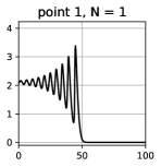
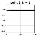
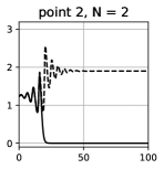
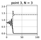
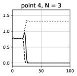
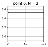
Figure 10: Numerically computed spike heights (vertical axis) versus time (horizontal axis) from full PDE simulations of (1.1) for $\tau_{s}=0.2$ and $\tau_{b}=2$ at the points indicated in the left panel of Figure 9. Distinct spike heights are distinguished by line types (solid, dashed, and dotted).

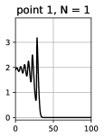
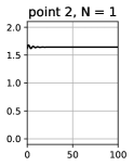
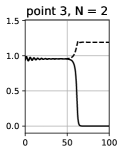
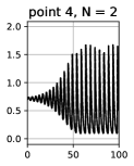
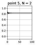
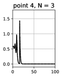
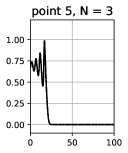
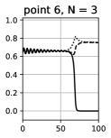
Figure 11: Numerically computed spike heights (vertical axis) versus time (horizontal axis) from full PDE simulations of (1.1) for $\tau_{s}=0.6$ and $\tau_{b}=2$ at the points indicated in the middle panel of Figure 9. Distinct spike heights are distinguished by line types (solid, dashed, and dotted).

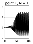
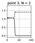
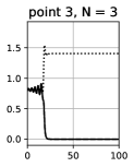
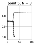
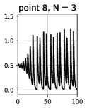
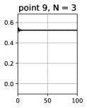
Figure 12: Numerically computed spike heights (vertical axis) versus time (horizontal axis) from full PDE simulations of (1.1) for $\tau_{s}=0.6$ and $\tau_{b}=0.1$ at the points indicated in the right panel of Figure 9. Distinct spike heights are distinguished by line types (solid, dashed, and dotted).

We now show that this agreement between predictions of our linear stability theory and results from full PDE simulations continues to hold for the case of a finite bulk diffusivity. To illustrate this agreement, we consider the unit disk with $D_{b}=10$ for $(\tau_{s},\tau_{b})=(0.6,0.1)$. For this parameter set, in the left panel of Figure 13 we show the asymptotically predicted synchronous and asynchronous instability thresholds in the $D_{v}$ versus $K$ parameter plane for $N=1$ and $N=2$. The faint grey dotted lines in this figure indicate the corresponding well-mixed thresholds. In the right panel of Figure 13 we plot the spike heights versus time, as computed numerically from (1.1), at the sample points indicated in the left panel. In each case, the numerically computed solution uses a $2\%$ perturbation away from the asymptotically computed $N$-spike equilibrium. As in the well-mixed case, the full numerical simulations confirm the predictions of the linear stability theory. Furthermore, Figures 1 and 2 depict both the bulk-inhibitor and the two membrane-bound species at certain times for an $N=2$ spike pattern at points $2$ and $5$ in the left panel of Figure 13, respectively. From this figure, we observe that the bulk-inhibitor field is largely constant except within a small near region near the spike locations.

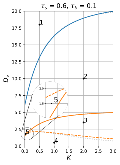
(a)

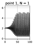
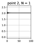
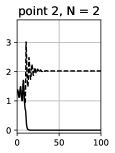
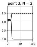
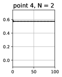
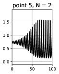
(b)

Figure 13: Left panel (a): Synchronous (solid) and asynchronous (dashed) instability thresholds in the $D_{v}$ versus $K$ parameter plane for the unit disk with $D_{b}=10$ and $(\tau_{s},\tau_{b})=(0.6,0.1)$. $N=1$ spike and $N=2$ spikes correspond to the (blue) and (orange) curves, respectively. The faint grey dotted lines are the corresponding well-mixed thresholds. Right panel (b): Numerically computed spike heights (vertical axis) versus time (horizontal axis) from full PDE simulations of (1.1) at the points indicated in the left panel for $N=1$ and $N=2$ spikes. For videos of the PDE simulations please see the supplementary materials.

4 The Effect of Boundary Perturbations on Asynchronous Instabilities

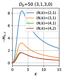
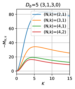
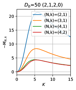
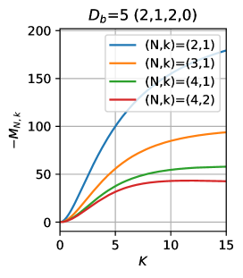
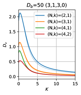
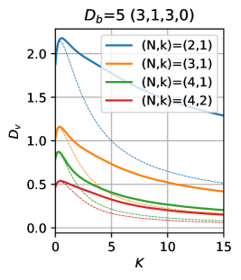
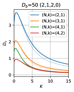
Figure 14: The effect of boundary perturbations on the asynchronous stability of symmetric $N$-spike patterns for the unit disk. The top row shows the multiplier $M_{N,k}$, defined in (4.7), as a function of $K$ while the bottom row shows the leading order correction to the asynchronous instability threshold, with the dashed line indicating the unperturbed threshold. Each column correspond to a choice of $D_{b}=50$ or $D_{b}=5$ with Gierer-Meinhardt exponents of $(p,q,m,s)=(3,1,3,0)$ or $(p,q,m,s)=(2,1,2,0)$. In the second row the boundary perturbation has parameters $\xi=1$ (indicating an outward bulge at the spike locations), and $\delta=0.01$.

The goal of this section is to calculate the leading order correction to the asynchronous instability thresholds for a perturbed disk. Specifically we consider the domain

$$\Omega_{\delta}\equiv\{(r,\theta)\,|\,0\leq r<R+\delta h(\theta)\,,\quad 0\leq\theta<2\pi\}\,,$$

where $h(\theta)$ is a smooth ${\mathcal{O}}(1)$ function with a Fourier series $h(\theta)=\sum_{n=-\infty}^{\infty}h_{n}e^{in\theta}$. Although our final results will be restricted to the specific form

$$h(\theta)=2R\xi\cos(N\theta)=R\xi e^{iN\theta}+R\xi e^{-iN\theta}\,,$$ (4.1)

where $\xi$ is a parameter, there is no additional difficulty in considering a general Fourier series in the analysis below. However, we remark that in using the general Fourier series given above we must impose appropriate symmetry conditions on $h(\theta)$ so that the symmetric $N$-spike pattern construction, and in particular the resulting NLEP (3.5), remain valid. Our main goal is to determine a two-term asymptotic expansion in powers of $\delta$ for each asynchronous instability threshold in the form

$$D_{v}\sim D_{vk0}^{\star}(D_{b},K,R)+D_{vk1}^{\star}(D_{b},K,R)\delta+{\mathcal{O}}(\delta^{2})\,,$$

such that a zero-eigenvalue crossing is maintained to at least second order, i.e. for which $\lambda={\mathcal{O}}(\delta^{2})$.

Recall that the only component of the asynchronous NLEP (3.5) that depends on the problem geometry is the NLEP multiplier $\chi_{k}(\lambda)$. To study the effect of boundary perturbations, it therefore suffices to calculate the leading order corrections to the corresponding membrane Green’s function satisfying (2.24). Furthermore, we note that since we are only interested in a first order expansion, whereas $\lambda={\mathcal{O}}(\delta^{2})$, there is no loss in validity assuming that $\lambda$ is an independent parameter that we ultimately set to zero. Upon expanding $D_{v}=D_{v0}\bigl{(}1+\tfrac{D_{v1}}{D_{v0}}\delta\bigr{)}$, a two-term expansion for the perturbed membrane Green’s function is given by (see Appendix B)

$$G_{\partial\Omega}^{\lambda}(\theta,\theta_{0})\sim G_{\partial\Omega 0}^{\lambda}(\theta,\theta_{0})+G_{\partial\Omega 1}^{\lambda}(\theta,\theta_{0})\delta+{\mathcal{O}}(\delta^{2}),$$

where $G_{\partial\Omega 0}^{\lambda}$ is the membrane Green’s function for the unperturbed disk calculated previously in (A.7) and the leading-order correction is

$$G_{\partial\Omega 1}^{\lambda}(\theta,\theta_{0})=-\tfrac{h(\theta_{0})}{R}G_{\partial\Omega 0}^{\lambda}(\theta,\theta_{0})+\tfrac{1}{2\pi R}\sum_{n=-\infty}^{\infty}\sum_{k=-\infty}^{\infty}\hat{g}_{n,k}^{\lambda}h_{n-k}g_{k}^{\lambda}g_{n}^{\lambda}e^{in\theta-ik\theta_{0}}-\tfrac{D_{v1}}{2\pi R^{3}}\sum_{n=-\infty}^{\infty}n^{2}(g_{n}^{\lambda})^{2}e^{in(\theta-\theta_{0})}\,.$$ (4.2)

In this expression the coefficients $\hat{g}_{n,k}^{\lambda}$ are given by

$$\hat{g}_{n,k}^{\lambda}=\tfrac{D_{v0}}{R^{3}}k(n+k)+K^{2}a_{k}^{\lambda}\bigl{(}\hat{a}_{n,k}^{\lambda}+P_{k}^{\prime}(R)\bigr{)}\,,$$ (4.3)

where $g_{k}^{\lambda}$, $a_{k}^{\lambda}$, and $\hat{a}_{n,k}^{\lambda}$ are defined in (3.9), (A.6), and (B.7), respectively.

Restricting our attention to perturbations of the form (4.1), and considering a symmetric $N$-spike pattern with spikes centered at $\theta_{j}=\tfrac{2\pi(j-1)}{N}$ for $j=1,...,N$, we deduce from (4.2) that

$$\begin{split}G_{\partial\Omega 1}^{\lambda}(\theta,\theta_{j})=-2\xi G_{\partial\Omega 0}^{\lambda}(\theta,\theta_{j})+\frac{\xi}{2\pi}\sum_{n=-\infty}^{\infty}\bigl{\{}\hat{g}_{n,n+N}^{\lambda}g_{0,n+N}^{\lambda}+\hat{g}_{n,n-N}^{\lambda}g_{0,n-N}^{\lambda}\}g_{0n}^{\lambda}e^{in(\theta-\theta_{j})}\\ -\tfrac{D_{v1}}{2\pi R^{3}}\sum_{n=-\infty}^{\infty}n^{2}(g_{0n}^{\lambda})^{2}e^{in(\theta-\theta_{j})}\,.\end{split}$$ (4.4)

Note that by symmetry the consistency and balance equations continue to hold for a symmetric $N$ spike pattern. Furthermore the perturbed Green’s matrix remains circulant, and therefore its eigenvalues can be read off as

$$\mu_{k}(\lambda)=\sum_{j=0}^{N-1}G_{\partial\Omega}^{\lambda}\bigl{(}\tfrac{2\pi}{N}j,0\bigr{)}e^{\frac{2\pi ijk}{N}}\sim\mu_{k0}(\lambda)+\delta\biggl{\{}-2\xi\mu_{k0}(\lambda)+\xi\mu_{k11}(\lambda)+D_{v1}\mu_{k12}(\lambda)\biggr{\}}\equiv\mu_{k0}(\lambda)+\delta\mu_{k1}(\lambda),$$

where

$$\mu_{k0}(\lambda) =\tfrac{N}{2\pi R}\sum_{n=-\infty}^{\infty}g_{nN-k}^{\lambda}\,,$$ (4.5a)

$$\mu_{k11}(\lambda) =\tfrac{N}{2\pi}\sum_{n=-\infty}^{\infty}\bigl{\{}\hat{g}_{nN-k,(n+1)N-k}^{\lambda}g_{(n+1)N-k}^{\lambda}+\hat{g}_{nN-k,(n-1)N-k}^{\lambda}g_{(n-1)N-k}^{\lambda}\bigr{\}}g_{nN-k}^{\lambda}\,,$$ (4.5b)

$$\mu_{k12}(\lambda) =-\tfrac{N}{2\pi R^{3}}\sum_{n=-\infty}^{\infty}(nN-k)^{2}(g_{nN-k}^{\lambda})^{2}\,.$$ (4.5c)

Finally, upon setting $\lambda=0$ in the zero-eigenvalue crossing condition $\mathcal{A}_{k}(0)=\left[\chi_{k}(0)\right]^{-1}-{mq/(p-1)}$ for the asynchronous modes $k=1,\ldots,N-1$ (see (2.35)), and noting $\chi_{k}(0)={\mu_{k}(0)/\mu_{0}(0)}$ from (3.5), we obtain that

$$\frac{\mu_{00}(0)+\delta\left[-2\xi\mu_{00}(0)+\xi\mu_{011}(0)+D_{v1}\mu_{012}(0)\right]}{\mu_{k0}(\lambda)+\delta\left[-2\xi\mu_{k0}(\lambda)+\xi\mu_{k11}(\lambda)+D_{v1}\mu_{k12}(\lambda)\right]}-\frac{mq}{p-1}=0\,,\qquad\mbox{for}\quad k=1,\ldots,N-1\,.$$ (4.6)

The leading-order problem is satisfied by the previously determined threshold $D_{v0}=D_{vk0}^{\star}(K,D_{b},R)$. On the other hand, by expanding (4.6) in powers of $\delta$, we obtain from equating ${\mathcal{O}}(\delta)$ terms in this expansion that

$$\xi\bigl{(}\mu_{011}(0)-\tfrac{mq}{p-1}\mu_{k11}(0)\bigr{)}+D_{v1}\bigl{(}\mu_{012}(0)-\tfrac{mq}{p-1}\mu_{k12}(0)\bigr{)}=0\,.$$

Upon solving for $D_{v1}=D_{vk1}^{\star}(K,D_{b},R)$ in this expression, we conclude that

$$D_{vk1}^{\star}=-M_{N,k}\xi\,,\qquad\mbox{where}\quad M_{N,k}\equiv\frac{\mu_{011}(0)-\tfrac{mq}{p-1}\mu_{k11}(0)}{\mu_{012}(0)-\tfrac{mq}{p-1}\mu_{k12}(0)}\,.$$ (4.7)

Therefore, the sign and magnitude of the multiplier $M_{N,k}$ determines how the asynchronous instability threshold changes when the boundary is perturbed by a single Fourier mode of the form (4.1).

Figure 14 illustrates the effect of boundary perturbations of the form (4.1) by plotting the multiplier $-M_{N,k}$ in the top row, and the leading order corrected asynchronous threshold $D_{v}\sim D_{vk0}^{\star}+D_{vk1}^{\star}\delta$ in the bottom row. Note that the (positive) maximums of $h(\theta)$ correspond with the quasi-equilibrium spike locations $\theta_{j}$ for each $j=1,...,N$. From (4.7) we therefore conclude that positive values of $-M_{N,k}$ indicate an increase in stability when spike locations bulge out ($\xi>0$), and a decrease in stability otherwise. The results of Figure 14 thus indicate that an outward bulge at the location of each spike in a symmetric $N$-spike pattern leads to an improvement in stability of the pattern with respect to asynchronous instabilities. In addition, the magnitude of $-M_{N,k}$ shows that this stabilizing effect is most pronounced at some finite value of $K$ corresponding to a maximum of $-M_{N,k}$. Furthermore, comparing the $D_{b}=50$ and $D_{b}=5$ plots we see that decreasing the bulk diffusivity further accentuates the effect of boundary perturbations as is clear from the relative magnitude of $-M_{N,k}$ in these two cases. These numerical observations lead us to propose the following numerically supported proposition.

Proposition 4.1

Consider a symmetric $N$-spike pattern for the Gierer-Meinhardt system (1.1) on the unit disk. Then a domain perturbation of the form (4.1), which creates an outward bulge at each spike location, will increase the asynchronous instability threshold of the symmetric $N$-spike pattern.

5 Discussion

We have introduced a coupled bulk-membrane PDE model in which a scalar linear 2-D bulk diffusion process is coupled through a linear Robin boundary condition to a two-component 1-D RD system with Gierer-Meinhardt (nonlinear) reaction kinetics defined on the domain boundary. For this coupled bulk-membrane PDE model, in the singularly perturbed limit of a long-range inhibition and short-range activation for the membrane-bound species, we have studied the existence and linear stability of localized steady-state multi-spike patterns defined on the membrane. Our primary goal was to study how the bulk diffusion process and the bulk-membrane coupling modifies the well-known linear stability properties of steady-state spike patterns for the 1-D Gierer-Meinhardt model in the absence of coupling.

By using a singular perturbation analysis on our coupled model (1.1) we first derived a nonlinear algebraic system (2.18) characterizing the locations and heights of steady-state multi-spike patterns on the membrane. Then we derived a new class of NLEPs (nonlocal eigenvalue problems) characterizing the linear stability on ${\mathcal{O}}(1)$ time-scales of these steady-state patterns. In this NLEP, the multiplier of the nonlocal term is determined in terms of the model parameters together with a new coupled nonlocal Green’s function problem. More specifically, a novel feature of our steady-state and linear stability analysis is the appearance of a nonlocal 1-D membrane Green’s function $G_{\partial\Omega}^{\lambda}(\sigma,\zeta)$ (see (2.24)), satisfying

$$D_{v}\partial_{\sigma}^{2}G_{\partial\Omega}^{\lambda}(\sigma,\zeta)-(1+K+\tau_{s}\lambda)G_{\partial\Omega}^{\lambda}(\sigma,\zeta)+K^{2}\int_{0}^{L}G_{\Omega}^{\lambda}(\sigma,\tilde{\sigma})G_{\partial\Omega}^{\lambda}(\tilde{\sigma},\zeta)\,d\tilde{\sigma}=-\delta(\sigma-\zeta)\,,\qquad 0<\sigma,\zeta<L\,,$$

which is coupled to a 2-D bulk Green’s function $G_{\Omega}^{\lambda}$ satisfying (see (2.21))

$$D_{b}\Delta G_{\Omega}^{\lambda}-(1+\tau_{b}\lambda)G_{\Omega}^{\lambda}=0\,,\quad\mbox{in}\,\,\,\,\Omega\,;\qquad D_{b}\partial_{n}G_{\Omega}^{\lambda}+KG_{\Omega}^{\lambda}=\delta_{\partial\Omega}(x-x_{0})\,,\quad\mbox{on}\,\,\,\,\partial\Omega\,.$$

Recall (1.1) for the description of all the model parameters including, the time constants $\tau_{s}$ and $\tau_{b}$, the diffusivities $D_{v}$ and $D_{b}$, and the coupling constant $K$.

To proceed with a more explicit linear stability theory we restricted our analysis to symmetric multi-spike patterns, which are characterized by equidistantly (in arc-length) separated spikes of equal height, for two analytically tractable cases. The first case is when $\Omega$ is a disk of radius $R$, while the second case is when the bulk is well mixed (i.e. $D_{b}\gg 1$). For these two specific cases, we obtained analytical expressions for the relevant Green’s function, and consequently the NLEP multipliers, in the form of infinite series for the disk and explicit formulae for the well-mixed limit. Parameter thresholds for two distinct forms of linear instabilities, corresponding to either synchronous or asynchronous perturbations of the heights of the steady-state spikes, were then computed from the NLEP. Our results indicate a non-monotonic dependence on the bulk-membrane coupling strength $K$ for both modes of instability, together with an intricate relationship between the time-scale and coupling parameters for the synchronous instabilities. Specifically, for the asynchronous instability modes the coupling has the effect of improving stability for smaller values of $K$ by raising the instability threshold for $D_{v}$, but reducing the range of stability for larger values of $K$. This effect is amplified in the synchronous case where for certain choices of $\tau_{s}$ a small region in the $K$ versus $\tau_{b}$ parameter space can be found for which no instabilities exist (see Figure 4). Finally, by using a Finite Element / Finite Difference mixed IMEX scheme, we confirmed our linear stability thresholds with full numerical PDE simulations.

We conclude the discussion by highlighting some open problems and directions for future research. Firstly, for our coupled model, additional work is required to calculate and study the linear stability of asymmetric spike patterns. Secondly, we have neglected the role of small $O(\varepsilon^{2})$ eigenvalues corresponding to weak drift instabilities, which can be studied either through a more detailed asymptotic analysis or by deriving and analyzing a corresponding slow spike-dynamics ODE system. Thirdly, the numerical evidence provided by our PDE simulations suggests that, when $N\geq 2$ in the absence of competition instabilities, the Hopf bifurcation is supercritical, and leads to the emergence of a small amplitude time-periodic solution near the bifurcation point. The numerical evidence also suggests that competition instabilities are subcritical, and result in the annihilation of one or more spikes in a multi-spike pattern. It would be worthwhile to analytically establish these conjectured branching behaviors from a weakly nonlinear analysis that is valid either near a Hopf bifurcation point or near a zero-eigenvalue crossing.

Finally, there are several directions for extending our model and applying a similar methodology. One direction would be to analyze similar problems in higher space dimensions, such as a 3-D linear bulk diffusion process coupled to a nonlinear RD system on a 2-D surface. A further direction would be to consider a two-component bulk diffusion process, with nonlinear bulk kinetics. For this more complicated model it would be interesting to study the interplay between 1-D membrane-bound and 2-D bulk-bound localized patterns. Additionally it would be instructive to asymptotically construct and analyze the localized patterns observed in the numerical study of Madzvamuse et. al. [12, 11] as well those of Rätz et. al. [15, 16, 17].

Appendix A Green’s Functions in the Well-Mixed Limit and for the Disk

In this appendix we collect all the relevant Green’s functions and indicate some of their key properties. We focus specifically on the uncoupled ($K=0$) Green’s function, the well-mixed Green’s function ($D_{b}\rightarrow\infty$), and the disk Green’s function ($\Omega=B_{R}(0)$). For the first two cases explicit formulae can be derived, while for the final case we must rely on a Fourier series expansion representation.

A.1 Uncoupled Membrane Green’s Function

When the bulk and membrane are uncoupled there is no direct dependence on the bulk Green’s function. Indeed the only relevant geometric dependent parameter becomes the perimeter of the domain $L=|\partial\Omega|$. Thus, $\Omega$ may be an arbitrary bounded and simply connected subset of $\mathbb{R}^{2}$. We define the uncoupled Green’s function $\Gamma^{\lambda}$ as the solution to

$$D_{v}\partial_{\sigma}^{2}\Gamma-\mu^{2}\Gamma=-\delta(\sigma-\zeta)\,,\qquad 0<\sigma<L\,,\qquad\Gamma\quad\mbox{is}\,\,L\text{-periodic}\,.$$ (A.1)

The solution to (A.1) is readily calculated as

$$\Gamma(\sigma,\zeta)=\frac{1}{2\sqrt{D_{v}}\mu}\coth\biggl{(}\frac{\mu L}{2\sqrt{D_{v}}}\biggr{)}\cosh\biggl{(}\frac{\mu}{\sqrt{D_{v}}}|\sigma-\zeta|\biggr{)}-\frac{1}{2\sqrt{D_{v}}\mu}\sinh\biggl{(}\frac{\mu}{\sqrt{D_{v}}}|\sigma-\zeta|\biggr{)}.$$ (A.2)

A.2 Bulk and Membrane Green’s functions in the Well-Mixed Limit

We now derive the leading order expression for the membrane Green’s function, defined by (2.24), when $D_{b}\rightarrow\infty$. To leading order $G_{\Omega}^{\lambda}$, defined by (2.21), is constant and from the divergence theorem we find

$$G_{\Omega}^{\lambda}(\sigma,\tilde{\sigma})\sim G_{\Omega 0}^{\lambda}=\frac{1}{KL+\mu_{b\lambda}^{2}A}=\frac{\beta/K}{\mu_{b\lambda}^{2}+\beta}\frac{1}{L}\,,\qquad\mbox{where}\quad\beta\equiv K\frac{L}{A}\,.$$ (A.3)

Here $L\equiv|\partial\Omega|$ and $A\equiv|\Omega|$. The leading order problem for the membrane Green’s function in (2.24) is then

$$D_{v}\partial_{\sigma}^{2}G_{\partial\Omega}^{\lambda}-\mu_{s\lambda}^{2}G_{\partial\Omega}^{\lambda}+K^{2}G_{\Omega 0}^{\lambda}\int_{0}^{L}G_{\partial\Omega}^{\lambda}(\tilde{\sigma};\zeta)\,d\tilde{\sigma}=-\delta(\sigma-\zeta)\,.$$ (A.4)

Upon integrating this equation and using the periodic boundary conditions we get

$$\int_{0}^{L}G_{\partial\Omega}^{\lambda}(\tilde{\sigma};\zeta)\,d\tilde{\sigma}=\frac{1}{\mu_{s\lambda}^{2}-K^{2}LG_{\Omega 0}^{\lambda}}=\left(\frac{1}{\mu_{s\lambda}^{2}(\mu_{b\lambda}^{2}+\beta)-K\beta}\right)\frac{1}{AG_{\Omega 0}^{\lambda}}\,,$$

where $G_{\Omega 0}^{\lambda}$ is defined in (A.3). Therefore, from (A.4), we find that $G_{\partial\Omega}^{\lambda}$ satisfies

$$D_{v}\partial_{\sigma}^{2}G_{\partial\Omega}^{\lambda}-\mu_{s\lambda}^{2}G_{\partial\Omega}^{\lambda}=-\delta(\sigma-\zeta)-\frac{K^{2}/A}{\mu_{s\lambda}^{2}(\mu_{b\lambda}^{2}+\beta)-K\beta}\,.$$

This problem is readily solved in terms of the uncoupled Green’s function of (A.2) by defining

$$\Gamma^{\lambda}(\sigma,\zeta):=\Gamma(\sigma,\zeta)\bigr{|}_{\mu=\mu_{s\lambda}}\,,$$

and then using the decomposition

$$G_{\partial\Omega}^{\lambda}(\sigma,\zeta)=\Gamma^{\lambda}(\sigma,\zeta)+\frac{K^{2}}{\mu_{s\lambda}^{2}A}\frac{1}{\mu_{s\lambda}^{2}(\mu_{b\lambda}^{2}+\beta)-K\beta}=\Gamma^{\lambda}(\sigma,\zeta)+\frac{\gamma_{\lambda}}{\mu_{s\lambda}^{2}}\,,\qquad\gamma_{\lambda}\equiv\frac{K^{2}/A}{\mu_{s\lambda}^{2}(\mu_{b\lambda}^{2}+\beta)-K\beta}\,.$$ (A.5)

A.3 Bulk and Membrane Green’s functions in the Disk

Here we consider the bulk Green’s function defined by (2.21). By using separation of variables (in polar coordinates), and applying the boundary condition in (2.21), we can write this Green’s function as a Fourier series

$$G_{\Omega}^{\lambda}(r,\sigma,\tilde{\sigma})=\frac{1}{2\pi R}\sum_{n=-\infty}^{\infty}a_{n}^{\lambda}P_{n}(r)e^{\tfrac{in}{R}(\sigma-\tilde{\sigma})}\,,\quad P_{n}(r)\equiv\frac{I_{|n|}(\omega_{b\lambda}r)}{I_{|n|}(\omega_{b\lambda}R)}\,,\quad a_{n}^{\lambda}\equiv\frac{1}{D_{b}P_{n}^{\prime}(R)+K}\,,\quad\omega_{b\lambda}\equiv\frac{\mu_{b\lambda}}{\sqrt{D_{b}}}\,.$$ (A.6)

We remark that the singularity lies on the boundary and for this reason the radial dependence is given only in terms of the modified Bessel functions of the first kind $I_{n}(z)$. Similarly, we can represent the membrane Green’s function in (2.24) for the disk in terms of the Fourier series

$$G_{\partial\Omega}^{\lambda}(\sigma,\sigma_{0})=\frac{1}{2\pi R}\sum_{n=-\infty}^{\infty}g_{n}^{\lambda}e^{\tfrac{in}{R}(\sigma-\sigma_{0})}\,,\qquad g_{n}^{\lambda}\equiv\frac{1}{D_{v}\tfrac{n^{2}}{R^{2}}+\mu_{s\lambda}^{2}-K^{2}a_{n}^{\lambda}}\,.$$ (A.7)

A.4 A Useful Summation Formula for the Disk Green’s Functions

We make note here of a useful summation formula for numerically evaluating the Green’s function eigenvalues for the disk. By integrating the function $(\zeta^{2}+z^{2})^{-1}\cot\bigl{(}\tfrac{\pi}{N}(\zeta-k)\bigr{)}$ over the contour enclosing $[-R,R]\times[-R,R]$, and then taking the limit $R\rightarrow\infty$, we obtain

$$S(z;N,k):=\sum_{n=-\infty}^{\infty}\frac{1}{(nN+k)^{2}+z^{2}}=\frac{\pi}{2Nz}\biggl{[}\coth\biggl{(}\frac{\pi}{N}(z+ik)\biggr{)}+\coth\biggl{(}\frac{\pi}{N}(z-ik)\biggr{)}\biggr{]}\,.$$ (A.8)

Appendix B Derivation of Membrane Green’s Function for the Perturbed Disk

In this appendix we provide the details for calculating the leading-order correction to the perturbed disk Green’s function given in (4.2). Recall that the bulk Green’s function solves

$$D_{b}\Delta G_{\Omega}^{\lambda}-\mu_{b\lambda}^{2}G_{\Omega}^{\lambda}=0,\quad\text{in}\quad\Omega_{\delta}\,,\qquad D_{b}\partial_{n}G_{\Omega}^{\lambda}+KG_{\Omega}^{\lambda}=\delta_{\partial\Omega_{\delta}}(x-\tilde{x}),\quad\text{on}\quad\partial\Omega_{\delta}\,.$$ (B.1)

On the boundary $r=R+\delta h(\theta)$ of the perturbed disk we calculate in terms of polar coordinates that

$$\hat{n}(\theta)=\bigl{[}1+\bigl{(}\tfrac{\delta h^{\prime}(\theta)}{R+\delta h(\theta)}\bigr{)}^{2}\bigr{]}^{-\frac{1}{2}}\bigl{(}\hat{e}_{r}-\tfrac{\delta h^{\prime}(\theta)}{R+\delta h(\theta)}\hat{e}_{\theta}\bigr{)}\,,\quad\nabla=\hat{e}_{r}\partial_{r}+\frac{1}{r}\hat{e}_{\theta}\partial_{\theta}\,,\quad\delta_{\partial\Omega_{\delta}}(x-\tilde{x})=\bigl{[}1+\bigl{(}\tfrac{\delta h^{\prime}(\theta)}{R+\delta h(\theta)}\bigr{)}^{2}\bigr{]}^{-\frac{1}{2}}\frac{\delta(\theta-\tilde{\theta})}{R+\delta h(\theta)}\,,$$

which yields the following asymptotic behaviour as $\delta\rightarrow 0$:

$$\hat{n}(\theta)\sim\hat{e}_{r}-\delta\frac{h^{\prime}(\theta)}{R}\hat{e}_{\theta}+{\mathcal{O}}(\delta^{2})\,,\qquad\delta_{\partial\Omega_{\delta}}(x-\tilde{x})\sim\frac{1}{R}\delta(\theta-\tilde{\theta})-\delta\frac{h(\theta)}{R^{2}}\delta(\theta-\tilde{\theta})+{\mathcal{O}}(\delta^{2})\,.$$

Next, for $\delta\ll 1$, we seek a solution of the form

$$G_{\Omega}^{\lambda}(r,\theta,\tilde{\theta}\sim G_{\Omega 0}^{\lambda}(r,\theta,\tilde{\theta})+G_{\Omega 1}^{\lambda}(r,\theta,\tilde{\theta})\delta+{\mathcal{O}}(\delta^{2})\,.$$

Upon substituting these expansions into (B.1), and collecting powers of $\delta$, we obtain the following zeroth-order and first-order problems:

$$D_{b}\Delta G_{\Omega 0}^{\lambda}-\mu_{b\lambda}^{2}G_{\Omega 0}^{\lambda}=0\,,\quad\text{in}\quad\Omega_{0}\,,\qquad\mathcal{B}_{0}G_{\Omega 0}^{\lambda}=\frac{\delta(\theta-\tilde{\theta})}{R}\,, \text{on}\quad\partial\Omega_{0}\,,$$ (B.2a)

$$D_{b}\Delta G_{\Omega 1}^{\lambda}-\mu_{b\lambda}^{2}G_{\Omega 1}^{\lambda}=0\,,\quad\text{in}\quad\Omega_{0}\,,\qquad\mathcal{B}_{0}G_{\Omega 1}^{\lambda}=-\frac{h(\theta)}{R}\frac{\delta(\theta-\tilde{\theta})}{R}-\mathcal{B}_{1}G_{\Omega 0}^{\lambda}, \text{on}\quad\partial\Omega_{0}\,,$$ (B.2b)

where the boundary operators $\mathcal{B}_{0}$ and $\mathcal{B}_{1}$ are defined by

$$\mathcal{B}_{0}\equiv D_{b}\partial_{r}+K\,\qquad\mathcal{B}_{1}\equiv D_{b}\biggl{(}h(\theta)\partial_{r}^{2}-\frac{h^{\prime}(\theta)}{R^{2}}\partial_{\theta}\biggr{)}+Kh(\theta)\partial_{r}.$$

The zeroth-order solution is the unperturbed disk bulk Green’s function given in (A.6). For the problem for the leading order correction, we use linearity to decompose its solution in the form

$$G_{\Omega 1}^{\lambda}(r,\theta,\tilde{\theta})=-\frac{h(\tilde{\theta})}{R}G_{\Omega 0}^{\lambda}(r,\theta,\tilde{\theta})+\tilde{G}_{\Omega 1}^{\lambda}(r,\theta,\tilde{\theta})\,,\qquad\tilde{G}_{\Omega 1}^{\lambda}(r,\theta,\tilde{\theta})=\frac{1}{2\pi R}\sum_{n=-\infty}^{\infty}\tilde{a}_{1n}^{\lambda}(\tilde{\theta})P_{n}(r)e^{in\theta}\,,$$ (B.3)

for some coefficients $\tilde{a}_{1n}^{\lambda}$ to be found. To determine an expression for these coefficients, we first multiply the boundary condition $\mathcal{B}_{0}\tilde{G}_{\Omega 1}^{\lambda}=-\mathcal{B}_{1}G_{\Omega 0}^{\lambda}$ by $e^{-in\theta}$, and then integrate from $0$ to $2\pi$. This gives

$$\frac{1}{R}\bigl{(}D_{b}P_{n}^{\prime}(R)+K)\tilde{a}_{1n}^{\lambda}(\tilde{\theta})=-\int_{0}^{2\pi}e^{-in\theta}\mathcal{B}_{1}G_{\Omega 0}^{\lambda}\,d\theta\,.$$ (B.4)

Then, by using the differential equation satisfied by $G_{\Omega 0}^{\lambda}$ we calculate the right-hand side of this expression as

$$\begin{split}\int_{0}^{2\pi}e^{-in\theta}\mathcal{B}_{1}G_{\Omega 0}^{\lambda}(R,\theta,\tilde{\theta})\,d\theta&=D_{b}\int_{0}^{2\pi}h(\theta)G_{\Omega 0rr}^{\lambda}(R,\theta,\tilde{\theta})e^{-in\theta}\,d\theta-\tfrac{D_{b}}{R^{2}}\int_{0}^{2\pi}h^{\prime}(\theta)G_{\Omega 0\theta}^{\lambda}(R,\theta,\tilde{\theta})e^{-in\theta}\,d\theta\\ &\qquad+K\int_{0}^{2\pi}h(\theta)G_{\Omega 0r}^{\lambda}(R,\theta,\tilde{\theta})e^{-in\theta}\,d\theta\,.\end{split}$$ (B.5)

Next, we assume that the boundary perturbation $h(\theta)$ is sufficiently smooth so that each of the following hold:

$$h(\theta)=\sum_{n=-\infty}^{\infty}h_{n}e^{in\theta}\,,\quad h^{\prime}(\theta)=i\sum_{n=-\infty}^{\infty}nh_{n}e^{in\theta}\,,\qquad h^{\prime\prime}(\theta)=-\sum_{n=-\infty}^{\infty}n^{2}h_{n}e^{in\theta}\,.$$ (B.6)

This allows us to calculate the individual terms on the right-hand side of (B.5) as

$$\int_{0}^{2\pi}h(\theta)G_{\Omega 0rr}^{\lambda}(R,\theta,\tilde{\theta})e^{-in\theta}d\theta=\frac{1}{R}\sum_{k=-\infty}^{\infty}P_{k}^{\prime\prime}(R)a_{k}^{\lambda}h_{n-k}e^{-ik\tilde{\theta}}\,,$$

$$\int_{0}^{2\pi}h^{\prime}(\theta)G_{\Omega 0\theta}^{\lambda}(R,\theta,\tilde{\theta})e^{-in\theta}d\theta=-\frac{1}{R}\sum_{k=-\infty}^{\infty}k(n-k)a_{k}^{\lambda}h_{n-k}e^{-ik\tilde{\theta}}\,,$$

$$\int_{0}^{2\pi}h(\theta)G_{\Omega 0r}^{\lambda}(R,\theta,\tilde{\theta})e^{-in\theta}d\theta=\frac{1}{R}\sum_{k=-\infty}^{\infty}P_{k}^{\prime}(R)a_{k}^{\lambda}h_{n-k}e^{-ik\tilde{\theta}}\,,$$

where $a_{k}^{\lambda}$ are the Fourier coefficients of the leading-order Green’s function, as defined in (A.6). By substituting these relations into (B.5), and then using (B.4), we determine the coefficients as

$$\tilde{a}_{1n}^{\lambda}(\tilde{\theta})=\sum_{k=-\infty}^{\infty}\hat{a}_{n,k}^{\lambda}a_{k}^{\lambda}h_{n-k}e^{-ik\tilde{\theta}}\,,\qquad\mbox{where}\qquad\hat{a}_{n,k}^{\lambda}\equiv-\frac{D_{b}P_{k}^{\prime\prime}(R)+KP_{k}^{\prime}(R)+\tfrac{D_{b}}{R^{2}}k(n-k)}{D_{b}P_{n}^{\prime}(R)+K}\,.$$ (B.7)

In (B.7), to calculate various derivatives of $P_{n}(R)$, as defined in (A.6), we make repeated use of the identity

$$I_{n}^{\prime}(z)=\frac{n}{z}I_{n}(z)+I_{n+1}(z)\,,$$

to readily derive that

$$P_{n}^{\prime}(R)=\frac{|n|}{R}+\omega_{b\lambda}\frac{I_{|n+1|}(\omega_{b\lambda}R)}{I_{|n|}(\omega_{b\lambda}R)}\,,\qquad P_{n}^{\prime\prime}(R)=\frac{|n|(|n|-1)}{R^{2}}+\frac{2|n|+1}{R}\omega_{b\lambda}\frac{I_{|n+1|}(\omega_{b\lambda}R)}{I_{|n|}(\omega_{b\lambda}R)}+\omega_{b\lambda}^{2}\frac{I_{|n+2|}(\omega_{b\lambda}R)}{I_{|n|}(\omega_{b\lambda}R)}\,.$$

This completes the derivation of the leading-order correction for the bulk Green’s function, defined in (B.3).

Next, we derive a two-term approximation for the membrane Green’s function problem on the perturbed disk. This Green’s function satisfies

$$D_{v}\partial_{\sigma}^{2}G_{\partial\Omega}^{\lambda}(\sigma,\sigma_{0})-\mu_{s\lambda}^{2}G_{\partial\Omega}^{\lambda}(\sigma,\sigma_{0})+K^{2}\int_{0}^{|\partial\Omega_{\delta}|}G_{\Omega}^{\lambda}(\sigma,\tilde{\sigma})G_{\partial\Omega}^{\lambda}(\tilde{\sigma},\sigma_{0})\,d\tilde{\sigma}=-\delta(\sigma-\sigma_{0}),\qquad 0\leq\sigma<|\partial\Omega_{\delta}|.$$ (B.8)

Repeated use of the chain rule to the arc-length formula

$$\sigma(\theta)=\int_{0}^{\theta}\bigl{(}R+\delta h(\vartheta)\bigr{)}\sqrt{1+\biggl{(}\frac{\delta h^{\prime}(\vartheta)}{R+\delta h(\vartheta)}\biggr{)}^{2}}\,d\vartheta\,,$$

gives

$$\partial_{\sigma}^{2}=\frac{1}{(R+\delta h(\theta))^{2}+(\delta h^{\prime}(\theta))^{2}}\partial_{\theta}^{2}-\delta h^{\prime}(\theta)\frac{R+\delta h(\theta)+\delta h^{\prime\prime}(\theta)}{[(R+\delta h(\theta))^{2}+(\delta h^{\prime}(\theta))^{2}]^{2}}\partial_{\theta}\,.$$

Multiplying the membrane equation through by $(R+\delta h(\theta))^{2}+(\delta h^{\prime}(\theta))^{2}$, writing $D_{v}=D_{v0}\bigl{(}1+\tfrac{D_{v1}}{D_{v0}}\delta\bigr{)}$, and then dividing through by $R^{2}\bigl{(}1+\tfrac{D_{v1}}{D_{v0}}\delta\bigr{)}$, we obtain the perturbed problem

$$\tfrac{D_{v0}}{R^{2}}\partial_{\theta}^{2}G_{\partial\Omega}^{\lambda}(\theta,\theta_{0})-\tfrac{D_{v0}}{R^{2}}\delta h^{\prime}(\theta)\tfrac{R+\delta[h(\theta)+h^{\prime\prime}(\theta)]}{(R+\delta h(\theta))^{2}+(\delta h^{\prime}(\theta))^{2}}\partial_{\theta}G_{\partial\Omega}^{\lambda}(\theta,\theta_{0})-\tfrac{\mu_{s\lambda}^{2}}{R^{2}}\tfrac{(R+\delta h(\theta))^{2}+(\delta h^{\prime}(\theta))^{2}}{1+\tfrac{D_{v1}}{D_{v0}}\delta}G_{\partial\Omega}^{\lambda}(\theta,\theta_{0})$$

$$+\tfrac{K^{2}}{R^{2}}\tfrac{(R+\delta h(\theta))^{2}+(\delta h^{\prime}(\theta))^{2}}{1+\tfrac{D_{v1}}{D_{v0}}\delta}\int_{0}^{2\pi}\bigl{(}G_{\Omega 0}^{\lambda}(R,\theta,\tilde{\theta})+\delta G_{\Omega 1}^{\lambda}(R,\theta,\tilde{\theta})+\delta h(\theta)G_{\Omega 0r}^{\lambda}(R,\theta,\tilde{\theta})\bigr{)}G_{\partial\Omega}^{\lambda}(\tilde{\theta},\theta_{0})\sqrt{(R+\delta h(\tilde{\theta}))^{2}+(\delta h^{\prime}(\tilde{\theta}))^{2}}\,d\tilde{\theta}$$

$$\qquad=-\tfrac{1}{R^{2}}\tfrac{\sqrt{(R+\delta h(\theta))^{2}+(\delta h^{\prime}(\theta))^{2}}}{1+\tfrac{D_{v1}}{D_{v0}}\delta}\delta(\theta-\theta_{0})\,.$$

To determine a two-term asymptotic solution to this problem, we expand the membrane Green’s function as

$$G_{\partial\Omega}^{\lambda}(\theta,\theta_{0})\sim G_{\partial\Omega 0}^{\lambda}(\theta,\theta_{0})+\delta G_{\partial\Omega 1}^{\lambda}(\theta,\theta_{0})+{\mathcal{O}}(\delta^{2})\,.$$

Upon substituting this expansion into the perturbed problem, and collecting powers of $\delta$, we obtain the following zeroth-order and first-order problems:

$$\mathcal{M}_{0}G_{\partial\Omega 0}^{\lambda}(\theta,\theta_{0})=-\tfrac{1}{R}\delta(\theta-\theta_{0})\,,\qquad\mathcal{M}_{0}G_{\partial\Omega 1}^{\lambda}(\theta,\theta_{0})=-\bigl{(}\tfrac{h(\theta)}{R}-\tfrac{D_{v1}}{D_{v0}}\bigr{)}\tfrac{1}{R}\delta(\theta-\theta_{0})-\mathcal{M}_{1}G_{\partial\Omega 0}^{\lambda}(\theta,\theta_{0})\,.$$ (B.9a)

Here we have defined the unperturbed membrane operator $$\mathcal{M}_{0}$$ by

$$\mathcal{M}_{0}\psi(\theta,\theta_{0})\equiv\tfrac{D_{v0}}{R^{2}}\partial_{\theta}^{2}\psi(\theta,\theta_{0})-\mu_{s\lambda}^{2}\psi(\theta,\theta_{0})+K^{2}\int_{0}^{2\pi}G_{\Omega 0}^{\lambda}(R,\theta,\tilde{\theta})\psi(\tilde{\theta},\theta_{0})R\,d\tilde{\theta}\,,$$ (B.9b)

and its leading-order correction $$\mathcal{M}_{1}$$ by

$$\begin{split}\mathcal{M}_{1}\psi(\theta,\theta_{0})\equiv&-\tfrac{D_{v0}}{R^{3}}h^{\prime}(\theta)\partial_{\theta}\psi(\theta,\theta_{0})-\mu_{s\lambda}^{2}\bigl{(}\tfrac{2h(\theta)}{R}-\tfrac{D_{v1}}{D_{v0}}\bigr{)}\psi(\theta,\theta_{0})\\ &+K^{2}\bigl{(}\tfrac{2h(\theta)}{R}-\tfrac{D_{v1}}{D_{v0}}\bigr{)}\int_{0}^{2\pi}G_{\Omega 0}^{\lambda}(R,\theta,\tilde{\theta})\psi(\tilde{\theta},\theta_{0})R\,d\tilde{\theta}+K^{2}\int_{0}^{2\pi}G_{\Omega 1}^{\lambda}(R,\theta,\tilde{\theta})\psi(\tilde{\theta},\theta_{0})R\,d\tilde{\theta}\\ &+K^{2}h(\theta)\int_{0}^{2\pi}G_{\Omega 0r}^{\lambda}(R,\theta,\tilde{\theta})\psi(\tilde{\theta},\theta_{0})R\,d\tilde{\theta}+K^{2}\int_{0}^{2\pi}G_{\Omega 0}^{\lambda}(R,\theta,\tilde{\theta})\psi(\tilde{\theta},\theta_{0})h(\tilde{\theta})\,d\tilde{\theta}\,.\end{split}$$ (B.9c)

The zeroth-order solution is that of the unperturbed disk and is given by (A.7). By linearity, we then seek the solution for the leading order correction in the form

$$G_{\partial\Omega 1}^{\lambda}(\theta,\theta_{0})=\bigl{(}\tfrac{h(\theta_{0})}{R}-\tfrac{D_{v1}}{D_{v0}}\bigr{)}G_{\partial\Omega 0}^{\lambda}(\theta,\theta_{0})+\tilde{G}_{\partial\Omega 1}^{\lambda}(\theta,\theta_{0})\,,$$ (B.10)

where $\tilde{G}_{\partial\Omega 1}^{\lambda}(\theta,\phi)$ now satisfies

$$\mathcal{M}_{0}\tilde{G}_{\partial\Omega 1}^{\lambda}(\theta,\theta_{0})=-\mathcal{M}_{1}G_{\partial\Omega 0}^{\lambda}(\theta,\theta_{0})\,.$$

We will represent the solution $\tilde{G}_{\partial\Omega 1}^{\lambda}$ in terms of a Fourier series as

$$\tilde{G}_{\partial\Omega 1}^{\lambda}(\theta,\theta_{0})=\frac{1}{2\pi R}\sum_{n=-\infty}^{\infty}\tilde{g}_{1n}^{\lambda}(\theta_{0})e^{in\theta}\,,$$ (B.11)

for some coefficients $\tilde{g}_{1n}^{\lambda}(\theta_{0})$ to be found. Similar to the calculation provided above for the perturbed bulk Green’s function, we obtain that

$$\tilde{g}_{1n}^{\lambda}(\theta_{0})=Rg_{0n}^{\lambda}\int_{0}^{2\pi}e^{-in\theta}\mathcal{M}_{1}G_{\partial\Omega 0}^{\lambda}(\theta,\theta_{0})\,d\theta\,.$$ (B.12)

By using (B.9c) we calculate the right-hand side of this expression as

$$\begin{split}\int_{0}^{2\pi}e^{-in\theta}\mathcal{M}_{1}G_{\partial\Omega 0}^{\lambda}(\theta,\theta_{0})d\theta&=-\tfrac{D_{v0}}{R^{3}}J_{1n}(\theta_{0})-\tfrac{2\mu_{s\lambda}^{2}}{R}J_{2n}(\theta_{0})+\tfrac{\mu_{s\lambda}^{2}D_{v1}}{D_{v0}}J_{3n}(\theta_{0})\\ &\qquad+2K^{2}J_{4n}(\theta_{0})-\tfrac{K^{2}RD_{v1}}{D_{v0}}J_{5n}(\theta_{0})+K^{2}RJ_{6n}(\theta_{0})+K^{2}RJ_{7n}(\theta_{0})\,,\end{split}$$ (B.13)

where the various integrals $J_{1n},\ldots,J_{7n}$ are defined by

$$J_{1n}(\theta_{0})=\int_{0}^{2\pi}h^{\prime}(\theta)G_{\partial\Omega 0\theta}^{\lambda}(\theta,\theta_{0})e^{-in\theta}d\theta\,,\qquad J_{2n}(\theta_{0})=\int_{0}^{2\pi}h(\theta)G_{\partial\Omega 0}(\theta,\theta_{0})e^{-in\theta}d\theta\,,$$

$$J_{3n}(\theta_{0})=\int_{0}^{2\pi}G_{\partial\Omega 0}^{\lambda}(\theta,\theta_{0})e^{-in\theta}d\theta\,,\qquad J_{4n}(\theta_{0})=\int_{0}^{2\pi}\int_{0}^{2\pi}h(\theta)G_{\Omega 0}^{\lambda}(R,\theta,\tilde{\theta})G_{\partial\Omega 0}^{\lambda}(\tilde{\theta},\theta_{0})e^{-in\theta}d\tilde{\theta}d\theta\,,$$

$$J_{5n}(\theta_{0})=\int_{0}^{2\pi}\int_{0}^{2\pi}G_{\Omega 0}^{\lambda}(R,\theta,\tilde{\theta})G_{\partial\Omega 0}^{\lambda}(\tilde{\theta},\theta_{0})e^{-in\theta}d\tilde{\theta}d\theta\,,\qquad J_{6n}(\theta_{0})=\int_{0}^{2\pi}\int_{0}^{2\pi}\tilde{G}_{\Omega 1}^{\lambda}(R,\theta,\tilde{\theta})G_{\partial\Omega 0}^{\lambda}(\tilde{\theta},\theta_{0})e^{-in\theta}d\tilde{\theta}d\theta\,,$$

$$J_{7n}(\theta_{0})=\int_{0}^{2\pi}\int_{0}^{2\pi}h(\theta)G_{\Omega 0r}^{\lambda}(R,\theta,\tilde{\theta})G_{\partial\Omega 0}^{\lambda}(\tilde{\theta},\theta_{0})e^{-in\theta}d\tilde{\theta}d\theta\,.$$

By using the Fourier series representations for the leading-order bulk and membrane Green’s functions given in (A.6) and (A.7), respectively, together with (B.6) for $h(\theta)$, we calculate explicitly that

$$J_{1n}(\theta_{0})=-\frac{1}{R}\sum_{k=-\infty}^{\infty}k(n-k)h_{n-k}g_{k}^{\lambda}e^{-ik\theta_{0}}\,,\quad J_{2n}(\theta_{0})=\frac{1}{R}\sum_{k=-\infty}^{\infty}h_{n-k}g_{k}^{\lambda}e^{-ik\theta_{0}}\,,\quad J_{3n}(\theta_{0})=\frac{1}{R}g_{n}^{\lambda}e^{-in\theta_{0}}\,,$$

$$J_{4n}(\theta_{0})=\frac{1}{R^{2}}\sum_{k=-\infty}^{\infty}h_{n-k}a_{k}^{\lambda}g_{k}^{\lambda}e^{-ik\theta_{0}}\,,\quad J_{5n}(\theta_{0})=\frac{1}{R^{2}}a_{n}^{\lambda}g_{n}^{\lambda}e^{-in\theta_{0}}\,,$$

$$J_{6n}(\theta_{0})=\frac{1}{R^{2}}\sum_{k=-\infty}^{\infty}h_{n-k}\hat{a}_{n,k}^{\lambda}a_{k}^{\lambda}g_{k}^{\lambda}e^{-ik\theta_{0}}\,,\quad J_{7n}(\theta_{0})=\frac{1}{R^{2}}\sum_{k=-\infty}^{\infty}h_{n-k}P_{k}^{\prime}(R)a_{k}^{\lambda}g_{k}^{\lambda}e^{-ik\theta_{0}}\,.$$

Upon substituting these expressions into (B.13), and then recalling (B.12), we conclude that

$$\tilde{g}_{1n}^{\lambda}(\theta_{0})= g_{n}^{\lambda}\sum_{k=-\infty}^{\infty}\bigl{\{}\tfrac{D_{v0}}{R^{3}}k(n-k)-\tfrac{2\mu_{s\lambda}^{2}}{R}+\tfrac{2K^{2}}{R}a_{k}^{\lambda}+K^{2}\hat{a}_{n,k}^{\lambda}a_{k}^{\lambda}+K^{2}P_{k}^{\prime}(R)a_{k}^{\lambda}\bigr{\}}h_{n-k}g_{k}^{\lambda}e^{-ik\theta_{0}}$$

$$\qquad+\tfrac{D_{v1}}{D_{v0}}g_{n}^{\lambda}\bigl{(}\mu_{s\lambda}^{2}-2\pi K^{2}Ra_{n}^{\lambda}\bigr{)}g_{n}^{\lambda}e^{-in\theta_{0}}\,,$$

where the coefficients $a_{k}^{\lambda}$ are defined in (A.6). We can use the definition of the coefficients $g_{n}^{\lambda}$, as given in (A.7), to write $\mu_{s\lambda}^{2}-K^{2}a_{n}^{\lambda}=\tfrac{1}{g_{n}^{\lambda}}-\tfrac{D_{v0}}{R^{2}}n^{2}$. In this way, we get

$$\tilde{g}_{1n}^{\lambda}(\theta_{0})=\sum_{k=-\infty}^{\infty}\hat{g}_{n,k}^{\lambda}h_{n-k}g_{k}^{\lambda}e^{-ik\theta_{0}}g_{n}^{\lambda}+\bigl{(}\tfrac{D_{v1}}{D_{v0}}-\tfrac{2h(\theta_{0})}{R}\bigr{)}g_{n}^{\lambda}e^{-in\theta_{0}}-\tfrac{D_{v1}}{R^{2}}n^{2}(g_{n}^{\lambda})^{2}e^{-in\theta_{0}}\,,$$

where

$$\hat{g}_{n,k}^{\lambda}=\tfrac{D_{v0}}{R^{3}}k(n+k)+K^{2}a_{k}^{\lambda}\bigl{(}\hat{a}_{n,k}^{\lambda}+P_{k}^{\prime}(R)\bigr{)}.$$

Finally, from (B.10) and (B.11), we conclude that the first order correction for the membrane Green’s function is

$$G_{\partial\Omega 1}^{\lambda}(\theta,\theta_{0})=-\tfrac{h(\theta_{0})}{R}G_{\partial\Omega 0}^{\lambda}(\theta,\theta_{0})+\tfrac{1}{2\pi R}\sum_{n=-\infty}^{\infty}\sum_{k=-\infty}^{\infty}\hat{g}_{n,k}^{\lambda}h_{n-k}g_{k}^{\lambda}g_{n}^{\lambda}e^{in\theta-ik\theta_{0}}-\tfrac{D_{v1}}{2\pi R^{3}}\sum_{n=-\infty}^{\infty}n^{2}(g_{n}^{\lambda})^{2}e^{in(\theta-\theta_{0})}\,.$$

References

- [1] U. M. Ascher, S. J. Ruuth, and B. T. R. Wetton. Implicit-explicit methods for time-dependent partial differential equations. SIAM J. Numer. Anal., 32(3):797–823, 1995.
- [2] D. Cusseddu, L. Edelstein-Keshet, J. A. Mackenzie, S. Portet, and A. Madzvamuse. A coupled bulk-surface model for cell polarisation. J. Theor. Bio., 2018.
- [3] A. Doelman, R. A. Gardner, and T. Kaper. Large stable pulse solutions in reaction-diffusion equations. Indiana U. Math. Journ., 50(1):443–507, 2001.
- [4] A. Doelman, R. A. Gardner, and T. Kaper. Stability of spatially periodic pulse patterns in a class of singularly perturbed reaction-diffusion equations. Indiana U. Math. Journ., 54(5):1219–1301, 2005.
- [5] C. M. Elliott, T. Ranner, and C. Venkataraman. Coupled bulk-surface free boundary problems arising from a mathematical model of receptor-ligand dynamics. SIAM J. Math. Anal., 49(1):360–397, 2017.
- [6] A. Gierer and H. Meinhardt. A theory of biological pattern formation. Kybernetik, 12(1):30–39, Dec 1972.
- [7] A. Gomez-Marin, J. Garcia-Ojalvo, and J. M. Sancho. Self-sustained spatiotemporal oscillations induced by membrane-bulk coupling. Phys. Rev. Lett., 98:168303, Apr 2007.
- [8] D. Iron, M. J. Ward, and J. Wei. The stability of spike solutions to the one-dimensional Gierer-Meinhardt model. Phys. D, 150(1-2):25–62, 2001.
- [9] H. Levine and W.-J. Rappel. Membrane-bound Turing patterns. Phys. Rev. E (3), 72(6):061912, 5, 2005.
- [10] C. B. Macdonald, B. Merriman, and S. J. Ruuth. Simple computation of reaction-diffusion processes on point clouds. Proc. Natl. Acad. Sci. USA, 110(23):9209–9214, 2013.
- [11] A. Madzvamuse and A. H. Chung. The bulk-surface finite element method for reaction diffusion systems on stationary volumes. Finite Elements in Analysis and Design, 108:9–21, 2016.
- [12] A. Madzvamuse, A. H. W. Chung, and C. Venkataraman. Stability analysis and simulations of coupled bulk-surface reaction-diffusion systems. Proc. A., 471(2175):20140546, 18, 2015.
- [13] Y. Nec and M. J. Ward. An explicitly solvable nonlocal eigenvalue problem and the stability of a spike for a class of reaction-diffusion system. Math. Mod. Nat. Phen., 8(2):55–87, 2013.
- [14] Y. Nishiura. Far-from Equilibrium dynamics: Translations of mathematical monographs, volume 209. AMS Publications, Providence, Rhode Island, 2002.
- [15] A. Rätz and M. Röger. Turing instabilities in a mathematical model for signaling networks. J. Math. Biol., 65(6-7):1215–1244, 2012.
- [16] A. Rätz and M. Röger. Erratum to: Turing instabilities in a mathematical model for signaling networks [mr2993944]. J. Math. Biol., 66(1-2):421–422, 2013.
- [17] A. Rätz and M. Röger. Symmetry breaking in a bulk-surface reaction-diffusion model for signalling networks. Nonlinearity, 27(8):1805–1827, 2014.
- [18] S. J. Ruuth. Implicit-explicit methods for reaction-diffusion problems in pattern formation. J. Math. Biol., 34(2):148–176, 1995.
- [19] A. M. Turing. The chemical basis of morphogenesis. Philos. Trans. Roy. Soc. London Ser. B, 237(641):37–72, 1952.
- [20] M. J. Ward and J. Wei. Hopf bifurcation and oscillatory instabilities of spike solutions for the one-dimensional Gierer-Meinhardt model. J. Nonlinear Science, 13(2):209–264, 2003.
- [21] M. J. Ward and J. Wei. Hopf bifurcation of spike solutions for the shadow Gierer-Meinhardt model. European J. Appl. Math., 14(6):677–711, 2003.
- [22] J. Wei. On single interior spike solutions of the Gierer-Meinhardt system: uniqueness and spectrum estimates. European J. Appl. Math., 10(4):353–378, 1999.
- [23] J. Wei and M. Winter. Mathematial aspects of pattern formation in biological systems, volume 189. Applied Mathematical Sciences Series, Springer, 2014.