Accurate Computation of Light Curves and the Rossiter–McLaughlin Effect in Multi-Body Eclipsing Systems

Abstract

We present here an efficient method for computing the visible flux for each body during a multi-body eclipsing event for all commonly used limb darkening laws. Our approach follows the idea put forth by Pál (2012) to apply Green’s Theorem on the limb darkening integral, thus transforming the two-dimensional flux integral over the visible disk into a one-dimensional integral over the visible boundary. We implement this idea through an iterative process which combines a fast method for describing the visible boundary of each body with a fast numerical integration scheme to compute the integrals. For the two-body case, our method compares well in speed with both that of Mandel & Agol (2002) and that of Giménez (2006a). The strength of the method is that it works for any number of spherical bodies, with a computational accuracy that is adjustable through the use of a tolerance parameter. Most significantly, the method offers two main advantages over previously used techniques: (i) it can employ a multitude of limb darkening laws, including all of the commonly used ones; (ii) it can compute the Rossiter-McLaughlin effect for rigid body rotation with an arbitrary orientation of the rotation axis, using any of these limb darkening laws. In addition, we can compute the Rossiter-McLaughlin effect for stars exhibiting differential rotation, using the quadratic limb darkening law. We provide the mathematical background for the method and explain in detail how to implement the technique with the help of several examples and codes which we make available.

2018 December 6

1 Introduction

The eminent astronomer Henry Norris Russell asserted “… there are ways of approach to unknown territory which lead surprisingly far, and repay their followers richly. There is probably no better example of this than eclipses of heavenly bodies” (Russell, 1948). Russell’s declaration of the “royal road” to stellar astrophysics and, by extension, nearly all branches of astronomy, has indeed been fulfilled by the study of eclipsing binary stars. Russell’s pioneering work, with Harlow Shapley, and later with Merrill, provided the means to travel down this road (see Russell 1912; Russell & Shapely 1912; Russell & Merrill 1952). But the Russell-Merrill method was a product of its time (decades before the advent of computers), and although the method was employed into the 1970s, its limitations were apparent in the 1950s, highlighted most notably by Zdeněk Kopal (e.g. see Kopal 1959, Kopal 1979). Kopal’s own approach was both more mathematically robust and faithful to the data (e.g. using an iterative least-squares approach to matching observations). However it would take until the late 1960s and 1970s before computational resources allowed the use of light curve synthesis and modeling techniques (e.g. Lucy 1968, and the famous code of Wilson & Devinney 1971). Since then, eclipse modeling codes have grown more and more sophisticated, incorporating additional astrophysics and data-fitting methods (for a concise review of the development of binary star research, see Southworth 2012 and references therein).

The discovery of exoplanets near the turn of the 21st century, and in particular transiting exoplanets, created a resurgence of development in eclipse-modeling tools. While assumptions of sphericity greatly simplify the problem, the extreme radius ratio of the bodies requires very high spatial resolution on the star, becoming very computationally expensive for methods that “tile” the bodies then numerically integrate the surface elements (“pixels”). In addition, the quality of transit data, especially Kepler observations, required very high-fidelity modeling. To overcome these challenges, analytic methods for computing transits were developed that were vastly faster than summing surface tiles. Most notably, the method presented in Mandel & Agol (2002) - hereafter MA2002 - has seen widespread use and been employed in a great many investigations. The method presents analytic solutions, one for the four-parameter “nonlinear” limb darkening law of Claret (2000), and another for the quadratic limb darkening law (Kopal, 1950). Eleven different configurations of planet-over-star are given and analytic expressions are provided for each case. The nonlinear limb darkening requires evaluations of hypergeometric functions while the quadratic law requires elliptic integrals (which are much faster to evaluate).

A comlimentary approach to computing transit light curves was presented by Giménez (2006a). Inspired by Kopal’s work, the method is based on the cross-correlation of two optical apertures. By casting the problem in the language of physical optics, the wealth of mathematics developed for that field could be employed. Specifically, the light loss during an eclipse is expressed as a Hankel (or Fourier-Bessel) transform which can be evaluated via the sum of Jacobi polynomials. The Giménez method is quite general, since the geometric factors are decoupled from the light curve factors. In this method the limb darkening is expressed as a power law expansion (Kopal, 1950). The method is valid for all manner of spherical two-body transits, occultations, and eclipses. The accuracy is set by the number of terms used in the summation of Jacobi polynomials. Giménez (2006b) also used the same approach to allow the fast computation of the Rossiter-McLaughlin (R-M) effect, which is a distortion in the radial velocity curve observed during a partial eclipse or transit – (Rossiter, 1924; McLaughlin, 1924).

Another method was developed by Kjurkchieva et al. (2013) that uses the fact that while the stellar intensity decreases from the center to the limb (according to some limb darkening law), the intensity is uniform along any given concentric circle (i.e. the intensity is function of radius only). The intersection of the planet’s boundary and these stellar concentric circles define arcs on the star that are “behind” the planet (i.e. interior to the planet’s disk). The sum of these arcs is the light of the star blocked by the planet. This allows the usual stellar surface area integral to be replaced with a single radial integral, computed numerically. A similar approach was taken by Kreidberg (2015) who devised a fast method that made full use of the azimuthal symmetry of the stellar intensity, greatly simplifying the problem. Any radially symmetric limb darkening law is supported, and despite solving the area integral numerically, Kreidberg shows that this method is an order of magnitude faster than the MA2002 analytic solution for the nonlinear limb darkening law. This is due to the poor convergence properties of the evaluation of the Appell hypergeometric function. We emphasize this important point – while a closed-form analytic solution might appear to always be preferred, ultimately all such functions are computed numerically, and in some cases the cost of evaluation of special functions exceeds that of a straightforward numerical integral.

With the advent of space-based transit surveys, particularly the Kepler Mission (Borucki 2016 and references therein), light curves with continuous duration and precision orders of magnitude better than ground-based observations became available. This enabled the detection of exotic eclipses, a result of systems with more than two eclipsing bodies. Such systems include triply-eclipsing systems, circumbinary planets, and overlapping transits in systems with several planets. The Kepler Eclipsing Binary Star catalog (Kirk et al. 2016; see also Orosz 2015) lists 14 cases of triply eclipsing systems with two particularly noteworthy examples: KOI-126 Carter et al. (2011), and KIC 2856960, Marsh et al. (2014). Circumbinary planets (e.g. Doyle et al. 2011) and systems with multiple transiting planets (e.g. KOI-94, Hirano et al. 2012) can exhibit complex syzygy transits. Obviously such eclipses/transits cannot be modeled by simply repeatedly applying the previous algorithms. A way to model these complex eclipses/transits was needed.

Spurred by necessity and fueled by ingenuity, the solution appeared remarkably quickly. Kipping (2011) extended the work of Mandel & Agol to be able to handle the case of a small moon of a transiting exoplanet. Soon after, Pál (2012) presented a general method for handling transits of an arbitrary number of bodies of any size. While still treating the stars as spheres (i.e. disks on the plane of the sky), the method differs from the Mandel & Agol and the Giménez/Kopal methods. In essence, by using Green’s theorem, the integral over the visible surface areas of the eclipsed star is replaced with line integrals over the bounding arcs created by the circular edges of the transiting bodies. The exact analytic expressions for the linear limb darkening law, using incomplete elliptic integrals, is given by Pál. The accompanying code provided can handle linear and quadratic limb darkening laws for an arbitrary number of bodies. More recently, Luger, Lustig-Yaeger, & Agol (2017) significantly extended the work of Kreidberg (2015) for any number of overlapping spheres (e.g. planet-planet eclipses). The semi-analytical method computes the eclipsed light as the sum of one-dimensional integrals of intensity-weighted elliptical segments on the occulted object. Notably, the method also allows for tabulated intensities in place of a parameterized limb-darkening law, irradiation of the planet by the host star (i.e. the planet’s “phase curve”), and a planet “hotspot” offset from the sub-stellar point to simulate advection of the incident stellar flux by winds – provided these effects are all radially symmetric.

In this paper, we present a modification and extension of the method pioneered by Pál (2012) for simultaneous eclipses involving spherical bodies. The method employs Green’s theorem, but does not rely on analytic closed-form expressions for the integrals, which can be difficult to derive. Rather, the integrals are evaluated numerically using highly accurate and efficient Gaussian quadrature. This provides flexibility that enables the method to easily handle any number of bodies of any size and all simple radial limb darkening prescriptions. An example of that flexibility is the natural ease with which the R-M effect can be computed for multiple overlapping eclipses, including differential rotation of the stars.

In §2 we give a brief description of the general mathematical approach, and in §3 we describe in detail the method of construction of the arcs that define the visible boundaries of the eclipsed star. The “1-forms” required for the eclipse and R-M effect integrals are developed and tabulated in §4, where differential rotation is also discussed. In §5 we compare our method with that of MA2002 and Giménez (2006a) for the simple two-body case, and with that of Pál (2012). In §6 we present a worked example to illustrate the method, using KOI-126. Several appendices are included in which we provide detail on the derivation of the exterior derivatives, as well as on the R-M effect with differential rotation. Working codes (in Matlab and FORTRAN) that can be used to compute the light curves and the R-M effect are made publicly available.

2 Method Overview

In the process of computing observables for eclipsing binary star systems one often encounters integrals of the form

$$\iint\displaylimits_{S_{\rm{vis}}}f(x,y,z)\cos(\gamma)dS$$ (1)

where $f=f(x,y,z)$ is a quantity such as intensity or rotational radial velocity, $\cos(\gamma)$ is the foreshortening ($\gamma$ is the angle between the surface normal and the direction to the observer), $dS$ is the surface area element, and the integral is evaluated over the visible surface $S$. Throughout this work, $(x,y,z)$ is a right hand co-ordinate system with $x$ and $y$ defining the plane of the sky (POS) and $z$ points towards the observer.

The goal of this paper is to present a fast, robust method for evaluating such integrals. If we project opaque spheres onto the POS, we have

$$\iint\displaylimits_{S_{\rm{vis}}}f(x,y,z)\cos(\gamma)dS=\iint\displaylimits_{\rm{D}_{\rm vis}}F(x,y)dA$$ (2)

where the surface area element is related to the disk area element by $dS=\sec(\gamma)dA$, and the integral is evaluated over the visible part of the disk, $D_{\rm vis}$.

In the language of the exterior calculus, the integrand $F(x,y)dA$ is a closed 2-form on the unit disk (scaled by the disk radius). By the Poincaré Lemma, there exists a 1-form $P(x,y)dx+Q(x,y)dy$, the exterior derivative of which is $F$:

$$d\wedge\big{[}P,Q\big{]}\stackrel{{\scriptstyle\text{def}}}{{=}}\frac{\partial Q}{\partial x}-\frac{\partial P}{\partial y}=F(x,y)$$ (3)

where d is the exterior derivative operator. Applying Green’s theorem we obtain:

$$\iint\displaylimits_{S_{\rm{vis}}}f(x,y,z)\cos(\gamma)dS=\iint\displaylimits_{D_{\rm{vis}}}F(x,y)dA=\oint\displaylimits_{\partial D_{\rm{vis}}}\big{[}P,Q\big{]}\bm{\cdot}\big{[}x^{\prime},y^{\prime}\big{]}d\varphi$$ (4)

where $x=x(\varphi)$ and $y=y(\varphi)$ is a right-hand oriented parametric curve describing the boundary of the visible region, $x^{\prime}$ and $y^{\prime}$ are the derivatives of $x$ and $y$ with respect to $\varphi$, and the integral is evaluated over the boundary of the visible disk ($\partial D_{\rm vis}$). Thus, the evaluation of the visible surface integral reduces to finding the description of the oriented parametric curve and to expressing the 1-form $Pdx+Qdy$ in terms of simple functions.

3 Development of the Bounding Curve: Construction from Arcs

During a multibody eclipse involving $\cal{N}$ bodies, we seek to compute the boundary of the visible portion of each body at a given time, $t_{0}$. It is assumed that the bodies are spherical and given in the front-to-back (i.e. nearest to furthest) order from the observer. It is also assumed that the light travel time effect (LTTE) has been accounted for in the positioning of the bodies’ centers at time $t_{0}$ (i.e. in the local frame, not the observer’s frame, in which we are observing the LTTE corrected two-dimensional view of the system on the POS). Because the projection of these spherical bodies on the POS are circles, our bounding curves will be composed of segments of circular arcs.

Consider a body, denoted by $N$, with radius $R_{N}$ and central POS co-ordinates $(\rm\xi_{N,x},\xi_{N,y})$. The visible portion of Body $N$ is bounded by arcs that are either on the circumference of Body $N$ itself or on the circumference of one or more additional bodies obstructing it. Consider one of these bodies, Body $M$, with radius $R_{M}$ and POS co-ordinates $(\rm\xi_{M,x},\xi_{M,y})$. Given these POS center positions and radii, the parametric equations of a bounding arc within the disk of body $N$ may be written in terms of co-ordinates with origin at the center of Body $N$, normalized by body $N$’s radius:

$$\begin{aligned} x&=\big{[}R_{M}\cos(\varphi)+\xi_{M,x}-\xi_{N,x}\big{]}/R_{N}\\ y&=\big{[}R_{M}\sin(\varphi)+\xi_{M,y}-\xi_{N,y}\big{]}/R_{N}\\ \end{aligned}$$ (5)

The starting and ending angles are measured from the positive x-axis in the POS co-ordinates of body $M$. In all cases the ending angle will be greater than the starting angle to preserve the right handed orientation of the arc. To do that, the domain of an arc is restricted to $[0,4\pi)$. To denote these various arcs that are described by Equation (5) we use the following notation:

$$Arc_{NM}=\bigg{[}\text{Back Body $N$, Arc Centered on Body $M$, Starting Angle, Total Angle, Ending Angle}\bigg{]}$$ (6)

$Arc_{NM}$ can be thought of as “an arc on the back body ($N$) centered on a front body ($M$) with the given starting and ending angles”. Note that $N\geq M$, and the Total Angle is used in some of the integration formulae and is otherwise added for computational convenience and debugging.

In general, the visible portion of Body $N$ is formed in part by the “shadows” cast by the bodies in front of it. Therefore, constructing the path that bounds this visible potion requires the use of the boundary of the shadowing bodies. We call the former boundary the “visible path” and the latter boundary the “shadow path”. We initialize the process with a front body which is entirely visible, hence the visible path is the boundary of the body itself. Likewise, since there are no other bodies, the shadow path is the boundary of the body itself. We use that shadow path to compute the visible path of the second body, which is behind the first one. The two bodies together form a shadow path, which is then used to compute the visible path on the next body. The process continues until the visible path of the body which is furthest from the observer is computed. In Appendix A, we provide a thorough discussion and worked examples on how to go about the process of arc construction.

4 Limb Darkening and Rossiter-McLaughlin effect 1-forms

After developing the right hand oriented parametric curve describing the boundary of the visible region in §3, we now turn to expressing the 1-form $Pdx+Qdy$ in terms of simple functions in the cases of intensity (limb darkening) and radial velocity (the R-M effect). This will complete the development of the line integral over the visible boundary (Equation 4). Note that in cases where we have data in different bandpasses, we do not need to redo the generation of the bounding arcs, but rather use those arcs with the appropriate limb darkening to compute the intensity in each bandpass.

4.1 Limb Darkening

First consider these various parametrized limb darkening laws:

$$I(\mu)/I_{0}=1-c_{1}(1-\mu)$$ Linear (7)

$$I(\mu)/I_{0}=1-c_{1}(1-\mu)-c_{2}(1-\mu)^{2}$$ Quadratic (8)

$$I(\mu)/I_{0}=1-a(1-\mu)-b(1-\sqrt{\mu})$$ Square Root (9)

$$I(\mu)/I_{0}=1-\sum_{j=1}^{4}c_{j}(1-\mu^{\frac{j}{2}})$$ Claret (4 parameter nonlinear) (10)

$$I(\mu)/I_{0}=1-l_{1}(1-\mu)-l_{2}\mu\log(\mu)$$ Logarithmic (11)

Note the following: (i) $I_{0}$ is the intensity at the center of the disk. (ii) $r^{2}=x^{2}+y^{2}\text{~{}~{}and~{}~{}}\mu=\sqrt{1-r^{2}}$. (iii) When modeling the data, Kipping (2013) recommends re-parametrization of the limb darkening laws that allow uniform sampling of the physical parameter space. For example, the re-parametrized Quadratic Law has coefficients $q_{1}=(c_{1}+c_{2})^{2}$ and $q_{2}=0.5c_{1}(c_{1}+c_{2})^{-1}$. (iv) Kipping’s log term differs from the one given here, in Equation 11 (see Espinoza & Jordán, 2016) (v) The Exponential Law is not physical, so it is omitted (see Espinoza & Jordán, 2016). (vi) Kipping (2016) proposed a 3-parameter limb darkening law that is a subset of the Claret 4-parameter law (the $c_{1}$ term is set to zero). (vii) Finally, it is understood that the limb darkening coefficients are wavelength or bandpass dependent. (viii) Equations B6 explicitly give the 1-forms $[P,Q]$ for any limb darkening given by: $I(\mu)/I_{0}=f(r^{2})=f(1-\mu^{2})$ (where $f$ is a continuous function on the disk $D$), and for the R-M effect based on that limb darkening. The specific form of the integral $G$ (Equation B5) will determine if $[P,Q]$ can be expressed in closed form, by a special function, or will require numerical evaluation.

As can be seen in Equations 7-11, all of the laws are a linear combination of a few common terms, namely, $\bm{1},~{}\mu^{\frac{1}{2}},~{}\mu,~{}\mu^{\frac{3}{2}},\mu^{2}$ and $\mu\log(\mu)$, where $\bm{1}$ is the identically one function. If we form a vector $\bm{C}$ of the coefficients and a vector $\bm{\Psi}$ of the simple functional expressions, each limb darkening law may be written as a dot product of $\bm{C}$ and $\bm{\Psi}$.

$$I(\mu)/I_{0}=\bm{C}\bm{\cdot}\bm{\Psi}$$ (12)

Our goal is to separate the integration over the boundary of the visible region from the application of the specific limb darkening coefficients. This will allow the computation of intensity for varying bands without redoing the boundary integration. For example, expanding the terms of the Quadratic law gives the equation of the linear combination as:

$$\begin{aligned} &I(\mu)/I_{0}=\big{[}1-(c_{1}+c_{2})\big{]}\bm{1}+(c_{1}+2c_{2})\mu-c_{2}\mu^{2}\\ \Longrightarrow~{}~{}~{}&\bm{C}=\big{[}\big{(}1-(c_{1}+c_{2})\big{)},(c_{1}+2c_{2}),-c_{2}\big{]}\text{~{}~{}and~{}~{}}\bm{\Psi}=\big{[}\bm{1},\mu,\mu^{2}\big{]}\end{aligned}$$

The dot product forms of Equations 7-11 are then given by:

$$\bm{C}=\big{[}(1-c_{1}),c_{1}\big{]}\text{~{}~{}and~{}~{}}\bm{\Psi}=\big{[}\bm{1},\mu\big{]}$$ Linear (13)

$$\bm{C}=\big{[}\big{(}1-(c_{1}+c_{2})\big{)},(c_{1}+2c_{2}),-c_{2}\big{]}\text{~{}~{}and~{}~{}}\bm{\Psi}=\big{[}\bm{1},\mu,\mu^{2}\big{]}$$ Quadratic (14)

$$\bm{C}=\big{[}\big{(}1-(a+b)\big{)},b,a\big{]}\text{~{}~{}and~{}~{}}\bm{\Psi}=[\bm{1},\mu^{\frac{1}{2}},\mu\big{]}$$ Square Root (15)

$$\bm{C}=\big{[}\big{(}1-(c_{1}+c_{2}+c_{3}+c_{4})\big{)},c_{1},c_{2},c_{3},c_{4}\big{]}\text{~{}~{}and~{}~{}}\bm{\Psi}=\big{[}\bm{1},\mu^{\frac{1}{2}},\mu,\mu^{\frac{3}{2}},\mu^{2}\big{]}$$ Claret (4 parameter nonlinear) (16)

$$\bm{C}=\big{[}(1-l_{1}),l_{1},-l_{2}\big{]}\text{~{}~{}and~{}~{}}\bm{\Psi}=\big{[}\bm{1},\mu,\mu\log(\mu)\big{]}$$ Logarithmic (17)

Table 1 provides the 1-forms $\big{[}P,Q\big{]}$ which are the exterior anti-derivatives of the $\Psi$ vector component functions. See Appendix B for the derivations.

Using this form of the limb darkening laws, we now update Equation (4):

$$I_{\rm vis}=\iint\displaylimits_{D_{\rm vis}}\big{(}\bm{C}\bm{\cdot}\bm{\Psi}\big{)}dA$$ (18)

The fractional flux can be defined as the quotient

$${\cal F}_{\rm vis}=I_{\rm vis}/I_{\rm total}$$ (19)

The computation of the fractional flux requires two evaluations of the $I_{\rm vis}$ integral, so we seek a computational form of this integral. By linearity of integration we obtain:

$$\begin{aligned} I_{\rm vis}=\bm{C}\bm{\cdot}\bigg{[}\iint\displaylimits_{D_{\rm vis}}\Psi_{1}dA,\,\,\bm{\ldots}\,\,,\iint\displaylimits_{D_{\rm vis}}\Psi_{n}dA\bigg{]}\end{aligned}$$ (20)

and by Green’s Theorem, we obtain the following form of $I_{\rm vis}$:

$$\begin{aligned} I_{\rm vis}=\bm{C}\bm{\cdot}\bigg{[}\oint\displaylimits_{\partial D_{\rm vis}}\big{[}P_{1},Q_{1}\big{]}\bm{\cdot}\big{[}x^{\prime},y^{\prime}]d\varphi,\,\,\bm{\ldots}\,\,,\oint\displaylimits_{\partial D_{\rm vis}}\big{[}P_{n},Q_{n}\big{]}\bm{\cdot}\big{[}x^{\prime},y^{\prime}]d\varphi\bigg{]}\end{aligned}$$ (21)

From $\S\ref{sec:boundingcurve}$, the boundary curve of the visible portion of star $N$ from the observer is a set of circular arcs given by the $VisiblePath(BodyN)$ stack, where each arc is represented in the form of Equation (6):

$$Arc_{NM}=\big{[}N,M,\varphi_{0},\Delta\varphi,\varphi_{1}\big{]}$$ (22)

In terms of co-ordinates with origin the center of body $N$ scaled by body $N$’s radius $R_{N}$, we have the following parametric description of this arc within the disk of body $N$:

$$\begin{aligned} x&=\big{[}R_{M}\cos(\varphi)+\xi_{M,x}-\xi_{N,x}\big{]}/R_{N}\\ y&=\big{[}R_{M}\sin(\varphi)+\xi_{M,y}-\xi_{N,y}\big{]}/R_{N}\\ \end{aligned}$$

where $R_{N}$ is the radius of Body N, $R_{M}$ is the radius of Body $M$ (with its center the point in the POS having co-ordinates $\xi$), and $\varphi_{0}\leq\varphi\leq\varphi_{1}$, with derivatives,

$$\begin{aligned} x^{\prime}&=\frac{-R_{M}}{R_{N}}\sin(\varphi)~{}~{}~{}~{}~{}~{}~{}y^{\prime}&=\frac{R_{M}}{R_{N}}\cos(\varphi)\end{aligned}$$ (23)

In addition, $x$ and $y$ simplify when $M=N$:

$$x=\cos\varphi~{},~{}~{}y=\sin\varphi$$ (24)

Thus,

$$\oint\displaylimits_{\partial D_{\rm{vis}}}\big{[}P_{j},Q_{j}\big{]}\bm{\cdot}\big{[}x^{\prime},y^{\prime}\big{]}d\varphi=\sum_{i=1}^{\rm{\#~{}of~{}Arcs}}(\pm 1)\int\displaylimits_{\varphi_{j_{0}}}^{\varphi_{j_{1}}}\big{[}P_{j},Q_{j}\big{]}\bm{\cdot}\big{[}x^{\prime}_{i},y^{\prime}_{i}\big{]}d\varphi$$ (25)

where $\pm 1$ is the orientation. The visible region is outside of all bodies $M<N$, thus the orientation is $-1$. When $M=N$, the visible region lies in body $N$, thus the orientation is $+1$. In the case $N=M$, implying $r=1$ and $\mu=0$, the 1-forms $\big{[}P_{j},Q_{j}\big{]}$ greatly simplify, with the integrand $\big{[}P_{j},Q_{j}\big{]}\cdotp\big{[}x^{\prime},y^{\prime}\big{]}$ now easily integrated ($P$ and $Q$ are given in Table 1, are derived in Appendix B and given in closed form in Appendix E).

4.2 The Rossiter McLaughlin Effect

Now consider the R-M effect, which is a perterbation of the eclipsed star’s apparent radial velocity due to obscuring a portion of the star’s rotationally radial velocity field during an eclipse event. Giménez (2006b) developed a computational method based on Kopal (1979). He begins with the following equation (Equation 1, Giménez 2006b):

$$\delta RV=\frac{{\iint}\displaylimits_{S_{\rm{vis}}}vI\cos(\gamma)dS}{{\iint}\displaylimits_{S_{\rm{vis}}}I\cos(\gamma)~{}dS}$$ (26)

where $\delta RV$ is the radial velocity RV perturbation, $v$ is the rotationally induced radial velocity of the star, $I=I(\mu)$ is any limb darkening law in its dot product form (Equations 13-17), and $\gamma$ and $dS$ are as before. Then, following Equation (4) for both the numerator (rotational radial velocity) and the denominator (intensity), we get

$$\delta RV=\frac{{\iint}\displaylimits_{D_{\rm{vis}}}v(x,y)IdA}{{\iint}\displaylimits_{D_{\rm{vis}}}IdA}=\frac{{\oint}\displaylimits_{\partial D_{\rm{vis}}}\big{[}P_{\rm RM},Q_{\rm RM}\big{]}\bm{\cdot}\big{[}x^{\prime},y^{\prime}\big{]}d\varphi}{{\oint}\displaylimits_{\partial D_{\rm{vis}}}\big{[}P_{\rm FF},Q_{\rm FF}\big{]}\bm{\cdot}\big{[}x^{\prime},y^{\prime}\big{]}d\varphi}$$ (27)

where we use the abbreviation $FF$ to denote flux fraction. Note that the denominator is the visible flux.

Define the rotation axis of the star in the dynamic co-ordinate system $(x,y,z)$, with the observer on the positive $z$ axis, as defined by Equation (1). Note that this differs from the system defined first by Hosokawa (1953) and then used again by Giménez (2006a). Since their emphasis was on simple binary systems and planetary transits, their $y$ axis was just the projection of the orbital pole on the POS. In this paper, we do not assume a simple 2 body system but rather a multi-body system.

$$\begin{aligned} \Theta_{\rm{rot}}&\stackrel{{\scriptstyle\text{def}}}{{=}}\text{angle in the $(x,y)$ plane from the y-axis}\\ \Phi_{\rm{rot}}&\stackrel{{\scriptstyle\text{def}}}{{=}}\text{angle from the $z$ axis (co-latitude)}\end{aligned}$$ (28)

If the axis of rotation of the star is the $z$-axis, then the righthand surface velocity field on the unit sphere is given by

$$\vec{v}(x,y,z)=\omega(-y,x,0)$$ (29)

where $\omega$ is the angular velocity in radians per day. Note that $\|(-y,x,0)\|$ is the distance to the axis of rotation (the $z$ axis).

Using Rotation Transformations (orthonormal matrices with determinant equals to $1$) move the $z$ axis to the rotation axis described by $\big{(}\Theta_{\rm{rot}},\Phi_{\rm{rot}}\big{)}$. Since the transformations are length and orientation preserving, the transformation of the velocity field is also preserved as the velocity field generated by a righthand rotation about the axis $\big{(}\Theta_{\rm{rot}},\Phi_{\rm{rot}}\big{)}$. The radial velocity function is simply the $z$-component of this velocity field. Namely,

$$v(x,y)=\omega\big{[}\sin(\Phi_{\rm rot})\cos(\Theta_{\rm rot})x+\sin(\Phi_{\rm rot})\sin(\Theta_{\rm rot})y\big{]}$$ (30)

for $(x,y)$ any point on the POS disk normalized to the unit disk. Note that the observed rotational velocity is $v_{\rm rot}\sin i=R_{\ast}\omega\sin(\Phi_{\rm{rot}})$, with $R_{*}$ the stellar radius.

Define

$$\begin{aligned} &A\stackrel{{\scriptstyle\text{def}}}{{=}}\sin(\Phi_{\rm rot})\cos(\Theta_{\rm rot})\\ &B\stackrel{{\scriptstyle\text{def}}}{{=}}\sin(\Phi_{\rm rot})\sin(\Theta_{\rm rot})\\ \end{aligned}$$ (31)

Thus

$$\begin{aligned} &v(x,y)=\omega\big{(}Ax+By\big{)}\end{aligned}$$ (32)

and the R-M effect integrand is simply proportional to the product of a limb darkening law in dot product form (Equation 12) with $(Ax+By)$. Again, this forms a linear combination which may be expressed in the dot product form.

$$\begin{aligned} vI(\mu)=(\bm{C}_{\rm RM}\bm{\cdot}\bm{\Psi}_{\rm RM}\big{)}\text{~{}~{}where~{}~{}}\bm{C}_{\rm RM}=\omega\big{[}A\bm{C},B\bm{C}\big{]}\text{~{}~{}~{}and~{}~{}~{}}\bm{\Psi}_{RM}=\big{[}x\Psi,y\Psi\big{]}.\end{aligned}$$ (33)

The lengths of $\bm{C}_{\rm RM}$ and $\bm{\Psi}_{\rm RM}$ are twice the lengths of the corresponding terms used for the flux fraction computation. The exterior anti-derivative 1-forms for the expressions in $\bm{\Psi}_{\rm RM}$ are derived in Appendix B and can be found in the second section of Table 1. The R-M effect numerator is, therefore, evaluated in exactly the same manner as the limb darkening and the denominator is simply the visible intensity. It is important to note that the domain of Equation (32) is the unit disk, and the units are those of $\omega$, i.e. ${\rm radians~{}sec^{-1}}$. Multiplying Equation (32) by the stellar radius, $R_{\ast}$, in meters, rescales the problem:

$$R_{\ast}v(x,y)=R_{\ast}\omega(Ax+By)=\omega(AxR_{\ast}+ByR_{\ast})$$ (34)

in units of ${\rm m~{}s^{-1}}$. Note also that $(xR_{\ast},yR_{\ast})$ are the POS co-ordinates in meters, and $\bm{C}_{RM}$ in ${\rm m~{}s^{-1}}$ is $R_{\ast}\bm{C}_{RM}$.

If the limb darkening law is a continuous function of $r^{2}$ on the unit disk, then Equations (B5) and (B6) in appendix B provide quadrature formulae for the R-M effect 1-forms. We can generalize the computation of the R-M effect to account for differential rotation, in the case of linear and quadratic law limb darkening. As one might expect, the derivation of the 1-forms for differential rotation is much more involved than that of the 1-forms of a rigid-body rotation. Depending on what limb darkening one assumes (Linear vs Quad law), there can be up to 42 terms, so some attention to detail is required (see Appendix C). It may be possible to extend the analysis of differential rotation to other limb darkening laws, although that’s beyond the scope of this work.

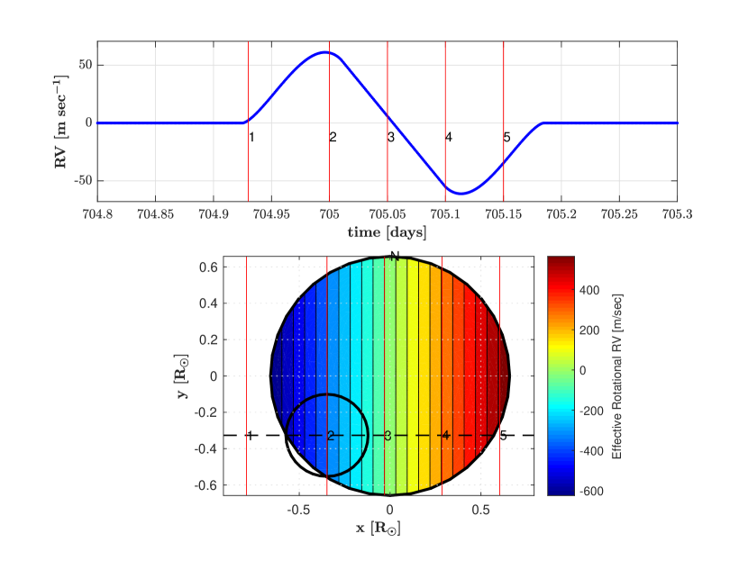
Figure 1: Bottom: A smaller body, denoted by the bold circle, moves across a larger star along the path given by the thick dashed line. The effective rotational radial velocity, ${\cal V}$, of the larger star (rotational period $P_{1}=35.1{\rm~{}days}$, $R_{1}=0.658~{}R_{\odot}$) is shown using the colors, with blue denoting large negative numbers and red denoting large positive numbers. The angles, defined in Equation (28), are $\Phi_{\rm rot}=90^{\circ}$, $\Theta_{\rm rot}=0^{\circ}$. The “North pole” of the star is marked with the letter “N”. There is no limb darkening and no differential rotation. Top: The R-M signal in ${\rm m~{}s^{-1}}$ is shown as a function of time. The numbers $1-5$ in the bottom panel are positions of the center of the smaller body, and correspond to those times at the top panel.

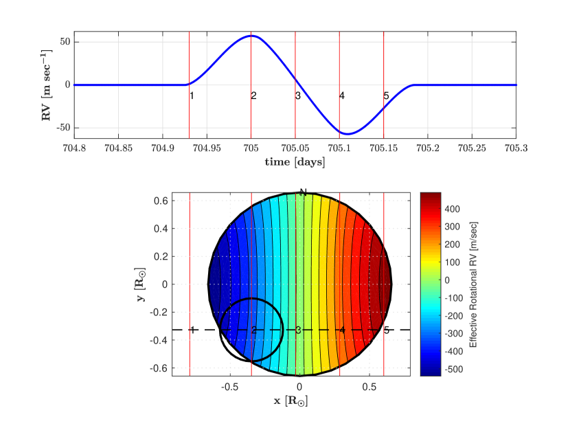
Figure 2: Similar to Figure 1, with no differential rotation, but with quadratic limb darkening ($c_{1}=0.77113,~{}~{}c_{2}=-0.050753$).

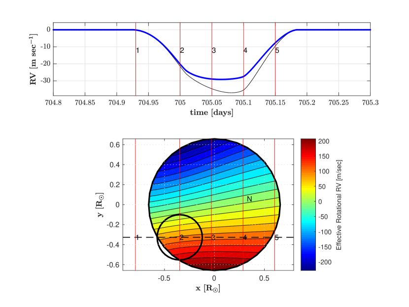
Figure 5: Similar to Figure 4, but with a misaligned rotation axis ($\Phi_{\rm rot}=30^{\circ}$, $\Theta_{\rm rot}=-80^{\circ}$). For comparison, the light black line in the top panel shows the R-M signal for a star with the same axial orientation but rotating as a rigid body (i.e. $\epsilon=0$).

For convenience we will refer to the quantity $v(x,y)I(\mu)\cos(\gamma)$ as the “effective rotational radial velocity”, ${\cal V}(x,y)$. To visualize how the R-M effect can change with limb darkening, with the change in orientation of the rotational axis, and with differential rotation, we computed ${\cal V}$ in a mock system in which a small star transits a much larger star (Figures 1-5). We start with the simple case (Figure 1) of no limb darkening, an aligned spin axis ($\Phi_{\rm rot}=90$, $\Theta_{\rm rot}=0$, meaning the star’s rotation axis is parallel to the y axis), and no differential rotation. In this case, the contours of ${\cal V}$ are vertical lines, hence the value of ${\cal V}$ at each point represents the true Doppler shift at that point. The R-M signal in this case is a symmetric “Z-wave”. We now add limb darkening (Figure 2). The contours of ${\cal V}$ now become symmetrically curved towards the rotation axis, hence, ${\cal V}$ is not a true Doppler shift any longer. Since $|{\cal V}|$ is symmetric about the rotation axis, the R-M signal is, likewise, symmetric. The third case (Figure 3) shows an aligned system with no limb darkening and with differential rotation. The contours of ${\cal V}$ are symmetrically curved in a manner similar to that of the second case. As before, the R-M signal is symmetric. When compared to the first case, we note that the amplitude of the R-M signal is smaller when differential rotation is included. The fourth case (Figure 4) shows an aligned system with both limb darkening and differential rotation. The ${\cal V}$ contours become curved to a greater extent than in the previous cases. However, since the symmetry of the vector field about the rotational axis remains, the R-M signal is, likewise, symmetric. When compared to the second case, the amplitude of the R-M signal is reduced. Finally (Figure 5), we show an example where the rotation axis of the star is misaligned with the orbit of the transiting body ($\Phi_{\rm rot}=30$, $\Theta_{\rm rot}=-80$). The ${\cal V}$ contours show no symmetry at all, and therefore the R-M effect exhibits no symmetry. When compared to a similar (misaligned) system with rigid body rotation, the difference between the R-M signals is quite noticeable.

4.3 The Computation and Accuracy of the Method

The computation of the light loss and the R-M effect through a transit involves the sum of integrals of simple functions (Equation 25). For the flux fraction, each limb darkening law has a vector of simple functions with components involving $\mu$ (e.g. $\mu^{0}$, $\mu^{1/2}$, $\mu^{1}$, etc., see Equations 13 through 17), and each of these functions of $\mu$ has a 1-form associated with it (Table 1). For the R-M effect, these simple functions involve $\mu$, $x$, and $y$ (e.g. $\mu^{2}x$, $\mu y$, etc.), and the associated 1-forms are also given in Table 1. Each 1-form used eventually leads to a definite integral that one would need to evaluate. When the integration arc is on the boundary of the back body (that is when $M=N$), $\mu=0$ and the 1-forms simplify greatly, leading to closed-form expressions for all of the definite integrals. When the integration arc is the boundary of the front body projected onto the back body (that is when $M<N$), the definite integrals associated with the $\mu^{0}$ and $\mu^{2}$ terms for the flux fraction and the $x$, $y$, $\mu^{2}x$, and $\mu^{2}y$ terms for the R-M effect (with no differential rotation) lead to definite integrals that can be evaluated in terms of a sum of simple functions. We give all of these closed-form expressions in Appendix E.

Apart from the specific cases given in Appendix E, the computation of the flux fraction and the R-M effect will involve definite integrals that need to be evaluated numerically, and we use Gaussian quadrature for this purpose.We can show, using standard techniques, that we can compute the definite integrals to any degree of precision desired. To do this, each integration arc is divided up into $K$ “panels” according to

$$\begin{aligned} K={\rm NINT}\big{[}2p(\varphi_{1}-\varphi_{0})+1\big{]}T_{\rm pan}\end{aligned}$$ (35)

where NINT is the “nearest integer” function, $T_{\rm pan}$ is an integer “tolerance” parameter, $\varphi_{0}$ and $\varphi_{1}$ are the starting and ending angles (in radians) of the arc, respectively, and where $p=R_{M}/R_{N}$ is the ratio of the front body’s radius to the back body’s radius. The code then employs Gaussian 4-point quadrature as the integration method for each panel. The error estimate for the computation of the definite integrals that give the fractional flux (Equation 19) is based on the asymptotic error formula for Composite Gaussian Integration and on the Aitken extrapolation method for linearly convergent sequences (Atkinson, 1989). The asymptotic error formula for Gaussian 4-point quadrature depends on the differentiation order of the integrand. Equation D7 in appendix D implies that the order will always be at least 1. In this case the asymptotic error formula for Composite Gaussian Integration is $O(h^{2})$ where $h$ is the panel width. If we now define a sequence of fractional fluxes with the panel length reduced by half ($T_{\rm pan}$ doubled) for successive members, this sequence will converge linearly with the ratio of successive differences being 0.25 or less. We can then apply the Aitken extrapolation to obtain a much better approximation to the sequence limit. The difference between the sequence and the extrapolated values provides the error estimate. To illustrate this, we apply the process to the example containing four bodies which we discuss in Appendix A. The values for each step in the error estimation process are shown in Table 2. The first panel in Table 2 lists the flux fractions for all but the first (unobscured) body for 7 different values of the tolerance $T_{\rm pan}$. Following the Aitken extrapolation algorithm, we compute successive flux differences for each of the bodies. We then compute the ratio of the differences. Note that these ratios for each body are almost constant (property of linear convergence) and they are all less than 0.25. Finally, we apply the Aitken formula resulting in the extrapolated flux. Comparing the flux to the extrapolated flux provides the error estimate. In this case every doubling of the subintervals results in an error reduction of a factor of $\sim$ 0.18, the ratio of the differences. When the tolerance is $T_{\rm pan}=128$ the error in the fractional flux is $\approx 10^{-12}$ or better. In the discussion that follows we will assume that light curves computed using $T_{\rm pan}=128$ are “exact”.

The quadrature error one gets for a given number of panels $K$ depends on the rate of convergence of the process which, in turn, depends on the bounds of higher-order derivatives of the integrand. When the bounds are not available (for example, owing to singularities), higher-order convergence might not occur. An instructive example is the simple integral

$$I=\int_{a}^{1}\sqrt{x}dx={\frac{2}{3}}\left(1-a^{3/2}\right)\quad\rm{for}\,\,0\leq a<1$$

The first derivative of the integrand has a singularity at $x=0$. When $a=0.1$, 6 panels are needed to give a quadrature error of less than $10^{-8}$, using 4-point Gaussian quadrature. As $a\rightarrow 0$, the number of panels required to keep the same accuracy increases. For example, when $a=0.05$, 11 panels are needed to get an error less than $10^{-8}$, and when $a=0.01$, the number of panels required is $K=34$. When our simple integral becomes

$$I=\int_{a}^{1}{x}^{3/2}dx={\frac{2}{5}}\left(1-a^{5/2}\right)\quad\rm{for}\,\,0\leq a<1$$

the singularity at $x=0$ does not occur until the second derivative of the integrand. In this case, the number of panels required to get a quadrature error of $10^{-8}$ becomes $K=4$, 6, and 12 when $a=0.1$, 0.05, and 0.01, respectively. This exercise will be useful in the following discussion.

We have a code that can compute the flux fractions for any number of mutually overlapping bodies to any degree of desired precision by using a large number of quadrature panels for each arc on the visible boundaries. In most practical applications, a fractional precision in the models down to $\approx 10^{-15}$ is unnecessary. Depending on the available observational data, one might only need model light curves with fractional precisions of $\approx 10^{-6}$ to $10^{-8}$. In addition, in most cases only two overlapping bodies need to be considered at any given time. Given this fact, we can make some modifications in the algorithm to increase the performance while giving reasonably small quadrature errors. There are four types of changes we can make, and we discuss these below.

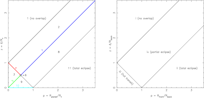
Figure 6: Left: The $(p,z)$ plane showing the various cases used to compute eclipse events in the Mandel & Agol algorithm, where $p$ is the ratio of the radii and $z$ is the distance between the centers, normalized to the radius of the body in back. Regions 4, 5, 7, and 10 are lines and region 6 is a single point. Different functions may need to be evaluated for different regions. In the MA2002 notation, the “planet” is always the body in front and the “star” is always the body in back. Right: The $(p,z)$ plane showing the four cases used to compute eclipse events in our algorithm. The only distinction between case iii and iv is the number of function evaluations used. For clarity we have used $R_{\rm front}$ as the radius of the body closer to the observer (called $R_{M}$ in the text), and $R_{\rm back}$ to denote the radius of the more distant star (called $R_{N}$ in the text).

When working with only two bodies, the two important parameters that determine the flux fraction are the ratio of the radii of the two objects and the separation of the centers in the POS. In the notation of MA2002 the parameter $p$ is given as $p\equiv R_{\rm planet}/R_{*}$, where $R_{\rm planet}$ is always the radius of the front body and $R_{*}$ is the radius of the back body. In addition, MA2002 define a parameter $z\equiv\delta/R_{*}$, where $\delta$ is the separation of the centers in the POS. In our notation these quantities are $p\equiv R_{M}/R_{N}$ and $z\equiv\delta/R_{N}$. MA2002 partition the ($p,z$) plane into 11 regions (see Figure 6), and these will be discussed in greater detail below. For our discussion, we have four regions as shown in Figure 6, two of which are trivial: (i) when $z>p+1$ there is no overlap (this is Region 1 in MA2002); (ii) when $z<p-1$ we have a total eclipse (this is Region 11 in MA2002); (iii) when $z\leq 1-p$ we have a full transit (this area contains Regions 3, 4, 5, 6, 9, and 10 in MA2002); and (iv) when $z>1-p$ and $p-1\leq z\leq p+1$ we have a partial eclipse (this area contains Regions 2, 7, and 8 in MA2002).

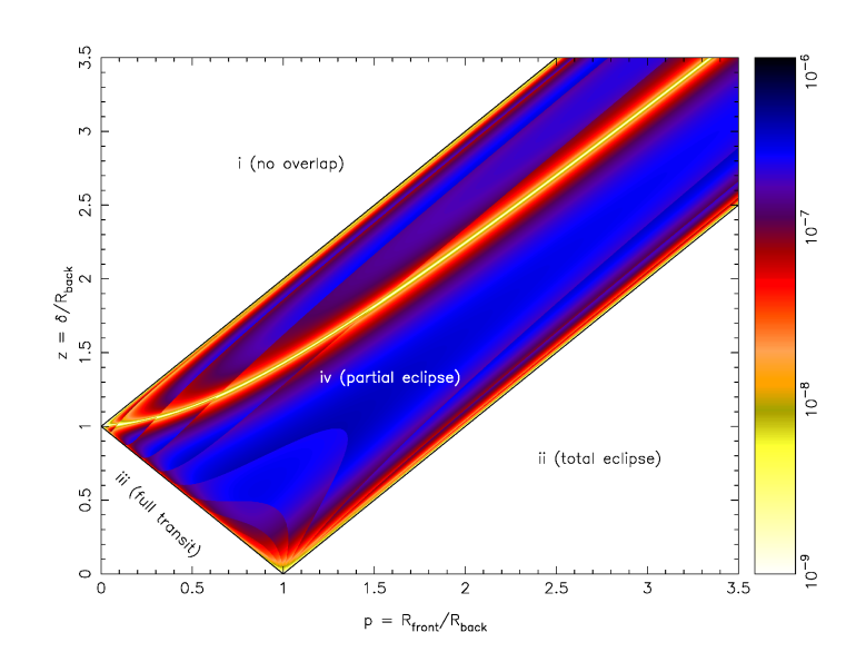
Figure 7: The quadrature error for the definite integral associated with the linear term in the limb darkening law over the $(p,z)$ plane. The darker colors represent errors on the order of a few parts per million. Errors below $10^{-9}$ are given as white.

We begin the algorithm refinement by first getting some idea of the quadrature errors when the number of quadrature panels is small. We use the quadratic limb darkening law with coefficients of 0.6 and 0.2. We divide up the ($p,z$) plane into a $2880\times 2880$ grid between 0.0 and 3.5 along each axis. At each point in the grid we compute the flux fraction using a tolerance of $T_{\rm pan}=2$ and $T_{\rm pan}=128$ and 4-point integration, and find the absolute value of the difference between the two flux fractions. We adopt this difference as a measurement of the quadrature error. Figure 7 shows a color map of the results. With two notable exceptions, the quadrature errors are on the order of a few times $10^{-7}$, where the out-of-eclipse flux is normalized to unity. The first exception is the triangle in the lower left of the diagram where the errors are less than $\approx 10^{-10}$. This is case (iii), discussed above where there is a full transit. Here the front body does not touch the limb of the back body (as seen on the POS), and the quantity $\mu$ is always greater than zero along the integration path. Higher-order derivatives of the integrands for the $\mu^{1/2}$, $\mu^{1}$ and $\mu^{3/2}$ terms will have factors of $\mu$ to various powers in the denominators, but since $\mu>0$ always, the higher-order derivatives will not suffer from singularities and hence the rate of convergence of the integration will be very high. On the other hand, when we consider case (iv) discussed above (e.g. a partial eclipse), the shadow boundary of the body in front will intersect the limb of the body in back. Thus, generally speaking, there will be some of the higher-order derivatives that will have a singularity when $\mu=0$, thereby slowing convergence. The second exception where the errors are smaller occurs along the curve described by $z=\sqrt{p^{2}+1}$. As we can see from Figure 7, the errors are $\approx 10^{-9}$ along this curve. One can show that along this curve, the integrand is effectively multiplied by a factor of $\mu^{2}$, which gives us two more higher-order derivatives before singularities occur. As a result, along this curve the convergence is faster and the errors are much smaller.

Now that we have some baseline-level estimate of the number of function evaluations that are required to get a reasonably small quadrature error, our first improvement to the algorithm involves using higher-order Gaussian quadrature. The number of function evaluations required to numerically compute the definite integrals would be $N_{\rm op}=4K$ for 4-point Gaussian quadrature and $K$ panels. Alternatively, one could use $(4K)$-point Gaussian quadrature and one panel to evaluate the definite integrals using the same number of function evaluations. The application of the Aitken extrapolation technique to evaluate the quadrature error for these high order quadrature cases is less straightforward since the order changes. Fortunately we can always use the difference between a model with a given tolerance and the same model computed using $T_{\rm pan}=128$ (or higher), and 4-point integration to get a good estimate of the quadrature error since the latter model can be shown to be very nearly exact. We have found from numerical experiments that using a higher order Gaussian quadrature over one panel always produces smaller errors than using 4-point Gaussian quadrature and $K$ panels, when the number of function evaluations is the same for both. This result is a consequence of the fact that the error formulae for Gaussian integration involve higher-order derivatives of the integrand and various constant coefficients, and while the derivatives of the integrands may suffer from singularities past the first or second order (thereby slowing convergence), the values of the constant terms do decrease with increasing order.

Thus, for our first modification to the algorithm, we set the number of operations as

$$\begin{aligned} N_{\rm op}={\rm NINT}\bigg{\{}\big{[}3.7p(\varphi_{1}-\varphi_{0})+1\big{]}T_{\rm op}\bigg{\}}\end{aligned}$$ (36)

where the meaning of the variables are the same as in Equation 35. The factor of 3.7 was arrived at through numerical experimentation. Also note that in this case, the tolerance parameter $T_{\rm op}$ is not necessarily an integer. Once we have the number of operations set, $N_{\rm op}$-point Gaussian quadrature is used for a single panel, up to order 64. If the number of desired operations exceeds 64, then the integration arc is subdivided with the requirement that the quadrature order is the same for each subarc and is as large as possible without exceeding 64. In addition, we set the minimum value of $N_{\rm op}$ to 8.

Our second modification to speed up the routine targets values of $p$ and $z$ where there is a full transit (that is, when $z\leq 1-p$). As discussed above, the quadrature errors there are very small owing to the properties of the higher-order derivatives of the integrand. Since the convergence in this region is relatively fast, we can get by with fewer overall function evaluations, $N_{\rm op}$, and we start with $N_{\rm op}=8$. Generally speaking, the quadrature errors are the smallest when both $p$ and $z$ are small, and increase as one moves up diagonally in the region. Consequently, we define triangles with vertices given by $p=0$ and $z=1$, $p=1$ and $z=0$, and $p=p_{0}$ and $z=z_{0}$ (where $p_{0}=z_{0}$). For a given point $(p,z)$, $N_{\rm op}$ is increased by 1 when the following conditions are met: if it is inside the triangle with a vertex of (0.25,0.25), if that point is inside the triangle with vertex (0.35,0.35), if it’s inside the triangle with vertex at (0.40,0.40) and, finally, if the point is between the lines given by $z=0.997-p$ and $z=1-p$.

The third modification we can make to increase the algorithm performance is for the case where there are only two bodies and only the flux fraction is required. The co-ordinate system in the POS can be rotated in such a way so that the center of the front body lies on the $x$-axis. In that case, the starting and ending angles of the arc will be symmetric about the $x$-axis. For example $\varphi_{0}=330^{\circ}$ and $\varphi_{1}=390^{\circ}$, or $\varphi_{0}=170^{\circ}$ and $\varphi_{1}=190^{\circ}$. In cases like these, we can integrate over half of the arc (thereby using half the number of function evaluations) and multiply the quadrature sum by 2 to get the final flux fraction. This modification won’t work when computing the R-M effect, as both the $x$ and $y$ co-ordinates of the center of the body in front are important, which makes the axis rotation impossible.

Similarly to the third modification, the final one applies to the case of having only two bodies. Many of the procedures described in Appendix A to construct the arcs in the general routine for $\cal{N}$ bodies are not necessary when there are only two bodies. For example checking for arc intersections or computing the shadow boundary. In addition, having to store only the angles greatly simplifies the code. This streamlined version of the routine is about 10% faster than the general routine called when ${\cal N}=2$. It is straightforward to decide whether to call the general routine or the two-body routine based on the sizes of the bodies and the distances between them.

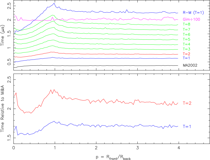
Figure 8: Top: The time in microseconds needed to compute a flux fraction as a function of the radius ratio $p$. The black line is for the Mandel & Agol occultquad routine, the bottom curves are for $T_{\rm op}=1$ to $T_{\rm op}=8$ in steps of 1, the magenta curve is for the Giménez routine (which includes the R-M effect) where the times were divided by 100, and the top blue curve is for the R-M effect and flux fraction for $T_{\rm op}=1$. Bottom: The ratio of the $T_{\rm op}=1$ and $T_{\rm op}=2$ times relative to the MA2002 occultquad routine.

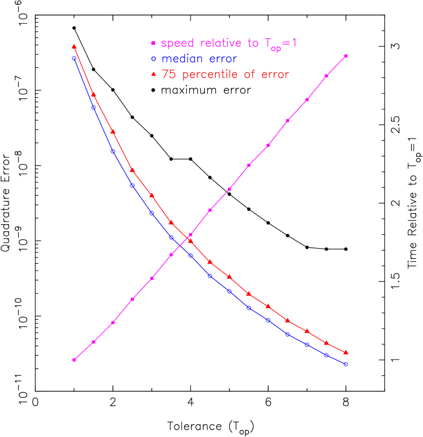
Figure 9: The quadrature errors (left-hand scale) and relative algorithm speed (right-hand scale) for the computation of the flux fraction as a function of the tolerance $T_{\rm op}$. The various curves show the maximum error (black filled circles), the 75 percentile error (red triangles), and the median error (blue open circles). The magenta filled squares give the speed relative to the $T_{\rm op}=1$ models.

We have performed extensive tests to measure the speed of our routines. For a given value of $p$, the value of $z$ was varied from $z=p-1$ to $z=p+1$ in steps of $10^{-6}$ (when $p<1$ the lower bound on $z$ is zero) and a flux fraction was computed for each $z$ using the quadratic law. The time required to compute these flux fractions was measured using the FORTRAN function cpu_time(). These tests were done on a workstation with an Intel Xeon W-2155 CPU running at 3.30 GHz using the Portland Group FORTRAN compiler version 18.4 with the -fast optimization flag. Figure 8 shows the results. For a given tolerance, the time required to compute a flux fraction rises from small values of $p$, reaches a peak near $p=1$, then drop off modestly thereafter. Past $p\approx 3$, the curves are flat. When $T_{\rm op}=4$, the time to compute a single flux fraction is about one microsecond. Figure 9 shows the time required relative to $T_{\rm op}=1$ for values of $T_{\rm op}$ ranging from 1 to 8 in steps of 0.5. The time vs. tolerance curve is nearly linear, and the slope is modest since models with $T_{\rm op}=8$ take about three times longer than models with $T_{\rm op}=1$. For other limb darkening laws, the times required relative to the quadratic law are 0.93 for the linear law, 1.55 for the logarithmic law, and 1.89 for the square root law.

When computing the R-M effect, some numerical experimentation has shown that more function evaluations are required to ensure the quadrature error is less than $\approx 0.1{\rm m~{}s^{-1}}$. The multiplier in Equation 36 is 12.0 instead of 3.7. Also, the convergence of the Gaussian quadrature for $p>1$ near the onset of total eclipses is relatively slow, so the value of $N_{\rm op}$ is increased by 4 when $p>1$ and $z<\sqrt{p(p+1)}$ (these conditions were arrived at after the inspection of many error maps). When $T_{\rm op}=1$, it takes about 3.6 times longer to compute a flux fraction along with the R-M correction compared to computing the flux fraction alone.

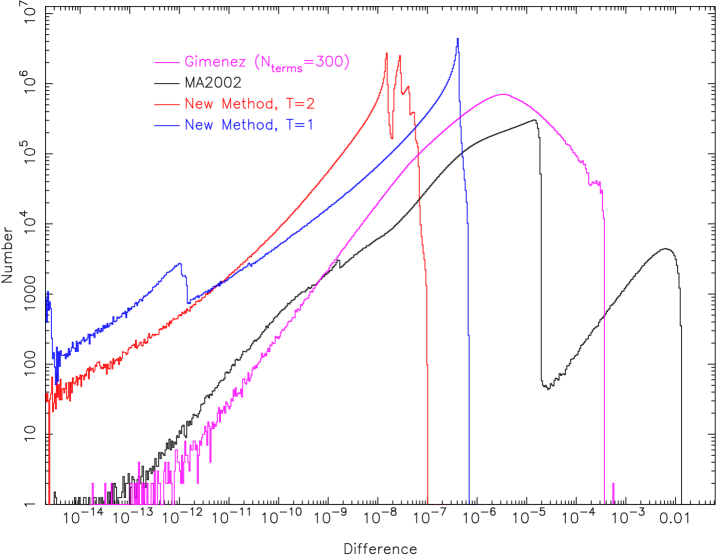
Figure 10: The frequency distributions for the quadrature errors associated with the flux fraction computation for the quadratic limb darkening law for values of the radius ratio $p$ between 0 and 100. The curves are for the occultquad routine of MA2002 (black), the Giménez (2006a) routine (magenta), our new method with $T_{\rm op}=1$ (blue) and our new method with $T_{\rm op}=2$ (red).

To fully characterize the quadrature errors, we computed flux fractions for $5\times 10^{7}$ randomly selected points in the $(p,z)$ plane for $0<p<100$ and $p-1<z<p+1$ (when $p<1$ the lower bound on $z$ is of course zero). The flux fractions were computed using the quadratic law with coefficients of 0.6 and 0.2, for values of $T_{\rm op}$ ranging from 1 to 8 in steps of 0.5, and for $T_{\rm pan}=128$. We also computed models using $T_{\rm op}=2$ for each of the linear, square root, and logarithmic limb darkening laws. Using the $T_{\rm pan}=128$ model as the reference, we computed the quadrature errors for the other models. Figure 10 shows the frequency distributions for the $T_{\rm op}=1$ and $T_{\rm op}=2$ quadratic law cases. When $T_{\rm op}=1$, the maximum quadrature error is $6.72\times 10^{-7}$, and when $T_{\rm op}=2$, the maximum quadrature error is $1.00\times 10^{-7}$. The histograms for the $T_{\rm op}=2$ models with the other limb darkening laws look very similar to the histogram for the quadratic law. The maximum errors (for $T_{\rm op}=2$) are $1.13\times 10^{-7}$ for the square root law, $1.00\times 10^{-7}$ for the logarithmic law, and $5.82\times 10^{-8}$ for the linear law.

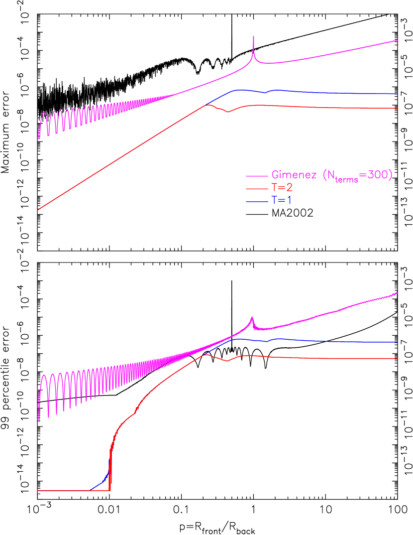
Figure 11: The maximum quadrature error (top) and the 99 percentile error (bottom) for the computation of the flux fraction using the quadratic limb darkening law as a function of the radius ratio $p$. The curves are for the MA2002 occultquad routine (black), the Giménez (2006a) routine (magenta), our new method with $T_{\rm op}=1$ (blue) and our new method with $T_{\rm op}=2$ (red).

Figure 11 shows how the quadrature errors depend on the ratio of radii $p$. To generate this plot, we took 3000 values of $\log p$ ranging between $-3.0$ and 2.0 in equal steps. For a given bin centered on a particular value of $p$, 100,000 values of $z$ were randomly chosen in the appropriate range, and the quadrature errors were found for all of the cases. Then the maximum quadrature error and the 99 percentile error in that bin were found. For planet transits (i.e. small $p$), the maximum quadrature error is $10^{-8}$ or smaller. When the value of $p$ is around $p=1$, the quadrature errors flatten out, and they never exceed the thresholds mentioned previously. Finally, Figure 9 shows how the errors change as the tolerance parameter $T_{\rm op}$ changes. As one might expect, the maximum quadrature error decreases as $T_{\rm op}$ increases. Furthermore, the median of the error distribution is usually smaller than the maximum error by an order of magnitude or more.

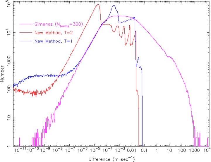
Figure 12: The frequency distributions for the quadrature errors in ${\rm m~{}s^{-1}}$ associated with the R-M computation for the quadratic limb darkening law for values of the radius ratio $p$ between 0 and 100. The curves are for the Giménez (2006a) routine (magenta), our new method with $T_{\rm op}=1$ (blue) and our new method with $T_{\rm op}=2$ (red).

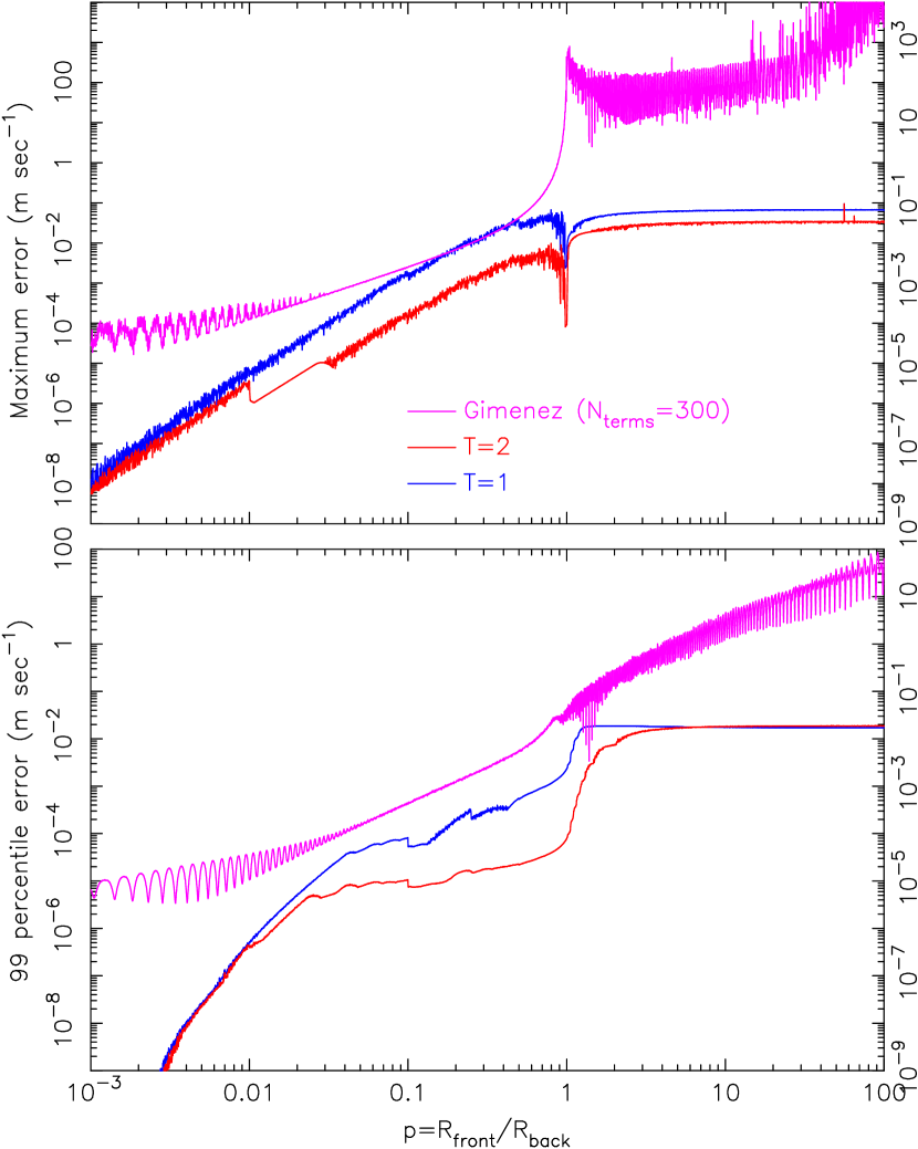
Figure 13: The maximum quadrature error (top) and the 99 percentile error (bottom) for the computation of the R-M effect using the quadratic limb darkening law as a function of the radius ratio $p$. The curves are for the Giménez (2006b) routine (magenta), our new method with $T_{\rm op}=1$ (blue) and our new method with $T_{\rm op}=2$ (red).

For the computation of the R-M effect, we have at least three parameters. At a minimum, we need the ratio of radii $p$ and the relative $x$ and $y$ co-ordinates of the two bodies on the POS. For simplicity we consider cases when $\Phi_{\rm rot}=90^{\circ}$ and $\Theta_{\rm rot}=0$. We computed the R-M effect for $5\times 10^{7}$ cases with $0<p<100$ and relative $x$ and $y$ co-ordinates appropriate for each $p$ for $T_{\rm op}=1$ and $T_{\rm op}=2$. We used the quadratic limb darkening law with coefficients of 0.6 and 0.2, and assumed a rotation period of 10 days and a radius of $1\,R_{\odot}$ for the back body. Figure 12 shows the distribution of the quadrature errors (in ${\rm m~{}s^{-1}}$). When $T_{\rm op}=1$, the maximum quadrature error is $\sim 0.067~{}{\rm mm~{}s^{-1}}$. Figure 13 shows the maximum quadrature error and the 99 percentile error as a function of $p$, where the same procedure used to make Figure 11 was used. For planet transits where $p\lesssim 0.1$ the quadrature errors are less than about $10^{-3}~{}{\rm m~{}s^{-1}}$. When $p>1$, the maximum quadrature errors are around $10^{-2}{\rm m~{}s^{-1}}$.

When working with three or more bodies, we no longer have a simple plane in which we can map out the uncertainties. However, all of the arcs in multibody cases are subarcs of all pairwise two-body cases. Thus, all of the integrands are the same, although the integration intervals might be smaller and/or broken into pieces. Therefore, the behavior of the quadrature should be similar. In many of the multi-body cases the integrand does not change sign from the two-body cases, and this would result in the quadrature error of a subarc being roughly the same as the two-body quadrature error.

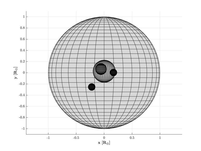
Figure 14: The spatial configuration of a mock 5-body system discussed in §4.3, shown near the time of the transit of four smaller bodies across the largest body.

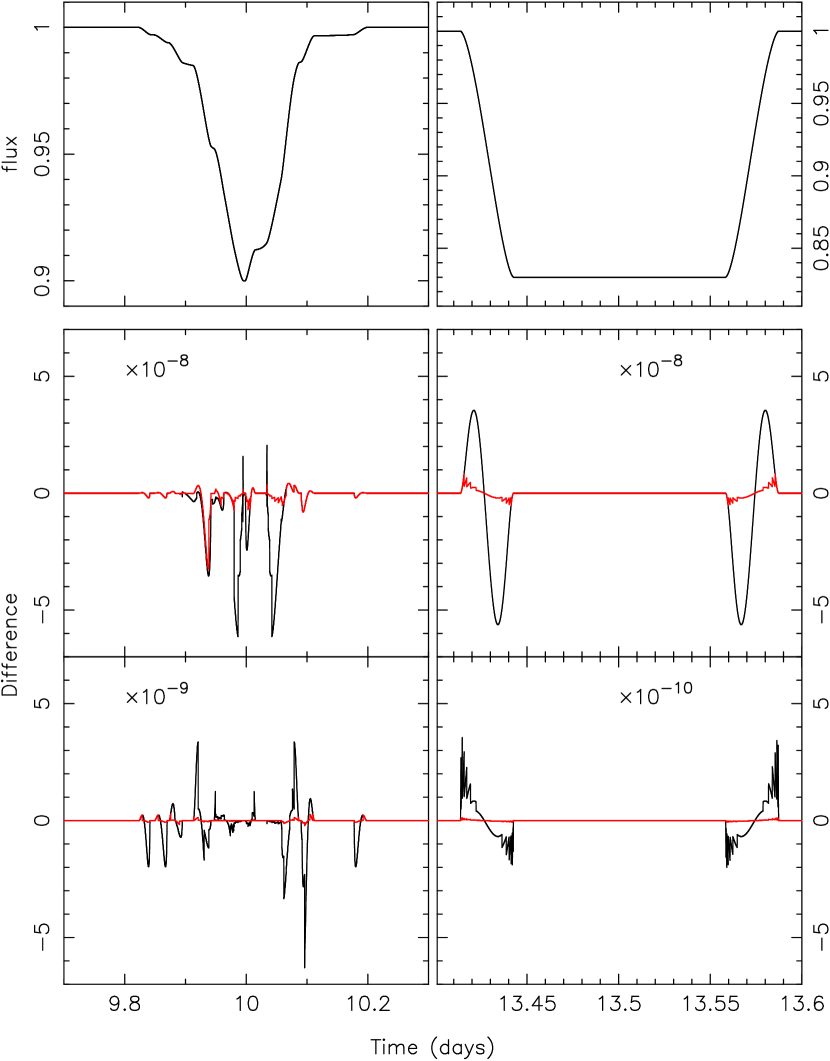
Figure 15: Top: The light curve of a mock five-body system during the transit of the four smaller bodies across the largest body (left), and during a total eclipse of the second body by the first (right). Middle: The difference between the nominal light curve made with $T_{\rm pan}=128$ and the light curves made with $T_{\rm op}=1$ (black), and $T_{\rm op}=2$ (red). Bottom: The difference between the nominal light curves with $T_{\rm pan}=128$ and the light curves made with $T_{\rm op}=4$ (black), and $T_{\rm op}=8$ (red)

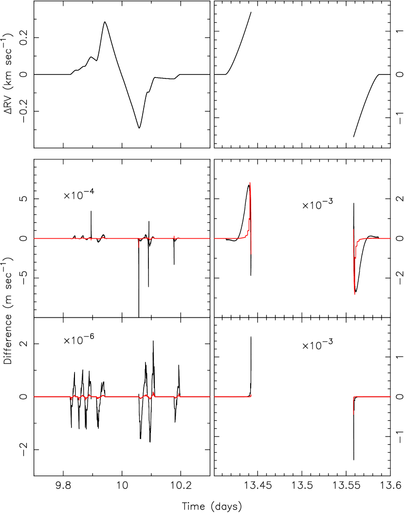
Figure 16: Top: The R-M effect of a mock five-body system during the transit of the four smaller bodies across the largest body (left), and during a secondary eclipse (right). The orbital motion of the star has been removed. Middle: The difference between the nominal R-M curve with $T_{\rm pan}=128$ and the R-M curve with $T_{\rm op}=1$ (red), and $T_{\rm op}=2$ (black) The units of the differences are ${\rm m~{}s^{-1}}$, and the curves have been scaled as indicated. Bottom: The difference between the nominal R-M curve and the R-M curve with $T_{\rm op}=4$ (black), and $T_{\rm op}=8$ (red).

To illustrate the errors and how the errors decrease with increasing tolerance, we computed light curves of a mock 5 body system (see Figure 14) with masses of $M_{1}=0.8\,M_{\odot}$, $M_{2}=0.2\,M_{\odot}$, $M_{3}=5\times 10^{-4}\,M_{\odot}$, $M_{4}=4\times 10^{-4}\,M_{\odot}$, and $M_{5}=2.5\times 10^{-4}\,M_{\odot}$, radii of $R_{1}=1.0\,R_{\odot}$, $R_{2}=0.2\,R_{\odot}$, $R_{3}=0.1\,R_{\odot}$, $R_{4}=0.0625\,R_{\odot}$, and $R_{5}=0.0625\,R_{\odot}$, and fluxes of $F_{1}=0.80$, $F_{2}=0.17$, $F_{3}=0.01$, $F_{4}=0.01$, and $F_{5}=0.10$. The initial orbital parameters were circular but a full integration of the laws of motion advanced the bodies (for a detailed description of our integration see Welsh et al. (2015) and Hairer & Hairer 2002). The initial periods were $P_{1}=7$ days, $P_{2}=70$ days, $P_{3}=210$ days, and $P_{4}=500$ days. The orbital inclinations were close to $90^{\circ}$, and the nodal angles were close to $0^{\circ}$. The initial positions of the bodies were such that the four smaller bodies all transited the largest star near day 10.0. At this time we have a complex pattern of arcs describing the visible boundary of the most distant star, and this pattern rapidly changes before and after this time. The model light curves were computed (assuming quadratic limb darkening) with tolerances of $T_{\rm op}=1,2,4,8$, and $T_{\rm pan}=128$. Figure 15 shows a close-up of the multi-body transit event at day 10, as well as a close-up of a total eclipse of the second body at day 13.5. We plot the curves showing the differences between the $T_{\rm pan}=128$ curve and the other curves. For $T_{\rm op}=1$, the errors in the computed fluxes are a few parts in $10^{7}$. As the tolerance gets larger, the differences get smaller, as expected. Figure 16 shows the R-M curves for the multi-body event at day 10, and for a secondary eclipse at day 13.5, assuming synchronous rotation, $\Phi_{\rm rot}=90^{\circ}$, and $\Theta_{\rm rot}=0^{\circ}$. For the syzygy event near day 10, the quadrature errors are smaller than $10^{-3}~{}{\rm m~{}s^{-1}}$ for $T_{\rm op}=1$, and considerably smaller than that for $T_{\rm op}=2$, 4, and 8. The quadrature errors are somewhat larger just before the onset of the total secondary eclipse owing to the lower differentiability order near there, which slows the convergence of the quadrature process. Even so, the spikes there are at the level of a few times $10^{-3}~{}{\rm m~{}s^{-1}}$, which seems adequate for most practical applications.

5 Comparison with Other Methods

For comparison purposes, we have a direct implementation of the MA2002 occultquad routine for quadratic limb darkening. The accuracy of this routine is not adjustable. We also wrote our own routine to implement the Giménez (2006a) method for computing the flux fraction for the quadratic limb darkening law and the Giménez (2006b) method for computing the R-M effect, which also uses the quadratic limb darkening law. The accuracy of this routine is adjustable by specifying the parameter $N_{\rm terms}$, which is the number of terms in the polynomial expansions (namely Equation 11 from Giménez 2006a and Equation 11 from Giménez 2006b). A larger number of polynomial terms provide more accurate light curves but, obviously, at the expense of longer computation times. We typically use $N_{\rm terms}=300$.

We performed speed tests of these two algorithms using the same procedure as above, and the results are shown in Figure 8. When $p\gtrsim 0.5$, occultquad requires about 0.36 microseconds to compute a flux fraction, which is about 1.7 and 2.1 times faster compared to our method with $T_{\rm op}=1$ and $T_{\rm op}=2$, respectively. The Giménez routine with $N_{\rm terms}=300$ is significantly slower as it requires about 200 microseconds to compute a flux fraction along with the R-M effect, which is $\approx 80$ times slower than our R-M routine using $T_{\rm op}=1$. We note, however, that within the workings of the our photodynamical code, the time required to compute the flux fraction, with any of the methods, is relatively small compared to the time required for integrating the Newtonian equations of motion, and computing the fitness. For example, in the case of Kepler-16, running the DEMCMC-based optimizer is only a factor of 2 slower than running the same code with occultquad or our routine. In other words, in the context of our full photodynamical modeling, a factor of a few in the speed difference of the flux fraction routine is not really noticeable.

We also characterized the quadrature errors for these two routines using the same procedures described above. Figure 10 shows the results. The quadrature errors for the Giménez routine are smaller than a few times $10^{-4}$. The mode of the error distribution for the occultquad routine is around $10^{-5}$. In addition, this distribution has a small extension to errors of up to about 0.01. Figure 11 shows how the quadrature errors depend on the ration of radii $p$. For planet transits (i.e. for small $p$), the 99 percentile quadrature errors for occultquad and for the Giménez routine are smaller than $10^{-6}$, and in most cases considerably smaller. However, the maximum error for occultquad is about $10^{-5}$ when $p=0.1$. Furthermore, the maximum error goes up with increasing $p$ and reaches $\sim 0.01$ when $p=100$. Also note a rather significant spike in the occultquad curve near $p=0.5$, where the 99 percentile error is about 0.001 and the maximum error reacher $\sim 0.01$. The quadrature errors for the Giménez routine also grow with increasing $p$, and there is also a modest spike, although it occurs at $p=1$ instead of $p=0.5$. We note that we do have the option of increasing $N_{\rm terms}$ in order to reduce the quadrature errors.

We can see from Figure 11 that for a given value of the ratio of radii $p$, the 99 percentile quadrature error for the occultquad routine is usually two or three orders of magnitude smaller than the maximum quadrature error. This suggests that there is a small but significant tail in the quadrature error distribution that extends to relatively large values. To see why that is, we refer again to Figure 6, which shows the $(p,z)$ plane, where $p\equiv R_{\rm planet}/R_{*}$ in the Mandel & Agol notation (in our notation $p\equiv R_{M}/R_{N}$), and where $z\equiv\delta/R_{\ast}$ in the Mandel & Agol notation (in our notation $z\equiv\delta/R_{N}$) with $\delta$ being the separations of the centers on the POS. In the MA2002 occultquad routine, the $(p,z)$ plane is divided up into 11 regions as indicated in the figure. For example, region 1 is where no transit events occur. In region 2 the planet disk lies on the limb of the star but does not cover the center of the stellar disk. Regions 4, 5, 7, and 10 are lines in the plane, and region 6 is a single point. For a given eclipse or transit event, the $p$ co-ordinate is fixed, while the $z$ co-ordinate changes with time. Therefore, as an eclipse or transit event is computed in time, the locations of the $(p,z)$ points “move” along vertical lines in the plane. As they do so, these points might pass through more than one region, and the transitions between the regions might not be smooth. Depending on where in the plane a particular $(p,z)$ point is located, there are different functions to evaluate the flux fraction when computing the flux deficit. Note that in our method and the method of Giménez, the same functions are evaluated regardless of where one is in the $(p,z)$ plane.

Consider an eclipse event that is in region 8 (planet covering the center and limb of the stellar disk) at the closest approach of the centers. Region 7 (planet’s disk touches the stellar center) and region 2 (planet lies on the limb of the star but does not cover the center of the stellar disk) will have to be crossed as the objects move apart. When calculating the flux deficit in regions 2 and 8 one has to evaluate a function, $\lambda_{1}$ (MA2002 Table 1), the last term of which is:

$$\lambda_{1}=\frac{1}{9\pi\sqrt{pz}}\bigg{[}\ldots-\frac{3q}{a}\Pi\left(\frac{a-1}{a},k\right)\bigg{]}$$ (37)

where $a=(z-p)^{2}$ and $q=p^{2}-z^{2}$, and where $\Pi$ is the complete elliptic integral of the third kind. Note that

$$\frac{q}{a}=\frac{p+z}{p-z}$$ (38)

so as $z\rightarrow p$, $q/a\rightarrow\infty$. Likewise, the argument of $\Pi$ also approaches $\infty$ as $z\rightarrow p$. This probably means that the complete elliptic integral goes to 0, thus as $z\rightarrow p$, the last term of $\lambda_{1}$ approaches $\infty\times 0$, (which is indeterminate). Hence, an asymptotic form of the function $\Pi$ would be required to determine what should happen at this limit. In any event, the flux values on either side of the point in time when the planet’s limb touches the stellar center might not line up smoothly. Indeed, Ofir et al. (2018) noted difficulties in their models of transit time variations which require time derivatives of finely-sampled transit profiles.

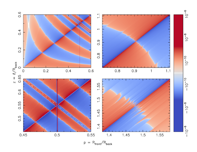
Figure 17: Color maps of the MA2002 occultquad quadrature errors in four small regions in the $(p,z)$ plane. Red colors indicate a positive difference (occultquad flux is larger than the $T_{\rm pan}=128$ flux fraction) and blue colors indicate a negative difference. Darker colors denote more extreme differences. The errors are the largest along the lines $z=p$ and $z=1-p$, and also nearby the vertical line $p=0.5$.

Figure 17 shows a color map of the occultquad quadrature errors in four small areas of the $(p,z)$ plane. The quadrature errors are generally quite small, except along the lines $z=p$ and $z=1-p$ (which are boundaries between various regions) and the vertical line $p=0.5$. Given that regions 4, 5, and 7 are lines in the plane and region 6 is a single point, these regions will never be reached in an actual calculation. The boundaries are “fattened” inside the occultquad routine by multiplying the terms of $z+p$, $z-p$, and $1-p$ by constants equal to $10^{-4}$ or 1.0001. Large quadrature errors would occur if a point in the $(p,z)$ plane that is nearby a boundary is assigned to the wrong region.

In the tests that are summarized in Figure 11, we have effectively computed eclipse profiles for an excessively large number of points in time or orbital phase, and with a large number of points problem areas in the $(p,z)$ plane will be encountered. In practice, of course, one would use perhaps a few dozen to a few hundred points per eclipse or transit event when modeling actual observational data. So, in cases like these, how likely are we to encounter these problem areas in the $(p,z)$ plane? To answer this, we computed light curves using the ELC code of Orosz & Hauschildt (2000), which has implementations of all three methods under discussion here. This makes it easy for us to make direct comparison of light curves computed using the various methods for cases that have no more than two overlapping bodies at any given time.

We start with the triple system KIC 10319590 as our first test case. This system is one of the more interesting eclipsing binaries discovered by the Kepler mission as the eclipses disappeared over a $\approx 600$ day span near the start of the mission, owing to the influence of a third body companion (Orosz, 2015). Thus we have a convenient way to compute eclipses with different impact parameters. We computed the light curve over a 686 day span using the new method with $T_{\rm op}=2$, the new method with $T_{\rm pan}=128$, the occultquad routine, and our Giménez routine with $N_{\rm terms}=300$. For this demonstration we set the initial inclination of the binary to $89.6^{\circ}$ instead of its best-fitting value of $88.84^{\circ}$ in order to produce deeper eclipses. Figure 18 shows the light curve computed with $T_{\rm pan}=128$, and the difference between that light curve and the three others. The maximum difference between the $T_{\rm op}=2$ light curve and the $T_{\rm pan}=128$ light curve is about $2\times 10^{-8}$. The maximum difference between the $T_{\rm pan}=128$ light curve and the Giménez light curve is about $4\times 10^{-6}$. Finally, the maximum difference between the $T_{\rm pan}=128$ light curve and the occultquad light curve is about $10^{-5}$. Note that the spikes in that difference curve extend to much later times than the spikes in the difference curve for the Giménez model do. Figure 19 shows a close-up on the difference curves for the first primary eclipse and a (much shallower) primary eclipse near day 349. We see that the maximum difference between the $T_{\rm pan}=128$ model and the Giménez model of $4\times 10^{-6}$ is near the times of second and third contact. The maximum difference between the $T_{\rm pan}=128$ model and the occultquad model occurs near the time when the secondary star is about to pass over the center of the primary star (that is when $z=p$). Thus there will be transition from one region to another one in the $(p,z)$ plane.. At some time around day 320, owing to the precession of the binary caused by the tertiary companion, the separation of centers on the POS has increased to the point where the secondary star can no longer pass over the center of the primary star (i.e. $z>p$). There is only a single region in the $(p,z)$ plane and consequently the large spikes in the difference curve for the Mandel & Agol model go away at this time.

To get a much more thorough idea of the differences between the three methods and how often one might encounter problem areas in practice, we considered five multi-body systems that were discovered by Kepler: (i) Kepler-16, a circumbinary planetary system which has relatively deep transits of a planet across the primary star and total secondary eclipses (Doyle et al., 2011); (ii) KOI-126, a triple star system which has transits of two relatively low-mass stars across a much larger star (Carter et al., 2011); (iii) KIC 8610483, a circumbinary planetary system which has $\approx 35\%$ deep primary eclipses and $\approx 13\%$ deep secondary eclipses; (iv) KIC 7289157, a multiple star system which has primary, secondary, and tertiary eclipses and occultation events, all of which decrease with time (Orosz, 2015) (v) KIC 7668648, a triple star system which has primary, secondary, and tertiary eclipses and occultation events, all of which increase with time (Orosz, 2015). For each system, we computed 5000 models for these of five cases: (a) the new method with $T_{\rm pan}=128$; (b) the new method with $T_{\rm op}=1$; (c) the new method with $T_{\rm op}=2$; (d) the Giménez routine with $N_{\rm terms}=300$; and (e) the MA2002 occultquad routine. The parameters for the 5000 models came from various optimization runs we have done. We assume the case (a) models (with $T_{\rm pan}=128$) are “exact”, and compare the case (b) through (e) models against them. For each pair of models, we compute the absolute values of the difference between the models and record the median difference value (excluding differences of zero) and the maximum difference value. For each system, we look at the distributions of the median differences and the distributions of the maximum differences for the cases of “a-b”, “a-c”, “a-d”, and “a-e”. The typical maximum difference (in absolute value) is perhaps the more useful statistic when comparing the different methods, and we refer to this as the error.

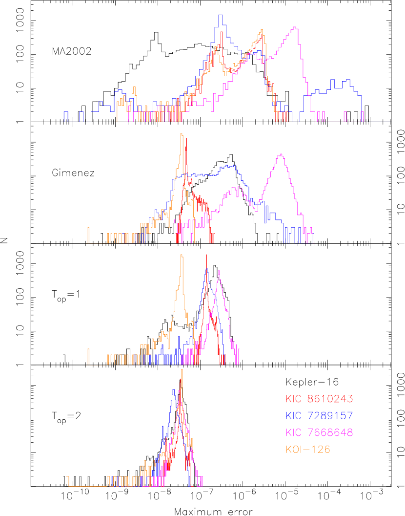
Figure 20: The statistics for the comparisons between model light curves generated using the MA2002 occultquad (top), the Giménez (2006a) routines (second from top), models with $T_{\rm op}=1$ (second from bottom), and models $T_{\rm op}=2$ (bottom). The histograms show the distribution of the maximum errors found for 5000 models of Kepler-16 (black lines), KIC 8610243 (red lines), KIC 7289157 (blue lines), KIC 7668648 (cyan lines), and KOI-126 (orange lines).

Figure 20 shows the distributions for the maximum differences. Over the five sources, occultquad gives the largest spreads in the maximum differences, where the maximum difference in many of the models can be as small as $10^{-10}$, or as large as $10^{-3}$. The sources KIC 7668648 and KIC 7289157 were the most problematic for occultquad, as there was a large number of models where the maximum difference was between $10^{-5}$ and $10^{-3}$. The Giménez routine gave the next largest spread of values, where the maximum error encountered was just over $10^{-5}$. As was the case with occultquad, the sources KIC 7668648 and KIC 7289157 caused the most difficulties. The set of models with $T_{\rm op}=1$ and $T_{\rm op}=2$ give the tightest ranges in the maximum error. When $T_{\rm op}=1$, the maximum error seen is $6\times 10^{-6}$ and when $T_{\rm op}=2$, the maximum error seen is just over $10^{-7}$, in agreement with the extensive tests performed above.

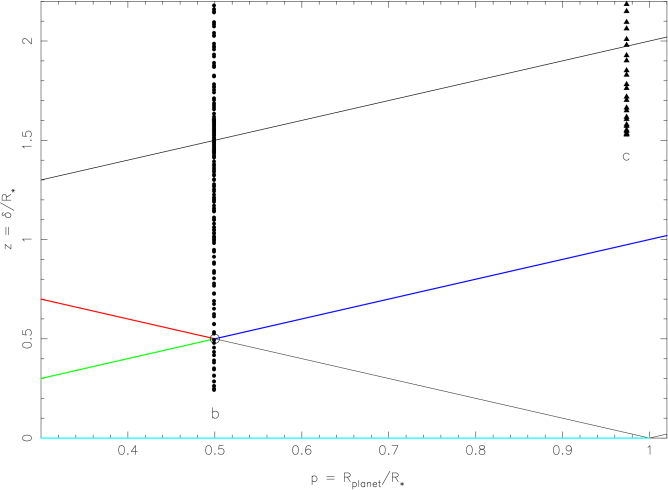
Figure 23: Left: The $(p,z)$ plane showing the various cases used to compute eclipse events in the MA2002 algorithm. The filled circles show the location of the points in the event labeled b in the upper right of Figure 22. The filled triangles show the location of the points in the event labeled as c in the upper right of Figure 22. In the case for event b, the ratio of radii is 0.49902, so the points pass very close to the intersections of several regions.

These simulations show that while occultquad generates lightcurves with small errors most of the time, there will be a non-negligible number of models where there is a large error somewhere. In addition, during the course of these simulations, we found a few cases where the differences between the models computed with the new method and models computed with occultquad were very large and systematic (i.e. not simply a “spike” in the difference curve). Figure 21 shows an example for KIC 7668648, where the differences between a model (computed with $T_{\rm op}=2$) and a model computed with occultquad approach one thousand parts per million. This particular model has $R_{1}=1.77666\,R_{\odot}$ and $R_{2}=0.88963\,R_{\odot}$, which gives $p=0.50073$. This value of $p$ is very close to $p=0.5$, which is where several regions intersect in the $(p,z)$ plane. Similarly, Figure 22 shows an example for KIC 7289157, where the differences between a model (computed with $T_{\rm op}=2$) and a model computed with occultquad are several hundred parts per million. Note that in both cases the differences between our models (with $T_{\rm op}=2$) and the Giménez models (with $N_{\rm terms}=300$) are smaller (in absolute value) than about 7 parts per million. This is shown in the middle panels of each figure. The upper panel of Figure 22 shows occultations of the third star by the second star (labeled a, b, and d) in KIC 7289157, and an occultation of the third star by the first star (labeled c). Interestingly, the differences between our method and occultquad of events a, b, and d shown in the lower right panel of Figure 22 are large, whereas the differences for event c are small. In Figure 23 we plot the locations of these events in the $(p,z)$ plane. For event b, the $p$ co-ordinate is 0.499012, and there are points that fall within occultquad regions 9, 3, and 2. In addition, the lines denoting regions 5 and 4 are crossed, and a few of the points come very close to the single point that is region 6. We noted earlier that regions 4 and 5 are lines in the plane and will never be reached in an actual calculation, so the boundaries are “fattened” inside the occultquad routine by multiplying various factors of $z+p$, $z-p$, and $1-p$ by constants equal to $10^{-4}$ or 1.0001, depending on the case. Thus it seems likely that for the light curve shown in Figure 22, incorrect regions in the $(p,z)$ plane were used for the occultation events a, b, and d. On the other hand, the eclipse event labeled c falls in the middle of region 2 far away from the boundaries of other regions (apart from region 1 where there is no overlap). As a result the light curve for this event computed by occultquad closely matches the light curve computed with $T_{\rm op}=2$.

It is less straightforward to directly compare our method to that of Pál (2012) since the subroutines provided by Pál are written in C, and ELC is written in FORTRAN. In order to make a few direct comparisons between the two methods, we used Josh Carter’s Photodynam code (Carter et al., 2011; Doyle et al., 2011), which is publicly available. Photodynam takes initial conditions in the form of orbital elements and integrates the Newtonian equations of motion to produce POS co-ordinates and velocities. When given POS positions and the radius of each body, it then computes the flux fractions using Pál’s subroutines (which use the quadratic limb darkening law). We computed the light curve of the example 5-body system introduced in Section 4.3 using both codes and took the difference between the two (a tolerance of $T_{\rm pan}=128$ was used for the light curve computed using our method). The results are shown in Figure 24. For the syzygy event involving five bodies, and for a primary eclipse involving two bodies, the maximum difference is on the order of $10^{-8}$. For a total secondary eclipse, the maximum difference is on the order of $10^{-7}$. The difference curves are not quite symmetric about zero, and we attribute this to small discrepancies in the positions of the bodies as a function of time, since ELC and Photodynam use different methods to solve the Newtonian equations of motion (the initial barycentric co-ordinates agree to better than $3\times 10^{-14}$ AU, and the initial POS co-ordinates, corrected for light travel time, agree to better than $5\times 10^{-9}$ AU).

When examining the differences between our method and that of Pál (2012), it is instructive to look at the difference curve made from our $T_{\rm pan}=128$ model and the model computed with occultquad within ELC. While occultquad cannot be used for true syzygy events, it works well close to the very start and the very end of the event near day 10, where the light curve is the superposition of several individual transits. For the total secondary eclipse, the difference curve between our method and Pál’s method (middle right panel in Figure 24) looks broadly similar to the difference curve between our method and occultquad (lower right panel in Figure 24). Pál (2012) noted similarities between terms in his expression for the flux fraction (his Equation 34 for the linear limb darkening law) and those of MA2002. Only one region (Region 8) is required in occultquad to compute the ingress and egress of the total eclipse, hence only one expression is used for the flux fraction. In this case, the difference curves look similar. On the other hand, several regions are required in occultquad to compute the primary eclipse, so several expressions are pieced together to produce the transit profile. In that case, the difference curves look rather dissimilar and completely different in scale.

We can compare the R-M curves computed with our method to those computed using the method of Giménez (2006b). For the first comparison we used KIC 7289157. The third star in this system (with $R=1.08\,R_{\odot}$), which is about as bright as the primary in the binary, is eclipsed by the primary and secondary stars at a variety of different impact parameters. Not knowing the orientation of the rotation axis of the third star, we assume $\Phi_{\rm rot}=90^{\circ}$ and $\Theta_{\rm rot}=0$. These angles would make the rotation axis of the star slightly misaligned with its orbital plane about the barycenter. Furthermore, we assume this star rotates 10 times faster than its orbital period of 243 days. Figure 25 shows five tertiary events in KIC 7289157, where either the primary passes in front of the third star (1/3 in the figure), or the secondary passes in front of the third star (2/3 in the figure). The impact parameters are given. The amplitudes of the R-M signal range from about 50 m s^-1 to about 250 m s^-1. Note the variety of shapes. The difference between the R-M curves computed with our method and those computed with the Giménez (2006b) method are shown as well. The largest differences in absolute value are about $10^{-2}{\rm m~{}s^{-1}}$ for the second and third events, and $\approx 100$ times smaller for the other three.

We also computed R-M curves for Kepler-16, specifically for a primary eclipse, for a planet transit of the primary, and for a (total) secondary eclipse. Figure 26 shows the light curves, the R-M curves, and the difference curves. The R-M effect for the primary star has an amplitude of $\approx 50~{}{\rm m~{}s^{-1}}$, and was observed by Winn et al. (2011). The R-M signal for the secondary star is much larger, but given that the secondary star is only a few percent as bright as the primary star, the R-M signal for the secondary is probably not observable. Note that the R-M signal is not defined during totality since the secondary is completely hidden by the primary. The differences in absolute value between the two methods for the primary star events are a few mm s^-1, which seems to be sufficiently small. For the total secondary eclipse, the absolute value differences are about 100 mm s^-1 near the onset of totality.

6 Worked Example: KOI-126

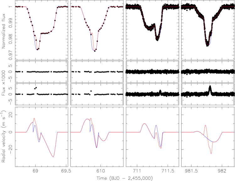
Figure 27: Top: The light curves of KOI-126 showing four syzygy events. The two panels on the left show the Kepler long-cadence data, and the other two panels show Kepler short cadence data. The red lines are the model computed with our new method, and the blue line shows the model computed using the Giménez (2006a) routine for the same model parameters. Middle: The O-C residuals computed for each model. Bottom: The R-M signal computed for each transit event using our new method (red line) and the Giménez (2006b) method (blue line).

Let us return to the system KOI-126 (KIC5897826), a low-mass, short-period binary ($P=1.74$ days) in eccentric 33.5 day orbit about a much larger $1.35M_{\odot}$ F-star star (Carter et al., 2011). The system has several distinct syzygies. We computed models for these syzygy events using both our new method and the Giménez (2006a) method, which will not work well for the syzygies. These models are shown in Figure 27. In all of the cases shown, our model, which accounts for the mutual overlap between the three bodies, provides a significantly better match to the observations. We also show in the figure the expected R-M effect signal, where the orbital motion of the F-star has been removed. The signals are complex and have a maximum velocity displacement on the order of 30 m s^-1, which may be detectable.

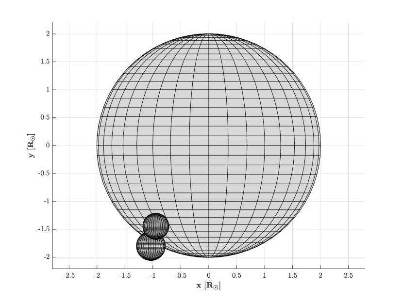
Figure 28: The POS view of the three bodies in KOI-126, during the syzygy event at day BJD 2455711.38. The axes are given in Solar radius for convenience. The configuration’s origin is the center of the back body, and the foreground binary is moving to the left

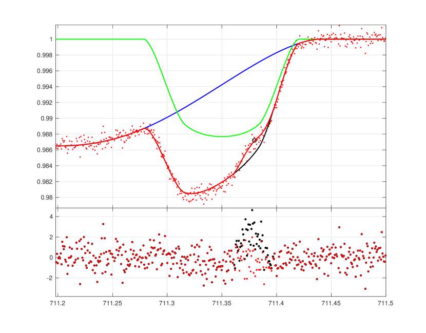
Figure 29: Modeling of a syzygy event in KOI-126, where the open circle marks the time corresponding to the configuration shown in Figure 28 and the example computation we presented in Section 6. The red dots show the normalized $Kepler$ short cadence data, where only a small part of the whole transit event is shown (the $x$-axis gives the time in days since BJD 2455000). The red line shows our model that accounts for mutual overlaps of the transiting stars; the blue line shows the expected light curve for the primary star transit of the third star; the green line shows the expected light curve for the secondary star transit of the third star; the black line is a simple combination of the two events, which would ignore overlaps between the primary and the secondary. The bottom panel shows the O-C residuals using the full model (red points) and the model that ignores overlaps (black points). The $\chi^{2}$ of the fit using the model that accounts for mutual overlaps improves from 976.1 to 849.3. As one might expect from the large feature in the residual near day $711.35$, the improvement in the fit is very significant.

To demonstrate the computation of the fractional flux we choose the time in the third syzygy event near BJD 2455711.38. Figure 28 shows the POS view of this event. We start this computation with the POS co-ordinates of the three bodies and their radii, provided in Table 3. In §6.1 we will show the vector stacks that are the bounding curves, denoted $Arc_{MN}$, for the visible and shadow paths of the three bodies, calculated as explained in §3. Note especially our description in §3 and in Appendix A of the process that allows us to generate the visible path. In §6.2 we will describe how the visible path is integrated and summed over these arcs using Equation (25). We will show in detail the calculation of the first and second integrals in this process. Figure 29 shows the resultant synthesized light curve superimposed on the $Kepler$ data with and without modeling the overlap. We note the significant reduction in the $\chi^{2}$ fit to the data by properly treating the syzygy.

6.1 The Boundary Paths

Table 3 lists the POS co-ordinates. They are arranged from the closest to the farthest along our line of sight. Note that in our co-ordinate system, positive z is toward the observer.

Following the method as outlined in §3, we first need to describe the visible region of each body, beginning with the front body, and iteratively determine the visible path for each body as we proceed along the line of sight. Each step in this process has two parts: updating the shadow path formed by all of the preceding bodies, then using that shadow path to determine the visible path of the current body. As described in §3, the visible path and the shadow path contain arcs that are stored in a vector stack. See specifically Equation (6) and Equation (22) for the notation. Since the front body is unobstructed, the bounding arc for it is the entire circumference as is the shadow that it casts.

$$\begin{aligned} VisiblePath(Body1)=\begin{bmatrix}\vspace{0.02in}1&1&0&360&360\end{bmatrix}\\ ShadowPath(Body1)=\begin{bmatrix}\vspace{0.02in}1&1&0&360&360\end{bmatrix}\end{aligned}$$ (39)

where the angles are given in degrees for ease of exposition.

Now consider the second body and its relationship to the shadow of the previous body. We see that the boundary of the second body intersects the shadow arc, hence the visible portion is described by two arcs (see §A.3, Equation A13):

$$\begin{aligned} VisiblePath(Body2)=\begin{bmatrix}\vspace{0.02in}2&1&210.87&90.103&300.97\\ \end{bmatrix}\\ \begin{bmatrix}\vspace{0.02in}2&2&115.52&280.81&396.33\\ \end{bmatrix}\\ \end{aligned}$$ (40)

The new shadow is also described by two arcs (§A.3), Equation (A14):

$$\begin{aligned} ShadowPath(Body2)=\begin{bmatrix}\vspace{0.02in}1&1&300.97&269.90&570.87\\ \end{bmatrix}\\ \begin{bmatrix}\vspace{0.02in}2&2&115.52&280.81&396.33\\ \end{bmatrix}\\ \end{aligned}$$ (41)

Now consider the third body and its relationship to the shadow of the previous bodies. Note that the first arc in the shadow is entirely contained within the current body (Body 3) and that the second arc is only partially contained within Body 3.

$$\begin{aligned} VisiblePath(Body3)=\begin{bmatrix}\vspace{0.02in}3&1&300.97&269.90&570.87\\ \end{bmatrix}\\ \begin{bmatrix}\vspace{0.02in}3&2&349.60&46.729&396.33\\ \end{bmatrix}\\ \begin{bmatrix}\vspace{0.02in}3&2&115.52&15.045&130.56\\ \end{bmatrix}\\ \begin{bmatrix}\vspace{0.02in}3&3&247.09&345.98&593.07\\ \end{bmatrix}\\ \end{aligned}$$ (42)

Although the shadow is not required for this example, it is given for completeness:

$$\begin{aligned} ShadowPath(Body3)=\begin{bmatrix}\vspace{0.02in}2&2&130.56&219.03&349.60\\ \end{bmatrix}\\ \begin{bmatrix}\vspace{0.02in}3&3&247.09&345.98&593.07\\ \end{bmatrix}\\ \end{aligned}$$ (43)

Note that since Body 1 lies within Body 3, the shadow no longer contains any Body 1 arcs.

The flux integral for each body may now be assembled using equations (5), (23), and (25), noting the value of the orientation given after Equation (25). Since the co-ordinate system used to describe the limb darkening law is centered on the body in question having radius 1, we must convert all of the arc descriptions to that coordinate system. That is why Equation (5) translates the origin of each body’s system to the origin of the body in question and scales the co-ordinates to radius 1 for that body. These flux integrals may now be evaluated in closed form or, if needed, numerically. If we normalize Equation (4) by the integral of the flux over the unobstructed disk, we obtain the flux fraction for the system at the given time.

6.2 Calculating the Fractional Flux

Continuing with the KOI-126 example, in §6.1 we constructed the bounding arcs for the visible portion of the three stars. Using these visible-path vector stacks, we will implement Equations (5)-(26) to compute the fractional flux of each body at the syzygy epoch BJD 2455711.38 (refer to Table 3). For simplicity we will use the linear limb darkening law for all stars, with a coefficient of $0.6$. Repeating Equations 12, 13 we have

$$I(\mu)/I_{0}=\bm{C}\bm{\cdot}\bm{\Psi}\text{~{}where~{}}{\bm{C}}=\big{[}(1-c_{1}),c_{1}\big{]}\text{~{}~{}and~{}~{}}\bm{\Psi}=\big{[}\bm{1},\mu\big{]}$$

Substituting the exterior anti-derivatives of the functions in the $\Psi$ vector from Table 1 into Equation (21) gives:

$$I_{\rm vis}=\bm{C}\bm{\cdot}\bigg{[}\oint\displaylimits_{\partial D_{\rm vis}}\frac{1}{2}\big{[}-y,x\big{]}\bm{\cdot}\big{[}x^{\prime},y^{\prime}]d\varphi,\,\,\oint\displaylimits_{\partial D_{\rm vis}}\frac{1-\mu^{3}}{3r^{2}}\big{[}-y,x\big{]}\bm{\cdot}\big{[}x^{\prime},y^{\prime}]d\varphi\bigg{]}$$ (44)

For each body, in turn, we will evaluate the line integrals in the $\Psi$ vector over the arcs described by that body’s visible-path stacks. For Body 1:

$$\begin{aligned} VisiblePath(Body1)=\begin{bmatrix}\vspace{0.02in}1&1&0&360&360\end{bmatrix}\text{~{}or in radians:~{}}\begin{bmatrix}\vspace{0.02in}1&1&0&2\pi&2\pi\end{bmatrix}\\ \end{aligned}$$ (45)

This is the front body, which is entirely visible, thus the flux fraction, ${\cal F}=1$. For Body 2:

$$\begin{aligned} VisiblePath(Body2)=\begin{bmatrix}\vspace{0.02in}2&1&210.87&90.103&300.97\end{bmatrix}\begin{bmatrix}\vspace{0.02in}2&2&115.52&280.81&396.33\end{bmatrix}\\ \text{~{}or in radians:~{}}VisiblePath(Body2)=\begin{bmatrix}\vspace{0.02in}2&1&3.6804&1.5726&5.253\end{bmatrix}\begin{bmatrix}\vspace{0.02in}2&2&2.0162&4.901&6.9172\end{bmatrix}\\ \end{aligned}$$ (46)

In this case, the boundary of the visible region is described by two arcs:

$$\begin{aligned} Arc_{MN}=\begin{bmatrix}\vspace{0.02in}2&1&210.87&90.103&300.97\end{bmatrix}\end{aligned}$$ (47)

where $N=2$ and $M=1$. The limits of integration are $\varphi_{0}=3.6804$ and $\varphi_{1}=5.253$. The parametric equations for this arc are given by Equation (5) and the derivatives by Equation (23).

$$\begin{aligned} &x_{1}=0.90058\cos(\varphi)+0.34217&y_{1}&=0.90058\sin(\varphi)+1.3645\\ &x_{1}^{\prime}=-0.90058\sin(\varphi)&y_{1}^{\prime}&=-0.90058\cos(\varphi)\end{aligned}$$ (48)

Now assemble the integral $j=1$ (constant function) and $i=1$ (arc $1$) in Equation (23) by substituting the expressions for $x_{1}$ and $y_{1}$

$$\begin{aligned} \Psi_{1,1}=\oint\displaylimits_{\varphi_{0}}^{\varphi_{1}}{\rm Orientation}\times\big{[}P_{1},Q_{1}\big{]}\bm{\cdot}\big{[}x^{\prime}_{1},y^{\prime}_{1}\big{]}d\varphi=\int\displaylimits_{\varphi_{0}}^{\varphi_{1}}(-1)\frac{1}{2}\big{[}-y_{1},x_{1}\big{]}\bm{\cdot}\big{[}x^{\prime}_{1},y^{\prime}_{1}\big{]}d\varphi=0.25893\end{aligned}$$ (49)

Since $M<N$, the orientation is $-1$. Next, assemble the integral $j=2$ (the $\mu$ function) and $i=1$ (arc 1) in Equation (23), by substituting the expressions for $x_{1}$ and $y_{1}$, and noting the definitions of $r$ and $\mu$:

$$\begin{aligned} \Psi_{2,1}=\oint\displaylimits_{\varphi_{0}}^{\varphi_{1}}{\rm Orientation}\times\big{[}P_{2},Q_{2}\big{]}\bm{\cdot}\big{[}x^{\prime}_{1},y^{\prime}_{1}\big{]}d\varphi=\int\displaylimits_{\varphi_{0}}^{\varphi_{1}}(-1)\frac{1-\mu^{3}}{3r^{2}}\big{[}-y_{1},x_{1}\big{]}\bm{\cdot}\big{[}x^{\prime}_{1},y^{\prime}_{1}\big{]}d\varphi=0.22757\end{aligned}$$ (50)

Since $M<N$, the orientation is $-1$. Moving on to the second arc:

$$\begin{aligned} Arc_{MN}=\begin{bmatrix}2&2&2.0162&4.901&6.9172\end{bmatrix}\end{aligned}$$ (51)

where $N=2$ and $M=2$. The limits of integration are $\varphi_{0}=2.0162$ and $\varphi_{1}=6.9172$. The parametric equations for this arc are given by Equation (5) and the derivatives are given by Equation (23).

$$\begin{aligned} &x_{1}=\cos(\varphi)&y_{1}&=\sin(\varphi)\\ &x_{1}^{\prime}=-\sin(\varphi)&y_{1}^{\prime}&=\cos(\varphi)\end{aligned}$$ (52)

Now assemble the integral $j=1$ (constant function) and $i=2$ (arc 2) in Equation (25) by substituting the expressions for $x_{1}$ and $y_{1}$:

$$\begin{aligned} \Psi_{1,2}=\oint\displaylimits_{\varphi_{0}}^{\varphi_{1}}{\rm Orientation}\times\big{[}P_{1},Q_{1}\big{]}\bm{\cdot}\big{[}x^{\prime}_{1},y^{\prime}_{1}\big{]}d\varphi=\int\displaylimits_{\varphi_{0}}^{\varphi_{1}}(+1)\frac{1}{2}\big{[}-y_{1},x_{1}\big{]}\bm{\cdot}\big{[}x^{\prime}_{1},y^{\prime}_{1}\big{]}d\varphi=0.4505\end{aligned}$$ (53)

Since $M=N$, the orientation is $+1$. Next, assemble the integrand $j=2$ (the $\mu$ function) and $i=2$ (arc 2) in Equation (25) by substituting the expressions for $x_{1}$ and $y_{1}$ and noting the definitions of $r$ and $\mu$:

$$\begin{aligned} \Psi_{2,2}=\oint\displaylimits_{\varphi_{0}}^{\varphi_{1}}{\rm Orientation}\times\big{[}P_{2},Q_{2}\big{]}\bm{\cdot}\big{[}x^{\prime}_{1},y^{\prime}_{1}\big{]}d\varphi=\int\displaylimits_{\varphi_{0}}^{\varphi_{1}}(+1)\frac{1-\mu^{3}}{3r^{2}}\big{[}-y_{1},x_{1}\big{]}\bm{\cdot}\big{[}x^{\prime}_{1},y^{\prime}_{1}\big{]}d\varphi=1.6337.\end{aligned}$$ (54)

Since $M=N$, the orientation is $+1$. Thus, Equation (25) results in

$$\begin{aligned} \Psi_{1}&=\Psi_{1,1}+\Psi_{1,2}=2.7094\text{~{}~{}and~{}~{}}\Psi_{2,1}+\Psi_{2,2}=1.8612\\ \Longrightarrow I_{\rm vis}&=\bm{C}\bm{\cdot}\big{[}2.7094,1.8612\big{]}=\big{[}1-0.6,0.6\big{]}\bm{\cdot}\big{[}2.7094,1.8612\big{]}=2.2005\end{aligned}$$ (55)

Following the computation for arc $2$ we can easily compute $I_{\rm total}$, which is the integral over the entire disk. The boundary consists of one arc: $\big{[}2~{}~{}2~{}~{}0~{}~{}2\pi~{}~{}2\pi\big{]}$:

$$\begin{aligned} I_{\rm total}&=\bm{C}\bm{\cdot}\big{[}3.1416,2.0944\big{]}=\big{[}1-0.6,0.6\big{]}\bm{\cdot}\big{[}3.1416,2.0944\big{]}=2.5133\end{aligned}$$ (56)

The flux fraction of Body 2 is then $2.2005/2.5133=0.87556$. Following a similar procedure, we can compute the flux fraction of the third star, which in this case is the bright F-star that dominates the total system light. As shown in Equation (42), the visible path of that star has $4$ arcs at this particular time, hence there are $8$ terms in the summation, along with a normalizing term. The final result is $F_{3}=0.98628$ (we omit the details for brevity).

7 Summary

We presented here an efficient method for computing the visible flux for each body during a multi-body eclipsing event for all commonly used limb darkening laws. The method can also calculate the R-M effect. Our approach follows the idea put forth by Pál (2012) to apply Green’s Theorem, thus transforming the 2D POS flux integral into a 1D integral over the visible boundary. We executed this idea through an iterative process which combines a fast method for describing the visible boundary of each body with a fast and accurate Gaussian integration scheme to compute the integrals.

We first provided the mathematical background for the method, then compare the results of its application to three other methods currently used, i.e.  Mandel & Agol (2002), Giménez (2006a), and Pál (2012). Finally, we explained in detail how to implement the technique with the help of several examples and a code which we made available. Specifically, we note that for the two body case, our method compares well in speed with that of Mandel & Agol (2002), and is faster than that of Giménez (2006a); the method does not have various distinct cases so it does not produce the occasional spikes and other numerical anomalies caused by crossing boundaries as is seen in the Mandel & Agol technique; the method uses a tolerance parameter, $T_{\rm op}$, which sets the computational error to the problem being worked. Most significantly, the method works for any number of eclipsing bodies, and using a multitude of limb darkening laws (including all of the commonly used ones). It can also compute the R-M effect for any of these limb darkening laws. This method can be extended to stars with differential rotation when using the quadratic limb darkening.

We note that in applying Green’s Theorem to solve the flux integral, we are not necessarily limited to using spherical bodies. For example, one might wish to compute the transits of an ellipsoidal body with any orientation.

Appendix A Constructing the Visible Boundary - a Worked Example

A.1 The Special Two Body Case

When constructing the bounding curves we employ four operations: we can intersect two different circles (the routine XCircle in the code); we can find the complement of an arc in a given circle (XComp in the code); we can intersect two arcs within a given circle (XSect); and we can intersect multiple arcs in a given circle (XSectAll). In the following sections we show how these routines are used to find the visible paths needed for the fractional flux computation.

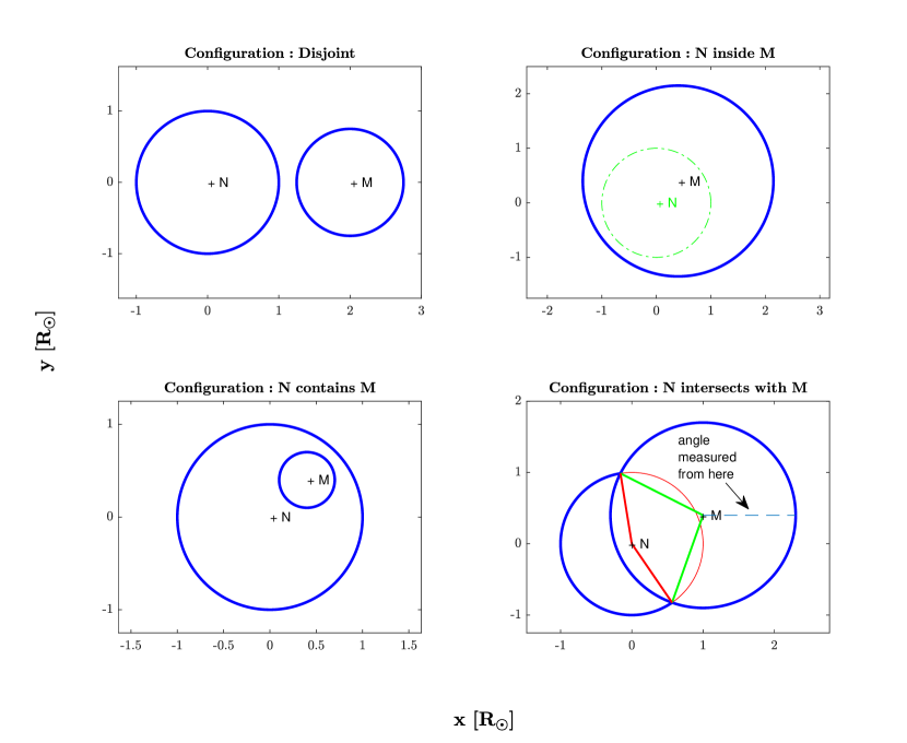
Figure 30: The four possible intersections of two circles used when starting the construction of a bounding arc (§3 and Appendix A.1). The body in the back (further from the observer) is always denoted $N$ and the body in the front (closer to the observer) is always denoted $M$. The upper Left panel shows the disjoint case with no arc intersection. The Upper right panel shows the case when the body in the back (labeled $N$) is completely covered by the body in the front (labeled $M$). The lower Left panel shows the case when the smaller body in the front ($M$) is completely within the boundary of the body in the back ($M$). The lower right panel shows the intersection case where the body in front ($M$) partially covers the body in the back ($N$). The visible part of the body in the back is described by these two arcs: $Arc_{NM}=\big{[}N~{}~{}M~{}~{}153.150~{}~{}97.301~{}~{}250.452\big{]}$ and $Arc_{NN}=\big{[}N~{}~{}N~{}~{}99.198~{}~{}205.205~{}~{}304.404\big{]}$, where the angles are measured in degrees.

If we have only two bodies to consider, where Body $M$ is closer to the observer and body $N$ is further from the observer, XCircle is the only one of the four routines mentioned above that we need to use. The operation XCircle has one of four possible outcomes, as shown in Figure 30: I. The two bodies are disjoint and do not intersect. II. Body $N$ is contained in Body $M$. III. Body $N$ contains body $M$. IV. There is partial overlap and the boundaries of each body intersect at two points. In the first three cases, the routine returns special flags to indicate which case was encountered. In the last case, the routine returns the two arcs that make up the visible path of Body $N$. It is important to select the correct arcs, since given two points on the circumference of a circle, one can draw two different arcs. The first arc can go from $\varphi_{0}$ to $\varphi_{1}$ (following the right-hand rule), and the second arc can go from $\varphi_{1}$ to $\varphi_{0}$. Which arc do we choose when constructing the visible path on Body $N$ For the arc centered on Body $M$, we want the arc that is closer to the center of Body $N$. Likewise, for the arc centered on Body $N$, we want the arc that is furthest from the center of body $M$. By considering the triangles formed by the two centers and each of the intersection points, and by using the Law of Cosines, we can ensure the correct arcs are chosen.

In the discussion below we explicitly give the appropriate visible arc(s) for the four possible outcomes of XCircle. For completeness, we also give the correspondng shadow paths for each case for situations where additional bodies need to be considered (the shadow paths are not required for the light curve computation, when ${\cal N}=2$).

I. The bodies are disjoint (top-left panel in Figure 30). Since there is no overlap between the two circles, the entire boundary of Body $N$ is visible. If one were to continue to the next stage where there is a third body in the back of these two bodies, the shadow boundary would simply be composed of the outer parts of each circle. Following the notation of Equation (6), the visible path and shadow path are written as:

$$\begin{aligned} Visible~{}path=\begin{bmatrix}\vspace{0.02in}N&N&0&360&360\end{bmatrix}\\ Shadow~{}path=\begin{bmatrix}\vspace{0.02in}N&N&0&360&360\end{bmatrix}\\ \begin{bmatrix}\vspace{0.02in}M&M&0&360&360\end{bmatrix}\end{aligned}$$ (A1)

where all angles are given in degrees, for the reader’s convenience. In this particular case, $N=2$ and $M=1$ following the convention of front-to-back order.

II. Body $N$ is contained in Body $M$ (i.e. body $N$ is totally eclipsed by body $M$, top-right panel in Figure 30). In this case, since Body $N$ is completely obstructed by Body $M$, there is no visible path on Body $N$. Therefore, the arc is of zero length. If one were to continue to an additional third body that is behind these two bodies, one could see that the shadow cast by the two bodies $N$ and $M$ would be bounded by the outer part of body $M$. Thus, following the notation of Equation (6), the visible path and the shadow path are written as:

$$\begin{aligned} Visible~{}path=\begin{bmatrix}\vspace{0.02in}N&N&0&0&0\end{bmatrix}\\ Shadow~{}path=\begin{bmatrix}\vspace{0.02in}M&M&0&360&360\end{bmatrix}\end{aligned}$$ (A2)

III. Body $N$ contains Body $M$ (i.e. body $M$ is transiting body $N$, bottom-left panel in Figure 30), Here, the visible path on Body $N$ is an annulus, made of arcs that are two full circles. One of the circles is centered on Body $M$ and the other circle is centered on Body $N$. Since one body is contained within the other, the shadow path is simply the boundary of the larger of the two bodies, Body $N$. Hence, the visible path and the shadow path are written below in the notation of Equation (6) as:

$$\begin{aligned} Visible~{}path=\begin{bmatrix}\vspace{0.02in}N&M&0&360&360\\ \end{bmatrix}\\ \begin{bmatrix}\vspace{0.02in}N&N&0&360&360\end{bmatrix}&\\ Shadow~{}path=\begin{bmatrix}\vspace{0.02in}N&N&0&360&360\end{bmatrix}\end{aligned}$$ (A3)

IV. The boundary of Body $N$ and the boundary of Body $M$ intersect (bottom-right panel in Figure 30). In this case, the visible path on Body $N$ will have two arcs, one centered on Body $M$, and the other centered on Body $N$. These arcs are output by the XCircle routine. In a similar manner, the boundary of the shadow cast by these two bodies will consist of two arcs. The first arc, centered on Body $M$, will be the complement of the arc (centered on Body $M$) that appeared in the visible path on Body $N$. The second arc, centered on Body $N$, will be the same arc centered on Body $N$ that was in the visible path. In the notation of Equation (6), the visible path and shadow path are therefore written as:

$$\begin{aligned} Visible~{}path=\begin{bmatrix}\vspace{0.02in}N&M&\varphi_{0}&\Delta\varphi&\varphi_{1}\end{bmatrix}\\ \begin{bmatrix}\vspace{0.02in}N&N&\psi_{0}&\Delta\psi&\psi_{1}\end{bmatrix}\\ Shadow~{}path=\begin{bmatrix}\vspace{0.02in}M&M&\rm{complement}(\varphi_{0},\varphi_{1})\end{bmatrix}\\ \begin{bmatrix}\vspace{0.02in}N&N&\psi_{0}&\Delta\psi&\psi_{1}\end{bmatrix}\end{aligned}$$ (A4)

The “$\rm{complement}(\varphi_{0},\varphi_{1})$” in Equation (A4) is the complementary arc to $(\varphi_{0},\varphi_{1})$, and is obtained with the routine XComp in the code:

$$\begin{aligned} {\tt XComp}\bigg{(}\begin{bmatrix}\vspace{0.02in}N&M&\varphi_{0}&\Delta\varphi&\varphi_{1}\end{bmatrix}\bigg{)}=\begin{bmatrix}\vspace{0.02in}N&M&(\varphi_{1}-2\pi)&(2\pi-\Delta\varphi)&\varphi_{0}\end{bmatrix}\quad\varphi_{1}\geq 2\pi\\ \begin{bmatrix}\vspace{0.02in}N&M&\varphi_{1}&(2\pi-\Delta\varphi)&(2\pi+\varphi_{0})\end{bmatrix}\quad\varphi_{1}<2\pi\\ \end{aligned}$$ (A5)

A.2 The Case of Three or More Bodies

When there are three or more bodies, we can find the visible path on the third star (which is behind the other two) as follows. The shadow path of the first two bodies (which are closer to the observer) needs to be found as outlined above. That shadow path can be the outer boundary of either star (in the case of an occultation or transit), it can be the outer boundaries of both stars (in the case of no overlap), or it can resemble the outside of a“dumbell” (in the case of partial overlap). This shadow could cover parts of the third star. Therefore, the visible path on the third star (the one in the back) could consist of arcs on its own boundary and arcs from the shadow path of the first two stars. To do that, we use XCircle on Body 1 and Body 3 (the ordering that the subroutine uses is front, back), and also on Body 2 and Body 3. This results in two arcs on the perimeter of Body 3 that are potentially visible. These arcs could overlap, and we want to find their intersection. In addition, there might be arcs on the perimeter of Body 1 and on the perimeter of Body 2 that are potentially visible, and these arcs may overlap with arcs in the shadow path of the first two bodies. As before, we need to find their intersections. The routines XSect and XSectAll are used to find those.

If there is a fourth star, the shadow path of the three stars is required. The shadow path of the three bodies is formed by taking the union of the shadow path formed by the two front bodies with the visible path of the third body and then removing the extraneous interior arcs. This is done as follows: for each of the front bodies, we look at that body’s contribution to the visible path on the back body, we find the complimentary arcs to that contribution, and intersect them (using the routines XSect and XSectAll) with the arcs in the shadow path contributed by that front body. Finally, we add all of the visible arcs on the perimeter of the back body.

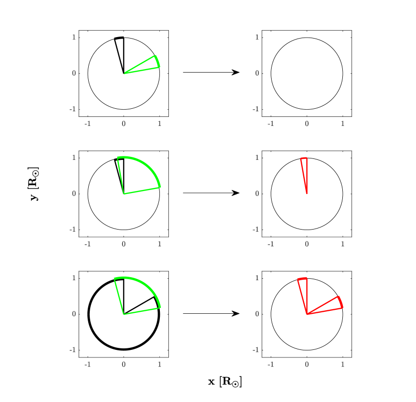
Figure 31: The three possibilities of intersecting two arcs, as demonstrated in §3 and Appendix A. The panels on the left show the two arcs to be intersected, and the panels on the right show the resulting arc. The two arcs in the top panels are disjoint, so the intersection is empty (Equation A6). The arcs in the middle panels intersect so that only a part of the smaller arc is preserved (Equation A7). The two arcs in the bottom panels intersect into two different, disjoint, arcs (Equation A8). In the code, this is done with the XSect routine.

In the following section we present an example of a system with four overlapping bodies, and explain step-by-step how to find the visible paths and the shadow boundaries. But first we show below how the routines XSect and XSectAll work. Consider the intersection of bounding arcs for a given disk. The simplest case is the intersection of two arcs (XSect). There are three possibilities, as shown by the following example (see Figure 31):

$$\begin{aligned} \text{No Overlap:}\begin{bmatrix}\vspace{0.02in}N&M&10&20&30\end{bmatrix}\cap\begin{bmatrix}\vspace{0.02in}N&M&90&15&105\end{bmatrix}\Longrightarrow~{}Empty\end{aligned}$$ (A6)

$$\begin{aligned} \text{Overlap (1 arc)}=\begin{bmatrix}\vspace{0.02in}N&M&10&90&100\end{bmatrix}\cap\begin{bmatrix}\vspace{0.02in}N&M&90&15&105\end{bmatrix}\Longrightarrow\begin{bmatrix}\vspace{0.02in}N&M&90&10&100\end{bmatrix}\end{aligned}$$ (A7)

$$\begin{aligned} \text{Overlap (2 arcs)}=\begin{bmatrix}\vspace{0.02in}N&M&10&95&105\end{bmatrix}\cap\begin{bmatrix}\vspace{0.02in}N&M&90&300&390\end{bmatrix}\Longrightarrow\begin{bmatrix}\vspace{0.02in}N&M&90&15&105\end{bmatrix}\\ \begin{bmatrix}\vspace{0.02in}N&M&10&20&30\end{bmatrix}\\ \end{aligned}$$ (A8)

If there are more than two arcs to be intersected, then we proceed iteratively, starting with the intersection of the first two, and intersecting the remaining arcs, in turn, with the intersection of the previous arcs (see the XSectAll routine). However, if at some step, the intersection, XSect, yields two arcs, the process bifurcates, as in Equation (A8). Those 2 arcs must be intersected individually with the remaining arcs. For example, consider the following three arcs:

$$\begin{aligned} \begin{bmatrix}\vspace{0.02in}N&M&10&95&105\end{bmatrix}\\ \begin{bmatrix}\vspace{0.02in}N&M&90&300&390\end{bmatrix}\\ \begin{bmatrix}\vspace{0.02in}N&M&25&70&95\end{bmatrix}\end{aligned}$$ (A9)

Intersect the first two:

$$\begin{aligned} \begin{bmatrix}\vspace{0.02in}N&M&10&95&105\end{bmatrix}\cap\begin{bmatrix}\vspace{0.02in}N&M&90&300&390\end{bmatrix}\Longrightarrow\begin{bmatrix}\vspace{0.02in}N&M&90&15&105\end{bmatrix}\\ \begin{bmatrix}\vspace{0.02in}N&M&10&20&30\end{bmatrix}\\ \end{aligned}$$ (A10)

Bifurcation yields two intersections, each with the remaining arc $\big{[}N~{}M~{}25~{}70~{}95\big{]}$:

$$\begin{aligned} \begin{bmatrix}\vspace{0.02in}N&M&90&15&105\end{bmatrix}\cap\begin{bmatrix}\vspace{0.02in}N&M&25&70&95\end{bmatrix}\Longrightarrow\begin{bmatrix}\vspace{0.02in}N&M&90&15&105\end{bmatrix}\\ \end{aligned}$$ (A11)

and

$$\begin{aligned} \begin{bmatrix}\vspace{0.02in}N&M&10&20&30\end{bmatrix}\cap\begin{bmatrix}\vspace{0.02in}N&M&25&70&95\end{bmatrix}\Longrightarrow\begin{bmatrix}\vspace{0.02in}N&M&25&5&30\end{bmatrix}\\ \end{aligned}$$ (A12)

Thus, the result of intersecting the three arcs in (A9) is two disjoint arcs (A11) and (A12).

We are now ready to present a worked example with four overlapping bodies

A.3 Worked Example: a Four Body System

To fully understand the details of this process, consider the following $4$-body illustrative example based on the plane-of-the-sky co-ordinates given in Table 4, corresponding to the 4-body crossing event shown in Figure 32.

We describe the boundary of the visible path of a particular body, say Body 3, as the stack of arcs denoted, for clarity, by $VisiblePath(Body3)$. In the code, this stack is held in the variable Path. Similarly, the variable $ShadowPath(Body3)$ refers to the shadow formed at the stage where Body 3 is the back body. In the code, this stack is held in the variable Bdr. Both Path and Bdr are assigned by the function IntegrationPaths. We occasionally refer to specific arcs. In those instances, we use the notation $(Body3,Arc2)$ referring to the second arc in the stack, centered on Body 3.

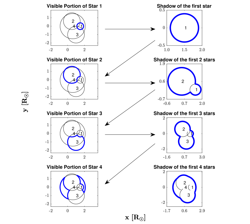
Figure 33: Construction of the Bounding Curve in the 4 body example given in §A.3 for the configuration shown in Figure 32. The panels on the left show the progression of the visible path of arcs, and those on the right show the shadow path of arcs resulting from each previous visible path. Both the visible path and the shadow path arcs are described as vector stacks in Equations (A13) - (A25). The arrows indicate the progression of the process where each visible path yields the shadow path which, in turn, is used to generate the next visible path. The process ends on the visible path of Star 4, but we show the resulting shadow path of Star 4 for completion.

To initialize the process, set $VisiblePath(Body1)$ and $ShadowPath(Body1)$ to the boundary of Body 1. This is shown in the upper two panels in Figure 33. The visible path and the shadow path are:

$$\begin{aligned} Visible\-Path(Body1)=\begin{bmatrix}\vspace{0.02in}1&1&0&360&360\end{bmatrix}\\ ShadowPath(Body1)=\begin{bmatrix}\vspace{0.02in}1&1&0&360&360\end{bmatrix}\end{aligned}$$ (A13)

where, again, all angles are given in degrees, for the reader’s convenience.

Now consider Body 2 and the shadow of Body 1 (see Figure 33). Using XCircle(Body1,Body2), two arcs are produced, which describe the visible portion of Body 2:

$$\begin{aligned} VisiblePath(Body2)=\begin{bmatrix}\vspace{0.02in}2&1&92.910&112.25&205.16\end{bmatrix}\\ \begin{bmatrix}\vspace{0.02in}2&2&348.43&321.21&669.64\end{bmatrix}\\ \end{aligned}$$ (A14)

The first arc is centered on Body 1 and the second arc is centered on Body2. We now compute the combined shadow of Body 1 and Body 2. Note that this requires the complement of the first arc, together with the second arc.

$$\begin{aligned} ShadowPath(Body2)=\begin{bmatrix}\vspace{0.02in}1&1&205.16&247.75&452.91\end{bmatrix}\\ \begin{bmatrix}\vspace{0.02in}2&2&348.43&321.21&669.64\end{bmatrix}\\ \end{aligned}$$ (A15)

Now consider Body 3. Here, for the first time, we see the complication of the general case (see Figure 33). We begin with the first arc of the shadow. The arc is centered on Body 1, so we use XCircle to find the two arcs detailing the portion of Body 3 that is not occluded by Body 1:

$$\begin{aligned} {\tt XCircle}(Body1,Body3)=\begin{bmatrix}\vspace{0.02in}3&1&180.72&125.43&306.15\end{bmatrix}\\ \begin{bmatrix}\vspace{0.02in}3&3&84.259&318.35&402.61\end{bmatrix}\\ \end{aligned}$$ (A16)

Note that the resulting arc, centered on Body 1, has a smaller starting angle than the shadow arc $(Body2,Arc1)$, while the shadow arc $(Body2,Arc1)$ has a larger ending angle than the arc from XCircle. Thus we must take the intersection of these arcs to obtain the visible arc $(Body3,Arc1)$. A similar intersection is required for Body 2:

$$\begin{aligned} {\tt XCircle}(Body2,Body3)=\begin{bmatrix}\vspace{0.02in}3&2&254.3&66.109&320.41\end{bmatrix}\\ \begin{bmatrix}\vspace{0.02in}3&3&140.41&293.89&434.3\end{bmatrix}\\ \end{aligned}$$ (A17)

Finally, for Body 3, the two arcs centered on Body 3 produced by XCircle must also be intersected, resulting in the following description of the boundary of Body 3:

$$\begin{aligned} VisiblePath(Body3)=\begin{bmatrix}\vspace{0.02in}3&1&205.16&100.99&306.15\end{bmatrix}\\ \begin{bmatrix}\vspace{0.02in}3&2&254.30&55.340&309.64\end{bmatrix}\\ \begin{bmatrix}\vspace{0.02in}3&3&140.41&262.20&402.61\end{bmatrix}\\ \end{aligned}$$ (A18)

Given $VisiblePath(Body3)$, we intersect the complement of the paths centered at Body 1 with those from the shadow centered at Body 1, do so for Body 2, and add in the Body 3 paths. This results in updating the shadow to that of Body 1, Body 2, and Body 3.

$$\begin{aligned} ShadowPath(Body3)=\begin{bmatrix}\vspace{0.02in}1&1&306.15&146.76&452.91\end{bmatrix}\\ \begin{bmatrix}\vspace{0.02in}2&2&348.43&265.87&614.30\end{bmatrix}\\ \begin{bmatrix}\vspace{0.02in}3&3&140.41&262.20&402.61\end{bmatrix}\\ \end{aligned}$$ (A19)

We now repeat the process to get the visible portion of Body 4. The first arc in $ShadowPath(Body3)$ is centered at Body 1. We, therefore, use XCircle to compute the arcs between Body 1 and Body 4.

$$\begin{aligned} {\tt XCircle}(Body1,Body4)=\begin{bmatrix}\vspace{0.02in}4&1&0&360&360\end{bmatrix}\\ \begin{bmatrix}\vspace{0.02in}4&4&0&360&360\end{bmatrix}\\ \end{aligned}$$ (A20)

Note that Body 1 is contained in Body 4, but we still get two arcs, $\big{[}4~{}1~{}0~{}360~{}360\big{]}$, and $\big{[}4~{}4~{}0~{}360~{}360\big{]}$. The first must be intersected with the shadow arc $(Body3,Arc1)$, giving $\big{[}4~{}1~{}306.15~{}146.76~{}452.91\big{]}$, and the second must be collected for intersection with all of the other $\big{[}4~{}4~{}x~{}x~{}x\big{]}$ arcs obtained during this step. Continuing the process of generating arcs, Body 2 and Body 3 are present in the shadow, which prompts the use of XCircle to compute the arcs between Body 4 and Body 2, and between Body 4 and Body 3.

$$\begin{aligned} {\tt XCircle}(Body2,Body4)=\begin{bmatrix}\vspace{0.02in}4&2&143.13&272.66&415.79\end{bmatrix}\\ \begin{bmatrix}\vspace{0.02in}4&4&126.87&305.18&432.05\end{bmatrix}\\ \end{aligned}$$ (A21)

$$\begin{aligned} {\tt XCircle}(Body3,Body4)=\begin{bmatrix}\vspace{0.02in}4&3&19.407&184.79&204.20\end{bmatrix}\\ \begin{bmatrix}\vspace{0.02in}4&4&333.57&276.47&610.04\end{bmatrix}\\ \end{aligned}$$ (A22)

As before, we intersect the visible arc $(Body4,Arc1)$ with the shadow arc $(Body1,Arc1)$. The next intersection of the visible arc $(Body4,Arc2)$ and shadow arc $(Body2,Arc2)$ brings a new complication. The intersection has two components:

$$\begin{aligned} \begin{bmatrix}\vspace{0.02in}4&2&348.43&67.362&415.79\end{bmatrix}\\ \begin{bmatrix}\vspace{0.02in}4&2&143.13&111.17&254.30\end{bmatrix}\\ \end{aligned}$$ (A23)

Likewise, the intersection of visible arc $(Body4,Arc3)$ and the shadow arc $(Body3,Arc3)$ has two components. The Visible Path is then given by:

$$\begin{aligned} VisiblePath(Body4)=\begin{bmatrix}\vspace{0.02in}4&1&306.15&146.76&452.91\end{bmatrix}\\ \begin{bmatrix}\vspace{0.02in}4&2&348.43&67.362&415.79\end{bmatrix}\\ \begin{bmatrix}\vspace{0.02in}4&2&143.13&111.17&254.30\end{bmatrix}\\ \begin{bmatrix}\vspace{0.02in}4&3&140.41&63.788&204.20\end{bmatrix}\\ \begin{bmatrix}\vspace{0.02in}4&3&19.407&23.204&42.611\end{bmatrix}\\ \begin{bmatrix}\vspace{0.02in}4&4&333.57&98.488&432.05\end{bmatrix}\\ \begin{bmatrix}\vspace{0.02in}4&4&126.87&123.17&250.04\end{bmatrix}\\ \end{aligned}$$ (A24)

Even though the shadow boundary is not required, it is given by:

$$\begin{aligned} ShadowPath(Body4)=\begin{bmatrix}\vspace{0.02in}2&2&55.795&87.336&143.13\end{bmatrix}\\ \begin{bmatrix}\vspace{0.02in}3&3&204.20&175.21&379.41\end{bmatrix}\\ \begin{bmatrix}\vspace{0.02in}4&4&333.57&98.488&432.05\end{bmatrix}\\ \begin{bmatrix}\vspace{0.02in}4&4&126.87&123.17&250.04\end{bmatrix}\\ \end{aligned}$$ (A25)

Note, for this particular example, Body 1 is completely contained within Body 4. The complement of the first arc in ${\tt XCircle}(Body1,Body4)$ is empty, and therefore does not contribute to $ShadowPath(Body4)$ from the first body.

We provide a FORTRAN code to both compute and plot the arcs on the visible path and shadow path boundaries for ${\cal N}$ bodies when given their radii, the POS co-ordinates of their centers, and their ordering in terms of their distance from the observer. In addition, we provide a Matlab code to produce this example.

Appendix B Exterior Derivatives

Every term in the limb darkening laws is of the form $f=f(r^{2})$, a continuous function on the unit disk. Since the 2-form $f(x,y)dxdy$ is a closed form on the unit disk, Poincaré’s Lemma asserts that there exists a 1-form $P(x,y)dx+Q(x,y)dy$ such that

$$d\wedge\big{[}P,Q\big{]}=\frac{\partial Q}{\partial x}-\frac{\partial P}{\partial y}=f(x,y)$$ (B1)

Try $P(x,y)=-yF(r^{2}),~{}~{}Q(x,y)=xF(r^{2})$ for some smooth function $F$ on the unit disk. Then

$$\begin{aligned} &\frac{\partial Q}{\partial x}-\frac{\partial P}{\partial y}=F(r^{2})+2x^{2}\frac{dF(r^{2})}{dr^{2}}+F(r^{2})+2y^{2}\frac{dF(r^{2})}{dr^{2}}\\ &\rm{or}\\ &2F(r^{2})+2r^{2}\frac{dF(r^{2})}{dr^{2}}=f(r^{2})\\ &{\rm or}\\ &\frac{2d\big{(}r^{2}F(r^{2})\big{)}}{dr^{2}}=f(r^{2})\end{aligned}$$ (B2)

integrating $f=f(z)$ with respect to $z$ where $z=r^{2}$, from $0$ to $r^{2}$, gives

$$\begin{aligned} 2r^{2}F(r^{2})=\int\displaylimits_{0}^{r^{2}}f(z)dz,\text{ hence}\\ F(r^{2})=\frac{{\int}\displaylimits_{0}^{r^{2}}f(z)dz}{2r^{2}}\end{aligned}$$ (B3)

and $P=-yF(r^{2}),~{}~{}Q=xF(r^{2})$ is the 1-form, the exterior derivative of which is $f(r^{2})$.

In the case of the R-M effect, all of the terms in Equation (26) (Equation 1 in Giménez 2006b) using any of the limb darkening laws have the 2-form $g=xf(r^{2})$ or $h=yf(r^{2})$ on the unit disk. Try

$$\begin{aligned} &P_{1}(x,y)=0&Q_{1}(x,y)&=G(r^{2})\\ &P_{2}(x,y)=G(r^{2})&Q_{2}(x,y)&=0\\ \end{aligned}$$ (B4)

Evaluating the partial derivatives for the first case only (the second case is very similar) yields:

$$\begin{aligned} &\frac{\partial P_{1}}{\partial y}=0\\ &\frac{\partial Q_{1}}{\partial x}=\frac{dG(r^{2})}{dr^{2}}(2x)=2x\frac{dG(r^{2})}{dr^{2}}=g(x,y)=xf(r^{2})\\ &{\rm or}~{}\frac{dG(r^{2})}{dr^{2}}=\frac{1}{2}f(r^{2})\\ \end{aligned}$$

which we then integrate:

$$\begin{aligned} &G(r^{2})=\frac{1}{2}\int\displaylimits_{0}^{r^{2}}f(z)dz\\ \end{aligned}$$

Hence

$$\begin{aligned} &d\wedge\big{[}0,G(r^{2})\big{]}=xf(r^{2})~{}\rm{and}\\ &d\wedge\big{[}-G(r^{2}),0\big{]}=yf(r^{2})\\ \end{aligned}$$

In summary,

$$\begin{aligned} G(r^{2})=\frac{1}{2}\int\displaylimits_{0}^{r^{2}}f(z)dz\\ \end{aligned}$$ (B5)

where $f=f(r^{2})$ is a continuous function on the unit disk. Then,

$$\begin{aligned} &d\wedge\bigg{[}-y\frac{G(r^{2})}{r^{2}},x\frac{G(r^{2})}{r^{2}}\bigg{]}=f(r^{2})\\ &d\wedge\bigg{[}0,G(r^{2})\bigg{]}=xf(r^{2})\\ &d\wedge\bigg{[}-G(r^{2}),0\bigg{]}=yf(r^{2})\\ \end{aligned}$$ (B6)

We note, again, that Equations (B6) explicitly gives the 1-forms $[P,Q]$ for the flux calculation for any limb darkening given by

$$\begin{aligned} I(\mu)/I_{0}=f(r^{2})=f(1-\mu^{2})\end{aligned}$$

(where $f$ is a continuous function on the disk $D$), and for the 1-forms $[P,Q]$ for the R-M effect based on that limb darkening. The specific form of the integral $G$ (Equation B5) will determine if $[P,Q]$ can be expressed in closed form, by a special function, or will require numerical evaluation.

Consider two special cases, $\mu^{p}$, and, $\mu\log(\mu)$.

$$\begin{aligned} &\rm{Let}~{}~{}f(r^{2})=\big{(}1-r^{2}\big{)}^{\text@frac{p}{2}}=\mu^{p}~{}~{}~{}(p\not=-2)\\ &G_{\rm pow}(r^{2})=\frac{1}{2}\int\displaylimits_{0}^{r^{2}}(1-z)^{\frac{p}{2}}dz\\ &{\rm if}~{}w=1-z,~{}~{}dw=-dz\\ &G_{\rm pow}(r^{2})=\frac{1}{2}\int\displaylimits_{1-r^{2}}^{1}w^{\frac{p}{2}}dw=\frac{1}{2}\frac{w^{\text@frac{p}{2}+1}}{(\frac{p}{2}+1)}\bigg{|}_{1-r^{2}}^{1}=\frac{1}{p+2}\bigg{[}1-\big{(}1-r^{2}\big{)}^{\text@frac{p+2}{2}}\bigg{]}\\ &~{}~{}~{}~{}~{}~{}~{}~{}~{}~{}~{}~{}=\frac{1}{p+2}\big{[}1-\mu^{p+2}\big{]}~{}~{}~{}(p\not=-2)\\ &\\ &\rm{Let}~{}~{}f(r^{2})=\sqrt{1-r^{2}}\log\big{(}\sqrt{1-r^{2}}\big{)}=\mu\log\mu\\ &G_{\rm log}(r^{2})=-\frac{1}{9}-\frac{\big{(}1-r^{2}\big{)}^{\text@frac{3}{2}}}{3}\bigg{[}\log\big{(}\sqrt{1-r^{2}}\big{)}-\frac{1}{3}\bigg{]}\\ \end{aligned}$$ (B7)

From the closed form expressions for $G$, we obtain closed form expressions for all of the 1-forms needed to efficiently apply Green’s Theorem to the computation of the flux fraction and the R-M effect (Equations 13-17). In Appendix C we extend this analysis to the R-M effect with differential stellar rotation. Note that Equation (B7) provides the closed form of the integral $G$ (Equation B5) needed to extend the computation of the flux fraction and the R-M effect to the power-2 law (Hestroffer, 1997; Maxted, 2018).

Appendix C Rossiter-McLaughlin Effect with Differential Stellar Rotation

For a star with differential rotation, the latitude variation in angular velocity will be modeled by the simple solar approximation

$$\omega=\omega_{e}\big{[}1-\varepsilon\cos^{2}(\varphi)\big{]}$$ (C1)

where $\omega_{e}$ is the equatorial angular velocity, $\varepsilon=\big{(}\omega_{e}-\omega_{\rm{pole}}\big{)}/\omega_{e}$, and $\varphi$ is the co-latitude with respect to the axis of rotation. From §4, the R-M effect is the product of a limb darkening law and the radial rotational velocity function. For this exposition, the quadratic law will be used. Thus, the integrand $F$ over the unit disk is given by

$$\begin{aligned} &F(x,y)=\big{[}1-c_{1}(1-\mu)-c_{2}(1-\mu)^{2}\big{]}\big{[}Ax+By\big{]}\omega\\ &\rm{or}\\ &F(x,y)=\big{[}1-(c_{1}+c_{2})+(c_{1}+2c_{2})\mu-c_{2}\mu^{2}\big{]}\big{[}Ax+By\big{]}\omega\\ \\ \end{aligned}$$ (C2)

where $A$ and $B$ are defined in Equation (31). The dynamical co-ordinates $(x,y,z)$ for the axis of rotation, $\Psi$, are given by

$$\begin{aligned} &\Psi=\big{[}-B,A,\cos(\Phi_{\rm rot})\big{]}~{}~{}\rm{and}\\ &\cos(\varphi)=\Psi\bm{\cdot}[x,y,\mu],~{}\rm{or}\\ &\cos(\varphi)=-Bx+Ay+\mu\cos(\Phi_{\rm rot})\\ &\Longrightarrow\omega=\omega_{e}\bigg{[}1-\varepsilon\bigg{(}-Bx+Ay+\mu\cos(\Phi_{\rm rot})\bigg{)}^{2}\bigg{]}\end{aligned}$$ (C3)

To compute the exterior anti-derivative of $F$, as in the previous cases of the computation of the flux fraction and the R-M effect, we will find the exterior anti-derivative for each simple term, compute the path integrals, apply the coefficients, and sum them up. The problem then becomes one of detailed bookkeeping.

For the product of the quadratic law and the rotational radial velocity field, the simple terms are

$$\begin{aligned} \big{[}x,x\mu,x\mu^{2},y,y\mu,y\mu^{2}\big{]}\end{aligned}$$

and for the latitude effect, they are

$$\begin{aligned} \big{[}1,x^{2},y^{2},\mu^{2},xy,x\mu,y\mu\big{]}\end{aligned}$$ (C4)

The product of these terms forms a $7\times 6$ array, $\rm{Terms_{i,j}}$, shown in Table 5, with a corresponding $7\times 6$ array of coefficients:

$$\rm{Coeff_{i,j}}=D_{i}E_{j}$$ (C5)

where the coefficients of the simple terms of the quadratic law and the rotational radial velocity field are given by

$$\begin{aligned} &\alpha=c_{1}+c_{2},~{}\beta=c_{1}+2c_{2}\\ &E=\big{[}A(1-\alpha),A\beta,-c_{2}A,B(1-\alpha),B\beta,-c_{2}B\big{]}\\ \end{aligned}$$ (C6)

and the coefficients of the simple terms of the Latitude effect are given by

$$\begin{aligned} &D_{1}=1\\ &D_{2}=-eB^{2}\\ &D_{3}=-eA^{2}\\ &D_{4}=-e\cos^{2}(\Phi_{\rm rot})\\ &D_{5}=2eAB\\ &D_{6}=2eB\cos(\Phi_{\rm rot})\\ &D_{7}=-2eA\cos(\Phi_{\rm rot})\\ \end{aligned}$$ (C7)

Thus,

$$\begin{aligned} F(x,y)=\omega\sum_{i\&j}\rm{Coeff_{ij}}\cdot{\rm Terms_{ij}}\end{aligned}$$ (C8)

Table 6 has the 1-forms for all of the simple terms in ${\rm Terms_{ij}}$ contained in Equation C8. Note that in the case of no latitude variation, the vector $D$ consists of just the first term, $D_{1}$, which then simplifies the coefficient matrix and Equation (C8).

Appendix D Numerical Properties of the Integrands of the Path Integral

To illuminate the numerical properties of the path integral’s integrand (Equation 25), we will substitute the general form (Equation B6) for $\big{[}P,Q\big{]}$ into a typical term of Equation (25). Note that Equation (5) defines $(x,y)$ and Equation (23) defines $(x^{\prime},y^{\prime})$.

$$\begin{aligned} &\int\displaylimits_{\varphi_{1}}^{\varphi_{2}}\big{[}P,Q\big{]}\bm{\cdot}\big{[}x^{\prime},y^{\prime}\big{]}d\varphi\\ =&\int\displaylimits_{\varphi_{1}}^{\varphi_{2}}\bigg{[}-y\frac{G(r^{2})}{r^{2}},x\frac{G(r^{2})}{r^{2}}\bigg{]}\bm{\cdot}\big{[}x^{\prime},y^{\prime}\big{]}d\varphi\\ =&\int\displaylimits_{\varphi_{1}}^{\varphi_{2}}\frac{G(r^{2})}{r^{2}}\big{[}-y,x\big{]}\bm{\cdot}\big{[}x^{\prime},y^{\prime}\big{]}d\varphi\\ =&\int\displaylimits_{\varphi_{1}}^{\varphi_{2}}\frac{G(r^{2})}{r^{2}}det\begin{vmatrix}x&y\\ x^{\prime}&y^{\prime}\vspace{0.04in}\end{vmatrix}d\varphi\end{aligned}$$ (D1)

the determinant of a $2\times 2$ matrix is the signed area of the parallelogram defined by the row vectors. Therefore, the integral can be written as:

$$\begin{aligned} &\int\displaylimits_{\varphi_{1}}^{\varphi_{2}}\frac{G(r^{2})}{r^{2}}\lVert(x,y)\rVert\cdot\lVert(x^{\prime},y^{\prime})\rVert\sin\theta d\varphi\end{aligned}$$ (D2)

where $\theta$ is the signed angle from $(x,y)$ to $(x^{\prime},y^{\prime})$ with a right hand orientation. Consider the signed area term.

$$\begin{aligned} \lVert(x^{\prime},y^{\prime})\rVert&=\frac{\text{Radius of Front Body}}{\text{Radius of Back Body}}\\ \lVert(x,y)\rVert&\leq 1\end{aligned}$$ (D3)

since the point $(x,y)$ lies in the unit disk. Thus

$$\begin{aligned} \lvert\text{signed area}\rvert\leq\frac{\text{Radius of Front Body}}{\text{Radius of Back Body}}\lVert(x,y)\rVert\end{aligned}$$ (D4)

Now consider the first term.

$$\begin{aligned} G(r^{2})=\frac{1}{2}\int\displaylimits_{0}^{r^{2}}f(z)dz\text{~{}~{}~{}~{}~{}(Equation \ref{eq:RMgfunc_integral})}\end{aligned}$$

where $f$ is a continuous function on the unit disk (limb darkening). Or:

$$\begin{aligned} \frac{G(r^{2})}{r^{2}}=\frac{1}{2}\frac{\int\displaylimits_{0}^{r^{2}}f(z)dz}{r^{2}}=\frac{1}{2}\bigg{(}\text{Average of }f\text{ on }\big{[}0,r^{2}\big{]}\bigg{)}\end{aligned}$$ (D5)

Thus

$$\begin{aligned} \lim_{r\to 0}\frac{G(r^{2})}{r^{2}}=\frac{1}{2}f(0)\end{aligned}$$ (D6)

Now compute the derivative of Equation (B5):

$$\begin{aligned} \frac{d}{dr}G(r^{2})=rf(r^{2})\end{aligned}$$ (D7)

This implies that the derivative order of $G$ is one more than that of $f$ and that

$$\begin{aligned} \lim_{r\to 0}\frac{d}{dr}\frac{G(r^{2})}{r}=f(0)\end{aligned}$$ (D8)

Suppose that the code traps for $r=0$ in the evaluation of the integral integrand. That is, if $\lvert r\rvert<10^{-\epsilon}$ then set the integrand to zero. What is the error induced? It is

$$\begin{aligned} &\bigg{\lvert}\frac{G(r^{2})}{r^{2}}\cdot\text{signed area}\bigg{\rvert}\\ \leq~{}&\bigg{\lvert}\frac{G(r^{2})}{r^{2}}\bigg{\rvert}\cdot\bigg{\lvert}\text{signed area}\bigg{\rvert}\\ \leq~{}&\frac{1}{2}\bigg{(}\text{Average of }f\text{ on }\big{[}0,10^{-2\epsilon}\big{]}\bigg{)}\frac{\text{Radius of Front Body}}{\text{Radius of Back Body}}10^{-\epsilon}\end{aligned}$$ (D9)

If f is decreasing then the largest value is the left end point, which is

$$\begin{aligned} \leq\frac{1}{2}f(0)\frac{\text{Radius of Front Body}}{\text{Radius of Back Body}}10^{-\epsilon}\end{aligned}$$

Appendix E Closed Form Expressions

The computation of the light loss and the R-M effect through a transit involves the sum of integrals of simple functions (Equation 25). Several of these definite integrals can be evaluated in closed form using simple functions. We provide the closed form expressions for these integrals, which were found using the MATLAB symbolic toolbox.

The expression for the integral of the constant term for the flux fraction ($\mu^{0}$, see Table 1) is

$$\begin{aligned} &\int\displaylimits_{\rm arc}\big{[}P(\mu^{0}),Q(\mu^{0})\big{]}\big{[}x^{\prime},y^{\prime}\big{]}d\varphi=\int\displaylimits_{\rm arc}\frac{1}{2}\big{(}-yx^{\prime}+xy^{\prime}\big{)}d\varphi=\\ &{\frac{p}{2}}\bigg{\{}p(\varphi_{1}-\varphi_{0})-\xi_{Y}\big{[}\cos(\varphi_{1})-\cos(\varphi_{0})\big{]}+\xi_{X}\big{[}\sin(\varphi_{1})-\sin(\varphi_{0})\big{]}\bigg{\}}\end{aligned}$$ (E1)

with $\xi_{X}=\xi_{M,x}-\xi_{N,x}$ and $\xi_{Y}=\xi_{M,y}-\xi_{N,y}$ being the differences in the center of mass positions on the POS (see Equation 5), and where $p=R_{M}/R_{N}$ is the ratio of the front body’s radius to the back body’s radius. Note that the vector $[\xi_{X},\xi_{Y}]$ goes from the center of the back body to the center of the front body in units of the back body radius. We define the length of this vector as $z=\sqrt{\xi_{X}^{2}+\xi_{Y}^{2}}$.

The expression for the integral of the Quadratic term for the flux fraction ($\mu^{2}$, see Table 1) is written using the following constants:

$$\begin{aligned} &A=\frac{p}{8}\bigg{(}2\xi_{X}^{2}\xi_{Y}+2\xi_{Y}^{3}+6p\xi_{X}-4\xi_{Y}\bigg{)}\\ &B=\frac{1}{4}p^{2}\xi_{X}\xi_{Y}\\ &C=-\frac{p}{8}\bigg{(}p\xi_{X}^{2}-p\xi_{Y}^{2}\bigg{)}\\ &D=-\frac{p}{8}\bigg{[}2\xi_{X}^{3}+2\xi_{X}\xi_{Y}^{2}+6p^{2}\xi_{X}-4\xi_{X}\bigg{]}\\ &E=-\frac{p^{2}}{8}\bigg{[}4z^{2}+2p^{2}-4\bigg{]}\end{aligned}$$ (E2)

The Quadratic term integral is then given by:

$$\begin{aligned} &\int\displaylimits_{\rm arc}\big{[}P(\mu^{2}),Q(\mu^{2})\big{]}\big{[}x^{\prime},y^{\prime}\big{]}d\varphi=\int\displaylimits_{\rm arc}\bigg{[}-yx^{\prime}\bigg{(}\frac{1}{2}-\frac{r^{2}}{4}\bigg{)}+xy^{\prime}\bigg{(}\frac{1}{2}-\frac{r^{2}}{4}\bigg{)}\bigg{]}d\varphi=\\ &\quad A\big{[}\cos(\varphi_{1})-\cos(\varphi_{0})\big{]}+B\big{[}\cos(2\varphi_{1})-\cos(2\varphi_{0})\big{]}+C\big{[}\sin(2\varphi_{1})-\sin(2\varphi_{0})\big{]}\\ &+D\big{[}\sin(\varphi_{1})-\sin(\varphi_{0})\big{]}+E\big{(}\varphi_{1}-\varphi_{0}\big{)}\end{aligned}$$ (E3)

For $M=N$, all of the integrals for the flux fraction for each limb darkening law can be evaluated in closed form. These laws can then be written as:

$$\begin{aligned} &\text{linear: }&&\bigg{[}\frac{\Delta\varphi}{2},\frac{\Delta\varphi}{3}\bigg{]}\\ &\text{quadratic: }&&\bigg{[}\frac{\Delta\varphi}{2},\frac{\Delta\varphi}{3},\frac{\Delta\varphi}{4}\bigg{]}\\ &\text{square root: }&&\bigg{[}\frac{\Delta\varphi}{2},\frac{2\Delta\varphi}{5},\frac{\Delta\varphi}{3}\bigg{]}\\ &\text{logarithmic: }&&\bigg{[}\frac{\Delta\varphi}{2},\frac{\Delta\varphi}{3},-\frac{\Delta\varphi}{9}\bigg{]}\\ &\text{Claret (4 parameter nonlinear): }&&\bigg{[}\frac{\Delta\varphi}{2},\frac{2\Delta\varphi}{5},\frac{\Delta\varphi}{3},\frac{2\Delta\varphi}{7},\frac{\Delta\varphi}{4}\bigg{]}\\ \end{aligned}$$ (E4)

where $\Delta\varphi$ is the fourth element in the vector $Arc_{NM}$ in Equation (22).

When computing the R-M effect using the quadratic limb darkening law and no differential rotation, four out of the six terms result in exterior anti-derivative integrands which can be integrated in terms of simple functions, when $M<N$.

For the $x$ term, which is index (1,1) in Table 6, we have the following constants

$$\begin{aligned} &D=p\xi_{X}\\ &C=\frac{p^{2}}{12}\\ &A=\xi_{X}^{2}+9C\\ &B=\frac{D}{2}\end{aligned}$$ (E5)

The integral is then given by:

$$\begin{aligned} &\int\displaylimits_{\rm arc}\big{[}P_{\rm RM}(x),Q_{\rm RM}(x)\big{]}\big{[}x^{\prime},y^{\prime}\big{]}d\varphi=\int\displaylimits_{\rm arc}\left(\frac{x^{2}y^{\prime}}{2}\right)d\varphi=\\ &\frac{p}{2}\bigg{\{}A\big{[}\sin(\varphi_{1})-\sin(\varphi_{0})\big{]}+B\big{[}\sin(2\varphi_{1})-\sin(2\varphi_{0})\big{]}+C\big{[}\sin(3\varphi_{1})-\sin(3\varphi_{0})\big{]}+D(\varphi_{1}-\varphi_{0})\bigg{\}}\end{aligned}$$ (E6)

For the $\mu^{2}x$ term, which is index (1,3) in Table 6, we have the following constants

$$\begin{aligned} &A=p^{2}\xi_{X}\xi_{Y}\\ &B=\frac{p}{2}\xi_{Y}\left[z^{2}+p^{2}-1\right]\\ &C=\frac{A}{3}\\ &D=\frac{1}{2}\left[-\xi_{X}^{4}-2\xi_{X}^{2}\xi_{Y}^{2}-\xi_{Y}^{4}+2z^{2}+p^{2}\left(2-5\xi_{X}^{2}-3\xi_{Y}^{2}-p^{2}\right)-1\right]\\ &E=\frac{p}{2}\xi_{X}\left[1-z^{2}-p^{2}\right]\\ &F=\frac{p^{2}}{6}(\xi_{Y}^{2}-\xi_{X}^{2})\\ &G=2E\end{aligned}$$ (E7)

The integral is then given by:

$$\begin{aligned} &\int\displaylimits_{\rm arc}\big{[}P_{\rm RM}(\mu^{2}x),Q_{\rm RM}(\mu^{2}x)\big{]}\big{[}x^{\prime},y^{\prime}\big{]}d\varphi=\int\displaylimits_{\rm arc}\left(-\frac{\mu^{4}y^{\prime}}{4}\right)d\varphi=\\ &\frac{p}{2}\bigg{\{}A\big{[}\cos(\varphi_{1})-\cos(\varphi_{0})\big{]}+B\big{[}\cos(2\varphi_{1})-\cos(2\varphi_{0})\big{]}+C\big{[}\cos(3\varphi_{1})-\cos(3\varphi_{0})\big{]}\\ &+D\big{[}\sin(\varphi_{1})-\sin(\varphi_{0})\big{]}+E\big{[}\sin(2\varphi_{1})-\sin(2\varphi_{0})\big{]}+F\big{[}\sin(3\varphi_{1})-\sin(3\varphi_{0})\big{]}+G(\varphi_{1}-\varphi_{0})\bigg{\}}\end{aligned}$$ (E8)

For the $y$ term, which is index (1,4) in Table 6, we have the following constants

$$\begin{aligned} &A=-\left(p^{2}+\xi_{Y}^{2}\right)\\ &B=\frac{p^{2}}{3}\\ &C=-\frac{p}{2}\xi_{Y}\\ &D=-2C\end{aligned}$$ (E9)

The integral is then given by:

$$\begin{aligned} &\int\displaylimits_{\rm arc}\big{[}P_{\rm RM}(y),Q_{\rm RM}(y)\big{]}\big{[}x^{\prime},y^{\prime}\big{]}d\varphi=\int\displaylimits_{\rm arc}\left(-\frac{y^{2}x^{\prime}}{2}\right)d\varphi=\\ &\frac{p}{2}\bigg{\{}A\big{[}\cos(\varphi_{1})-\cos(\varphi_{0})\big{]}+B\big{[}\cos^{3}(\varphi_{1})-\cos^{3}(\varphi_{0})\big{]}+C\big{[}\sin(2\varphi_{1})-\sin(2\varphi_{0})\big{]}+D(\varphi_{1}-\varphi_{0})\bigg{\}}\end{aligned}$$ (E10)

For the $\mu^{2}y$ term, which is index (1,6) in Table 6, we have the following constants

$$\begin{aligned} &A=\frac{1}{4}\bigg{[}\xi_{X}^{2}\big{(}\xi_{X}^{2}+2\xi_{Y}^{2}+3p^{2}-2\big{)}+\xi_{Y}^{2}\big{(}\xi_{Y}^{2}+5p^{2}-2\big{)}+p^{2}\big{(}p^{2}-2\big{)}+1\big{]}\\ &B=\frac{p}{4}\xi_{X}\big{[}z^{2}+p^{2}-1\big{]}\\ &C=\frac{p^{2}}{12}(\xi_{X}^{2}-\xi_{Y}^{2})\\ &D=-\frac{p^{2}}{2}\xi_{X}\xi_{Y}\\ &E=\frac{p}{4}\xi_{Y}\big{[}z^{2}+p^{2}-1\big{]}\\ &F=\frac{D}{3}\\ &G=-2E\end{aligned}$$ (E11)

The integral is then given by:

$$\begin{aligned} &\int\displaylimits_{\rm arc}\big{[}P_{\rm RM}(\mu^{2}y),Q_{\rm RM}(\mu^{2}y)\big{]}\big{[}x^{\prime},y^{\prime}\big{]}d\varphi=\int\displaylimits_{\rm arc}\bigg{(}\frac{\mu^{2}x^{\prime}}{4}\bigg{)}d\varphi=\\ &p\bigg{\{}A\big{[}\cos(\varphi_{1})-\cos(\varphi_{0})\big{]}+B\big{[}\cos(2\varphi_{1})-\cos(2\varphi_{0})\big{]}+C\big{[}\cos(3\varphi_{1})-\cos(3\varphi_{0})\big{]}\\ &+D\big{[}\sin(\varphi_{1})-\sin(\varphi_{0})\big{]}+E\big{[}\sin(2\varphi_{1})-\sin(2\varphi_{0})\big{]}+F\big{[}\sin(3\varphi_{1})-\sin(3\varphi_{0})\big{]}+G(\varphi_{1}-\varphi_{0})\bigg{\}}\end{aligned}$$ (E12)

When $M=N$ the R-M integrals are along the boundary of $N$, and hence simplify greatly. All six of these integrals can be evaluated in closed form in terms of simple functions. The path being on the boundary of $N$ implies that $\mu=0$ and hence many of these integrals are zero. For the $x$ term, which is index (1,1) in Table 6, the integral is evaluated using:

$$\begin{aligned} &\int\displaylimits_{\rm arc}\big{[}P_{\rm RM}(x),Q_{\rm RM}(x)\big{]}\big{[}x^{\prime},y^{\prime}\big{]}d\varphi=\int\displaylimits_{\rm arc}\bigg{(}\frac{x^{2}y^{\prime}}{2}\bigg{)}d\varphi=\frac{1}{2}\sin\varphi_{1}-\frac{1}{6}(\sin\varphi_{1})^{3}-\frac{1}{2}\sin\varphi_{0}+\frac{1}{6}(\sin\varphi_{0})^{3}\end{aligned}$$ (E13)

For the $y$ term, which is index (1,4) in Table 6, the integral is evaluated using:

$$\begin{aligned} &\int\displaylimits_{\rm arc}\big{[}P_{\rm RM}(y),Q_{\rm RM}(y)\big{]}\big{[}x^{\prime},y^{\prime}\big{]}d\varphi=\int\displaylimits_{\rm arc}\bigg{(}-\frac{y^{2}x^{\prime}}{2}\bigg{)}d\varphi=\frac{1}{6}\bigg{\{}\cos\varphi_{1}\bigg{[}\big{(}\cos\varphi_{1})^{2}-3\bigg{]}-\cos\varphi_{0}\bigg{[}(\cos\varphi_{0})^{2}-3\bigg{]}\bigg{\}}\end{aligned}$$ (E14)

The integrals for the $\mu x$ term (index (1,2) in Table 6), the $\mu^{2}x$ term (index (1,3) in Table 6), the $\mu y$ term (index (1,5) in Table 6), and $\mu^{2}y$ term (index (1,6) in Table 6) all evaluate to zero.

Table 1: Flux fraction and rigid-body R-M effect limb darkening 1-Forms

Flux Fraction
LD Law Terms	$P_{FF}$	$Q_{FF}$
$\mu^{0}=1$	$-y/2$	$x/2$
$\mu^{\frac{1}{2}}=\big{(}1-r^{2}\big{)}^{\frac{1}{4}}$	$-y\big{[}1-\mu^{\frac{5}{2}}\big{]}\big{/}\big{(}\frac{5}{2}r^{2}\big{)}$	$x\big{[}1-\mu^{\frac{5}{2}}\big{]}\big{/}\big{(}\frac{5}{2}r^{2}\big{)}$
$\mu^{1}=\sqrt{1-r^{2}}$	$-y\big{[}1-\mu^{3}\big{]}\big{/}\big{(}3r^{2}\big{)}$	$x\big{[}1-\mu^{3}\big{]}\big{/}\big{(}3r^{2}\big{)}$
$\mu^{\frac{3}{2}}=\big{(}1-r^{2}\big{)}^{\frac{3}{4}}$	$-y\big{[}1-\mu^{\frac{7}{2}}\big{]}\big{/}\big{(}\frac{7}{2}r^{2}\big{)}$	$x\big{[}1-\mu^{\frac{7}{2}}\big{]}\big{/}\big{(}\frac{7}{2}r^{2}\big{)}$
$\mu^{2}=1-r^{2}$	$-y\big{[}\frac{1}{2}-r^{2}/4\big{]}$	$x\big{[}\frac{1}{2}-r^{2}/4\big{]}$
$r^{2}$	$-yr^{2}/4$	$xr^{2}/4$
$\mu\log(\mu)$	$-y\bigg{\{}-\frac{1}{9}-\mu^{3}\big{[}\log(\mu)-\frac{1}{3}\big{]}/3\bigg{\}}\big{/}r^{2}$	$x\bigg{\{}-\frac{1}{9}-\mu^{3}\big{[}\log(\mu)-\frac{1}{3}\big{]}/3\bigg{\}}\big{/}r^{2}$
R-M
LD Law Terms	$P_{RM}$	$Q_{RM}$
$x$	$0$	$x^{2}/2$
$y$	$-y^{2}/2$	$0$
$x\mu^{\frac{1}{2}}$	$0$	$-2\mu^{\frac{5}{2}}/5\tablenotemark{~{}$\dagger$}$
$y\mu^{\frac{1}{2}}$	$2\mu^{\frac{5}{2}}/5$	$0$
$x\mu$	$0$	$-\mu^{3}/3$
$y\mu$	$\mu^{3}/3$	$0$
$x\mu^{\frac{3}{2}}$	$0$	$-2\mu^{\frac{7}{2}}/7$
$y\mu^{\frac{3}{2}}$	$2\mu^{\frac{7}{2}}/7$	$0$
$x\mu^{2}$	$0$	$-\mu^{4}/4$
$y\mu^{2}$	$\mu^{4}/4$	$0$
$xr^{2}$	$0$	$r^{4}/4$
$yr^{2}$	$-r^{4}/4$	$0$
$x\mu\log(\mu)$	$0$	$-\mu^{3}\big{[}\log(\mu)-\frac{1}{3}\big{]}\big{/}3$
$y\mu\log(\mu)$	$\mu^{3}\big{[}\log(\mu)-\frac{1}{3}\big{]}\big{/}3$	$0$

Table 2: Error analysis in the 4-Body Example

	Tolerance ($T_{\rm pan}$)	Body-2	Body-3	Body-4
Flux	2	0.971859521247178	0.899899635157968	0.233698941823416
	4	0.971859485798051	0.899899574207016	0.233699053887767
	8	0.971859478886569	0.899899562225870	0.233699073758843
	16	0.971859477607772	0.899899559999681	0.233699077276634
	32	0.971859477376681	0.899899559596524	0.233699077898928
	64	0.971859477335384	0.899899559524400	0.233699078008974
	128	0.971859477328045	0.899899559511577	0.233699078028432
Flux Difference	4	$-3.54\times 10^{-8}$	$-6.01\times 10^{-8}$	$1.12\times 10^{-7}$
	8	$-6.91\times 10^{-9}$	$-1.20\times 10^{-8}$	1.99$\times 10^{-8}$
	16	$-1.28\times 10^{-9}$	$-2.23\times 10^{-9}$	3.52$\times 10^{-9}$
	32	$-2.31\times 10^{-10}$	$-4.03\times 10^{-10}$	6.22$\times 10^{-10}$
	64	$-4.13\times 10^{-11}$	$-7.21\times 10^{-11}$	1.10$\times 10^{-10}$
	128	$-7.34\times 10^{-12}$	$-1.28\times 10^{-11}$	1.95$\times 10^{-11}$
Difference Ratio	8	1.95$\times 10^{-1}$	1.97$\times 10^{-1}$	1.77$\times 10^{-1}$
	16	1.85$\times 10^{-1}$	1.86$\times 10^{-1}$	1.77$\times 10^{-1}$
	32	1.81$\times 10^{-1}$	1.81$\times 10^{-1}$	1.77$\times 10^{-1}$
	64	1.79$\times 10^{-1}$	1.79$\times 10^{-1}$	1.77$\times 10^{-1}$
	128	1.78$\times 10^{-1}$	1.78$\times 10^{-1}$	1.77$\times 10^{-1}$
Extrapolated Flux	8	0.971859477212689	0.899899559294515	0.233699078041798
	16	0.971859477317445	0.899899559491640	0.233699078033354
	32	0.971859477325710	0.899899559507367	0.233699078032670
	64	0.971859477326398	0.899899559508686	0.233699078032615
	128	0.971859477326459	0.899899559508804	0.233699078032612
Flux Error Estimate	8	1.67 $\times 10^{-9}$	2.93 $\times 10^{-9}$	-4.28 $\times 10^{-9}$
	16	2.90 $\times 10^{-10}$	5.08 $\times 10^{-10}$	-7.57$\times 10^{-10}$
	32	5.10$\times 10^{-11}$	8.92 $\times 10^{-11}$	-1.34$\times 10^{-10}$
	64	8.99 $\times 10^{-12}$	1.57$\times 10^{-11}$	-2.36$\times 10^{-11}$
	128	1.59$\times 10^{-12}$	2.77$\times 10^{-12}$	$-4.18\times 10^{-12}$

Table 3: POS Co-ordinates for the KOI-126 Syzygy

		co-ordinates at epoch 2455711.38
Star	$x~{}\rm{(AU)}$	$y~{}\rm{(AU)}$	$z~{}\rm{(AU)}$	Radius (AU)
Body 1 (Star B)	-0.003241	-0.004790	0.1428	0.001087
Body 2 (Star A)	-0.003654	-0.006437	0.1211	0.001207
Body 3 (Star C)	0.001161	0.001930	-0.04473	0.009320

Table 4: POS Co-ordinates (4-body example)

#	x $[R_{\odot}]$	y $[R_{\odot}]$	Radius $[R_{\odot}]$
Body 1	1.5	0.0	0.4
Body 2	0.5	0.6	1.0
Body 3	1.0	-1.0	1.0
Body 4	0.6	0.0	1.5

Table 5: Product of the Terms

		$1$	$2$	$3$	$4$	$5$	$6$
		$x$	$x\mu$	$x\mu^{2}$	$y$	$y\mu$	$y\mu^{2}$
$1$	$1$	$x$	$\mu x$	$\mu^{2}x$	$y$	$\mu y$	$\mu^{2}y$
$2$	$x^{2}$	$x^{3}$	$\mu x^{3}$	$\mu^{2}x^{3}$	$x^{2}y$	$\mu x^{2}y$	$\mu^{2}x^{2}y$
$3$	$y^{2}$	$xy^{2}$	$\mu xy^{2}$	$\mu^{2}xy^{2}$	$y^{3}$	$\mu y^{3}$	$\mu^{2}y^{3}$
$4$	$\mu^{2}$	$\mu^{2}x$	$\mu^{3}x$	$\mu^{4}x$	$\mu^{2}y$	$\mu^{3}y$	$\mu^{4}y$
$5$	$xy$	$x^{2}y$	$\mu x^{2}y$	$\mu^{2}x^{2}y$	$xy^{2}$	$\mu xy^{2}$	$\mu^{2}xy^{2}$
$6$	$x\mu$	$\mu x^{2}$	$\mu^{2}x^{2}$	$\mu^{3}x^{2}$	$\mu xy$	$\mu^{2}xy$	$\mu^{3}xy$
$7$	$y\mu$	$\mu xy$	$\mu^{2}xy$	$\mu^{3}xy$	$\mu y^{2}$	$\mu^{2}y^{2}$	$\mu^{3}y^{2}$

Table 6: Quad Law 1-forms for R-M effect with differential rotation

Term	Index	Redundant	$P_{RM}$	$Q_{RM}$
	in array	index
$x$	$(1,1)$		$0$	$x^{2}/2$
$\mu x$	$(1,2)$		$0$	$-\mu^{3}/3$
$\mu^{2}x$	$(1,3)$		$0$	$-\mu^{4}/4$
$y$	$(1,4)$		$-y^{2}/2$	$0$
$\mu y$	$(1,5)$		$\mu^{3}/3$	$0$
$\mu^{2}y$	$(1,6)$		$\mu^{4}/4$	$0$
$x^{3}$	$(2,1)$		$0$	$x^{4}/4$
$\mu x^{3}$	$(2,2)$		$-x^{3}H(x,y,\mu)$	$0$
$\mu^{2}x^{3}$	$(2,3)$		$0$	$x^{4}\mu^{2}/4+x^{6}/12$
$x^{2}y$	$(2,4)$		$-x^{2}y^{2}/2$	$0$
$\mu x^{2}y$	$(2,5)$		$\mu^{3}x^{2}/3$	$0$
$\mu^{2}x^{2}y$	$(2,6)$		$\mu^{4}x^{2}/4$	$0$
$xy^{2}$	$(3,1)$		$0$	$x^{2}y^{2}/2$
$\mu xy^{2}$	$(3,2)$		$0$	$-\mu^{3}y^{2}/3$
$\mu^{2}xy^{2}$	$(3,3)$		$0$	$-\mu^{4}y^{2}/4$
$y^{3}$	$(3,4)$		$-y^{4}/4$	$0$
$\mu y^{3}$	$(3,5)$		$0$	$y^{3}H(y,x,\mu)$
$\mu^{2}y^{3}$	$(3,6)$		$-y^{4}\mu^{2}/4-y^{6}/12$	$0$
$\mu^{2}x$	$(4,1)$	$(1,3)$	$0$	$-\mu^{4}/4$
$\mu^{3}x$	$(4,2)$		$0$	$-\mu^{5}/5$
$\mu^{4}x$	$(4,3)$		$0$	$-\mu^{6}/6$
$\mu^{2}y$	$(4,4)$	$(1,6)$	$\mu^{4}/4$	$0$
$\mu^{3}y$	$(4,5)$		$\mu^{5}/5$	$0$
$\mu^{4}y$	$(4,6)$		$\mu^{6}/6$	$0$
$x^{2}y$	$(5,1)$	$(2,4)$	$-x^{2}y^{2}/2$	$0$
$\mu x^{2}y$	$(5,2)$	$(2,5)$	$\mu^{3}x^{2}/3$	$0$
$\mu^{2}x^{2}y$	$(5,3)$	$(2,6)$	$\mu^{4}x^{2}/4$	$0$
$xy^{2}$	$(5,4)$	(3,1)	$0$	$x^{2}y^{2}/2$
$\mu xy^{2}$	$(5,5)$	$(3,2)$	$0$	$-\mu^{3}y^{2}/3$
$\mu^{2}xy^{2}$	$(5,6)$	$(3,3)$	$0$	$-\mu^{4}y^{2}/4$
$\mu x^{2}$	$(6,1)$		$-x^{2}H(x,y,\mu)$	$0$
$\mu^{2}x^{2}$	$(6,2)$		$y^{3}x^{2}/3$	$x^{3}/3-x^{5}/5$
$\mu^{3}x^{2}$	$(6,3)$		$-x^{2}(1-x^{2})^{2}L(x,y,\mu)$	$0$
$\mu xy$	$(6,4)$		$x\mu^{3}/6$	$-y\mu^{3}/6$
$\mu^{2}xy$	$(6,5)$		$x\mu^{4}/8$	$-y\mu^{4}/8$
$\mu^{3}xy$	$(6,6)$		$x\mu^{5}/10$	$-y\mu^{5}/10$
$\mu xy$	$(7,1)$	$(6,4)$	$x\mu^{3}/6$	$-y\mu^{3}/6$
$\mu^{2}xy$	$(7,2)$	$(6,5)$	$x\mu^{4}/8$	$-y\mu^{4}/8$
$\mu^{3}xy$	$(7,3)$	$(6,6)$	$x\mu^{5}/10$	$-y\mu^{5}/10$
$\mu y^{2}$	$(7,4)$		$0$	$y^{2}H(y,x,\mu)$
$\mu^{2}y^{2}$	$(7,5)$		$y^{5}/5-y^{3}/3$	$-x^{3}y^{2}/3$
$\mu^{3}y^{2}$	$(7,6)$		$0$	$-y^{2}(1-y^{2})^{2}L(y,x,\mu)$

Figure 3: Similar to Figure 1, with no limb darkening, but with differential rotation ($\epsilon=0.4$, see Equation (C2) for its definition). For comparison, the light black line in the top panel shows the R-M signal from Figure 1, a case with neither differential rotation nor limb darkening.

Figure 4: Similar to Figure 1, but with both quadratic limb darkening ($c_{1}=0.77113,~{}~{}c_{2}=-0.050753$) and differential rotation ($\epsilon=0.4$). For comparison, the light black line in the top panel shows the R-M signal appearing in Figure 2, a case with no differential rotation but with quadratic limb darkening.

.

v

Figure 18: (a): The light curve of KIC 10319590, computed using a tolerance of $T_{\rm pan}=128$. There is a third body in the system whose dynamical influence causes rapid precession of the binary, which in turn results in the decreasing eclipse depths. (b): The difference between the light curves computed with $T_{\rm op}=2$ and $T_{\rm pan}=128$. The maximum difference is about $2\times 10^{-8}$. (c): The difference between the light curves computed with $T_{\rm pan}=128$ and the Giménez routine with $N_{\rm terms}=300$. The maximum differences are about $4\times 10^{-6}$ early on when the eclipses were deep, and are much smaller thereafter. (d): The difference between the light curves computed with $T_{\rm pan}=128$ and the MA2002 occultquad routine. In this case the maximum difference is about $10^{-5}$.

Figure 19: (a): The light curve of KIC 10319590 from Figure 18 near the time of the first primary eclipse (left) and near the time of a primary eclipse about 385 days later when the primary eclipses were much shallower (right). (b): The separation of the centers in $R_{\odot}$ as a function of time. The dotted line denotes the radius of the secondary, and the intersections of the dotted line with the solid line mark the times when the secondary is about to pass over the center of the primary. Note that $z=p$ at that time. The dashed line denotes the difference between the radii, and the intersections of the dashed line and the solid line marks the times of second and third contact. Note that for the panel on the right, the separation of centers was much larger so the solid line does not appear. (c): The difference curve between the $T_{\rm pan}=128$ model and the Giménez model. For the deeper eclipse near day $-34.3$ the maximum difference of about $4\times 10^{-6}$ occurs at the time of the second and third contact points. (d): The difference curve between the $T_{\rm pan}=128$ model and the MA2002 model. In this case the maximum difference of $10^{-5}$ for the deeper eclipse happens near the time when the secondary star passes over the center of the primary star as seen on the sky plane (this is when $z=p$).

Figure 21: Top: The light curve of a system resembling KIC 7668648, computed with $T_{\rm op}=2$. Middle: The difference between the $T_{\rm op}=2$ model and the model computed with the Giménez routine with $N_{\rm terms}=300$. The largest differences are about $7\times 10^{-6}$. Bottom: The difference between the $T_{\rm op}=2$ model and the model computed with the MA2002 occultquad routine. In this case, the differences are systematically large and approach $10^{-3}$.

Figure 22: Top: The light curve of a system resembling KIC 7289157, computed with $T_{\rm op}=2$. On the left the light curves at early times has primary, secondary, and tertiary eclipses. On the right the light curve at late times has only occultation events of the third star by the stars in the binary. The event labeled c is an occultation of the third star by the first star, and the other three events (labeled a, b, and d) are occultations of the third star by the second star. Middle: The difference between the model with $T_{\rm op}=2$ and the model computed with the Giménez routine with $N_{\rm terms}=300.$ The largest deviations are a few parts per million. Bottom: The difference between the model with $T_{\rm op}=2$ and the model computed with the MA2002 occultquad routine. In this case, the differences are systematic and are several hundred parts per million.

Figure 24: Top: The light curve of the mock 5-body system shown in Figure 14, calculated using $T_{\rm pan}=128$, during the syzygy event (left), a primary eclipse (middle), and a total secondary eclipse (right). Middle: The difference (in units of $10^{-7}$) between our light curve and the one calculated with Photodynam. Bottom: The difference (in units of $10^{-7}$) between our light curve and the one calculated with occultquad (within ELC). Note the residuals for each method for the secondary eclipse are reasonably similar, but not so for the primary eclipse.

Figure 25: Top: The light curve of five tertiary events in KIC 7289157 where either the primary of the binary passes in front of the third star (labeled 1/3) or the secondary of the binary passes in front of the third star (labeled 2/3). The impact parameters of each event are given. Middle: The R-M curves for each event, where the orbital motions have been subtracted. Bottom: The difference between the R-M curves computed with our method using $T_{\rm op}=3$ and those computed using the method of Giménez (2006b) with $N_{\rm terms}=300$. Note the vertical scale on the bottom panels is in ${\rm mm~{}s^{-1}}$.

Figure 26: Similar to Figure 25, but for Kepler-16. From left to right, we show a primary eclipse, a planet transit across the primary, and a (total) secondary eclipse.

Figure 32: The event of 4 bodies crossing, the arcs of which are constructed in Figure 33

References

- Atkinson (1989) Atkinson, K. E. 1989, An Introduction to Numerical Analysis (2nd ed.; New York: Wiley)
- Borucki (2016) Borucki, W. J. 2016, RPPh, 79, 6901
- Carter et al. (2011) Carter, J. A., Fabrycky, D. C., Ragozzine, D., et al. 2011, Science, 331, 562
- Claret (2000) Claret, A. 2000, A&A, 363, 1081
- Doyle et al. (2011) Doyle, L. R., Carter, J. A., Fabrycky, D. C., et al. 2011, Science 333, 1602
- Espinoza & Jordán (2016) Espinoza, N. & Jordán, A. 2016, MNRAS, 457, 3573
- Giménez (2006a) Giménez, A. 2006a, A&A, 450, 1231
- Giménez (2006b) Giménez, A. 2006b, ApJ, 650, 408
- Hairer & Hairer (2002) Hairer, E., & Hairer, M. 2003, Frontiers in Numerical Analysis (Berlin: Springer)
- Hestroffer (1997) Hestroffer, D. 1997, A&A, 327, 199
- Hirano et al. (2012) Hirano, T., Narita, N., Sato, B. et al. 2012, ApJ, 759, L36
- Hosokawa (1953) Hosokawa, Y. 1953, PASJ, 5, 88
- Kipping (2011) Kipping, D. M. 2011, MNRAS, 416, 689
- Kipping (2013) Kipping, D. M. 2013, MNRAS, 435, 2152
- Kipping (2016) Kipping, D. M. 2016, MNRAS, 455, 1680
- Kirk et al. (2016) Kirk, B., Conroy, K., Prša, A., et al. 2016, AJ, 151, 68
- Kjurkchieva et al. (2013) Kjurkchieva, D., Dimitrov, D., Vladev, A., & Yotov, V. 2013, MNRAS, 431, 3654
- Kopal (1950) Kopal, Z. 1950, HarCi, 454, 1
- Kopal (1959) Kopal, Z. 1959, Close Binary Systems (Chapman & Hall, London, UK)
- Kopal (1979) Kopal, Z. 1979, Language of the Stars: A Discourse on the Theory of the Light Changes of Eclipsing Variable, Vol. 77 (Dordrecht: Reidel)
- Kreidberg (2015) Kreidberg, L. 2015, PASP, 127.1161
- Lucy (1968) Lucy, L. B. 1968, ApJ, 153, 877
- Luger, Lustig-Yaeger, & Agol (2017) Luger, R., Lustig-Yaeger, J., & Agol, E. 2017, ApJ, 851, 94
- Mandel & Agol (2002) Mandel, K., & Agol, E. 2002, ApJ, 580, L171
- Marsh et al. (2014) Marsh, T. R., Armstrong, D. J. & Carter, P. J. 2014, MNRAS, 445, 309
- Maxted (2018) Maxted, P. F. L. 2018, arXiv: 1804.07943, A&A in press
- McLaughlin (1924) McLaughlin, D. B. 1924, ApJ, 60, 22
- Ofir et al. (2018) Ofir, A., Xie, J. W., Jiang, C F., et al. 2018, ApJS, 234, 9
- Orosz (2015) Orosz, J. A. 2015, in ASP Conf. Ser. 496, Living Together: Planets, Host Stars and Binaries, ed. S. M. Rucinski, G. Torres, & M. Zejda (San Francisco, CA: ASP), 55
- Orosz (2018) Orosz, J. A. 2018, Fortran Demonstration Codes for Arc Construction, the Calculation of Flux Fraction and the Rossiter–Mclaughlin Effect, v1.0, Zenodo, doi:10.5281/zenodo.1432722
- Orosz & Hauschildt (2000) Orosz, J. A., & Hauschildt, P. H. 2000, A&A, 364, 265
- Pál (2012) Pál, A. 2012, MNRAS, 420, 1630
- Rossiter (1924) Rossiter, R. A. 1924, ApJ, 60, 15
- Russell (1912) Russell, H. N. 1912, ApJ, 35, 315
- Russell & Shapely (1912) Russell, H. N. & Shapely, H. 912, ApJ, 36, 239
- Russell (1948) Russell, H. N. 1948, HarMo, 7, 181
- Russell & Merrill (1952) Russell, H. N., & Merrill, J. E. 1952, The determination of the Elements of Eclipsing Binaries (Princeton Press, USA)
- Short (2018) Short, D. R. 2018, Matlab Demonstration Code for arc Construction, the Calculation of Flux Fraction and the RossiterMclaughlin Effect, v1.5, Zenodo, doi:10.5281/zenodo.1438555
- Southworth (2012) Southworth, J. 2012, in Orbital Couples: Pas de Deux in the Solar System and the Milky Way, ed. F. Arenou & D. Hestroffer (Paris: Observatoire de Paris), 51
- Welsh et al. (2015) Welsh, W. F., Orosz, J. A., Short, D. R., et al. 2015, ApJ, 809, 26
- Winn et al. (2011) Winn, J. N., Albrecht, S., Johnson, J. A., et al. 2011, ApJ, 741, L1
- Wilson & Devinney (1971) Wilson, R. E., & Devinney, E. J. 1971, ApJ, 166, 605