Solving the nonlinear biharmonic equation by the Laplace-Adomian and Adomian Decomposition Methods

Abstract

The biharmonic equation, as well as its nonlinear and inhomogeneous generalizations, plays an important role in engineering and physics. In particular the focusing biharmonic nonlinear Schrödinger equation, and its standing wave solutions, have been intensively investigated. In the present paper we consider the applications of the Laplace-Adomian and Adomian Decomposition Methods for obtaining semi-analytical solutions of the generalized biharmonic equations of the type $\Delta^{2}y+\alpha\Delta y+\omega y+b^{2}+g\left(y\right)=f$, where $\alpha$, $\omega$ and $b$ are constants, and $g$ and $f$ are arbitrary functions of $y$ and the independent variable, respectively. After introducing the general algorithm for the solution of the biharmonic equation, as an application we consider the solutions of the one-dimensional and radially symmetric biharmonic standing wave equation $\Delta^{2}R+R-R^{2\sigma+1}=0$, with $\sigma=\mathrm{constant}$. The one-dimensional case is analyzed by using both the Laplace-Adomian and the Adomian Decomposition Methods, respectively, and the truncated series solutions are compared with the exact numerical solution. The power series solution of the radial biharmonic standing wave equation is also obtained, and compared with the numerical solution.
2010 Mathematics Subject Classification: 34K28; 34L30; 34M25; 34M30; 35C10
Keywords: Biharmonic equation; Laplace-Adomian Decomposition Method; One dimensional standing wave equation; Radial standing wave equation

I Introduction

The biharmonic equation appears in numerous applications in science and engineering b1b ; b2b ; L . For example, the equation describing the displacement vector $\vec{u}$ in elastodynamics is given by b2b ; L

$$\left(\lambda+\mu\right)\nabla\left(\nabla\cdot\vec{u}\right)+\mu\nabla^{2}\vec{u}+\vec{F}=0,$$ (1)

where $\lambda$ and $\mu$ are the Lamé coefficients, and $\vec{F}$ is the body force acting on the object. By decomposing the displacement vector $\vec{u}=\nabla\phi+\nabla\times\vec{\psi}$, Eq. (1) gives

$$\nabla^{2}\nabla^{2}\phi=\nabla^{4}\phi=\Delta^{2}\phi=-\frac{1}{\lambda+\mu}\nabla\cdot\vec{F},\nabla^{2}\nabla^{2}\vec{\psi}=\nabla^{4}\vec{\psi}=\frac{1}{\mu}\nabla\times\vec{F},$$ (2)

that is, the equations for $\phi$ and $\vec{\psi}$ are the inhomogeneous scalar and vector biharmonic equations b2b . Continuous models of elastic bodies have been intensively studied by using a variety of mathematical methods. The uniqueness of the solution of an initial-boundary value problem in thermoelasticity of bodies with voids was established in Marin1 .The theory of semigroups of operators was applied in Marin2 in order to prove the existence and uniqueness of solutions for the mixed initial-boundary value problems in the thermoelasticity of dipolar bodies. The temporal behaviour of the solutions of the equations describing a porous thermoelastic body, including voidage time derivative among the independent constitutive variables was considered in Marin3 .

The biharmonic equation also appears in the context of gravitational theories. Let's consider the gravitational field of Dirac $\delta$-type mass distribution, with the mass density given by $\rho=4\pi Gm\delta\left(\vec{r}\right)$, where $G$ is gravitational constant, $m$ the mass, and $\delta\left(\vec{r}\right)$ is the Dirac delta function. Then the gravitational potential $\Phi$ satisfies the Poisson equation Boos ,

$$\Delta\Phi=4\pi Gm\delta\left(\vec{r}\right),$$ (3)

with the radial solution given by $\Phi(r)=-Gm/r$. As it is well known, this potential is singular at $r=0$, giving rise to infinite tidal forces. However, a modification of the Poisson equation of the form Boos

$$\Delta\left(1+M^{-2}\Delta\right)\Phi=4\pi Gm\delta\left(\vec{r}\right),$$ (4)

where $M$ is a constant, gives the solution $\Phi(r)=-Gm\left(1-e^{-Mr}\right)/r$, which is nonsingular at $r=0$, and tends towards the Newtonian potential when $M\rightarrow\infty$.

In quantum mechanics the biharmonic equation plays an important role. The Gross-Pitaevskii equation, describing the physical properties of Bose-Einstein Condensates in the presence of a gravitational potential is given by Bose1 ; Bose2 ; Bose3 ; Bose4

$$i\frac{\partial}{\partial t}\,\psi\left(\vec{r},t\right)=\left[-\frac{\nabla^{2}}{2M^{2}}+\phi_{grav}\left(\vec{r}\right)+\phi_{\mathrm{rot}}\left(\vec{r}\right)+\phi_{\eta}\left(\vec{r}\right)+\frac{\partial F(\rho)}{\partial\rho}\right]\,\psi\left(\vec{r},t\right)),$$ (5)

where $M$ is the mass of the particle, $\phi_{grav}$ the gravitational potential satisfying the Poisson equation, while the potential giving the Coriolis and centrifugal forces is given by

$$\phi_{\mathrm{rot}}\left(\vec{r}\right)=-\frac{1}{2}|\vec{\Omega}|^{2}\,|\vec{r}|^{2}+2\vec{\Omega}\cdot\vec{v}\times\vec{r}.$$ (6)

The potential describing the possible viscous effects is $\phi_{\eta}=-\eta\;\vec{r}\cdot\nabla\vec{v}$ Bose5 , while $F(\rho)$ is an arbitrary function of the particle number density, $\rho=\left|\psi\left(\vec{r},t\right)\right|^{2}$ Bose1 . Assuming that the wave function can be described as $\psi\left(\vec{r},t\right)=\sqrt{\rho}\,e^{i\,S\left(\vec{r},t\right)}$, where $S\left(\vec{r},t\right)$ is the action of the particle, by defining $\vec{v}=\nabla S/M$ it follows that in the static case the Schrödinger equation is equivalent with a system of two equations, the continuity equation $\nabla\cdot\left(\rho\vec{v}\right)=0$, and an Euler type equation, given by

$$\frac{1}{\rho}\,\nabla\,p+\nabla\,\left(\frac{v^{2}}{2}+\phi\right)+\vec{\Omega}\times\vec{\Omega}\times\vec{r}+2\,\vec{\Omega}\times\vec{v}=\eta\,\nabla^{2}\,\vec{v}+\frac{1}{2M^{2}}\,\nabla\left(\frac{\nabla^{2}\sqrt{\rho}}{\sqrt{\rho}}\right).$$ (7)

This representation of the Schrödinger equation is called the hydrodynamic or the Madelung representation of quantum mechanics. The pressure $p$ of the quantum fluid can be obtained from the function $F(\rho)$ as Bose1

$$p=\rho\,\frac{\partial F(\rho)}{\partial\rho}-F(\rho).$$ (8)

This relation follows from the equivalence between the Schrödinger equation in the hydrodynamic representation, and the Euler equation (7), respectively.

In the static case, by taking the divergence of Eq. (7) gives a biharmonic type equation for the density distribution of the quantum fluid,

$$4\pi\,G\,\rho=-\nabla\left(\frac{1}{\rho}\,\nabla\,p\right)+2\vec{\Omega}^{2}+\frac{1}{2M}\,\nabla^{2}\left(\frac{\nabla^{2}\sqrt{\rho}}{\sqrt{\rho}}\right).$$ (9)

Another quantum mechanical context in which the biharmonic equation does appear is in physical models described by the focusing biharmonic nonlinear Schrödinger equation, b3s ; b4s ; b5s ; b6s ; b7s ; b8s ,

$$i\hbar\frac{\partial\Psi\left(t,\vec{r}\right)}{\partial t}-\Delta^{2}\Psi\left(t,\vec{r}\right)+\left|\Psi\left(t,\vec{r}\right)\right|^{2\sigma}\Psi\left(t,\vec{r}\right)=0,$$ (10)

where $\sigma\in\mathbb{R}$, and which must be solved with the initial condition $\Psi\left(0,\vec{r}\right)=\Psi_{0}\left(\vec{r}\right)\in H^{2}\left(\mathbb{R}^{d}\right)$. The focusing biharmonic nonlinear Schrödinger equation is the generalization of the focusing nonlinear Schrödinger equation, given by

$$i\hbar\frac{\partial\Psi\left(t,\vec{r}\right)}{\partial t}-\Delta\Psi\left(t,\vec{r}\right)+\left|\Psi\left(t,\vec{r}\right)\right|^{2\sigma}\Psi\left(t,\vec{r}\right)=0,$$ (11)

and it can be derived from the variational principle b3s

$$S=\int\mathcal{L}d^{4}\vec{r}dt,$$ (12)

where the Lagrangian density  $\mathcal{L}$ is given by

$$\mathcal{L}\left(\psi,\psi^{*},\psi_{t},\psi_{t}^{*},\Delta\psi,\Delta\psi^{*}\right)=\frac{i}{2}\left(\psi_{t}\psi^{*}-\psi_{t}^{*}\psi\right)-\left|\Delta\psi\right|^{2}+\frac{1}{1+\sigma}\left|\psi\right|^{2(\sigma+1)}.$$ (13)

An equation of the form

$$\Delta_{p}u+V(x)\left|u\right|^{p-2}u=f(x,u),$$ (14)

where $p\geq 2$, and $\Delta_{p}^{2}u=\Delta\left(\left|\Delta u\right|^{p-2}\Delta u\right)$ is called the $p$-biharmonic operator, plays an important role in the mathematical modeling of non Newtonian fluids and in elasticity. In particular, it describes the properties of the electro-rheological fluids, with viscosity depending on the applied electric field Ruz .

Eq. (10) has the important property of admitting waveguide (standing-wave) solutions, which can be represented as $\psi(t,\vec{r})=\lambda^{2/\sigma}e^{i\lambda^{4}t}R(\lambda\vec{r})$, where the function  $R$ satisfies the "standing-wave" equation, which takes the form of a biharmonic equation, given by b3s

$$-\Delta^{2}R\left(\vec{r}\right)-R\left(\vec{r}\right)+|R|^{2\sigma}R\left(\vec{r}\right)=0.$$ (15)

If $\sigma d=4$, Eq. (10) is called $L^{2}$-critical, or simply critical b3s . The properties of the generalized nonlinear biharmonic equation (10) where studied by using mostly numerical methods n1 ; n2 . Peak-type singular solutions of Eq. (10) of the quasi-self similar form $\Psi(t,r)\sim\left(1/L^{d/2}(t)R\left(r/L(t)\right)\right)e^{i\int{dt^{\prime 4}\left(t^{\prime}\right)}}$, with $\lim_{t\rightarrow T_{c}}L(t)=0$ have been shown to exist in b3s .

In one dimension, Eq. (15) is given by

$$-\frac{d^{4}R(x)}{dx^{4}}-R(x)+|R|^{2\sigma}(x)R(x)=0.$$ (16)

On the other hand, if we require radial symmetry, Eq. (15) reduces to

$$-\Delta^{2}_{r}R(r)-R(r)+|R|^{2\sigma}(r)R(r)=0,$$ (17)

where $\Delta_{r}^{2}$, the radial biharmonic operator, is given by

$$\Delta_{r}^{2}=\frac{d^{4}}{dr^{4}}+\frac{2(d-1)}{r}\frac{d^{3}}{dr^{3}}+\frac{(d-1)(d-3)}{r^{2}}\frac{d^{2}}{dr^{2}}-\frac{(d-1)(d-3)}{r^{3}}\frac{d}{dr}.$$ (18)

At the origin $r=0$, all the odd derivatives of $R$ must vanish, and hence the standing wave solution of the focusing biharmonic nonlinear Schrödinger equation must satisfy the boundary conditions

$$R^{\prime}(0)=R^{\prime\prime\prime}(0)=R(\infty)=R^{\prime}(\infty)=0.$$ (19)

A lot of attention has been devoted recently to the study of Adomian's decomposition method (ADM) new1 ; new2 ; new3 ; new4 ; R1 ; R2 , a powerful mathematical method that offers the possibility of obtaining approximate analytical solutions of many kinds of ordinary and partial differential equations, as well as of integral equations that describe various mathematical, physical and engineering problems. One of the important advantages of the Adomian Decomposition Method is that it can provide analytical approximations to the solutions of a rather large class of nonlinear (and stochastic) differential and integral equations without the need of linearization, or the use of perturbative and closure approximations, or of discretization methods, which could lead to the necessity of the extensive use of numerical computations. Usually to obtain a closed-form analytical solutions of a nonlinear problem requires some simplifying and restrictive assumptions.

In the case of differential equations the Adomian Decomposition Method generates a solution in the form of a series, whose terms are obtained recursively by using the Adomian polynomials. Together with its formal simplicity, the main advantage of the Adomian Decomposition Method is that the series solution of the differential equation converges fast, and therefore its application saves a lot of computing time. Moreover, in the Adomian Decomposition Method there is no need to discretize or linearize the considered differential equation. For reviews of the mathematical aspects of the Adomian Decomposition Method and its applications in physics and engineering see R1 and R2 , respectively. From a historical point of view, the ADM was first introduced and applied in the 1980's new1 ; new2 ; new3 ; new4 . Ever since it has been continuously modified, generalized and extended in an attempt to improve its precision and accuracy, and/or to expand the mathematical, physical and engineering applications of the original method b2 ; b3 ; b5 ; b6 ; b7a ; b8 ; b9 ; b10 ; b11 ; b12 ; b13 ; b14 ; b28 ; b30 ; b31 ; p1 ; p2 ; p3 ; C1 ; C2 ; C3 ; C4 ; C5 ; C6 ; C7 ; C8 ; C9 ; C10 . The Adomian method was extensively applied in mathematical physics and for the study of population growth models that can be described by ordinary or partial differential equations, or systems of ordinary and partial differential equations. A few example of such systems successfully investigated by using the ADM are shallow water waves solw , the Brussselator model Bruss , the Lotka- Volterra prey-predator type model Lotka , and the Belousov - Zhabotinski reduction model BJ , respectively. The equations of motion of the massive and massless particles in the Schwarzschild geometry of general relativity by using the Laplace-Adomian Decomposition were investigated in Mak , where series solutions of the geodesics equation in the Schwarzschild geometry were obtained.

Despite the considerable importance of the biharmonic equation in many applications, very little work has been devoted to its study via the Adomian Decomposition Method. A numerical method based on the Adomian Decomposition Method was introduced in Khal for the approximate solution of the one dimensional equations of the form

$$\frac{d^{4}u(x)}{dx^{4}}+\alpha(x)\frac{d^{2}u(x)}{dx^{2}}+\beta(x)\frac{du}{dx}=f\left(u(x)\right),$$

where $f\left(u(x)\right)$ is an arbitrary nonlinear function. The obtained formalism was applied to the case of the equation

$$\frac{d^{4}u(x)}{dx^{4}}+\mu u(x)=0,$$

where $\mu$ is a constant, and it was shown that the Adomian approximation gives a good description of the numerical solution.

It is the purpose of the present paper to consider a systematic investigation of the applications of the Adomian Decomposition method to the case of the nonlinear biharmonic equation. We will consider two implementations of the Adomian Decomposition Method, the Laplace-Adomian Decomposition Method, and the standard Adomian Decomposition Method, respectively. We consider both the one-dimensional nonlinear biharmonic equation of the form

$$\frac{d^{4}y(x)}{dx^{4}}+\alpha\frac{d^{2}y}{dx^{2}}+\omega y(x)+b^{2}+g(y)=f(x),$$ (20)

as well as the nonlinear biharmonic equation with radial symmetry, given by

$$\frac{d^{4}y(r)}{dr^{4}}+\frac{4}{r}\frac{d^{3}y(r)}{dr^{3}}+\alpha\frac{d^{2}y(r)}{dr^{2}}+\frac{2}{r}\alpha\frac{dy(r)}{dr}+\omega y(r)+b^{2}+g(y(r))=f(r).$$ (21)

These equations are the generalization of Eq. (15), in the one-dimensional and radially symmetric case. For the sake of generality we have also introduced the second order derivative whose presence allows an easy comparison between the properties of the biharmonic and harmonic equations. We have also included a source term in the biharmonic equations. In both cases we develop the corresponding Laplace-Adomian and Adomian Decomposition Method algorithms. As an application of the developed methods we obtain the Adomian type power series solutions of the biharmonic nonlinear standing wave equations (16) and (17), respectively. In all cases the approximate solutions are compared with the exact numerical ones.

The present paper is organized as follows. In Section II we discuss the application of the Laplace-Adomian Decomposition Method to the case of the generalized nonlinear one dimensional biharmonic equation of the type $\frac{d^{4}y(x)}{dx^{4}}+\alpha\frac{d^{2}y}{dx^{2}}+\omega y(x)+b^{2}+g(y)=f(x)$. The general Laplace-Adomian Decomposition Method algorithm is developed for this equations. As an application of our general results we consider the one dimensional biharmonic standing wave equation $\frac{d^{4}R}{dx^{4}}+R-R^{2}=0$, and we obtain its truncated power series solution by using both the Laplace-Adomian and the Adomian Decomposition Methods. The truncated series solutions are compared with the exact numerical solution. The generalized nonlinear biharmonic equation with radial symmetry is considered in Section III. The Laplace-Adomian Decomposition Method algorithm is developed for this case, and the solutions of the biharmonic standing wave equation are obtained in the form of a truncated power series. The comparison with the exact numerical solution is also performed. Finally, we discuss and conclude our results in Section IV.

II The Laplace-Adomian and the Adomian Decomposition Methods for the nonlinear one dimensional biharmonic equation

In the present Section we develop the Laplace-Adomian Decomposition Method for a generalized one dimensional nonlinear inhomogeneous biharmonic type equation of the form

$$\frac{d^{4}y(x)}{dx^{4}}+\alpha\frac{d^{2}y}{dx^{2}}+\omega y(x)+b^{2}+g(y)=f(x),$$ (22)

where $\alpha$, $\omega$ and $b$ are constants, $g$ is an arbitrary nonlinear function of dependent variable $y$, while $f(x)$ is an arbitrary function of the independent variable $x$. Eq. (22) must be integrated with the initial conditions $y(0)=y_{0}$, $y^{\prime}(0)=y_{01}$, $y^{\prime\prime}(0)=y_{02}$, and $y^{\prime\prime\prime}(0)=y_{03}$, respectively.

II.1 The general algorithm

In the Laplace-Adomian method we apply the Laplace transformation operator $\mathcal{L}$, defined as $\mathcal{L}[f(x)]=\int_{0}^{\infty}f(x)e^{-sx}dx$ Lern , to Eq. (22). Thus we obtain

$$\mathcal{L}\left[\frac{d^{4}y(x)}{dx^{4}}\right]+\alpha\mathcal{L}\left[\frac{d^{2}y}{dx^{2}}\right]+\omega\mathcal{L}[y]+\mathcal{L}[b^{2}]+\mathcal{L}\left[g(y)\right]=\mathcal{L}\left[f(x)\right].$$ (23)

In the following we denote $\mathcal{L}[f(x)]=F(s)$. We use now the properties of the Laplace transform, and thus we find

$$F(s) = \frac{s\left\{\left(\alpha+s^{2}\right)\left[sy(0)+y^{\prime}(0)\right]+sy^{\prime\prime}(0)+y^{\prime\prime\prime}(0)\right\}-b^{2}}{s\left(s^{4}+\alpha s^{2}+\omega\right)}+\frac{1}{s^{4}+\alpha s^{2}+\omega}\mathcal{L}[f(x)](s)-$$ (24)

$$\frac{1}{s^{4}+\alpha s^{2}+\omega}\mathcal{L}[g(y(x))](s).$$

As a next step we assume that the solution of the one dimensional biharmonic Eq. (22) can be represented in the form of an infinite series, given by

$$y(x)=\sum_{n=0}^{\infty}y_{n}(x),$$ (25)

where all the terms $y_{n}(x)$ can be computed recursively. As for the nonlinear operator $g(y)$, it is decomposed according to

$$g(y)=\sum_{n=0}^{\infty}A_{n},$$ (26)

where the $A_{n}$'s are the Adomian polynomials. They can be computed generally from the definition R2

$$A_{n}=\left.\frac{1}{n!}\frac{d^{n}}{d\epsilon^{n}}f\left(\sum_{i=0}^{\infty}{\epsilon^{i}y_{i}}\right)\right|_{\epsilon=0}.$$ (27)

The first five Adomian polynomials are given by the expressions,

$$A_{0}=f\left(y_{0}\right),$$ (28)

$$A_{1}=y_{1}f^{\prime}\left(y_{0}\right),$$ (29)

$$A_{2}=y_{2}f^{\prime}\left(y_{0}\right)+\frac{1}{2}y_{1}^{2}f^{\prime\prime}\left(y_{0}\right),$$ (30)

$$A_{3}=y_{3}f^{\prime}\left(y_{0}\right)+y_{1}y_{2}f^{\prime\prime}\left(y_{0}\right)+\frac{1}{6}y_{1}^{3}f^{\prime\prime\prime}\left(y_{0}\right),$$ (31)

$$A_{4}=y_{4}f^{\prime}\left(y_{0}\right)+\left[\frac{1}{2!}y_{2}^{2}+y_{1}y_{3}\right]f^{\prime\prime}\left(y_{0}\right)+\frac{1}{2!}y_{1}^{2}y_{2}f^{\prime\prime\prime}\left(y_{0}\right)+\frac{1}{4!}y_{1}^{4}f^{(\mathrm{iv})}\left(y_{0}\right).$$ (32)

Substituting Eqs. (25) and (26) into Eq. (22) we obtain

$$\mathcal{L}\left[\sum_{n=0}^{\infty}y_{n}(x)\right] = \frac{s\left\{\left(\alpha+s^{2}\right)\left[sy(0)+y^{\prime}(0)\right]+sy^{\prime\prime}(0)+y^{\prime\prime\prime}(0)\right\}-b^{2}}{s\left(s^{4}+\alpha s^{2}+\omega\right)}+$$ (33)

$$\frac{1}{s^{4}+\alpha s^{2}+\omega}\mathcal{L}[f(x)](s)-\frac{1}{s^{4}+\alpha s^{2}+\omega}\mathcal{L}[\sum_{n=0}^{\infty}A_{n}].$$

Matching both sides of Eq. (33) yields the following iterative algorithm for the power series solution of Eq. (22),

$$\mathcal{L}\left[y_{0}\right]=\frac{s\left\{\left(\alpha+s^{2}\right)\left[sy(0)+y^{\prime}(0)\right]+sy^{\prime\prime}(0)+y^{\prime\prime\prime}(0)\right\}-b^{2}}{s\left(s^{4}+\alpha s^{2}+\omega\right)}+\frac{1}{s^{4}+\alpha s^{2}+\omega}\mathcal{L}[f(x)](s),$$ (34)

$$\mathcal{L}\left[y_{1}\right]=-\frac{1}{s^{4}+\alpha s^{2}+\omega}\mathcal{L}\left[A_{0}\right],$$ (35)

$$\mathcal{L}\left[y_{2}\right]=-\frac{1}{s^{4}+\alpha s^{2}+\omega}\mathcal{L}\left[A_{1}\right],$$ (36)

$$...$$

$$\mathcal{L}\left[y_{k+1}\right]=-\frac{1}{s^{4}+\alpha s^{2}+\omega}\mathcal{L}\left[A_{k}\right].$$ (37)

By applying the inverse Laplace transformation to Eq. (34), we obtain the value of $y_{0}$. After substituting $y_{0}$ into Eq. (28), we find easily the first Adomian polynomial $A_{0}$. Then we substitute $A_{0}$ into Eq. (35), and we compute the Laplace transform of the quantities on the right-hand side of the equation. By applying the inverse Laplace transformation we find the value of $y_{1}$. In a similar step by step approach the other terms $y_{2}$, $y_{3}$, . . ., $y_{k+1}$, can be computed recursively.

II.2 Application: the one dimensional biharmonic standing wave equation

As an application of the previously developed Laplace-Adomian formalism we consider the solutions of the standing wave equation (15), By assuming the the function $R$ is real, and that $R\in\mathbb{R}_{+}$, the standing waves equation takes the form

$$\frac{d^{4}R}{dx^{4}}=R^{2\sigma+1}-R.$$ (38)

We solve Eq. (38) with the initial conditions $R^{\prime}\left(0\right)=R^{\prime\prime\prime}\left(0\right)=0$, and $R(0)\neq 0$ and $R^{\prime\prime}\left(0\right)\neq 0$, respectively. To solve Eq. (38) we take its Laplace transform, thus obtaining

$$\mathcal{L}\left[\frac{d^{4}R}{dx^{4}}\right]=\mathcal{L}\left[R^{2\sigma+1}-R\right],$$ (39)

$$\left(s^{4}+1\right)\mathcal{L}\left[R\right]=s^{3}R\left(0\right)+s^{2}R^{\prime}\left(0\right)+sR^{\prime\prime}\left(0\right)+R^{\prime\prime\prime}\left(0\right)+\mathcal{L}\left[R^{2\sigma+1}\right],$$ (40)

and

$$\mathcal{L}\left[R\right]=\frac{s^{3}R\left(0\right)+sR^{\prime\prime}\left(0\right)}{s^{4}+1}+\frac{1}{s^{4}+1}\mathcal{L}\left[R^{2\sigma+1}\right],$$ (41)

respectively. Hence we immediately obtain

$$R\left(x\right)=\mathcal{L}^{-1}\left[\frac{s^{3}R\left(0\right)+sR^{\prime\prime}\left(0\right)}{s^{4}+1}\right]+\mathcal{L}^{-1}\left\{\frac{1}{s^{4}+1}\mathcal{L}\left[R^{2\sigma+1}\right]\right\}.$$ (42)

Substituting

$$R\left(x\right)=\sum_{n=0}^{\infty}R_{n}\left(x\right),R^{2\sigma+1}=\sum_{n=0}^{\infty}A_{n}\left(x\right),$$ (43)

where $A_{n}$ are the Adomian polynomials for all $n$, into Eq. (42) yields

$$\sum_{n=0}^{\infty}R_{n}\left(x\right)=R_{0}\left(x\right)+\sum_{n=0}^{\infty}R_{n+1}\left(x\right)=\mathcal{L}^{-1}\left[\frac{s^{3}R\left(0\right)+sR^{\prime\prime}\left(0\right)}{s^{4}+1}\right]+\mathcal{L}^{-1}\left\{\sum_{n=0}^{\infty}\left[\frac{1}{s^{4}+1}\mathcal{L}\left(A_{n}\right)\right]\right\}.$$ (44)

For the function $R^{2\sigma+1}$ a few Adomian polynomials are b7an

$$A_{0}=R_{0}^{2\sigma+1},$$ (45)

$$A_{1}=\left(2\sigma+1\right)R_{1}R_{0}^{2\sigma},$$ (46)

$$A_{2}=\left(2\sigma+1\right)R_{2}R_{0}^{2\sigma}+2\sigma\left(2\sigma+1\right)\frac{R_{1}^{2}}{2!}R_{0}^{2\sigma-1},$$ (47)

$$A_{3}=\left(2\sigma+1\right)R_{3}R_{0}^{2\sigma}+2\sigma\left(2\sigma+1\right)R_{1}R_{2}R_{0}^{2\sigma-1}+2\sigma\left(2\sigma+1\right)\left(2\sigma-1\right)\frac{R_{1}^{3}}{3!}R_{0}^{2\sigma-2}.$$ (48)

We rewrite Eq. (44) in a recursive form as

$$R_{0}\left(x\right)=\mathcal{L}^{-1}\left[\frac{s^{3}R\left(0\right)+sR^{\prime\prime}\left(0\right)}{s^{4}+1}\right]=R(0)\cos\left(\frac{x}{\sqrt{2}}\right)\cosh\left(\frac{x}{\sqrt{2}}\right)+R^{\prime\prime}(0)\sin\left(\frac{x}{\sqrt{2}}\right)\sinh\left(\frac{x}{\sqrt{2}}\right),$$ (49)

$$R_{k+1}\left(x\right)=\mathcal{L}^{-1}\left\{\frac{\mathcal{L}\left[A_{k}\right]}{s^{4}+1}\right\}.$$ (50)

For $k=0$ we have

$$R_{1}\left(x\right)=\mathcal{L}^{-1}\left\{\frac{\mathcal{L}\left[A_{0}\right]}{s^{4}+1}\right\}=\mathcal{L}^{-1}\left\{\frac{\mathcal{L}\left[R_{0}^{1+2\sigma}\right]}{s^{4}+1}\right\},$$ (51)

For $k=1$, we obtain

$$R_{2}\left(x\right)=\mathcal{L}^{-1}\left\{\frac{\mathcal{L}\left[A_{1}\right]}{s^{4}+1}\right\}=\mathcal{L}^{-1}\left\{\frac{\mathcal{L}\left[\left(2\sigma+1\right)R_{1}R_{0}^{2\sigma}\right]}{s^{4}+1}\right\},$$ (52)

For $k=2$, we find

$$R_{3}\left(x\right)=\mathcal{L}^{-1}\left\{\frac{\mathcal{L}\left[A_{2}\right]}{s^{4}+1}\right\}=\mathcal{L}^{-1}\left\{\frac{\mathcal{L}\left[\left(2\sigma+1\right)R_{2}R_{0}^{2\sigma}+\sigma\left(2\sigma+1\right)R_{1}^{2}R_{0}^{2\sigma-1}\right]}{s^{4}+1}\right\},$$ (53)

For $k=3$, we find

$$R_{4}\left(x\right) = \mathcal{L}^{-1}\left\{\frac{\mathcal{L}\left(A_{3}\right)}{s^{4}+1}\right\}=$$

$$\mathcal{L}^{-1}\left\{\frac{\mathcal{L}\left[\left(2\sigma+1\right)R_{3}R_{0}^{2\sigma}+2\sigma\left(2\sigma+1\right)R_{1}R_{2}R_{0}^{2\sigma-1}+\sigma\left(2\sigma+1\right)\left(2\sigma-1\right)R_{1}^{3}R_{0}^{2\sigma-2}/3\right]}{s^{4}+1}\right\}.$$

Hence the truncated semi-analytical solution of Eq. (38) is given by

$$R\left(x\right)\approx R_{0}\left(x\right)+R_{1}\left(x\right)+R_{2}\left(x\right)+R_{3}\left(x\right)+R_{4}\left(x\right)+....$$ (54)

II.2.1 The case $\sigma=1/2$

In order to give a specific example in the following we consider the case $\sigma=1/2$. Then the standing wave equation (38) becomes

$$\frac{d^{4}R}{dx^{4}}=R^{2}-R.$$ (55)

Hence we obtain the successive approximations to the solution as

$$R_{1}(x) = \frac{1}{60}\Bigg{\{}3\left[R(0)^{2}+\left(R^{\prime\prime}(0)\right)^{2}\right]\cos\left(\sqrt{2}x\right)+4\left[2\left(R^{\prime\prime}(0)\right)^{2}-5R(0)^{2}\right]\cos\left(\frac{x}{\sqrt{2}}\right)\times$$ (56)

$$\cosh\left(\frac{x}{\sqrt{2}}\right)+\cosh\left(\sqrt{2}x\right)\Bigg{[}\left(\left(R^{\prime\prime}(0)\right)^{2}-R(0)^{2}\right)\cos\left(\sqrt{2}x\right)+$$

$$3\left(R(0)^{2}+\left(R^{\prime\prime}(0)\right)^{2}\right)\Bigg{]}+8R(0)R^{\prime\prime}(0)\sin\left(\frac{x}{\sqrt{2}}\right)\sinh\left(\frac{x}{\sqrt{2}}\right)-$$

$$2R(0)R^{\prime\prime}(0)\sin\left(\sqrt{2}x\right)\sinh\left(\sqrt{2}x\right)+15\left[R(0)-R^{\prime\prime}(0)\right]\left[R(0)+R^{\prime\prime}(0)\right]\Bigg{\}},$$

$$R_{2}(x) = \frac{1}{57600}\Bigg{\{}640R(0)^{3}\cos\left(\sqrt{2}x\right)\cosh\left(\sqrt{2}x\right)-9600R(0)^{3}-384R(0)\left[5R(0)^{2}-4(R^{\prime\prime}(0))^{2}\right]\times$$ (57)

$$\cos\left(\sqrt{2}x\right)+(3+3i)\Bigg{[}-(64-64i)R(0)5R(0)^{2}-4(R^{\prime\prime}(0))^{2}\cosh\left(\sqrt{2}x\right)+$$

$$(10+5i)(R(0)+iR^{\prime\prime}(0))(R(0)-i((R^{\prime\prime}(0))^{2}\cosh\left(\sqrt{-4+3i}x\right)+$$

$$5(R(0)+i(R^{\prime\prime}(0)))(R(0)-i(R^{\prime\prime}(0)))\Bigg{(}(2+i)(R(0)+iR^{\prime\prime}(0))\cosh\left(\sqrt{4-3i}x\right)-$$

$$(1+2i)(R(0)-iR^{\prime\prime}(0))\cosh\left(\sqrt{4+3i}x\right)\Bigg{)}\Bigg{]}-6(R^{\prime\prime}(0))\left(\left(R^{\prime\prime}(0)\right)^{2}-3R(0)^{2}\right)\times$$

$$\sin\left(\frac{3x}{\sqrt{2}}\right)\sinh\left(\frac{3x}{\sqrt{2}}\right)+128R^{\prime\prime}(0)\left(3R(0)^{2}-2(R^{\prime\prime}(0))^{2}\right)\sin\left(\sqrt{2}x\right)\sinh\left(\sqrt{2}x\right)+$$

$$6R(0)\left(R(0)^{2}-3(R^{\prime\prime}(0))^{2}\right)\cos\left(\frac{3x}{\sqrt{2}}\right)\cosh\left(\frac{3x}{\sqrt{2}}\right)+$$

$$2\cos\left(\frac{x}{\sqrt{2}}\right)\Bigg{[}R(0)6367R(0)^{2}-1557(R^{\prime\prime}(0))^{2}\cosh\left(\frac{x}{\sqrt{2}}\right)-30\sqrt{2}x(R(0)-R^{\prime\prime}(0))\times$$

$$71R(0)^{2}+116R(0)(R^{\prime\prime}(0))+71(R^{\prime\prime}(0))^{2}\sinh\left(\frac{x}{\sqrt{2}}\right)\Bigg{]}+$$

$$2\sin\left(\frac{x}{\sqrt{2}}\right)\Bigg{[}R^{\prime\prime}(0)\left(4821R(0)^{2}-7711\left(R^{\prime\prime}(0)\right)^{2}\right)\sinh\left(\frac{x}{\sqrt{2}}\right)+30\sqrt{2}x(R(0)+R^{\prime\prime}(0))\times$$

$$\Bigg{(}71R(0)^{2}-116R(0)R^{\prime\prime}(0)+71(R^{\prime\prime}(0))^{2}\Bigg{)}\cosh\left(\frac{x}{\sqrt{2}}\right)\Bigg{]}+$$

$$(15-45i)\left(R(0)-iR^{\prime\prime}(0)\right)\left(R(0)+iR^{\prime\prime}(0)\right)^{2}\cosh\left(\sqrt{-4-3i}x\right)\Bigg{\}}.$$

Thus we have obtained the following three terms truncated approximate solution of the nonlinear one dimensional biharmonic equation (55),

$$R(x)\approx R_{0}(x)+R_{1}(x)+R_{2}(x).$$ (58)

II.3 The Adomian Decomposition Method for the biharmonic standing wave equation

For the sake of comparison we also consider the application of the standard Adomian Decomposition Method for solving the standing wave equation (38) with the same initial conditions as used in the previous Section. Four fold integrating Eq. (38) gives

$$\int_{0}^{x}dx_{1}\int_{0}^{x_{1}}dx_{2}\int_{0}^{x_{2}}dx_{3}\int_{0}^{x_{3}}\frac{d^{4}R\left(x_{4}\right)}{dx_{4}^{4}}dx_{4}=\int_{0}^{x}dx_{1}\int_{0}^{x_{1}}dx_{2}\int_{0}^{x_{2}}dx_{3}\int_{0}^{x_{3}}\left[R^{2\sigma+1}\left(x_{4}\right)-R\left(x_{4}\right)\right]dx_{4}.$$ (59)

Hence we immediately obtain

$$R\left(x\right)=R\left(0\right)+R^{\prime\prime}\left(0\right)\frac{x^{2}}{2}+\int_{0}^{x}dx_{1}\int_{0}^{x_{1}}dx_{2}\int_{0}^{x_{2}}dx_{3}\int_{0}^{x_{3}}\left[R^{2\sigma+1}\left(x_{4}\right)-R\left(x_{4}\right)\right]dx_{4}.$$ (60)

Substituting $R\left(x\right)=\sum_{n=0}^{\infty}R_{n}\left(x\right)$, $R^{2\sigma+1}=\sum_{n=0}^{\infty}A_{n}\left(x\right)$, where $A_{n}$ are the Adomian polynomials for all $n$, into Eq. (60), yields

$$\sum_{n=0}^{\infty}R_{n}\left(x\right) = R_{0}\left(x\right)+\sum_{n=0}^{\infty}R_{n+1}\left(x\right)=R\left(0\right)+R^{\prime\prime}\left(0\right)\frac{x^{2}}{2}+$$ (61)

$$\sum_{n=0}^{\infty}\int_{0}^{x}dx_{1}\int_{0}^{x_{1}}dx_{2}\int_{0}^{x_{2}}dx_{3}\int_{0}^{x_{3}}\left[A_{n}\left(x_{4}\right)-R_{n}\left(x_{4}\right)\right]dx_{4}.$$

We rewrite Eq. (61) in a recursive form as

$$R_{0}\left(x\right)=R\left(0\right)+R^{\prime\prime}\left(0\right)\frac{x^{2}}{2},$$ (62)

$$R_{k+1}\left(x\right)=\int_{0}^{x}dx_{1}\int_{0}^{x_{1}}dx_{2}\int_{0}^{x_{2}}dx_{3}\int_{0}^{x_{3}}\left[A_{k}\left(x_{4}\right)-R_{k}\left(x_{4}\right)\right]dx_{4}.$$ (63)

With the help of Eq. (62) and Eq. (63), we obtain the semi-analytical solution of Eq. (38) as given by

$$R\left(x\right)=R_{0}\left(x\right)+R_{1}\left(x\right)+R_{2}\left(x\right)+R_{3}\left(x\right)....$$ (64)

In order to discuss a specific case we consider again Eq. (38) for $\sigma=1/2$. Then

$$A_{0}=R_{0}^{2}=\left[R\left(0\right)+R^{\prime\prime}\left(0\right)\frac{x^{2}}{2}\right]^{2},$$ (65)

which gives

$$R_{1}(x) = \int_{0}^{x}dx_{1}\int_{0}^{x_{1}}dx_{2}\int_{0}^{x_{2}}dx_{3}\int_{0}^{x_{3}}\left[A_{0}\left(x_{4}\right)-R_{0}\left(x_{4}\right)\right]dx_{4}=$$ (67)

$$\int_{0}^{x}dx_{1}\int_{0}^{x_{1}}dx_{2}\int_{0}^{x_{2}}dx_{3}\int_{0}^{x_{3}}\left\{\left[R\left(0\right)+R^{\prime\prime}\left(0\right)\frac{x_{4}^{2}}{2}\right]^{2}-\left[R\left(0\right)+R^{\prime\prime}\left(0\right)\frac{x_{4}^{2}}{2}\right]\right\}dx_{4},$$

$$R_{1}(x)=\frac{1}{24}\left[R(0)-1\right]R(0)x^{4}+\frac{1}{720}\left[2R(0)-1\right]R^{\prime\prime 6}+\frac{\left(R^{\prime\prime}(0)\right)^{2}x^{8}}{6720},$$ (68)

$$R_{2}\left(x\right)=\int_{0}^{x}dx_{1}\int_{0}^{x_{1}}dx_{2}\int_{0}^{x_{2}}dx_{3}\int_{0}^{x_{3}}\left[2R_{0}\left(x_{4}\right)R_{1}\left(x_{4}\right)-R_{1}\left(x_{4}\right)\right]dx_{4},$$ (69)

$$R_{2}\left(x\right) = \frac{R(0)\left[2R(0)^{2}-3R(0)+1\right]}{40320}x^{8}+\frac{\left[34R(0)^{2}-34R(0)+1\right]R^{\prime\prime}(0)}{3628800}x^{10}+$$ (70)

$$\frac{31\left[2R(0)-1\right]\left(R^{\prime\prime}(0)\right)^{2}}{239500800}x^{12}+\frac{\left(R^{\prime\prime}(0)\right)^{3}}{161441280}x^{14},$$

$$R_{3}\left(x\right)=\int_{0}^{x}dx_{1}\int_{0}^{x_{1}}dx_{2}\int_{0}^{x_{2}}dx_{3}\int_{0}^{x_{3}}\left[2R_{0}\left(x_{4}\right)R_{2}\left(x_{4}\right)+R_{1}^{2}\left(x_{4}\right)-R_{2}\left(x_{4}\right)\right]dx_{4},$$ (71)

$$R_{3}(x) = \frac{R(0)\left[74R(0)^{3}-148R(0)^{2}+75R(0)-1\right]}{479001600}x^{12}+\frac{\left[1088R(0)^{3}-1632R(0)^{2}+546R(0)-1\right]R^{\prime\prime}(0)}{87178291200}x^{14}+$$ (72)

$$\frac{\left[7186R(0)^{2}-7186R(0)+559\right]\left(R^{\prime\prime}(0)\right)^{2}}{10461394944000}x^{16}+\frac{2393\left[2R(0)-1\right]\left(R^{\prime\prime}(0)\right)^{3}}{320118685286400}x^{18}+\frac{61\left(R^{\prime\prime}(0)\right)^{4}}{250298560512000}x^{20}.$$

Thus we have obtained an approximate solution of Eq. (55) as given by

$$R(x)\approx R_{0}(x)+R_{1}(x)+R_{2}(x)+R_{3}(x).$$ (73)

II.4 Comparison with the exact numerical solution

In order to test the accuracy of the obtained semi-analytical solutions of the standing wave equation (38) we compare the exact numerical solution of the equation for $\sigma=1/2$ with the approximate solutions obtained via the Laplace-Adomian and Adomian Decomposition Method. The comparison of the exact numerical solution and the three-terms solution of the Laplace-Adomian Method is presented in Fig. 1, while the comparison of the numerical solution and Adomian Decomposition Method is done in Fig. 2.

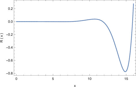
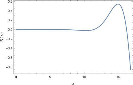
Figure 1: Comparison of the numerical solutions of the nonlinear biharmonic standing wave equation (55) and of the Laplace-Adomian Decomposition Method approximate solutions, truncated to three terms, given by Eq. (58. The numerical solution is represented by the solid curve, while the dashed curve depicts the Laplace-Adomian three terms solution. The initial conditions used to integrate the equations are $R(0)=5.1\times 10^{-5}$ and $R^{\prime\prime}(0)=2.65\times 10^{-5}$ (left figure), and $R(0)=-4.1\times 10^{-5}$ and $R^{\prime\prime}(0)=-7.86\times 10^{-6}$ (right figure), respectively.

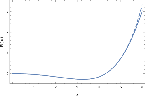
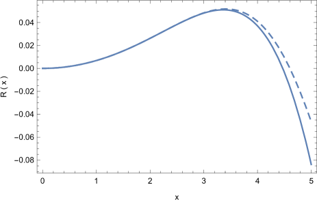
Figure 2: Comparison of the numerical solutions of the nonlinear biharmonic equation (55) and of the Adomian Decomposition Method approximate solutions, truncated to four terms, given by Eq. (73. The numerical solutions are represented by the solid curves, while the dashed curves depicts the Adomian Decomposition Method four terms solutions. The initial conditions used to integrate the equations are $R(0)=-4.1\times 10^{-6}$ and $R^{\prime\prime}(0)=-7.86\times 10^{-2}$ (left figure) and $R(0)=7.19\times 10^{-8}$ and $R^{\prime\prime}(0)=1.37\times 10^{-2}$ (right figure), respectively.

As one can see from Fig 1, the Laplace Adomian Decomposition Method, truncated to three terms only, gives an excellent description of the numerical solution, at least for the adopted range of initial conditions. The approximate solutions describes well the complex features of the solution on a relatively large range of the independent variable $x$. The simple Adomian Decomposition Method is more easy to apply, however, its accuracy seems to be limited, as compared to the Laplace Adomian Decomposition Method. Moreover, it is important to point out that there is a strong dependence on the initial conditions of the accuracy of the method. If the values $R(0)$ and $R^{\prime\prime}(0)$ are small, the series solutions are in good agreement with the numerical ones. However, for larger values of the initial conditions, the accuracy of the Adomian methods decreases rapidly.

III The biharmonic nonlinear equation with radial symmetry

In three dimensions $d=3$, and the radial biharmonic operator (18) takes the simple form

$$\Delta_{r}^{2}=\frac{d^{4}}{dr^{4}}+\frac{4}{r}\frac{d^{3}}{dr^{3}}.$$ (74)

Hence the general nonlinear three dimensional biharmonic equation with radial symmetry is given by

$$\frac{d^{4}y(r)}{dr^{4}}+\frac{4}{r}\frac{d^{3}y(r)}{dr^{3}}+\alpha\frac{d^{2}y(r)}{dr^{2}}+\frac{2}{r}\alpha\frac{dy(r)}{dr}+\omega y(r)+b^{2}+g(y(r))=f(r),$$ (75)

where $\alpha$, $b^{2}$ and $\omega$ are constants, while $g(y)$, the nonlinear operator term, and $f(r)$, are two arbitrary functions. Eq. (75) must be integrated with the initial conditions $y(0)=y_{0}$, $y^{\prime}(0)=y_{01}$, $y^{\prime\prime}(0)=y_{02}$, and $y^{\prime\prime\prime}(0)=y_{03}$, respectively. After multiplying Eq. (75) with $r$ we obtain

$$r\frac{d^{4}y(r)}{dr^{4}}+4\frac{d^{3}y(r)}{dr^{3}}+\alpha r\frac{d^{2}y(r)}{dr^{2}}+2\alpha\frac{dy(r)}{dr}+\omega ry(r)+rg(y(r))=rf(r)-b^{2}r.$$ (76)

III.1 The Laplace-Adomian Decomposition Method solution

As a first step in our study we assume that $y$ and $g(y(r))$ can be represented in the form of a power series as

$$y=\sum_{n=0}^{\infty}y_{n},g(y(r))=\sum_{n=0}^{\infty}A_{n},$$ (77)

where $A_{n}$ are the Adomian polynomials. Hence Eq. (76) becomes

$$\sum_{n=0}^{\infty}r\frac{d^{4}y_{n}(r)}{dr^{4}}+4\sum_{n=0}^{\infty}\frac{d^{3}y_{n}(r)}{dr^{3}}+\alpha\sum_{n=0}^{\infty}r\frac{d^{2}y_{n}(r)}{dr^{2}}+2\alpha\sum_{n=0}^{\infty}\frac{dy_{n}(r)}{dr}+$$

$$\omega\sum_{n=0}^{\infty}ry_{n}(r)+\sum_{n=0}^{\infty}rA_{n}=rf(r)-b^{2}r.$$ (78)

After applying the Laplace transformation operator to Eq. (76) we obtain

$$\sum_{n=0}^{\infty}\mathcal{L}\left[r\frac{d^{4}y_{n}(r)}{dr^{4}}\right]+4\sum_{n=0}^{\infty}\mathcal{L}\left[\frac{d^{3}y_{n}(r)}{dr^{3}}\right]+\alpha\sum_{n=0}^{\infty}\mathcal{L}\left[r\frac{d^{2}y_{n}(r)}{dr^{2}}\right]+2\alpha\sum_{n=0}^{\infty}\mathcal{L}\left[\frac{dy_{n}(r)}{dr}\right]+$$

$$\omega\sum_{n=0}^{\infty}\mathcal{L}\left[ry_{n}(r)\right]+\sum_{n=0}^{\infty}\mathcal{L}\left[rA_{n}\right]=\mathcal{L}\left[rf(r)-b^{2}r\right].$$ (79)

By taking into account the relations

$$\mathcal{L}\left[r\frac{d^{4}y_{n}(r)}{dr^{4}}\right](s)=\int_{0}^{\infty}r\frac{d^{4}y_{n}(r)}{dr^{4}}e^{-sr}dr=-\frac{d}{ds}\int_{0}^{\infty}\frac{d^{4}y_{n}(r)}{dr^{4}}e^{-sr}dr=-\frac{d}{ds}\mathcal{L}\left[\frac{d^{4}y_{n}(r)}{dr^{4}}\right](s),$$ (80)

$$\mathcal{L}\left[r\frac{d^{2}y_{n}(r)}{dr^{2}}\right]=\int_{0}^{\infty}r\frac{d^{2}y_{n}(r)}{dr^{2}}e^{-sr}dr=-\frac{d}{ds}\int_{0}^{\infty}\frac{d^{2}y_{n}(r)}{dr^{2}}e^{-sr}dr=-\frac{d}{ds}\mathcal{L}\left[\frac{d^{2}y_{n}(r)}{dr^{2}}\right](s),$$ (81)

$$\mathcal{L}\left[ry_{n}(r)\right](s)=\int_{0}^{\infty}ry_{n}(r)e^{-sr}dr=-\frac{d}{ds}\int_{0}^{\infty}y_{n}(r)e^{-sr}dr=-\frac{d}{ds}\mathcal{L}\left[y_{n}[(r)\right](s),$$ (82)

and the linearity of the Laplace transformation, Eq. (III.1) becomes

$$-\left(s^{4}+\alpha s^{2}+\omega\right)\sum_{n=0}^{\infty}F_{n}^{\prime}(s)-y(0)\left(\alpha+s^{2}\right)-2sy^{\prime}(0)-3y^{\prime\prime}(0)+$$

$$\sum_{n=0}^{\infty}\mathcal{L}\left[rA_{n}\right](s)=-\frac{b^{2}}{s^{2}}+\mathcal{L}\left[rf(r)\right](s).$$ (83)

From Eq. (III.1) we obtain the following recursion relations

$$-\left(s^{4}+\alpha s^{2}+\omega\right)F_{0}^{\prime}(s)-y(0)\left(\alpha+s^{2}\right)-2sy^{\prime}(0)-3y^{\prime\prime}(0)=-\frac{b^{2}}{s^{2}}+\mathcal{L}\left[rf(r)\right](s),$$ (84)

$$F_{n+1}^{\prime}(s)=\frac{1}{\left(s^{4}+\alpha s^{2}+\omega\right)}\mathcal{L}\left[rA_{n}\right](s).$$ (85)

From Eq. (84) we obtain

$$F_{0}(s)=\int G(s)ds,$$ (86)

where

$$G(s)=\frac{b^{2}/s^{2}-y(0)\left(\alpha+s^{2}\right)-2y^{\prime}(0)s-3y^{\prime\prime}(0)-\mathcal{L}\left[rf(r)\right](s)}{\left(s^{4}+\alpha s^{2}+\omega\right)},$$ (87)

while Eq. (85) gives

$$F_{k+1}(s)=\int\frac{1}{\left(s^{4}+\alpha s^{2}+\omega\right)}\mathcal{L}\left[rA_{k}\right](s)ds.$$ (88)

Hence we obtain the following approximate series solution of the radial nonlinear biharmonic equation (75),

$$y_{0}(r)=\mathcal{L}^{-1}\left[\int G(s)ds\right](r),$$ (89)

$$y_{k+1}=\mathcal{L}^{-1}\left\{\int\frac{1}{\left(s^{4}+\alpha s^{2}+\omega\right)}\mathcal{L}\left[rA_{k}\right](s)ds\right\}(r).$$ (90)

III.2 Application: the radial biharmonic standing wave equation

In radial symmetry, and by assuming that $R\in\mathbb{R}_{+}$, the standing wave equation (17) takes the form

$$\frac{d^{4}R(r)}{dr^{4}}+\frac{4}{r}\frac{d^{3}R(r)}{dr^{3}}+R(r)-R^{2\sigma+1}(r)=0,$$ (91)

or, equivalently,

$$r\frac{d^{4}R(r)}{dr^{4}}+4\frac{d^{3}R(r)}{dr^{3}}+rR(r)=rR^{2\sigma+1}(r).$$ (92)

By taking the Laplace transform of Eq. (92) we obtain

$$-\left(s^{4}+1\right)F^{\prime}(s)-R(0)s^{2}-2R^{\prime}(0)s-3R^{\prime\prime}(0)=\mathcal{L}\left[rR^{2\sigma+1}(r)\right](s).$$ (93)

By writing $R(r)=\sum_{n=0}^{\infty}R_{n}(r)$, $\mathcal{L}\left[R(r)\right](s)=\sum_{n=0}^{\infty}\mathcal{L}\left[R_{n}(r)\right](s)=\sum_{n=0}^{\infty}F_{n}(s)$, $R^{2\sigma+1}(r)=\sum_{n=0}^{\infty}A_{n}(r)$, Eq. (93) becomes

$$-\left(s^{4}+1\right)\sum_{n=0}^{\infty}F_{n}^{\prime}(s)-R(0)s^{2}-2R^{\prime}(0)s-3R^{\prime\prime}(0)=\sum_{n=0}^{\infty}\mathcal{L}\left[rA_{n}(r)\right](s).$$ (94)

Hence we obtain the following recursive relations for the solution of Eq. (91),

$$F_{0}^{\prime}(s)=-\frac{R(0)s^{2}+2R^{\prime}(0)s+3R^{\prime\prime}(0)}{s^{4}+1},$$ (95)

$$F_{k+1}^{\prime}(s)=-\frac{1}{s^{4}+1}\mathcal{L}\left[rA_{k}(r)\right](s).$$ (96)

Eq. (95) can be integrated exactly to obtain $F_{0}(s)$ as

$$F_{0}(s) = \frac{1}{8}\Bigg{\{}2\left[\sqrt{2}R(0)+4R^{\prime}(0)+3\sqrt{2}R^{\prime\prime}(0)\right]\tan^{-1}\left(1-\sqrt{2}s\right)-2\left[\sqrt{2}R(0)-4R^{\prime}(0)+3\sqrt{2}R^{\prime\prime}(0)\right]\times$$ (97)

$$\tan^{-1}\left(1+\sqrt{2}s\right)-\sqrt{2}\left[R(0)-3R^{\prime\prime}(0)\right]\ln\frac{s^{2}-\sqrt{2}s+1}{s^{2}+\sqrt{2}s+1}\Bigg{\}}.$$

In the following we will consider the solutions of Eq. (91) with $\sigma=1/2$, together with the initial conditions $R(0)\neq 0$, $R^{\prime}(0)=0$, $R^{\prime\prime}(0)\neq 0$, and $R^{\prime\prime\prime}(0)=0$, respectively. Then, by neglecting the non-linear term $R^{2}$ in Eq. (91) it turns out that the general solution of the linear equation

$$r\frac{d^{4}R_{0}(r)}{dr^{4}}+4\frac{d^{3}R_{0}(r)}{dr^{3}}+rR_{0}(r)=0,$$ (98)

is given by

$$R_{0}(r)=\frac{\left(\frac{1}{2}-\frac{i}{2}\right)\left\{\sin\left(\sqrt[4]{-1}r\right)\left[R(0)+3iR^{\prime\prime}(0)\right]+\sinh\left(\sqrt[4]{-1}r\right)\left[R(0)-3iR^{\prime\prime}(0)\right]\right\}}{\sqrt{2}r}.$$ (99)

The Laplace transform of $R_{0}$ converges only for values of $\mathrm{Re}\;s\geq s_{0}=1/\sqrt{2}$. In the region of convergence $F_{0}(s)$ can effectively be expressed as the absolutely convergent Laplace transform of another function, such that $F_{0}(s)=\left(s-s_{0}\right)\int_{0}^{\infty}{e^{-\left(s-s_{0}\right)t}\beta(t)dt}$, where $\beta(t)=\int_{0}^{t}{e^{-s_{0}u}R_{0}(u)du}$.

The first Adomian polynomial $A_{0}$ is obtained as $A_{0}(r)=R_{0}^{2}(r)$, and the Laplace transform of $rA_{0}$ is given by

$$\mathcal{L}\left[rA_{0}(r)\right](s) = \frac{1}{8}\Bigg{\{}3R(0)R^{\prime\prime}(0)\log\left(\frac{16}{s^{4}}+1\right)+\left[R(0)^{2}+9\left(R^{\prime\prime}(0)\right)^{2}\right]\ln\left(\frac{s^{2}+2}{s^{2}-2}\right)+$$ (100)

$$\left[R(0)^{2}-9\left(R^{\prime\prime}(0)\right)^{2}\right]\tan^{-1}\left(\frac{4}{s^{2}}\right)\Bigg{\}}.$$

Then the Laplace transform of the first correction term in the Adomian series expansion is given as the solution of the following differential equation,

$$F_{1}^{\prime}(s) = -\frac{1}{8\left(1+s^{4}\right)}\Bigg{\{}3R(0)R^{\prime\prime}(0)\log\left(\frac{16}{s^{4}}+1\right)+\left[R(0)^{2}+9\left(R^{\prime\prime}(0)\right)^{2}\right]\ln\left(\frac{s^{2}+2}{s^{2}-2}\right)+$$ (101)

$$\left[R(0)^{2}-9\left(R^{\prime\prime}(0)\right)^{2}\right]\tan^{-1}\left(\frac{4}{s^{2}}\right)\Bigg{\}}.$$

The right hand side of the above equation cannot be integrated exactly. By expanding it in power series of $1/s$, we obtain

$$F_{1}^{\prime}(s) \approx -\frac{R(0)^{2}}{s^{6}}-\frac{6(R(0)R^{\prime\prime}(0))}{s^{8}}+\frac{3R(0)^{2}-30\left(R^{\prime\prime}(0)\right)^{2}}{s^{10}}+\frac{54R(0)R^{\prime\prime}(0)}{s^{12}}+\frac{246\left(R^{\prime\prime}(0)\right)^{2}-\frac{151R(0)^{2}}{5}}{s^{14}}-$$ (102)

$$\frac{566(R(0)R^{\prime\prime}(0))}{s^{16}}+O\left(\left(\frac{1}{s}\right)^{17}\right),$$

and

$$F_{1}(s) \approx \frac{1}{5}\Bigg{\{}\frac{566R(0)R^{\prime\prime}(0)}{3s^{15}}+\frac{151R(0)^{2}-1230\left(R^{\prime\prime}(0)\right)^{2}}{13s^{13}}-\frac{270R(0)R^{\prime\prime}(0)}{11s^{11}}-\frac{5\left[R(0)^{2}-10\left(R^{\prime\prime}(0)\right)^{2}\right]}{3s^{9}}+$$ (103)

$$\frac{30R(0)R^{\prime\prime}(0)}{7s^{7}}+\frac{R(0)^{2}}{s^{5}}\Bigg{\}}.$$

respectively. Hence for the first term of the Adomian series expansion $R_{1}=\mathcal{L}^{-1}\left[F_{1}(s)\right](r)$ we obtain

$$R_{1}(r) = \frac{R(0)^{2}}{120}r^{4}+\frac{1}{840}R(0)R^{\prime\prime}(0)r^{6}+\frac{10\left(R^{\prime\prime}(0)\right)^{2}-R(0)^{2}}{120960}r^{8}-\frac{R(0)R^{\prime\prime}(0)}{739200}r^{10}+$$ (104)

$$\frac{151R(0)^{2}-1230\left(R^{\prime\prime}(0)\right)^{2}}{31135104000}r^{12}+\frac{283R(0)R^{\prime\prime}(0)}{653837184000}r^{14}+....$$

The comparison of the two terms truncated Laplace-Adomian Decomposition Method solution, $R(r)\approx R_{0}(r)+R_{1}(r)$ with the exact numerical solution is presented, for two different sets of initial conditions, in Fig. 3.

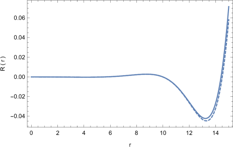
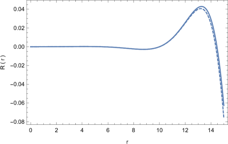
Figure 3: Comparison of the numerical solutions of the radial biharmonic standing wave equation (91) and of the approximate solutions obtained by the Laplace-Adomian Decomposition Method, truncated to two terms, $R(r)\approx R_{0}(r0+R_{1}(r)$. The numerical solutions are represented by the solid curves, while the dashed curves depicts the Laplace-Adomian Decomposition Method two terms solutions. The initial conditions used to integrate the equations are $R(0)=-7.85\times 10^{-12}$ and $R^{\prime\prime}(0)=-4.31\times 10^{-5}$ (left figure) and $R(0)=1.27\times 10^{-12}$ and $R^{\prime\prime}(0)=4.31\times 10^{-5}$ (right figure), respectively.

III.3 The Adomian Decomposition Method for the radial biharmonic standing waves equation

We consider now the use of the Adomian Decomposition Method for obtaining a semi-analytical solution of the radial biharmonic standing waves equation. For the sake of generality we will consider a more general equation of the form

$$\frac{d^{4}R}{dr^{4}}+f\left(r\right)\frac{d^{3}R}{dr^{3}}=R^{2\sigma+1}-R,$$ (105)

where $f(r)$ is an arbitrary function of the radial coordinate $r$, and which we will solve with the initial conditions $R(0)\neq 0$, $R^{\prime}\left(0\right)=0$, $R^{\prime\prime}\left(0\right)\neq 0$, and $R^{\prime\prime\prime}(0)=0$, respectively. Then the following identity can be immediately obtained,

$$\int_{0}^{r}dr_{1}\int_{0}^{r_{1}}dr_{2}\int_{0}^{r_{2}}e^{-\int f\left(r_{3}\right)dr_{3}}dr_{3}\int_{0}^{r_{3}}e^{\int f\left(r_{4}\right)dr_{4}}\left[R^{\prime\prime\prime\prime}\left(r_{4}\right)+f\left(r_{4}\right)R^{\prime\prime\prime}\left(r_{4}\right)\right]dr_{4}$$ (106)

$$= \int_{0}^{r}dr_{1}\int_{0}^{r_{1}}dr_{2}\int_{0}^{r_{2}}e^{-\int f\left(r_{3}\right)dr_{3}}dr_{3}\left[\int_{0}^{r_{3}}e^{\int f\left(r_{4}\right)dr_{4}}dR^{\prime\prime\prime\prime}\left(r_{4}\right)+\int_{0}^{r_{3}}e^{\int f\left(r_{4}\right)dr_{4}}f\left(r_{4}\right)R^{\prime\prime\prime}\left(r_{4}\right)dr_{4}\right]$$

$$= \int_{0}^{r}dr_{1}\int_{0}^{r_{1}}dr_{2}\int_{0}^{r_{2}}e^{-\int f\left(r_{3}\right)dr_{3}}\left[\int_{0}^{r_{3}}d\left(e^{\int f\left(r\right)dr}R^{\prime\prime\prime}\left(r\right)\right)\right]dr_{3}$$

$$= \int_{0}^{r}dr_{1}\int_{0}^{r_{1}}dr_{2}\int_{0}^{r_{2}}e^{-\int f\left(r_{3}\right)dr_{3}}\left.\left(e^{\int f\left(r\right)dr}R^{\prime\prime\prime}\left(r\right)\right)\right|_{r=0}^{r=r_{3}}dr_{3}$$

$$= \int_{0}^{r}dr_{1}\int_{0}^{r_{1}}dr_{2}\int_{0}^{r_{2}}e^{-\int f\left(r_{3}\right)dr_{3}}e^{\int f\left(r_{3}\right)dr_{3}}R^{\prime\prime\prime}\left(r_{3}\right)dr_{3}=\int_{0}^{r}dr_{1}\int_{0}^{r_{1}}dr_{2}\int_{0}^{r_{2}}R^{\prime\prime\prime}\left(r_{3}\right)dr_{3}$$

$$= R\left(r\right)-R\left(0\right)-R^{\prime\prime}\left(0\right)\frac{r^{2}}{2}.$$

Thus Eq. (105) can be reformulated as an equivalent integral equation given by

$$R\left(r\right)=R\left(0\right)+R^{\prime\prime}\left(0\right)\frac{r^{2}}{2}+\int_{0}^{r}dr_{1}\int_{0}^{r_{1}}dr_{2}\int_{0}^{r_{2}}e^{-\int f\left(r_{3}\right)dr_{3}}dr_{3}\int_{0}^{r_{3}}e^{\int f\left(r_{4}\right)dr_{4}}\left[R^{2\sigma+1}\left(r_{4}\right)-R\left(r_{4}\right)\right]dr_{4}.$$ (107)

By taking into account that $f(r)=4/r$, and by decomposing $R$ and $R^{2\sigma+1}$ as $R=\sum_{n=0}^{\infty}{R_{n}}$ and $R^{2\sigma+1}=\sum_{n=0}^{\infty}{A_{n}}$, where $A_{n}$ are the Adomian polynomials, we obtain

$$R_{0}\left(r\right)+\sum_{n=0}^{\infty}R_{n+1}\left(r\right)=R\left(0\right)+R^{\prime\prime}\left(0\right)\frac{r^{2}}{2}+\int_{0}^{r}dr_{1}\int_{0}^{r_{1}}dr_{2}\int_{0}^{r_{2}}\frac{1}{r_{3}^{4}}dr_{3}\int_{0}^{r_{3}}r_{4}^{4}\left[\sum_{n=0}^{\infty}A_{n}\left(r_{4}\right)-\sum_{n=0}^{\infty}R_{n}\left(r_{4}\right)\right]dr_{4}.$$ (108)

Then an analytic solution to Eq. (105) can be obtained with the help of the recursive relations

$$R_{0}\left(r\right)=R\left(0\right)+R^{\prime\prime}\left(0\right)\frac{r^{2}}{2},$$ (109)

$$R_{k+1}\left(r\right)=\int_{0}^{r}dr_{1}\int_{0}^{r_{1}}dr_{2}\int_{0}^{r_{2}}\frac{1}{r_{3}^{4}}dr_{3}\int_{0}^{r_{3}}r_{4}^{4}\left[A_{k}\left(r_{4}\right)-R_{k}\left(r_{4}\right)\right]dr_{4}.$$ (110)

III.3.1 Application: the case $\sigma=1/2$

As an application of the Adomian Decomposition Method for obtaining the solution of Eq. (105) we consider the case $\sigma=1/2$. Hence the radial biharmonic standing wave equation becomes

$$\frac{d^{4}R}{dr^{4}}+\frac{4}{r}\frac{d^{3}R}{dr^{3}}=R^{2}-R.$$ (111)

The first few terms in the series solution of this equation are given by

$$R_{0}\left(r\right)=R\left(0\right)+R^{\prime\prime}\left(0\right)\frac{r^{2}}{2},$$ (112)

$$R_{1}(r)=\frac{1}{120}\left[R(0)-1\right]R(0)r^{4}+\frac{\left[2R(0)-1\right]R^{\prime\prime}(0)}{1680}r^{6}+\frac{\left(R^{\prime\prime}(0)\right)^{2}}{12096}r^{8},$$ (113)

$$R_{2}(r) = \frac{R(0)\left[2R(0)^{2}-3R(0)+1\right]}{362880}r^{8}+\frac{\left[18R(0)^{2}-18R(0)+1\right]R^{\prime\prime}(0)}{13305600}r^{10}+\frac{41\left[2R(0)-1\right]\left(R^{\prime\prime}(0)\right)^{2}}{1037836800}r^{12}+$$ (114)

$$\frac{\left(R^{\prime\prime}(0)\right)^{3}}{396264960}r^{14},$$

$$R_{3}(r) = \frac{R(0)\left[146R(0)^{3}-292R(0)^{2}+151R(0)-5\right]}{31135104000}r^{12}+\frac{\left[1120R(0)^{3}-1680R(0)^{2}+566R(0)-3\right]R^{\prime\prime}(0)}{1307674368000}r^{14}+$$ (115)

$$\frac{\left[31282R(0)^{2}-31282R(0)+3407\right]\left(R^{\prime\prime}(0)\right)^{2}}{414968666112000}r^{16}+\frac{3061\left[2R(0)-1\right]\left(R^{\prime\prime}(0)\right)^{3}}{2027418340147200}r^{18}+$$

$$\frac{89\left(R^{\prime\prime}(0)\right)^{4}}{1366067972505600}r^{20}.$$

The comparison between the exact numerical solution and the approximate solution $R(r)=R_{0}(r)+R_{1}(r)+R_{2}(r)+R_{3}(r)$ of Eq. (111) is represented, for two sets of initial values, in Fig. 4.

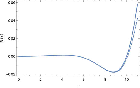
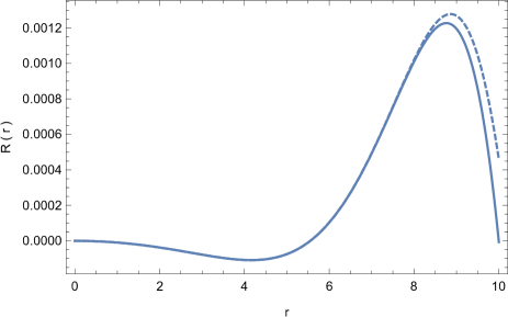
Figure 4: Comparison of the numerical solutions of the radial biharmonic standing wave equation (111) and of the Adomian Decomposition Method approximate solutions, truncated to four terms. The numerical solutions are represented by the solid curves, while the dashed curves depicts the Adomian Decomposition Method four terms solutions. The initial conditions used to integrate the equations are $R(0)=7.44\times 10^{-15}$ and $R^{\prime\prime}(0)=2.71\times 10^{-4}$ (left figure) and $R(0)=-3.89\times 10^{-16}$ and $R^{\prime\prime}(0)=-1.91\times 10^{-5}$ (right figure), respectively.

IV Discussions and concluding remarks

In the present paper we have presented the applications of the Adomian Decomposition method for solving the nonlinear biharmonic differential equation. The Adomian Decomposition Method has been successfully used to solve many classes of differential, integral and functional equations. It has also important applications in science and engineering. The basic ingredient of this approach is the decomposition of the nonlinear term in the differential equations into a series of polynomials of the form $\sum_{n=1}^{\infty}{A_{n}}$, where $A_{n}$ are the so-called Adomian polynomials. Simple formulas that can generate Adomian polynomials for many forms of nonlinearity have been derived in R1 ; R2 . The solutions of the nonlinear differential equations can be obtained recursively, and each term of the Adomian series can be computed once the corresponding polynomial, obtained from an expansion of the nonlinear term into a power series, is known.

We have considered in detail both the one dimensional, as well as the radial, three dimensional, biharmonic type equation containing some nonlinear terms. We have implemented two versions of the Adomian Decomposition Method for solving the biharmonic equation, namely, the Laplace-Adomian Decomposition Method, and the standard Adomian Decomposition Method. The Laplace-Adomian Decomposition Method combines the powerful Laplace transformation with the advantages of the Adomian method, with the iterative procedure applied in the space of the Laplace transformed functions. In the radial case the Laplace transforms of the terms in the Adomian expansion can be obtained as solutions of a first order differential equation, which can be obtained by quadratures. However, in the present case the integral, and the Laplace transform itself, cannot be obtained in an exact form, and therefore one have to resort to some approximate methods.

For each type of considered equations we have also considered some concrete examples, and we have compared the Adomian solution with the exact numerical solution. Generally, the efficiency and the precision of the Laplace-Adomian Decomposition Method is very good. In the case of the one-dimensional standing wave biharmonic equation only three terms of the Adomian expansion are enough to give a good approximation of the numerical solution, while for the case of the radial nonlinear biharmonic standing wave equation the numerical solution can be approximated by using only two terms. This coincidence implicitly shows the power of the Adomian method, which can be used to find out even the exact solution of a given differential equation. However, in general the application of the method may be complicated by the difficulties in solving exactly the differential equations for the Laplace transform, and for obtaining the inverse Laplace transform. But, at least in the case of the radial nonlinear standing wave equation, a simple technique based on the power series expansion of the Laplace transform of the Adomian polynomials gives good approximations of the numerical solutions. Numerical techniques for obtaining the inverse Laplace transform Lern may also be useful in obtaining the successive terms in the Laplace-Adomian expansion.

We have also considered the standard Adomian Decomposition Method for both the first order and radial nonlinear biharmonic equations. Computationally, this method is very simple, and it can provide some power series solutions that can describe the numerical solution relatively well. The Adomian method is very simple and efficient, but it may raise some questions about the convergence of the series of functions C1 ; C2 . Moreover, we must point out that the accuracy of the approximations of the numerical solution by the Adomian series is strongly dependent on the initial conditions used to solve the equations. The Adomian solutions work well for small numerical values of the initial conditions. Once these values are increased, the accuracy of the estimations becomes poor, at least for the number of terms used to approximate the solutions in the present approach. These raises the issue of the dependence of the convergence of the Adomian solution from the initial conditions, a mathematical problem certainly worth of investigating.

The biharmonic equation appears in many physical and engineering applications Bose1 ; Boos ; n1 ; n2 . In particular, it plays an important role within the hydrodynamic formulation of the Schrödinger equation, and in the presence of the quantum potential. This physical approach is extensively used for the study of the quantum fluids. In many applications, mostly due to the computational difficulties, the quantum potential is neglected. However, by using the present approach, semi-analytical solutions of the biharmonic equation can be obtained, which can approximate well the numerical solution. The semi-analytical solutions offer the possibility of a deeper insight into the physical nature of the problem, as well as of a significant simplification of the estimation of some relevant physical parameters. Similar applications of the method could lead to the development of powerful mathematical methods for solving different problems described by fourth order differential equations that play an important role in engineering, like, for example, in the study of the large amplitude free vibrations of a uniform cantilever beam Bel .

The Adomian Decomposition Method, as well as its Laplace transform version, represents a powerful mathematical tool for physicists and engineers investigating both theoretical and applied problems. The biharmonic equation, and its extensions, are interesting in themselves from a mathematical point of view. There are also important in many applications. In the present study we have introduced some theoretical tools, which are extremely effective in dealing with strongly nonlinear differential equations and complex mathematical models, and that may help in the better understanding of the properties and solutions of the nonlinear biharmonic equation.

References

• (1) K. Abbaoui and Y. Cherrualt, Convergence of the Adomians method applied to differential equations, Comp. Math. Appl. 28 (1994), 103-109.
• (2) K. Abbaoui and Y. Cherrualt, Convergence of the Adomians method applied to nonlinear equations, Math. Comp. Mod. 20 (1994), 69-73.
• (3) G. Adomian, Decomposition solution for Duffing and Van der Pal oscillators, Int. J. Math. & Math. Sci. 9 (1986), 731-732.
• (4) G. Adomian, Convergent series solution of nonlinear equations, J. Comput. Appl. Math. 11 (1984), 225-230.
• (5) G. Adomian, On the convergence region for decomposition solutions, J. Comput. Appl. Math. 11 (1984), 379-380.
• (6) G. Adomian, Nonlinear stochastic dynamical systems in physical problems, J. Math. Anal. Appl. 111 (1985), 105-113.
• (7) G. Adomian, A review of the Decomposition Method in Applied Mathematics, J. Math. Anal. Appl. 135 (1988), 501-544.
• (8) G. Adomian, Solving Frontier Problems of Physics: the Decomposition Method, Kluwer, Dordrecht, The Netherlands, 1994.
• (9) G. Adomian, R. Rach, Modified Adomian Polynomials, Math. Comp. Mod. 24 (1996), 39-46.
• (10) E. Babolian, S. Javadi, Restarted Adomian Method for Algebraic Equations, Appl. Math. Comput. 146 (2003), 533-541.
• (11) E. Babolian, S. Javadi, H. Sadehi, Restarted Adomian Method for Integral Equations, Appl. Math. Comput. 153 (2004), 353-359.
• (12) H. O. Bakodah, Some Modification of the Adomian Decomposition Method Applied to Nonlinear System of Fredholm Integral Equations of the Second Kind, Int. J. Contemp. Math. Sciences, 7 (2012), 929-942.
• (13) G. Baruch, G. Fibich, and E. Mandelbaum, Singular solutions of the biharmonic Nonlinear Schrödinger equation, Nonlinearity 70 (2010), 3319-3341. (2009).
• (14) G. Baruch, G. Fibich, E. Mandelbaum, Ring-type singular solutions of the biharmonic nonlinear Schrödinger equation, Nonlinearity 23 (2010), 2867-2887.
• (15) G. Baruch and G. Fibich, Singular solutions of the $L^{2}$-supercritical biharmonic nonlinear Schrödinger equation, Nonlinearity 24 (2011), 1843-1859.
• (16) J. A. Belinchon, T. Harko, and M. K. Mak, Approximate Analytical Solution for the Dynamic Model of Large Amplitude Non-Linear Oscillations Arising in Structural Engineering, J. Applied Math. Eng. 8 (2016), 25-34.
• (17) J. Biazar, E. Babolian, R. Islam, Solution of the System of Ordinary Differential Equations by Adomian Decomposition Method, Appl. Math. Comput. 147 (2004), 713-719.
• (18) J. Biazar, E. Babolian, A. Nouri, R. Islam, An Alternate Algorithm for Computing Adomian Decomposition Method in Special Cases, Appl. Math. Comput. 138 (2003), 523-529.
• (19) J. Biazar, M. Tango, E. Babolian, R. Islam, Solution of the Kinetic Modeling of Lactic Acid Fermentation Using Adomian Decomposition Method, Appl. Math. Comput. 144 (2003), 433-439.
• (20) C. G. Boehmer and T. Harko, Can dark matter be a Bose-Einstein condensate?, JCAP 06 (2007), 025.
• (21) J. Boos, Gravitational Friedel oscillations in higher-derivative and infinite-derivative gravity?, Int. J. Mod. Phys. D 27 (2018), 1847022.
• (22) K. T. Chau, Theory of Differential Equations in Engineering in Mechanics, CRC Press Taylor & Francis Group, Boca Raton, USA, 2018.
• (23) Y. Cherruault, G. Adomian, K. Abbaoui, R. Rach, Further Remarks on Convergence of Decomposition Method, Int. J. Bio-Med. Comp. 38 (1995), 89-93.
• (24) H. Fatoorehchi, R. Zarghami, H. Abolghasemi, and R. Rach, Chaos control in the cerium-catalyzed Belousov-Zhabotinsky reaction using recurrence quantification analysis measures, Chaos, Solitons & Fractals 76 (2015), 121-129.
• (25) G. Fibich and G. C. Papanicolaou, Self-focusing in the perturbed and unperturbed nonlinear Schrödinger equation in critical dimension, SIAM J. Applied Math. 60 (1999), 183-240.
• (26) G. Fibich, B. Ilan, and G. Papanicolaou, Self-focusing with fourth-order dispersion, SIAM J. Applied Math. 62 (2002), 1437-1462.
• (27) H. Ghasemi, M. Ghovatmand, S. Zarrinkamar, and H. Hassanabadi, Solution of the nonlinear Klein-Gordon equation for two new terms via the Adomian decomposition method, Eur. Phys. J. Plus 129 (2014), 32.
• (28) T. Harko, Evolution of cosmological perturbations in Bose-Einstein condensate dark matter, Mon. Not. Roy. Astron. Soc. 413 (2011), 3095-3104.
• (29) T. Harko, Bose-Einstein condensation of dark matter solves the core/cusp problem, JCAP 05 (2011), 022.
• (30) T. Harko and G. Mocanu, Cosmological evolution of finite temperature Bose-Einstein condensate dark matter, Phys. Rev. D 85 (2012), 084012.
• (31) N. Hayashi, J. A. Mendez-Navarro, and P. I. Naumkin, Asymptotics for the fourth-order nonlinear Schrödinger equation in the critical case, J. Diff. Eqs. 261 (2016), 5144-5179.
• (32) S. He, K. Sun, and S. Banerjee, Dynamical properties and complexity in fractional-order diffusionless Lorenz system, Eur. Phys. J. Plus 131 (2016), 254.
• (33) S. He, K. Sun, X. Mei, B. Yan, and S. Xu, Numerical analysis of a fractional-order chaotic system based on conformable fractional-order derivative, Eur. Phys. J. Plus 132 (2017), 36.
• (34) H. Jafari, V. Daftardar-Gejji, Revised Adomian Decomposition Method for Solving a System of Nonlinear Equations, Appl. Math. Comput. 175 (2006), 1-7.
• (35) H. Jafari, V. Daftardar-Gejji, Revised Adomian Decomposition Method for Solving a System of Ordinary and Fractional Differential Equations, Appl. Math. Comput. 181 (2006), 598-608.
• (36) C. Jin, M. Liu, A New Modification of Adomian Decomposition Method for Solving a Kind of Evolution Equations, Appl. Math. Comput. 169 (2005), 953-962.
• (37) A. K. Khalifa, The decomposition method for one dimensional biharmonic equations, Int. J. Sim. Proc. Mod. 2 (2006), 33-36.
• (38) L. D. Landau & E. M. Lifshitz, Theory of Elasticity, Pergamon Press, Oxford, UK, 1970.
• (39) D. M. Lerner and G. M. Lerner, A simplified algorithm for the inverse Laplace transform, Radiophysics and Quantum Electronics 13 (1970), 482-484.
• (40) X.-G. Luo, A Two-Step Adomian Decomposition Method, Appl. Math. Comput. 170 (2005), 570-583.
• (41) M. K. Mak, C. S. Leung, and T. Harko, Computation of the general relativistic perihelion precession and of light deflection via the Laplace-Adomian Decomposition Method, Adv. High En. Phys. 2018 (2018), 7093592.
• (42) M. Marin, Contributions on uniqueness in thermoelastodynamics on bodies with voids, Cienc. Mat.(Havana) 16 (1998), 101-109.
• (43) M. Marin, An evolutionary equation in thermoelasticity of dipolar bodies, J. Math. Phys. 40 (1999), 1391-1399.
• (44) M. Marin and O. Florea, On temporal behaviour of solutions in thermoelasticity of porous micropolar bodies, An. St. Univ. Ovidius Constanta-Seria Mathematics 22 (2014), 169-188.
• (45) S. T. Mohyud-Din, W. Sikander, U. Khan, and N. Ahmed, Optimal variational iteration method using Adomian's polynomials for physical problems on finite and semi-infinite intervals, Eur. Phys. J. Plus 132 (2017), 236.
• (46) M. M. Mousa and M. Reda, The Method of Lines and Adomian Decomposition for Obtaining Solitary Wave Solutions of the KdV Equation, Applied Physics Research 5 (2013), 43-57.
• (47) P. I. Naumkin and J. J. Perez, Higher-order derivative nonlinear Schrödinger equation in the critical case, J. Math. Phys. 59 (2018), 021506.
• (48) K. Parand, J. A. Rad, and M. Ahmadi, A comparison of numerical and semi-analytical methods for the case of heat transfer equations arising in porous medium, Eur. Phys. J. Plus 131 (2016), 300.
• (49) B. Pausader and S. Xia, Scattering theory for the fourth-order Schrödinger equation in low dimensions, Nonlinearity 26 (2013), 2175-2191.
• (50) R. Rach, G. Adomian, R. E. Meyers, A modified decomposition, Comp. & Math. Appl. 23 (1992), 17-23.
• (51) J. Ruan, K. Sun, J. Mou, S. He, and L. Zhang, Fractional-order simplest memristor-based chaotic circuit with new derivative, Eur. Phys. J. Plus 133 (2018), 3.
• (52) J. Ruan and Z. Lu, A modified algorithm for the Adomian decomposition method with applications to Lotka-Volterra systems, Math. Comput. Mod. 46 (2007), 1214-1224.
• (53) M. Ruzicka, Electrorheological Fluids: Modeling and Mathematical Theory (Lecture Notes in Mathematics: 1748), Springer Verlag, Berlin, Heidelberg, New York, 2000.
• (54) A. P. S. Selvadurai, Partial Differential Equations in Mechanics, Vol. 2, The Biharmonic Equation, Poisson's Equation, Springer Verlag, Berlin Heidelberg New York, 2000.
• (55) Ch. Tsitouras, Rational Approximants to the Solution of the Brusselator System compared to the Adomian Decomposition Method, Int. J. Contemp. Math. Sciences 4 (2009), 815-820.
• (56) L. Visinelli, Condensation of Galactic Cold Dark Matter, JCAP 1607 (2016), 009.
• (57) A.-M. Wazwaz, The Modified Decomposition Method and Padé Approximation for Solving the Thomas-Fermi Equation, Appl. Math. Comput. 105 (1999), 11-19.
• (58) A.-M. Wazwaz, A Reliable Modification of Adomian Decomposition Method, Appl. Math. Comput. 102 (1999), 77-86.
• (59) A.-M. Wazwaz, S. M. El-sayed, A New Modification of the Adomian Decomposition Method for Linear and Nonlinear Operators, Appl. Math. Comput. 122 (2001), 393-405.
• (60) A.-M. Wazwaz, Adomian Decomposition Method for a reliable treatment of the Edman-Flower equation, Appl. Math. Comput. 161 (2005), 543-560.
• (61) A.-M. Wazwaz, Adomian Decomposition Method for a reliable treatment of the Bratu type equation, Appl. Math. Comput. 166 (2005), 652-663.
• (62) Y. Xu, K. Sun, S. He, and L. Zhang, Dynamics of a fractional-order simplified unified system based on the Adomian decomposition method, Eur. Phys. J. Plus 131 (2016), 186.
• (63) B.-Q. Zhang, Q.-B. Wu, X.-G. Luo, Experimentation with Two-Step Adomian Decomposition Method to Solve Evolution Models, Appl. Math. Comput. 175 (2006), 1495-1502.
• (64) L. Zhang, K. Sun, S. He, H. Wang, and Y. Xu, Solution and dynamics of a fractional-order 5-D hyperchaotic system with four wings, Eur. Phys. J. Plus 132 (2017), 31.