A Weakly Supervised Approach for Estimating Spatial Density Functions from High-Resolution Satellite Imagery

Abstract.

We propose a neural network component, the regional aggregation layer, that makes it possible to train a pixel-level density estimator using only coarse-grained density aggregates, which reflect the number of objects in an image region. Our approach is simple to use and does not require domain-specific assumptions about the nature of the density function. We evaluate our approach on several synthetic datasets. In addition, we use this approach to learn to estimate high-resolution population and housing density from satellite imagery. In all cases, we find that our approach results in better density estimates than a commonly used baseline. We also show how our housing density estimator can be used to classify buildings as residential or non-residential.

1. Introduction

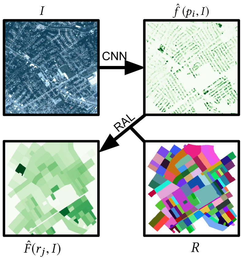
Figure 1. We use a CNN to generate a pixel-level density map (top-right) from an input satellite image (top-left). We introduce the regional aggregation layer (RAL), which explicitly models the aggregation process for a given set of regions (bottom-right), to generate the corresponding spatially aggregated densities (bottom-left). This enables us to train the CNN using only aggregated densities as ground truth.

The availability of high-resolution, high-cadence satellite imagery has revolutionized our ability to photograph the world and how it changes over time. Recently, the use of convolutional neural networks (CNNs) has made it possible to automatically extract a wide variety of information from such imagery at scale. In this work, we focus on using CNNs to make high-resolution estimates of the distribution of human population and housing from satellite imagery. Understanding changes in these distributions is critical for many applications, from urban planning to disaster response. Several specialized systems that estimate population/housing distributions have been developed, including LandScan (Dobson et al., 2000) and the High Resolution Settlement Layer (Facebook Connectivity Lab and Center for International Earth Science Information Network, Columbia University, 2016). While our work addresses the same task, our approach should be considered as a component that could be integrated into such a system rather than a direct competitor.

Our method can be used to train a CNN to estimate any high-resolution geospatial density function from satellite imagery. The key challenge in training such models is that data that reflects geospatial densities is often coarse grained, provided as aggregates over large spatial regions instead of at the pixel-level grid of the available imagery. This means that traditional methods for training CNNs to make pixel-level predictions will not work. To overcome this, we propose a weakly supervised learning strategy, where we use the available coarse-grained labels to learn to make fine-grained predictions. With our method, we can train a CNN to generate a high-spatial resolution output, at the pixel-level if desired, using only labels that represent aggregates over spatial regions. See Figure 1 for a visual overview of our approach.

Many methods for disaggregating spatial data have been developed to address this problem, one of the most prominent is called dasymetric mapping (Wright, 1936). The key downside of this approach is that it requires aggregated sums at inference time. It also typically involves significant domain-specific assumptions and intimate knowledge of the input data and imagery. In contrast, we propose an end-to-end strategy for learning to predict the disaggregated densities which makes minimal assumptions and can be applied to a wide variety of input data. In addition, our method only requires aggregated sums during the CNN training phase. During inference, only a single forward pass through the CNN is required to estimate the spatial density. It is also possible, if the aggregated sums are available at inference time, to incorporate them using dasymetric mapping techniques.

Our approach is easy to apply and operates quickly at training and inference time, especially using modern GPU hardware. At training time, there is a small amount of overhead, because we need to compute an estimate of the aggregated densities, but at inference time no additional computation is required. In addition, our approach is quite general, and could naturally be extended to area-wise averaging and other aggregation operations, such as regional maximization. The only requirement is that the aggregation operation must be differentiable w.r.t. the input density map. Critically, it is not required that the aggregation operation be differentiable w.r.t. any parameters of the aggregation operation (e.g., the layout of the spatial regions).

The main contributions of this work include: (1) proposing an end-to-end optimizable method that makes it possible to train a CNN that generates pixel-level density estimates using aggregated densities of arbitrary regions; (2) an evaluation of this method, with various extensions, including different regularization schemes on synthetic data; (3) an evaluation of this method on a large-scale dataset of satellite imagery for the tasks of population and housing density estimation; (4) a demonstration of its use as a method for dasymetric mapping, which is useful if aggregated sums are available for the test data; and (5) a demonstration of how we can use our high-resolution housing density estimates, in conjunction with an existing building segmentation CNN, to perform residential vs. non-residential building segmentation.

2. Related Work

Over the past ten years, the use of deep convolutional neural networks has rapidly advanced the state of the art on many tasks in the field of computer vision. For example, the top-1 accuracy for the well-known ImageNet dataset (Russakovsky et al., 2015) (ILSVRC-2012 validation set) has risen from around $60\%$ in 2012 (Krizhevsky et al., 2012) to $82.7\%$ in 2018 (Zoph et al., 2018). Significant improvements, using similar methods, have been achieved in object detection (Redmon and Farhadi, 2017), semantic segmentation (Ronneberger et al., 2015; Zhao et al., 2017; Peng et al., 2017; Chen et al., 2018b), and instance segmentation (He et al., 2017; Chen et al., 2018a). Recently, these methods have been applied to traditional remote sensing tasks, largely by adapting methods initially developed in the computer vision community. Notable examples include applications to land cover segmentation (Kussul et al., 2017b; Pascual et al., 2018), land degradation estimation (Kussul et al., 2017a), and crop classification (Ji et al., 2018; Bargiel, 2017).

2.1. Weakly Supervised Learning

In traditional machine learning, we are given strong labels, which directly correspond to the desired output. In weakly supervised learning, the provided labels are coarser grained, either semantically or spatially, and potentially noisy. For example, Zhou et al. (Zhou et al., 2016) introduce a discriminative localization method that uses image-level labels, intended for classification training, to enable object localization and detection using a global average pooling (GAP) (Lin et al., 2013) layer. Khoreva et al. present a weak supervision method for training a pixel-level semantic segmentation CNN, using only bounding boxes (Khoreva et al., 2017). Zhou et al. (Zhou et al., 2018) show that image-level labels can be used for instance and semantic segmentation by finding peak responses in convolutional feature maps. In this paper, we have supervision of coarse spatial labels but we want to predict fine, per-pixel prediction without access to such data for training.

The technique we propose is most closely related to the use of a GAP layer for discriminative object localization (Zhou et al., 2016). The idea in the previous work is to have a fully convolutional CNN output per-pixel logits, average these logits across the entire image, and then pass the averaged logits through a softmax to estimate a distribution over the desired class labels. Once this network is trained, it is possible to modify the network architecture to extract the pixel-level logits and use them for object localization. This is a straightforward process because the GAP layer is linear. Our proposed regional aggregation layer (RAL) is also linear, but aggregates values from sub-regions of the image, which is critical because of significant variability in region sizes and shapes. Since our focus is on estimating a pixel-level density using aggregated densities, we perform aggregation on a single channel at a time and omit the softmax. Similarly to the previous work, after our network is trained, we can use the intermediate pixel-level outputs to extract the desired information at the pixel level.

2.2. Image-Based Counting

An important application that has received comparatively less attention is that of image-based counting. Broadly, there are two categories of image-based counting techniques: direct and indirect. Direct counting methods are usually based on object detection, semantic segmentation, or subitizing. Indirect methods are trained to predict object densities which can be used to estimate the count in an image. Typical object detection/segmentation based methods used for counting have to exactly locate each instance of an object which is a challenging task due to varying scales of objects in images. Several methods formulate counting as a subitizing problem, inspired by ability of humans to estimate the count of objects without explicitly counting. Zhang et al. (Zhang et al., 2015) proposed a class-agnostic object-counting method, salient object subitizing, which uses a CNN to predict image-level object counts. The work by Chattopadhyay et al. (Chattopadhyay et al., 2017) tackles multiple challenges including multi-class counting in a single image and varying scales of objects. These methods require strongly-annotated training data. Gao et al. (Gao et al., 2018) propose a weakly supervised framework that uses the known count of objects in images to enable object localization.

Density-based counting methods are generally used to tackle applications which have a large number of objects and drastically varying scales of object instances. For example, in crowd counting, a person might span hundreds of pixels if they are close to the camera or only a few if they are in the distance and occluded by others. Regardless, both must be counted. Recent CNN-based methods have been shown to provide state-of-the-art results on large-scale crowd counting. Hydra CNN (Onoro-Rubio and López-Sastre, 2016) is a density estimation method based on image patches. A contextual pyramid CNN by Sindagi and Patel (Sindagi and Patel, 2017) leverages global and local context for crowd density estimation. In the previous work, counting is formulated so that all the density values in an image should sum up to the count of objects. Our work is similar in that we predict pixel-level densities, but we focus on estimating densities from overhead views and using arbitrarily defined regions as training data.

2.3. Dasymetric Mapping

If aggregated sums for the area of interest are available at inference time, then an approach known as dasymetric mapping can be used to convert these summations to pixel-level densities. There is a long history of using dasymetric mapping techniques to disaggregate population data (Holt et al., 2004; Stevens et al., 2015; Gaughan et al., 2015; Sorichetta et al., 2015; Pavía and Cantarino, 2017). These works have typically focused on applying traditional machine learning techniques to low-resolution satellite imagery (or other auxiliary geospatial data, such as land-cover classification).

The seminal work of Wright (Wright, 1936) discusses the high-level concepts of inhabited and uninhabited areas and how to realistically display this information on the maps. In addition, a method of calculating the population densities based on geographical information of populations is also presented. Usage of grid cells and surface representations for population density visualization is proposed by Langford and Unwin (Langford and Unwin, 1994). This work shows how a dasymetric mapping method can be used to more accurately present density of residential housing. Fisher and Langford (Fisher and Langford, 1996) show how areal interpolation can be used to transform data collected from one set of zonal units to another. This makes it possible to combine information from different datasets. Eicher and Brewer (Eicher and Brewer, 2001) show that areal manipulation methods (such as the one by Fisher and Langford (Fisher and Langford, 1996)) can be leveraged to generate dasymetric mapping by combining the choropleth and land-use data. In the work by Mennis (Mennis, 2003), areal weighting and empirical sampling are proposed to estimate population density. This work employs surface representations to make dasymetric maps based on aerial images and US Census data. A classical machine learning-based algorithm (random forest) is suggested by Gaughan et al. (Gaughan et al., 2015) for disaggregating population estimates. The proposed model considers the spatial resolution of the census data for better parameterization of population density prediction models.

Also, while we don’t require population counts for the area of interest at test time, we show in Section 4.3 how we can use our per-pixel density estimates to perform dasymetric mapping. This could potentially work better than our raw estimates if the population counts are accurate and our density estimates are biased.

2.4. Learning-Based Population Density Mapping

There have been several works that explore the use of deep learning for population density mapping. These approaches have the advantage that they can estimate population density directly from the imagery, without requiring regional sums to disaggregate. Doupe et al. (Doupe et al., 2016) and Robinson et al. (Robinson et al., 2017) propose to estimate the population in a LANDSAT image patch using the VGG (Simonyan and Zisserman, 2014) architecture. Because of the mismatch in spatial area of the image tiles and the population counts, they both make assumptions about the distribution of people in a region as a pre-processing step. Our work differs in that we provide pixel-level population estimates, use higher-resolution imagery, and allow the end-to-end optimization process to learn the appropriate distribution within each region. More similar to our approach, Pomente and Aleandri (Pomente and Aleandri, 2017) propose using a CNN to generate pixel-level population predictions. While they initially distribute the population uniformly in the region, they use a multi-round training process to iteratively update the training data to account for errors in previous rounds.

3. Problem Statement

For a given class of objects, we address the problem of estimating a geospatial density function, $f(l)\in\mathcal{R}^{+}$, for a location, $l\in\mathcal{R}^{2}$, from satellite imagery, $I$, of the location. This function, $f$, reflects the (fractional) number of objects at a particular location. For convenience, we redefine this as a gridded geospatial density function, $f(p_{i})$, where each value corresponds to the number of objects in the area imaged by a pixel, $p_{i}\in P$. Therefore, the problem reduces to making pixel-level predictions of $f$ from the input imagery.

The key challenge in training our model is that we are not given samples from the function, $f$. Instead, we are only given a set of spatially aggregated values, $Y=\left\{y_{1}\ldots y_{n}\right\}$, where each value, $y_{i}\in\mathcal{R}^{+}$, represents the number of objects in the corresponding region, $r_{i}\subset P$. Specifically, we define $y_{i}=F(r_{i})=\sum_{p_{j}\in r_{i}}f\left(p_{j}\right)$. These regions, $R=\left\{r_{1}\ldots r_{n}\right\}$, could have arbitrary topology and be overlapping, but in practice will typically be simply connected and disjoint. Also, in many cases the labels will be non-negative integers, but we generalize the formulation to allow them to be non-negative real values. This generalization does not impact our problem definition or algorithms in any significant way.

To solve this problem, we must minimize the difference between the aggregated labels, $F$, and our estimates of the labels, $\hat{F}(r_{i})=\sum_{p_{j}\in r_{i}}\hat{f}\left(p_{j}\right)$, where $\hat{f}$ is the estimated density function. See Figure 1 for a visual overview of this process. Our key observation is that the aggregation process is linear w.r.t. the geospatial density function, $f$. This means that we can propagate derivatives through the operation, enabling end-to-end optimization of a neural network that predicts $\hat{f}$.

4. Methods

Our goal is to estimate a per-pixel density function, $\hat{f}(p_{i})$, from an input satellite image, $I$. We represent the model we are trying to train as, $D(I,p_{i};\Theta)=\hat{f}(p_{i})\approx f(p_{i})$, where $\Theta$ is the set of all model parameters. We propose to implement this model as a fully convolutional neural net (CNN) that generates an output feature map of the same dimensionality as the input image. We assume that the spatial extent of the image is known, therefore we can compute the spatial extent of each pixel. This makes it possible to determine the degree of overlap between regions and pixels. For simplicity, we will assume that the input image and output feature map have the same spatial extent, although this is not a requirement.

The CNN can take many different forms, including adaptations of CNNs developed for semantic segmentation (Zhao et al., 2017; Peng et al., 2017; Chen et al., 2018b). The only required change is setting the number of output channels to the number of variables being disaggregated and, since these densities are positive, including a softplus activation (Dugas et al., 2001) ($\log(exp(x)+1)$) on the output layer. Like the rectified linear unit (ReLU), output of softplus is always positive. However, ReLU suffers from vanishing gradients for negative inputs. The derivative of softplus is a sigmoid and it offers nonzero values for both positive and negative inputs. As we show in Section 5, this activation can also be replaced with a sigmoid if the output has a known upper bound as well.

4.1. Regional Aggregation Layer (RAL)

Since per-pixel training data is not provided, we need to find a way to use the provided aggregated values. Our solution is to implement the forward process of regional aggregation directly in the deep learning framework, as a novel differentiable layer. The output of this regional aggregation layer (RAL) is an estimate of the aggregated value, $\hat{F}$, for each region in $R$. The input to this layer is the output of the CNN, $D(I,p_{i};\Theta)$, defined in the previous section.

To implement this layer, we first vectorize the output of the CNN, $\mathop{vec}(\hat{f})\in\mathcal{R}^{HW\times 1}$ for an image of height, $H$, and width, $W$. We multiply this by a regional aggregation matrix, $M$. Given $n$ regions, the aggregation operation can be written as, $\hat{F}=M\mathop{vec}(\hat{f})$, where $\hat{F}\in\mathcal{R}^{n\times 1}$ is a vector of aggregated values of all regions and $M\in\mathcal{R}^{n\times HW}$. Defining $M=[M_{1},M_{2},\cdots,M_{n}]^{T}$, the aggregated value of a region, $r_{i}$, is given as $F_{i}=M_{i}\mathop{vec}(\hat{f})$. This means that the aggregation matrix, $M$, has a row for each spatial region and a column for each pixel. The elements of $M$ correspond to the proportion of a particular pixel that should be assigned to a given region.

This formulation allows for soft assignment of pixels and for overlapping regions, where pixels are assigned to multiple regions. We expect that regions will be larger than the size of a pixel in our input image, typically much larger. For simplicity, we have assumed that each region, $r_{i}$, is fully contained inside of one image. In the next section, we describe our strategy for handling regions that don’t satisfy this assumption.

The proposed layer involves a dense matrix multiplication. One negative aspect is that if an image includes many pixels and many regions the matrix is likely to consume a significant amount of memory. In addition, since the values will be mostly zeros, much of the computation will be wasted. Some of this could potentially be mitigated by using a sparse matrix representation.

4.2. Model Fitting

We optimize our CNN to predict the given labels, $Y$, over regions, $R$. In doing so, we obtain our goal of being able to predict a pixel-level density function, $\hat{f}(p_{i})$. Our loss function is defined as follows:

$$J(\Theta)=\sum_{j=1}^{N}\left\|y_{j}-\sum_{p_{i}\in r_{j}}D(\mathbf{I},p_{i};\Theta)\right\|.$$

We use the $L_{1}$ norm in this work, but using others is straightforward. Additionally, if we know that the underlying density function has a particular form, such as that it is sparse or piecewise constant, we can easily add additional regularization terms, such as $L_{1}$ or total variation, directly to output of our CNN, $D$. Since all components are differentiable, we can use standard deep-learning techniques for optimization. We show examples of this applied to synthetic and real-world data in Section 5.

One important implementation detail is how to handle regions that extend beyond the boundary of the valid output region of the CNN. This is important, because otherwise we will not be summing over the full region when computing the aggregated value and will be biased toward predicting a higher density than is actually present. Therefore, if a region is not fully contained in the valid output region of the CNN, we ignore all pixels assigned to the region when computing the loss.

4.3. Dasymetric Mapping

The method described in the previous sections can be used to provide density estimates for any location using only satellite imagery. However, if aggregated values are also available at inference time, we can use our density estimator to perform dasymetric mapping. The implementation is as follows: we calculate per-pixel density estimates, $\hat{f}\left(p_{i}\right)$, as well as region aggregate estimates, $\hat{F}\left(r_{j}\right)$. We then normalize the density in each region to sum to one. Using the available aggregated values, $F\left(r_{j}\right)$, we then adjust our pixel-level estimates such that values in the region sum to the provided value, $F\left(r_{j}\right)$. Specifically, our estimate for a given pixel, $p_{i}\in r_{j}$, is

$$\hat{f}_{dasy}\left(p_{i}\right)=\hat{f}\left(p_{i}\right)\times\dfrac{F\left(r_{j}\right)}{\hat{F}\left(r_{j}\right)}.$$

The end result is that the summation of the density in the output exactly matches the provided value, but the values are regionally re-distributed based on the imagery. See Section 5.5 for example outputs from using this approach.

5. Evaluation

We evaluated the proposed system on several synthetic datasets and a large-scale real-world dataset using US Census data and high-resolution satellite imagery. We find that our approach is able to reliably recover the true function on our synthetic datasets and generate reasonable results on our real-world example.

5.1. Implementation Details

We implemented the proposed method and all examples in Keras, training each on an NVIDIA K80 GPU. The optimization approaches are standard, and the specific optimization algorithms and training protocol are defined with each example. We used standard training parameters, without extensive parameter tuning.

5.2. Synthetic Data (binary density)

We first evaluated our method on a synthetic dataset constructed using the CIFAR-10 dataset (Krizhevsky, 2009) This dataset consists of $60\,000$ $32\times 32$ images, of which $10\,000$ serve as a held-out test set. We reserve $2\,500$ of the training examples for a validation set. The pixel intensities were scaled between -1 and 1. To synthesize regions (Figure 2, column 3), we randomly selected $10$ points inside the image and create the corresponding Voronoi diagram. Our method for generating a synthetic per-pixel geospatial function, $f$, is as follows: We randomly selected $15$ RGB color points from the entire CIFAR-10 dataset. For each pixel in the dataset, the value was set to one if the $L_{2}$-distance to any of the $15$ randomly selected points is less than a threshold ($0.2$), otherwise the value was set to zero. See Figure 2 (column 2) for example density functions.

For this example, we propose a simple CNN base architecture, which treats each pixel independently. The CNN consists of three $1\times 1$ convolutional hidden layers (64/32/16 channels respectively, $L_{2}$ kernel regularization of $1\mathrm{e}{-4}$). Each hidden layer had an ReLU activation function and was followed by a batch normalization layer (with a fixed scale and momentum of $0.99$). The output $1\times 1$ convolutional layer had a single channel and the softplus activation function, to ensure non-negatively of the output (similar results were obtained using a ReLU activation function).

We trained two such networks, one which used our regional aggregation layer to compute sums based on the provided regions (RAL) and a baseline which uniformly distributed the sums across the corresponding region (unif). We optimized both networks using the AMSGrad (Reddi et al., 2018) optimizer, a variant of the Adam (Kingma and Ba, 2014) optimizer, with an initial learning rate of $1\mathrm{e}{-2}$ and batch size of $64$. We trained for $120\,000$ iterations, dropping the learning rate by $0.5$ every $40\,000$ iterations.

Figure 2 shows example results on the test set, which demonstrate that using our regional aggregation layer results in significantly better estimates of the true geospatial function. Specifically, we note that the RAL method yields per-pixel predictions that are qualitatively more similar to the ground truth. Quantitatively, our approach gives a mean absolute error (MAE) of 0.040 while the baseline, unif, gives an MAE of 0.39. Both are superior to a randomly initialized network, which gives an MAE of 0.484 w/ standard deviation of 0.003 (across thirty different random initializations).

We evaluated the impact of changing the number of regions per image on the MAE of the resulting density estimates. All other aspects are the same as the previous experiment. Figure 3 shows the results, which indicate that using a single region per image gives the highest MAE. Increasing the number of regions reduces the error, with diminishing returns after about 15 regions. This highlights an interesting trade-off because increasing the number of regions increases the required effort in collecting training data.

$I$	$f$	$R$	$F$	$\hat{f}$ (unif)	$\hat{f}$ (RAL)

Figure 2. Synthetic disaggregation results. Each row shows a test example with columns representing (from left to right): the input imagery, $I$, used to generate the synthetic data, the underlying ground-truth geospatial function, $f$ (darker green is a larger value), the regions, $R$ (as unique colors), the aggregated ground-truth labels per-region, $F(r_{j})$ (values filled in for each region), and the predicted geospatial functions, $\hat{f}$, using the baseline (unif) and our RAL method (using same color coding as the ground truth).

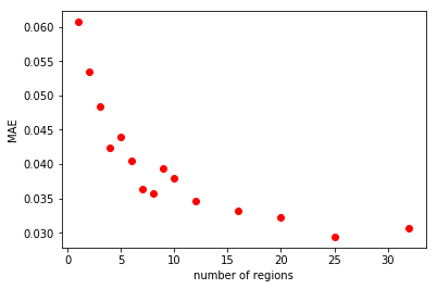
Figure 3. Increasing the number of regions per image decreases the mean absolute error (MAE) of the learned density estimator.

5.3. Synthetic Data (real and integer density)

Using the same methodology, we show that more complex functions can be learned. First, we attempt to learn a function,$f(count)$, with a range of integers as output. Similar to before, we randomly chose colors from the entire CIFAR dataset but this time we selected $20$ random points. For each pixel, we count the total number of the random points that are within a fixed distance ($0.4$) in RGB space. The output is in the range $\left[0,20\right]$. Our approach, RAL, achieves an MAE of $0.267$, compared to an MAE of $0.785$ for the baseline, unif. Sample results are shown in Figure 4 (columns 2–4).

We also tested our method on a real-valued function. We used the same $20$ random points as before and calculated the distances to all points in the dataset. For each pixel, we sorted the $20$ distances and calculated the fraction of the minimum distance divided by the second shortest distance as our density function, $f(ratio)$. For this synthetic function, the MAEs are $0.038$ and $0.176$ for RAL and unif respectively. See Figure 4 (columns 5–7) for example results.

$I$	$f(count)$	$\hat{f}$ (unif)	$\hat{f}$ (RAL)	$f(ratio)$	$\hat{f}$ (unif)	$\hat{f}$ (RAL)

Figure 4. Results for more synthetic functions. For images $I$, we demonstrate our method on two different ground-truth geospatial functions. (column 2) Shows the ground truth for an integer counting function, $f(count)$, with the learned results in columns 3–4. (column 5) Shows the ground truth for a real valued ratio function, $f(ratio)$, with the learned results in columns 6–7.

5.4. Synthetic Data with Priors

In the previous experiments, we only made the assumption that the geospatial density function, $f$, was non-negative, hence the use of the softplus activation on the output layer. In some applications, we may know additional information about the form of the density, such as that it has an upper bound or that it is sparse. In this section, we investigate whether incorporating these priors into the network architecture is beneficial.

We define a new synthetic geospatial density function $f$. Our goal is for this function to be sparse and for the output range to be known (once again we use $\left[0,1\right]$). To create this function, we bin the color space into 16 bins along each of the 3 dimensions of RGB, resulting in $16^{3}=4096$ total bins. We count the number of unique CIFAR images each color bin appears in, and we also calculate the average number of pixels for each time a color bin appears in an image. We select the color bins that appear in a high number of images (at least $29\,000$), but only appear in, on average, 10 pixels or less per image. This results in 26 color bins. We use these bins to create the sparse density function, $f(sparse)$, where we set pixels in the selected color bins to one, while the remaining pixels are set to zero. See Figure 5 (column 2) for examples of this function. We use the same region generation method as before.

For training, we test two different priors. The first is the effect of using sigmoid vs. softplus activation. Using a sigmoid will force the outputs of our predicted density, $\hat{f}$, to be between $\left[0,1\right]$. The second prior is an $L_{1}$ penalty ($\lambda=1\mathrm{e}{-4}$) on the activations of the CNN before the RAL. The goal of this penalty is to encourage sparsity for $\hat{f}$.

We trained 4 combinations with and without using the two different priors: softplus with no activation penalty, softplus with $L_{1}$ activation penalty, sigmoid with no activation penalty, and sigmoid with $L_{1}$ activation penalty. The resulting MAEs were $0.052$, $0.035$, $0.019$, and $0.012$ respectively. For this experiment, enforcing the activation output between $\left[0,1\right]$ with a sigmoid performed better than the softplus activation. Using an $L_{1}$ activation penalty also improved results for a given activation function. This shows that modifying the network architecture to incorporate priors on the geospatial density function, $f$, is an effective strategy for improving performance of the learned estimator. This is a promising result; this strategy could be especially useful in real-world scenarios when training data is limited.

$I$	$f(sparse)$	$\hat{f}$ $(sp)$	$\hat{f}$ $(sp$, $L_{1})$	$\hat{f}$ $(sig)$	$\hat{f}$ $(sig$, $L_{1})$

Figure 5. Enforcing priors over sparse function improves our estimate of the geospatial distribution function. Here we use a sparse, binary ground-truth geospatial function, $f(sparse)$. Columns 3–6 show the estimated densities for models trained with the following settings: softplus activation $\hat{f}$ $(sp)$, softplus activation and $L_{1}$ activation regularization $\hat{f}$ $(sp$, $L_{1})$, sigmoid activation $\hat{f}$ $(sig)$, sigmoid activation and $L_{1}$ activation regularization $\hat{f}$ $(sig$, $L_{1})$. Observe that the results get progressively better as we incorporate priors that match the ground-truth function.

5.5. Census Data Example: Population and Housing Count

We used our proposed approach, RAL, for the task of high-resolution population density estimation. This task could be useful for a wide variety of applications, including improving estimates of population between the official decennial census, by accounting for land use changes, or estimating the population in regions without a formal census. We compare our method to a baseline approach, unif, that assumes the distribution of densities within a region is uniform. With the unif approach, we minimize a per-pixel loss and, therefore, do not need the region definitions during the optimization process. All other aspects of the model, dataset, and optimization strategy are the same.

Evaluation Dataset

We built a large-scale evaluation dataset with diverse geographic locations. For our aggregated training labels, $F$, we used block-group population and housing counts provided from the 2010 US Census. We used RGB imagery from the Planet “Dove” satellite constellation with a ground sample distance (GSD) of $3m$. Training was performed using images from 11 cities across the following geographic subdivisions: Pacific West, Mountain West, West North Central, West South Central, South Atlantic, and Middle Atlantic. The total area of the training set is approximately $14\,000km^{2}$. Our validation consists of held out tiles from these cities, with a total area of approximately $650km^{2}$. Testing was done on tiles from Dallas and Baltimore, with a total area of approximately $3\,000km^{2}$. There are, on average, $~{}50$ regions per tile and each region has, on average, an area of $20\,000m^{2}$.

Mini-Batch Construction

To construct a mini-batch, we randomly sample six tiles, each is $588\times 588$. For data augmentation, we randomly flip left/right and up/down. To normalize the images, we subtract a channel-wise mean value. We use the census block groups to define a region mask, assigning each a unique integer. If there are more than 100 block groups for a given tile, which can happen in dense urban areas, we randomly sample 100 and assign the remainder to the background class. As ground-truth labels we use the population and housing counts for the corresponding census block groups.

Model Architecture

For all experiments, we use the same base neural network architecture, which uses a U-net architecture (Ronneberger et al., 2015), although any pixel-level segmentation network could be used instead. See Table 1 for details of the layers of this architecture, except the final output layer, which varies depending on the task. The concat layer is a channel-wise concatenation. The up() operation is a $2\times$ up-sampling using nearest neighbor interpolation and the maxpool() operation represents a $2\times 2$ max pooling. All convolutional layers use a $3\times 3$ kernel and each, except the final one, is followed by a batch normalization layer. This network was pre-trained, using standard techniques, for pixel-level classification for several output classes, including roads and buildings.

Table 1. The neural network architecture we use for the census data experiments.

type (name)	inputs	output channels
conv2d (conv1.1)	image	32
conv2d (conv1.2)	conv1.1	32
conv2d (conv2.1)	maxpool(conv1.2)	64
conv2d (conv2.2)	conv2.1	64
conv2d (conv3.1)	maxpool(conv2.2)	128
conv2d (conv3.2)	conv3.1	128
conv2d (conv4.1)	maxpool(conv3.2)	256
conv2d (conv4.2)	conv4.1	256
concat (up5)	up(conv4.2), conv3.2	384
conv2d (conv5.1)	up5	128
conv2d (conv5.2)	conv5.1	128
concat (up6)	up(conv5.2), conv2.2	192
conv2d (conv6.1)	up6	64
conv2d (conv6.2)	conv6.1	64
concat (up7)	up(conv6.2), conv1.2	96
conv2d (conv7.1)	up7	32
conv2d (conv7.2)	conv7.1	32

	$R$	$\hat{f}_{pop}$ (RAL)	$\hat{f}_{house}$ (RAL)	bldg. class

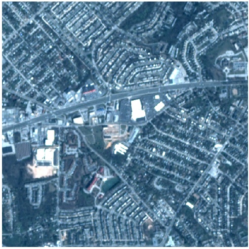
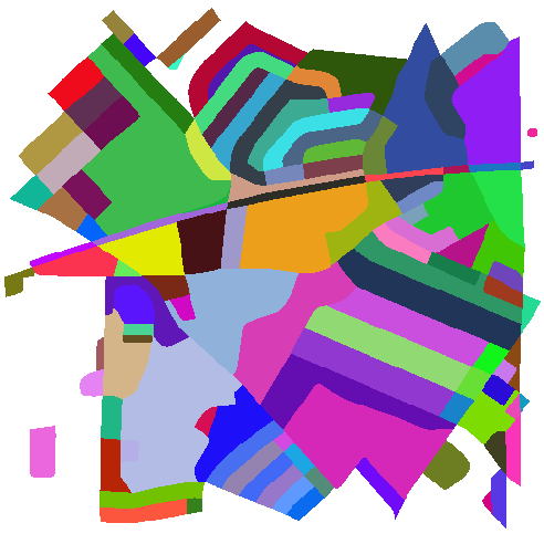
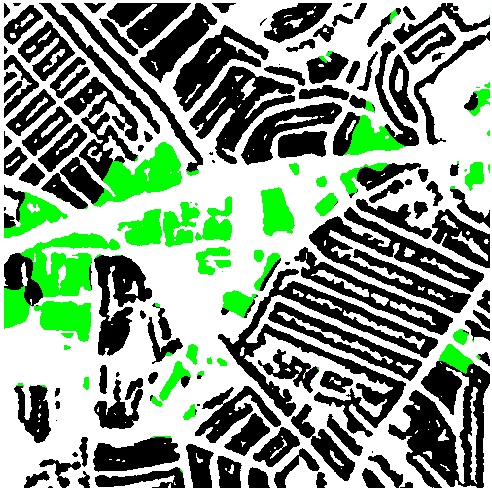
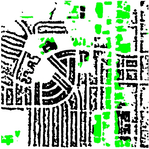
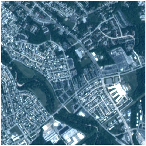
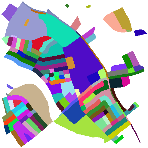
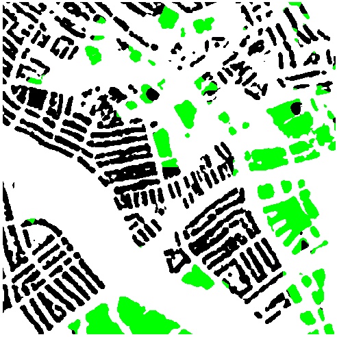
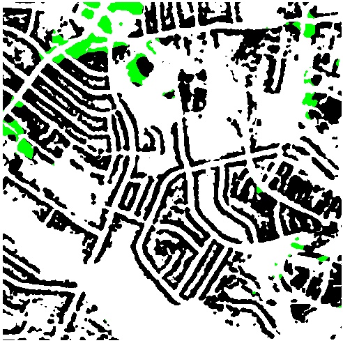
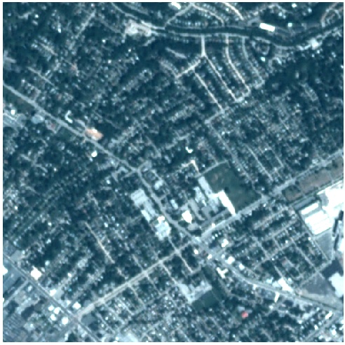
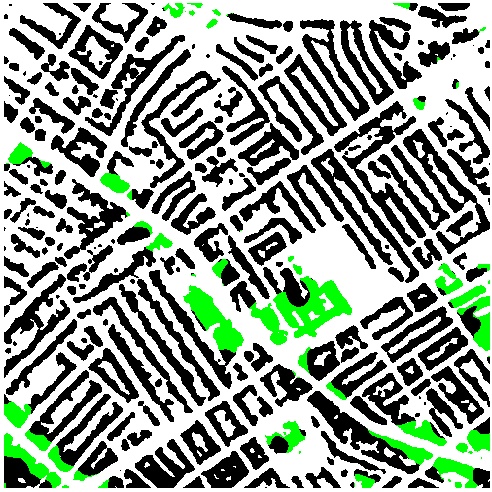
Figure 6. Visualizations of various outputs of our model for different scenes. From left to right: the input image; the census block groups (white pixels correspond to regions that are not fully contained in the image); raw per-pixel density estimates for population and housing; and our building type classification.

We add two $1\times 1$ convolution layers to the base network to represent the per-pixel densities, one for population and one for housing count. Each takes as input the logits of the base network and has a softplus activation function. During training, the output of these final layers are passed to a regional aggregation layer (RAL) to generate the aggregated sums. During inference, we remove the RAL and our network outputs the per-pixel densities for both object classes.

Model Fitting

We trained our model using the AMSGrad (Reddi et al., 2018) optimizer, a variant of the Adam (Kingma and Ba, 2014) optimizer, with a weight decay of $5\mathrm{e}{-4}$. The initial learning rate was set to $0.001$ and we reduced the learning rate by a factor of $0.5$ every $2\,000$ iterations. We trained for $20\,000$ iterations, but only keep the best checkpoint, based on validation accuracy.

Results

We first show qualitative output from our model. Figure 6 shows the population and housing density estimates for a satellite image. We also show the use of these estimates to do rough disambiguation between residential and non-residential buildings. To accomplish this, we first applied a pre-trained building segmentation CNN and thresholded it at $0.2$. We applied a Gaussian blur ($\sigma=4$) to our estimated house density and thresholded at $0.001$. We then constructed a false color image where white pixels are background, black pixels correspond to buildings that we detected with a house density above the threshold (residential), and green pixels correspond to buildings with a house density below the threshold (non-residential).

	$\hat{f}_{pop}$ (unif)	$\hat{f}_{pop}$ (RAL)

Figure 7. A comparison of two training methods for the task of population density estimation: uniformly distributing the aggregated sum (middle) and our method (right).

For quantitative evaluation, since we don’t know the true per-pixel densities, we evaluate using the aggregated estimates on the held-out cities. We use the pixel-level outputs from our models and accumulate the densities for each region independently. We find that the uniform baseline method, unif, has an MAE of 27.7 for population count and 12.1 for housing density. In comparison, our method, RAL, has MAEs of 26.5 and 11.7 respectively. While these methods are fairly close in terms of MAE, the pixel-level densities estimated by both training strategies are very different. Figure 7 compares these density maps. This shows that our approach more clearly delineates the locations of residential dwellings, which makes this potentially more useful for integration with different applications.

Dasymetric Mapping

While our method does not require known aggregated sums at inference time, it is straightforward to use them if they are given. Figure 8 shows the result of applying dasymetric mapping using our pixel-level population and housing density predictions as a guide for redistributing the ground-truth aggregated sums. It is difficult to evaluate the effectiveness of this approach, since high-resolution density estimates are not available. However, this approach is promising because the learned CNN is trained in an end-to-end manner and, hence, does not require any special knowledge of the input imagery or assumptions about the distribution of objects.

	$R$	$\hat{f}_{pop}$ (RAL)	$\hat{f}_{pop}$ (dasy)	$\hat{f}_{house}$ (RAL)	$\hat{f}_{house}$ (dasy)

Figure 8. Examples of using our model as a distribution estimate for dasymetric mapping. From left to right: the input image; the census block groups (white pixels correspond to regions that are not fully contained in the image); per-pixel density estimates for population and housing, both raw and dasymetric (note that the dasymetric mapping sets population densities to zero for regions outside the image).

Discussion

One of the key limitations with our evaluation is that the Census data provides an estimate for the state of the country in 2010, but our imagery is from 2015–2017. This could lead to a variety of errors, for example replacing a residential neighborhood with a commercial district, constructing a new neighborhood on farm land, or changing the housing density by infill construction. It may be possible to address these problem by making assumptions on the expected frequency of various types of change, but the best solution is likely to wait for the results of the next Census and capture imagery at roughly the same time.

6. Conclusions

We proposed an approach for learning to estimate pixel-level density functions from high-resolution satellite imagery when only coarse-grained density aggregates are available for training. Our approach can be used in conjunction with any pixel-level labeling CNN using standard deep learning libraries.

We showed that this technique works well on a variety of synthetic datasets and for a large real-world dataset. The main innovation is incorporating a layer that replicates the regional aggregation process in the network in a way that enables end-to-end network optimization. Since this layer is not required to estimate the pixel-level density, we can remove it at inference time. The end result is a CNN that estimates the density with significantly higher effective resolution than the baseline approach. We also showed that when additional information is available about the form of the density function, we can constrain the learning process, using custom activation functions or activity regularization, to improve our ability to learn with fewer samples.

One limitation of our current implementation is that it requires a region to be fully contained in an input image because it computes the region aggregation in a single forward pass. When regions are large and the image resolution is high it may not be possible to do this due to memory constraints. One way to overcome this would be to partition the image and compute the aggregation over multiple forward passes. It would then be straightforward to compute the backward pass separately for each sub-image.

For future work, we intend to apply this technique to a variety of different geospatial density mapping problems, explore additional ways of incorporating priors, and investigate extensions to structured density estimation.

References

- (1)
- Bargiel (2017) Damian Bargiel. 2017. A new method for crop classification combining time series of radar images and crop phenology information. Remote Sensing of Environment (2017).
- Chattopadhyay et al. (2017) P. Chattopadhyay, R. Vedantam, R. R. Selvaraju, D. Batra, and D. Parikh. 2017. Counting Everyday Objects in Everyday Scenes. In CVPR.
- Chen et al. (2018a) Liang-Chieh Chen, Alexander Hermans, George Papandreou, Florian Schroff, Peng Wang, and Hartwig Adam. 2018a. MaskLab: Instance Segmentation by Refining Object Detection with Semantic and Direction Features. In CVPR.
- Chen et al. (2018b) Liang-Chieh Chen, Yukun Zhu, George Papandreou, Florian Schroff, and Hartwig Adam. 2018b. Encoder-Decoder with Atrous Separable Convolution for Semantic Image Segmentation. In ECCV.
- Dobson et al. (2000) Jerome E Dobson, Edward A Bright, Phillip R Coleman, Richard C Durfee, and Brian A Worley. 2000. LandScan: a global population database for estimating populations at risk. Photogrammetric engineering and remote sensing (2000).
- Doupe et al. (2016) Patrick Doupe, Emilie Bruzelius, James Faghmous, and Samuel G Ruchman. 2016. Equitable development through deep learning: The case of sub-national population density estimation. In ACM Annual Symposium on Computing for Development.
- Dugas et al. (2001) Charles Dugas, Yoshua Bengio, François Bélisle, Claude Nadeau, and René Garcia. 2001. Incorporating second-order functional knowledge for better option pricing. In Advances in Neural Information Processing Systems.
- Eicher and Brewer (2001) Cory L Eicher and Cynthia A Brewer. 2001. Dasymetric mapping and areal interpolation: Implementation and evaluation. Cartography and Geographic Information Science (2001).
- Facebook Connectivity Lab and Center for International Earth Science Information Network, Columbia University (2016) Facebook Connectivity Lab and Center for International Earth Science Information Network, Columbia University. 2016. High Resolution Settlement Layer. https://www.ciesin.columbia.edu/data/hrsl/ [Online; accessed 5-Sep-2018].
- Fisher and Langford (1996) Peter F Fisher and Mitchel Langford. 1996. Modeling sensitivity to accuracy in classified imagery: A study of areal interpolation by dasymetric mapping. The Professional Geographer (1996).
- Gao et al. (2018) Mingfei Gao, Ang Li, Ruichi Yu, Vlad I Morariu, and Larry S Davis. 2018. C-WSL: Count-guided Weakly Supervised Localization. In ECCV.
- Gaughan et al. (2015) AE Gaughan, Forrest R Stevens, Catherine Linard, Nirav N Patel, and Andrew J Tatem. 2015. Exploring nationally and regionally defined models for large area population mapping. International Journal of Digital Earth (2015).
- He et al. (2017) Kaiming He, Georgia Gkioxari, Piotr Dollár, and Ross Girshick. 2017. Mask R-CNN. In ICCV.
- Holt et al. (2004) James B Holt, CP Lo, and Thomas W Hodler. 2004. Dasymetric estimation of population density and areal interpolation of census data. Cartography and Geographic Information Science (2004).
- Ji et al. (2018) Shunping Ji, Chi Zhang, Anjian Xu, Yun Shi, and Yulin Duan. 2018. 3D Convolutional Neural Networks for Crop Classification with Multi-Temporal Remote Sensing Images. Remote Sensing (2018).
- Khoreva et al. (2017) Anna Khoreva, Rodrigo Benenson, Jan Hosang, Matthias Hein, and Bernt Schiele. 2017. Simple does it: Weakly supervised instance and semantic segmentation. In CVPR.
- Kingma and Ba (2014) Diederik P Kingma and Jimmy Ba. 2014. Adam: A method for stochastic optimization. arXiv preprint arXiv:1412.6980 (2014).
- Krizhevsky (2009) Alex Krizhevsky. 2009. Learning multiple layers of features from tiny images. Technical Report. University of Toronto.
- Krizhevsky et al. (2012) Alex Krizhevsky, Ilya Sutskever, and Geoffrey E Hinton. 2012. Imagenet classification with deep convolutional neural networks. In Advances in Neural Information Processing Systems.
- Kussul et al. (2017a) Nataliia Kussul, Andrii Kolotii, Andrii Shelestov, Bohdan Yailymov, and Mykola Lavreniuk. 2017a. Land degradation estimation from global and national satellite based datasets within UN program. In IEEE International Conference on Intelligent Data Acquisition and Advanced Computing Systems: Technology and Applications.
- Kussul et al. (2017b) Nataliia Kussul, Mykola Lavreniuk, Sergii Skakun, and Andrii Shelestov. 2017b. Deep learning classification of land cover and crop types using remote sensing data. IEEE Geoscience and Remote Sensing Letters (2017).
- Langford and Unwin (1994) Mitchel Langford and David J Unwin. 1994. Generating and mapping population density surfaces within a geographical information system. The Cartographic Journal (1994).
- Lin et al. (2013) Min Lin, Qiang Chen, and Shuicheng Yan. 2013. Network in network. arXiv preprint arXiv:1312.4400 (2013).
- Mennis (2003) Jeremy Mennis. 2003. Generating surface models of population using dasymetric mapping. The Professional Geographer (2003).
- Onoro-Rubio and López-Sastre (2016) Daniel Onoro-Rubio and Roberto J López-Sastre. 2016. Towards perspective-free object counting with deep learning. In ECCV.
- Pascual et al. (2018) Guillem Pascual, Santi Seguí, and Jordi Vitrià. 2018. Uncertainty Gated Network for Land Cover Segmentation. In DeepGlobe (IEEE CVPR Workshop).
- Pavía and Cantarino (2017) Jose M Pavía and Isidro Cantarino. 2017. Can dasymetric mapping significantly improve population data reallocation in a dense urban area? Geographical Analysis (2017).
- Peng et al. (2017) Chao Peng, Xiangyu Zhang, Gang Yu, Guiming Luo, and Jian Sun. 2017. Large Kernel Matters–Improve Semantic Segmentation by Global Convolutional Network. In CVPR.
- Pomente and Aleandri (2017) Andrea Pomente and David Aleandri. 2017. Convolutional expectation maximization for population estimation. CLEF working notes, CEUR.
- Reddi et al. (2018) Sashank J Reddi, Satyen Kale, and Sanjiv Kumar. 2018. On the convergence of adam and beyond. In International Conference on Learning Representations.
- Redmon and Farhadi (2017) Joseph Redmon and Ali Farhadi. 2017. YOLO9000: Better, Faster, Stronger. In CVPR.
- Robinson et al. (2017) Caleb Robinson, Fred Hohman, and Bistra Dilkina. 2017. A Deep Learning Approach for Population Estimation from Satellite Imagery. In ACM SIGSPATIAL Workshop on Geospatial Humanities.
- Ronneberger et al. (2015) Olaf Ronneberger, Philipp Fischer, and Thomas Brox. 2015. U-net: Convolutional networks for biomedical image segmentation. In MICCAI.
- Russakovsky et al. (2015) Olga Russakovsky, Jia Deng, Hao Su, Jonathan Krause, Sanjeev Satheesh, Sean Ma, Zhiheng Huang, Andrej Karpathy, Aditya Khosla, Michael Bernstein, Alexander C. Berg, and Li Fei-Fei. 2015. ImageNet Large Scale Visual Recognition Challenge. International Journal of Computer Vision (2015).
- Simonyan and Zisserman (2014) Karen Simonyan and Andrew Zisserman. 2014. Very deep convolutional networks for large-scale image recognition. arXiv preprint arXiv:1409.1556 (2014).
- Sindagi and Patel (2017) Vishwanath A Sindagi and Vishal M Patel. 2017. Generating high-quality crowd density maps using contextual pyramid CNNs. In ICCV.
- Sorichetta et al. (2015) Alessandro Sorichetta, Graeme M Hornby, Forrest R Stevens, Andrea E Gaughan, Catherine Linard, and Andrew J Tatem. 2015. High-resolution gridded population datasets for Latin America and the Caribbean in 2010, 2015, and 2020. Scientific Data (2015).
- Stevens et al. (2015) Forrest R Stevens, Andrea E Gaughan, Catherine Linard, and Andrew J Tatem. 2015. Disaggregating census data for population mapping using random forests with remotely-sensed and ancillary data. PLOS ONE (2015).
- Wright (1936) John K Wright. 1936. A method of mapping densities of population: With Cape Cod as an example. Geographical Review (1936).
- Zhang et al. (2015) Jianming Zhang, Shugao Ma, Mehrnoosh Sameki, Stan Sclaroff, Margrit Betke, Zhe Lin, Xiaohui Shen, Brian Price, and Radomir Mech. 2015. Salient object subitizing. In CVPR.
- Zhao et al. (2017) Hengshuang Zhao, Jianping Shi, Xiaojuan Qi, Xiaogang Wang, and Jiaya Jia. 2017. Pyramid Scene Parsing Network. In CVPR.
- Zhou et al. (2016) Bolei Zhou, Aditya Khosla, Agata Lapedriza, Aude Oliva, and Antonio Torralba. 2016. Learning deep features for discriminative localization. In CVPR.
- Zhou et al. (2018) Yanzhao Zhou, Yi Zhu, Qixiang Ye, Qiang Qiu, and Jianbin Jiao. 2018. Weakly Supervised Instance Segmentation using Class Peak Response. In CVPR.
- Zoph et al. (2018) Barret Zoph, Vijay Vasudevan, Jonathon Shlens, and Quoc V Le. 2018. Learning Transferable Architectures for Scalable Image Recognition. In CVPR.