Mixed WIMP-axion dark matter

Abstract

We study the experimental constraints on a model of a two-component dark matter, consisting of the QCD axion, and a scalar particle, both contributing to the dark matter relic abundance of the Universe. The global Peccei-Quinn symmetry of the theory can be spontaneously broken down to a residual $\mathbb{Z}_{2}$ symmetry, thereby identifying this scalar as a stable weakly interacting massive particle, i.e., a dark matter candidate, in addition to the axion. We perform a comprehensive study of the model using the latest data from dark matter direct and indirect detection experiments, as well as new physics searches at the Large Hadron Collider. We find that although the model is mostly constrained by the dark matter detection experiments, it is still viable around a small region of the parameter space where the scalar dark matter is half as heavy as the Standard Model Higgs. In this allowed region, the bounds from these experiments are evaded due to a cancellation mechanism in the dark matter–Higgs coupling. The collider search results, however, are shown to impose weak bounds on the model.

I Introduction

The evidence of cold dark matter (CDM) is overwhelming from the cosmological data, even though its detection and identification continue to be one of the most interesting and challenging problems today [1]. Many particle dark matter (DM) models have been proposed over the last few decades, one of the oldest of them being the weakly interacting massive particle (WIMP) model [2, 3, 4, 5] (for reviews, see [6, 7, 8]). In the WIMP scenario, the dark matter relic abundance is obtained through the annihilation of dark matter particles in the early Universe with weak scale cross sections and electroweak scale masses [2, 9, 10, 11]. The fact that one gets new physics at the electroweak scale for a WIMP mass $\sim\!100{\rm\ GeV}$ makes this scenario a very appealing solution to the dark matter problem [12].

The absence of $CP$ violation in the strong sector of the Standard Model (SM) is another long-standing puzzle in the particle physics community [13]. The null results of the neutron electric dipole moment measurement experiments so far restrict the value of the coefficient $\theta_{\rm QCD}$ of the parity-violating $\mathbf{E}\cdot\mathbf{B}$ operator to be less than $10^{-10}$ [14]. In the present form of the SM, this is a fine-tuning problem since there is no symmetry that protects such a small number from large higher-order corrections [15]. Therefore, a natural explanation of the smallness of strong $CP$ violation is sought, and an elegant solution to this puzzle is given by the introduction of a global $U(1)$ Peccei-Quinn (PQ) symmetry [16, 17, 18, 19, 20]. This symmetry is spontaneously broken at a scale much larger than the electroweak scale by a scalar field, with the axion as the corresponding massless Nambu-Goldstone boson of this $U(1)_{\rm PQ}$ symmetry. The coefficient $\theta_{\rm QCD}$ is dynamic in this model and its small value is naturally attained in this way and is inversely proportional to the PQ scale. In this context, a large number of axion models have been proposed in the literature. The early PQ model, first proposed in [16] and further developed in [17, 18], augments the SM with an additional complex scalar, charged under the electroweak (EW) symmetry. The Lagrangian is additionally invariant under a global $U(1)$ symmetry, which is spontaneously broken at the EW scale. However, this model predicts large axion couplings and hence is ruled out by experiments [21]. To circumvent the experimental bounds, invisible axion models were proposed independently: the Kim-Shifman-Vainshtein-Zakharov (KSVZ) model [19, 20] and the Dine-Fischler-Srednicki-Zhitnitsky (DFSZ) [22, 23] model. The KSVZ model introduces heavy, colored, EW singlet quarks, in addition to the PQ scalar. In this model, the axions have no direct tree-level couplings with the SM fields and can only have induced couplings to the SM leptons. On the other hand, the DFSZ model introduces an additional Higgs field, along with the PQ scalar. This allows the axions to have natural couplings to leptons at tree level. Other than this, axionlike Goldstone particles arise in a multitude of other theoretical scenarios as well, e.g., majorons [24, 25], familons [26, 27, 28], axions from string theory [29, 30, 31], axions from accidental symmetry breaking [32, 33, 34], etc.

The axion field gains a small mass inversely proportional to the $U(1)_{\rm PQ}$-breaking scale, after the QCD condensation at a temperature of about $T\simeq 200$ MeV. In the early Universe, the axion can be produced nonrelativistically through a coherent oscillation of the axion field due to the misalignment of the PQ vacuum. This is known as the misalignment mechanism of axion production [35, 36]. The axion is not completely stable; however, it has very feeble couplings with SM particles, thereby ensuring a lifetime longer than the age of the Universe [37]. This makes the axion a very good CDM candidate [38, 39, 40], although the same feeble couplings make direct detection of these axions challenging [39].

Since current DM detection experiments have shown null results, one needs to look for other alternatives to the simple WIMP scenario. One such alternative is a multicomponent DM, where one component acts as a WIMP, whereas the other components might have very different interactions. These models are less constrained due to the fact that the fraction of WIMPs in these multicomponent DM has not been determined experimentally and hence is a free parameter. This has been shown to have interesting phenomenological consequences [41, 42, 43, 44, 45, 46, 47, 48].

In this work, we study a two-component DM model consisting of a WIMP and the axion as the DM candidates. This type of model gives a unifying scenario where the PQ field, which is motivated to solve the strong-$CP$ problem, and the WIMP, which is a natural solution to DM puzzle, can be accommodated in a single go [49, 46]. Furthermore, these models can also be extended to include neutrino masses [49]. Hence, these models, and their variations thereof, can account for three of the most important puzzles in the SM. Possible UV completions are considered in [46]. As a simple realization of this, one can consider the KSVZ model of axion with an additional scalar field charged under the $U(1)_{\rm PQ}$ [49]. This additional scalar gets its stability from the residual $\mathbb{Z}_{2}$ symmetry of the broken $U(1)_{\rm PQ}$ and hence becomes a WIMP-like DM candidate [50]. Breaking of the $U(1)_{\rm PQ}$ and the electroweak symmetry leads to a mixing between the Higgs and the radial part of the PQ scalar, which leads to interesting phenomenological consequences. The advantage of this model is that although the axions have very weak interactions with the SM, the coupling between this dark scalar and the SM Higgs doublet provides a portal to test this model in different DM detection experiments, both direct and indirect. The model can also give different signatures at collider experiments. For example, the KSVZ model predicts new colored, electroweak singlet quarks, which can be produced at colliders. Mixing with a scalar affects the properties of the Higgs boson, which can be directly used to constrain the mixing parameters. Furthermore, the dark scalar can also contribute to momentum imbalance in a collision event.

Hence, in the light of recent experiments, we explore the constraints on the WIMP-axion DM model, both from DM search experiments as well as collider searches. Using the latest limit on DM-nucleon scattering cross section from XENON1T$\times$1 yr experiment data [51], we find that the phenomenologically interesting mass range of $m_{\rm DM}\gtrsim 100{\rm\ GeV}$ is ruled out in such models. However, the stringent bounds from XENON1T$\times$1 yr data can be evaded in a small region of the parameter space where the scalar dark matter is half as heavy as the Higgs. This is a direct outcome of the mixing of the Higgs with the scalar, which leads to a cancellation mechanism in the Higgs portal coupling, thereby reducing the DM-nucleon scattering cross section. As a result, while minimal scalar DM models are mostly ruled out by direct detection bounds [52], such WIMP-axion models can still survive with a reduced parameter space. Collider signals, on the other hand, are highly plagued by the backgrounds from the production of Standard Model particles, and hence the signals are not significant enough to be observed above the background [53, 54, 55].

The paper is organized as follows. Section II discusses the model and the different parameters involved. Section III talks about the different experimental bounds, and how they constrain the parameters of the model. In Sec. IV, we summarize the main results, and finally in Sec. V, we conclude.

II The Model

We consider the KSVZ model of the axion, where electroweak singlet quarks $Q_{L}$ and $Q_{R}$ and a complex scalar $\zeta$, both transforming under a global $U(1)_{\rm PQ}$ symmetry, are added to the SM [19, 20]. These quarks are vectorlike and hence do not introduce any chiral anomaly [56, 57]. We augment this model with a complex scalar $\chi\!=\!(\chi_{1}+i\chi_{2})/\sqrt{2}$ which is a SM singlet but charged under the $U(1)_{\rm PQ}$ symmetry [49]. The axion $a$ is the Nambu-Goldstone mode of the scalar field $\zeta$, which can couple to the vectorlike quarks as well as $\chi$. As in the original KSVZ model, the axion can act as a CDM candidate [39]. The charges and quantum numbers of the new particles are listed in Table 1.

Table 1: New particles in the model and their charges. PQ charges of all the SM particles are zero.

	$\zeta$	$\chi$	$Q_{L}$	$Q_{R}$
Spin	0	0	1/2	1/2
$SU(3)_{C}$	1	1	3	3
$SU(2)_{L}$	1	1	1	1
$U(1)_{Y}$	0	0	$-1/3$	$-1/3$
$U(1)_{PQ}$	2	1	1	$-1$

The relevant part of the Lagrangian, governing the interactions of $Q_{L,R},\,\zeta$, and $\chi$ with the SM, is given by

$$\mathcal{L} \supset -\lambda_{H}\left(|H|^{2}-\frac{v_{H}^{2}}{2}\right)^{2}-\lambda_{\zeta}\left(\left|\zeta\right|^{2}-\frac{F_{a}^{2}}{2}\right)^{2}$$ (1)

$$-\lambda_{\zeta H}\left(\left|H\right|^{2}-\frac{v_{H}^{2}}{2}\right)\left(\left|\zeta\right|^{2}-\frac{F_{a}^{2}}{2}\right)-\lambda_{\chi}\left|\chi\right|^{4}$$

$$-\mu_{\chi}^{2}\left|\chi\right|^{2}-\lambda_{\chi H}\left|H\right|^{2}\left|\chi\right|^{2}-\lambda_{\zeta\chi}\left|\zeta\right|^{2}\left|\chi\right|^{2}$$

$$+\Big{[}\epsilon_{\chi}\zeta^{*}\chi^{2}+f_{d}\chi\bar{Q}_{L}d_{R}+f_{Q}\zeta\bar{Q}_{L}Q_{R}+\text{H.c.}\Big{]}\,.$$

Here $H$ is the SM Higgs doublet and $d_{R}$ represents right-handed down-type quarks in the SM. After electroweak symmetry breaking via the Higgs vacuum expectation value (VEV) $v_{H}$, one has $|H|=(h_{0}+v_{H})/\sqrt{2}$, where $h_{0}$ is the Higgs boson. Similarly, using the nonlinear representation, one can write $\zeta=e^{ia\,/F_{a}}\left(F_{a}+\sigma_{0}\right)/\sqrt{2}$, where $F_{a}$ is the $U(1)_{\rm PQ}$-symmetry-breaking scale, also known as the axion decay constant, and $\sigma_{0}$ is the radial excitation of the $\zeta$ field. Constraints from supernova cooling data disfavor values of $F_{a}$ smaller than $10^{10}{\rm\ GeV}$ [58].

After the breaking of both the symmetries, viz. electroweak and PQ symmetries, the interaction term between $H$ and $\zeta$ fields leads to mixing between $h_{0}$ and $\sigma_{0}$ with the mass matrix

$$M^{2}\equiv\begin{pmatrix}2v_{H}^{2}\lambda_{H}&&F_{a}v_{H}\lambda_{\zeta H}\\ F_{a}v_{H}\lambda_{\zeta H}&&2F_{a}^{2}\lambda_{\zeta}\\ \end{pmatrix}.$$ (2)

As a result of the mixing, the scalars in the mass basis are related to those in the flavor basis as

$$\begin{pmatrix}h\\ \sigma\end{pmatrix}=\begin{pmatrix}\cos\,\theta&&-\sin\,\theta\\ \sin\,\theta&&\cos\,\theta\\ \end{pmatrix}\begin{pmatrix}h_{0}\\ \sigma_{0}\end{pmatrix},$$ (3)

where the mixing angle, in the limit $F_{a}\gg v_{H}$, is given by

$$\sin\,\theta\simeq\frac{v_{H}}{F_{a}}\frac{\lambda_{\zeta H}}{2\lambda_{\zeta}}.$$ (4)

One obtains the masses of the physical states as

$$m_{h} \simeq \,v_{H}\sqrt{2\lambda_{H}\left(1-\frac{\lambda_{\zeta H}^{2}}{4\lambda_{H}\lambda_{\zeta}}\right)}\,+\mathcal{O}\left(\frac{v_{H}}{F_{a}}\right),$$ (5)

$$m_{\sigma} \simeq \,F_{a}\sqrt{2\lambda_{\zeta}}+\mathcal{O}\left(\frac{v_{H}}{F_{a}}\right).$$ (6)

Note that the mass $m_{h}$ of the mixed state $h$ is no longer $\sqrt{2\lambda_{H}v_{H}^{2}}$, as predicted by the SM. Since $h$ is the physical state, we fix $m_{h}$ at $125$ GeV and the Higgs VEV $v_{H}$ at $246$ GeV to match with the experimentally measured masses of the observed scalar [59, 60] and $W$ and $Z$ bosons, respectively [61]. The value of $\lambda_{H}$ is no longer the SM value, $\lambda^{\text{SM}}_{H}\simeq 0.13$, but is dependent on other parameters in this model and can be calculated using Eq. (5). In fact, if we take $\lambda_{H}=\lambda_{H}^{\text{SM}}=\frac{m_{h}^{2}}{2v_{H}^{2}}$, from Eq. (5) it is evident that $\lambda_{\zeta H}$ has to be zero; i.e., the SM Higgs does not mix with $\zeta$, as considered in [49]. Note that there is no underlying symmetry in the theory that allows us to set $\lambda_{\zeta H}$ to zero in the Lagrangian. More importantly, although the mixing is very small, the relation between the masses of the physical states with other model parameters plays a major role in imposing constraints on the model. Therefore, we do not neglect the mixing of $h_{0}$ with $\sigma_{0}$ in this study.

The masses of $\chi_{1}$ and $\chi_{2}$ are given by

$$m_{\chi_{1,2}}^{2}=\frac{1}{2}\left(2\mu_{\chi}^{2}+v_{H}^{2}\lambda_{\chi H}+F_{a}^{2}\lambda_{\zeta\chi}\mp 2\sqrt{2}F_{a}\epsilon_{\chi}\right).$$ (7)

Without loss of generality, we can take $\epsilon_{\chi}\!>0$ such that $m_{\chi_{1}}\!<m_{\chi_{2}}$; hence $\chi_{1}$ can be the DM candidate, and we, henceforth, denote the mass of $\chi_{1}$ as just $m_{\chi}$. Note that after the PQ-symmetry breaking, the Lagrangian in Eq. (1) has a residual $\mathbb{Z}_{2}$ symmetry which stabilizes $\chi_{1}$. It should also be noted that in Eq. (7), $\mu_{\chi}^{2}$ is defined to be negative and hence cancels out the large contribution coming from $F_{a}$. This type of fine-tuning is a general feature of these axion models [62, 63, 64, 65, 49]. Since the fine-tuning is required mainly in the dark sector, we do not explore it further and defer the details to a later work. Furthermore, one can also motivate a tiny value of $\epsilon_{\chi}$ from naturalness arguments. As $\epsilon_{\chi}\rightarrow 0$, one obtains an extra $U(1)$ symmetry in the theory, apart from the $U(1)_{\rm PQ}$. This can allow $\epsilon_{\chi}$ to be naturally small. Note that a small $\epsilon_{\chi}$ does not necessarily mean a small mass split between the two DM states. For example, we shall consider values around $F_{a}\sim 10^{10}$ GeV, which means the mass split is $\Delta_{\chi}\simeq\sqrt{F_{a}\epsilon_{\chi}}\sim 1{\rm\ TeV}$. This is much larger than the mass of the lighter state.

At this point, it is important to note that in this setup the complex scalar $\chi$ can, in principle, develop a VEV before the PQ field $\zeta$. This can be prevented if parameters are tuned such that the VEV of $\chi$, $v_{\chi}=\sqrt{-\left(\mu_{\chi}^{2}/2\lambda_{\chi}\right)}$, remains smaller than that of $\zeta$. It is always possible to tune $\epsilon_{\chi}$ and $\mu_{\chi}$ such that the mass of $\chi_{1}$ remains fixed, and $v_{\chi}$ remains below $F_{a}$. This is because the only place where $\mu_{\chi}$ and $F_{a}$ appear is in the expression for the masses of the real scalars in Eq. (7). Since the mass difference between $\chi_{1}$ and $\chi_{2}$ is proportional to $\epsilon_{\chi}$, this has the effect of changing the mass of the heavier scalar $\chi_{2}$. However, in our analysis, $\chi_{2}$ is heavy enough to be decoupled from the particle content. With this setup, one can ensure that at a very high scale, around $F_{a}$, breaking of the PQ symmetry occurs before the symmetry breaking of $\chi$. After the PQ-symmetry breaking, $\chi_{1}$ and $\chi_{2}$ may or may not remain tachyonic depending on the choice of parameters. However, we have to ensure that none of them can develop a VEV earlier than the electroweak scale in order to make our mechanism work. Once the Higgs develops a VEV, both $\chi_{1}$ and $\chi_{2}$ become nontachyonic, irrespective of whether they were tachyonic or not prior to the electroweak symmetry breaking. The details of this mechanism is worked out in the Appendix.

The mass of the axion is generated through nonperturbative QCD effects and is inversely proportional to $F_{a}$ [66];

$$m_{a}\simeq 0.6\,{\rm meV}\,\times\left(\frac{10^{10}\,{\rm GeV}}{F_{a}}\right).$$ (8)

The couplings of the axion to SM particles are also suppressed by inverse power of $F_{a}$, so the decay lifetime of the axion is very large. In fact, if we take the value of $F_{a}>10^{10}$ GeV, as allowed by the supernova cooling data [58], its lifetime becomes larger than the age of the Universe. Thus, the axion also acts as a viable candidate for CDM in this model. Therefore, both $\chi_{1}$ and the axion will contribute to the total DM relic density in the Universe.

Finally, the vectorlike quarks obtain their mass $m_{Q}=f_{Q}F_{a}/\sqrt{2}$ after $\zeta$ develops a VEV. If this mass is $\sim\mathcal{O}({\rm TeV})$, they can be produced at the LHC. This is expected to give direct constraints on this model; however, in order to have a mass of $\sim\mathcal{O}({\rm TeV})$, the coupling $f_{Q}$ needs to be extremely tiny $\sim\mathcal{O}(10^{-6})$.

The new interactions introduce two portals connecting the SM and the dark sector through the Higgs (via the $h\chi_{1}\chi_{1}$) and the down-type quark (via the $\chi_{1}\bar{Q}_{L}d_{R}$). Of the two, the $h\chi_{1}\chi_{1}$ interaction is the more important one and will play a key role in our analysis. The $h\chi_{1}\chi_{1}$ coupling is given by

$$g_{h\chi_{1}\chi_{1}}=i\left(F_{a}\lambda_{\zeta\chi}\sin\theta-v_{H}\lambda_{\chi H}\cos\theta-\sqrt{2}\epsilon_{\chi}\sin\theta\right).$$ (9)

Although $\sin\theta$ is small, the first term cannot be ignored due to the large scale $F_{a}$. Using the approximation for $\sin\theta$ in Eq. (4), we obtain

$$g_{h\chi_{1}\chi_{1}}\simeq i\,v_{H}\left(\frac{\lambda_{\zeta\chi}\lambda_{\zeta H}}{2\lambda_{\zeta}}-\lambda_{\chi H}\right).$$ (10)

Note that in the presence of nonzero $\lambda_{\zeta H}$, the $h\chi_{1}\chi_{1}$ coupling vanishes at

$$\lambda_{\chi H}=\frac{\lambda_{\zeta\chi}\lambda_{\zeta H}}{2\lambda_{\zeta}}\,.$$ (11)

This is where we differ from [49], where the authors had set $\lambda_{\zeta H}=0$, which led to the vanishing of the $h\chi_{1}\chi_{1}$ coupling at $\lambda_{\chi H}=0$ . This shift will play a crucial role in the following analysis.

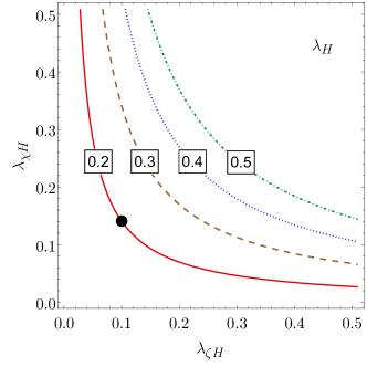
Figure 1: Contours of $\lambda_{H}$, for which the $h\chi_{1}\chi_{1}$ coupling vanishes. The other parameters considered are $\lambda_{\zeta\chi}=0.1,\,v_{H}=246\,{\rm GeV}$ and $m_{h}=125{\rm\ GeV}$. The benchmark point chosen for further analysis, $\lambda_{\zeta H}=0.1,\,\lambda_{\chi H}=0.14$, and $\lambda_{H}=0.2$, is shown as a black circle.

Using Eq. (5), $\lambda_{\zeta}$ can be written in terms of $m_{h},\,\lambda_{\zeta H}$, and $\lambda_{H}$. This gives a family of solutions, satisfying Eq. (11). In Fig. 1, we show four contours of $\lambda_{H}$ in the $\lambda_{\zeta H}-\lambda_{\chi H}$ plane for a given value of $\lambda_{\zeta\chi}=0.1$. Any point on these hyperbolas satisfies Eq. (11), leading to vanishing $h\chi_{1}\chi_{1}$ coupling. The benchmark point chosen for further analysis, $\lambda_{\zeta H}=0.1,\,\lambda_{\chi H}=0.14$ and $\lambda_{H}=0.2$, is shown as a black circle in the figure. One can, in principle, probe other values of $\lambda_{H}$ in this parameter space, but we do not show them here for clarity. However, one should not take $\lambda_{H}<\lambda_{H}^{\text{SM}}\simeq 0.13$ since it leads to negative values of $\lambda_{\zeta}$, thereby making the potential for $\zeta$ unstable.

Finally, note from Eq. (6) that the mass of $\sigma$ is proportional to the $U(1)_{PQ}$-breaking scale $F_{a}$. So if $\lambda_{\zeta}\sim\mathcal{O}(1)$, $\sigma$ becomes very heavy and decouples from the low-energy theory. Therefore, for all practical purposes, $\sigma$ does not play any significant role in present experiments. However, it is possible to have the mass of $\sigma$ at around TeV, but only within a highly fine-tuned region of the parameter space.

One may wonder as to how much fine-tuning might be necessary for this scenario. Without going into details, we provide a back-of-the-envelope estimate here. From Eq. (2), if $\lambda_{\zeta}\!\sim\!10^{-14}$, then both the scalars $h$ and $\sigma$ can have a mass $\sim\!\mathcal{O}(100)$ GeV. However, in order to keep the physical masses real, i.e., both the eigenvalues of the mass matrix positive, the off-diagonal terms have to be of the same order as the diagonal terms. This requires $\lambda_{\zeta H}$ to be further fine-tuned to values $\sim 10^{-7}$. However, such small values of $\lambda_{\zeta}$ and $\lambda_{\zeta H}$ will raise the value of $g_{h\chi_{1}\chi_{1}}$ [see Eqs. (9) and (10)] to values $\gg 1$, which makes the whole problem highly nonperturbative. Then, one would again need to choose $\lambda_{\zeta\chi}$ unnaturally small to solve this issue.

Since the above scenario is fine-tuned, we do not pursue it here. Rather, we consider natural values of all couplings $\lesssim\mathcal{O}(1)$. As a result, in this work, the heavy scalar $\sigma$ decouples early on and does not enter our analysis.

III Experimental Probes of Dark Matter

Naturally, this model will have vast implications for dark matter search experiments. In addition, the LHC search for heavy vectorlike particles, as well as missing energy searches, will also test this model. Using FeynRules [67, 68] to implement the model, we constrain it with the latest results from these experiments. Broadly, three avenues are explored:

1. DM relic density constraint, direct and indirect detection experiments set limits on the parameters connecting the dark sector with the visible sector.

2. Mixing between $h_{0}$ and $\sigma_{0}$ changes the couplings of the observed 125 GeV scalar from that of the SM Higgs. This leads to changes in the properties of the observed scalar measured in the collider experiments from that of SM Higgs. This will also constrain the parameters of the model.

3. Since the masses of the DM and the vectorlike quarks are lighter or near TeV range, they can potentially be produced at the LHC. Nonobservation of such particles will limit the model parameter space.

The rest of this section discusses these types of experimental constraints in detail.

III.1 Dark matter relic abundance

After the $U(1)_{\rm PQ}$-symmetry breaking, the axion $a$, being a Nambu-Goldstone, enjoys a continuous shift symmetry. This symmetry is broken explicitly as a result of the chiral symmetry breaking in the QCD sector, and a temperature-dependent potential for the axion is generated from nonperturbative QCD effects [66]. But the axion field does not start oscillating in the potential and remains frozen at its initial value until its mass becomes larger than the Hubble expansion rate $H(t)=\dot{R}/R$, where $R(t)$ is the scale factor of the Universe. After the epoch when $m_{a}(t)\simeq H(t)$, the field starts oscillating coherently and the axion particles are produced with nonrelativistic speed. They contribute toward the CDM abundance today and their density is approximately given by [39, 69],

$$\Omega_{a}h^{2}\simeq 0.18\,\theta_{a}^{2}\left(\frac{F_{a}}{10^{12}{\rm\ GeV}}\right)^{1.19}.$$ (12)

Here $\theta_{a}$ is the initial misalignment angle of the axion field relative to the minimum of the axion potential. For simplicity, we shall assume $\theta_{a}\sim 1$ in the rest of the analysis in this paper [70]. In order that the axions do not overproduce DM in the Universe, the PQ breaking scale $F_{a}$ has to be less than $10^{12}{\rm\ GeV}$. In this work, we will focus on $10^{10}\,{\rm GeV}\leq F_{a}\leq 10^{12}\,{\rm GeV}$.

As already noted, $\chi_{1}$ gains stability from the residual $\mathbb{Z}_{2}$ symmetry and is a DM candidate. In the early Universe, $\chi_{1,2}$ are in chemical equilibrium with the thermal bath of the SM particles. As the temperature of the Universe decreases below $\sim m_{\chi}/20$, their rate of interaction drops below the expansion rate and $\chi_{1,2}$ cease being in equilibrium with the SM particles. The heavier component $\chi_{2}$, however, does not remain stable as it decays to $\chi_{1}$, which then forms the relic abundance $\Omega_{\chi}h^{2}$. The relic abundance is formed after the freeze-out of $\chi_{1}\chi_{1}$ annihilations. The annihilation can be mediated by $h$ as well as $\sigma$. However, the $h$-mediated process dominates, since $m_{\sigma}\gg m_{h}$. The relic abundance, being governed by $\chi_{1}\chi_{1}\to{\rm SM\ SM}$, depends directly on $m_{\chi}$.

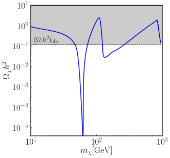
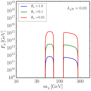
Figure 2: (Left) The behavior of $\Omega_{\chi}h^{2}$ as a function of $m_{\chi}$. The dip at $m_{\chi}\simeq 62.5$ GeV is due to the s-channel resonance from $h$. The broader valley starting from $m_{\chi}\simeq 125$ GeV is due to opening up of the $\chi_{1}\chi_{1}\to hh$ channel. The shaded region above the $\Omega_{c}h^{2}=0.12$ line is ruled out by the Planck experiment [1]. We allow the underabundance regions as the axion may account for the rest of the relic abundance. Other parameters chosen for this plot are as follows: $F_{a}=10^{10}\,{\rm GeV},\,M_{Q}=1\,{\rm TeV},\,f_{d}=0.1,\,\lambda_{\chi H}=0.03$, and $\lambda_{\zeta H}=\lambda_{\zeta\chi}=0.1$. (Right) The PQ scale $F_{a}$ needed for $\Omega_{a}h^{2}$ to satisfy the relic constraint $\Omega_{\chi}h^{2}+\Omega_{a}h^{2}=0.12$ for three different values of the misalignment angle $\theta_{a}$.

The large mass split between the two states prohibits the possibility of coannihilation of $\chi_{1}$ and $\chi_{2}$ during DM abundance formation. As noted before, the mass split $\Delta_{\chi}\sim\sqrt{F_{a}\epsilon_{\chi}}$ which, in the region of the parameter space of our interest, is much larger than $m_{\chi}$. For example, $\epsilon_{\chi}=1\,{\rm MeV}$ and $F_{a}=10^{10}\,{\rm GeV}$ imply $\Delta_{\chi}=1\,{\rm TeV}$. During freeze-out of $\chi_{1}$, its typical kinetic energy is of order $T_{\chi}\sim m_{\chi}/20$. Therefore, by this time the number density of $\chi_{2}$ particles is Boltzmann suppressed relative to $\chi_{1}$, $n_{2}/n_{1}\sim\exp{\left(-\Delta_{\chi}/T_{\chi}\right)}$ and hence is negligible. The DM relic abundance forms only through annihilations of $\chi_{1}$ into SM particles.

We show the dependence of the $\chi_{1}$ relic density as a function of its mass $m_{\chi}$ in the left panel of Fig. 2. We used micrOMEGAs5.0 [71] to numerically compute $\Omega_{\chi}h^{2}$. The behavior for very small and large $m_{\chi}$ can be understood as follows. For very small values of $m_{\chi}(\sim 10{\rm\ GeV})$, $\chi_{1}$ can annihilate only into the lighter quarks and the cross section is suppressed by the small Yukawa couplings resulting in overabundance of $\chi_{1}$. For $m_{\chi}\gg m_{t}$, the annihilation cross section is $1/m_{\chi}^{2}$ suppressed. Since the relic abundance is inversely proportional to the annihilation cross section, we expect the region around $m_{\chi}\approx 100$ GeV to give the correct ballpark value of the desired relic abundance.

The sharp dip at $m_{\chi}\simeq m_{h}/2\simeq 62.5$ GeV is due to the s-channel resonance from the $h$ propagator. As $m_{\chi}$ increases further from 62.5 GeV, the cross section falls leading to a sharp increase in the relic. When the $\chi_{1}$ is heavier than $h$, the new annihilation channel $\chi_{1}\chi_{1}\to hh$ opens up and dominates over all other channels. As a result, the relic abundance decreases, leading to the second dip. As $\chi_{1}$ becomes more massive, the relic increases again because of the decrease in annihilation cross section with the characteristic $1/m_{\chi}^{2}$ suppression. Note that we do not consider $m_{\chi}>M_{Q}$, as the colored $Q_{L,R}$ become the lightest dark sector particle.

In our analysis, we take the Planck (TT, TE, EE, lowP) measurement of the CDM energy density $\Omega_{c}h^{2}=0.12\pm 0.0012$ represented by the horizontal line labeled as $(\Omega h^{2})_{\rm obs}$ in the left panel of Fig. 2 [1]. The overabundance region, shown as a gray shade, is disallowed. However, the underabundance region is allowed since the axion abundance $\Omega_{a}h^{2}$ can account for the rest of the relic. Therefore, the observed relic abundance

$$\Omega_{c}h^{2}=\Omega_{\chi}h^{2}+\Omega_{a}h^{2}\,.$$ (13)

We note that $\Omega_{\chi}$ is virtually independent of $F_{a}$ due to the $v_{H}/F_{a}$ suppression in the couplings and mixing angle. Hence, $F_{a}$ is fixed by Eq. (13) via the $\Omega_{a}h^{2}$ term.

In the right panel of Fig. 2, we show the variation of $F_{a}$ with $m_{\chi}$ for three different values of $\theta_{a}$, for which the axion satisfies the relic constraint in the region, where the $\chi$ relic is underabundant. The result for different $\theta_{a}$ is just a rescaling of the value of $F_{a}$ according to Eq. (12). The gap in between the allowed lines account for the overabundance of DM due to the $\chi$.

We want to emphasize here that the interaction between $\zeta$ and $\chi$ fields does not affect the relic abundance of the axion and WIMP sectors. The $\epsilon_{\chi}\zeta^{*}\chi^{2}+{\rm h.c.}$ terms in Eq.(1) introduce interactions between $\chi_{1,2}$ and $a$, such as $\epsilon_{\chi}a\chi_{1}\chi_{2}$, $(\epsilon_{\chi}/F_{a})a^{2}\left(\chi_{1}^{2}-\chi_{2}^{2}\right)$ etc. The interaction involving $\chi_{2}$ is not important as its population is already Boltzmann suppressed. The interaction with $\chi_{1}$ is $(\epsilon_{\chi}/F_{a})$ suppressed and, therefore, not relevant for relic calculation of either species.

III.2 Direct detection of dark matter particles

The DM direct detection experiments look for scattering between the DM particles and nuclei in the detector material. Any interaction between the DM and the SM quarks or gluons in a given model leads to a possible signal in the direct detection experiments. Nonobservation of such a scattering signal in such experiments constrains the parameters of the model. In the present case, the dominant channel of interaction arises again through the $h\chi_{1}\chi_{1}$ coupling, since $h$ mediates the DM and SM quark scatterings.

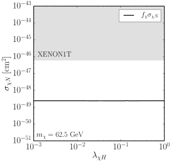
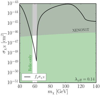
Figure 3: (Left) The rescaled $\chi_{1}$-nucleon scattering cross section $f_{\chi}\sigma_{\chi N}$ as a function of the coupling strength $\lambda_{\chi H}$. The gray shaded region shows the XENON1T upper bound for DM mass $m_{\chi}=62.5$ GeV. (Right) The rescaled $\chi_{1}$-nucleon scattering cross section as a function of $m_{\chi}$ for $\lambda_{\chi H}=0.14$. The XENON1T experiment excludes the gray shaded region. The green regions are excluded by the relic constraint itself, i.e., $f_{\chi}>1$.

The DM-nucleon scattering cross section $\sigma_{\chi N}$ is constant for very small $\lambda_{\chi H}$ because the coupling becomes independent of $\lambda_{\chi H}$. For very large $\lambda_{\chi H}$, the cross section increases as $\sim\lambda_{\chi H}^{2}$, as expected. In between, a dip occurs because of the cancellation of two terms appearing in the vertex factor of $h\chi_{1}\chi_{1}$ coupling [see Eq. (10)]. Note that this cancellation is entirely due to kinematics. There is neither any dynamical symmetry imposed to keep $m_{\chi}$ around $m_{h}/2$ nor any fine-tuning required. Since the enhancement of the cross sections is due to kinematics, the enhancement will remain stable under radiative corrections. Note that in this model, $\chi_{1}$ forms only a fraction $f_{\chi}$ of the total dark matter abundance [72, 43, 73, 74, 75, 76, 77]:

$$f_{\chi}=\frac{\Omega_{\chi}}{\Omega_{c}}\,.$$ (14)

Therefore the DM-nucleon cross section needs to be rescaled by $f_{\chi}$ before comparing it with the experimental results.

Note that in the literature, another convention of rescaling the DM-nucleon scattering cross section given by $f_{\chi}=\mathrm{Min}[1,\Omega_{\chi}/\Omega_{c}]$ exists, which saturates $f_{\chi}$ to unity in the overabundant region [78, 79]. However, in the context of our model, we use the prescription given in Eq. (14). This is well justified, since there exists a concrete prediction for calculating the DM relic in this model. Particularly, when there is a global overdensity, we do not assume that any other unknown mechanism can account for the relic density locally. While the direct and indirect detection constraints would depend on the choice of $f_{\chi}$, considering them with the relic bounds does not yield any additional allowed regions. Hence, our definition does not affect the final results.

Presently, the most stringent bound on the DM-nucleon cross section is given by the XENON1T$\times$1 yr data [51]. It is most sensitive to the DM mass in the range $10\,{\rm GeV}-1\,{\rm TeV}$ and the strongest upper bound quoted is $\sigma_{\chi N}\simeq 10^{-46}{\rm\ cm^{2}}$. The rescaled cross section $f_{\chi}\sigma_{\chi N}$ as a function of $\lambda_{\chi H}$ is shown in the left panel of Fig. 3. The cross section has a dip at $\lambda_{\chi H}=0.14$ and increases as $\sim\lambda_{\chi H}^{2}$ for larger values as explained before. However, $f_{\chi}$ on the other hand has a peak at the same parameter point because of inefficient relic annihilation due to vanishing of the $h\chi_{1}\chi_{1}$ coupling. Additionally, it has an inverse relation with $\lambda_{\chi H}$ for larger values: $f_{\chi}\sim\sigma_{\mathrm{ann}}^{-1}\sim\lambda_{\chi H}^{-2}$. Therefore, together the rescaled cross section $f\chi\sigma_{\chi N}$ does not have any features as shown in the left panel in Fig. 3.

We will show later that due to the stringent constraint, the only experimentally allowed region of DM mass turns out to be around $m_{\chi}\simeq 62.5$ GeV. This is shown in the right panel of Fig. 3, where we plot $f_{\chi}\sigma_{\chi N}$ as a function of $m_{\chi}$ for $\lambda_{\chi H}=0.14$. The gray region shows the XENON1T constraint. In passing, we comment that the region around $m_{\chi}\sim m_{h}$ is allowed by the relic constraint only if $\lambda_{\chi H}\lesssim 0.079$ or $\lambda_{\chi H}\gtrsim 0.25$. However, these regions are excluded by the XENON1T bound.

All the above bounds apply for $\chi_{1}$ as the DM candidate. However, direct detection experiments for axion need to follow a different search strategy because of its ultralow mass. There have been a few experimental efforts to look for axionic dark matter. For example, the ADMX experiment [80] uses a rf cavity to look for its interaction with the electromagnetic field. In the KSVZ model, the interaction strength between an axion and two photons is given by [19, 20]

$$g_{a\gamma}=-1.92\frac{\alpha}{2\pi F_{a}}\,,$$ (15)

where $\alpha$ is the fine structure constant. Presently, ADMX rules out a narrow region of the parameter space above $g_{a\gamma}\simeq 10^{-15}{\rm\ GeV^{-1}}$ ($F_{a}\simeq 10^{12}$ GeV) around $m_{a}\simeq 2\ \mu$eV. For a higher mass axion, the bound is even weaker. Another proposed experiment is CASPEr-Electric which will probe $F_{a}\gtrsim 10^{12}$ GeV for lighter axions [81]. Moreover, we should remember that these bounds assume that 100% CDM abundance is given by axion which is not be true in our model. These bounds are weaker than the upper limit on $F_{a}$ from the dark matter relic abundance, even after adjusting for the correct factor to cancel out the assumption and, hence, do not require special attention.

III.3 Dark matter annihilation signal

Various astrophysical observations hint that the present day Universe consists of galaxies sitting inside halolike structures formed by gravitational clustering of DM particles [82]. At the center of these halos, the DM density is high enough to scatter with each other and annihilate into SM particles. These final state particles would further decay and give rise to gamma-ray signals from various astrophysical objects, such as dwarf galaxies, the Milky Way center etc. We focus on bounds arising from gamma-ray signals due to such annihilations of DM particles.

We pay more attention to the DM mass around $m_{\chi}\simeq m_{h}/2=62.5$ GeV which is still allowed by the direct detection experiment data. The total annihilation is dominated by the $b\bar{b}$ channel ($\sim 90\%$). The rescaled annihilation rate $f_{\chi}^{2}(\sigma v)$ is shown in Fig. 4 as a solid black line. Note that here also the annihilation cross section is enhanced due to the s-channel resonance from the SM Higgs propagator. However, after rescaling with $f_{\chi}^{2}$, which is decreased at around $m_{\chi}\approx 62.5$ GeV, the annihilation rate $\sigma v$ shows a dip followed by a sharp increase around that point. The dependence on $\lambda_{\chi H}$ comes through the $g_{h\chi_{1}\chi_{1}}$ coupling.

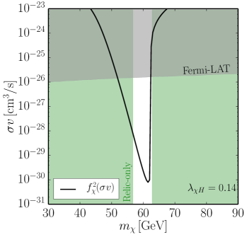
Figure 4: The rescaled annihilation rate $f_{\chi}^{2}(\sigma v)$ of $\chi_{1}\chi_{1}$ into $b\bar{b}$ in this model as a function of the mass of $\chi_{1}$ for $\lambda_{\chi H}=0.14$. The sharp dip is due to the s-channel resonance from the SM Higgs. The most stringent upper bound on this cross section is provided by the dwarf galaxy observation of the Fermi-LAT satellite data [83]. The gray shaded region is ruled out by the Fermi-LAT constraint. The green regions are excluded by the relic constraint itself, i.e., $f_{\chi}>1$.

There have been many experiments which have looked for DM annihilation signals from various astrophysical objects [83, 84, 85, 86]. At present, the most stringent upper bounds on the thermally averaged DM annihilation cross section $\langle\sigma v\rangle$ is given by the DES-Fermi-LAT joint gamma-ray search from the satellite galaxies of the Milky Way [83]. It is derived from 6 yr observation of 45 such objects by the LAT. They have relatively less amount of visible baryonic matter and the DM population is expected to dominate their matter density. In Fig. 4, we show this upper bound on the annihilation cross section due to Fermi-LAT as the gray shaded region. Note that the indirect detection bounds rule out most part of our parameter space, except a region around $m_{\chi}\simeq m_{h}/2$. In passing, we also note that the DM mass needed for the resonantly enhanced annihilation signal in the $b\bar{b}$ channel matches the result of the Galactic center excess analysis done in Ref. [87] within $1\sigma$ C.L. (also see [88]).

III.4 New physics searches at the LHC

In this subsection, we will focus on various signatures of the model at the LHC. The model has an extended scalar sector: apart from the SM Higgs boson $h_{0}$, there exists a scalar DM candidate $\chi_{1}$ and its heavier counterpart $\chi_{2}$, and another scalar field $\sigma_{0}$, which is the radial component of $\zeta$. As discussed earlier, $h_{0}$ and $\sigma_{0}$ mix with each other giving rise to physical states $h$ and $\sigma$. The mixing between $\sigma_{0}$ and $h_{0}$ changes the properties of $h$ from that of the SM Higgs via its coupling to SM particles as well as to the new states present in this model. Since various properties of the observed scalar particle at the LHC resemble that of the SM Higgs boson, we expect some constraints on the parameter space of the model from the measurement of the properties of the observed 125 GeV scalar.

One of the measurements that provides relevant information about the properties of the observed 125 GeV scalar is its signal strength. If the scalar decays to $X\in\{\ell^{\pm},q,g,Z,W$} and its conjugate $\bar{X}$, its signal strength is defined as

$$\mu_{X\bar{X}}=\frac{\sigma_{\text{exp}}(pp\rightarrow h)\times\text{BR}_{\text{exp}}(h\rightarrow X\bar{X})}{\sigma_{\text{SM}}(pp\rightarrow h)\times\text{BR}_{\text{SM}}(h\rightarrow X\bar{X})}\,,$$ (16)

where $\sigma_{\text{exp}}$ stands for the experimentally observed cross section of the process $pp\rightarrow h$ and $\text{BR}_{\text{exp}}$ is the experimentally observed branching ratio of the process $h\rightarrow X\bar{X}$. Similarly, $\sigma_{\text{SM}}$ and $\text{BR}_{\text{SM}}$ in Eq. (16) stand for the corresponding values predicted in the SM. We compare observed $\mu_{X\bar{X}}$ with the theoretically calculated $\mu_{X\bar{X}}$ from the model in different decay channels.

Due to the mixing, the physical scalar $h$ will have a $\cos\theta$ component in all the couplings with the SM. An additional decay mode of $h$ to $\chi_{1}\chi_{1}$ is possible if $m_{\chi}<m_{h}/2$. If the partial decay width of the new decay modes of $h$ is $\Gamma^{\text{new}}$, the signal strength of $h$ decaying to any SM particle pairs $X\bar{X}$ can be written as

$$\mu_{X\bar{X}}=\dfrac{\cos^{2}\theta}{1+\dfrac{\Gamma^{\text{new}}}{\cos^{2}\theta\ \Gamma^{\text{tot}}_{\text{SM}}}}\,,$$ (17)

where $\Gamma^{\text{tot}}_{\text{SM}}$ is the total decay width of SM Higgs boson.

Table 2: Measured values of the signal strengths of the 125 GeV observed scalar. The superscripts represent the production modes and the subscripts indicate the decay modes of the observed scalar $h$. The measurements are done by ATLAS and CMS at the LHC with $\sim 36$ fb^-1 luminosity at $\sqrt{s}=13$ TeV.

	ATLAS	CMS
$\mu^{\text{(ggF)}}_{WW^{*}}$	$1.21^{+0.22}_{-0.21}$ [89]	$1.38^{+0.21}_{-0.24}$ [90]
$\mu^{\text{(ggF)}}_{ZZ^{*}}$	$1.11^{+0.23}_{-0.21}$ [91]	$1.20^{+0.22}_{-0.21}$ [92]
$\mu_{\gamma\gamma}^{\text{(ggF+VH+VBF+ttH)}}$	$0.99^{+0.15}_{-0.14}$ [93]	$1.18^{+0.17}_{-0.14}$ [94]
$\mu_{b\bar{b}}^{\text{(VH)}}$	$1.20^{+0.42}_{-0.36}$ [95]	$1.06^{+0.31}_{-0.29}$ [96]
$\mu_{\tau\tau}^{\text{(ggF+VH+VBF)}}$	$1.43^{+0.43}_{-037}$ [97]	$1.09^{+0.27}_{-0.26}$ [98]

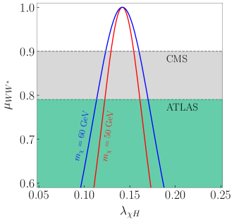
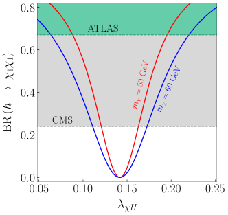
Figure 5: Bounds arising from (left) the Higgs signal strength in the $WW^{*}$ channel and (right) the invisible decay of the Higgs. The gray (green) shaded regions in both the plots are excluded by CMS (ATLAS) measurement at 95% C.L. The allowed regions are shown in white.

In Table 2, we tabulate the recent measurements of signal strength of the observed scalar $h$ by both ATLAS and CMS Collaborations at 13 TeV with $\sim 36$ pb^-1 integrated luminosity in different decay channels of $h$. The superscripts in the $\mu_{X\bar{X}}$ represent the production mode of the scalar $h$. For our analysis, we constrain the parameter space by imposing the value to be at 95% C.L. of the measured values, i.e., with $\pm 2\sigma$ around the measured central value. Since, in the model, $\mu_{X\bar{X}}$ is always below unity, it is the lower bound at 95% C.L. which will actually put constraints on the parameters.

In the left panel of Fig. 5, we show the variation of the signal strength of $h$ in the $WW^{*}$ channel as a function of $\lambda_{\chi H}$ for two different masses of $\chi_{1}$. As expected from Eq. (17), the variation is a Lorentzian, with a narrow width governed by $\Gamma^{\text{tot}}_{\text{SM}}$ and $m_{\chi}$. Since the coupling for $h$ to $\chi_{1}\chi_{1}$, as given in Eq. (10), vanishes at $\lambda_{\chi H}=2\lambda_{\zeta\chi}\left(\lambda_{H}-\lambda_{H}^{SM}\right)/\lambda_{\zeta H}$ ($\approx 0.14$ for the chosen benchmark point), the decay mode for the $h$ vanishes at that point, and hence the $\mu_{X\bar{X}}$ becomes 1 around that point. The gray (green) shaded region shows the area disallowed at 95% C.L. by the measurements by CMS (ATLAS) as indicated in the plot, and the allowed region is shown in white. Although the measurements for different decay channels of $h$ are listed in Table 2 for completeness, we only plotted $\mu^{\text{(ggF)}}_{WW^{*}}$, which gives the strongest bounds from the signal strength measurement.

We also study the bounds from the invisible decay of $h$ which arises from the decay channel $h\rightarrow\chi_{1}\chi_{1}$ for $m_{\chi}<m_{h}/2$ in this model. The BR of the decay can be written as

$$\text{BR}(h\to\chi_{1}\chi_{1})=\frac{1}{1+\cos^{2}\theta\,\dfrac{\Gamma^{\text{tot}}_{\text{SM}}}{\Gamma^{\text{new}}}}\,.$$ (18)

The dependence of BR$(h\to\chi_{1}\chi_{1})$ with the parameter $\lambda_{\chi H}$ is plotted in the right panel of Fig. 5 for two different masses of $\chi_{1}$. As in the case with the signal strength, the BR$(h\to\chi_{1}\chi_{1})$ vanishes at the point where the coupling of $h$ to $\chi_{1}\chi_{1}$, given by $g_{h\chi_{1}\chi_{1}}$ [see Eq. (10)], goes to zero. This feature is evident from the plot in the right panel of Fig. 5. Away from this point, the BR increases in both sides, tending to unity for a high value of $g_{h\chi_{1}\chi_{1}}$, which indicates that $\Gamma^{\text{new}}$ is the dominant decay mode, and all other modes are suppressed.

Table 3: Observed upper limit on the branching ratio of invisible decay of the scalar $h$.

	ATLAS	CMS
BR$\left(h\rightarrow\text{inv}\right)$	0.67 [99]	0.24 [100]

Nonobservation of this decay mode of the observed $125$ GeV scalar at the LHC, therefore, places an upper limit on the invisible decays of $h$. These upper limits are tabulated in Table 3. In the right panel of Fig. 5, the gray (green) shaded region is the area disallowed at 95% C.L. by CMS [100] (ATLAS [99]) measurements on the invisible decays of $125$ GeV scalar. It is therefore clear that only a small range of $\lambda_{\chi H}$, for which the BR curves fall within the white region, is allowed by current measurements.

At this point, it is worth mentioning that the trilinear coupling of $h$ is also modified due to the mixing with $\sigma_{0}$, which will change the di-Higgs production rate. Measurements for the trilinear coupling of $h$ as well as di-Higgs production have been carried out by both ATLAS [101] and CMS [102] in the di-Higgs channel. However, the upper bounds are well above the SM prediction due to lack of signal in the di-Higgs channel. Hence, much of the parameter space, especially the region of interest, of the model is not constrained by the measurement of trilinear coupling of $h$.

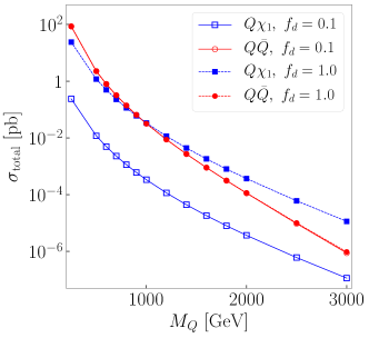
Figure 6: Variation of total production cross section for $Q\bar{Q}$ (in red) and for $Q\chi_{1}$ and $\bar{Q̄}\chi_{1}$ (in blue) in dijet+MET and in monojet+MET channels, respectively, at the LHC at $\sqrt{s}=13$ TeV as a function of $M_{Q}$ for $m_{\chi}=60$ GeV.

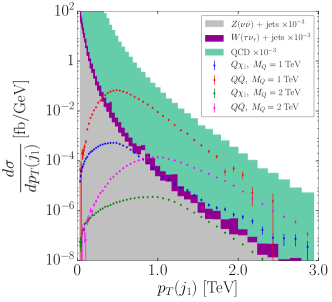
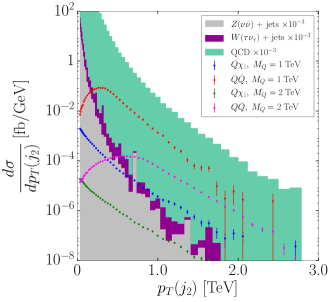
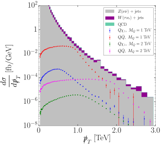
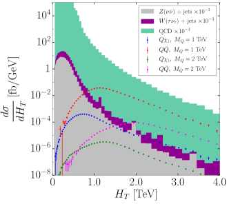
Figure 7: Differential distributions of signal and background events for dijet+MET and monojet+MET final states. Distributions are for (top left) $p_{T}$ of the leading jet, (top right) $p_{T}$ of the second jet, (bottom left) missing transverse energy $\not{p}_{T}$, and (bottom right) the scalar sum of $p_{T}$ of all the jets $H_{T}=\!\!\underset{j\,\in\,\text{jets}}{\sum}|\vec{p}_{T_{j}}|$ for different values of $M_{Q}$.

The model also predicts new particles at around GeV–TeV range, which can potentially be observed in a TeV collider. One such particle is the DM candidate $\chi_{1}$, which is weakly interacting and does not decay within the detector. If it is produced in the collider, it will not be detected and will contribute to the missing momentum in an event. The other particles, within the observable range of TeV collider, are the vectorlike quarks $Q_{L}$ and $Q_{R}$. Since these quarks are colored, they can be produced in a hadron collider and subsequently decay to a down-type quark and a $\chi_{1}$. The presence of $\chi_{1}$ will again contribute to the missing energy in the detector. The lack of agreement of such signals with those predicted at the TeV colliders will also put bounds on the parameter space of the model in consideration.

The contribution to the oblique parameters $(S,\ T$ and $U$) matters if the vectorlike quarks mix with our SM quarks. In that scenario, it contributes to the parameters strongly, depending on the mixing angle [103]. In our case, we do not directly have a SM top and $Q_{L,R}$ mixing because of the PQ symmetry. The mixing happens only through the $\zeta$-Higgs mixing, which induces a $h\bar{Q}_{L}Q_{R}$ term. This mixing is suppressed by $v_{H}/F_{a}$, which is super tiny. As a result, the contributions to the $S,\ T$ and $U$ parameters are not important.

Now, we turn to the discussion of direct production of the new particles at the LHC. The new particles, being charged under a PQ symmetry, should be produced in pairs. There are three different pairs of new particles that can be directly produced: $Q\bar{Q}$, $Q\chi_{1}$, and $\bar{Q}\chi_{1}$. Hence, these processes will contribute to the following final states: dijet $(2j)+$MET in case of $Q\bar{Q}$ production and monojet $(j)+$MET final state in case of $Q\chi_{1}$ and $\bar{Q}\chi_{1}$ production, where MET stands for missing transverse energy. In the rest of this section, we will discuss the constraints on the parameter space in view of the observation of the above-mentioned final states at the collider.

Since the $Q$s are colored, the cross section for the production of $Q\bar{Q}$ will be similar to that of the SM quarks and will be suppressed for higher masses. Figure 6 shows the variation of parton-level total production cross section for $Q\bar{Q}$ (in red) and for $Q\chi_{1}$ and $\bar{Q}\chi_{1}$ (in blue) in $2j+$MET and in $j+$MET channels, respectively, at the LHC at 13 TeV. The cross sections presented in Fig. 6 have been calculated at leading order using MadGraph5 [104] with the NNPDF2.3LO parton distribution function [105]. The production cross section of $Q\bar{Q}$ in the $2j+$MET channel has negligible dependence on $f_{d,s,b}$ since the dominant parton-level process for the production is $gg\to Q\bar{Q}$, which is independent of $f_{d,s,b}$. Hence, the two red curves, solid for $f_{d,s,b}=0.1$ and dashed for $f_{d,s,b}=1$, coincide with each other. However, the cross section for $Q\chi_{1}$ and $\bar{Q}\chi_{1}$ in $j+$MET channels scales as $f_{d,s,b}^{2}$ since the parton-level process involved in the production is $gq,\,g\bar{q}\to Q\chi_{1},\,\bar{Q}\,\chi_{1}$, whose amplitude is proportional to $f_{d,s,b}$. Note that the only possible decay mode of $Q$ is to a down-type quark and a $\chi_{1}$.

To estimate the signature of our model in collider experiments, events have been generated at partonic level using MadGraph5 with the NNPDF2.3LO parton distribution function using the Universal FeynRules Object (UFO) [106] files generated by FeynRules [68, 67] at a center-of-mass energy of 13 TeV; partons in the final state have been showered and hadronized using the parton shower in PYTHIA 8.210 [107] with 4C tune [108]. Stable particles have been clustered into anti-kT [109] jets of size 0.4 (used by both ATLAS and CMS) using the FastJet [110] software package; only the jets with $P_{T}$ more than 30 GeV have been considered for further analysis.

In Fig. 7, we present some important and representative differential distribution of some observables as are considered by experimental collaborations to search for signals. The top-left panel in the figure shows the distribution of $p_{T}$ of the leading jet while the panel in top right shows the distribution for $p_{T}$ of the second jet. In the bottom-left panel, we show the distribution of missing transverse energy ($\not{p}_{T}$). The bottom-right panel shows the distribution of $H_{T}=\!\!\!\underset{j\,\in\,\text{jets}}{\sum}|\vec{p}_{T_{j}}|$, which is the scalar sum of $p_{T}$ of all the jets. The major sources of the SM backgrounds for jets+MET are from the production of $Z$ decaying to $\nu\bar{\nu}$ and $W$ decaying to $\tau\nu_{\tau}$ in events with jets. Also QCD events are potential sources to contribute to the same final state. The distribution for these three backgrounds are plotted in four panels of Fig. 7. SM background samples have been generated with at leading order (LO) using MadGraph5 [104] with the NNPDF2.3LO parton distribution function [105] at center-of-mass energy of 13 TeV and PYTHIA 8.210 [107], with the same 4C tune [108] as used for generation of the signal sample, has been used for the simulation of fragmentation, parton shower, hadronization and underlying event. The distribution for QCD, $W$+jets, and $Z$+jets backgrounds are plotted with gray, purple, and green, respectively, with the same color convention in all four panels. From the figure, it is quite clear that the bumps for signals will not be significant enough to be observed above the expected fluctuation of the background.

Following the distribution in the experimental references [111, 112, 113, 55, 114, 115, 116, 117, 118], we carried out our analysis with the same distribution. As discussed earlier, the direct production of new particles will contribute to $2j+$MET and $j+$MET signals. There are few dedicated searches in these channels to search for dark matter signals [111, 112, 113, 55]. Few other models, especially supersymmetry (SUSY) in the R-parity conserving scenario, also lead to these kinds of signals. These searches have also been done by both CMS [114, 115] and ATLAS [116, 117, 118]. Though the results are given in terms of SUSY parameters or effective theory parameters, one can recast the result for a given model and check for its consistency. But these searches do not yield any further constraint in the parameter space in the model. A dedicated search for this model may give a stronger constraint, but the analysis of such a search is beyond the scope of this work.

IV Results

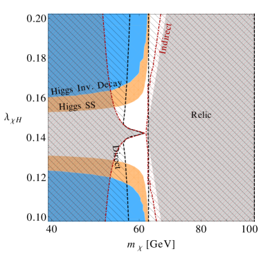
Figure 8: Allowed regions in the parameter space for the two-component axion-WIMP DM model. The gray shaded region shows the area ruled out by DM relic abundance constraint corresponding to the $2\sigma$ bound $\Omega_{c}h^{2}<0.12$ [1]. The black hatched lines show the regions of parameter space ruled out by the DM direct detection bounds from XENON1T$\times$1 yr experiment [51]. The hatched region within the red curve is ruled out by the DM annihilation data from DES-Fermi-LAT experiment [83]. The blue shaded region shows the bounds imposed due to the invisible decay modes of the Higgs, which is roughly $25\%$ of its branching ratio [89, 90]. The bound coming from the signal strength of the Higgs is shown in orange [99, 100]. The white, unshaded region represents the allowed parameter space in this model.

Our main results are summarized in Fig. 8. The relevant bounds coming from the different experiments are imposed on the region satisfying the DM relic density in the $\lambda_{\chi H}-m_{\chi}$ plane. The gray shaded region is ruled out by the relic constraints. We allow for both $\chi_{1}$ as well as the axion to contribute to the DM relic density. Hence the white region, corresponding to the $2\sigma$ bound $\Omega_{c}h^{2}<0.12$, represents the allowed parameter space, satisfying the relic density. As explained before, near $m_{\chi}\approx m_{h}/2$, the DM annihilation cross section is enhanced from the Higgs resonance, thereby decreasing the relic density of DM. This explains why the allowed region from relic is centered around $m_{\chi}=m_{h}/2$. Furthermore, there is a particular set of parameters for which $h\chi_{1}\chi_{1}$ coupling vanishes, leading to a rise in the relic density. This accounts for the peaklike structure in Fig. 8, which occurs at $\lambda_{\chi H}\sim 0.14$ for our choice of parameters.

The black hatched lines show the regions of parameter space ruled out by the direct detection bounds from XENON1T$\times$1 yr experiment. The hatched region within the red curve is ruled out by DES-Fermi-LAT joint gamma-ray search data from the Milky Way satellite galaxies. As is clearly seen, most of the allowed regions are ruled out, leaving behind a tiny window around in the $m_{\chi}-\lambda_{\chi H}$ plane. Clearly, this window is centered around $m_{\chi}\approx m_{h}/2$ and the value of $\lambda_{\chi H}$ for which the $h\chi_{1}\chi_{1}$ coupling vanishes.

The blue shaded region shows the bounds imposed due to the invisible decay modes of the Higgs, which is roughly $25\%$ of its branching ratio. More stringent bounds are imposed from the signal strength of the Higgs, which is shown in orange. These also help to rule out extra regions of the parameter space for larger as well as smaller values of $\lambda_{\chi H}$. We have also checked that the LHC bounds from production of $Q\bar{Q}$ are relatively weak; hence they do not impose any extra constraint on the model.

Thus, from the above figure, one concludes that only a small fraction of the model can still be accommodated from existing experimental bounds. This region, however, enjoys the advantage of an accidental cancellation of the couplings near $m_{h}/2$, thereby making it extremely difficult to rule out experimentally. This tiny window provides a breathing space for the model to survive.

V Summary and Discussions

In this paper, we have performed a comprehensive study of a two-component dark matter model, consisting of the QCD axion and an electromagnetic charge neutral scalar particle, both contributing to the relic density. The theory is symmetric under a global Peccei-Quinn symmetry, which can be spontaneously broken down to a residual $\mathbb{Z}_{2}$ symmetry. For concreteness, we have considered a specific model: the KSVZ model of the axion, augmented with an additional complex scalar. After spontaneous breaking of the PQ symmetry, the residual $\mathbb{Z}_{2}$ symmetry allows the lightest component of the complex scalar to be a DM candidate, apart from the axion. We have tested the model in the light of recent data from DM direct and indirect search experiments. Furthermore, we have also studied the different collider signatures of this model.

Although the observational and experimental constraints are found to be very restrictive, a synergy of the enhancement of DM annihilation from the Higgs resonance and the vanishing of the coupling between the Higgs and the dark matter leave room for future experimental investigation of this model. A large portion of the parameter space predicts overabundance of $\chi_{1}$ in the Universe and hence is not viable. In the remaining underabundant region of $\chi_{1}$, the axion can form the dominant part of the CDM. The viability of the axion being the CDM is being tested in several ongoing experiments. The latest dark matter direct and indirect detection experiments results further constrain this model. Moreover, these results are expected to improve the bounds by a few orders of magnitudes over the next few years which will subject this model to even tighter constraints. Although the bounds from the measurements of the properties of the Higgs at collider experiments are relatively weak, they still help to rule out an additional part of the parameter space. Future measurements of vectorlike quarks at high-luminosity and high-energy operating modes of the LHC can shed further light on the viability of this model.

Higher-order loop corrections may modify the DM direct detection cross section to some extent, as discussed in Refs. [119, 120, 121, 122]. Additionally, virtual internal bremsstrahlung in the annihilation of $\chi_{1}$ may introduce special features to the gamma-ray energy spectrum, making it easier to detect by some of the experiments [123]. However, these corrections were not taken into account here and will be addressed in a future work. Nevertheless, it is possible to add new particles to this simplistic model, e.g., an additional scalar, to enrich its phenomenology and evade some of the experimental bounds. This leaves room for future scopes of model building and investigation of observable signatures in high-energy experiments. In this work, we have calculated the prediction from our model with some natural choice for the couplings to compare with experimental data; but other values of the couplings can be explored to test the validity of the model on the basis of available experimental results. In conclusion, the two-component dark matter model, consisting of the WIMP and the axion, continues to survive, in spite of being tightly constrained.

*

Appendix A No Symmetry Breaking of $\chi$

The potential for $\chi$ before PQ-symmetry breaking is given by

$$V(\chi)=\lambda_{\chi}|\chi|^{4}+\mu_{\chi}^{2}|\chi|^{2}.$$ (19)

The minima for this potential occurs at $v_{\chi}=\sqrt{-\left(\mu_{\chi}^{2}/2\lambda_{\chi}\right)}$. We can always choose parameters such that $v_{\chi}<F_{a}$. This will prevent $\chi$ from developing a VEV before PQ-symmetry breaking. After PQ-symmetry breaking, the potential governing the evolution of the real components of $\chi$, viz. $\chi_{1}$ and $\chi_{2}$, is given by

$$V\left(\chi_{1},\chi_{2}\right)=\frac{\lambda_{\chi}}{4}\left(\chi_{1}^{2}+\chi_{2}^{2}\right)^{2}+\frac{1}{2}\,\mu_{\chi_{1}}^{2}\,\chi_{1}^{2}+\frac{1}{2}\,\mu_{\chi_{2}}^{2}\,\chi_{2}^{2},$$ (20)

where

$$\mu_{\chi_{1}}^{2}=\frac{1}{2}\left(2\mu_{\chi}^{2}+\lambda_{\zeta\chi}F_{a}^{2}-2\sqrt{2}\epsilon_{\chi}F_{a}\right),$$ (21)

$$\mu_{\chi_{2}}^{2}=\frac{1}{2}\left(2\mu_{\chi}^{2}+\lambda_{\zeta\chi}F_{a}^{2}+2\sqrt{2}\epsilon_{\chi}F_{a}\right).$$ (22)

There are four possibilities depending on the nature of the parameters:

1. $\mu_{\chi_{1}}^{2},\,\mu_{\chi_{2}}^{2}>0$.—This does not lead to a vev for $\chi_{1}$ or $\chi_{2}$.

2. $\mu_{\chi_{1}}^{2}>0$ and $\mu_{\chi_{2}}^{2}<0$.—This scenario is not possible since we choose $\epsilon_{\chi}>0$ in our analysis.

3. $\mu_{\chi_{1}}^{2}<0$ and $\mu_{\chi_{2}}^{2}>0$.—This parameter choice ensures no VEV for $\chi_{2}$. The minimization condition for $\chi_{1}$ then becomes

   $$\frac{\partial V(\chi_{1},\chi_{2})}{\partial\chi_{1}}\,\Bigg{|}_{\chi_{1}=\chi_{1_{\rm min}},\,\chi_{2}=0}=\lambda_{\chi}\chi_{1_{\rm min}}^{3}+\mu_{\chi_{1}}^{2}\chi_{1_{\rm min}}=0\,,$$

   which leads to $\chi_{1_{\rm min}}=0,{\rm\ and\ }\chi_{1_{\rm min}}=\pm\sqrt{-\left(\mu_{\chi_{1}}^{2}/\lambda_{\chi}\right)}$. Clearly, $\chi_{1_{\rm min}}=0$ is the solution for the maxima, and the other two solutions correspond to the minima.

4. $\mu_{\chi_{1}}^{2},\,\mu_{\chi_{2}}^{2}<0$.—This scenario is more involved and requires minimization with respect to both the fields:

   $$\frac{\partial V(\chi_{1},\chi_{2})}{\partial\chi_{1}}\,\Bigg{|}_{\chi_{1}=\chi_{1_{\rm min}},\,\chi_{2}=\chi_{2_{\rm min}}}$$ (24)

   $$\quad=\left[\lambda_{\chi}\left(\chi_{1_{\rm min}}^{2}+\chi_{2_{\rm min}}^{2}\right)+\mu_{\chi_{1}}^{2}\right]\chi_{1_{\rm min}}=0,$$

   $$\& \frac{\partial V(\chi_{1},\chi_{2})}{\partial\chi_{2}}\,\Bigg{|}_{\chi_{1}=\chi_{1_{\rm min}},\,\chi_{2}=\chi_{2_{\rm min}}}$$ (25)

   $$\quad=\left[\lambda_{\chi}\left(\chi_{1_{\rm min}}^{2}+\chi_{2_{\rm min}}^{2}\right)+\mu_{\chi_{2}}^{2}\right]\chi_{2_{\rm min}}=0.$$

   The above set of equations permits the following solutions:

   $$({\rm soln:a}) \quad\chi_{1_{\rm min}}=\chi_{2_{\rm min}}=0,$$ (26)

   $$({\rm soln:b}) \quad\chi_{1_{\rm min}}=0,\ \chi_{2_{\rm min}}=\pm\sqrt{-\frac{\mu_{\chi_{2}}^{2}}{\lambda_{\chi}}},$$ (27)

   $${\rm and\ }({\rm soln:c})\quad\chi_{1_{\rm min}}=\pm\sqrt{-\frac{\mu_{\chi_{1}}^{2}}{\lambda_{\chi}}},\ \chi_{2_{\rm min}}=0.~{}~{}$$ (28)

   To determine which solution corresponds to a minima, we take a further derivative to get

   $$\frac{\partial^{2}V(\chi_{1},\chi_{2})}{\partial\chi_{1}^{2}}=\lambda_{\chi}\left(3\chi_{1}^{2}+\chi_{2}^{2}\right)+\mu_{\chi_{1}}^{2},$$ (29)

   $$\frac{\partial^{2}V(\chi_{1},\chi_{2})}{\partial\chi_{2}^{2}}=\lambda_{\chi}\left(\chi_{1}^{2}+3\chi_{2}^{2}\right)+\mu_{\chi_{2}}^{2},$$ (30)

   $$\frac{\partial^{2}V(\chi_{1},\chi_{2})}{\partial\chi_{1}\partial\chi_{2}}=2\,\lambda_{\chi}\,\chi_{1}\,\chi_{2}.$$ (31)

   The nature of the solutions in Eqs. (26, 27, and 28) are determined by the determinant and trace of the Hessian. This gives the following conditions:

   • Det = $0$ and Tr = $0$.—Further analysis is required to tell the nature of this point. For this solution, $V(\chi_{1}=0,\chi_{2}=0)=0$, which is bigger than the values at other solutions. So, even if it is a minima, it is not a global minima.

   • Det = $4\sqrt{2}\epsilon_{\chi}F_{a}\mu_{\chi_{2}}^{2}<0$.—This corresponds to a saddle point solution.

   • Det = $-4\sqrt{2}\epsilon_{\chi}F_{a}\mu_{\chi_{1}}^{2}>0$ and Tr = $\mu_{\chi_{2}}^{2}-3\mu_{\chi_{1}}^{2}>0$.—This is a minima.

This analysis confirms that $\chi_{2}$ will never get a VEV. Whether $\chi_{1}$ will get a VEV or not depends on the choice of the parameters. For our model to be valid, we need to choose parameters in such a way so that $\chi_{1_{\rm min}}<v_{H}$. This will prevent $\chi_{1}$ from developing a VEV before electroweak symmetry breaking. After electroweak symmetry breaking, however, $\chi_{1}$ gets real mass as given in Eq. (7). We can quickly estimate the value of $\chi_{1_{\rm min}}$ for the parameters of our model. The values of $\chi_{1_{\rm min}}$ as a function of $\lambda_{\chi}$ are shown in Fig. 9 for different values of $m_{\chi}$. Clearly, for natural values of the coupling $\lambda_{\chi}\gtrsim 0.05$, global minima of the potential in Eq. (20) occurs for values $\chi_{1_{\rm min}}$ below $v_{H}$, which prevents $\chi_{1}$ from developing a VEV before electroweak symmetry breaking. After electroweak symmetry breaking, both $\chi_{1}$ and $\chi_{2}$ get real mass. So, we can always choose parameters in our model in such a way that neither $\chi$ nor $\chi_{1}$ or $\chi_{2}$ develops a VEV throughout the entire symmetry-breaking process of $\zeta$ and $H$.

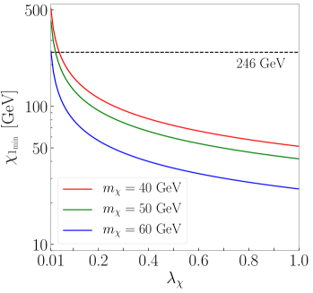
Figure 9: Values of $\chi_{1_{\rm min}}$ for our parameter choices as a function of $\lambda_{\chi}$ for different values of $m_{\chi}$.

References

- Ade et al. [2016] P. A. R. Ade et al. (Planck Collaboration), Astron. Astrophys. 594, A13 (2016), arXiv:1502.01589 [astro-ph.CO] .
- Jungman et al. [1996] G. Jungman, M. Kamionkowski, and K. Griest, Phys. Rep. 267, 195 (1996), arXiv:hep-ph/9506380 [hep-ph] .
- Pagels and Primack [1982] H. Pagels and J. R. Primack, Phys. Rev. Lett. 48, 223 (1982).
- Kolb and Slansky [1984] E. W. Kolb and R. Slansky, Phys. Lett. 135B, 378 (1984).
- Ellis et al. [1984] J. R. Ellis, J. S. Hagelin, D. V. Nanopoulos, K. A. Olive, and M. Srednicki, Nucl. Phys. B238, 453 (1984).
- Bertone et al. [2005] G. Bertone, D. Hooper, and J. Silk, Phys. Rep. 405, 279 (2005), arXiv:hep-ph/0404175 [hep-ph] .
- Bergström, Lars [2000] L. Bergström, Rep. Prog. Phys. 63, 793 (2000), arXiv:hep-ph/0002126 [hep-ph] .
- Bertone and Hooper [2016] G. Bertone and D. Hooper, Rev. Mod. Phys. 90, 045002 (2018), arXiv:1605.04909 [astro-ph.CO] .
- Gondolo and Gelmini [1991] P. Gondolo and G. Gelmini, Nucl. Phys. B360, 145 (1991).
- Griest and Seckel [1991] K. Griest and D. Seckel, Phys. Rev. D43, 3191 (1991).
- Steigman et al. [2012] G. Steigman, B. Dasgupta, and J. F. Beacom, Phys. Rev. D86, 023506 (2012), arXiv:1204.3622 [hep-ph] .
- Steigman and Turner [1985] G. Steigman and M. S. Turner, Nucl. Phys. B253, 375 (1985).
- Peccei [2008] R. D. Peccei, Lect. Notes Phys. 741, 3 (2008), arXiv:hep-ph/0607268 [hep-ph] .
- Crewther et al. [1979] R. J. Crewther, P. Di Vecchia, G. Veneziano, and E. Witten, Phys. Lett. 88B, 123 (1979); [Erratum: Phys. Lett. 91B, 487 (1980).
- Kim and Carosi [2010] J. E. Kim and G. Carosi, Rev. Mod. Phys. 82, 557 (2010), arXiv:0807.3125 [hep-ph] .
- Peccei and Quinn [1977] R. D. Peccei and H. R. Quinn, Phys. Rev. Lett. 38, 1440 (1977).
- Wilczek [1978] F. Wilczek, Phys. Rev. Lett. 40, 279 (1978).
- Weinberg [1978] S. Weinberg, Phys. Rev. Lett. 40, 223 (1978).
- Kim [1979] J. E. Kim, Phys. Rev. Lett. 43, 103 (1979).
- Shifman et al. [1980] M. A. Shifman, A. I. Vainshtein, and V. I. Zakharov, Nucl. Phys. B166, 493 (1980).
- Kim [1987] J. E. Kim, Phys. Rep. 150, 1 (1987).
- Dine et al. [1981] M. Dine, W. Fischler, and M. Srednicki, Phys. Lett. 104B, 199 (1981).
- Zhitnitsky [1980] A. R. Zhitnitsky, Yad. Fiz. 31, 497 (1980) [Sov. J. Nucl. Phys. 31, 260 (1980)].
- Chikashige et al. [1981] Y. Chikashige, R. N. Mohapatra, and R. D. Peccei, Phys. Lett. 98B, 265 (1981).
- Gelmini and Roncadelli [1981] G. B. Gelmini and M. Roncadelli, Phys. Lett. 99B, 411 (1981).
- Wilczek [1982] F. Wilczek, Phys. Rev. Lett. 49, 1549 (1982).
- Berezhiani and Khlopov [1990] Z. G. Berezhiani and M. Yu. Khlopov, Yad. Fiz. 51, 1157 (1990) [Sov. J. Nucl. Phys. 51, 739 (1990)].
- Jaeckel [2014] J. Jaeckel, Phys. Lett. B732, 1 (2014), arXiv:1311.0880 [hep-ph] .
- Witten [1984] E. Witten, Phys. Lett. 149B, 351 (1984).
- Conlon [2006] J. P. Conlon, JHEP 05, 078 (2006), arXiv:hep-th/0602233 [hep-th] .
- Cicoli et al. [2012] M. Cicoli, M. Goodsell, and A. Ringwald, JHEP 10, 146 (2012), arXiv:1206.0819 [hep-th] .
- Georgi et al. [1981] H. M. Georgi, L. J. Hall, and M. B. Wise, Nucl. Phys. B192, 409 (1981).
- Dias et al. [2014] A. G. Dias, A. C. B. Machado, C. C. Nishi, A. Ringwald, and P. Vaudrevange, JHEP 06, 037 (2014), arXiv:1403.5760 [hep-ph] .
- Choi et al. [2009] K.-S. Choi, H. P. Nilles, S. Ramos-Sanchez, and P. K. S. Vaudrevange, Phys. Lett. B675, 381 (2009), arXiv:0902.3070 [hep-th] .
- Kuster et al. [2008] M. Kuster, G. Raffelt, and B. Beltran, Lect. Notes Phys. 741, 1 (2008).
- Marsh [2016] D. J. E. Marsh, Phys. Rep. 643, 1 (2016), arXiv:1510.07633 [astro-ph.CO] .
- Kim [2007] J. E. Kim, in Proceedings of the 23rd International Symposium on Lepton and Photon Interactions at High Energies, LP2007, Daegu, South Korea, 2007 (Kyungpook National University Press, Daegu, 2007) pp. 408–420, arXiv:0711.1708 [hep-ph] .
- Preskill et al. [1983] J. Preskill, M. B. Wise, and F. Wilczek, Phys. Lett. B120, 127 (1983).
- Abbott and Sikivie [1983] L. F. Abbott and P. Sikivie, Phys. Lett. B120, 133 (1983).
- Dine and Fischler [1983] M. Dine and W. Fischler, Phys. Lett. B120, 137 (1983).
- Zurek [2009] K. M. Zurek, Phys. Rev. D79, 115002 (2009), arXiv:0811.4429 [hep-ph] .
- Biswas et al. [2013] A. Biswas, D. Majumdar, A. Sil, and P. Bhattacharjee, JCAP 1312, 049 (2013), arXiv:1301.3668 [hep-ph] .
- Bhattacharya et al. [2013] S. Bhattacharya, A. Drozd, B. Grzadkowski, and J. Wudka, JHEP 10, 158 (2013), arXiv:1309.2986 [hep-ph] .
- Dutta Banik et al. [2017] A. Dutta Banik, M. Pandey, D. Majumdar, and A. Biswas, Eur. Phys. J. C77, 657 (2017), arXiv:1612.08621 [hep-ph] .
- Arcadi et al. [2016] G. Arcadi, C. Gross, O. Lebedev, Y. Mambrini, S. Pokorski, and T. Toma, JHEP 12, 081 (2016), arXiv:1611.00365 [hep-ph] .
- Alves et al. [2016] A. Alves, D. A. Camargo, A. G. Dias, R. Longas, C. C. Nishi, and F. S. Queiroz, JHEP 10, 015 (2016), arXiv:1606.07086 [hep-ph] .
- Pandey et al. [2018] M. Pandey, D. Majumdar, and K. P. Modak, JCAP 1806, 023 (2018), arXiv:1709.05955 [hep-ph] .
- Chakraborti et al. [2018] S. Chakraborti, A. Dutta Banik, and R. Islam, Eur. Phys. J. C79, 662 (2019), arXiv:1810.05595 [hep-ph] .
- Dasgupta et al. [2014] B. Dasgupta, E. Ma, and K. Tsumura, Phys. Rev. D89, 041702 (2014), arXiv:1308.4138 [hep-ph] .
- Krauss and Wilczek [1989] L. M. Krauss and F. Wilczek, Phys. Rev. Lett. 62, 1221 (1989).
- Aprile et al. [2018] E. Aprile et al. (XENON Collaboration), Phys. Rev. Lett. 121, 111302 (2018), arXiv:1805.12562 [astro-ph.CO] .
- Athron et al. [2017] P. Athron et al. (GAMBIT Collaboration), Eur. Phys. J. C77, 568 (2017), arXiv:1705.07931 [hep-ph] .
- Aaboud et al. [2016] M. Aaboud et al. (ATLAS Collaboration), Phys. Rev. D94, 032005 (2016), arXiv:1604.07773 [hep-ex] .
- Sirunyan et al. [2017a] A. M. Sirunyan et al. (CMS Collaboration), JHEP 07, 014 (2017a), arXiv:1703.01651 [hep-ex] .
- Sirunyan et al. [2018a] A. M. Sirunyan et al. (CMS Collaboration), Phys. Rev. D97, 092005 (2018a), arXiv:1712.02345 [hep-ex] .
- Adler [1969] S. L. Adler, Phys. Rev. 177, 2426 (1969).
- Bell and Jackiw [1969] J. S. Bell and R. Jackiw, Nuovo Cim. A60, 47 (1969).
- Raffelt and Seckel [1988] G. Raffelt and D. Seckel, Phys. Rev. Lett. 60, 1793 (1988).
- Aad et al. [2012] G. Aad et al. (ATLAS collaboration), Phys. Lett. B716, 1 (2012), arXiv:1207.7214 [hep-ex] .
- Chatrchyan et al. [2012] S. Chatrchyan et al. (CMS collaboration), Phys. Lett. B716, 30 (2012), arXiv:1207.7235 [hep-ex] .
- Tanabashi et al. [2018] M. Tanabashi et al. (Particle Data Group), Phys. Rev. D98, 030001 (2018).
- Giddings and Strominger [1988] S. B. Giddings and A. Strominger, Nucl. Phys. B307, 854 (1988).
- Coleman [1988] S. R. Coleman, Nucl. Phys. B310, 643 (1988).
- Kamionkowski and March-Russell [1992] M. Kamionkowski and J. March-Russell, Phys. Lett. B282, 137 (1992), arXiv:hep-th/9202003 [hep-th] .
- Ghigna et al. [1992] S. Ghigna, M. Lusignoli, and M. Roncadelli, Phys. Lett. B283, 278 (1992).
- Gross et al. [1981] D. J. Gross, R. D. Pisarski, and L. G. Yaffe, Rev. Mod. Phys. 53, 43 (1981).
- Christensen and Duhr [2009] N. D. Christensen and C. Duhr, Comput. Phys. Commun. 180, 1614 (2009), arXiv:0806.4194 [hep-ph] .
- Alloul et al. [2014] A. Alloul, N. D. Christensen, C. Degrande, C. Duhr, and B. Fuks, Comput. Phys. Commun. 185, 2250 (2014), arXiv:1310.1921 [hep-ph] .
- Bae et al. [2008] K. J. Bae, J.-H. Huh, and J. E. Kim, JCAP 0809, 005 (2008), arXiv:0806.0497 [hep-ph] .
- Sikivie [1982] P. Sikivie, Phys. Rev. Lett. 48, 1156 (1982).
- Bélanger et al. [2018] G. Bélanger, F. Boudjema, A. Goudelis, A. Pukhov, and B. Zaldivar, Comput. Phys. Commun. 231, 173 (2018), arXiv:1801.03509 [hep-ph] .
- Cao et al. [2007] Q.-H. Cao, E. Ma, J. Wudka, and C. P. Yuan, (2007), arXiv:0711.3881 [hep-ph] .
- Ilnicka et al. [2016] A. Ilnicka, M. Krawczyk, and T. Robens, Phys. Rev. D93, 055026 (2016), arXiv:1508.01671 [hep-ph] .
- Bhattacharya et al. [2017] S. Bhattacharya, P. Poulose, and P. Ghosh, JCAP 1704, 043 (2017), arXiv:1607.08461 [hep-ph] .
- Ahmed et al. [2018] A. Ahmed, M. Duch, B. Grzadkowski, and M. Iglicki, Eur. Phys. J. C78, 905 (2018), arXiv:1710.01853 [hep-ph] .
- Betancur and Zapata [2018] A. Betancur and . Zapata, Phys. Rev. D98, 095003 (2018), arXiv:1809.04990 [hep-ph] .
- Borah et al. [2019] D. Borah, R. Roshan, and A. Sil, Phys. Rev. D100, 055027 (2019), arXiv:1904.04837 [hep-ph] .
- Gaisser et al. [1986] T. K. Gaisser, G. Steigman, and S. Tilav, Phys. Rev. D 34, 2206 (1986).
- Bottino et al. [1997] A. Bottino, F. Donato, G. Mignola, S. Scopel, P. Belli, and A. Incicchitti, Phys. Lett. B402, 113 (1997), arXiv:hep-ph/9612451 [hep-ph] .
- Asztalos et al. [2010] S. J. Asztalos, G. Carosi, C. Hagmann, D. Kinion, K. van Bibber, M. Hotz, L. J. Rosenberg, G. Rybka, J. Hoskins, J. Hwang, P. Sikivie, D. B. Tanner, R. Bradley, J. Clarke (ADMX Collaboration), Physical Review Letters 104, 041301 (2010), arXiv:0910.5914 [astro-ph.CO] .
- Budker et al. [2014] D. Budker, P. W. Graham, M. Ledbetter, S. Rajendran, and A. Sushkov, Phys. Rev. X4, 021030 (2014), arXiv:1306.6089 [hep-ph] .
- Clowe et al. [2006] D. Clowe, M. Bradac, A. H. Gonzalez, M. Markevitch, S. W. Randall, C. Jones, and D. Zaritsky, Astrophys. J. 648, L109 (2006), arXiv:astro-ph/0608407 [astro-ph] .
- Albert et al. [2017] A. Albert et al. (DES, Fermi-LAT Collaboration), Astrophys. J. 834, 110 (2017), arXiv:1611.03184 [astro-ph.HE] .
- Abdallah et al. [2016] H. Abdallah et al. (H.E.S.S. Collaboration), Phys. Rev. Lett. 117, 111301 (2016), arXiv:1607.08142 [astro-ph.HE] .
- Ahnen et al. [2018] M. L. Ahnen et al. (MAGIC Collaboration), JCAP 1803, 009 (2018), arXiv:1712.03095 [astro-ph.HE] .
- Aartsen et al. [2017] M. G. Aartsen et al. (IceCube Collaboration), Eur. Phys. J. C77, 627 (2017), arXiv:1705.08103 [hep-ex] .
- Huang et al. [2013] W. C. Huang, A. Urbano, and W. Xue, arXiv:1307.6862 [hep-ph] .
- Calore et al. [2015] F. Calore, I. Cholis, and C. Weniger, JCAP 1503, 038 (2015), arXiv:1409.0042 [astro-ph.CO] .
- Aaboud et al. [2019] M. Aaboud et al. (ATLAS Collaboration), Phys. Lett. B789, 508 (2019), arXiv:1808.09054 [hep-ex] .
- Sirunyan et al. [2019a] A. M. Sirunyan et al. (CMS Collaboration), Phys. Lett. B791, 96 (2019a), arXiv:1806.05246 [hep-ex] .
- Aaboud et al. [2018a] M. Aaboud et al. (ATLAS Collaboration), JHEP 03, 095 (2018a), arXiv:1712.02304 [hep-ex] .
- Sirunyan et al. [2017b] A. M. Sirunyan et al. (CMS Collaboration), JHEP 11, 047 (2017b), arXiv:1706.09936 [hep-ex] .
- Aaboud et al. [2018b] M. Aaboud et al. (ATLAS Collaboration), Phys. Rev. D98, 052005 (2018), arXiv:1802.04146 [hep-ex] .
- Sirunyan et al. [2019b] A. M. Sirunyan et al. (CMS Collaboration), Eur. Phys. J. C79, 421 (2019b), arXiv:1809.10733 [hep-ex] .
- Aaboud et al. [2017a] M. Aaboud et al. (ATLAS Collaboration), JHEP 12, 024 (2017a), arXiv:1708.03299 [hep-ex] .
- Sirunyan et al. [2018b] A. M. Sirunyan et al. (CMS Collaboration), Phys. Lett. B780, 501 (2018b), arXiv:1709.07497 [hep-ex] .
- Aad et al. [2015] G. Aad et al. (ATLAS Collaboration), JHEP 04, 117 (2015), arXiv:1501.04943 [hep-ex] .
- Sirunyan et al. [2018c] A. M. Sirunyan et al. (CMS Collaboration), Phys. Lett. B779, 283 (2018c), arXiv:1708.00373 [hep-ex] .
- Aaboud et al. [2018c] M. Aaboud et al. (ATLAS Collaboration), Phys. Lett. B776, 318 (2018c), arXiv:1708.09624 [hep-ex] .
- Collaboration [2018c] CMS Collaboration, Technical Report No. CMS-PAS-HIG-17-023, 2018, https://cds.cern.ch/record/2308434.
- Aad et al. [2020] G. Aad et al. (ATLAS Collaboration), Phys. Lett. B800, 135103 (2020), arXiv:1906.02025 [hep-ex] .
- Sirunyan et al. [2018d] A. M. Sirunyan et al. (CMS Collaboration), Phys. Lett. B788, 7 (2019), arXiv:1806.00408 [hep-ex] .
- Dawson and Furlan [2012] S. Dawson and E. Furlan, Phys. Rev. D86, 015021 (2012), arXiv:1205.4733 [hep-ph] .
- Alwall et al. [2014] J. Alwall, R. Frederix, S. Frixione, V. Hirschi, F. Maltoni, O. Mattelaer, H. S. Shao, T. Stelzer, P. Torrielli, and M. Zaro, JHEP 07, 079 (2014), arXiv:1405.0301 [hep-ph] .
- Ball et al. [2015] R. D. Ball et al. (NNPDF Collaboration), JHEP 04, 040 (2015), arXiv:1410.8849 [hep-ph] .
- Degrande et al. [2012] C. Degrande, C. Duhr, B. Fuks, D. Grellscheid, O. Mattelaer, and T. Reiter, Comput. Phys. Commun. 183, 1201 (2012), arXiv:1108.2040 [hep-ph] .
- Sjöstrand et al. [2015] T. Sjöstrand, S. Ask, J. R. Christiansen, R. Corke, N. Desai, P. Ilten, S. Mrenna, S. Prestel, C. O. Rasmussen, and P. Z. Skands, Comput. Phys. Commun. 191, 159 (2015), arXiv:1410.3012 [hep-ph] .
- Sjostrand et al. [2006] T. Sjöstrand, S. Mrenna, and P. Z. Skands, JHEP 05, 026 (2006), arXiv:hep-ph/0603175 [hep-ph] .
- Cacciari et al. [2008] M. Cacciari, G. P. Salam, and G. Soyez, JHEP 04, 063 (2008), arXiv:0802.1189 [hep-ph] .
- Cacciari et al. [2012] M. Cacciari, G. P. Salam, and G. Soyez, Eur. Phys. J. C72, 1896 (2012), arXiv:1111.6097 [hep-ph] .
- Aaboud et al. [2018d] M. Aaboud et al. (ATLAS Collaboration), Eur. Phys. J. C78, 18 (2018d), arXiv:1710.11412 [hep-ex] .
- Aaboud et al. [2018e] M. Aaboud et al. (ATLAS Collaboration), JHEP 01, 126 (2018e), arXiv:1711.03301 [hep-ex] .
- Khachatryan et al. [2015] V. Khachatryan et al. (CMS Collaboration), Eur. Phys. J. C75, 235 (2015), arXiv:1408.3583 [hep-ex] .
- Sirunyan et al. [2017c] A. M. Sirunyan et al. (CMS Collaboration), Phys. Rev. D96, 032003 (2017c), arXiv:1704.07781 [hep-ex] .
- Sirunyan et al. [2017d] A. M. Sirunyan et al. (CMS Collaboration), Eur. Phys. J. C77, 710 (2017d), arXiv:1705.04650 [hep-ex] .
- Aaboud et al. [2018f] M. Aaboud et al. (ATLAS Collaboration), JHEP 06, 107 (2018f), arXiv:1711.01901 [hep-ex] .
- Aaboud et al. [2017b] M. Aaboud et al. (ATLAS Collaboration), Phys. Rev. D97, 112001 (2018), arXiv:1712.02332 [hep-ex] .
- Aaboud et al. [2017c] M. Aaboud et al. (ATLAS Collaboration), JHEP 12, 085 (2017c), arXiv:1709.04183 [hep-ex] .
- Klasen et al. [2013] M. Klasen, C. E. Yaguna, and J. D. Ruiz-Alvarez, Phys. Rev. D87, 075025 (2013), arXiv:1302.1657 [hep-ph] .
- Ibarra and Wild [2015] A. Ibarra and S. Wild, JCAP 1505, 047 (2015), arXiv:1503.03382 [hep-ph] .
- Klasen et al. [2016] M. Klasen, K. Kovarik, and P. Steppeler, Phys. Rev. D94, 095002 (2016), arXiv:1607.06396 [hep-ph] .
- Abe et al. [2018] T. Abe, M. Fujiwara, and J. Hisano, JHEP 02, 028 (2019), arXiv:1810.01039 [hep-ph] .
- Chowdhury et al. [2018] D. Chowdhury, A. M. Iyer, and R. Laha, JHEP 05, 152 (2018), arXiv:1601.06140 [hep-ph] .