Spectrophotometric parallaxes with linear models:
Accurate distances for luminous red-giant stars

Abstract

With contemporary infrared spectroscopic surveys like APOGEE, red-giant stars can be observed to distances and extinctions at which Gaia parallaxes are not highly informative. Yet the combination of effective temperature, surface gravity, composition, and age—all accessible through spectroscopy—determines a giant’s luminosity. Therefore spectroscopy plus photometry should enable precise spectrophotometric distance estimates. Here we use the APOGEE–Gaia–2MASS–WISE overlap to train a data-driven model to predict parallaxes for red-giant branch stars with $0<\log g\leq 2.2$ (more luminous than the red clump). We employ (the exponentiation of) a linear function of APOGEE spectral pixel intensities and multi-band photometry to predict parallax spectrophotometrically. The model training involves no logarithms or inverses of the Gaia parallaxes, and needs no cut on the Gaia parallax signal-to-noise ratio. It includes an L1 regularization to zero out the contributions of uninformative pixels. The training is performed with leave-out subsamples such that no star’s astrometry is used even indirectly in its spectrophotometric parallax estimate. The model implicitly performs a reddening and extinction correction in its parallax prediction, without any explicit dust model. We assign to each star in the sample a new spectrophotometric parallax estimate; these parallaxes have uncertainties of a few to 15 percent, depending on data quality, which is more precise than the Gaia parallax for the vast majority of targets, and certainly any stars more than a few kpc distance. We obtain 10-percent distance estimates out to heliocentric distances of 20 kpc, and make global maps of the Milky Way’s disk.

 

Section 1 Introduction

If we want to make precise kinematic and element-abundance maps of the Milky Way disk out to large heliocentric radii, and especially through the extinction to the other side of the Galactic Center, we will need to make use of luminous red giants, and we will need to observe in the infrared. These arguments motivate the APOGEE (Majewski et al. 2017), APOGEE-2, and SDSS-V (Kollmeier et al. 2017) projects, which take spectra in the infrared, and deliver detailed abundances along the entire red-giant branch up to the tip. The maps made with these data will reveal the dynamics of the Milky Way and its disk, and show us how and where stars form, and how they migrate around the disk with time.

As we operate these spectroscopic surveys, the Gaia Mission (Gaia Collaboration et al. 2016) has also been revolutionizing our view of the disk. It delivers good proper motions over most of the Galaxy, and extremely valuable parallax information locally. However, Gaia does not deliver precise geometric parallaxes over a large fraction of the disk, and certainly not in the dusty and crowded regions. For these reasons, the value of Gaia in these infrared spectroscopy projects is not to deliver distance information directly, but rather to calibrate stellar models, which then deliver distance information through relationships between stellar luminosities and spectral characteristics.

Luminous red-giant stars are valuable for mapping the Milky Way disk for a number of reasons, only one of which is their great luminosities (and hence brightnesses even at large distance). They are very common stars, much more frequent than distance-indicating stars like Cepheids. They are produced by stellar populations at all metallicities and almost all ages, so they can be found in all parts of the Galaxy. They have temperatures and surface gravities such that it is straightforward to spectroscopically measure metallicities, detailed chemical abundances, and stellar parameters, even including ages (Martig et al. 2016; Ness et al. 2016). The red-giant branch is photometrically near-orthogonal to reddening vectors by dust, so they are easy to de-redden or dust-correct. And finally, in physical models of red giants, their predicted luminosities are simple functions of composition, surface gravity, temperature, and age. Thus, if we can measure these properties of red giants, we can (in principle) predict their luminosities and use them as standard candles. That is, red giants are standardizable candles.

In this project, we develop purely data-driven techniques to predict red-giant parallaxes or distances with spectroscopy and photometry. Our method is predicated on the expectation that red-giant stars are dust-correctable, standardizable candles with such data, but it makes no use whatsoever of any stellar interior, stellar exterior, or dust-reddening models. We only use these physical expectations about red giants to recommend data features—inputs—for a completely data-driven model. The data-driven method uses patterns in the observed data themselves to discover the relationships between spectral features in the spectra of the stars, photometry (including colors), and parallax (or distance).

Data-driven models are very often more accurate than physical models of stars for this kind of work, because they have the flexibility to discover regularities or offsets in the data that are not adequately captured by the physical models. They do better than physical models when there are lots of training data with properties that are good for performing regressions.

Simple data-driven models (like the ones we will employ here) also suffer from many limitations for this kind of work: Because they are constrained only by the data, and not physical law, they can learn relationships that we know to be physically unlikely, and (by the same token) they can’t benefit from our physical knowledge. They are required, in some sense, to spend some of the information in the data on learning physical laws or relationships. Not all of the information in the data is being used optimally when we ignore our physical models. Relatedly, they are not (usually) interpretable or generalizable or useful for extrapolations significantly outside the training set: A data-driven model trained with one kind of data can not usually be used in another context with very different input data. And the internal properties of the model are not useful, in general, for improving our understanding or intuition about the astrophysics in play.

All that said, our goal here is to produce a precise mapping tool for surveys like APOGEE and SDSS-V. So we accept the limitations of the data-driven models in exchange for their performance. This work builds on the success we have seen in building other kinds of data-driven tools for stellar spectroscopy, for example to measure stellar parameters (Ness et al. 2015), abundances (Ho et al. 2017; Casey et al. 2016; Ness et al. 2018), and masses and ages (Ness et al. 2016).

There is a huge range of complexity or capacity in data-driven models, from linear regressions (what we use here) to the most advanced machine-learning methods (like deep neural networks). In this work we stay on the low-complexity side of this, as we do not want to face the (literally combinatoric) choices in model structure that advanced methods bring. And we want to control or understand the smoothness or flexibility of the model. Deep networks can model extremely complex function spaces, which is good in some contexts, but bad when you know that the functional dependencies you hope to model are smooth: In that case, much of the information in the data can get spent on learning the smoothness of the function.

What follows is a regression: We use Gaia measurements of parallax to learn relationships between the spectroscopic and photometric properties of stars and their parallaxes. We then use that learned model to estimate improved parallaxes for stars with poor (or no) Gaia measurements. This regression is very sensitive to certain aspects of the data or experimental design. One is that we will do far better with the regression if we have an accurate model for noise process in the Gaia data. For this reason, we make use of a justifiable likelihood function for the Gaia astrometry (Hogg 2018). Another is that regressions can be strongly biased if we have a bad selection function or data censoring. This means that we cannot apply cuts to the Gaia astrometry or signal-to-noise unless those cuts are correctly accounted for in our generative model for the data sample. Below, we will make no such cuts. That means that our training step has the odd property that much of the training data is low in signal-to-noise; we include training parallax measurements even if they are negative! The fact that we are using a justified likelihood function ensures that these data will only affect the model in sensible and justifiable ways. The alternative—cutting to high signal-to-noise data—is the more traditional approach, but it leads to biased inferences (unless the cuts are included correctly in the likelihood function). The method in which we make no cuts and keep an umodified, justified likelihood function is unbiased, and simple.

Section 2 Assumptions of the method

Our position is that a methodological technique is correct inasmuch as it delivers correct or best results under its particular assumptions. In that spirit, we present here the assumptions of the method explicitly.

features

Perhaps our most fundamental assumption is that the parallax of a star can be predicted from the features we provide, which are the full set of (pseudo-continuum-normalized) pixels from the APOGEE (Majewski et al. 2017) spectrum, plus the $G$, ${G_{\mathrm{BP}}}$, and ${G_{\mathrm{RP}}}$ photometry from Gaia (Gaia Collaboration et al. 2016), plus the $J$, $H$, and $K_{s}$ photometry from 2MASS (Skrutskie et al. 2006), plus the $W_{1}$ and $W_{2}$ photometry from WISE (Wright et al. 2010). That is, we assume that these spectrophotometric features are sufficient to predict the parallax in the face of variations in stellar age, evolutionary phase, composition, and other parameters, and also interstellar extinction.

good features

We assume that the spectrophotometric features are known for each star with such high fidelity (both precision and accuracy) that we do not need to account for errors or uncertainties or biases in the features. That is, we assume that the features are substantially higher in signal-to-noise than the quantities we are trying to predict; in particular we are assuming that the photometry and the spectroscopy is better measured than the astrometry. This is true for most features for most stars, but it does not hold universally.

representativeness

We assume that the training set constructed from the overlap of Gaia and APOGEE data sets constitutes a representative sample of stars, sufficiently representative to train the model for all other stars. Although this assumption is not terrible, it has a weakness: The stars at greatest distances and greatest local (angular) stellar crowding have the least precise Gaia parallax measurements, and therefore will effectively get less weight in the fits performed to train the model.

sparsity

We expect that only a small subset of the full complement of APOGEE spectral pixels will be relevant to the prediction of parallax (the spectrophotometric parallax). That is, we expect that many of the pixels will or ought to get no weight in the final model that we use to predict luminosities and distances.

linearity

Perhaps the most restrictive assumption of this work is that the logarithmic parallax (or, equivalently, the distance modulus) can be predicted as a completely linear function of the chosen features. We are only assuming this linearity in a small range of stellar surface gravity, but this assumption is strong, and limits strongly the flexibility or capacity of the model. We make it to ensure that our method is easy to optimize, and the results are easy to interpret. It is also the case that linear models extrapolate better than higher-order or more flexible models; this is not extremely important to the present work, but it does protect our predictions at the edges (in terms of temperature, surface gravity, and chemical abundances) of our sample.

likelihood

We assume that the Gaia parallaxes are generated by a particular stochastic process, in which the difference between the Gaia-Catalog parallax (plus a small offset, which we learn below) and the true parallax is effectively drawn from a Gaussian with a width set by the Gaia-Catalog uncertainty on the parallax. This is the standard assumption in all properly probabilistic Gaia-Mission inferences to date, but it subsumes a number of related assumptions, like that the Gaia noise model is correct, that the stars are only covariant with one another at negligible levels, and that there are no significant outliers or large-scale systematics.

In addition to making the above assumptions, we also avoid various practices with the data that are tempting but lead to important biases. For example, we never cut on Gaia parallax or parallax signal-to-noise. The common practices of cutting to parallaxes that are good to 20 percent (see, for example, Trick et al. 2018; Helmi et al. 2018), or Catalog parallaxes that are positive, or parallaxes that are smaller or larger than something, are all practices that will bias results on stellar collections. That is, if you cut on parallax or parallax signal-to-noise and you subsequently take an average of parallaxes for some population, or perform a regression (as we do here), the results of that average or regression will be strongly biased. We never cut on parallax or parallax signal-to-noise. By using a justifiable likelihood function (the “likelihood” assumption above), we can use all of the Gaia parallaxes without the low signal-to-noise and negative parallaxes causing trouble for our regressions, and without the biases that enter when cuts are made.

Along similar lines, we never assume that the distance is the inverse of the measured parallax. In what follows, a star’s distance is a latent property of the star, which generates the Gaia Catalog parallax through a noisy process (again, this is the “likelihood” assumption above). We never take the inverse or the logarithm of the measured parallax at any time. This is related to the no-cuts point above: If you take the inverse or logarithm of the parallax, you can’t operate safely on the negative and low signal-to-noise parallaxes, which in turn will require making cuts on the sample, which will in turn bias the results.

Finally, we never use Lutz–Kelker corrections (Lutz & Kelker 1973) or distance posteriors (e.g., Bailer-Jones et al. 2018). These both involve (implicit or explicit) priors on distance. When multiple stars are combined as we combine them here (below), use of distance posteriors instead of parallax likelihoods is not just unjustified, but it also leads to an effective raising of the distance prior to an enormous power. That is, the effective prior on a $N$-star inference performed naively with distance posteriors (made with a weak prior) can end up bringing into the inference an exceedingly strong prior. Therefore we don’t use any prior-contaminated parallax or distance inputs to the inference.

Section 3 Method

There are not many choices for building a model of the stars that is both justifiable probabilistically and consistent with the assumptions stated in the previous Section. Here we lay out the model and methodology. We apply the method to real data in the following Sections.

The model for the parallax and the log-likelihood function can be expressed heuristically as

$${\varpi^{(\mathrm{a})}}_{n} = \exp(\theta\cdot x_{n})+\mbox{noise}$$ (1)

$$\chi^{2}(\theta) \equiv \sum_{n=1}^{N}\frac{[{\varpi^{(\mathrm{a})}}_{n}-\exp(\theta\cdot x_{n})]^{2}}{{\sigma^{(\mathrm{a})}}_{n}^{2}}$$ (2)

where ${\varpi^{(\mathrm{a})}}_{n}$ is the Gaia measurement (adjusted; see below) of the astrometric parallax of star $n$, the model is that the logarithm of the true parallax can be expressed as a linear combination of the components of some $D$-dimensional feature vector $x_{n}$, $\theta$ is a $D$-vector of linear coefficients, ${\sigma^{(\mathrm{a})}}_{n}$ is the Gaia estimate of the uncertainty on the parallax measurement, and $\chi^{2}(\theta)$ is (twice) the negative-log-likelihood for the parameters $\theta$ under the assumption of known Gaussian noise and that there are $N$ independently measured stars $n$. The feature vector $x_{n}$ contains photometry in a few bands, and all 7400-ish pixels in the pseudo-continuum-normalized APOGEE spectrum, so $D$ is on the order of 7400.

In addition, we assume that many entries in the parameter $D$-vector $\theta$ will be zero (the “sparsity” assumption). In order to represent this expectation, we optimize not $\chi^{2}$ but a regularized objective function

$$\hat{\theta} \leftarrow \operatorname*{argmin}_{\theta}\left[\frac{1}{2}\,\chi^{2}(\theta)+\lambda\,||P\cdot\theta||_{1}^{1}\right]$$ (3)

where $\lambda$ is a regularization parameter, $P$ is a projection operator that selects out from the $\theta$ vector only those components that pertain to the APOGEE spectral pixels, and $||y||_{1}^{1}$ is the L1-norm or sum of absolute values of the components of $y$. This kind of regularization (L1) adds a convex term to the optimization and leads to sparse optima. The $P$ operator makes it such that we only regularize the components of $\theta$ that multiply the spectral pixels; we ask for the spectral model to be sparse but we don’t ask for the photometric model to be sparse. We set the value of $\lambda$ by cross-validation across the A/B split (see below). In the end, the L1 regularization zeros out about 75 percent of the model coefficients.

This optimization is not convex—there are multiple optima in general. In particular, there is a large, degenerate, pathological optimum where the exponential function underflows, all parallaxes are predicted to vanish, and there is no gradient of anything with respect to the parameter $D$-vector $\theta$. This large, bad optimum (it is a local, not global, optimum) must be avoided in optimization. In practice we avoid it by optimizing first for the very highest signal-to-noise (better than 5-percent measurements of astrometric parallax) Training Set stars, and then use that first optimum as a good first guess or initialization for the full optimization. This method works because in the limit of high signal-to-noise, the problem asymptotically approaches the convex problem of L1-regularized linear least-square fitting. Optimization is performed with scipy.optimize using the L-BFGS-B algorithm (Byrd et al. 1995).

Once the model is optimized—and therefore $\hat{\theta}$ is determined—the output of the model is a prediction of the parallax, or really what we will call the spectrophotometric parallax. This spectrophotometric parallax ${\varpi^{(\mathrm{sp})}}_{m}$ for any star $m$ in the validation or test set is assigned according to

$${\varpi^{(\mathrm{sp})}}_{m} \leftarrow \exp(\hat{\theta}\cdot x_{m})$$ (4)

where $\hat{\theta}$ is the optimal parameter vector according to equation (3), and $x_{m}$ is the feature $D$-vector for star $m$. The model can be trained on a training set of stars and applied to a validation set or a test set to make predictions. The only requirements are that every test-set object $m$ must have a full feature vector $x_{m}$ just as every training-set object $n$ must have a full feature vector $x_{n}$.

The linear model permits straightforward propagation of uncertainty from the feature inputs to the spectrophotometric parallaxes. Although the model fundamentally assumes that the prediction features are noise-free (see the “good features” assumption in Section 2), there are in fact small uncertainties on the features that we can propagate to make uncertainty estimates on the spectrophotometric parallaxes.

$${\sigma^{(\mathrm{sp})}}_{m}^{2} \leftarrow {\varpi^{(\mathrm{sp})}}_{m}^{2}\,\hat{\theta}^{T}\cdot C_{m}\cdot\hat{\theta}$$ (5)

where ${\sigma^{(\mathrm{sp})}}_{m}$ is the uncertainty on the inferred (or predicted) spectrophotometric parallax ${\varpi^{(\mathrm{sp})}}_{m}$, the right-hand side is a scalar product, and $C_{m}$ is the covariance matrix of the input features. In what follows we don’t actually instantiate the full covariance matrix; we presume that input features are independently measured; that is, we make $C_{m}$ is a diagonal matrix with the uncertainty variances of the elements of $x_{m}$ along the diagonal.

We perform all of the fitting in a two-fold train-and-test framework, in which the data are split into two disjoint subsets, A and B. The model trained on the A data is used to predict or produce the spectrophotometric parallaxes ${\varpi^{(\mathrm{sp})}}_{m}$ values (and hence the distances and parallaxes) of the B data, and the model trained on the B data is used to produce the ${\varpi^{(\mathrm{sp})}}_{m}$ values of the A data. This ensures that, in the estimate of any individal star’s spectrophotometric parallax, none of the Gaia data pertaining to that star were used. This makes the parallax estimates from the spectrophotometric feature vectors $x_{m}$ statistically independent of the Gaia parallax measurements. They are not independent globally—Gaia data were used to train the model—but each star’s spectrophotometric parallax estimate is independent of the astrometric estimate from Gaia on a star-by-star basis.

Section 4 Data

We take the APOGEE (Allende Prieto et al. 2008; Wilson et al. 2010; Majewski et al. 2017) spectral data from SDSS-IV (Blanton et al. 2017) DR14 (Abolfathi et al. 2018). Because we want to make a purely linear model, which has very little capacity, we restrict our consideration to a small region in stellar parameter space. We cut the APOGEE data down to the range $0<\log g<2.2$, which isolates stars that are more luminous than the red clump. The APOGEE pipeline (García Pérez et al. 2016) values of surface gravity $\log g$ (which we use) have uncertainties but this cut leads to a clean sample of luminous red giants, and it is a cut that is only on spectral properties of the stars (and not photometry nor astrometry).

From the APOGEE data on these low-gravity stars, we take the spectral pixels, of which there are 7405 (after cutting out pixels that rarely or never get data), on a common rest-frame wavelength grid. That is, every APOGEE star is extracted on (or interpolated to) the same wavelength scale. In detail, we obtain the the APOGEE spectral pixels from the pipeline-generated aspcapStar files. We then pseudo-continuum-normalize the spectra according to the procedure developed in The Cannon (Ness et al. 2015): That is, the pseudo-continuum is a spline fit to a set of pixels chosen to be insensitive to stellar parameters. We use as our spectral data the normalized spectral pixel values.

Because the APOGEE target selection is based on 2MASS (Skrutskie et al. 2006), every APOGEE star also comes with 2MASS photometry. That is, for each star $n$, we have 2MASS near-infrared photometry $J_{n}$, $H_{n}$, and $K_{n}$.

We used the Gaia (Gaia Collaboration et al. 2016) DR2 (Gaia Collaboration et al. 2018) Data Archive (Mora et al. 2018) official matches (Marrese et al. 2018) to match the APOGEE+2MASS stars to the WISE Catalog (Wright et al. 2010), according to the Gaia Archive internal match criteria. This gives, for each matching star $n$, mid-infrared photometry $W_{1n}$ and $W_{2n}$ at 3.6 and 4.5 $\mu$m In detail we use the w1mpro and w2mpro Catalog entries.

We match this full-match catalog to the Gaia DR2 using the Gaia Archive official match (Marrese et al. 2018) to the the 2MASS IDs. We take from the Gaia DR2 Catalog the photometric data $G_{n}$ (phot_g_mean_mag), ${G_{\mathrm{BP}}}_{n}$ (phot_bp_mean_mag), and ${G_{\mathrm{RP}}}_{n}$ (phot_rp_mean_mag), which will become part of the feature vector $x_{n}$.

We need complete feature-vector information for all stars. For this reason, we define the Parent Sample to be the set of all stars that meet the APOGEE and Gaia cuts and also have the complete set of photometry: $G_{n}$, ${G_{\mathrm{BP}}}_{n}$, ${G_{\mathrm{RP}}}_{n}$, $J_{n}$, $H_{n}$, $K_{n}$, $W_{1n}$, and $W_{2n}$ and also an APOGEE spectrum. In addition, we applied two light color cuts to remove stars with obviously contaminated or outlying photometry:

$$(J_{n}-K_{n}) < (+0.4\,\mathrm{mag})+0.45*({G_{\mathrm{BP}}}_{n}-{G_{\mathrm{RP}}}_{n})$$ (6)

$$(H_{n}-W_{2n}) > (-0.05\,\mathrm{mag})\quad.$$ (7)

These cuts removed roughly 2 percent of the APOGEE stars. This Parent Sample contains 44784 stars and is shown in Figure 1.

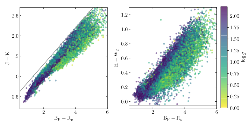
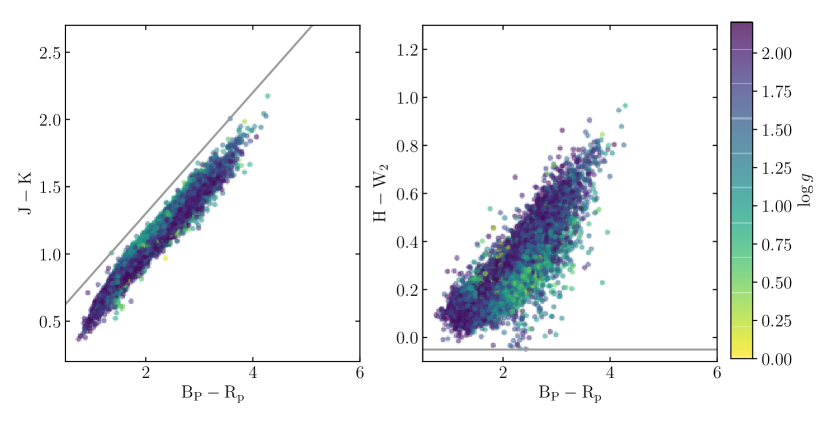
Figure 1: top: Color–color diagrams for the 44784 Parent Sample stars. The points are colored by the APOGEE pipeline estimates of surface gravity. The color cuts used to trim outliers are shown as grey lines. bottom: The same but for the 28226 Training Set stars. Note that there is less color range in the Training Set than in the Parent Sample.

Every Parent Sample star gets, in addition, a randomly assigned binary label (A or B). This is used for two-fold validation and jackknife. In short, we will use the model trained on the Training Set A data to assign spectrophotometric parallaxes to the Parent Sample B data and use the model trained on the Training Set B data to assign spectrophotometric parallaxes to the Parent Sample A data.

For training, we need A and B Training Sets. We define the Training Set stars to be Parent Sample stars that also have a measured Gaia parallax. The Training Set stars, in addition to meeting all Parent Sample cuts, also must meet an uncertainty criterion ${\sigma^{(\mathrm{a})}}_{n}<0.1\,\mathrm{mas}$, i.e.

parallax_error < 0.1 (8)

it must be observed by more than $8$ (widely separated) times

visibility_periods_used >= 8 (9)

as well as meet the additional quality criterion

astrometric_chi2_al / sqrt(astrometric_n_good_obs_al - 5) <= 35 (10)

which eliminates detections that are not consistent with a single PSF (see Bailer-Jones et al., 2018), to ensure that the parallax measurements are good. These cuts leave 28226 stars total in the Training Sets. But—as we have emphasized above—we do not cut ever on parallax or or the ratio to its uncertainty. For this reason, most of the Training Set stars do not have significantly measured parallaxes and more than 2 percent even have negative parallaxes! But we will perform our training such that it will be unbiased in these circumstances. Indeed it would be necessarily biased if ever we did cut on parallax or parallax signal-to-noise.

In detail, for each star $n$ in the Training Sets, we take from Gaia DR2 (Gaia Collaboration et al. 2018) the astrometric parallax ${\varpi^{(\mathrm{a})}}_{n}$ and its uncertainty ${\sigma^{(\mathrm{a})}}_{n}$. Importantly, to each Gaia parallax measurement we add a positive offset $\varpi_{0}$ to adjust for the under-estimation of parallaxes reported by the Gaia Collaboration (Lindegren et al. 2018). The Gaia recommended all-sky-average value is $\varpi_{0}=0.029$ mas (Lindegren et al. 2018), but we adopt $\varpi_{0}=0.048$ mas because that value optimizes our cross-validation objective. It also happens to be in the range of other values found in the literature (Arenou et al. 2018; Zinn et al. 2018). Of course we really expect the offset to be a function of sky position and color (at least), so the offset we find is not recommended for further use as any kind of universal value. The spectrophotometric parallaxes we generate do not depend strongly on this choice, except for small differences at very small parallax (large distance). The Training Sets are shown in the bottom panels of Figure 1.

Comparison of the top and bottom panels of Figure 1 shows that there is more color range in the Parent Sample than in the Training Set. This challenges the representativeness assumption in Section 2. The principal reason for the difference is that the Gaia quality cuts exclude stars preferentially from crowded regions, which also tend to be the most dust-obscured. The hope of the model assumptions is that the Training Set will contain sufficient dust variation that the model will naturally learn the dust corrections and extrapolate acceptably.

For every star $n$ in the full Parent Sample we construct the feature vector $x_{n}$ as

$$x_{n}^{\mathsf{T}} \equiv [1,G_{n},{G_{\mathrm{BP}}}_{n},{G_{\mathrm{RP}}}_{n},J_{n},H_{n},K_{n},W_{1n},W_{2n},\ln f_{1n},\ln f_{2n},\cdots,\ln f_{Ln}]$$ (11)

where the 1 permits a linear offset, the photometry is from Gaia, 2MASS, and WISE, respectively, the fluxes in the $L=7405$ APOGEE spectral pixels (for which there are reliably and consistently data) for star $n$ are denoted $f_{1n}$, $f_{2n}$, and so on, and we have taken logarithms of those fluxes. These feature vectors live in a $D$-dimensional space where $D=7414$. For every star $n$ in either of the Training Sets we additionally require—in addition to these feature vectors—a Gaia-measured astrometric parallax ${\varpi^{(\mathrm{a})}}_{n}$ and uncertainty ${\sigma^{(\mathrm{a})}}_{n}$.

Section 5 Results and validation

We optimize two models, one for Training Set A and one for Training Set B. The two models are applied to the two splits of the Parent Sample, Parent Sample A and Parent Sample B, using the A-trained model on Parent Sample B and vice versa. For the purposes of assessing the accuracy and precision of the model, this train-and-test framework constitutes a two-fold cross-validation. Results of this cross-validation are shown in Figure 2. For the stars with highest Gaia-measured parallax signal-to-noise, the spectrophotometric model is predicting the Gaia parallaxes with little bias and a scatter of less than 9 percent.

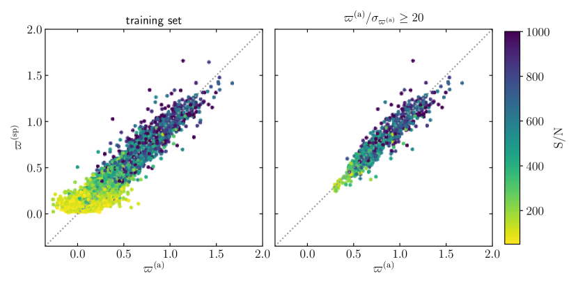
Figure 2: The predictive accuracy of the model, in the two-fold cross-validation. Each panel shows Gaia astrometric parallaxes ${\varpi^{(\mathrm{a})}}_{n}$ on the vertical axis and our spectrophotometric parallaxes ${\varpi^{(\mathrm{sp})}}$ on the horizontal axis. The left panel shows the full Training Set (both A and B combined), and the right panel shows a subset of stars with very high astrometric parallax signal-to-noise. This latter set plays no particular role in the method, but it can be used to demonstrate or assess the prediction precision. The fractional precision of the prediction in the right panel is better than 9 percent. Note that by construction, there can be no negative spectrophotometric parallaxes; that is, the quantity plotted on the vertical axis is positive-definite.

We used this cross-validation framework to adjust the regularization parameter $\Lambda$. A coarse grid search in the value for the spectral-component value of the $\lambda$ vector, using the A/B split as the two-fold cross-validation, with the objective of the cross validation being prediction accuracy. We get a prediction accuracy of better than 9 percent at the optimal setting of the regularization strength.

This 9-percent precision estimate is conservative in the sense that it does not deconvolve or correct for the contributions from the Gaia noise. However, this test is performed with Gaia’s best stars, which are bright, nearby, in low extinction regions, and (because of these things) near Solar metallicity. There could in principle be additional bias or scatter for stars that are in dustier regions or at lower metallicities. Figure 3 shows that there is no suggestion of any such trends when we color the residuals by metallicity or $H-W_{2}$ color (which is a reddening proxy). However, that figure does show that stars with greater reddening do appear to have larger scatter against the Gaia parallaxes. Additional tests confirm that our spectrophotometric parallaxes have largest scatter in the dustiest and most crowded regions, as expected given the relatively low angular resolution photometry.

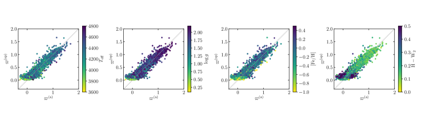
Figure 3: Prediction validation colored by relevant features. Each panel shows the predicted parallax vs the spectrophotometric parallax colored by a different data feature that might be relevant to the residual. Again the quantity plotted on vertical axis is positive-definite.

Another validation of the results can be obtained by looking at known clusters or spatially compact objects in the data. In Figure 4, we show the parallax distribution from Gaia and the spectrophotometric-parallax distribution from our model for stars that are astrometrically confirmed members of three of the stellar clusters in which we validated our results. The cluster members were found by hand, looking at sky and proper-motion distributions centered on literature values. In each case we are plotting only very securely identified cluster members; that is, membership is conservative. We chose the three displayed clusters to span some range in metallicity and age and extinction, and therefore test the accuracy of the method for different kinds of populations. With the exception of M71, the clusters we tested indicate that both Gaia and the spectrophotometric parallaxes appear to be unbiased for these clusters and the range in abundances and ages they represent. The case of cluster M71 is troubling, but after searching for trends with housekeeping data (also see Figure 3) we don’t find any correlations with parallax offsets, although M71 is a higher-extinction cluster.

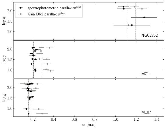
Figure 4: The Gaia astrometric parallaxes ${\varpi^{(\mathrm{a})}}_{n}$ and spectrophotometric parallaxes ${\varpi^{(\mathrm{sp})}}_{n}$ for member stars for three of the stellar clusters in the APOGEE observing footprint. The spectrophotometric parallaxes and their inverse-variance-weighted mean and the astrometric parallaxes and their inverse-variance-weighted mean are shown as vertical lines. Cluster members were identified to be close to the cluster in celestial coordinates and comoving in proper motion.

It is interesting and valuable to compare the spectrophotometric parallax precision to the astrometric parallax precision. Figure 5 compares uncertainties between the spectrophotometric outputs and the astrometric inputs (and recall that information is proportional to the inverse square of the uncertainty). The brief summary is that the spectrophotometric parallaxes are more precise (and even far more precise) than the astrometric parallaxes for stars further than a few kpc from the Sun. This is not unexpected; Gaia parallax uncertainties are in the 0.1-mas range, whereas our uncertainties are in the ten-percent range.

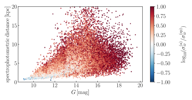
Figure 5: Comparison of precisions between the spectrophotometric parallaxes and the photometric parallaxes, as a function of magnitude and heliocentric distance. Note that the spectrophotometric estimates are more precise for most stars. The information content of a parallax estimate (or any measurement) is proportional to the inverse-square of the uncertainty.

In the end, this method produces a spectrophotometric parallax estimate ${\varpi^{(\mathrm{sp})}}_{m}$ and uncertainty ${\sigma^{(\mathrm{sp})}}_{m}$ for every star $m$. Table 1 shows a snippet of this catalog of output, with the full catalog available as an electronic data table associated with this Article. In order to use this output with Gaia astrometry, we recommend joining our catalog to the Gaia Catalog on the 2MASS ID (name), as per the instructions at the Gaia Archive (Mora et al. 2018). In order to use this output with APOGEE radial velocities and element abundances, we recommend joining our catalog to the SDSS-IV Catalog on the 2MASS ID (name). In addition to this catalog, all the code used for this project is available online in an associated code repository.

Section 6 Discussion

We have demonstrated that photometry and spectroscopy can be used to predict or estimate distances to stars. This isn’t new! However, what’s new is that it is possible to do this very well for luminous giants with unknown ages, and with a purely linear model acting on magnitudes and spectral (logarithmic) fluxes, and entirely data-driven. That is, a linear model trained on noisy parallax data from Gaia.

The model and method are based on a raft of assumptions, listed above in Section 2. We make some comments there, but we emphasize some particulars here:

One strong assumption of this work is that our set of features is sufficient to build a predictive model for distance. Our argument for our included features is that they ought to be sufficient to estimate a dust-independent apparent magnitude and the stellar parameters (especially age and surface gravity) that are sensitive to luminosity. In particular, since our model is linear in the logarithm of the parallax, it is also linear in any kind of apparent magnitude at fixed distance and also linear in distance modulus at fixed luminosity. Our feature decisions were highly motivated by these kinds of considerations.

However, our choice of features is very rigid: In principle the data themselves should tell us what features to include. In that direction, it would make sense to choose features using a more complex technique like deep learning or an auto-encoder. These methods generate good features automatically. They also involve an enormous set of hyper-parameter-like choices, and they involve sacrificing certain kinds of interpretability. All that said, we expect that a better set of features would do better; in this sense the project here is just a first step towards precise spectrophotometric distance estimates.

As we said above, we required that the parallax prediction be constructed from a linear combination of the input data or feature vector components. This may seem like an absurd simplification; it begs the questions: Why did it work? And could we have done better? The answer to the first is that we have taken such a small part of stellar parameter space with our surface-gravity cut, that the linearized model of stellar spectrophotometry is not a bad approximation. Also, because our linear model included photometry in magnitudes (that is, logarithmic) and was exponentiated to make the parallax prediction, we knew in advance that much of the needed flexibility (for dust attenuation, for example) would be close to linear. That is, it was a combination of limited model scope and some cleverness in the feature engineering and model structure.

The answer to the second question is that almost certainly we could have done better! Since models like Gaussian processes and deep networks subsume the linear model (at least approximately), they could have delivered better—or at least non-worse—results. The issues with going to a much more complex model are manifold, however: We would have had many more decisions to make and many more hyper-parameters to set. We would have used some (or maybe much) of the information in the data to learn the simple fact that the problem is close to linear; that is, if you give a model a lot of freedom or capacity, it has to use a lot of the data to learn what part of that capacity it really needs. A more complex model might have had edge issues: Very flexible models don’t extrapolate outside the convex hull of their training data, and our training data was not balanced in terms of parallax and dust attenuation. In the linear model it is also—unlike in more flexible models—trivial to propagate uncertainties from the feature space to the prediction. We used that, above, to propagate uncertainty in equation (5). And finally—in principle—linear models are better for visualization and interpretation; the linear model contains essentially only first derivatives in the data space, which are relatively easy to understand.

Another advantage of a linear model over more general methods (like deep learning, say), is that it is possible to look inside the linear model and check whether the dependencies represented there make sense. For example, the feature vector $x_{n}$ for star $n$ contains a set of photometry in magnitudes. Linear combinations of these photometric measurements are like complex synthetic magnitudes or colors. Similarly, linear combinations of spectral pixels are like a projection of the spectral space. Brief inspection of these linear combinations showed them to be sensible, but it is out of scope here to interpret them in detail.

Although the model, training, and prediction make no use whatsoever of stellar models, we did use stellar models indirectly to select the Parent Sample of stars: We used the APOGEE pipeline (García Pérez et al. 2016) surface-gravity $\log g$ measurements. This tiny use of stellar models could have been obviated by selecting stars not on the basis of the derived physical parameter, but instead selecting stars to be similar, observationally, in the spectral space. That would have lead to a clean sample and made the project independent completely of stellar models.

Our uncertainty estimation is very naive; it presumes that the features are measured with no intrinsic correlations (probably not true for neighboring pixels in the APOGEE spectra, for example) and it does not allow for any biases in the feature inputs. What’s shown in Figure 3 is that the biggest deviations are for stars with large (red) $H-W_{2}$ colors. These are in dusty and crowded regions; we expect that is the crowding that’s causing the greatest problem, because both Gaia and WISE (and probably also 2MASS) photometry is affected by overlapping and blended sources.

We validated the uncertainty estimates by looking at the chi-squared statistic and robust variations of it. We find that chi-squared is larger than expected if the errors are treated naively. However, robust estimates show that this is driven by outliers; median absolute differences are consistent with our expectations under this very naive noise model. We also find that the outliers that drive up the chi-squared statistic tend to be red in $H-W_{2}$.

Figure 4 suggests that there may be some hidden biases in the results; the cluster M71 looks inconsistent between the Gaia and the spectrophotometric parallaxes. We have looked at colors, sky position, and cluster properties, and we don’t have any simple explanation for the discrepancy. This is left as a caveat for the reader and our users.

Because of our train-and-test framework, each star is given a spectrophotometric parallax based on coefficients derived from training on a complementary Training Set sample, of which that star is not a member. This framework ensures that the Gaia parallax ${\varpi^{(\mathrm{a})}}_{m}$ of star $m$ is never used, even indirectly, in generating the spectrophotometric parallax ${\varpi^{(\mathrm{sp})}}_{m}$ of star $m$. That means that the parallax estimates generated here and given in Table 1 are statistically independent of the Gaia parallaxes and can be combined with them in naïve ways, for example in inverse-variance-weighted averages.

This Article and project delivers greatly improved distance estimates for luminous red-giant stars, more luminous than the red clump. The purpose of all this is to make global maps of the Milky Way. Just as a demonstration, we show kinematics and element abundances for stars as a function of position in the Milky Way disk in Figure 6. In this visualization, it is possible to see the rotation of the disk and the kinematic center of the Galaxy; that might even provide a distance estimate to the Galactic Center. It also shows extremely strong chemical gradients.

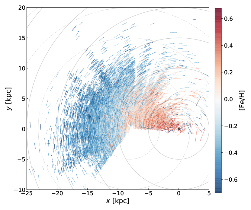
Figure 6: A map of the kinematics and element abundances in the Milky Way disk. Each arrow represents the three-space Galactocentric velocity of each star in the sample, projected onto the Galactic disk plane. To make these velocities, raw Gaia proper motions and APOGEE radial velocities were used (in a standard Galactocentric transformation), so they are not in any way noise-deconvolved. Each arrow has a color corresponding to the APOGEE reported metallicity. This map shows the rotation of the Galaxy out to large radius, and also indicates the kinematic center of the disk rotation. The stars shown in this map have distance uncertainties on the order of ten percent, so at significant heliocentric distances, the interpretation of the quantitative information in this plot requires care.

In a companion paper (Eilers et al. 2018), we are using this information to estimate the (asymmetric-drift-corrected) circular-velocity curve for the Milky Way.

Finally, one comment on the use of these spectrophotometric parallaxes. They are noisy. Precise use of these involves building a likelihood function and performing inference, just as the precise use of the Gaia data presented here required the same. We recommend making analogous inferences when using these outputs.

Table 1: The generated spectrophotometric parallaxes and their uncertainties.. This Table is just a snippet; the full catalog of all 44784 objects in the combined Parent Samples is available online. In order to reproduce the Figures in this Article, this catalog should be joined to the Gaia, 2MASS, WISE  and APOGEE Catalogs by 2MASS ID.

2MASS_ID	Gaia_parallax	Gaia_parallax_err	spec_parallax	spec_parallax_err	training_set	sample
2M00000002+7417074	0.3191	0.0329	0.3185	0.0164	0	B
2M00000317+5821383	0.3643	0.0510	0.4428	0.0183	0	A
2M00000546+6152107	0.3154	0.0351	0.3292	0.0164	0	B
2M00000797+6436119	0.0771	0.0841	0.1943	0.0194	1	B
2M00001719+6221324	0.1395	0.0439	0.1564	0.0128	0	B
2M00002005+5703467	0.3003	0.0247	0.2372	0.0203	0	B
2M00002036+6153416	0.0657	0.0637	0.1347	0.0131	1	A
2M00002118+6136420	0.1936	0.0323	0.2173	0.0133	1	B
2M00002227+6223341	0.1965	0.0450	0.1461	0.0089	0	B
2M00002472+5518473	0.0947	0.0207	0.1473	0.0096	1	B
2M00002908+6140446	0.1675	0.0460	0.1914	0.0176	1	A
2M00003061+5820590	0.1669	0.0339	0.3502	0.0290	1	A
…	…	…	…	…	…	…

Note. — All floating-point numbers are angles in mas.

References

- Abolfathi et al. (2018) Abolfathi, B., Aguado, D. S., Aguilar, G., et al. 2018, ApJS, 235, 42
- Allende Prieto et al. (2008) Allende Prieto, C., Majewski, S. R., Schiavon, R., et al. 2008, Astronomische Nachrichten, 329, 1018
- Arenou et al. (2018) Arenou, F., Luri, X., Babusiaux, C., et al. 2018, A&A, 616, A17
- Astropy Collaboration et al. (2013) Astropy Collaboration, Robitaille, T. P., Tollerud, E. J., et al. 2013, A&A, 558, A33
- Astropy Collaboration et al. (2018) The Astropy Collaboration, Price-Whelan, A. M., Sipőcz, B. M., et al. 2018, arXiv:1801.02634
- Bailer-Jones et al. (2018) Bailer-Jones, C. A. L., Rybizki, J., Fouesneau, M., Mantelet, G., & Andrae, R. 2018, AJ, 156, 58
- Blanton et al. (2017) Blanton, M. R., Bershady, M. A., Abolfathi, B., et al. 2017, AJ, 154, 28
- Byrd et al. (1995) Byrd, R. H., Lu, P., Nocedal, J., & Zhu, C. 1995, SIAM J. Sci. Comput., 16, 1190
- Casey et al. (2016) Casey, A. R., Hogg, D. W., Ness, M., et al. 2016, arXiv:1603.03040
- Eilers et al. (2018) Eilers, A. C., Hogg, D. W., Rix, H.-W., & Ness, M. 2018, in preparation
- Gaia Collaboration et al. (2016) Gaia Collaboration, Prusti, T., de Bruijne, J. H. J., et al. 2016, A&A, 595, A1
- Gaia Collaboration et al. (2018) Gaia Collaboration, Brown, A. G. A., Vallenari, A., et al. 2018, arXiv:1804.09365
- García Pérez et al. (2016) García Pérez, A. E., Allende Prieto, C., Holtzman, J. A., et al. 2016, AJ, 151, 144
- Helmi et al. (2018) Helmi, A., Babusiaux, C., Koppelman, H. H., et al. 2018, arXiv:1806.06038
- Ho et al. (2017) Ho, A. Y. Q., Ness, M. K., Hogg, D. W., et al. 2017, ApJ, 836, 5
- Hogg (2018) Hogg, D. W. 2018, arXiv:1804.07766
- Hunter (2007) Hunter, J. D. 2007, CISE, 9(3), 90
- Jones et al. (2001) Jones, E., Oliphant, E., Peterson, P. et al. 2001, http://www.scipy.org/
- Kollmeier et al. (2017) Kollmeier, J. A., Zasowski, G., Rix, H.-W., et al. 2017, arXiv:1711.03234
- Lindegren et al. (2018) Lindegren, L., Hernandez, J., Bombrun, A., et al. 2018, arXiv:1804.09366
- Lutz & Kelker (1973) Lutz, T. E., & Kelker, D. H. 1973, PASP, 85, 573
- Majewski et al. (2017) Majewski, S. R., Schiavon, R. P., Frinchaboy, P. M., et al. 2017, AJ, 154, 94
- Marrese et al. (2018) Marrase, P. M. et al. 2018, in preparation
- Martig et al. (2016) Martig, M., Fouesneau, M., Rix, H.-W., et al. 2016, MNRAS, 456, 3655
- Mora et al. (2018) Mora, A., González-Núñez, J., Baines, D., et al. 2018, IAU Symposium, 330, 35
- Ness et al. (2015) Ness, M., Hogg, D. W., Rix, H.-W., Ho, A. Y. Q., & Zasowski, G. 2015, ApJ, 808, 16
- Ness et al. (2016) Ness, M., Hogg, D. W., Rix, H.-W., et al. 2016, ApJ, 823, 114
- Ness et al. (2018) Ness, M., Rix, H.-W., Hogg, D. W., et al. 2018, ApJ, 853, 198
- Oliphant (2006) Oliphant, T. E. 2006, A guide to NumPy, Trelgol Publishing
- Pérez & Granger (2007) Pérez, F. & Granger, B. E. 2007, CISE, 9(3), 29
- Skrutskie et al. (2006) Skrutskie, M. F., Cutri, R. M., Stiening, R., et al. 2006, AJ, 131, 1163
- Trick et al. (2018) Trick, W. H., Coronado, J., & Rix, H.-W. 2018, arXiv:1805.03653
- Wilson et al. (2010) Wilson, J. C., Hearty, F., Skrutskie, M. F., et al. 2010, Proc. SPIE, 7735, 77351C
- Wright et al. (2010) Wright, E. L., Eisenhardt, P. R. M., Mainzer, A. K., et al. 2010, AJ, 140, 1868
- Zinn et al. (2018) Zinn, J. C., Pinsonneault, M. H., Huber, D., & Stello, D. 2018, arXiv:1805.02650