Precision Predictions at N³LO for the Higgs Boson Rapidity Distribution at the LHC

Abstract

We present precise predictions for the Higgs boson rapidity distribution at the LHC in the gluon fusion production mode. Our approach relies on the fully analytic computation of six terms in a systematic expansion of the partonic differential cross section around the production threshold of the Higgs boson at next-to-next-to-next-to leading order (N³LO) in QCD perturbation theory. We observe a mild correction compared to the previous perturbative order and a significant reduction of the dependence of the cross section on the perturbative scale throughout the entire rapidity range.

The precision study of the Higgs boson is key to the current and future physics program at the LHC. This is reflected by the remarkable accomplishments Aaboud et al. (2018); Sirunyan et al. (2018) of the ATLAS and CMS experiment that continue to test the interactions of the Higgs boson after its discovery Aad et al. (2012); Chatrchyan et al. (2012). The resulting precise determination of the couplings of the Higgs boson to standard model (SM) particles promises to be a crucial test of physics beyond the SM, especially in absence of direct observations of new particles at the LHC. Our capability to observe small deviations from SM couplings provides key information to test many models that address problems in high energy physics, such as the origin and nature of dark matter. Particularly, in the advent of the high luminosity phase of the LHC it is paramount that the experimental precision is met or surpassed by theoretical predictions in order to reap the full benefit of LHC measurements.

The dominant mechanism for the production of a Higgs boson at the LHC is described by the fusion of two gluons, resolved from the incoming protons, into a virtual top quark loop that then radiates the Higgs boson. Naturally, there is a significant effort by the particle physics community to determine this particular production mode with utmost precision. It has long been known that the gluon fusion cross section is afflicted by particularly large perturbative Quantum Chromodynamics (pQCD) corrections Dawson (1991); Graudenz et al. (1993); Spira et al. (1995); Djouadi et al. (1991); Anastasiou and Melnikov (2002); Harlander and Kilgore (2002); Ravindran et al. (2003). This has motivated a long running program to compute higher order QCD corrections to the inclusive gluon fusion cross section that culminated in the recent determination of the next-to-next-to-next-to leading order (N³LO) corrections in pQCD Anastasiou et al. (2013a, b); Anastasiou et al. (2014); Anastasiou et al. (2015a); Dulat and Mistlberger (2014); Anastasiou et al. (2015b, c); Anastasiou et al. (2016); Dulat et al. (2018a); Mistlberger (2018). Taking into account effects due to the neglected quark masses as well as electro-weak corrections and appraising residual uncertainties from missing higher order effects, the current state-of-the-art prediction for the Higgs production cross section in gluon fusion was obtained in Anastasiou et al. (2016); Dulat et al. (2018a).

Due to the astounding experimental progress we are able to go beyond the determination of total rates and ask more detailed questions about the nature of the Higgs boson. In particular, it is possible to perform measurements differential in kinematic variables such as the transverse momentum or rapidity of the Higgs boson. Currently, precise predictions through next-to-next-to leading order (NNLO) in QCD are available not only for differential Higgs boson observables but also for observables where a Higgs boson is produced in association with a jet Boughezal et al. (2015); Chen et al. (2016, 2018).

In this letter we report the calculation of the Higgs boson rapidity distribution at N³LO in QCD perturbation theory. The rapidity distribution is the only observable that receives genuine corrections at N³LO that are beyond the formal accuracy of cross sections at NNLO for the production of a Higgs boson in association with a jet. Our calculation of this observable relies on an approximation of N³LO matrix elements by means of an expansion around the production threshold of the Higgs boson. This drastically simplifies the calculation of the amplitudes contributing to the N³LO cross section and was already successfully used in the calculation of the inclusive corrections to Higgs boson production at N³LO Anastasiou et al. (2013a, b); Anastasiou et al. (2014); Anastasiou et al. (2015a); Dulat and Mistlberger (2014); Anastasiou et al. (2015b, c); Anastasiou et al. (2016). Additionally, we work in an effective theory (EFT) where the top quark is considered to be infinitely heavy and its degrees of freedom are integrated out. Recently, in ref. Cieri et al. (2018), the rapidity distribution for Higgs production was also approximated at N³LO in the formalism of $q_{T}$-subtraction Catani and Grazzini (2007), exploiting the assumption that one of the ingredients (the third order collinear function) is uniform over the entire rapidity range.

I Set-Up

In collinear factorisation, the probability to produce a Higgs boson with a given rapidity $Y$ can be expressed as

$$\frac{d\sigma_{P\,P\rightarrow H+X}}{dY}=\hat{\sigma}_{0}\sum_{i,j}\int_{0}^{1}dx_{1}dx_{2}dy_{1}dy_{2}f_{i}(y_{1})f_{j}(y_{2})$$

$$\times\delta(\tau-x_{1}x_{2}y_{1}y_{2})\delta\left(Y-\frac{1}{2}\log\left(\frac{x_{1}y_{1}}{x_{2}y_{2}}\right)\right)\eta_{ij}(x_{1},x_{2}).\hskip 14.22636pt$$ (1)

Here, $f_{i}(y)$ are parton distribution functions (PDFs) and $\eta_{ij}(x_{1},x_{2})$ are the partonic coefficient functions (PCFs). The sum runs over all possible combinations of initial state partons and we integrate over the energy fraction of the incoming partons $y_{1/2}$. Furthermore, we define $\tau=m_{h}^{2}/S$ and $S=(P_{1}+P_{2})^{2}$ where the $P_{i}$ are the momenta of the incoming protons and $m_{h}$ is the Higgs boson mass. We factor out the leading order partonic cross section $\hat{\sigma}_{0}$.

The main result of our calculation is the analytic determination of the PCFs in pQCD through N³LO.

$$\eta_{ij}(x_{1},x_{2})=\sum\limits_{i=0}^{3}\left(\frac{\alpha_{S}}{\pi}\right)^{i}\eta_{ij}^{(i)}(x_{1},x_{2})+\mathcal{O}(\alpha_{S}^{4}).$$ (2)

We employ the heavy top quark effective theory which allows us to work only with massless partons and couple the Higgs bosons directly to gluons via an effective interaction. The required Wilson coefficient, matching the EFT to full QCD, was computed in refs. Chetyrkin et al. (1998); Schroder and Steinhauser (2006); Chetyrkin et al. (2006); Kramer et al. (1998); Gerlach et al. (2018). The PCFs are comprised of squared partonic matrix elements with up to three unresolved partons in the final state integrated over the available phase space. The matrix elements through NNLO are known Gehrmann-De Ridder et al. (2012), but we recompute them using our methodology. The purely virtual matrix elements and matrix elements with one additional parton in the final state were computed in refs. Baikov et al. (2009); Gehrmann et al. (2010); Duhr et al. (2015); Gehrmann et al. (2012) and we re-derive them for the purpose of this article. Our computation is performed in the framework of dimensional regularisation in the $\overline{\text{MS}}$ scheme and we rely on previously computed splitting functions Moch et al. (2004); Vogt et al. (2004) and $\beta$-function coefficients van Ritbergen et al. (1997); Czakon (2005); Baikov et al. ; Herzog et al. (2017) to absorb initial state infrared singularities by a standard mass factorisation redefinition of our PDFs and to perform ultra-violet renormalisation. Our main result relies on a suitable approximation of squared matrix elements with two and three partons in the final state which we discuss below.

II Threshold Expansion

The probability to produce a Higgs boson via gluon fusion at the LHC is strongly correlated with the probability to find a pair of gluons in the colliding protons. This gluon luminosity is steeply falling with the center-of-mass energy $s$ of the gluon pair. This results in an enhancement of the hadronic cross section, when the Higgs boson is produced close to threshold, i.e. when $s$ equals the mass of the Higgs boson. This kinematic enhancement was exploited successfully in the past to perform precise approximations of the inclusive Higgs boson production cross section in terms of a systematic expansions around the production threshold Harlander and Kilgore (2002); Anastasiou et al. (2015c). In this limit the threshold parameter $z=m_{h}^{2}/s=x_{1}x_{2}$ tends to one and an expansion can be performed around $\bar{z}=1-z=0$.

In ref. Dulat et al. (2018b) we demonstrated that the rapidity distribution at NNLO can be approximated to a high degree of precision using a threshold expansion. Furthermore, we already obtained the first two terms in the threshold expansion of the PCFs at N³LO. In this article we go beyond this result and obtain in total the first six terms of the expansion in $\bar{z}$. We achieve this by following the strategies outlined in ref. Dulat et al. (2018b) based on integrand expansions of Higgs differential cross sections Dulat et al. (2017); Anastasiou et al. (2013b, 2015b, a), which generalise the techniques employed at NNLO Anastasiou et al. (2003a, b); Anastasiou et al. (2004). The result is a PCF differential in the transverse momentum and rapidity of the Higgs boson. In order to obtain our $\eta_{ij}^{(3)}(x_{1},x_{2})$ we analytically integrate out the extra degree of freedom corresponding to the transverse momentum.

In the variables $x_{1}$ and $x_{2}$ the threshold expansion can be performed by introducing a formal expansion parameter $\delta$ such that

$$\bar{x}_{1}\rightarrow\delta\bar{x}_{1}\frac{1-\bar{x}_{2}}{1-\delta\bar{x}_{2}},\hskip 14.22636pt\bar{x}_{2}\rightarrow\delta\bar{x}_{2}.$$ (3)

Here, $\bar{x}_{i}=1-x_{i}$. The expansion parameter $\delta$ is chosen exactly such that each term in the expansion around $\delta=0$ of our PCF corresponds exactly to one term in the expansion in $\bar{z}$.

III Exploiting the Divergence Structure

The bare PCFs at N³LO, arising from the calculation of contributing squared matrix elements, in $d=4-2\epsilon$ dimensions take the form

$$\eta_{ij,\,\text{bare}}^{(3)}(\bar{x}_{1},\bar{x}_{2}) = \eta_{ij,\,\text{virt.}}^{(3)}\delta(\bar{x}_{1})\delta(\bar{x}_{2})$$

$$+ \sum_{n,m=1}^{3}\bar{x}_{1}^{-1-m\epsilon}\bar{x}_{2}^{-1-n\epsilon}\eta_{ij,\,\text{bare}}^{(3,m,n)}(\bar{x}_{1},\bar{x}_{2}).$$

The term $\eta_{ij,\,\text{virt.}}^{(3)}\delta(\bar{x}_{1})\delta(\bar{x}_{2})$ corresponds to the purely virtual contributions with a leading divergence of $1/\epsilon^{6}$. The functions $\eta_{ij,\,\text{bare}}^{(3,n,m)}(\bar{x}_{1},\bar{x}_{2})$ are holomorphic around $\bar{x}_{i}=0$ and contain fourth order poles in $\epsilon$. In order to expand the PCFs in the dimensional regulator we perform a standard expansion of singular factors in terms of delta functions $\delta(\bar{x}_{i})$ and plus-distributions $\left[L^{n}_{i}/\bar{x}_{i}\right]_{+}$ with $L_{i}=\log(\bar{x}_{i})$.

We obtain our finite, renormalised N³LO coefficient function by combining the bare PCF with a suitable mass factorisation and ultraviolet renormalisation counter term $CT^{(3)}_{ij}$. This counter term equally contains distributions and renders the renormalised PCFs finite,

$$\eta_{ij}^{(3)}(x_{1},x_{2}) = \lim\limits_{\epsilon\rightarrow 0}\left[\eta_{ij,\,\text{bare}}^{(3)}(x_{1},x_{2})+CT^{(3)}_{ij}(x_{1},x_{2})\right]$$ (5)

$$= \sum\limits_{k,l}D_{k}(\bar{x}_{1})D_{l}(\bar{x}_{2})\eta_{ij,(k,l)}^{(3)}(x_{1},x_{2}).$$

In the second line in the above equation we isolate the structures that are singular in the limit $\bar{x}_{i}\to 0$ into the functions $D_{k}(\bar{x}_{i})$ such that the coefficients $\eta_{ij,(k,l)}^{(3)}(x_{1},x_{2})$ are either real numbers or holomorphic functions in the limit. The non-holomorphic function $D_{k}(\bar{x}_{i})$ corresponds to the $k^{th}$ entry of the following list of 12 possible structures that can appear in the cross section through N³LO,

$$\left\{\delta(\bar{x}_{i}),\left[\frac{L^{0}_{i}}{\bar{x}_{i}}\right]_{+},\dots,\left[\frac{L^{5}_{i}}{\bar{x}_{i}}\right]_{+},L^{0}_{i},\dots L^{4}_{i}\right\}.$$ (6)

The fact that all explicit poles in the dimensional regulator have to cancel among the different contributions in eq. (5), allows us to derive relations among the various bare partonic coefficients in eq. (III) and the counter term. Using the fact that only the known, genuine two loop contributions can produce bare coefficient functions contributing to the $n=1$ or $m=1$ terms in eq. (III), this becomes a powerful tool to determine many of the coefficients $\eta_{ij,(k,l)}^{(3)}(x_{1},x_{2})$ exactly.

All coefficients of terms proportional to two distributions were already computed in ref. Dulat et al. (2018b) and can also be deduced from the inclusive cross section at threshold (c.f. ref. Anastasiou et al. (2014); Li et al. (2015)) as was done in ref. Ahmed et al. (2014). Furthermore, we observe that if we consider only the leading power term in either one of the $\bar{x}_{i}$, a reduced number of exponents contributes to eq. (III), such that $n\leq m$, which further constrains our system of equations. Using these relations, we were able to determine all coefficients in eq. (5) exactly in $\bar{x}_{i}$, except for the terms,

$$\eta_{ij,\,\text{missing}}^{(3)}(x_{1},x_{2})=\Big{[}\delta(\bar{x}_{1})\log(\bar{x}_{2})\eta_{ij,(1,9)}^{(3)}(0,x_{2})$$ (7)

$$\hskip 14.22636pt+\delta(\bar{x}_{1})\eta_{ij,(1,8)}^{(3)}(0,x_{2})+\left[\frac{1}{\bar{x}_{1}}\right]_{+}\eta_{ij,(2,8)}^{(3)}(0,x_{2})$$

$$\hskip 14.22636pt+\log(\bar{x}_{2})\eta_{ij,(8,9)}^{(3)}(x_{1},x_{2})\Big{]}+\Big{[}(x_{1}\leftrightarrow x_{2})\Big{]}$$

$$\hskip 14.22636pt+\eta_{ij,(8,8)}^{(3)}(x_{1},x_{2})+\log(\bar{x}_{1})\log(\bar{x}_{2})\eta_{ij,(9,9)}^{(3)}(x_{1},x_{2}).$$

While the above terms could not be determined exactly from our current knowledge of unexpanded matrix elements, we obtained them via a threshold expansion as described above. Notice, that the above contributions contain maximally one power of a logarithm that is enhanced as $\bar{x}_{i}\rightarrow 0$.

In our final approximation of the PCF we choose to re-organise the terms without any distributions such that all terms proportional to threshold logarithms $\log^{i}(\bar{z})$ with $i\geq 3$ are maintained exactly. We approximate terms with lower powers of threshold logarithms using the threshold expansion as discussed above. Note, that the relations among the different components of the PCF provide a highly non-trivial consistency check on the results from our threshold expansion.

The partonic coefficient functions also depend explicitly on logarithms of the perturbative scale $\mu$ and we can rearrange them as,

$$\eta_{ij}^{(3)}(x_{1},x_{2})=\sum_{l=0}^{3}\eta_{ij}^{(3,l)}(x_{1},x_{2})\log^{l}\left(\frac{m_{h}^{2}}{\mu^{2}}\right).$$ (8)

Naturally, the functions $\eta_{ij}^{(3,l)}(x_{1},x_{2})$ can be decomposed into distribution-valued or logarithmically enhanced terms as above. However, the coefficients with $l\geq 1$ can be derived exactly from lower order cross sections by solving the DGLAP evolution equations. Consequently, we determine them exactly, with one exception: The derivation of the non-distribution valued, non-logarithmically enhanced term of the coefficient of $\log\left(m_{h}^{2}/\mu^{2}\right)$ involves rather cumbersome convolution integrals. We approximate this particular term using a threshold expansion which modifies our approximation at terms beyond the claimed formal accuracy.

IV Matching to the Inclusive Cross Section

The inclusive PCF for Higgs boson gluon fusion production at N³LO was computed exactly in ref. Mistlberger (2018). It is a one parameter function of the threshold variable $z$. By performing the variable transformation $\{\bar{x}_{1}=\frac{(1-\bar{x})\bar{z}}{1-\bar{x}\bar{z}},\bar{x}_{2}=\bar{x}\bar{z}\}$ we can relate our differential PCF to the inclusive one,

$$\eta_{ij}^{(3),\text{inc.}}(z)=\int_{0}^{1}\frac{\bar{z}d\bar{x}}{(1-\bar{z}\bar{x})}\eta_{ij}^{(3)}\left(\frac{(1-\bar{x})\bar{z}}{1-\bar{x}\bar{z}},\bar{x}\bar{z}\right)\,.$$ (9)

The above relation provides an enormously stringent check on our partonic coefficient functions. Indeed, our threshold expansion agrees with the threshold expansion of the inclusive partonic coefficient function for all computed orders.

Furthermore, eq. (9) allows us to modify our differential partonic coefficient functions by terms of higher order in the threshold expansion such that the exact inclusive cross section is automatically obtained if the integral over the rapidity distribution is performed,

$$\eta_{ij}^{(3),\text{matched}}(x_{1},x_{2})=\eta_{ij}^{(3),\text{app.}}(x_{1},x_{2})$$ (10)

$$\hskip 14.22636pt+\frac{x_{1}+x_{2}}{2(1-x_{1}x_{2})}\left[\eta_{ij}^{(3),\text{inc}}(x_{1}x_{2})-\eta_{ij}^{(3),\text{inc, app.}}(x_{1}x_{2})\right].$$

Here, $\eta_{ij}^{(3),\text{app.}}$ corresponds to the approximation of the PCF obtained as described in the previous sections and $\eta_{ij}^{(3),\text{inc, app.}}$ is its inclusive counterpart obtained by virtue of eq. (9). Furthermore, $\eta_{ij}^{(3),\text{inc}}$ is the inclusive partonic coefficient function obtained in ref. Mistlberger (2018). The term in the square bracket of eq. (10) contains therefore only terms that are higher order in the threshold expansion than those obtained as described above. This modification of the PCF ensures that if the inclusive integral over the Higgs boson rapidity is performed the correct cross section is obtained for each partonic center of mass energy. The approximation derived in eq. (10) will be the basis for our numerical results presented below.

V Phenomenological Results

In the previous sections we derive an analytic approximation to the PCF for the Higgs boson cross section differential in the rapidity through N³LO in QCD. We now use MMHT2014 PDFs Thorne et al. (2015) to derive predictions for hadronic Higgs boson rapidity distribution at the LHC with a centre of mass energy of $13$ TeV by means of eq. (I). We implement our coefficient functions into a private C++ code and use LHAPDF Buckley et al. (2015) to perform the $\mu^{2}$ evolution of the PDF grids and evaluate them with a private grid interpolator. The Cuba library Hahn (2005) is used to perform the numerical integration over the momentum fractions of the partons.

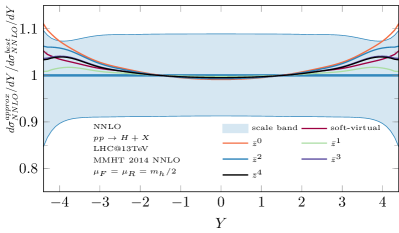
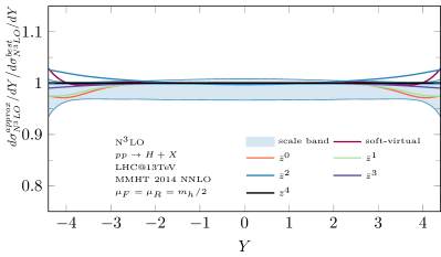
Figure 1: Approximate Higgs boson rapidity distribution with threshold expansion truncated at different orders. The left panel shows the ratio of the approximate NNLO to the exact result, the right panel shows the approximate N³LO result to the best prediction obtained in this work.

As validation, we first derive the NNLO analogue of the approximation of the PCF used at N³LO and show the resulting predictions in the left panel of fig. 1 normalised to the exact rapidity distribution through NNLO with a central scale of $\mu=m_{h}/2$. The blue band corresponds to the cross section obtained by varying the common scale $\mu$ in the interval $[m_{h}/4,m_{h}]$. The coloured lines show the cross section obtained by truncating the threshold expansion in our approximation at different orders. We observe that our approximation describes the NNLO rapidity distribution very well for central rapidities $(|Y|<3)$ and even performs fine for larger rapidities. Deterioration of the threshold approximation at larger rapidities can be expected as on average the final state of the scattering process is more energetic, i.e. further from the production threshold. Including an increasing number of terms systematically improves the approximation. We also observe that all rapidity distributions obtained from truncated threshold expansions fall well within the scale variation band of the exact NNLO cross section.

In the right panel of fig. 1 we show predictions for the N³LO rapidity distribution truncating the threshold expansion at different orders normalised to our best approximation. Similarly to the case at NNLO, including more terms in the expansion systematically stabilises our approximation. Central rapidities are remarkably stable under the inclusion of more and more expansion terms. In particular, all truncated approximations are once again contained within the scale variation band for central rapidities. We explored relaxing some of the ingredients of our approximation (less exact distributions or no matching to the exact inclusive cross section) which amounts to a modification of terms beyond those computed in our threshold expansion and find only slight variation in our prediction. For example, basing our calculation purely on a threshold expansion with six terms, underestimates the inclusive cross section by $0.25\%$ and only slightly varies the shape of the rapidity distribution. Similarly, we checked that a simple reweighting of the threshold-expanded N³LO rapidity distribution to the exact inclusive cross section at N³LO produces results that are very close to our best prediction including the matching procedure according to eq. (9). We observe that at NNLO we approximate the exact PCF to better than one percent for $|Y|<2$ and better than two percent for $|Y|<3$. In order to be conservative we estimate that our prediction is at the same level of precision relative to the exact result at N³LO.

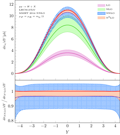
Figure 2: The Higgs boson rapidity distribution at different orders in perturbation theory. The lower panel shows the N³LO and NNLO predictions normalised to the N³LO prediction for $\mu=m_{h}/2$.

In fig. 2 we show the rapidity distribution of the Higgs boson truncated at different orders in QCD perturbation theory. Our newly derived N³LO predictions display a stabilisation of the perturbative series as well as a drastic reduction of the size of perturbative scale dependence. We observe that the ratio of the rapidity distribution at N³LO relative to NNLO is uniform over the entire range of Higgs boson rapidities. Consequently, the N³LO rapidity distribution can be reproduced to very high accuracy by rescaling the NNLO prediction by the inclusive N³LO k-factor. Our findings for the central value and scale variation of the rapidity distribution are in agreement with the result presented in ref. Cieri et al. (2018). At very large rapidities the authors of ref. Cieri et al. (2018) observe a slight deviation from an entirely uniform N³LO correction but our predictions are still compatible within uncertainties.

To conclude, in this article we have obtained theoretical predictions for the Higgs boson rapidity distribution at significantly improved levels of precision. The scale variation of the N³LO cross section for $|Y|<3$ is reduced to $[-3.4\%,+0.9\%]$ and we estimate the uncertainty due to missing higher orders in the threshold expansion to be less than $1\%$ for $|Y|<2$ and less than $2\%$ for $|Y|<3$. Our result has direct implications for the LHC phenomenology program and represents a mile stone in the field of perturbative QCD. We expect the result of this work to be the corner stone of future fully differential Higgs boson phenomenology.

Acknowledgements: We are grateful to Alexander Huss for useful discussions. We thank Babis Anastasiou, Thomas Gehrmann, Stefan Hoeche and Giulia Zanderighi for useful comments on the manuscript. The research of FD is supported by the U.S. Department of Energy (DOE) under contract DE-AC02-76SF00515. AP is supported by the European Commission through the ERC grant pertQCD. BM is supported by the Pappalardo fellowship and was supported by the European Comission through the ERC Consolidator Grant HICCUP (No. 614577).

References

- Aaboud et al. (2018) M. Aaboud et al. (ATLAS), Phys. Lett. B786, 114 (2018), eprint 1805.10197.
- Sirunyan et al. (2018) A. M. Sirunyan et al. (CMS) (2018), eprint 1809.10733.
- Aad et al. (2012) G. Aad, T. Abajyan, B. Abbott, J. Abdallah, S. A. Khalek, A. Abdelalim, O. Abdinov, R. Aben, B. Abi, M. Abolins, et al., Physics Letters B 716, 1 (2012), ISSN 0370-2693, URL http://www.sciencedirect.com/science/article/pii/S037026931200857X.
- Chatrchyan et al. (2012) S. Chatrchyan, V. Khachatryan, A. Sirunyan, A. Tumasyan, W. Adam, E. Aguilo, T. Bergauer, M. Dragicevic, J. Erö, C. Fabjan, et al., Physics Letters B 716, 30 (2012), ISSN 0370-2693, URL http://www.sciencedirect.com/science/article/pii/S0370269312008581.
- Dawson (1991) S. Dawson, Nucl. Phys. B359, 283 (1991).
- Graudenz et al. (1993) D. Graudenz, M. Spira, and P. M. Zerwas, Phys. Rev. Lett. 70, 1372 (1993).
- Spira et al. (1995) M. Spira, A. Djouadi, D. Graudenz, and P. M. Zerwas, Nucl. Phys. B453, 17 (1995), eprint hep-ph/9504378.
- Djouadi et al. (1991) A. Djouadi, M. Spira, and P. M. Zerwas, Phys. Lett. B264, 440 (1991).
- Anastasiou and Melnikov (2002) C. Anastasiou and K. Melnikov, Nuclear Physics B 646, 220 (2002), ISSN 05503213, eprint 0207004, URL http://arxiv.org/abs/hep-ph/0207004.
- Harlander and Kilgore (2002) R. V. Harlander and W. B. Kilgore, Phys. Rev. Lett. 88, 201801 (2002), eprint hep-ph/0201206.
- Ravindran et al. (2003) V. Ravindran, J. Smith, and W. L. van Neerven, Nucl. Phys. B665, 325 (2003), eprint hep-ph/0302135.
- Anastasiou et al. (2013a) C. Anastasiou, C. Duhr, F. Dulat, and B. Mistlberger, p. 78 (2013a), eprint 1302.4379, URL http://arxiv.org/abs/1302.4379.
- Anastasiou et al. (2013b) C. Anastasiou, C. Duhr, F. Dulat, F. Herzog, and B. Mistlberger, JHEP 12, 088 (2013b), eprint 1311.1425.
- Anastasiou et al. (2014) C. Anastasiou, C. Duhr, F. Dulat, E. Furlan, T. Gehrmann, F. Herzog, and B. Mistlberger, Phys. Lett. B737, 325 (2014), eprint 1403.4616.
- Anastasiou et al. (2015a) C. Anastasiou, C. Duhr, F. Dulat, E. Furlan, T. Gehrmann, F. Herzog, and B. Mistlberger, JHEP 03, 091 (2015a), eprint 1411.3584.
- Dulat and Mistlberger (2014) F. Dulat and B. Mistlberger (2014), eprint 1411.3586.
- Anastasiou et al. (2015b) C. Anastasiou, C. Duhr, F. Dulat, E. Furlan, F. Herzog, and B. Mistlberger, JHEP 08, 051 (2015b), eprint 1505.04110.
- Anastasiou et al. (2015c) C. Anastasiou, C. Duhr, F. Dulat, F. Herzog, and B. Mistlberger, Phys. Rev. Lett. 114, 212001 (2015c), eprint 1503.06056.
- Anastasiou et al. (2016) C. Anastasiou, C. Duhr, F. Dulat, E. Furlan, T. Gehrmann, F. Herzog, A. Lazopoulos, and B. Mistlberger, JHEP 05, 058 (2016), eprint 1602.00695.
- Dulat et al. (2018a) F. Dulat, A. Lazopoulos, and B. Mistlberger, Comput. Phys. Commun. 233, 243 (2018a), eprint 1802.00827.
- Mistlberger (2018) B. Mistlberger, JHEP 05, 028 (2018), eprint 1802.00833.
- Boughezal et al. (2015) R. Boughezal, F. Caola, K. Melnikov, F. Petriello, and M. Schulze, Phys. Rev. Lett. 115, 082003 (2015), eprint 1504.07922.
- Chen et al. (2016) X. Chen, J. Cruz-Martinez, T. Gehrmann, E. W. N. Glover, and M. Jaquier, JHEP 10, 066 (2016), eprint 1607.08817.
- Chen et al. (2018) X. Chen, T. Gehrmann, E. W. N. Glover, A. Huss, Y. Li, D. Neill, M. Schulze, I. W. Stewart, and H. X. Zhu (2018), eprint 1805.00736.
- Cieri et al. (2018) L. Cieri, X. Chen, T. Gehrmann, E. W. N. Glover, and A. Huss (2018), eprint 1807.11501.
- Catani and Grazzini (2007) S. Catani and M. Grazzini, Phys. Rev. Lett. 98, 222002 (2007), eprint hep-ph/0703012.
- Chetyrkin et al. (1998) K. G. Chetyrkin, B. A. Kniehl, and M. Steinhauser, Nucl. Phys. B510, 61 (1998), eprint hep-ph/9708255.
- Schroder and Steinhauser (2006) Y. Schroder and M. Steinhauser, JHEP 01, 051 (2006), eprint hep-ph/0512058.
- Chetyrkin et al. (2006) K. Chetyrkin, J. Kühn, and C. Sturm, Nuclear Physics B 744, 121 (2006), ISSN 05503213, URL http://inspirehep.net/record/699609.
- Kramer et al. (1998) M. Kramer, E. Laenen, and M. Spira, Nucl. Phys. B511, 523 (1998), eprint hep-ph/9611272.
- Gerlach et al. (2018) M. Gerlach, F. Herren, and M. Steinhauser (2018), eprint 1809.06787.
- Gehrmann-De Ridder et al. (2012) A. Gehrmann-De Ridder, T. Gehrmann, and M. Ritzmann, JHEP 10, 047 (2012), eprint 1207.5779.
- Baikov et al. (2009) P. A. Baikov, K. G. Chetyrkin, A. V. Smirnov, V. A. Smirnov, and M. Steinhauser, Phys. Rev. Lett. 102, 212002 (2009), eprint 0902.3519.
- Gehrmann et al. (2010) T. Gehrmann, E. W. N. Glover, T. Huber, N. Ikizlerli, and C. Studerus, Journal of High Energy Physics 2010, 94 (2010), ISSN 1029-8479, URL http://link.springer.com/10.1007/JHEP06(2010)094.
- Duhr et al. (2015) C. Duhr, T. Gehrmann, and M. Jaquier, JHEP 02, 077 (2015), eprint 1411.3587.
- Gehrmann et al. (2012) T. Gehrmann, M. Jaquier, E. W. N. Glover, and A. Koukoutsakis, JHEP 02, 056 (2012), eprint 1112.3554.
- Moch et al. (2004) S. Moch, J. Vermaseren, and A. Vogt, Nuclear Physics B 688, 101 (2004), ISSN 05503213, URL http://linkinghub.elsevier.com/retrieve/pii/S0550321304002445.
- Vogt et al. (2004) A. Vogt, S. Moch, and J. Vermaseren, Nuclear Physics B 691, 129 (2004), ISSN 05503213, URL http://linkinghub.elsevier.com/retrieve/pii/S0550321304003074.
- van Ritbergen et al. (1997) T. van Ritbergen, J. A. M. Vermaseren, and S. A. Larin, Phys. Lett. B400, 379 (1997), eprint hep-ph/9701390.
- Czakon (2005) M. Czakon, Nucl. Phys. B710, 485 (2005), eprint hep-ph/0411261.
- (41) P. A. Baikov, K. G. Chetyrkin, and J. H. Kühn, Phys. Rev. Lett. 118, 082002 (????), eprint 1606.08659.
- Herzog et al. (2017) F. Herzog, B. Ruijl, T. Ueda, J. A. M. Vermaseren, and A. Vogt, JHEP 02, 090 (2017), eprint 1701.01404.
- Dulat et al. (2018b) F. Dulat, B. Mistlberger, and A. Pelloni, JHEP 01, 145 (2018b), eprint 1710.03016.
- Dulat et al. (2017) F. Dulat, S. Lionetti, B. Mistlberger, A. Pelloni, and C. Specchia, JHEP 07, 017 (2017), eprint 1704.08220.
- Anastasiou et al. (2003a) C. Anastasiou, L. Dixon, and K. Melnikov, Nuclear Physics B - Proceedings Supplements 116, 193 (2003a), ISSN 09205632, URL http://linkinghub.elsevier.com/retrieve/pii/S0920563203801688.
- Anastasiou et al. (2003b) C. Anastasiou, L. Dixon, K. Melnikov, and F. Petriello, Physical Review Letters 91, 182002 (2003b), ISSN 0031-9007, URL http://link.aps.org/doi/10.1103/PhysRevLett.91.182002.
- Anastasiou et al. (2004) C. Anastasiou, L. Dixon, K. Melnikov, and F. Petriello, Physical Review D 69, 094008 (2004), ISSN 1550-7998, URL http://link.aps.org/doi/10.1103/PhysRevD.69.094008.
- Li et al. (2015) Y. Li, A. von Manteuffel, R. M. Schabinger, and H. X. Zhu, Phys. Rev. D91, 036008 (2015), eprint 1412.2771.
- Ahmed et al. (2014) T. Ahmed, M. K. Mandal, N. Rana, and V. Ravindran, Phys. Rev. Lett. 113, 212003 (2014), eprint 1404.6504.
- Thorne et al. (2015) R. Thorne, L. A. Harland-Lang, A. D. Martin, and P. Motylinski, PoS DIS2015, 056 (2015).
- Buckley et al. (2015) A. Buckley, J. Ferrando, S. Lloyd, K. Nordström, B. Page, M. Rüfenacht, M. Schönherr, and G. Watt, Eur. Phys. J. C75, 132 (2015), eprint 1412.7420.
- Hahn (2005) T. Hahn, Comput. Phys. Commun. 168, 78 (2005), eprint hep-ph/0404043.