Constraints on the common-envelope evolution process from wide triple systems

Abstract

Common envelope (CE) is an important phase in the evolution of interacting evolved binary systems. The interaction of the binary components during the CE evolution (CEE) stage gives rise to orbital inspiral and the formation of a short-period binary or a merger, on the expense of extending and/or ejecting the envelope. CEE is not well understood, as hydrodynamical simulations show that only a fraction of the CE-mass is ejected during the dynamical inspiral, in contrast with observations of post-CE binaries. Different CE models suggest different timescales are involved in the CE-ejection, and hence a measurement of the CE-ejection timescale could provide direct constraints on the CEE-process. Here we propose a novel method for constraining the mass-loss timescale of the CE, using post-CE binaries which are part of wide-orbit triple systems. The orbit/existence of a third companion constrains the CE mass-loss timescale, since rapid CE mass-loss may disrupt the triple system, while slower CE mass-loss may change the orbit of the third companion without disrupting it. As first test-cases we examine two observed post-CE binaries in wide triples, Wolf-1130 and GD-319. We follow their evolution due to mass-loss using analytic and numerical tools, and consider different mass-loss functions. We calculate a wide grid of binary parameters and mass-loss timescales in order to determine the most probable mass-loss timescale leading to the observed properties of the systems. We find that mass-loss timescales of the order of $10^{3}-10^{5}{\rm yr}$ are the most likely to explain these systems. Such long timescales are in tension with most of the CE mass-loss models, which predict shorter, dynamical timescales, but are potentially consistent with the longer timescales expected from the dust-driven winds model for CE ejection.

1 Introduction

Common envelope evolution (CEE) is a relatively short binary evolution phase, typically thought to occur on up to a few dynamical timescales. It occurs when two stars orbit their center of mass in a shared CE . CEE was first suggested by Paczynski (1976) and van den Heuvel (1976) in order to explain the observations of short period (<days) binaries with a degenerate component, now known as post-CE binaries. The degenerate component in the binary must have been much greater in size than the observed separation between the stars of the binary. Hence it was suggested that both stars shared the large envelope of an evolved star, and the dissipative interaction with the CE lead to the CE-ejection and the inspiral of the binary into short-period, or even lead to its merger.

The driving engine of CE-ejection is still debated, and several competing models were suggested (e.g. see Ivanova et al. 2013 for a review, see Glanz & Perets 2018 for a brief overview and updates). Hydrodynamical simulations modeling the dynamical inspiral phase show that only a fraction of the CE-mass is ejected during the inspiral (e.g. Taam & Ricker, 2010; De Marco et al., 2011; Passy et al., 2012; Ivanova et al., 2013) raising a challenge to the simple picture of a dynamical inspiral, and suggesting that additional source of energy are required for the CE-ejection. The timescale for the fractional mass-loss is a few dynamical timescales extending over a few up to a few tens of years. Ivanova and collaborators (Ivanova et al. 2015, and references therein; Clayton et al. 2017, and references therein) suggest that recombination energy from the cooling expanding envelope can provide the necessary source, and their models suggest that the CE-ejection time could be as long as of $10-100{\rm yr}$. Glanz & Perets (2018) suggest that radiation on dust forming in the outer layers of the extended cooling envelope can provide a CE-mechanism similar to that thought to operate in asymptotic giant branch (AGB) stars. In this model the timescale for the CE-ejection is longer, likely $10^{4}-10^{5}{\rm yr}$, and could be comparable to the timescale of AGB mass-loss. In principal, measurement of the CE mass-loss timescale could constrain the different models suggested. However, all of these various timescales are relatively short in comparison with the stellar lifetimes, making the likelihood for direct observations of the ejection small.

Here we propose a novel method to indirectly constrain the CE mass-loss timescales using post-CE binaries which are part of wide triple systems. The existence of a third wide-orbit companion to a post-CE binary, and the orbit properties can potentially constrains the CE mass-loss timescale, since rapid CE mass-loss may disrupt the triple system, while slower CE mass-loss may change the orbit of the third companion without disrupting it. Different mass-loss timescale and mass-loss evolution give rise to different orbital configuration of the systems, and the distribution of such wide triples can potentially constrain CE-mass-loss timescales.

Here we discuss the method and use two observed post-CE binaries in triple systems as test-cases. We consider the two triple systems, Wolf 1130 (Mace et al., 2018) and GD 319 (Farihi et al., 2005); both are post-CE binaries with distant third companions. Given the wide separation (thousands of AU) we can treat outer orbit of the triple system as a wide binary, and consider the inner post-CE binary as a primary single point mass. The evolution and final outcome of the outer-binary is determined by its initial configuration (masses, separation and eccentricity) at the start of the mass loss (Hills, 1983), and the mass-loss evolution.

The paper is organized as follows: in section 2 we discuss the mass-loss dynamics in binary systems, generally divided to three timescale regimes: prompt (fast) mass loss, adiabatic (slow) mass loss and comparable-timescale mass-loss. In section 3 we present the system Wolf 1130 and analyze its possible evolution from the progenitor stage to its current configuration, as to find the most probable mass loss timescale consistent with its currently observed configuration. In section 4 we repeat the analysis for the system GD 319 system. Finally, in section 5 we discuss the results and implications and then summarize (section 6 ).

2 Mass loss in binary systems

The orbital elements (in particular the semi-major axis; SMA, $a$; and eccentricity, $e$) of a gravitationally bound, but otherwise non-interacting binary system are conserved. However, when the binary losses mass the orbital elements may vary in time. We focus on three different regimes, generally divided by ratio of the mass-loss times-scale, $T_{{\rm ML}}$ to the orbital period of the binary, $P_{{\rm binary}}$. These include the prompt mass-loss regime for which $T_{{\rm ML}}/P\ll 1$ discussed in subsection 2.1; the adiabatic mass-loss regime for which $T_{{\rm ML}}/P\gg 1$ discussed in subsection 2.2; and the regime of comparable timescales $T_{{\rm ML}}\sim P$ discussed in subsection 2.3. Throughout the discussion and analysis we assume an overall isotropic mass loss and hence the specific orbital angular momentum is constant; future studies may explore more complex cases. Note the total angular momentum in all of the cases changes due the mass loss.

2.1 Prompt mass loss

Prompt mass loss is defined by the following condition

$$P_{{\rm binary}}\times\dot{M}_{{\rm binary}}\gg M_{{\rm binary}}$$ (1)

where $P_{{\rm binary}}$ is the binary orbital period, $M_{{\rm binary}}$ and $\dot{M}_{{\rm binary}}$ are the binary mass and the binary mass loss respectively. Namely, in the regime of prompt mass loss a significant fraction of the binary mass is ejected on timescales much shorter than the orbital period. This case is relevant for fast events such as supernova explosions or dynamical mass ejection. To first order, in this regime we can approximate the mass loss to be instantaneous.

Many studies explore prompt mass loss (e.g. Blaauw, 1961; Hills, 1983). The ratio of the final SMA of the systems to its initial one in this case is given by (Hills, 1983)

$$\frac{a_{{\rm f}}}{a_{i}}=\frac{1}{2}\left[\frac{M_{{\rm binary}}-\Delta M}{\frac{1}{2}M_{{\rm binary}}-\left(\frac{a_{i}}{r}\right)\Delta M}\right]$$ (2)

where $a_{i}$ and $a_{f}$ are the initial and final SMA respectively, $\Delta M$ is the amount of mass lost from the binary and $r$ is the separation of the components of the binary before the mass loss occurred. An immediate result from (2) is the condition for a binary to survive (i.e. still be bound) following the mass-loss evolution in this regime is

$$\frac{\Delta M}{M_{{\rm binary}}}\leq\frac{r}{2a_{i}}.$$ (3)

Therefore, a circular $\left(r=a_{i}\right)$ binary which loses more than half of its original mass will be disrupted regardless of its initial SMA. For an eccentric orbit the disruption of the binary depends on the separation of the binary at the instantaneous moment of the mass-loss event. The maximal separation for a binary with an eccentric orbit is $r=a_{i}\left(1+e\right)$, and the condition for binary survival is

$$\alpha\leq\frac{1+e}{2}$$ (4)

where $\alpha$ is the fraction of mass lost from the system. Furthermore, the final eccentricity is given by

$$e_{f}=\left\{1-\left(1-e_{i}^{2}\right)\left[\frac{1-\left(\frac{2a_{i}}{r}\right)\left(\frac{\Delta M}{M_{{\rm binary}}}\right)}{\left(1-\frac{\Delta M}{M_{{\rm binary}}}\right)^{2}}\right]\right\}^{1/2}.$$ (5)

2.2 Adiabatic mass loss

Adiabatic mass loss is defined by the following condition:

$$P_{{\rm binary}}\times\dot{M}_{{\rm binary}}\ll M_{{\rm binary}}.$$ (6)

Namely, the amount of mass lost from the system in one orbit is negligible compared to the total mass of the system. In this case, where the mass-loss timescale is much longer than the orbital period we can treat the system with its adiabatic invariant and get the following well known results for the SMA and eccentricity (Jeans, 1961):

$$\frac{a_{f}}{a_{i}}=\frac{M_{{\rm binary}}}{M_{{\rm binary}}-\Delta M}$$ (7)

$$e_{f}=e_{i}.$$ (8)

In this case the system remains bound irrespectively of the total mass lost from the system period and only expands its separation while keeping a constant eccentricity.

2.3 Comparable timescales mass loss and period

In the previous two subsections we described the orbital evolution of two extreme cases where the mass-loss timescale is much longer (adiabatic) or much shorter (prompt) than the orbital period. The evolution in both of these regimes can be well described by an approximate analytic expression for change in the orbital elements. In this subsection we briefly discuss the third regime in which the mass-loss timescale is comparable to the orbital period, namely:

$$P_{{\rm binary}}\times\dot{M}_{{\rm binary}}\approx M_{{\rm binary}}.$$ (9)

In order to determine the evolution of the orbital elements in this case we need to resort to numerical integration. We note that unlike in the prompt and adiabatic regime the evolution depends on the prescribed detailed mass-loss evolution function, and not only on the overall change in mass and the initial position of the binary. Hence one needs to prescribe a specific mass-loss function

$$\dot{M}_{{\rm binary}}=M\left(t\right).$$ (10)

Since the exact function of the mass-loss in CE-ejection in this mass-loss range is not known specifically, we consider two general mass-loss functions, either a linear mass-loss rate or an exponential one, as we describe in the next section.

3 The case of a Wolf 1130

Wolf 1130 (Mace et al., 2013, 2018) is a nearby triple systems (distance of $16.7\text{\textpm}0.2{\rm pc}$). The inner binary consists of an M subdwarf (Wolf 1130A) with mass $\sim 0.3M_{\odot}$ and a white dwarf (Wolf 1130B) with mass of $\sim 1.242M_{\odot}$ (Mace et al., 2018). The orbital period of Wolf 1130AB is $P=0.4967{\rm day}$. The tertiary (Wolf 1130C) is a subdwarf brown dwarf with mass $\sim 0.05M_{\odot}.$ Wolf 1130C has a common proper motion to Wolf 1130AB. The projected separation between Wolf 1130B and Wolf 1130AB is of $\sim 3150{\rm AU}$ (Mace et al., 2013).

Wolf 1130AB is a post-CE binary, we used the binary_C code (Izzard et al., 2004, 2006, 2009) to find a zero age main sequence binary that will evolve to form the observed Wolf 1130AB.

We found the following system: both starts with Solar metallicity of $0.016$, the primary with $m_{1}=7.2M_{\odot}$ and the secondary with $m_{2}=0.3M_{\odot}.$ The initial circular orbital separation is $a=2000R_{\odot}\approx 9.3{\rm AU}.$ We used the parameters of binary_C for the relevant parameters presented in Table 1. After $52.5{\rm Myr}$ CEE begins when the primary loses $\sim 1M_{{\rm\odot}}$ to become a $\sim 6.3M_{{\rm\odot}}.$ At the end of the CE phase the white dwarf has a mass of $\sim 1.3M_{\odot}$ and the binary period is $P\approx 0.5{\rm days}$, similar to the infer parameters of the observed Wolf 1130AB system.

3.1 Numerical calculation

In order to constrain the mass loss timescale we use an N-body integrator with a variable time step, using the Hermite fourth order integration scheme following (Hut et al., 1995). We adjusted the code to include mass loss from the primary. We initialized the binary as follows. The primary (the post-CE binary treated now as a point mass) with initial mass of $m_{1i}=6.6M_{\odot}$, and final mass (after the CE mass-loss) of $m_{1f}=1.6M_{{\rm\odot}}.$ The secondary with $m_{2}=0.3M_{\odot}$. We run a grid of simulations with the following parameters: the initial eccentricity $e_{i}$, sampling over $9$ values from $0.1$ to $0.9$ equally spaced, the initial SMA, where we considered the following separations $a_{i}=30,60,100,150,200,300{\rm AU}$; and a range of equally log-spaced mass-loss timescales, $t_{{\rm ML}}=1,10,10^{2},10^{3},10^{4},10^{5}{\rm yr}$. For each of the points on our grid we consider $1000$ equally spaced values for the mean anomaly , ${\scriptstyle M}$, in the range $0-2\pi$.

For each simulation we considered two possible mass-loss functional forms. The first mass-loss scheme is linear with time

$$\dot{M}_{{\rm binary}}=-\beta$$ (11)

where $\beta$ is set by $\beta=\left(m_{1f}-m_{1i}\right)/t_{{\rm ML}}$ for each mass loss timescale.

The second mass-loss scheme is exponential

$$M\left(t\right)_{{\rm binary}}=m_{1i}e^{-t\gamma}$$ (12)

where $\gamma=-\ln\left(m_{1f}/m_{1i}\right)/t_{{\rm ML}}$.

Additionally, in order to save computer time we did not simulate the combinations of SMAs and eccentricities that are unstable on a dynamical time scale. For each simulation we calculate the final average separation

$$s_{f}\equiv a_{f}\left(1+\frac{1}{2}e_{f}^{2}\right).$$ (13)

Dupuy & Liu (2011) calculated the statistical conversion factor from a binary orbit SMA, $a$, to the observed projected separation, $\rho$, for different eccentricity distributions. Following their results we use the lower and upper conversion factors for one standard deviation, $1\sigma$. We consider two possible cases. In case of a uniform distribution of the eccentricities the conversion factors are 0.75 and 2.02 for the lower and upper bounds, respectively, which translate to $2362.5{\rm AU}$ and $6363{\rm AU}$. For the thermal eccentricity distribution the conversion factors are $\left(0.67,2.07\right)$, which translate to $\left(2110.5{\rm AU,6520.5{\rm AU}}\right)$. Hence, in order for the final orbit to be consistent with the observed system it needs to reside in the range

$$2362.5{\rm AU}<s_{f}<6363{\rm AU},$$

assuming a uniform initial eccentricity distribution, or in the range

$$2110.5{\rm AU}<s_{f}<6520.5{\rm AU},$$ (14)

assuming a thermal distribution of the initial eccentricity.

We follow the evolution of the each of systems sampled in our grid, to find all the cases which end-up up in the appropriate range, and record the number of successful cases among the initial $1000$ different mean anomalies.

In order to asses the likelihood for a CE-ejection timescale to provide consistent systems, we need to consider some a prior distributions for the initial system parameters as to weigh them correctly. We consider two possible initial eccentricity distributions for this purpose, either uniform in $e$ or a thermal distribution namely, $f\left(e\right)\propto e$ (Tokovinin & Kiyaeva, 2016; Moe & Di Stefano, 2017). For both distributions we normalized the function with $e_{{\rm min}}=0$ and $e_{{\rm max}}=0.9$. Next we need to convolute with the SMA initial distribution, for which we assume the well known Opik law, specifically $f\left(a\right)\propto 1/a$ which is uniform in log space, normalized by $a_{{\rm min}}=20{\rm AU}$ and $a_{{\rm max}}=300{\rm AU}.$ Equipped with these plausible assumptions we can now evaluate the relative likelihood for the CE mass-loss timescale. In subsection 3.1.1 we present the result for linear mass loss function (for both eccentricity distributions) while in subsection 3.1.2 we present the results for the exponential mass loss.

Table 1: binary_C parameters used to evolve the simulated zero age main sequence binary into the observed Wolf 1130AB.

binary_C parameters for Wolf 1130AB
$m_{1}\left[M_{\odot}\right]$	$m_{2}\left[M_{\odot}\right]$	$a\left[R_{\odot}\right]$	$e$	$\alpha_{{\rm CE}}$	$\lambda_{{\rm CE}}$	$\lambda_{{\rm ion}}$
$7.2$	$0.3$	$2000$	$0$	$0.5$	$-1$	$0$

3.1.1 The case of a linear mass-loss evolution

For the linear mass loss case we calculate the fraction of systems that satisfy conditions (14) for each initial SMA, $a_{i}$, initial eccentricity, $e_{i}$ and mass loss timescale $T_{{\rm ML}}$ out of $1000$ equally space mean anomalies, ${\scriptscriptstyle M}\in\left\{0,2\pi\right\}$. As an example we present the results of two such simulations in Figure 1. For $a_{i}=100{\rm AU}$, $e_{i}=0.5$ and mass loss timescale of $T_{{\rm ML}}=10^{4}{\rm yr}$ the upper plot of Figure 1 presents the average final separation, $s_{f}$ as a function of final eccentricity, $e_{f}$. In this example none of the case ends up satisfying conditions (14). The lower plot of Figure 1 is similar to the upper plot but correspond to the $T_{{\rm ML}}=1000{\rm yr}$ case. In this case a significant fraction of tuns ends up in a disrupted binary, namely a negative SMA or $e_{f}>1$. The remaining data points indicate a surviving binary and a fraction of those satisfy conditions (14). The subplot figure presents the fraction that satisfy conditions (14) depicted by full black markers.

For each $a_{i}$ we compute a function, $F_{a_{i}}\left(e_{i},T_{{\rm ML}}\right)$, which is the fraction of systems that satisfy conditions (14) as a function of $e_{i}$ and $T_{{\rm ML}}$. Table 2 show one example of $F_{a_{i}}\left(e_{i},T_{{\rm ML}}\right)$ for $a_{i}=100{\rm AU}$, for a uniform distribution of the initial eccentricities and assuming a linear mass-loss.

Figure (2) presents the mass-loss timescale constraints for Wolf 1130. Black circles and blue squares represent uniform distribution and thermal distribution of the initial eccentricities, respectively. For both distributions the most probable timescale is $T_{{\rm ML}}=10^{4}\text{{\rm yr}}.$ For the uniform distribution case we find that $T_{{\rm ML}}=10^{4}{\rm yr}$ is more probable than $10^{5}{\rm yr,}10^{3}{\rm yr},10^{2}{\rm yr},10{\rm yr}$ by a factor of $4.08,1.57,5.64,7.48$, respectively. For the thermal distribution case we find that $T_{{\rm ML}}=10^{4}{\rm yr}$ is more probable than $10^{5}{\rm yr},10^{3}{\rm yr},10^{2}{\rm yr},10{\rm yr}$ by a factor of approximately $1.49,1.9,3.2,4$, respectively as shown in the bottom plot of Figure (2). For both eccentricity distribution we find zero probability for $T_{{\rm ML}}=1{\rm yr}.$

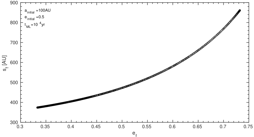
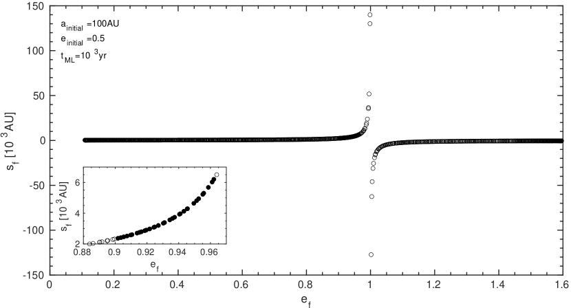
Figure 1: Example of the simulated data. Left plot: The simulated system is $m_{1i}=6.6M_{\odot}$, $m_{{\rm 1f}}=1.6M_{\odot}$ , $m_{2}=0.3M_{\odot}$, $a_{i}=100{\rm AU}$, $e_{i}=0.5$ and $T_{{\rm ML}}=10^{4}{\rm yr}$ with a linear mass loss function. The average final separation, $s_{f}$ is plotted against the final eccentricity for $1000$ equally spaced initial mean anomaly. The maximal $s_{f}$ is below $900{\rm AU}$ hence not satisfying condition (14). Right plot: the same systems as left plot only with $T_{{\rm ML}}=10^{3}{\rm yr}.$ In this case fraction of the initial values of the mean anomaly result in a binary breakup, $e_{f}>1$ and $s_{f}<0$. The zoomed in caption is the small fraction of the initial mean anomaly that satisfies the conditions (14).

Table 2: Example of the simulated function $F_{a_{i}}\left(e_{i},T_{{\rm ML}}\right)$ for $a_{i}=100{\rm AU}$ and for linear mass loss function and uniform initial eccentricity distribution. In this case only $T_{{\rm ML}}=10^{3}{\rm yr}$ satisfied the condition (14). For this set of initial conditions we did not simulate $e_{i}>0.5$ because for these systems the pericenter is too close to the inner binary orbit and the triple stability criteria breaks.

Example for the value of $F_{a_{i}}\left(e_{i},T_{{\rm ML}}\right)$ for $a_{i}=100{\rm AU}$
fractions	$e=0.1$	$e=0.2$	$e=0.3$	$e=0.4$	$e=0.5$
$T_{{\rm ML}}=10{\rm yr}$	$0$	$0$	$0$	$0$	$0$
$T_{{\rm ML}}=100{\rm yr}$	$0$	$0$	$0$	$0$	$0$
$T_{{\rm ML}}=1000{\rm yr}$	$0.308$	$0.09$	$0.056$	$0.042$	$0.033$
$T_{{\rm ML}}=10000{\rm yr}$	$0$	$0$	$0$	$0$	$0$

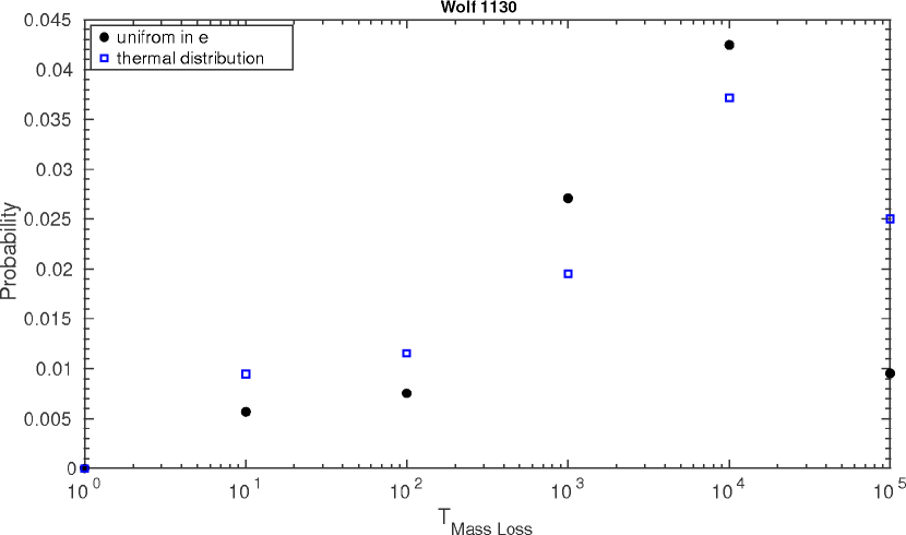
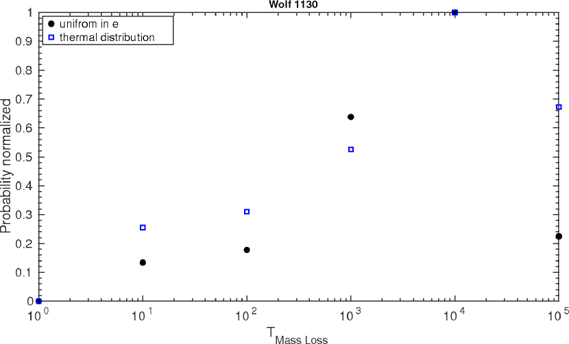
Figure 2: Upper plot: the probability of the mass loss timescale from the observed Wolf 1130 system for the linear mass loss case. The black circles (blue squares) correspond to uniform distribution (thermal distribution) of initial eccentricity. The most probable timescale is $T_{{\rm ML}}=10^{4}{\rm yr}$. Bottom plot: Is the normalized version of the upper plot to the maximal value for each distribution, in both cases is $T_{{\rm ML}}=10^{4}{\rm yr}$.

3.1.2 The case of an exponential mass-loss evolution

In this subsection we present the results for the exponential mass loss scenario, namely $M\left(t\right)_{{\rm binary}}=m_{1i}e^{-t\gamma}$ where $\gamma=-\ln\left(m_{1f}/m_{1i}\right)/t_{{\rm ML}}$. We follow the same procedure as described in subsection 3.1.1. Figure 3 presents the probability (upper) and the normalized probability to the maximal value (bottom). The same as the linear mass loss scenario the most probable mass loss timescale is $T_{{\rm ML}}=10^{4}{\rm yr}.$ For the uniform eccentricity distribution this timescale is more probable than $10^{3}{\rm yr},10^{2}{\rm yr},10{\rm yr}$ by a factor of $2.1,5.6,17.2$ respectively. Moreover, we find zero probability for $T_{{\rm ML}}=1{\rm yr}$ and $T_{{\rm ML}}=1{\rm 0^{5}yr}$. While for the thermal distribution case this timescale is more probable than $10^{5}{\rm yr,}10^{3}{\rm yr},10^{2}{\rm yr,10{\rm yr}}$ by a factor of approximately $60,2.1,2.8,6.3$ respectively. For the thermal eccentricity distribution we find zero probability for $T_{{\rm ML}}=1{\rm yr}.$

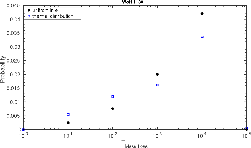
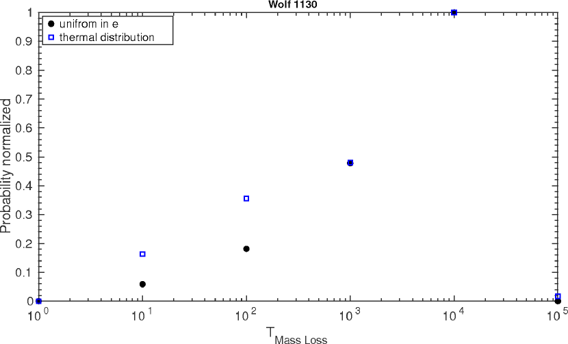
Figure 3: Same as Figure 2. Also for the exponential mass loss case the most probable mass loss timescale is $T_{{\rm ML}}=10^{4}{\rm yr}$ for the system Wolf 1130.

4 Case of GD 319

GD 319 is a triple system (Saffer et al., 1998; Farihi et al., 2005) at a distance of $\sim 436.5{\rm pc}.$ The inner binary consists of a subdwarf B star (sdB) of mass $\sim 0.5M_{\odot}$ with a close unseen companion (Saffer et al., 1998) of type dM. The tertiary is an M3.5 dwarf with mass $\sim 0.25M_{\odot}$ (Farihi et al., 2005) at a separation of $\sim 54914{\rm AU}$ from the inner binary with a common proper motion. The inner orbit has a $0.6$ day period.

As in the previous case binary_C code by was used to find a zero age main sequence binary that will evolve to form the observed GD 319. We find the following best fir parameters: for a Solar metallicity the primary begins with $m_{1}=1.5M_{\odot}$ and the secondary with $m_{2}=0.5M_{\odot}.$ The initial circular orbital separation is $a=350R_{\odot}$, as listed in Table 3. After $2.8{\rm Gyr}$ CEE commences. At the end of CE phase the sdB has a mass of $\sim 0.5M_{\odot}$ and the binary period is $P\approx 0.5$ day, consistent with the inferred parameters the observed GD 319 system.

Table 3: binary_C parameters used to evolve the simulated zero age main sequence binary into the observed GD 319AB.

binary_C parameters for GD 319AB
$m_{1}\left[M_{\odot}\right]$	$m_{2}\left[M_{\odot}\right]$	$a\left[R_{\odot}\right]$	$e$	$\alpha_{{\rm CE}}$	$\lambda_{{\rm CE}}$	$\lambda_{{\rm ion}}$
$1.5$	$0.5$	$350$	$0$	$0.2$	$-1$	$0$

4.1 Numerical calculation

We initiated the primary (the post-CE binary now treated as a point mass) with initial mass of $m_{1i}=2M_{\odot}$ and final mass following CEE of $m_{1f}=1M_{{\rm\odot}}.$ The secondary mass is $m_{2}=0.25M_{\odot}$. We repeat the same type of analysis as described for the Wolf 1130 system, using the same sampling of parameters and mass-loss functions. We only changes the separation and mass-loss timescale ranges to $a_{i}=50,100,300,500,1000,10000{\rm AU}$ and $t_{{\rm ML}}=1,10,10^{2},10^{3},10^{4},10^{5},10^{6}{\rm yr},$ respectively, corresponding to the wider separation of this system and the longer period of the outer orbit.

For this system we search for the following conditions (Dupuy & Liu, 2011). For a uniform distribution of the initial eccentricities

$$4.118\cdot 10^{4}{\rm AU}<s_{f}<11.1\cdot 10^{4}{\rm AU}$$

and for the thermal distribution we use

$$3.78\cdot 10^{4}{\rm AU}<s_{f}<11.3\cdot 10^{4}{\rm AU}.$$ (15)

The rest of the numerical treatment is identical to the one described at subsection 3.1.

4.1.1 The case of a linear mass-loss evolution

In this subsection we present the likelihood results of the mass loss timescales for the linear mass loss function. In Figure 4 (upper) we present the likelihood for each timescale, black circles and blue squares represent uniform distribution and thermal distribution of the initial eccentricity, respectively. The bottom panel of Figure 4 shows the relative likelihood, namely the ratio of the probabilities of all the calculated timescales to the most probable one.

We find that for the uniform eccentricity distribution the most probable timescale is $T_{{\rm ML}}=10^{3}$, which is as likely as the case of $T_{{\rm ML}}=10^{4}{\rm yr}$ and $T_{{\rm ML}}=10^{5}{\rm yr}$ . This timescale is more probable by a factor of approximately $17$, $21.7$ and 100 than the case of $10{\rm yr}$, $100{\rm yr}$ and $10^{6}$, respectively. Unlike the similar likelihood for the $10^{4}{\rm yr}$ and $10^{5}{\rm yr}$ timescales.

For the thermal distribution of the initial eccentricity we find similar results. The most probable mass loss timescale is $T_{{\rm ML}}=10^{4}$. This timescale is significantly more likely than the $10{\rm yr}$, $100{\rm yr}$ or $10^{6}$ yrs cases by factors of approximately $17,20,6.7$, respectively. While the mass loss timescale of $10^{3}{\rm yr}$ and $10^{5}{\rm yr}$ share the likelihood of a factor of $1.001$ and $1.04$ respectively. The probability of $T_{{\rm ML}}=1{\rm yr}$ is zero for both initial eccentricity distributions.

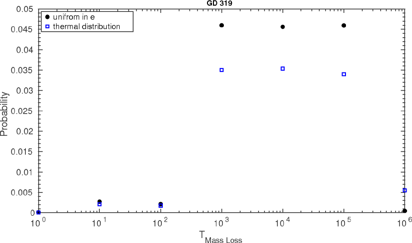
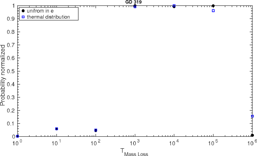
Figure 4: Upper plot: the probability of the mass loss timescale from the observed GD 319 system for the linear mass loss case. The black circles (blue squares) correspond to uniform distribution (thermal distribution) of initial eccentricity. The most probable timescale for the uniform initial eccentricity is $T_{{\rm ML}}=10^{3}{\rm yr}$ is $T_{{\rm ML}}=10^{4}{\rm yr}$ for while for the thermal eccentricity distribution is $T_{{\rm ML}}=10^{4}{\rm yr}$. Bottom plot: Is the normalized version of the upper plot to the maximal value for each distribution. It is clear that mass loss timescales of $10^{3}-10^{5}{\rm yr}$ are favorable compared to $1-10^{2}{\rm yr}$ and $10^{6}{\rm yr}.$

4.1.2 The case of an exponential mass-loss evolution

In this subsection we present the relative likelihood of mass-loss timescales for the exponential mass loss function for GD 319. We follow the same procedure as described in subsection 4.1.1. Figure 5 presents the probability (upper) and the normalized probability to the maximal value (bottom). We find that the most probable mass loss timescale for the uniform initial eccentricity distribution is $T_{{\rm ML}}=10^{5}{\rm yr}$. It is more probable by an approximate factor of $500,250,14.3$ for $1{\rm yr},10{\rm yr}$ and $100{\rm yr}$ mass loss timescales respectively. While it is approximately identical to the probability of $T_{{\rm ML}}=10^{4}{\rm yr}$, with a factor of $1.001.$ and similar probability to the mass loss timescales of $10^{3}{\rm yr}$ with only a factor of $1.04$ separates their likelihood. In our calculation $10^{6}{\rm yr}$ have zero probability.

For the thermal distribution of the initial eccentricity the most probable mass loss timescale is $T_{{\rm ML}}=10^{3}{\rm yr}$. It is more likely by approximate factors of $333.3,250$ and $21.7$ than the $1{\rm yr},10{\rm yr}$ and $100{\rm yr}$ mass-loss timescales cases, respectively. While it is similar for the mass loss timescales of $10^{4}{\rm yr}$ and $10^{5}{\rm yr}$. In this case the $10^{6}{\rm yr}$ timescale has zero probability.

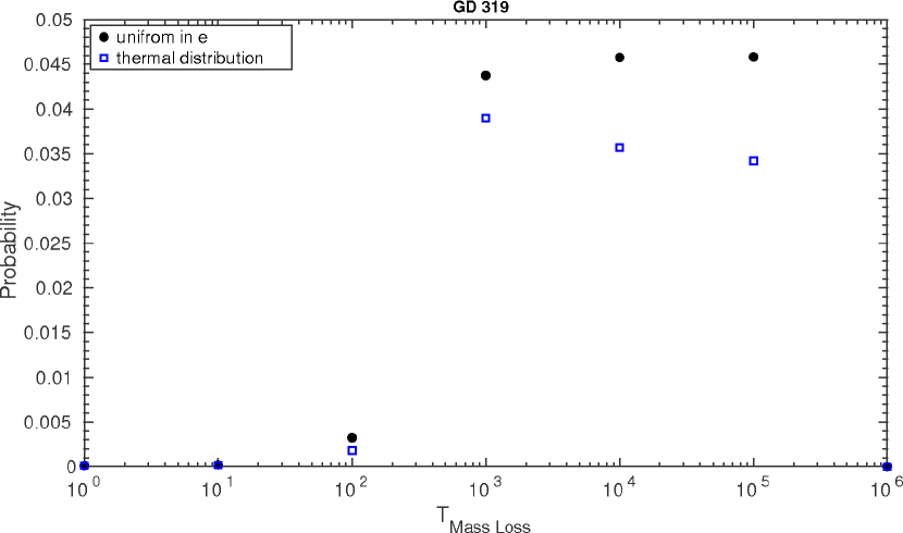
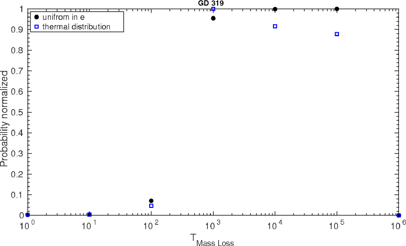
Figure 5: Upper plot: the probability of the mass loss timescale from the observed GD 319 system for the exponential mass loss case. The black circles (blue squares) correspond to uniform distribution (thermal distribution) of initial eccentricity. The most probable mass loss timescale for the uniform initial eccentricity is $T_{{\rm ML}}=10^{5}{\rm yr}$, but almost identical value to $T_{{\rm ML}}=10^{4}{\rm yr}$. For the thermal eccentricity distribution is $T_{{\rm ML}}=10^{3}{\rm yr}$. Bottom plot: Is the normalized version of the upper plot to the maximal value for each distribution. It is clear that mass loss timescales of $10^{3}-10^{5}{\rm yr}$ are favorable compared to $1-10^{2}{\rm yr}$ and $10^{6}{\rm yr}.$

5 Discussion

In order to calculate the results in sections 3 and 4 we made use of several assumptions, which we discuss below.

• We assumed that the third companion with similar proper motion is a bound companion. This is a commonly used assumption in the study of wide binaries. If the companion was originally bound but the triple was disrupted due to mass-loss, its separation would grown in time, and would far exceed the observed separation after only a few $10^{4}-10^{5}$ yrs, much longer than the cooling age of the observed WD which is $\sim 3.4{\rm Gyr}$ for Wolf 1130 (Mace et al., 2018).

• Mass loss timescale. We assumed the mass loss timescale from the inner binary during the CEE is equal to the mass loss timescale from the outer binary. This is not necessarily true when the mass ejected from the envelope have a wide velocity spread. Our ignorance on the ejection mechanism required us to make this simplifying assumption. Nevertheless, if we assume the mass ejected is ejected with velocities similar to escape velocities from a giant star, roughly $v\sim 30{\rm kms^{-1}}$ and the spread of the ejected velocity is $\sim 10\%$, namely $\Delta v\sim 3{\rm kms^{-1}}$ we get the crossing time for the total mass of the ejected envelope to cross the systems beyond the outer companion is

  $$\Delta T\approx a\times\frac{\Delta v}{v^{2}}=\left(\frac{a}{1000{\rm AU}}\right)\times 15.8{\rm yr,}$$ (16)

  and therefore we can not constrain CE-ejection timescales shorter than this range. However, the most likely timescales we find far exceed this short timescale, and therefore does not affect our conclusions.

• In this paper we consider two very different mass loss functions: linear in time (11) and exponential in time (12). We find that regardless of the chosen functional form of the mass-loss we find similar mass loss timescale constraints, suggesting the overall method is generally robust to the mass loss function.

• We only analyzed the data of two specific systems. Given the small statistics, in principal it is possible that in these two systems a third companion survived a shorter timescale mass-loss stage than the most probable one we find. Therefore although our results are suggestive of long timescales for CE-ejection, more systems should be analyzed in order to further support or refute these preliminary results.

• Throughout the paper we assumed the mass-loss is isotropic. An unisotropic mass-loss, possibly expected in CE-ejection (Taam & Ricker, 2010) might somewhat change the results, but is beyond the scope of this paper focusing on the presentation of the basic method and its initial testing.

In this paper we make use of a third wide-orbit companion to constrain the mass-loss timescale. We should note that a somewhat related idea was used by El-Badry & Rix (2018) to constrain natal kicks of WD, although they used a generalized statistical analysis, and not accounted for the detailed evolution of each system. We also note that they did not consider the treatment of prompt mass-loss which is relevant for their wider systems, and it is therefore possible that the cut-off they find in wide-separation is not related to WD kicks, but in fact corresponds to the range where the mass-loss timescale from AGB stars becomes comparable or shorter than the orbital period of the wide companions, as we discussed in this paper.

6 Summary

Common-envelope evolution plays an important role in the evolution of interacting binaries, but it is not well understood. Various different models were suggested to explain the envelope-ejection process, some of which differ in the the expected timescale involved in the ejection. Here we proposed a method to constrain the CE mass-loss timescales in CE-binaries, making use of CE-binaries with wide-orbit third companions. The orbits and survival of such third companions strongly depends on the timescale of the mass-loss and can therefore be used to con train them. We describe the orbital evolution due to mass-loss, and apply our method on two test cases of observed post-CE binaries which are part of wide triple systems, Wolf 1130 and GD 319. We find the most probable mass-loss timescales for these systems of $10^{3}-10^{5}{\rm yr}$ are longer than the timescales expected in most of the suggested models for CE-ejection, but they could be consistent with CE-ejection through dust-driven winds Glanz & Perets (2018). These results are currently based only on these two test-cases, and depend to some extent on the specific assumptions taken, and further analysis of additional systems is desired on order to provide further support, or refute them. Nevertheless, the general method suggested is robust, and can be used in the future on large samples.

Though based on two cases, the long CE-ejection timescales we infer do suggest significant challenge to most of the CE-models suggest to-date and are in tension with their expectations.

References

- Blaauw (1961) Blaauw A., 1961, Bull. Astron. Inst. Netherlands, 15, 265
- Clayton et al. (2017) Clayton M., Podsiadlowski P., Ivanova N., Justham S., 2017, MNRAS, 470, 1788
- De Marco et al. (2011) De Marco O., Passy J.-C., Moe M., Herwig F., Mac Low M.-M., Paxton B., 2011, MNRAS, 411, 2277
- Dupuy & Liu (2011) Dupuy T. J., Liu M. C., 2011, ApJ, 733, 122
- El-Badry & Rix (2018) El-Badry K., Rix H.-W., 2018, MNRAS, 480, 4884
- Farihi et al. (2005) Farihi J., Becklin E. E., Zuckerman B., 2005, ApJS, 161, 394
- Glanz & Perets (2018) Glanz H., Perets H. B., 2018, MNRAS, 478, L12
- Hills (1983) Hills J. G., 1983, ApJ, 267, 322
- Hut et al. (1995) Hut P., Makino J., McMillan S., 1995, ApJ, 443, L93
- Ivanova et al. (2013) Ivanova N., et al., 2013, A&ARv, 21, 59
- Ivanova et al. (2015) Ivanova N., Justham S., Podsiadlowski P., 2015, MNRAS, 447, 2181
- Izzard et al. (2004) Izzard R. G., Tout C. A., Karakas A. I., Pols O. R., 2004, MNRAS, 350, 407
- Izzard et al. (2006) Izzard R. G., Dray L. M., Karakas A. I., Lugaro M., Tout C. A., 2006, A&A, 460, 565
- Izzard et al. (2009) Izzard R. G., Glebbeek E., Stancliffe R. J., Pols O. R., 2009, A&A, 508, 1359
- Jeans (1961) Jeans J. H., 1961, Astronomy and cosmogony
- Mace et al. (2013) Mace G. N., et al., 2013, ApJ, 777, 36
- Mace et al. (2018) Mace G. N., et al., 2018, ApJ, 854, 145
- Moe & Di Stefano (2017) Moe M., Di Stefano R., 2017, ApJS, 230, 15
- Paczynski (1976) Paczynski B., 1976, in Eggleton P., Mitton S., Whelan J., eds, IAU Symposium Vol. 73, Structure and Evolution of Close Binary Systems. p. 75
- Passy et al. (2012) Passy J.-C., et al., 2012, ApJ, 744, 52
- Saffer et al. (1998) Saffer R. A., Livio M., Yungelson L. R., 1998, ApJ, 502, 394
- Taam & Ricker (2010) Taam R. E., Ricker P. M., 2010, New Astron. Rev., 54, 65
- Tokovinin & Kiyaeva (2016) Tokovinin A., Kiyaeva O., 2016, MNRAS, 456, 2070
- van den Heuvel (1976) van den Heuvel E. P. J., 1976, in Eggleton P., Mitton S., Whelan J., eds, IAU Symposium Vol. 73, Structure and Evolution of Close Binary Systems. p. 35