Using Deep Learning to Extend the Range of
Air Pollution Monitoring and Forecasting

Abstract

Across numerous applications, forecasting relies on numerical solvers for partial differential equations (PDEs). Although the use of deep-learning techniques has been proposed, actual applications have been restricted by the fact the training data are obtained using traditional PDE solvers. Thereby, the uses of deep-learning techniques were limited to domains, where the PDE solver was applicable.

We demonstrate a deep-learning framework for air-pollution monitoring and forecasting that provides the ability to train across different model domains, as well as a reduction in the run-time by two orders of magnitude. It presents a first-of-a-kind implementation that combines deep-learning and domain-decomposition techniques to allow model deployments extend beyond the domain(s) on which the it has been trained.

1 Introduction

Detrimental effects of air pollution on human health are long-studied. The WHO attributes 3.8 million deaths per annum to air pollution globally [1]. In many cities across the developed world, vehicle emissions are the dominant source of air pollutants [2], contributing around 70% of emissions of nitrogen oxides ($\mathrm{NO_{x}}$) [3], and up to 50% of particulate-matter pollution [4].

Quantification, evaluation, and mitigation of these effects require systems to estimate contribution of traffic volumes to air pollution. Traditionally, this is done by combining estimates (either observed or modelled) of traffic volumes, or rather the associated pollution-generation estimates, with weather observations in dispersion models that resolves a set of partial differential equations (PDE) to compute the desired pollution distributions. This approach is limited in three ways: the PDE model is computationally expensive, requires considerable domain expertise, and is cumbersome to parameterise for further geographical locations. The computational expense restricts the meshes that can be resolved, in terms of the spatial extent, spatial resolution, and ultimately, the number of discrete sources of pollution.

An alternative approach leverages the capabilities of deep learning (DL) to develop rapid solvers that can scale to any domain size. As an example of the state of the art in the area, James et al. [5] recently reported a factor of 5,000 computational speed-up compared to that of a leading PDE solver. Considering that the PDE solver is used to generate the outputs to train the DL model on, however, the model is still limited to the domain that the PDE solver can be run on. We integrate DL together with techniques from PDE-based domain decomposition to present an approach that learns the pollution dispersion at independent, neighbouring meshes and merges what has been learned into a single unified model for the region. More specifically, a PDE model for air pollution is used to generate sufficiently large volumes of data to facilitate the use of surrogate or reduced-order models [6] using deep artificial neural networks [7]. The model is deployed independently for a series of meshes with each representing a subset of a geographical domain and the DL model trained on the outputs of these meshes and merged in a recurrent neural networks (RNN) [8] type implementation to provide a single DL model of the entire region. The surrogate model serves as a computationally lightweight representation of the PDE-based model.

In our approach, the DL was trained on small domains and then applied to larger domains, with consistency constraints ensuring that the solutions are physically meaningful even at the boundaries of the domains. Our contributions are as follows:

• definition of the consistency constraints, wherein the output for one mesh is used to constrain the output for another mesh.

• methods for applying the consistency constraints within the training of a DL, which allows for an increase in the extent of the spatial domain by concatenating the outputs of several PDE-based models and considering conditions at neighbouring mesh interface.

• a numerical study of the approach on a pollution-forecasting problem, wherein we show the test mean absolute error (MAE) against PDE model and sensor data.

2 Related Work

A long-standing challenge in applied mathematics is the boundary-value problem, which consists in imposing boundary conditions at the defined internal or external boundaries of the region that is governed by a PDE. Such boundary conditions are additional constraints that usually come from field measurements, change of topology, or external models. Ensuring that the PDEs are solved, while embedding the boundary conditions, is the challenge of many practical engineering applications. Examples include resolution of the Saint-Venant [9] and Lighthill–Whitham–Richards (LWR) [10] equations, for water and transport network problems, respectively. In atmospheric pollution modelling, one considers the advection-diffusion equation [11, see equation 2.2] and the stochastic-coagulation equation [12], while financial modelling often considers Black-Scholes models and its numerous (stochastic) variations [13]. Throughout, there are different types of boundary problems depending on whether the function, derivative, or variable itself is known at the boundary. Among the numerical methods to solve this boundary-value problem for PDEs, prominent examples are the Godunov’s scheme [14], which involves solving a Riemann problem [15] at each defined cell interface, the Lax-Friedrichs method [16], which relies on the introduction of a viscosity term, and the Galerkin method [17]. The interested reader can refer to e.g. [15] for a discussion on the topic.

In practice, such discontinuities may be either inherent to the physics itself (proper boundary conditions, different models due to different flux functions, e.g., change from a motorway traffic network to a urban traffic network, different data sources for different regions in space) or artificial (software limitations, limited run-time, different entities providing different models). To our knowledge, our proposed approach is the first to address the discontinuities caused by the (arbitrary or not) discretisation in space of the grid where the forecasting is done via surrogate DL model(s) to the underlying PDE model(s).

In the problem presented in this paper, two classes of boundary conditions are considered: first, external boundary conditions that describe influx of pollutants to the domain (e.g., traffic volumes, wind conditions), and second, internal boundary conditions that can be enforced to ensure consistency between neighbouring domains. The latter can be considered a variant of the additive Schwarz method widely applied in the solution of partial differential equations. The additive Schwarz method provides an approximate solution for a boundary value problem by splitting it into boundary value problems on smaller domains and adding the results [18]. These domain-decomposition techniques are widely studied in parallel-computing applications and consist of solving subproblems on various subdomains while enforcing suitable consistency constraints between adjacent subdomains, until the local problems converge to an approximation of the true solution [19]. It proceeds by splitting the global domain into a set of smaller overlapping or non-overlapping subdomains. In each step, an iterative method resolves the partial differential equations restricted to individual subdomains and then coordinates the solution between adjacent subdomains. In our study, we consider an approach that trains a DL model on a set of subdomains with an iterative reduction used to enforce a physically meaningful relationship between adjacent subdomains. A large number of domain-decomposition approaches exist and we refer to the books by Quarteroni and Valli [20] and Smith et al. [21] for an extensive introduction.

Our methods draw on domain-decomposition implementations and recent work within applying DL to PDE-based models. A large body of literature exist on the use of neural networks with PDE-based models [22, 23, 24, 25, 26, 27, 28, 29], across a variety of applications such as fluid modelling [30], combustion modelling [31], and the geosciences [32, 33]. More recently, the use of DL as surrogate for expensive physics-based models has been investigated [34, 5, 35, 36, 31, 37]. In these latter studies, a solver for PDEs has been used to obtain hundreds of thousands of outputs corresponding to hundreds of thousands of inputs. The DL has then been used as means of non-linear regression between the inputs and outputs. In particular, Tompson et al. [34] considered a convolutional neural network (CNN), while Wiewel et al. [35] considered long short-term memory (LSTM) units within a recurrent neural network (RNN). In a more abstract setting, Sirignano and Spiliopoulos [38] have explored the use of mesh-free DL in what they call deep Galerkin methods. Throughout, the applications of DL have been limited in scale to the domains that had been tractable for the traditional solver for PDEs.

A wide-variety of recent applications of deep-learning in numerical analysis include non-intrusive reduced basis [36] and related [31, 37] methods for the construction of reduced-order models, learning PDEs from data [39, 40], and the detection of troubled cells in two-dimensional unstructured grids [41, 42].

A further stream of related work has been started by Chen et al. [43], who presented a novel approach to approximate the discrete series of layers between the input and output state by acting on the derivative of the hidden units. At each stage, the output of the network is computed using a black-box differential equation solver which evaluates the hidden unit dynamics to determine the solution with the desired accuracy. In effect, the parameters of the hidden unit dynamics are defined as a continuous function, which may provide greater memory efficiency and balancing of model cost against problem complexity. The approach aims to achieve comparable performance to existing state-of-the-art with far fewer parameters, and suggests potential advantages for time series modelling. For follow-up work in this stream, see [44, 45]. On a similar note Han et al. [46] investigated approaches to solve PDEs using deep learning gradient-based approaches. By reformulating the PDEs as backward stochastic differential equations the unknown is solved for using a gradient-descent approach based on reinforcement learning.

Finally, there is a long history of the use of machine learning in pollution monitoring [47, 48, 49, 50, e.g.]. Recently, Zhu et al. [50] considered a coarse (0.25 degree resolution) grid of mainland China, with more than two years of air quality measurement and meteorological data, without any further insights, such as pollution sources, surface roughness, the reaction model, the multi-resolution aspects, or similar. Qi et al. [49], considered a joint model for feature extraction, interpolation, and prediction while employing the information pertaining to the unlabelled spatio-temporal data to improve the performance of the predictions. These approaches use the measurement data without regard to the physics, which limits their performance, given the sparsity and costs of presently available sensors.

3 Our Approach

We present the first attempt to apply a domain decomposition to training of a surrogate model of a partial differential equation (PDE). At a high level, our approach consists of training a deep-learning model for each subdomain, while providing a method to ensure consistency across neighbouring domains. By enabling communication between subdomains via constraints, predictions for one subdomain can benefit from information outside of the subdomain. This makes it possible to scale to the whole domain such that the accuracy of the predictions and its ability to generalise is increased, compared to models trained on the individual subdomains without the consistency constraints.

Let us consider an index-set $\mathcal{M}$ of meshes $M_{m}$, $m\in\mathcal{M}$, with sets of $n_{m}$ mesh points $P(M_{m})$. The output of each PDE-based simulation on such a mesh consists of values in $\mathbb{R}^{d_{m}}$ at each point of $P(M_{m})$. Often, a small sub-set of $n_{m}^{(r)}$ of such points is of particular interest, which we call receptors $R(M_{m})$; the remainder of the points represents hidden points $H(M_{m})$. The receptors and hidden points thus partition the mesh points $P(M_{m})=H(M_{m})\cup R(M_{m})$, with $n_{m}=n^{(h)}_{m}+n^{(r)}_{m}$. Further, let us consider the index-set $\mathcal{B}\subseteq\mathcal{M}\times\mathcal{M}$ of boundaries $B_{mn}$ of meshes. Such a possibly infinite boundary $B_{mn}\subseteq P(M_{m})\times P(M_{n})$ links pairs of points from the two meshes. To each boundary $B_{mn}$ we associate a constant $\epsilon_{mn}$ that reflects the importance of this boundary. Further, for each mesh $M_{m}$ we have an ordered set of simulations indexed with time $t\in\mathbb{Z}$, where each simulation is defined by the inputs $x^{(m)}_{t}\in X^{(m)}_{t}$ and a set of outputs $y^{(m)}_{t}\in(\mathbb{R}^{d_{m}})^{\times n_{m}}$. Often, one wishes to consider $y^{(m)}_{t}$ being part of $x^{(m)}_{t+k}$ for some $k>0$, in a recurrent fashion.

Our aim is to minimise residuals subject to consistency constraints, and thus exchange information between neighbouring domains and ensure physical “sanity” of the results, i.e.,

$$r^{*}= \min_{f}\sum_{t}\sum_{m\in\mathcal{M}}\left\|\operatorname{proj}_{R(M_{m})}\!\left(y^{(m)}_{t}-f^{(m)}\!\big{(}x^{(m)}_{t}\big{)}\right)\right\|$$ (1)

$$\operatorname{s.t.}\;\forall t\;\forall(m,n)\in\mathcal{B}\;\forall(p_{1},p_{2})\in B_{mn}:$$

$$\operatorname{prox}\!\left(\operatorname{proj}_{\{p_{1}\}}\!f^{(m)}\big{(}x^{(m)}_{t}\big{)}\,,\;\operatorname{proj}_{\{p_{2}\}}\!f^{(n)}\big{(}x^{(n)}_{t}\big{)}\right)\leq\epsilon_{mn}\,,$$

where $\operatorname{proj}_{Q}:(\mathbb{R}^{d_{m}})^{\times n_{m}}\to(\mathbb{R}^{d_{m}})^{\times|Q|}$ is a projection operator that projects the array of outputs at all points onto the outputs at a subset of points $Q\subset P(M_{m})$, $\operatorname{prox}$ is a proximity operator, the decision variable defines the mapping $f=\{f^{(m)}\}^{m\in\mathcal{M}}$, whereby $f^{(m)}\!\big{(}x^{(m)}_{t}\big{)}$ represents the output of a non-linear mapping between inputs and PDE-based simulation outputs at the points of the mesh, $f^{(m)}:X^{(m)}_{t}\to(\mathbb{R}^{d_{m}})^{\times n_{m}}$, on each independent mesh $M_{m}$, which can be seen as a non-linear regression, and $\epsilon_{mn}$ is a constant specific to $(m,n)\in\mathcal{B}$. Thinking about a system based on a PDE, the projection operator onto $R(M_{m})$ can be thought of as selecting the receptors, which are positions at which the solution to the PDE is evaluated. In principle, the set of mesh points can also contain points for which no estimates from the ground-truth model are generated.

Notice that $f^{(m)}:X^{(m)}_{t}\to(\mathbb{R}^{d_{m}})^{\times n_{m}}$ should be seen as a non-linear regression; we provide examples of $f^{(m)}$ in the following sections. The requirement of physical “sanity” is usually a statement about smoothness of the values of the mapping $f^{(m)}$ across the boundaries of two different meshes and represents the fact that processes in one mesh impact direct neighbours. To be able to compare those values, we require that the dimensions are the same, that is $\forall m,n\in\mathcal{M}:\;d_{m}=d_{n}\equiv d$. For example, for $\operatorname{prox}$ being the norm of a difference of the arguments, “smooth” at a point at the boundary of two meshes means that the values predicted within the two meshes at that point are numerically close to each other. Also adding the norm of the difference of their gradients to that makes it a statement about the closeness of their first derivatives too. Technically, “smoothness” is a statement about all their higher derivatives as well, however, we will only concern ourselves with their values, or zeroth order of derivatives, for now. Notice though that generically this is an infinitely large problem.

The constrained optimisation problem equation 1 can be solved by Lagrangian relaxation techniques [51], wherein for Lagrange multipliers $\lambda:=\{\lambda^{(m)}_{t}\}^{m\in\mathcal{M}}_{t\in\mathbb{Z}}$ we have an unconstrained optimisation problem, as suggested in equation 2 in Figure 1

$$r^{*}= \inf_{f,\,\lambda}\sum_{t}\Bigg{(}\sum_{m\in\mathcal{M}}\left\|\operatorname{proj}_{R(M_{m})}\!\left(y^{(m)}_{t}-f^{(m)}(x^{(m)}_{t})\right)\right\|$$ (2)

$$+\sum_{(m,n)\in\mathcal{B}}\sum_{(p_{1},p_{2})\in B_{mn}}\lambda^{(m)}_{t}\operatorname{prox}\!\left(\operatorname{proj}_{\{p_{1}\}}\!f^{(m)}\big{(}x^{(m)}_{t}\big{)}\,,\operatorname{proj}_{\{p_{2}\}}\!f^{(n)}\big{(}x^{(n)}_{t}\big{)}\right)\Bigg{)}\,$$

Figure 1: The Lagrangian relaxation.

Under mild conditions [52, Proposition 3.1.1], there exist $\lambda_{t}^{(m)}$, $t\in\mathbb{Z}$, such that the infimum over $f^{(m)}$ coincides with $r^{*}$, for each $m\in\mathcal{M}$. Clearly, if at least some of the boundaries $B_{mn}$ are infinite, then the optimisation problem is infinite-dimensional.

Next, one can borrow techniques from iterative solution schemes in the numerical analysis domain. Notice that the first term in equation 2 is finite-dimensional and separable across the meshes. For each mesh $M_{m}$, $m\in\mathcal{M}$, the above can be computed independently. Further, one can sub-sample the boundaries to obtain a consistent estimator. Subsequently, one could solve the finite-dimensional projections of equation 2, wherein each new solution will increase the dimension of $\lambda^{(m)}_{t}$. While this is feasible in theory, the inclusion of non-separable terms with $\lambda^{(m)}_{t}$ would still render the solver less than practical.

Instead, we propose an iterative scheme, which is restricted to separable approximations. Let us imagine that during iteration $k$ and at time $t$, for a pair of points $(p_{1},p_{2})\in B_{mn}$ on the boundary indexed with $(m,n)\in\mathcal{B}$, we obtain values from the trained model at those points in the respective mesh, $\mathbb{R}^{d}\ni f^{(m)}_{p_{1},t}=\operatorname{proj}_{\{p_{1}\}}f^{(m)}\big{(}x^{(m)}_{t}\big{)}$ and $\mathbb{R}^{d}\ni f^{(n)}_{p_{2},t}=\operatorname{proj}_{\{p_{2}\}}f^{(n)}\big{(}x^{(n)}_{t}\big{)}$. While the two points $p_{1},p_{2}$ lie in two different meshes, we would like the model outputs at those points to eventually coincide for high enough $k$. For that, we iteratively construct vectors $\underline{\chi}_{p_{1},p_{2}}^{(k+1)}$ and $\overline{\chi}_{p_{1},p_{2}}^{(k+1)}\in\mathbb{R}^{d}$, which serve as lower and upper bounds on the values obtained from the training of $f^{(m)}$ at the $k^{\rm th}$ iteration. Those vectors can be updated through a variety of methods. A naïve example includes extracting some bounds based on the upper and lower limits of neighbouring meshes boundary values. In order to obtain convergence properties in a non-convex setting, we use an asymptotically vanishing shift term to adjust the interval according to the newly trained data, and a gradient term, according to

$${\underline{\chi}_{p_{1},p_{2}}^{(k+1)}}_{i}={\underline{\chi}_{p_{1},p_{2}}^{(k)}}_{i} +\frac{\kappa}{\sqrt{k}+\zeta}\left({\rm min}\!\left({f^{(m)}_{p_{1},t}}_{i},\,{f^{(n)}_{p_{2},t}}_{i}\right)-{\underline{\chi}_{p_{1},p_{2}}^{(k)}}_{i}\right)$$

$$+\frac{\kappa\sqrt{k}}{\sqrt{k}+\zeta}\left({\underline{\chi}_{p_{1},p_{2}}^{(k)}}_{i}-{\underline{\chi}_{p_{1},p_{2}}^{(k-1)}}_{i}\right)\,,$$

$${\overline{\chi}_{p_{1},p_{2}}^{(k+1)}}_{i}={\overline{\chi}_{p_{1},p_{2}}^{(k)}}_{i} +\frac{\kappa}{\sqrt{k}+\zeta}\left({\rm max}\!\left({f^{(m)}_{p_{1},t}}_{i},\,{f^{(n)}_{p_{2},t}}_{i}\right)-{\overline{\chi}_{p_{1},p_{2}}^{(k)}}_{i}\right)$$

$$+\frac{\kappa\sqrt{k}}{\sqrt{k}+\zeta}\left({\overline{\chi}_{p_{1},p_{2}}^{(k)}}_{i}-{\overline{\chi}_{p_{1},p_{2}}^{(k-1)}}_{i}\right)\,.$$ (3)

The free parameters $\kappa$ and $\zeta$ are tunable and resemble learning rates. In principle, they could be chosen dynamically, specific to each boundary $(m,n)$. Choosing them to be constants based on a greedy search across a limited parameter space eases the computational efforts.

For the first iterations, the boundary values are initialised using the minimum and maximum of the labels, respectively. Subsequently, we can form univariate (box, interval) constraints, restricting the corresponding elements of both $f^{(m)}$ at $p_{1}$ and $f^{(n)}$ at $p_{2}$ of the next iteration to the interval $\big{(}{\underline{\chi}_{p_{1},p_{2}}}_{i},{\overline{\chi}_{p_{1},p_{2}}}_{i}\big{)}$. Notice that replacing $\lambda^{(m)}_{t}$ with a constant $\lambda$ provides an upper bound on $r^{*}$, which is much easier to solve, computationally.

In the scheme, we consider a finite-dimensional projection of equation 2. For each $(m,n)\in\mathcal{B}$ we consider a finite sample $\hat{B}_{mn}\subset B_{mn}$ of pairs of points, for which we obtain

$$r^{*} =\min_{f,\lambda}\sum_{t}\Bigg{(}\sum_{m\in\mathcal{M}}\left\|\operatorname{proj}_{R(M_{m})}\left(y^{(m)}_{t}-f^{(m)}\big{(}x^{(m)}_{t}\big{)}\right)\right\|$$ (4)

$$\quad+\sum_{\begin{subarray}{c}(m,n)\in\mathcal{B}\\ (p_{1},p_{2})\in\hat{B}_{mn}\end{subarray}}\sum_{\begin{subarray}{c}l\in(m,p_{1})\\ p\in(n,p_{2})\end{subarray}}$$

$$\epsilon_{mn}\lambda\left\|\max\!\big{(}0,\underline{\chi}_{p_{1},p_{2}}-f^{(l)}_{p,t}\big{)}+\max\!\big{(}0,f^{(l)}_{p,t}-\overline{\chi}_{p_{1},p_{2}}\big{)}\right\|_{1}\!\Bigg{)}\,,$$

where we consider the function $\max:\mathbb{R}\times\mathbb{R}^{d}\to\mathbb{R}^{d}$ to operate element-wise. Further, when we consider $\lambda$ as a hyper-parameter, we obtain an optimisation problem separable in $m\in\mathcal{M}$, which in the limit of $|\hat{B}_{mn}|\to|B_{mn}|$ provides an over-approximation for any $\lambda$.

In deep learning, this scheme should be seen as a recurrent neural network (RNN). A fundamental extension of RNN compared to traditional neural network approaches is parameter sharing across different parts of the model. We refer to Goodfellow et al. [7] for an excellent overview and Figure 2 for a schematic illustration. Each training iteration provides constants $(\underline{\chi}_{p_{1},p_{2}},\overline{\chi}_{p_{1},p_{2}})$, which are used in the consistency constraints of the subsequent iteration. In terms of training the RNN, it is important to notice that equation 4 allows for very fast convergence rate even in many classes of non-linear maps $f$. For instance, when $f^{(m)}:X^{(m)}_{t}\to(\mathbb{R}^{d_{m}})^{\times n_{m}}$ is a polynomial of a fixed degree [53], then equation 4 is strongly convex, despite the max function making it non-smooth. The subgradient of the max function is well understood [54] and readily implemented in major deep-learning frameworks.

Figure 2: A schematic illustration of our recurrent neural network, where the recursion considers the consistency constraints defined by $\underline{\chi},\overline{\chi}$. In experiments described in Section 4, we use $q=50$ and $s=7$.

In numerical analysis, in general, and with respect to the multi-fidelity methods [55], in particular, our approach could be seen as iterative model-order reduction. The original PDEs could be seen as the full-order model (FOM) to reduce, and equation 1 could be seen as a high-fidelity data-fit reduced-order model (ROM), albeit not a very practical one, whereas equation 4 could then be seen as a low-fidelity data-fit ROM, which allows for rapid prediction.

In approximation theory, and learning theory that grew out of it, it is known since the work of [56] that even a feed-forward network with three or more layers of a sufficient number of neurons with, e.g., sigmoidal activation function allows for a universal approximation of functions on a bounded interval. It is not guaranteed, however, that the approximation has any further desirable properties, such as energy conservation etc. Our consistency constraints can be used to enforce such properties.

Fundamentally, the approach can be summarised as learning the non-linear mapping between inputs and predictions on each independent mesh, and iterating to ensure consistency of the solution across meshes. Such an approach draws on a long history of work on setting boundary conditions as consistency constraints in the solution of PDEs [57].

4 Methods

To illustrate this framework, we trained the DL for city-scale pollution monitoring, utilising:

• Pollution measurements and traffic data.

• Weather data (i.e., velocities, pressures, humidity, and temperatures in 3D).

• A given discretisation of a city in multiple meshes, corresponding to multiple geographic areas with their specificities.

Our test case was based in the city of Dublin, Ireland, for which real-time streams of traffic and pollution data (from Dublin City Council), and weather data (from the Weather Company) were available to us, but which did not have any large-scale models of air pollution deployed.

4.1 Air Pollution Forecasting

Our goal is to estimate the traffic-induced air pollution, specifically levels of NO₂ (which is closely related to $\mathrm{NO}_{\text{x}}$ overall) and $\mathrm{PM}_{10}$, for defined receptors across the city. We selected these pollutants and as they are central to major public health concerns particularly in relation to an observed increase of lung and heart diseases in cities across the developed world, and as they are mostly generated by vehicle emissions. In addition ozone $\mathrm{O}_{3}$ is typically produced as a result of complex reactions involving organic compounds as well as nitrogen oxides $\mathrm{NO}_{\text{x}}$.

Our prediction framework consisted of inputs of traffic volumes for a number of roadway links across the city, weather data, and an air-pollution dispersion model. Outputs consisted of periodic estimates of pollution levels. The typical approach in the traffic-induced air-pollution forecasting literature is to treat links as line sources. Dispersion models are, in fact, line-source models that describe the temporal and spatial evolution of vehicle emissions near roadways [58]. Gaussian-plume models consider a closed-form solution to the advection-diffusion equation under a series of simplifying and steady-state assumptions, see from equation 2.2 in [11]. The Caline [59], Hiway [60], and Aermod [61] suite of models are three examples of Gaussian plume EPA-developed models, while the latest releases of Caline (Caline 3 and 4) have had the widest adoption over the last decades, see e.g. Samaranayake et al. [62], and Aermod is the most recently developed, but licensed model. There also exist more sophisticated numerical models in the literature. One can name the non-steady-state Lagrangian puff modelling system, calPuff [63] or even CFD models such as the commercial Ansys Fluent model [64] relying on the discretization of air flow variables as finite control volumes. Finally, the machine learning family of air dispersion models should be mentioned, e.g. from multivariate analysis [65] to neural-network models [66].

In this work, we choose to use a Gaussian-plume model in its popular Caline-4 implementation, due to its wide use across the years. We are aware of the complexity of some of the air dispersion models of use in the literature. However, we selected the Gaussian plume model and its Caline 4 implementation for the sake of simplicity and reproducibility. Dealing with more complex models within our presented framework is not an impossible task, but would be an engineering challenge requiring the handling of possibly more air quality variables and possibly deeper DL models. This falls beyond the scope of this paper which aims at providing a proof of concept of our newly presented methodology.

In the adopted model, each pollutant is defined by its mass $C(\vec{x},t)$ at a location $\vec{x}=(x,y,z)$ and time $t$. See Figure 3 for an illustration of the propagation of a pollutant, assuming a wind direction along the $x$ axis. The pollutant is emitted from the source at height $h$, and the concentration profiles are given in the downwind directions, using the dispersion factors $\sigma_{z}$ and $\sigma_{y}$.

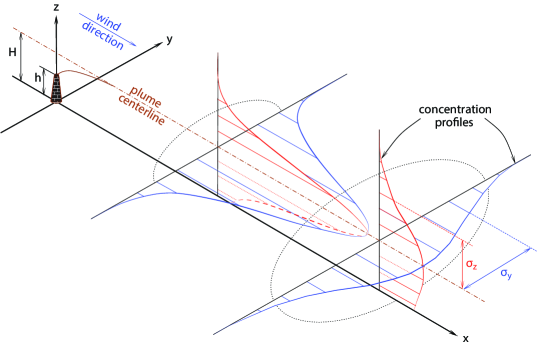
Figure 3: An illustration of the Gaussian Plume model, adapted from J. M. Stockie [11].

Following [11], the law of conservation of mass is

$$\frac{\partial C}{\partial t}+\nabla\cdot\vec{J}=S\,,$$ (5)

where $S(\vec{x},t)$ is a source or sink term, and $J(\vec{x},t)$ is the mass flux considering the effects of diffusion and advection. The equation reduces to

$$\frac{\partial C}{\partial t}+\nabla\cdot\left(C\vec{u}\right)=\nabla\cdot\left(\bf{K}\cdot\nabla C\right)+S\,,$$ (6)

where $\vec{u}$ is the wind velocity and $\bf{K}$ is the $3\times 3$ diagonal matrix of the space-diffusion coefficients, which are assumed to be functions of the downwind distance only, and thus all equal to $K(x)$. After proceeding with the change of variable

$$r=\frac{1}{u}\int_{0}^{x}K(\xi)d\xi\,,\quad$$ (7)

and assuming we either know the closed form of $K(x)$ from experimentally measured values or $K(x)$ is constant, the Gaussian Plume solution $c(r,y,z)$ of the advection-diffusion equation can then be derived, which for a homogeneous, steady-state flow and a steady-state line source of finite length $L$ is given by:

$$\frac{Q_{L}}{2u\sqrt{\pi r}}\exp\!\left(-\frac{z^{2}}{4r}\right)\left[f\left(\frac{y+L/2}{2\sqrt{r}}\right)-f\left(\frac{y-L/2}{2\sqrt{r}}\right)\right],$$ (8)

where $Q_{L}$ is a emission constant rate, and where $f(x)=2/\sqrt{\pi}\int_{0}^{x}\exp(-\xi^{2})d\xi$ is the error function. Note that, for low wind speeds, e.g. lower than $0.5~{}$\mathrm{m}\,\mathrm{s}^{-1}$$, the diffusion term cannot be neglected in the $x$-direction relative to the advection term, rendering equation 8 inaccurate. The interested reader may refer to [11], page 359-360, for more details.

4.2 The Implementation

We used Caline [59], the standard free dispersion-modelling suite, to solve the Gaussian Plume model for the inputs and outputs presented in the previous Section. We note while Caline is one of the “Preferred and Recommended Air Quality Dispersion Model” of the Environmental Protection Agency in the USA [67], it has significant practical limitations. Specifically, it is limited to 20 line sources (of traffic) and 20 receptors (prediction points) per computational run, which in turn forces an arbitrary in-homogeneous discretisation of the road network and is a strong motivation for the use of our cross-domain deep learning framework.

We implemented the approach for the use case of Dublin, Ireland. The area was partitioned into 12 domains, with 7-20 line sources of pollution in each subdomain. Inputs to the PDE solver comprised of hourly traffic volume data at each line source obtained (by aggregation of readings of traffic detectors) from the traffic control system (SCATS) used in Dublin, and hourly weather data (wind speed, direction, temperature, humidity) obtained from The Weather Company. Available training data comprised almost one year worth of hourly data from July 1^st 2017 to May 2^nd 2018. The outputs focused on concentrations of NO₂, and $\mathrm{PM}_{10}$ concentrations at predefined receptor locations, as illustrated in Figure 4. To circumvent the limitation on number of receptors allowed by Caline (20 receptors per computational run), we ran the Caline model 15 times with receptors positioned in different locations to give adequate spatial coverage of pollution estimates across the domain. Outputs were produced at 300 receptor locations within each subdomain giving a total of 3,600 estimates of pollution across the domain each hour for the 305-day study period. Caline-model specific parameters were chosen for each subdomain $M_{m}$ based on the state-of-the-art practices [58]: the emission factors based on the UK National Atmospheric Emissions Inventory database, dispersion coefficients based on the Caline recommendations (values for inner city, outer city areas), and background pollution levels chosen as the average time series values across the pollution measurements stations. This is in line with the usage of the Environmental Protection Agency of Ireland [68]. The background pollution levels were subtracted again from the Caline output to obtain an effective traffic contribution to the pollution concentrations. Each subdomain was then computed independently based on the specific traffic, weather, and model parameters for the locality.

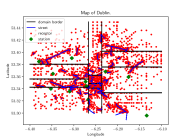
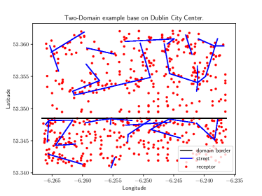
Figure 4: Left: Map of Dublin, partitioned into 12 domains (black lines), displaying the positions of line sources (blue lines), receptors (red dots), and measurement stations (green diamonds). Right: A close-up of Dublin city center, featuring two partitions with adjusted line sources close to the boundary (central partitions on the left).

The RNN model was implemented in Tensorflow [69] to obtain, in effect, the non-linear regression between the inputs and outputs, with the consistency constraints applied iteratively. That is, with each map from the inputs to the outputs, we obtained further consistency constraints to use in subsequent runs on the same domain. Features to the neural network consisted of the time step, the traffic line sources, the weather data, and a receptor location at each time step. Training label data consisted of the Caline outputs (without background pollution) for those features at the given receptor. From those features, we created design matrices, each row consisting of the spatial coordinates of the start and end points of the traffic line sources (up to 40 coordinate tuples per subdomain) and traffic volume measurements for each of the line sources, the weather data (wind speed, direction, directional standard deviation, temperature) for the locality, the coordinates of a receptor for which the pollution concentrations should be estimated (there are 300 locations per subdomain), and the hourly timestamp measured in seconds since January 1^st 1970. The training data inherently has the structure of a time series, and as such it would be sensible to combine all receptor locations of a given subdomain in the input of that time slice, if our problem would be a temporal forecasting one. However, our problem of combining several subdomains by imposing consistency constraints across the boundaries is primarily a geospatial one. For the consistency constraints, the models need to predict pollution concentrations at the subdomain boundaries, where no training data exists. That is: they need to learn the spatial relations of the underlying physics. As such, it is much more sensible to structure the learning set into spatial slices, predicting concentrations for one receptor at a time.

The timestamp input as well as the output labels were normalised between zero and one, whereas all other inputs were Gaussian normalised over each unit domain. Overall, the feature design matrix, $\mathbf{X}$, had 1,494,900 rows (number of hourly estimates of all 300 receptors over the near-yearlong period) and up to 107 columns (number of features for each subdomain estimate). For subdomains with fewer line sources, $\mathbf{X}$ had correspondingly fewer columns. The label design matrix, $\mathbf{Y}$, for model training was composed of the 1,494,900 Caline model runs, each of which comprises one Caline estimate of pollution for each receptor location within each subdomain. This process was repeated for each of the 12 subdomains and for each of the two pollutants considered (NO₂ and $\mathrm{PM}_{10}$), resulting in a total of 24 corresponding $\mathbf{X}$ and $\mathbf{Y}$ matrices provided as an input to the RNN model.

The cost function used the standard regularisation with the $\ell_{2}$-loss of the weights. For the consistency constraints, we choose $\zeta=1,\epsilon_{mn}=1$, and considered different values for $\lambda$ and $\kappa$. The final topology consisted of a multilayer perceptron (MLP) with seven layers, each having 50 nodes, with a leaky ReLU activation function with $\alpha=0.1$ after each layer [7]. Network training adopted the Adam optimisation algorithm with stochastic gradient descent on batches of size 128. The $\mathbf{X}$ and $\mathbf{Y}$ data were always randomly shuffled into two groups to form the training-data set composed of 90% of the 1,494,900 rows of data with the test-data set the remaining 10%. We trained for 25 epoch per iteration, with the consistency constraints between subdomains updated each iteration for a total of 20 iterations.

The complete source code has been released publicly under Apache license at https://github.com/IBM/pde-deep-learning, whereby further details of the implementation can be studied in detail. Likewise, all our data are freely available. Traffic-detector data used in the research are freely available from Dublin City Council. Weather data have been obtained from The Weather Company, an IBM business, under a licence. While we do not have rights to redistribute The Weather Company data, a free API key can be obtained to download the data from the vendor. Suggestions as to the model parameters are freely available from the Environmental Protection Agency, Ireland. The Caline package used for comparison is freely available from the California Department of Transportation (Caltrans). Pollution measurement data used in the comparison are freely available from Dublin City Council and Environmental Protection Agency, Ireland. We hope that this release of code and data stimulates further research in the field.

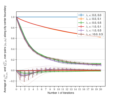
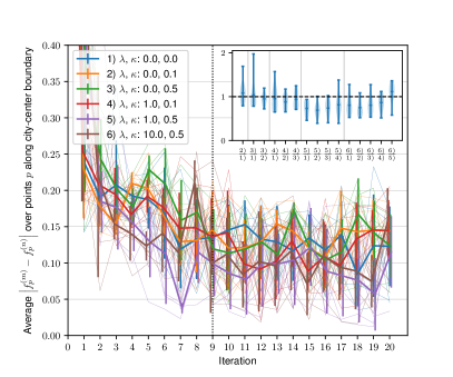
Figure 5: Effects of consistency constraints illustrated on two city-centre subdomains presented on the right in Figure 4. The individual experiments are shown as thin lines. Their average is shown as a thick line with error bars at one standard deviation. Left: Mean lower ($\underline{\chi}$) and upper ($\overline{\chi}$) values of the consistency constraint interval plotted across the iterations, i.e., two lines per colour. Right: Mean difference between output of the DL models along the boundary between the two subdomains illustrating how specification of appropriate consistency constraints reduces the difference between predictions at adjacent boundaries. The inset shows the ratios between this value for the different parameter specifications. The ratio is computed over all iterations greater or equal than nine (dashed lined) to allow training error to stabilise.

5 Results

First, to illustrate the workings of our approach, let us plot the convergence behaviour of the interval $(\underline{\chi},\overline{\chi})$ of equation 3 for the consistency constraints at the city-centre boundary for a few parameter combinations, as well as the convergence behaviour of the difference between the predicted values from the two neighbouring models along this boundary. In order to have clear boundary effects, we adjusted the street layout by bringing the streets in the southern subdomain closer to the boundary and pushing the streets in the northern subdomain further away, as illustrated on the right of Figure 4. In particular, Figure 5 (left) presents the evolution of the interval $(\underline{\chi}_{p_{1},p_{2}}^{(k)},\overline{\chi}_{p_{1},p_{2}}^{(k)})$ over iterations $k$, when averaged over the pairs $(p_{1},p_{2})$ of corresponding points on the boundary of the two subdomains. Clearly, we observe that $\underline{\chi}$ converges to $\overline{\chi}$, with rapid convergence especially in the first four iterations. Further, one may add that faster convergence with increasing $\kappa$ is observable up to a certain point. For higher values of $\kappa$, e.g., $\kappa=0.7$, one enters an oscillatory regime (not shown), which should be avoided. This behaviour can be understood by drawing an analogy between equation 3 and accelerated first-order optimisation methods: one can think of $\kappa$ as a learning rate. One should like to point out two caveats, though. First, this behaviour is stochastic: Notice the difference between the individual sample paths, which is due to the non-convexity of the problem and the variable performance of randomised algorithms therein. Second, this behaviour also does not translate to the values in $x^{(m)},x^{(n)}$ being the same, except for $\lambda$ sufficiently large and rather impractical. With these caveats, the behaviour demonstrates an iterative relaxation of the solution at neighbouring interfaces towards a reconciliation of both solutions.

The mean absolute error of the deep-learning model stabilises for all parameter sets after eight iterations. Figure 5 (right) demonstrates the convergence of the average difference of the predicted concentration values across the boundary. The inset shows the distributions of the ratios between the different parameter sets after eight iterations and demonstrates that imposing the consistency constraints does lead to a reduction of the discontinuity in predicted concentration values across the boundary of about $25\%$ to $30\%$ (c.f. ratios between $\lambda>0$ (in particular 5) and 6) ) and $\lambda=0$ ( 1), 2), and 3) ). The fact that all other ratios are close to one confirms that this effect is indeed systematic.

As a further point, let us mention the run-time of model training and model application. As has been stressed in the introduction, computational expense is one of the primary challenges of large-scale PDE-based models, limiting the geographical extent and resolution that can be studied. On the other hand, machine-learning approaches have a much lower computational expense at the model-application phase, i.e., once trained. The computational expense of training the model, which can be conceptually compared to the parameter estimation effort for PDE-based models, is non-negligible. Considering commodity-compute resource (i.e., 2.3 GHz Intel Core i5 processor), training the entire domain for 20 iterations took about 120 CPU-hours. (We note that this considers the use of the CPU only, and does not use general-purpose graphics processing unit or other accelerators in the training or application of the RNN. Obviously, the wall-clock time can be significantly shorter with the use of dedicated GPU resources and parallel computing. Also, four iterations $k=4$ bring much of the improvement, as suggested in the previous paragraph.) This is obviously a significant expense and one wishes to avoid frequent re-training of the model. We have trained on almost a year of data to generate a robust model. Retraining or updating of the model is not anticipated, unless the model is to be applied to a different area or under markedly different conditions (e.g., significant increase in the use of electric vehicles). In contrast, once trained, the computational cost of deploying the model to predict is negligible. Comparing the performance of the Caline model with the trained RNN model, we observed a speed-up factor of more than two orders of magnitude in the model application for the study period.

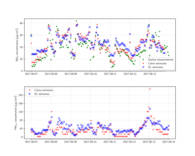
Figure 6: Time series of Caline (label data for the DL model) and DL estimates for one sample receptor over a one week time inverval. Top: NO₂ concentrations with added background values for unit-restored Caline and DL output plotted against measurements from a collocated measurement station over a 1-week time interval. Bottom: PM₁₀ concentrations for unit-restored Caline and DL output.

Last but not least, let us comment on the predictive skill of the DL model. Performance evaluation considered the ability of the DL to replicate Caline estimates at defined locations with known traffic contributions to pollution, and more broadly across the entire city with highly-varying contributions of traffic to pollution. Figure 6 presents a time-series plot of DL estimates against Caline for both NO₂ and PM₁₀ at one example receptor collocated with an NO₂ measurement site used for our validation. The neural-network closely captures the general trends of the Caline estimates, particularly the diurnal component, with (traffic-driven) higher values during the day. Differences between Caline and DL model during that period are on average less than 3 $\mu$g/cm³ for NO₂ and 15 $\mu$g/cm³ for PM₁₀, with no evident biases.

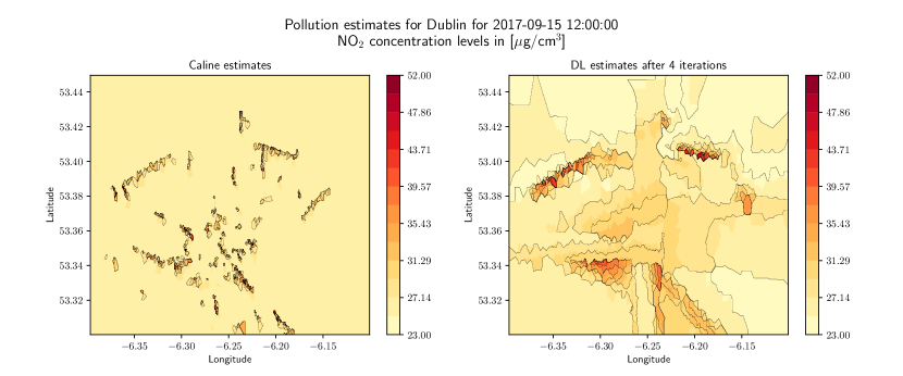
Figure 7: Spatial contour plot of modelled NO₂ estimates for selected time snapshot across the entire study domain. The partitioning of the domain into individual subdomains and the distribution of line sources of traffic volumes within those subdomains is provided in Figure 4. Left: Caline estimate. Right: Our DL estimate.

The spatial distribution of pollutants is significantly more complex, encapsulating a high dependency on local features (location of traffic line sources) together with the Gaussian-plume distribution characteristics of the Caline model. Figure 7 presents a contour map of Caline and DL estimates of NO₂ values across the entire domain at an instance in time. Results demonstrate that the DL model captures areas of high pollution contributions rather well, with peak values similar for Caline and DL. Across large areas of the model domain, Caline reports low values of traffic pollution with values falling back to an ambient level of background pollution. The DL model, on the other hand, predicts a much more uniform distribution of NO₂ concentrations, which is not as tightly restricted by the geographical proximity to traffic line sources.

This serves to illustrate one of the key differences of model estimates guided by physical rules and that driven purely by data. Caline estimates of pollution are restricted to the immediate vicinity of line-sources based on the physical equations governing the Gaussian plume model. The DL model faces no such restriction and instead seeks the optimal combinations of weights that minimise the objective functions. Results demonstrate a tendency towards a smoother distribution of pollution by the DL model compared to that produced by Caline. This results in a significant mismatch between DL and Caline estimates in regions where traffic-generated pollution is low. The mean absolute error (MAE) of the deep-learning computed values was 1.7 $\mu$g/cm³ with a standard deviation of 2.1 $\mu$g/cm³.

6 Conclusions

We have presented consistency constraints, which make it possible to train surrogate models on small domains and apply the trained models to larger domains, while allowing incorporation of information external to the domain. The consistency constraints will ensure that the solutions are physically meaningful even at the boundary of the small domains in the output of the surrogate model. We have demonstrated promising results on an air-pollution forecasting model for Dublin, Ireland.

For the first time, this work makes it possible to apply deep-learning techniques to develop surrogate models that potentially exceed the capabilities of the more complex parent model. Borrowing domain-decomposition techniques from the PDE community, it provides a framework to merge the outputs from disparate models or solutions that have spatial dependencies. In contrast, traditional machine-learning approaches consider each model prediction to be a function of events that happen within the computational domain. Numerous approaches, however, exist in the PDE literature to incorporate processes outside the domain (e.g., Dirichlet or Neumann boundary conditions, Iterative Schwarz interface methods) and are particularly common in parallel-computing implementations. This paper presents a first demonstration of implementing exchange of information across domains to a deep-learning framework. Leveraging consistency constraints, we demonstrate a deep-learning approach that learns the mapping of each domain individually and using RNN techniques, iteratively adjusts consistency constraints to provide an optimal representation of the global solution. Within the domain of our example application, recent surveys [70] also suggest that ours is the first use of deep-learning in the forecast of air-pollution levels.

This work makes possible numerous extensions. Following the copious literature on PDE-based models of air pollution, one could consider further pollutants such as ground-level ozone concentrations [71], and ensemble [72] or multi-fidelity methods. One may also consider a joint model, allowing for traffic forecasting, weather forecasting, and air-pollution forecasting, within the same network, possibly using LSTM units [73], at the same time. More generally, one could consider further applications of the consistency constraints, e.g., in energy conservation, or merging the outputs of a number of PDE models within multi-physics applications. In multi-resolution approaches, lower-resolution (e.g., city-, country-scale) component could constrain higher-resolution components (e.g., district-, city-scale), which in turn impose consistency constraints on the former. In some applications, it may be useful to explore other network topologies. Following [35], one could use long short-term memory (LSTM) units. Further, over-fitting control could be based on an improved stacked auto-encoder architecture [74]. In interpretation of the trained model, the approach of [73] may be applicable. One could also consider applications to inverse problems, following [75, 76]. Finally, one could generalise our methods in a number of directions of the multi-fidelity [55] modelling, e.g., by combining the reduced-order and full-order models using adaptation, fusion, or filtering.

Our work could also be seen as an example of Geometric Deep Learning [77], especially in conjunction with the use of mesh-free methods [38], such as the 3D point clouds [78], non-uniform meshing, or non-uniform choice of receptors within the meshes. Especially for applications, where the grids are in 3D or higher dimensions, the need for such techniques is clear. More generally, one could explore links to isogeometric analysis of [79], which integrates solving PDEs with geometric modelling. Overall, the scaling up of deep learning for PDE-based models seems to be a particular fruitful area for further research.

References

- World Health Organization [2018] World Health Organization, Burden of disease from household air pollution for 2016, WHO, Geneva, Switzerland, URL http://www.who.int/airpollution/data/HAP_BoD_results_May2018_final.pdf, 2018.
- Zhang and Batterman [2013] K. Zhang, S. Batterman, Air pollution and health risks due to vehicle traffic, Science of the total Environment 450 (2013) 307–316.
- City of London Corporation [2015] City of London Corporation, City of London Air Quality Strategy 2015–2020, Tech. Rep., City of London, 2015.
- OECD [2014] OECD, The Cost of Air Pollution, 2014.
- James et al. [2018] S. C. James, Y. Zhang, F. O’Donncha, A machine learning framework to forecast wave conditions, Coastal Engineering 137 (2018) 1–10, ISSN 0378-3839.
- Benner et al. [2015] P. Benner, S. Gugercin, K. Willcox, A survey of projection-based model reduction methods for parametric dynamical systems, SIAM Review 57 (4) (2015) 483–531.
- Goodfellow et al. [2016] I. Goodfellow, Y. Bengio, A. Courville, Deep learning, MIT Press, Cambridge, MA, 2016.
- Rumelhart et al. [1986] D. E. Rumelhart, G. E. Hinton, R. J. Williams, Learning representations by back-propagating errors, nature 323 (6088) (1986) 533.
- de Saint-Venant [1871] B. de Saint-Venant, Théorie du mouvement non permanent des eaux, avec application aux crues des rivières et a l’introduction de marées dans leurs lits, Comptes rendus de l’Académie des Sciences 16 (1871) 147–154.
- Lighthill and Whitham [1955] M. J. Lighthill, G. B. Whitham, On kinematic waves II. A theory of traffic flow on long crowded roads, Proc. R. Soc. Lond. A 229 (1178) (1955) 317–345.
- Stockie [2011] J. M. Stockie, The mathematics of atmospheric dispersion modeling, SIAM Review 53 (2) (2011) 349–372.
- Norris [1999] J. R. Norris, Smoluchowski’s coagulation equation: Uniqueness, nonuniqueness and a hydrodynamic limit for the stochastic coalescent, Annals of Applied Probability (1999) 78–109.
- Ronnie Sircar and Papanicolaou [1998] K. Ronnie Sircar, G. Papanicolaou, General Black-Scholes models accounting for increased market volatility from hedging strategies, Applied Mathematical Finance 5 (1) (1998) 45–82.
- Godunov [1959] S. K. Godunov, A difference method for numerical calculation of discontinuous solutions of the equations of hydrodynamics, Matematicheskii Sbornik 89 (3) (1959) 271–306.
- LeVeque [1990] R. J. LeVeque, Conservative methods for nonlinear problems, in: Numerical Methods for Conservation Laws, Springer, 122–135, 1990.
- Lax [1957] P. D. Lax, Hyperbolic systems of conservation laws II, Communications on pure and applied mathematics 10 (4) (1957) 537–566.
- Donea [1984] J. Donea, A Taylor–Galerkin method for convective transport problems, International Journal for Numerical Methods in Engineering 20 (1) (1984) 101–119.
- Ragnoli et al. [2019] E. Ragnoli, M. Zayats, F. O’Donncha, S. Zhuk, Localised sequential state estimation for advection dominated flows with non-Gaussian uncertainty description, Journal of Computational Physics 387 (2019) 356–375.
- O’Donncha et al. [2019a] F. O’Donncha, R. Iakymchuk, A. Akhriev, P. Gschwandtner, P. Thoman, T. Heller, X. Aguilar, K. Dichev, C. Gillan, S. Markidis, E. Laure, E. Ragnoli, V. Vassiliadisa, M. Johnston, H. Jordan, T. Fahringer, AllScale toolchain pilot applications: PDE based solvers using a parallel development environment, Computer Physics Communications (2019a) 107089.
- Quarteroni and Valli [1999a] A. Quarteroni, A. A. Valli, Domain decomposition methods for partial differential equations, Clarendon Press, ISBN 0198501781, 1999a.
- Smith et al. [2004] B. F. Smith, P. E. Bjørstad, W. Gropp, Domain decomposition : parallel multilevel methods for elliptic partial differential equations, Cambridge University Press, ISBN 0521602866, 2004.
- Lagaris et al. [1998] I. E. Lagaris, A. Likas, D. I. Fotiadis, Artificial neural networks for solving ordinary and partial differential equations, IEEE Transactions on Neural Networks 9 (5) (1998) 987–1000, ISSN 1045-9227.
- Lagaris et al. [2000] I. E. Lagaris, A. C. Likas, D. G. Papageorgiou, Neural-network methods for boundary value problems with irregular boundaries, IEEE Transactions on Neural Networks 11 (5) (2000) 1041–1049, ISSN 1045-9227.
- Lee and Kang [1990] H. Lee, I. S. Kang, Neural algorithm for solving differential equations, Journal of Computational Physics 91 (1) (1990) 110–131.
- Ramuhalli et al. [2005] P. Ramuhalli, L. Udpa, S. S. Udpa, Finite-element neural networks for solving differential equations, IEEE Transactions on Neural Networks 16 (6) (2005) 1381–1392, ISSN 1045-9227.
- Delpiano and Zegers [2006] J. Delpiano, P. Zegers, Semi-Autonomous Neural Networks Differential Equation Solver, in: The 2006 IEEE International Joint Conference on Neural Network Proceedings, ISSN 2161-4393, 1863–1869, 2006.
- Muro and Ferrari [2009] G. D. Muro, S. Ferrari, A constrained backpropagation approach to solving Partial Differential Equations in non-stationary environments, in: 2009 International Joint Conference on Neural Networks, ISSN 2161-4393, 685–689, 2009.
- Rudd et al. [2014] K. Rudd, G. D. Muro, S. Ferrari, A Constrained Backpropagation Approach for the Adaptive Solution of Partial Differential Equations, IEEE Transactions on Neural Networks and Learning Systems 25 (3) (2014) 571–584, ISSN 2162-237X.
- Rudd [2013] K. Rudd, Solving Partial Differential Equations Using Artificial Neural Networks, Ph.D. thesis, 2013.
- Brunton et al. [2019] S. L. Brunton, B. R. Noack, P. Koumoutsakos, Machine learning for fluid mechanics, Annual Review of Fluid Mechanics 52.
- Wang et al. [2019] Q. Wang, J. S. Hesthaven, D. Ray, Non-intrusive reduced order modeling of unsteady flows using artificial neural networks with application to a combustion problem, Journal of Computational Physics 384 (2019) 289 – 307, ISSN 0021-9991.
- Lary et al. [2004] D. Lary, M. Müller, H. Mussa, Using neural networks to describe tracer correlations, Atmospheric Chemistry and Physics 4 (1) (2004) 143–146.
- Loyola and Diego [2006] R. Loyola, G. Diego, Applications of neural network methods to the processing of earth observation satellite data, Neural networks 19 (2) (2006) 168–177.
- Tompson et al. [2017] J. Tompson, K. Schlachter, P. Sprechmann, K. Perlin, Accelerating Eulerian Fluid Simulation With Convolutional Networks, in: D. Precup, Y. W. Teh (Eds.), Proceedings of the 34th International Conference on Machine Learning, vol. 70 of Proceedings of Machine Learning Research, PMLR, International Convention Centre, Sydney, Australia, 3424–3433, 2017.
- Wiewel et al. [2018] S. Wiewel, M. Becher, N. Thuerey, Latent-space Physics: Towards Learning the Temporal Evolution of Fluid Flow, arXiv preprint arXiv:1802.10123 .
- Hesthaven and Ubbiali [2018] J. Hesthaven, S. Ubbiali, Non-intrusive reduced order modeling of nonlinear problems using neural networks, Journal of Computational Physics 363 (2018) 55 – 78, ISSN 0021-9991.
- Guo and Hesthaven [2019] M. Guo, J. S. Hesthaven, Data-driven reduced order modeling for time-dependent problems, Computer Methods in Applied Mechanics and Engineering 345 (2019) 75 – 99, ISSN 0045-7825.
- Sirignano and Spiliopoulos [2017] J. Sirignano, K. Spiliopoulos, DGM: A deep learning algorithm for solving partial differential equations, arXiv preprint arXiv:1708.07469 .
- Long et al. [2019] Z. Long, Y. Lu, B. Dong, PDE-Net 2.0: Learning PDEs from data with a numeric-symbolic hybrid deep network, Journal of Computational Physics 399 (2019) 108925.
- Qin et al. [2019] T. Qin, K. Wu, D. Xiu, Data driven governing equations approximation using deep neural networks, Journal of Computational Physics .
- Ray and Hesthaven [2018] D. Ray, J. S. Hesthaven, An artificial neural network as a troubled-cell indicator, Journal of Computational Physics 367 (2018) 166 – 191, ISSN 0021-9991.
- Ray and Hesthaven [2019] D. Ray, J. S. Hesthaven, Detecting troubled-cells on two-dimensional unstructured grids using a neural network, Journal of Computational Physics 397 (2019) 108845, ISSN 0021-9991.
- Chen et al. [2018] T. Q. Chen, Y. Rubanova, J. Bettencourt, D. K. Duvenaud, Neural Ordinary Differential Equations, in: S. Bengio, H. Wallach, H. Larochelle, K. Grauman, N. Cesa-Bianchi, R. Garnett (Eds.), Advances in Neural Information Processing Systems 31, Curran Associates, Inc., 6572–6583, URL http://papers.nips.cc/paper/7892-neural-ordinary-differential-equations.pdf, 2018.
- Grathwohl et al. [2019] W. Grathwohl, R. T. Q. Chen, J. Bettencourt, D. Duvenaud, Scalable Reversible Generative Models with Free-form Continuous Dynamics, in: International Conference on Learning Representations, 2019.
- Gulgec et al. [2019] N. S. Gulgec, Z. Shi, N. Deshmukh, S. Pakzad, M. Takáč, FD-Net with Auxiliary Time Steps: Fast Prediction of PDEs using Hessian-Free Trust-Region Methods, in: NeurIPS 2019 Workshop (Beyond First Order Methods in ML), 2019.
- Han et al. [2018] J. Han, A. Jentzen, E. Weinan, Solving high-dimensional partial differential equations using deep learning, Proceedings of the National Academy of Sciences 115 (34) (2018) 8505–8510.
- Thomas and Jacko [2007] S. Thomas, R. B. Jacko, Model for Forecasting Expressway Fine Particulate Matter and Carbon Monoxide Concentration: Application of Regression and Neural Network Models, Journal of the Air & Waste Management Association 57 (4) (2007) 480–488.
- Dong et al. [2009] M. Dong, D. Yang, Y. Kuang, D. He, S. Erdal, D. Kenski, PM2.5 concentration prediction using hidden semi-Markov model-based times series data mining, Expert Systems with Applications 36 (5) (2009) 9046 – 9055, ISSN 0957-4174.
- Qi et al. [2017a] Z. Qi, T. Wang, G. Song, W. Hu, X. Li, et al., Deep Air Learning: Interpolation, Prediction, and Feature Analysis of Fine-grained Air Quality, arXiv preprint arXiv:1711.00939 .
- Zhu et al. [2018] D. Zhu, C. Cai, T. Yang, X. Zhou, A Machine Learning Approach for Air Quality Prediction: Model Regularization and Optimization, Big Data and Cognitive Computing 2 (1) (2018) 5.
- Fisher [1981] M. L. Fisher, The Lagrangian relaxation method for solving integer programming problems, Management science 27 (1) (1981) 1–18.
- Bertsekas [2003] D. P. Bertsekas, Nonlinear programming, Athena Scientific, second edition, second printing., 2003.
- Gergonne [1974] J. Gergonne, The application of the method of least squares to the interpolation of sequences, Historia Mathematica 1 (4) (1974) 439–447.
- Boyd and Vandenberghe [2004] S. Boyd, L. Vandenberghe, Convex optimization, Cambridge university press, 2004.
- Peherstorfer et al. [2018] B. Peherstorfer, K. Willcox, M. Gunzburger, Survey of multifidelity methods in uncertainty propagation, inference, and optimization, SIAM Review 60 (3) (2018) 550–591.
- Cybenko [1989] G. Cybenko, Approximation by superpositions of a sigmoidal function, Mathematics of Control, Signals and Systems 2 (4) (1989) 303–314.
- Quarteroni and Valli [1999b] A. Quarteroni, A. Valli, Domain decomposition methods for partial differential equations numerical mathematics and scientific computation, Quarteroni, A. Valli–New York: Oxford University Press.–1999 .
- Nagendra and Khare [2002] S. Nagendra, M. Khare, Line source emission modelling, Atmospheric Environment 36 (13) (2002) 2083 – 2098, ISSN 1352-2310.
- Benson [1984] P. E. Benson, CALINE 4-A DISPERSION MODEL FOR PREDICTING AIR POLLUTANT CONCENTRATIONS NEAR ROADWAYS, Tech. Rep., 1984.
- United States Environmental Protection Agency [1980] United States Environmental Protection Agency, User’s guide for HIWAY – 2, Tech. Rep., 1980.
- United States Environmental Protection Agency [2003] United States Environmental Protection Agency, User’s guide for the AMS/EPA Regulatory Model (AERMOD), Tech. Rep., 2003.
- Samaranayake et al. [2014] S. Samaranayake, S. Glaser, D. Holstius, J. Monteil, K. Tracton, E. Seto, A. Bayen, Real-Time Estimation of Pollution Emissions and Dispersion from Highway Traffic, Computer-Aided Civil and Infrastructure Engineering 29 (7) (2014) 546–558.
- Scire et al. [2000] J. S. Scire, D. G. Strimaitis, R. J. Yamartino, et al., A user’s guide for the CALPUFF dispersion model .
- flu [2009] ANSYS FLUENT 12.0 User’s Guide, Tech. Rep., 2009.
- Hsu [1992] K.-J. Hsu, Time series analysis of the interdependence among air pollutants, Atmospheric Environment. Part B. Urban Atmosphere 26 (4) (1992) 491–503.
- Hossain [2014] K. Hossain, Predictive Ability of Improved Neural Network Models to Simulate Pollutant Dispersion, International Journal of Atmospheric Sciences 2014.
- US-EPA [2018] US-EPA, Air Quality Dispersion Modeling - Preferred and Recommended Models, URL https://www.epa.gov/scram/air-quality-dispersion-modeling-preferred-and-recommended-models, 2018.
- Broderick et al. [2004] B. Broderick, U. Budd, B. Misstear, S. Jennings, D. Ceburnis, Validation of Air Pollution Dispersion Modelling for the Road Transport Sector under Irish Conditions: Final Report, Tech. Rep., Project 2000-LS-6.3-M1). Environmental Protection Agency, Johnstown Castle …, 2004.
- Abadi et al. [2016] M. Abadi, et al., TensorFlow: A System for Large-scale Machine Learning, in: Proceedings of the 12th USENIX Conference on Operating Systems Design and Implementation, OSDI’16, USENIX Association, Berkeley, CA, USA, 265–283, 2016.
- Bellinger et al. [2017] C. Bellinger, M. S. M. Jabbar, O. Zaïane, A. Osornio-Vargas, A systematic review of data mining and machine learning for air pollution epidemiology, BMC public health 17 (1) (2017) 907.
- Mallet et al. [2013] V. Mallet, A. Nakonechny, S. Zhuk, Minimax filtering for sequential aggregation: Application to ensemble forecast of ozone analyses, Journal of Geophysical Research: Atmospheres 118 (19).
- O’Donncha et al. [2019b] F. O’Donncha, Y. Zhang, B. Chen, S. C. James, Ensemble model aggregation using a computationally lightweight machine-learning model to forecast ocean waves, Journal of Marine Systems 199 (2019b) 103206.
- Cui et al. [2018] Z. Cui, K. Henrickson, R. Ke, Y. Wang, High-Order Graph Convolutional Recurrent Neural Network: A Deep Learning Framework for Network-Scale Traffic Learning and Forecasting, arXiv preprint arXiv:1802.07007 .
- Zhou et al. [2017] T. Zhou, G. Han, X. Xu, Z. Lin, C. Han, Y. Huang, J. Qin, -agree AdaBoost stacked autoencoder for short-term traffic flow forecasting, Neurocomputing 247 (2017) 31–38.
- Raissi et al. [2017] M. Raissi, P. Perdikaris, G. E. Karniadakis, Machine learning of linear differential equations using Gaussian processes, Journal of Computational Physics 348 (2017) 683 – 693, ISSN 0021-9991.
- Raissi and Karniadakis [2018] M. Raissi, G. E. Karniadakis, Hidden physics models: Machine learning of nonlinear partial differential equations, Journal of Computational Physics 357 (2018) 125 – 141, ISSN 0021-9991.
- Bronstein et al. [2017] M. M. Bronstein, J. Bruna, Y. LeCun, A. Szlam, P. Vandergheynst, Geometric Deep Learning: Going beyond Euclidean data, IEEE Signal Processing Magazine 34 (4) (2017) 18–42, ISSN 1053-5888.
- Qi et al. [2017b] C. R. Qi, L. Yi, H. Su, L. J. Guibas, Pointnet++: Deep hierarchical feature learning on point sets in a metric space, in: Advances in Neural Information Processing Systems, 5099–5108, 2017b.
- Cottrell et al. [2009] J. A. Cottrell, T. J. Hughes, Y. Bazilevs, Isogeometric analysis: toward integration of CAD and FEA, John Wiley & Sons, 2009.