EFT approach to the electron Electric Dipole Moment
at the two-loop level

Abstract

The ACME collaboration has recently reported a new bound on the electric dipole moment (EDM) of the electron, $|d_{e}|<1.1\times 10^{-29}\,{\rm e\cdot cm}$ at 90$\%$ confidence level, reaching an unprecedented accuracy level. This can translate into new relevant constraints on theories beyond the SM laying at the TeV scale, even when they contribute to the electron EDM at the two-loop level. We use the EFT approach to classify these corrections, presenting the contributions to the anomalous dimension of the CP-violating dipole operators of the electron up to the two-loop level. Selection rules based on helicity and CP play an important role to simplify this analysis. We use this result to provide new bounds on BSM with leptoquarks, extra Higgs, or constraints in sectors of the MSSM and composite Higgs models. The new ACME bound pushes natural theories significantly more into fine-tune territory, unless they have a way to accidentally preserve CP.

1 Introduction

Electric dipole moments (EDM) provide one of the best indirect probes for new-physics. Since a non-zero EDM requires a violation of the CP symmetry, and the Standard Model (SM) contributions are accidentally highly suppressed, the EDM is an exceptionally clean observable to uncover beyond the SM (BSM) physics. Indeed, if BSM physics lies at the TeV scale, we expect new interactions and therefore new sources of CP violation to be present, inducing sizable EDM to be observed in the near future. For this reason, experimental bounds on the electron and neutron EDM have provided the most substantial constraints on the best motivated BSM scenarios, such as supersymmetry or composite Higgs models.

The ACME experiment has recently released a new bound on the electron EDM that improve by a factor $\sim 8.6$ their previous bound [1]:

$$|d_{e}|<1.1\cdot 10^{-29}\,{\rm e\cdot cm}\,.$$ (1.1)

This unprecedented level of accuracy allows for a sensitivity to BSM effects even if they appear at the two-loop level. Indeed, using the rough estimate,

$$\frac{d_{e}}{e}\simeq\left(\frac{g^{2}}{16\pi^{2}}\right)^{2}\frac{m_{e}}{\Lambda^{2}}\,,$$ (1.2)

we get from Eq. (1.1) a bound on the scale of new-physics $\Lambda\gtrsim 2.5$ TeV, being competitive with direct LHC searches. It is therefore of crucial interest to understand how and which BSM sectors affect the electron EDM up to the two-loop level, and which constraints can be derived from the bound Eq. (1.1).

The purpose of the paper is to use the Effective Field Theory (EFT) approach to provide a classification of the leading BSM effects on the EDM of the electron up to the two-loop level. In the EFT approach BSM indirect effects are encoded in the Wilson coefficients of higher-dimensional SM operators. At the loop level these Wilson coefficients can enter, via operator mixing, into the renormalization of the CP-violating dipole operators responsible for the EDM. By calculating the anomalous dimensions of these operators, we can provide all log-enhanced contributions to the EDM coming from new physics.

At the leading order in a $m^{2}_{W}/\Lambda^{2}$ expansion, the electron EDM arises from two dimension-6 operators, ${\cal O}_{eB}$ and ${\cal O}_{eW}$ (see below). We will present here the relevant anomalous dimensions of the imaginary part of the corresponding Wilson coefficients, $C_{eB}$ and $C_{eW}$, up to the two-loop level. In particular, we will provide the leading correction (either at the one-loop level or two-loop level) of the different Wilson coefficients $C_{i}$ to the imaginary part of $C_{eB}$ and $C_{eW}$. We will see that due to selection rules, only few Wilson coefficients enter into the renormalization of $C_{eB}$ and $C_{eW}$ at the one-loop or two-loop level. Calculating these leading corrections will allow to extract bounds on these Wilson coefficients from the recent EDM measurement.

In addition, we will also provide the most relevant one-loop anomalous dimensions of the dimension-8 operators affecting the electron EDM. Although sub-leading in the $m^{2}_{W}/\Lambda^{2}$ expansion, dimension-8 operators give contributions of order

$$\frac{d_{e}}{e}\simeq\frac{g^{2}}{16\pi^{2}}\frac{m_{e}m_{W}^{2}}{\Lambda^{4}}\,,$$ (1.3)

that can also be relevant as Eq. (1.1) leads to the bound $\Lambda\gtrsim 2$ TeV, similar to those from Eq. (1.2).

Our results can be useful to derive from Eq. (1.1) new bounds on BSM particle masses. As an example, we will provide bounds on BSM with leptoquarks or extra Higgs, showing that we can exclude masses below hundreds of TeV. We will also present constraints on new regions of the parameter space of the MSSM, as well as bounds on top-partners in composite Higgs models. These bounds can be better than those from present and future direct searches at the LHC, unless the BSM preserve CP.

2 EDM of the electron in the EFT approach

We are interested in calculating new physics contributions to the electron EDM following the EFT approach. This is a valid approximation whenever the new-physics scale $\Lambda$ is larger than the electroweak (EW) scale, such that new-physics effects on the SM can be characterized by the Wilson coefficients $C_{i}(\mu)$ of higher-dimensional SM operators. Assuming lepton number conservation, the leading effects arise from dimension-6 operators

$$\Delta{\cal L}=\sum_{i}\frac{C_{i}(\mu)}{\Lambda^{2}}{\cal O}_{i}\,,$$ (2.1)

where the Wilson coefficients are induced at the new-physics scale, $C_{i}(\mu=\Lambda)$, and must be evolved via the renormalization group equations (RGEs) down to the relevant physical scale at which the measurement takes place. Since the Wilson coefficients mix via loop effects in the RGEs, precise measurements, such as the EDM, can be sensitive to different Wilson coefficients induced by different sectors of the BSM.

The EDM of the electron is measured at low-energies $\mu\ll m_{e}$, and can then be extracted in the EFT approach from the coefficient of the operator

$$-\frac{i}{2}d_{e}(\mu)\,\bar{e}\sigma_{\mu\nu}\gamma_{5}eF^{\mu\nu}\,,$$ (2.2)

evaluated at the electron mass,

$$d_{e}=d_{e}(\mu=m_{e})\,,$$ (2.3)

where $F_{\mu\nu}$ is the field-strength of the photon. The RG evolution of $d_{e}(\mu)$ from $\Lambda$ to $m_{e}$ must be computed in the EFT made with the states lighter than $\mu$. This means that from the new-physics scale $\Lambda$ down to the EW scale we must use the SM EFT, while below the EW scale we must use the effective theory including only light SM fermions, gluons and photons. Let us start discussing the contributions to $d_{e}(\mu)$ in the SM EFT.

2.1 SM EFT basis

We will work mainly within the Warsaw basis [2], as the loop operator mixing is simpler in this basis due to the presence of many non-renormalization results. Nevertheless, we will make two changes in the four-fermion operators of the Warsaw basis. In particular, we will make the replacement

$${\cal O}^{(3)}_{lequ}=(\bar{L}_{L}^{a}\sigma_{\mu\nu}e_{R})\varepsilon_{ab}(\bar{Q}_{L}^{b}\sigma^{\mu\nu}u_{R}) \ \to\ {\cal O}_{luqe}=(\bar{L}_{L}^{a}u_{R})\varepsilon_{ab}(\bar{Q}_{L}^{b}e_{R})\,,$$ (2.4)

$${\cal O}_{le}=(\bar{L}_{L}\gamma^{\mu}L^{\prime}_{L})(\bar{e}^{\prime}_{R}\gamma_{\mu}e_{R}) \ \to\ {\cal O}_{le\bar{e}^{\prime}\bar{l}^{\prime}}=(\bar{L}_{L}e_{R})(\bar{e}^{\prime}_{R}L_{L}^{\prime})\,,$$ (2.5)

where $a,b$ denote the $\textrm{SU}(2)_{L}$ doublet indices, and $L_{L}$ and $e_{R}$ denote only the first generation lepton multiplets, while $L^{\prime}_{L}$ and $e^{\prime}_{R}$ the second and third generation ones. We also relabel the operator

$${\cal O}_{ledq}=(\bar{L}_{L}^{a}e_{R})(\bar{d}_{R}Q_{L\,a})\equiv{\cal O}_{le\bar{d}\bar{q}}\,.$$ (2.6)

Our labeling is to make clear that there are two types of operators ${\cal O}_{\psi\psi\psi\psi}$ and ${\cal O}_{\psi\psi\bar{\psi}\bar{\psi}}$ that in Weyl notation are respectively $\psi^{4}$ of total helicity 2 and $\psi^{2}\bar{\psi}^{2}$ of total helicity zero. As we will see in the following, the helicity of the operator plays a crucial role in understanding the properties of the operator mixing at the loop level [3]. In Dirac notation these two type of operators could also be written (after Fierzing) respectively as operators of type $(\bar{\Psi}\gamma_{\mu}\Psi)(\bar{\Psi}\gamma^{\mu}\Psi)$ and of type $(\bar{\Psi}_{L}\Psi_{R})(\bar{\Psi}_{L}\Psi_{R})$. In this case, for example, we would have ${\cal O}_{le\bar{d}\bar{q}}=-(\bar{L}_{L}^{a}\gamma_{\mu}Q_{L\,a})(\bar{d}_{R}\gamma^{\mu}e_{R})/2$.

tree level

${\cal O}_{eW}=(\bar{L}_{L}\sigma^{a}\sigma^{\mu\nu}e_{R})\,HW^{a}_{\mu\nu}$

${\cal O}_{eB}=(\bar{L}_{L}\sigma^{\mu\nu}e_{R})\,HB_{\mu\nu}$

1-loop

${\cal O}_{luqe}=(\bar{L}_{L}u_{R})(\bar{Q}_{L}e_{R})$

${\cal O}_{W\widetilde{W}}=|H|^{2}\,W^{a\,\mu\nu}\widetilde{W}^{a}_{\mu\nu}$

${\cal O}_{B\widetilde{B}}=|H|^{2}\,B^{\mu\nu}\widetilde{B}_{\mu\nu}$

${\cal O}_{W\widetilde{B}}=(H^{\dagger}\sigma^{a}H)\,W^{a\,\mu\nu}\widetilde{B}_{\mu\nu}$

${\cal O}_{\widetilde{W}}=\varepsilon_{abc}\widetilde{W}^{a\nu}_{\mu}W^{b\rho}_{\nu}W^{c\mu}_{\rho}$

2-loop

${\cal O}^{(1)}_{lequ}=(\bar{L}_{L}e_{R})(\bar{Q}_{L}u_{R})$

${\cal O}_{e^{\prime}W}=(\bar{L}^{\prime}_{L}\sigma^{a}\sigma^{\mu\nu}e^{\prime}_{R})\,HW^{a}_{\mu\nu}$

${\cal O}_{e^{\prime}B}=(\bar{L}^{\prime}_{L}\sigma^{\mu\nu}e^{\prime}_{R})\,HB_{\mu\nu}$

${\cal O}_{uW}=(\bar{Q}_{L}\sigma^{a}\sigma^{\mu\nu}u_{R})\,\widetilde{H}W^{a}_{\mu\nu}$

${\cal O}_{uB}=(\bar{Q}_{L}\sigma^{\mu\nu}u_{R})\,\widetilde{H}B_{\mu\nu}$

${\cal O}_{dW}=(\bar{Q}_{L}\sigma^{a}\sigma^{\mu\nu}d_{R})\,HW^{a}_{\mu\nu}$

${\cal O}_{dB}=(\bar{Q}_{L}\sigma^{\mu\nu}d_{R})\,HB_{\mu\nu}$

${\cal O}_{le\bar{d}\bar{q}}=(\bar{L}_{L}e_{R})(\bar{d}_{R}Q_{L})$

${\cal O}_{le\bar{e}^{\prime}\bar{l}^{\prime}}=(\bar{L}_{L}e_{R})(\bar{e}^{\prime}_{R}L^{\prime}_{L})$

${\cal O}_{y_{e}}=|H|^{2}\bar{L}_{L}e_{R}H$

Table 1: Operators involved in our analysis. Top-left: Operators contributing to the electron EDM at tree-level. Bottom-left: Operators contributing to the electron EDM at the one-loop level via mixing. Right: Operators contributing to the electron EDM at the two-loop level via mixing. In this table we denoted by $L_{L}$ and $e_{R}$ only the first generation lepton multiplets, while $L^{\prime}_{L}$ and $e^{\prime}_{R}$ denote the second and third generation ones.

2.2 Tree-level contributions

At tree-level there are only two dimension-6 operators that contribute to the electron EDM, namely the dipole operators ${\cal O}_{eW}$ and ${\cal O}_{eB}$, given in Table 1. We have

$$d_{e}(\mu)=\frac{\sqrt{2}v}{\Lambda^{2}}{\rm Im}\left[s_{\theta_{W}}\,C_{eW}(\mu)-c_{\theta_{W}}\,C_{eB}(\mu)\right]\,,$$ (2.7)

where we defined $v\simeq 246$ GeV as the Higgs VEV, and $s_{\theta_{W}}\equiv\sin\theta_{W}$ with $\theta_{W}$ the weak angle (similarly for the other trigonometric functions). Notice that contributions to the electron EDM arised only from the imaginary part of $C_{eW,eB}$. For this reason, we will only be interested in loop contributions to the dipole operators that can generate nonzero ${\rm Im}[C_{eW,eB}$].

2.3 One-loop effects

At the one-loop level, however, other dimension-6 operators can mix with the dipole operators ${\cal O}_{eW}$ and ${\cal O}_{eB}$, giving a contribution to $d_{e}$. Selection rules, mainly based on helicity arguments, dictate that only few operators contribute at the one-loop order to the anomalous dimension of the Wilson coefficients $C_{eW}$ and/or $C_{eB}$, as has been argued in Refs. [4, 3] based on the analysis of Ref. [5]. The relevant selection rules for our analysis are given in Table 2, where we use Weyl notation, and denote with $F$ any SM field strength, with $\psi$ any Weyl fermion and with $H$ any Higgs insertion. The ${\cal O}_{eW}$ and ${\cal O}_{eB}$ operators are of type $H\psi^{2}F$ and can then only receive contributions from operators of type $\psi^{4}$, $F^{3}$ and $H^{2}F^{2}$ of total helicity $\geq 2$.

There are four dimension-6 operators of type $\psi^{4}$, but only two contain two leptons, ${\cal O}_{luqe}$ and ${\cal O}^{(1)}_{lequ}$ given in Table 1. The second one, however, after closing the quark loop, can only give rise to the Lorentz-singlet structure $\bar{L}_{L}e_{R}$, and therefore cannot contribute to the electron dipoles. Hence only ${\cal O}_{luqe}$ contributes at the one-loop level to the anomalous dimension of ${\cal O}_{eW}$ and ${\cal O}_{eB}$. This contribution is given by

$$\frac{d}{d\ln\mu}\left(\begin{array}[]{c}C_{eB}\\ C_{eW}\end{array}\right)=\frac{y_{u}g}{16\pi^{2}}\left(\begin{array}[]{c}-\frac{1}{2}t_{\theta_{W}}N_{c}(Y_{Q}+Y_{u})\\ \frac{1}{4}N_{c}\end{array}\right)C_{luqe}\,,$$ (2.8)

where $Y_{f}$ refers to the hypercharge of the fermion $f$ ($Y_{Q}=1/6$, $Y_{u}=2/3$ and $Y_{d}=-1/3$), and $N_{c}=3$ is the number of QCD colors. Since we can work in a basis where the Yukawa matrix $y_{u}$ is diagonal, the renormalization of the imaginary part of $C_{eW,eB}$ from Eq. (2.8) only arises from the imaginary part of $C_{luqe}$.

$\curvearrowright$                        $\curvearrowright$

$F^{3}$

$\rightarrow$   $H\psi^{2}F\,,\ \psi^{4}\,,\ H^{2}F^{2}$

Table 2: Selection rules [4, 3] for the mixing at the one-loop level between the different types of dimension-6 operators (in Weyl notation).

A second type of operators, involving SM bosons, are $H^{2}F_{\mu\nu}\widetilde{F}^{\mu\nu}$. There are three operators of this type in the SM, presented in the bottom-left of Table 1. All of them contribute to the EDM at the one-loop level [6]:

$$\frac{d}{d\ln\mu}{\rm Im}\left(\begin{array}[]{c}C_{eB}\\ C_{eW}\end{array}\right)=-\frac{y_{e}g}{16\pi^{2}}\left(\begin{array}[]{ccc}0&\ \ 2t_{\theta_{W}}(Y_{L}+Y_{e})&\ \ \frac{3}{2}\\ 1&0&t_{\theta_{W}}(Y_{L}+Y_{e})\end{array}\right)\left(\begin{array}[]{c}C_{W\widetilde{W}}\\ C_{B\widetilde{B}}\\ C_{W\widetilde{B}}\end{array}\right)\,.$$ (2.9)

It is instructive to write Eq. (2.9) in a more physically oriented way, by relating the contributions to the EDM to those to the CP-violating Higgs couplings $h\gamma\gamma$, $h\gamma Z$, and to the anomalous triple gauge coupling $\delta\tilde{\kappa}_{\gamma}$, defined as

$$\frac{vh}{\Lambda^{2}}\left(\tilde{\kappa}_{\gamma\gamma}F_{\mu\nu}\widetilde{F}^{\mu\nu}+2\tilde{\kappa}_{\gamma Z}{F}_{\mu\nu}\widetilde{Z}^{\mu\nu}\right)+ie\delta\tilde{\kappa}_{\gamma}W^{+}_{\mu}W^{-}_{\nu}\widetilde{F}^{\mu\nu}\,.$$ (2.10)

We have

$$\tilde{\kappa}_{\gamma\gamma} = c^{2}_{\theta_{W}}C_{B\tilde{B}}+s^{2}_{\theta_{W}}C_{W\widetilde{W}}-c_{\theta_{W}}s_{\theta_{W}}C_{W\widetilde{B}}\,,$$

$$\tilde{\kappa}_{\gamma Z} = c_{\theta_{W}}s_{\theta_{W}}\left(C_{W\widetilde{W}}-C_{B\widetilde{B}}\right)-\frac{1}{2}(c_{\theta_{W}}^{2}-s_{\theta_{W}}^{2})C_{W\widetilde{B}}\,,$$

$$\delta\tilde{\kappa}_{\gamma} = \frac{1}{t_{\theta_{W}}}\frac{v^{2}}{\Lambda^{2}}C_{W\widetilde{B}}\,,$$ (2.11)

that, using Eq. (2.9), leads to

$$\frac{d}{d\ln\mu}d_{e}(\mu)=\frac{e}{8\pi^{2}}\frac{m_{e}}{\Lambda^{2}}\left[4Q_{e}\tilde{\kappa}_{\gamma\gamma}-\frac{4}{s_{2\theta_{W}}}\left(\frac{1}{2}+2Q_{e}s^{2}_{\theta_{W}}\right)\tilde{\kappa}_{\gamma Z}+\frac{\Lambda^{2}}{v^{2}}\delta\tilde{\kappa}_{\gamma}\right]\,,$$ (2.12)

where $Q_{e}\equiv-1/2+Y_{L}=Y_{e}=-1$ is the electric charge of the electron. Due to the approximate accidental cancellation in the electron vector coupling to the $Z$, $(1/2+2Q_{e}s^{2}_{\theta_{W}})\sim 0.04$, the main contribution to the EDM comes from $\tilde{\kappa}_{\gamma\gamma}$ and $\delta\tilde{\kappa}_{\gamma}$. In fact, this second contribution is often found to be small in many BSM scenarios, such as the MSSM or composite Higgs models, as we will see later. In these models the contribution from $\tilde{\kappa}_{\gamma\gamma}$ is the dominant one. This allows in many cases to give a direct relation between the electron EDM and the CP-violating Higgs coupling to photons.

Another class of operators that can in principle mix at the one-loop level with the electron dipole operators are other type of dipole operators $H\psi^{2}F$, for example, those involving other fermions in the SM. It is easy to see, however, that there are no possible Feynman diagrams from quark dipole operators contributing to the electron EDM at the one-loop level. For dipole operators involving other SM leptons, for example, $He\mu F$, these contributions are also absent at the one-loop level. Indeed, since we can work in a basis where the SM lepton Yukawa matrix $y_{e}$ is diagonal, none of these operators can affect the electron EDM at the one-loop level. Below we will see that there can be, however, contributions at the two-loop level.

Finally, there are operators of type $F^{3}$ that could potentially mix with the dipole operators. In the SM there are two of these operators, either with gluons (${\cal O}_{\widetilde{G}}$) or $W^{a}$ bosons (${\cal O}_{\widetilde{W}}$). The ${\cal O}_{\widetilde{G}}$ operator obviously can not give corrections to the electron dipole operators at one-loop or two-loop level, as there are no possible Feynman diagrams at these orders. On the other hand, the ${\cal O}_{\widetilde{W}}$ operator can contribute to the ${\cal O}_{eW}$ dipole at one loop. It turns out, however, that this contribution is finite, so it does not induce a running for the dipole operator. The finite contribution can be readily computed in dimensional regularization, leading to the result [7]

$${\rm Im}[C_{eW}]=\frac{3}{64\pi^{2}}y_{e}g^{2}C_{\widetilde{W}}\,.$$ (2.13)

2.4 Two-loop effects

At the two-loop level, more dimension-6 operators can contribute to the electron EDM by mixing with the dipoles ${\cal O}_{eW}$ and ${\cal O}_{eB}$. We remark that we are only interested in calculating two-loop effects for those Wilson coefficients that did not mix with the EDM operators at the loop level. We are interested in extracting bounds to their corresponding Wilson coefficients and therefore we are only interested in calculating the leading correction to the EDM. For Wilson coefficients affecting the EDM already at the one-loop level, such as $C_{luqe}$, the two-loop corrections would only provide a small correction to their bound.

New dimension-6 operators can contribute to the electron EDM by mixing with the dipoles ${\cal O}_{eW}$ and ${\cal O}_{eB}$ in two different ways. Either by mixing at the one-loop level with the operators we discussed in the previous section, ${\cal O}_{luqe}$ and ${\cal O}_{V\tilde{V}}$ ($V=W,B$), that contribute at the one-loop level to the dipoles, or by direct two-loop contribution to the anomalous dimension of ${\cal O}_{eW}$ and ${\cal O}_{eB}$ (see Table 1).

The first case can potentially give larger corrections, as in the leading-log approximation, they will contain two logarithms, i.e. $\propto\ln^{2}(\Lambda^{2}/m_{W}^{2})$. From the selection rules of Table 2, we see that only two classes of operators can contribute at this order. One is given by the $\psi^{4}$ operators that could not generate an electron dipole at the one-loop due to the absence of Feynman diagrams, namely the ${\cal O}^{(1)}_{lequ}$ operator. The second class is given by dipole operators involving the second and third lepton generations, ${\cal O}_{e^{\prime}W}$ and ${\cal O}_{e^{\prime}B}$, or the quarks, ${\cal O}_{uW}$, ${\cal O}_{uB}$, ${\cal O}_{dW}$ and ${\cal O}_{dB}$.

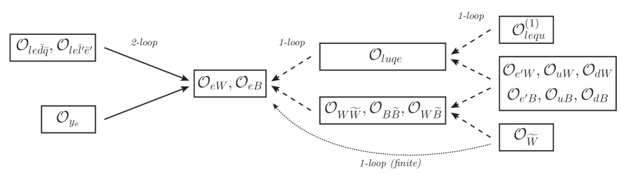
Figure 1: Corrections to the electron EDM (imaginary part of $C_{eW,eB}$) induced up to the 2-loop level. The dashed and solid arrows denote mixing at 1-loop and 2-loop order respectively. On the right we list the operators that generate contributions enhanced by a double logarithm (showing the 1-loop mixing patterns that generate it), whereas on the left we list operators giving rise to a single logarithm.

Notice that, as we pointed out before, there is an exception to the selection rules of Table 2, corresponding to a possible mixing of $\bar{\psi}^{2}\psi^{2}$ operators into $\psi^{4}$ when the pair of Yukawas either $y_{u}y_{e}$ or $y_{u}y_{d}$ is involved in the loop [4, 3]. Nevertheless, by working in the basis in which the lepton and up-type quark Yukawa matrices are real and diagonal, one can easily find that there are not $\bar{\psi}^{2}\psi^{2}$ operators contributing to the imaginary part of ${\cal O}_{luqe}$ at the one-loop level. Indeed, in this basis $y_{u}y_{e}$ is real and diagonal, and the only $\bar{\psi}^{2}\psi^{2}$ operators that could contribute to ${\cal O}_{luqe}$ are the ones involving two electron fields and two same-generation quarks. The Wilson coefficients of these operators are necessarily real and do not induce CP-violating effects.

Therefore the one-loop mixing pattern and RGEs are the following. The ${\cal O}_{lequ}$ operator can mix with ${\cal O}_{luqe}$ at the one-loop level [6]:

$$\frac{d}{d\ln\mu}C_{luqe}=\frac{g^{2}}{16\pi^{2}}\left[4(Y_{L}+Y_{e})(Y_{Q}+Y_{u})t^{2}_{\theta_{W}}-3\right]C^{(1)}_{lequ}\,.$$ (2.14)

The dipole operators, on the other hand, mix with the ${\cal O}_{luqe}$ operator, [6]

$$\frac{d}{d\ln\mu}C_{luqe}=\frac{g\,y_{e}}{16\pi^{2}}\Big{[}-8t_{\theta_{W}}(Y_{L}+Y_{e})C_{uB}+12C_{uW}\Big{]}\,,$$ (2.15)

as well as with ${\cal O}_{V\widetilde{V}}$ operators [9]:

$$\frac{d}{d\ln\mu}C_{W\widetilde{W}}=-\frac{2g}{16\pi^{2}}{\rm Im}\Big{[}y_{e^{\prime}}\,C_{e^{\prime}W}+y_{u}N_{c}\,C_{uW}+y_{d}N_{c}\,C_{dW}\Big{]}\,,$$ (2.16)

$$\frac{d}{d\ln\mu}C_{B\widetilde{B}}=-\frac{4g^{\prime}}{16\pi^{2}}{\rm Im}\Big{[}y_{e^{\prime}}(Y_{L}+Y_{e})\,C_{e^{\prime}B}+y_{u}N_{c}(Y_{Q}+Y_{u})\,C_{uB}+y_{d}N_{c}(Y_{Q}+Y_{d})\,C_{dB}\Big{]}\,,$$ (2.17)

$$\frac{d}{d\ln\mu}C_{W\widetilde{B}} = -\frac{2g}{16\pi^{2}}{\rm Im}\Big{[}2t_{\theta_{W}}\big{(}y_{e^{\prime}}(Y_{L}+Y_{e})\,C_{e^{\prime}W}-y_{u}N_{c}(Y_{Q}+Y_{u})\,C_{uW}+y_{d}N_{c}(Y_{Q}+Y_{d})\,C_{dW}\big{)}$$ (2.18)

$$\hskip 47.50006pt+\,y_{e^{\prime}}\,C_{e^{\prime}B}-y_{u}N_{c}\,C_{uB}+y_{d}N_{c}\,C_{dB}\Big{]}\,.$$

Flavor indices are easily understood as we can always work with diagonal Yukawa matrix $y_{e}$ and either $y_{u}$ or $y_{d}$.

The operator $\mathcal{O}_{\widetilde{W}}$ also enters at two loops via renormalization of the ${\cal O}_{V\tilde{V}}$ operators [6],

$$\frac{d}{d\ln\mu}C_{W\widetilde{W}}=-\frac{1}{16\pi^{2}}15g^{3}C_{\widetilde{W}}\ ,\hskip 28.45274pt\frac{d}{d\ln\mu}C_{W\widetilde{B}}=+\frac{1}{16\pi^{2}}6{g^{\prime}}g^{2}Y_{H}C_{\widetilde{W}}\,.$$ (2.19)

This leads to a two loop, double log contribution to the electron EDM, to be compared with the finite contribution at one loop in Eq. (2.13). The two loop contribution becomes comparable to the one-loop one already for $\Lambda\sim 10~{}\text{TeV}$.

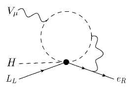
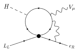
Figure 2: Feynman contributions to the anomalous dimension of ${\cal O}_{eW}$ and ${\cal O}_{eB}$ at the two-loop level from ${\cal O}_{y_{e}}$ (left) and ${\cal O}_{le\bar{d}\bar{q}}$,${\cal O}_{le\bar{e}^{\prime}\bar{l}^{\prime}}$ (right).

Let us now discuss those dimension-6 operators that can directly contribute at the two-loop level to the anomalous dimension of the electron dipole operators. In fact, we are only interested in the EDM, i.e. the imaginary part of the the dipole operators, and therefore only complex Wilson coefficients can contribute, as the SM interactions preserve CP up to small Yukawa couplings that we neglect. This reduces the list of possible dimension-6 operators to those to the right of Table 1. For example, operators of the type $\bar{\Psi}\gamma_{\mu}\Psi H^{\dagger}D^{\mu}H$ are Hermitian (and then have real Wilson coefficients) unless the two fermions involved are different, meaning that they must involve different flavors. But since in the SM we can work in the basis where $y_{e}$ and either $y_{u}$ or $y_{d}$ are diagonal, we cannot draw any two-loop Feynman diagram contributing to the electron EDM operators.

Similar conclusions can be obtained for four-fermion operators, except for those in Table 1, namely ${\cal O}_{le\bar{d}\bar{q}}$ and ${\cal O}_{le\bar{e}^{\prime}\bar{l}^{\prime}}$. There is however an important subtlety related to these operators, which results in an ambiguity in the determination of their contributions to the electron EDM.

Within the basis we are using, in which ${\cal O}_{le\bar{d}\bar{q}}$ and ${\cal O}_{le\bar{e}^{\prime}\bar{l}^{\prime}}$ are written as the product of scalar currents, it is simple to check that the $1$-loop contributions to the electron EDM trivially vanish due to the tensor structure. However, through a Fierz rearrangement, ${\cal O}_{le\bar{d}\bar{q}}$ and ${\cal O}_{le\bar{e}^{\prime}\bar{l}^{\prime}}$ can also be rewritten in the form $(\bar{\Psi}\gamma_{\mu}\Psi)(\bar{\Psi}\gamma^{\mu}\Psi)$, i.e. as a product of vector currents. With this choice, if dimensional regularization (in particular the $\overline{\rm MS}$ scheme) is used to compute the contributions to the electron EDM, a finite $1$-loop effect is found. The origin of this contribution is related to the presence of additional four-fermion interactions involving multiple gamma matrices that are generated at intermediate steps of the calculation. These are known as “evanescent operators” (for a review, see for example [10]). The coefficients of these interactions carry an $\epsilon=4-d$ factor, but they can give finite effects in the presence of $1/\epsilon$ poles. As an example, we report the contributions to the electron EDM induced by the ${\cal O}_{\ell e}=C_{\ell e}(\bar{L}_{L}\gamma^{\mu}L^{\prime}_{L})(\bar{e}^{\prime}_{R}\gamma_{\mu}e_{R})$ operator (see for instance [11, 12])

$$\frac{d_{e}}{e}=2\frac{m_{\ell^{\prime}}}{16\pi^{2}}{\rm Im}\,C_{\ell e}\,.$$ (2.20)

A similar result is obtained for the ${\cal O}_{le\bar{d}\bar{q}}$ operator in vector-current form.

Summarizing the above discussion, one finds that the contributions from the ${\cal O}_{le\bar{d}\bar{q}}$ and ${\cal O}_{le\bar{e}^{\prime}\bar{l}^{\prime}}$ $4$-fermion operators crucially depend on the choice of the operator basis and on the regularization procedure. This, in turn, can affect the matching from a UV model. In particular, finite $1$-loop contributions can be shifted from the matching to the $4$-fermion operators into the EDM operators ${\cal O}_{eB}$ and ${\cal O}_{eW}$ and vice versa. As already mentioned, for our analysis we choose the scalar-current form for the $4$-fermion operators, $(\bar{L}_{L}e_{R})(\bar{\Psi}\Psi)$. Therefore no finite one-loop contributions arise for the electron EDM from the ${\cal O}_{le\bar{d}\bar{q}}$ and ${\cal O}_{le\bar{e}^{\prime}\bar{l}^{\prime}}$ operators. As we will see in sec. 3.2.3, this choice is particularly convenient for studying UV models including heavy Higgs-like states, in which case only scalar-current $4$-fermion operators are obtained from the matching.

We have then only ${\cal O}_{y_{e}}$, ${\cal O}_{le\bar{d}\bar{q}}$ and ${\cal O}_{le\bar{e}^{\prime}\bar{l}^{\prime}}$ giving a two-loop mixing with the electric dipole operators. From ${\cal O}_{y_{e}}$ (see left-hand side of Fig. 2), we obtain

$$\frac{d}{d\ln\mu}\left(\begin{array}[]{c}C_{eB}\\ C_{eW}\end{array}\right)=\frac{g^{3}}{(16\pi^{2})^{2}}\frac{3}{4}\left(\begin{array}[]{c}t_{\theta_{W}}Y_{H}+4t^{3}_{\theta_{W}}Y_{H}^{2}(Y_{L}+Y_{e})\\ \frac{1}{2}+\frac{2}{3}t^{2}_{\theta_{W}}Y_{H}(Y_{L}+Y_{e})\end{array}\right)C_{y_{e}}\,,$$ (2.21)

while from ${\cal O}_{le\bar{d}\bar{q}}$ and ${\cal O}_{le\bar{e}^{\prime}\bar{l}^{\prime}}$ (see right-hand side of Fig. 2), we get respectively

$$\frac{d}{d\ln\mu}\left(\begin{array}[]{c}C_{eB}\\ C_{eW}\end{array}\right)=\frac{y_{d}g^{3}}{(16\pi^{2})^{2}}\frac{N_{c}}{4}\left(\begin{array}[]{c}3t_{\theta_{W}}Y_{Q}+4t_{\theta_{W}}^{3}(Y_{L}+Y_{e})(Y_{Q}^{2}+Y_{d}^{2})\\ \frac{1}{2}+2t_{\theta_{W}}^{2}(Y_{L}+Y_{e})Y_{Q}\end{array}\right)C_{le\bar{d}\bar{q}}$$ (2.22)

and

$$\frac{d}{d\ln\mu}\left(\begin{array}[]{c}C_{eB}\\ C_{eW}\end{array}\right)=\frac{y_{e^{\prime}}g^{3}}{(16\pi^{2})^{2}}\frac{1}{4}\left(\begin{array}[]{c}3t_{\theta_{W}}Y_{L}+4t_{\theta_{W}}^{3}(Y_{L}+Y_{e})(Y_{L}^{2}+Y_{e}^{2})\\ \frac{1}{2}+2t_{\theta_{W}}^{2}(Y_{L}+Y_{e})Y_{L}\end{array}\right)C_{le\bar{e}^{\prime}\bar{l}^{\prime}}\,.$$ (2.23)

We summarize our results by schematically presenting in Fig. 1 the mixing patterns of the effective operators contributing to the electron dipoles at 2-loop order. For completeness we also include the 2-loop mixing of the ${\cal O}_{\widetilde{W}}$ operator, which, at 1-loop order, only induces finite corrections to the electron dipoles. We also provide below the leading-log approximation to the electron EDM that can be good enough since the new physics scale is not constrained yet to be far away from the electroweak scale, and therefore we do not need to resum the logs by exactly solving the RGEs. We find that the one-loop corrections are

$$\frac{d_{e}}{e}\simeq-\frac{1}{16\pi^{2}}\frac{\sqrt{2}v}{\Lambda^{2}}\left[y_{u}\,{\rm Im}\,C_{luqe}-y_{e}\left(2\tilde{\kappa}_{\gamma\gamma}+\frac{1-4s_{\theta_{W}}^{2}}{s_{\theta_{W}}c_{\theta_{W}}}\tilde{\kappa}_{\gamma Z}-\frac{\Lambda^{2}}{2v^{2}}\delta\tilde{\kappa}_{\gamma}\right)\right]\ln\frac{\Lambda^{2}}{m_{h}^{2}}\,.$$ (2.24)

The double-log 2-loop corrections are given by

$$\displaystyle\frac{d_{e}}{e} \displaystyle\simeq\frac{1}{(16\pi^{2})^{2}}\frac{\sqrt{2}v}{\Lambda^{2}}\frac{1}{8}{\rm Im}\Bigg{[}\!\! \displaystyle gy_{e}\Big{(}y_{e^{\prime}}(11+9t_{\theta_{W}}^{2})c_{e^{\prime}W}+15y_{u}(3+t_{\theta_{W}}^{2})C_{uW}+3y_{d}(3+t_{\theta_{W}}^{2})C_{dW}\Big{)}$$ (2.25)

$$-\,3\frac{g}{t_{\theta_{W}}}y_{e}\Big{(}y_{e^{\prime}}(1+7t_{\theta_{W}}^{2})c_{e^{\prime}B}-3y_{u}(1+7t_{\theta_{W}}^{2})C_{uB}+y_{d}(3+5t_{\theta_{W}}^{2})C_{dB}\Big{)}$$

$$+\,2g^{2}y_{u}(3+5t_{\theta_{W}}^{2})C^{(1)}_{lequ}\,+\,y_{e}g^{3}\left(13+3\tan\theta_{W}^{2}\right)C_{\widetilde{W}}\Bigg{]}\ln^{2}\frac{\Lambda^{2}}{m_{h}^{2}}\,.$$

Finally, the single-log 2-loop corrections are

$$\frac{d_{e}}{e}\simeq-\frac{g^{2}}{(16\pi^{2})^{2}}\frac{\sqrt{2}v}{\Lambda^{2}}{\rm Im}\left[\frac{3}{8}t_{\theta_{W}}^{2}\,C_{y_{e}}+y_{d}\frac{1}{8}t_{\theta_{W}}^{2}C_{le\bar{d}\bar{q}}+y_{e^{\prime}}\frac{1}{8}\left(2+9t_{\theta_{W}}^{2}\right)C_{le\bar{e}^{\prime}\bar{l}^{\prime}}\right]\ln\frac{\Lambda^{2}}{m_{h}^{2}}\,.$$ (2.26)

Notice that we did not include in the above formula finite corrections that can arise at the matching scales. In fact, few other dimension-6 operators can enter in this way into the renormalization of the electron EDM. As we saw in Sec. 2.3, an example is provided by the ${\cal O}_{\widetilde{W}}$ operator, whose dominant corrections to the electron EDM arise as finite one-loop contributions. An analogous result is valid for the $H^{3}\bar{f}f$ operator ($f=u,d,e^{\prime}$) that modify the quarks and heavy lepton Yukawa couplings. These operators start to contribute to the electron EDM at the two-loop level through finite Barr–Zee-type diagrams [14]. We will discuss these operators in Sec. 2.6.

2.5 Dimension-8 operators

Since we are calculating corrections to the EDM at the two-loop level coming from dimension-6 operators, it is appropriate to ask whether dimension-8 operators can also give similar contributions. The effects of these operators are suppressed with respect to dimension-6 operators by an extra $m_{W}^{2}/\Lambda^{2}$, but this could be overcome if their contributions to the EDM arises at the one-loop level instead of two-loops. We will only be interested here in dimension-8 operators that can be generated from integrating new physics at tree-level and that have not been constrained from previous dimension-6 operators. For example, dimension-8 operators involving extra $|H|^{2}$ or extra derivatives will not be relevant. We only find two of these operators,

$${\cal O}_{ldqe}=(\bar{L}_{L}d_{R}H)(\bar{Q}_{L}e_{R}H)\ ,\ \ \ \ \ {\cal O}_{le^{\prime}l^{\prime}e}=(\bar{L}_{L}e_{R}^{\prime}H)(\bar{L}_{L}^{\prime}e_{R}H)\,,$$ (2.27)

that at the one-loop level can mix with dimension-8 operators of dipole type,

$${\cal O}_{h^{2}eW}=|H|^{2}{\cal O}_{eW}\ ,\ \ \ \ \ {\cal O}_{h^{2}eB}=|H|^{2}{\cal O}_{eB}\,,$$ (2.28)

similarly to Eq. (2.8):

$$\frac{d}{d\ln\mu}\left(\begin{array}[]{c}C_{h^{2}eB}\\ C_{h^{2}eW}\end{array}\right)=\frac{y_{d}g}{16\pi^{2}}\left(\begin{array}[]{c}-\frac{1}{2}t_{\theta_{W}}N_{c}(Y_{Q}+Y_{d})\\ \frac{1}{4}N_{c}\end{array}\right)C_{ldqe}\,,$$ (2.29)

and equivalently for $C_{le^{\prime}l^{\prime}e}$ with the replacement $y_{d}\to y_{e}$, $Y_{Q}\to Y_{L}$ and $Y_{d}\to Y_{e}$. We get a contribution to EDM of order

$$\frac{d_{e}}{e}\simeq-\frac{\sqrt{2}v^{3}}{\Lambda^{4}}\frac{y_{d}{\rm Im}[C_{ldqe}]}{16\pi^{2}}\frac{N_{c}}{24}\ln\frac{\Lambda^{2}}{m_{W}^{2}}\,.$$ (2.30)

2.6 Threshold effects at the EW scale: the impact of CP-violating Yukawa’s

The log-enhanced contributions we considered in the previous sections are expected to give the dominant corrections to the electron EDM. Nevertheless, being this logarithm not always so large, there are cases in which finite corrections can be more important. A noticeable example, that we will discuss here, is the case of two-loop corrections to the EDM generated when integrating out the top and the Higgs at the EW scale. These corrections come from CP-violating Yukawa couplings induced by the SM dimension-6 operator ${\cal O}_{y_{f}}$ at the EW scale:

$$c_{f}h\bar{f}_{L}f_{R}\ ,\ \ \ \ c_{f}=\frac{v^{2}}{\sqrt{2}\Lambda^{2}}C_{y_{f}}\,.$$ (2.31)

For the particular case of $C_{y_{e}}$ we obtain, from Barr–Zee diagrams, that these contributions are given by

$$\frac{d_{e}}{e}\simeq-\frac{16}{3\sqrt{2}}\frac{e^{2}}{(16\pi^{2})^{2}}v\left(2+\ln\frac{m_{t}^{2}}{m_{h}^{2}}\right)\frac{{\rm Im}\,C_{y_{e}}}{\Lambda^{2}}\,,$$ (2.32)

where we only kept the leading corrections due to diagrams with a virtual photon and a top loop. Contributions from a virtual $Z$-boson are highly suppressed by the small vector $Z$ coupling to the electron, whereas diagrams involving light quarks are suppressed by the light quark Yukawa’s. Diagrams involving a virtual $W$ boson are expected to be subleading with respect to the photon contribution, although not negligible. For simplicity we however neglect these contribution as often done in the literature. Notice that in the above formula we only included the leading terms in an expansion for large $m_{t}^{2}/m_{h}^{2}$, which reproduce the full result with an accuracy $\sim 10\%$. The appearance of $\ln m_{t}^{2}/m_{h}^{2}$ in Eq. (2.32) can be understood as a RG running of the electron EDM from the top mass, where the top is integrated out generating a $hF^{\mu\nu}F_{\mu\nu}$ term at the one-loop level, down to the Higgs mass. In particular, this arises from a loop diagram involving $hF^{\mu\nu}F_{\mu\nu}$ and the CP-violating Yukawa Eq. (2.31).

Comparing the result in Eq. (2.32) with the two-loop running in Eq. (2.26), we find that the former is typically dominant and is a factor of few larger than the latter for a cut-off scale in the $10\;$TeV range. This is because the contributions of Eq. (2.26) are slightly smaller than the naive estimate since they are proportional to $g^{\prime}$ and are suppressed by an accidental factor $3/8$. The two contributions become comparable only for a very large cut-off scale $\sim 10^{4}\;$TeV.

Similarly, $C_{y_{u,d}}$ and $C_{y_{e^{\prime}}}$, which can give CP-violating corrections to the quark and to the heavy lepton Yukawa’s, can lead to finite Barr–Zee contributions to the electron EDM. For the top case, we have

$$\frac{d_{e}}{e}\simeq-\frac{e^{2}}{(16\pi^{2})^{2}}2\sqrt{2}N_{c}Q_{t}^{2}\frac{m_{e}}{m_{t}}v\left(2+\ln\frac{m_{t}^{2}}{m_{h}^{2}}\right)\frac{{\rm Im}\,C_{y_{t}}}{\Lambda^{2}}\,.$$ (2.33)

Again, the $\ln m_{t}^{2}/m_{h}^{2}$ can be understood as a RG running of the electron EDM from the top mass, where a $hF\tilde{F}$ term is generated from the CP-violating top Yukawa after integrating out the top, down to the Higgs mass.

2.7 EFT below the electroweak scale and relevant RGEs

Let us now discuss the RG running effects below the EW scale. At the scale $\mu\sim m_{W}$, we must integrate out all the heavy SM particles, the $W$, $Z$, the Higgs and top, and work for $\mu<m_{W}$ with the EFT built with the light fermions, the photon and the gluons. The EDM of the electron arises in this EFT from a dimension-5 operator

$${\cal O}_{e\gamma}=\bar{e}_{L}\sigma^{\mu\nu}e_{R}F_{\mu\nu}\,,$$ (2.34)

whose coefficient, from the tree-level matching with the SM EFT at the EW scale, is given by

$$C_{e\gamma}(m_{W})=\frac{v}{\sqrt{2}\Lambda}\left(s_{\theta_{W}}\,C_{eW}(m_{W})-c_{\theta_{W}}\,C_{eB}(m_{W})\right)+\frac{v^{3}}{2\sqrt{2}\Lambda^{3}}\left(s_{\theta_{W}}\,C_{h^{2}eW}(m_{W})-c_{\theta_{W}}\,C_{h^{2}eB}(m_{W})\right)\,.$$ (2.35)

Other relevant operators below the EW scale are four-fermion operators made with the light SM fermions. The matching at the EW scale is given by

$$C_{luqe}(m_{W}){\cal O}_{luqe} = C_{euue}(m_{W})(\bar{e}_{L}u_{R})(\bar{u}_{L}e_{R})+\cdots\,,$$

$$C^{(1)}_{lequ}(m_{W}){\cal O}^{(1)}_{lequ} = C_{eeuu}(m_{W})(\bar{e}_{L}e_{R})(\bar{u}_{L}u_{R})+\cdots\,,$$

$$C_{le\bar{d}\bar{q}}(m_{W}){\cal O}_{le\bar{d}\bar{q}} = C_{ee\bar{d}\bar{d}}(m_{W})(\bar{e}_{L}e_{R})(\bar{d}_{R}d_{L})+\cdots\,,$$

$$C_{le\bar{e}\bar{l}}(m_{W}){\cal O}_{le\bar{e}\bar{l}} = C_{le\bar{e}\bar{e}}(m_{W})(\bar{e}_{L}e_{R})(\bar{e}^{\prime}_{R}e^{\prime}_{L})+\cdots\,,$$ (2.36)

and

$$C_{ldqe}(m_{W}){\cal O}_{ldqe} = \frac{v^{2}}{2\Lambda^{2}}C_{edde}(m_{W})(\bar{e}_{L}d_{R})(\bar{d}_{L}e_{R})+\cdots\,,$$

$$C_{le^{\prime}l^{\prime}e}(m_{W}){\cal O}_{le^{\prime}l^{\prime}e} = \frac{v^{2}}{2\Lambda^{2}}C_{ee^{\prime}e^{\prime}e}(m_{W})(\bar{e}_{L}e^{\prime}_{R})(\bar{e}^{\prime}_{L}e_{R})+\cdots\,,$$

$$C_{ldqe}(m_{W}){\cal O}_{leqd} = \frac{v^{2}}{2\Lambda^{2}}C_{eedd}(m_{W})(\bar{e}_{L}e_{R})(\bar{d}_{L}d_{R})+\cdots\,,$$

$$C_{le^{\prime}l^{\prime}e}(m_{W}){\cal O}_{lel^{\prime}e^{\prime}} = \frac{v^{2}}{2\Lambda^{2}}C_{eee^{\prime}e^{\prime}}(m_{W})(\bar{e}_{L}e_{R})(\bar{e}^{\prime}_{L}e^{\prime}_{R})+\cdots\,,$$ (2.37)

where we have also included the matching of the dimension-8 SM operators

$${\cal O}_{leqd}=(\bar{L}_{L}e_{R}H)(\bar{Q}_{L}d_{R}H)\ ,\ \ \ \ \ {\cal O}_{lel^{\prime}e^{\prime}}=(\bar{L}_{L}e_{R}H)(\bar{L}_{L}^{\prime}e^{\prime}_{R}H)\,.$$ (2.38)

The above four-fermion operators can enter into the anomalous dimension of ${\cal O}_{e\gamma}$ at the one or two loop level. Using our previous results, we can easily extract the RGE for $C_{e\gamma}$ since the renormalization of the photon can be read from that of the ${\rm U}(1)_{Y}$-boson in the SM. At the one-loop level we only have, equivalently to Eq. (2.8) and Eq. (2.29), (see also [15])

$$\frac{d}{d\ln\mu}C_{e\gamma}=-\frac{e}{16\pi^{2}}\frac{1}{\sqrt{2}}\left(\frac{m_{u}}{\Lambda}N_{c}Q_{u}C_{euue}+\frac{m_{d}v^{2}}{2\Lambda^{3}}N_{c}Q_{d}C_{edde}+\frac{m_{e^{\prime}}v^{2}}{2\Lambda^{3}}Q_{e}C_{ee^{\prime}e^{\prime}e}\right)\,,$$ (2.39)

where $Q_{f}$ refers to the EM charge of the fermion $f$. At the two-loop level, we can have contribution to $C_{e\gamma}$ either by a one-loop mixing of ${\cal O}_{eeff}$ with ${\cal O}_{effe}$ ($f=u,d,e^{\prime}$), similarly to Eq. (2.14),

$$\frac{d}{d\ln\mu}C_{effe}=\frac{e^{2}}{\pi^{2}}Q_{e}Q_{f}C_{eeff}\,,$$ (2.40)

or by a direct contribution to $C_{e\gamma}$:

$$\frac{d}{d\ln\mu}C_{e\gamma}=\frac{e^{3}}{(16\pi^{2})^{2}}\left(\frac{m_{d}}{\Lambda}4N_{c}Q_{e}Q^{2}_{d}C_{ee\bar{d}\bar{d}}+\frac{m_{e}}{\Lambda}4Q_{e}^{3}C_{ee^{\prime}\bar{e}^{\prime}\bar{e}}\right)\,.$$ (2.41)

The RGE running should be considered from $m_{W}$ down to the mass of the heaviest fermion in the four-fermion operator, where the state should be integrated out. Therefore this running can be important for lighter fermions.

We can compare our results with those obtained from Barr-Zee diagrams arising from CP-violating Yukawa interactions Eq. (2.31). For light quarks and leptons $e^{\prime}$, one finds respectively

$$\frac{d_{e}}{e}\simeq-\frac{e^{2}}{(16\pi^{2})^{2}}4N_{c}Q_{q}^{2}v\frac{m_{e}m_{q}}{m_{h}^{2}}\left(\ln^{2}\frac{m_{q}^{2}}{m_{h}^{2}}+\frac{\pi^{2}}{3}\right)\frac{{\rm Im}\,C_{y_{q}}}{\Lambda^{2}}\,,$$ (2.42)

and

$$\frac{d_{e}}{e}\simeq-\frac{e^{2}}{(16\pi^{2})^{2}}4Q_{e}^{2}v\frac{m_{e}m_{e^{\prime}}}{m_{h}^{2}}\left(\ln^{2}\frac{m_{e^{\prime}}^{2}}{m_{h}^{2}}+\frac{\pi^{2}}{3}\right)\frac{{\rm Im}\,C_{y_{e^{\prime}}}}{\Lambda^{2}}\,.$$ (2.43)

The double logarithm in Eqs. (2.42) and (2.43) can be understood from an EFT perspective as the RG running from the Higgs mass, where integrating the Higgs generates a complex $C_{eeff}$ from Eq. (2.31), down to the light fermion masses. The relevant RGEs are indeed those in Eq. (2.39) and Eq. (2.40).

For light quarks, however, a better bound on the corresponding Wilson coefficient can be obtained from constraints on CP-violating electron-nucleon interactions, that the ACME collaboration has also recently reported [1]:

$$-\frac{G_{F}}{\sqrt{2}}i\bar{e}\gamma_{5}e\bar{N}\left(C^{(0)}_{S}+C^{(1)}_{S}\sigma_{3}\right)N\ ,\ \ \ \ C_{S}=C_{S}^{(0)}+\frac{Z-N}{Z+N}C_{S}^{(1)}<7.3\cdot 10^{-10}\,.$$ (2.44)

Neglecting isospin breakings that in the ThO are small [1], we have for the down-quarks

$$C_{S}\simeq C_{S}^{(0)}=-\frac{{\rm Im}[C_{ee\bar{d}\bar{d}}]}{\sqrt{2}G_{F}\Lambda^{2}}\langle N|\bar{d}d|N\rangle\,.$$ (2.45)

We have checked that bounds from $d_{e}$ are slightly better than those from $C_{S}$ for operators involving the bottom (using $\langle N|\bar{b}b|N\rangle\simeq 74$ MeV$/m_{b}$ [16]), while the bound from $C_{S}$ is better for ligher quarks.

3 Impact on BSM

3.1 Power counting of the Wilson coefficients

So far we have presented the leading contributions of the dimension-6 operators to the anomalous dimension of the electron electric dipole operators up to two loops. All the possible contributing operators are given in Table 1. Nevertheless, the importance of the different operators depends on the size of their Wilson coefficients, which crucially depends on the BSM dynamics.

In the following we will be interested in BSM theories that can be described as weakly-coupled renormalizable theories. These includes all possible extensions of the SM with extra particles with renormalizable interactions. In these BSM theories we can classify the Wilson coefficients as those that can be generated at tree-level and those generated at most at the loop level. For example, among the operators of Table 1, the only ones with Wilson coefficients that can be induced at tree-level by integrating out new heavy states are all the four-fermion operators and ${\cal O}_{y_{e}}$; the rest, involving always field-strengths, can only be generated by loops. Therefore, we expect

$$C_{fV}\sim\frac{g_{*}^{3}g}{16\pi^{2}}\ ,\ \ \ C_{V\widetilde{V}}\sim\frac{g^{2}_{*}g^{2}}{16\pi^{2}}\ ,\ \ \ C_{luqe},C_{lequ},C_{le\bar{d}\bar{q}},C_{le\bar{e}^{\prime}\bar{l}^{\prime}},C_{y_{e}}\sim g^{2}_{*}\,,$$ (3.1)

where $g_{*}$ refers to a generic coupling of the BSM dynamics to the SM, $f=e,u,d$ and $V=W,B$.

${\cal O}_{luqe}$	Scalar $\bf(3,2,7/6)$
	Scalar $\bf(\bar{3},1,1/3)$
${\cal O}^{(1)}_{lequ}$	Scalar $\bf(1,2,1/2)$
	Scalar $\bf(\bar{3},1,1/3)$
${\cal O}_{le\bar{d}\bar{q}}$	Vector $\bf(\bar{3},2,5/6)$
	Vector $\bf(3,1,2/3)$
	Scalar $\bf(1,2,1/2)$
${\cal O}_{le\bar{e}^{\prime}\bar{l}^{\prime}}$	Vector $\bf(1,1,0)$
	Vector $\bf(1,2,1/2)$
	Scalar $\bf(1,2,1/2)$

${\cal O}_{y_{e}}$	Fermion $\bf(1,2,-1/2)\oplus(1,1(3),-1)$
	Fermion $\bf(1,2,-1/2)\oplus(1,1(3),0)$
	Fermion $\bf(1,2,-3/2)\oplus(1,1(3),0)$
	Scalar $\bf(1,2,1/2)$

Table 3: States transforming under the SM group ${\rm SU}(3)_{c}\times{\rm SU}(2)_{L}\times{\rm U}(1)_{Y}$ contributing at the tree-level to the operators of Table 1.

In this class of BSM theories the contributions to the electron EDM have the following loop expansion. The leading contributions are of order $d_{e}/e\sim(g_{*}^{2}/16\pi^{2})(m_{u}/\Lambda^{2})\ln({\Lambda/m_{W}})$ and can arise from those particular BSM that contribute to ${\cal O}_{luqe}$ at tree-level. There are only two types of particles that can generate ${\cal O}_{luqe}$ at tree-level (see Table 3), the leptoquarks $R_{2}$ and $S_{1}$ that will be discussed below.

Next, we can have BSM dynamics contributing directly to the Wilson coefficients of the electron dipole operators, that can give corrections of one-loop order (but without a log-enhancement), $d_{e}/e\sim(g_{*}^{2}/16\pi^{2})(g_{*}v/\Lambda^{2})$. This can happen in BSM theories that contain fermions and bosons coupled to the electron, with at least one of them charged, as for example, the selectron and wino in supersymmetric theories.

Contributing at the two-loop level, we have those BSM theories inducing ${\cal O}^{(1)}_{lequ}$ at tree-level, which leads to a double-log enhanced EDM, $d_{e}/e\sim g^{2}g_{*}^{2}/(16\pi^{2})^{2}(m_{u}/\Lambda^{2})\ln^{2}({\Lambda/m_{W}})$. As shown in Table 3, this includes BSM theories with extra Higgses.

Single-log two-loop contributions can come from BSM scenarios generating ${\cal O}_{V\tilde{V}}$ at the loop level (those BSM containing extra charged fermions coupled to the Higgs), or generating ${\cal O}_{le\bar{d}\bar{q}}$, ${\cal O}_{le\bar{e}^{\prime}\bar{l}^{\prime}}$ or ${\cal O}_{y_{e}}$ at tree-level (see Table 3). Also BSM theories generating ${\cal O}_{luqe}$ at one-loop level can lead to a single-log two-loop contribution to the electron EDM, as we will see later for the case of the MSSM.

Finally, BSM theories with extra ${\rm SU(2)}_{L}$ fermions can generate ${\cal O}_{\widetilde{W}}$ at the loop-level, leading to a contribution to the electron EDM at the two-loop level with no log enhancement. On the other hand, BSM theories contributing to the EDM of a fermion different from the electron are expected to give negligible effects to the electron EDM, as these arise at best at the three-loop level.

Examples of these classes of BSM theories will be given below. We must also notice that there is a large class of low-energy effective descriptions of strongly-coupled theories that follow the same power counting described above. These are those theories that were assumed to follow the ”minimal coupling” assumption [17], and correspond to holographic models as well as their deconstructed versions.

It is also important to keep in mind that operators of Table 1 containing the fields $\bar{L}_{L}$ and $e_{R}$ can potentially give a contribution to the electron mass. This places a constraint on the natural size of their Wilson coefficients. In particular, we find

$$\left\{\frac{C_{eV}\,v}{16\pi^{2}}\ ,\ \frac{C_{y_{e}}\,v^{3}}{\Lambda^{2}}\ ,\ \frac{C_{lequ}\,m_{u}}{16\pi^{2}}\ ,\ \frac{C_{luqe}\,m_{u}}{16\pi^{2}}\ ,\ \frac{C_{le\bar{d}\bar{q}}\,m_{d}}{16\pi^{2}}\ ,\ \frac{C_{le\bar{e}\bar{l}}\,m_{e^{\prime}}}{16\pi^{2}}\right\}\lesssim m_{e}\,.$$ (3.2)

In fact, in most of the UV-complete BSM theories (e.g. supersymmetry, composite Higgs or theories with flavor symmetries only broken by Yukawas) we expect operators with chirality flips to carry yukawa couplings, i.e.,

$$C_{fV}\propto y_{f}\ ,\ \ \ C_{y_{e}}\propto y_{e}\ ,\ \ \ C_{lequ}\propto y_{e}y_{u}\ ,\ \ \ C_{luqe}\propto y_{e}y_{u}\ ,\ \ \ C_{le\bar{d}\bar{q}}\propto y_{e}y_{d}\ ,\ \ \ C_{le\bar{e}^{\prime}\bar{l}^{\prime}}\propto y_{e}y_{e^{\prime}}\,,$$ (3.3)

implying that we only expect sizable contributions to the electron EDM from four-fermion operators involving the third family. All these considerations can be useful for a proper interpretation of the recent ACME bound.

tree-level
$C_{eW}$	$5.5\times 10^{-5}\,y_{e}g$
$C_{eB}$	$5.5\times 10^{-5}\,y_{e}g^{\prime}$
one-loop
$C_{luqe}$	$1.0\times 10^{-3}\,y_{e}y_{t}$
$C_{W\widetilde{W}}$	$4.7\times 10^{-3}\,g^{2}$
$C_{B\widetilde{B}}$	$5.2\times 10^{-3}\,g^{\prime\,2}$
$C_{W\widetilde{B}}$	$2.4\times 10^{-3}\,gg^{\prime}$
$C_{\widetilde{W}}$	$6.4\times 10^{-2}\,g^{3}$

two-loops
$C_{lequ}$	$3.8\times 10^{-2}\,y_{e}y_{t}$
$C_{\tau W}$	$260\,y_{\tau}g$
$C_{\tau B}$	$380\,y_{\tau}g^{\prime}$
$C_{tW}$	$6.9\times 10^{-3}\,y_{t}g$
$C_{tB}$	$1.2\times 10^{-2}\,y_{t}g^{\prime}$
$C_{bW}$	$64\,y_{b}g$
$C_{bB}$	$47\,y_{b}g^{\prime}$
$C_{le\bar{d}\bar{q}}$	$10\,y_{e}y_{t}(y_{t}/y_{b})$
$C_{le\bar{e}^{\prime}\bar{l}^{\prime}}$	$0.63\,y_{e}y_{t}(y_{t}/y_{\tau})$

two-loops finite
$C_{y_{e}}$	$20\,y_{e}\lambda_{h}$
$C_{y_{t}}$	$20\,y_{t}\lambda_{h}$
$C_{y_{b}}$	$4.1\times 10^{3}\,y_{b}\lambda_{h}$
$C_{y_{\tau}}$	$4.8\times 10^{3}\,y_{\tau}\lambda_{h}$

Table 4: Bounds on the Wilson coefficients coming from Eq. (1.1) taking $\Lambda=10$ TeV. For a better appreciation of the bound, we have extracted the Yukawa, gauge or Higgs coupling ($\lambda_{h}=0.1$) that we naturally expect to carry these Wilson coefficients. For $C_{le\bar{d}\bar{q}}$ and $C_{le\bar{e}^{\prime}\bar{l}^{\prime}}$ we have further extracted a factor $(y_{t}/y_{b})$ and $(y_{t}/y_{\tau})$ respectively to reflect the fact that these coefficients can be potentially larger consistently with their natural sizes Eq. (3.2).

In Table 4 we list the bounds on individual Wilson coefficients that can be inferred from the new electron EDM measurement Eq. (1.1). To derive the bounds we considered the various Wilson coefficients one-by-one. Although typical BSM theories give rise to simultaneous contributions to several Wilson coefficients, strong cancellations are typically not present. In such situation the bounds obtained on single Wilson coefficients remain approximately valid.

3.2 Leptoquarks and extra Higgs

As a first example of an application of the above EFT analysis, we focus here on new-physics models containing states of Table 3. In particular, we focus on leptoquarks and heavy Higgs-like states.

As can be seen from Table 3, four leptoquark multiplets can give rise to electron EDM contributions up to two-loop order. Among scalar leptoquarks only the $R_{2}$ and the $S_{1}$ multiplets give rise to contributions to $d_{e}$. In both cases the contributions arise at one-loop level and include a logarithmically-enhanced term. On the other hand, vector leptoquarks, in particular the $V_{2}$ and the $U_{1}$ multiplets can contribute to the electron EDM at one-loop order only with finite contributions.

We analyze the various cases in the following, providing the matching with the EFT operators in the limit of heavy multiplet masses. For the scalar leptoquarks, we also compare the leading running contributions to the EDM with the full results, which are already known in the literature. For simplicity we only include couplings to third-generation quarks, since interactions with the light generations give rise to EDM contributions suppressed by the light-fermion Yukawa couplings.

3.2.1 Scalar leptoquarks

We start our discussion with the case of scalar leptoquarks.

The $R_{2}$ leptoquark

The first case we consider is the $R_{2}$ multiplet, whose ${\rm SU}(3)_{c}\times{\rm SU}(2)_{L}\times{\rm U}(1)_{Y}$ quantum numbers are $({\bf 3},{\bf 2},{\bf 7/6})$. The Lagrangian describing the relevant leptoquark interactions with the SM fermions is

$${\cal L}=-y_{2}^{RL}\overline{t}_{R}R^{a}\varepsilon^{ab}L^{b}_{L_{1}}+y_{2}^{LR}\overline{e}_{R}R^{a*}Q^{a}_{L_{3}}+{\rm h.c.}\,,$$ (3.4)

where $L_{L_{i}}$ and $Q_{L_{i}}$ labels the $i$-generation lepton and quark respectively. In the limit of large mass, the $R_{2}$ leptoquark gives rise to a contribution to the ${\cal O}_{luqe}$ effective operator, namely

$${\cal L}_{\it eff}^{R_{2}}=\frac{y_{2}^{LR*}y_{2}^{RL*}}{m_{R_{2}}^{2}}{\cal O}_{luqe}+{\rm h.c.}\,.$$ (3.5)

Using Eq. (2.24), we can obtain the log-enhanced one-loop contribution to the electron EDM:

$$\frac{d_{e}}{e}\simeq\frac{1}{8\pi^{2}}\frac{m_{t}}{m_{R_{2}}^{2}}{\rm Im}\left(y_{2}^{LR}y_{2}^{RL}\right)\ln\frac{m_{R_{2}}^{2}}{m_{t}^{2}}\,.$$ (3.6)

The full one-loop contribution to the electron EDM is also known in the literature[22]

$$\frac{d_{e}}{e}=\frac{3}{32\pi^{2}}\frac{m_{t}}{m_{R_{2}}^{2}}{\rm Im}\left(y_{2}^{LR}y_{2}^{RL}\right)\left[Q_{t}I_{2}\left(m_{t}^{2}/m_{R_{2}}^{2}\right)+Q_{LQ}J_{2}\left(m_{t}^{2}/m_{R_{2}}^{2}\right)\right]\,,$$ (3.7)

where $Q_{t}=2/3$ and $Q_{LQ}=5/3$ are the electric charges of the top quark and $R_{2}$ leptoquark, while the $I_{2}$ and $J_{2}$ functions are given by

$$I_{2}(x)=\frac{1}{(1-x)^{3}}(-3+4x-x^{2}-2\ln x)\,,\qquad J_{2}(x)=\frac{1}{(1-x)^{3}}(1-x^{2}+2x\ln x)\,.$$ (3.8)

One can easily check that the leading logarithmic term in Eq. (3.8) agrees with the result of the EFT calculation in Eq. (3.6). In fact, the leading-log contribution in Eq. (3.6) provides a quite good approximation of the full result even for relatively small leptoquark masses. The discrepancy is below $25\%$ for $m_{R_{2}}>300\;{\rm GeV}$ and below $10\%$ for $m_{R_{2}}>360\;{\rm GeV}$.

The recent bound on the electron EDM Eq. (1.1) translates into the constraint

$$m_{R_{2}}\gtrsim 420\;{\rm TeV}\,\sqrt{\frac{|{\rm Im}(y_{2}^{LR}y_{2}^{RL})|}{y_{e}y_{t}}\left(1+0.075\ln\frac{|{\rm Im}(y_{2}^{LR}y_{2}^{RL})|}{y_{e}y_{t}}\right)}\,,$$ (3.9)

where we have normalized $y_{2}^{LR}y_{2}^{RL}$ to the electron and top Yukawa coupling, following the estimates presented in Eq. (3.3).

The $S_{1}$ leptoquark

The second leptoquark state that can give rise to one-loop contributions to the electron EDM is the $S_{1}$ multiplet, which has $({\bf\overline{3}},{\bf 1},{\bf 1/3})$ quantum numbers. Its interactions with the SM fermions can be parametrized by

$${\cal L}=y_{1}^{LL}\overline{Q}_{L_{3}}^{C\,a}S_{1}\varepsilon^{ab}L_{L_{1}}^{b}+y_{1}^{RR}\overline{t}_{R}S_{1}e_{R}+{\rm h.c.}\,,$$ (3.10)

where the $C$ superscript denotes the charge conjugation operation, namely $\psi^{C}\equiv C\overline{\psi}^{T}$ with $C=i\gamma^{2}\gamma^{0}$. Integrating out $S_{1}$ gives rise to a contribution to ${\cal O}_{luqe}$ and ${\cal O}^{(1)}_{\ell equ}$, namely

$${\cal L}_{\it eff}^{S_{1}}=\frac{y_{1}^{LL*}y_{1}^{RR}}{m_{S_{1}}^{2}}\left[{\cal O}_{luqe}+{\cal O}^{(1)}_{lequ}\right]+{\rm h.c.}\,.$$ (3.11)

Therefore, from Eq. (2.24), we obtain the following log-enhanced one-loop contribution to the electron EDM

$$\frac{d_{e}}{e}\simeq\frac{1}{8\pi^{2}}\frac{m_{t}}{m_{S_{1}}^{2}}{\rm Im}\left(y_{1}^{LL}y_{1}^{RR*}\right)\ln\frac{m_{S_{1}}^{2}}{m_{t}^{2}}\,.$$ (3.12)

The full one-loop result reads [20]

$$\frac{d_{e}}{e}=\frac{1}{32\pi^{2}}\frac{m_{t}}{m_{S_{1}}^{2}}{\rm Im}\left(y_{1}^{LL}y_{1}^{RR*}\right)G\left({m_{t}^{2}}/{m_{S_{1}}^{2}}\right)\,,$$ (3.13)

where the $G$ function is defined by

$$G(x)=\frac{1}{(1-x)^{3}}\left(5-8x+3x^{2}+2(2-x)\ln x\right)\,.$$ (3.14)

We find that the leading-log approximation in Eq. (3.12) is in fair agreement with the full result, the difference being $\lesssim 30\%$ for $m_{S_{1}}\gtrsim 220\;{\rm GeV}$.

Eq. (1.1) translates into the bound

$$m_{S_{1}}\gtrsim 400\;{\rm TeV}\,\sqrt{\frac{|{\rm Im}(y_{1}^{LL}y_{1}^{RR*})|}{y_{e}y_{t}}\left(1+0.081\ln\frac{|{\rm Im}(y_{1}^{LL}y_{1}^{RR*})|}{y_{e}y_{t}}\right)}\,.$$ (3.15)

3.2.2 Vector leptoquarks

We now consider the case of vector leptoquarks. Before specializing the discussion to the $V_{2}$ and $U_{1}$ cases, we discuss some generic features of these models.

As we already mentioned, vector leptoquarks can give rise to a finite contribution to the electron EDM at the $1$-loop order. In order to compute the EDM effects, one needs first of all to embed the vector leptoquark into a well-behaved (i.e. renormalizable) UV theory. For this purpose one can consider GUT-like extensions of the SM, as done in refs. [23, 24], which always lead to the following Lagrangian for the couplings of the Leptoquark $V_{\mu}$ to the photon $A_{\mu}$

$${\cal L}\supset-i\,e\,Q_{V}\left[(\partial_{\mu}V_{\nu}^{\dagger}-\partial_{\nu}V_{\mu}^{\dagger})A^{\mu}V^{\nu}-(\partial_{\mu}V_{\nu}-\partial_{\nu}V_{\mu})A^{\mu}V^{\nu\dagger}+(V_{\mu}V_{\nu}^{\dagger}-V_{\nu}V_{\mu}^{\dagger})\partial^{\mu}A^{\nu}\right]\,,$$ (3.16)

where $Q_{V}$ is the leptoquark electric charge. The couplings of a vector leptoquark to the electron and a quark $q$ can be parametrized as

$$\mathcal{L}\supset g_{L}\bar{e}_{L}\gamma^{\mu}q_{L}V_{\mu}+g_{R}\bar{e}_{R}\gamma^{\mu}q_{R}V_{\mu}+{\rm h.c.}\,.$$ (3.17)

The $1$-loop contribution to the electron EDM is given by

$$\frac{d_{e}}{e}=\frac{N_{c}(Q_{V}-Q_{q})}{8\pi^{2}}\frac{m_{q}}{m_{V}^{2}}\text{Im}(g_{L}g_{R}^{\star})\,,$$ (3.18)

where $m_{q}$ and $Q_{q}$ are the mass and the electric charge of the quark, while $m_{V}$ is the leptoquark mass. Notice that contributions come from two type of diagrams, one in which the photon is attached to the quark line and one in which it is attached to the leptoquark line. The two contributions are therefore proportional to $Q_{q}$ ad $Q_{V}$ respectively.

Within our EFT description, these contributions must be matched directly into the Wilson coefficients $C_{eW}$ and $C_{eB}$ at the scale $m_{V}$. Notice, however, that the leptoquark gives also rise to effective $4$-fermion interactions of the form $(\bar{L}_{L}^{a}\gamma_{\mu}Q_{L\,a})(\bar{b}_{R}\gamma^{\mu}e_{R})$ that after Fierzing leads to ${\cal O}_{le\bar{d}\bar{q}}$. As we discussed, the ${\cal O}_{le\bar{d}\bar{q}}$ operator however do not contribute at $1$-loop to the electron EDM but at the $2$-loop order.

The $V_{2}$ leptoquark

Let us now consider $V_{2}$ multiplet with quantum numbers $({\bf\overline{3}},{\bf 2},{\bf 5/6})$. The relevant interactions with the SM fermions read

$${\cal L}=x_{2}^{RL}\overline{b}_{R}^{C}\gamma^{\mu}V^{a}_{2,\mu}\varepsilon^{ab}L_{L_{1}}^{b}+x_{2}^{LR}\overline{Q}_{L_{3}}^{C\,a}\gamma^{\mu}\varepsilon^{ab}V^{b}_{2,\mu}e_{R}+{\rm h.c.}\,.$$ (3.19)

Using the above formulae we find the following $1$-loop contribution to the electron EDM

$$\frac{d_{e}}{e}=-\frac{5}{8\pi^{2}}\frac{m_{b}}{m_{V_{2}}^{2}}\text{Im}(x_{2}^{LR}x_{2}^{RL\star})\,.$$ (3.20)

The new bound from the ACME collaboration leads to

$$m_{V_{2}}\gtrsim 5.5\,\text{TeV }\,\sqrt{\frac{\text{Im}(x_{2}^{LR}x_{2}^{RL\star})}{y_{e}y_{b}}}\,.$$ (3.21)

The $U_{1}$ leptoquark

The second possible vector leptoquark that gives a contributions to the electron EDM is the $U_{1}$ state, with quantum numbers $({\bf 3},{\bf 1},{\bf 2/3})$. Its Lagrangian reads

$${\cal L}=x_{1}^{LL}\overline{Q}_{L_{3}}^{a}\gamma^{\mu}U_{1,\mu}L^{a}_{L_{1}}+x_{1}^{RR}\overline{b}_{R}\gamma^{\mu}U_{1,\mu}e_{R}+{\rm h.c.}\,.$$ (3.22)

The $1$-loop contributions to the electron EDM are given by .

$$\frac{d_{e}}{e}=-\frac{1}{8\pi^{2}}\frac{m_{b}}{m_{U_{1}}^{2}}\text{Im}(x_{2}^{RR}x_{2}^{LL\star})\,.$$ (3.23)

The bound in Eq. (1.1) leads to

$$m_{U_{1}}\gtrsim 2.5\,\text{TeV }\,\sqrt{\frac{\text{Im}(x_{2}^{RR}x_{2}^{LL\star})}{y_{e}y_{b}}}\,.$$ (3.24)

3.2.3 The Heavy Higgs

The last type of massive multiplets we consider are Higgs-like states $H$ with quantum numbers $({\bf 1},{\bf 2},{\bf 1/2})$. Depending on their allowed couplings to the SM fermions they can give rise to different sets of contributions to the electron EDM.

In general a Higgs-like multiplet can have couplings to all SM fermion species. For simplicity we consider only couplings to the electron family and to third generation fermions, discarding flavor-violating couplings. We parametrize the relevant heavy Higgs interactions as

$${\cal L}=\kappa_{e}{H}^{a}\overline{L}_{L_{1}}^{a}e_{R}+\kappa_{t}\widetilde{H}^{a}\overline{Q}_{L_{3}}^{a}t_{R}+\kappa_{b}{H}^{a}\overline{Q}_{L_{3}}^{a}b_{R}+\kappa_{\tau}{H}^{a}\overline{L}_{L_{3}}^{a}\tau_{R}+\eta(H^{\dagger}h)|h|^{2}+{\rm h.c.}\,,$$ (3.25)

where $\widetilde{H}^{a}\equiv\varepsilon^{ab}{H}^{b*}$ and $h$ denotes here the SM Higgs doublet. In the limit of heavy mass, integrating out the Higgs-like state gives rise to three effective operators that contribute to the electron EDM, namely

$${\cal L}_{\it eff}^{H}=-\frac{\kappa_{e}\kappa_{t}}{m_{H}^{2}}{\cal O}^{(1)}_{lequ}+\frac{\kappa_{e}\kappa_{b}^{*}}{m_{H}^{2}}{\cal O}_{le\bar{d}\bar{q}}+\frac{\kappa_{e}\kappa_{\tau}^{*}}{m_{H}^{2}}{\cal O}_{le\bar{\tau}\bar{l}}+\frac{\kappa_{e}\eta}{m_{H}^{2}}{\cal O}_{y_{e}}\,,$$ (3.26)

where ${\cal O}_{le\tau l}=(\overline{L}_{L_{1}}^{a}e_{R})(\overline{\tau}_{R}L_{L_{3}}^{a})$. As we saw in the previous sections all the effective operators in Eq. (3.26) give rise to a contribution to the electron EDM at two-loop order. There are however some important differences. The ${\cal O}^{(1)}_{lequ}$ operator can potentially lead to the largest contribution, since its effects are enhanced by a double logarithm. The remaining two operators lead instead to the single logarithmic.

The leading contributions to the electron EDM from the four effective operators are given respectively by

$$\frac{d_{e}}{e}\simeq\frac{3g^{2}+5g^{\prime 2}}{2(16\pi^{2})^{2}}\frac{m_{t}}{m_{H}^{2}}{\rm Im}(\kappa_{e}\kappa_{t})\ln^{2}\frac{m_{H}^{2}}{m_{t}^{2}}\,\,,$$ (3.27)

$$\frac{d_{e}}{e}\simeq-\frac{4}{(16\pi^{2})^{2}}\frac{m_{b}}{m_{H}^{2}}{\rm Im}\left(\kappa_{e}\kappa_{b}^{*}\right)\left[\frac{e^{2}}{3}\ln\frac{m_{H}^{2}}{m_{b}^{2}}+g^{Z}_{e}g^{Z}_{b}\ln\frac{m_{H}^{2}}{m_{Z}^{2}}-\frac{g^{2}}{16}\ln\frac{m_{H}^{2}}{m_{W}^{2}}\right]\,,$$ (3.28)

$$\frac{d_{e}}{e}\simeq-\frac{4}{(16\pi^{2})^{2}}\frac{m_{\tau}}{m_{H}^{2}}{\rm Im}\left(\kappa_{e}\kappa_{\tau}^{*}\right)\left[e^{2}\ln\frac{m_{H}^{2}}{m_{\tau}^{2}}+(g^{Z}_{e})^{2}\ln\frac{m_{H}^{2}}{m_{Z}^{2}}+\frac{g^{2}}{16}\ln\frac{m_{H}^{2}}{m_{W}^{2}}\right]\,,$$ (3.29)

and

$$\frac{d_{e}}{e}\simeq-\frac{3g^{2}t_{\theta_{W}}^{2}}{8(16\pi^{2})^{2}}\frac{\sqrt{2}v}{m_{H}^{2}}{\rm Im}\left(\kappa_{e}\eta\right)\ln\frac{m_{H}^{2}}{m_{h}^{2}}\,.$$ (3.30)

These two-loop results agree with the Barr–Zee results [14, 25].

The new bound on the electron EDM leads to the constraints

$$m_{H}\gtrsim 66\;{\rm TeV}\,\sqrt{\frac{|{\rm Im}(\kappa_{e}\kappa_{t})|}{y_{e}y_{t}}}\left(1+0.11\ln\frac{|{\rm Im}(\kappa_{e}\kappa_{t})|}{y_{e}y_{t}}\right)\,,$$ (3.31)

$$m_{H}\gtrsim 0.88\;{\rm TeV}\,\sqrt{\frac{|{\rm Im}(\kappa_{e}\kappa_{b})|}{y_{e}y_{t}}\left(1+0.036\ln\frac{|{\rm Im}(\kappa_{e}\kappa_{b})|}{y_{e}y_{t}}\right)}\,,$$ (3.32)

and

$$m_{H}\gtrsim 1.4\;{\rm TeV}\,\sqrt{\frac{|{\rm Im}(\kappa_{e}\kappa_{\tau})|}{y_{e}y_{t}}\left(1+0.092\ln\frac{|{\rm Im}(\kappa_{e}\kappa_{\tau})|}{y_{e}y_{t}}\right)}\,,$$ (3.33)

for a Higgs coupling to top, bottom and tau respectively. In the presence of a non-vanishing $\eta$, the contribution to the CP-violating electron Yukawa leads to the additional bound

$$m_{H}\gtrsim 4.9\;{\rm TeV}\,\sqrt{\frac{|{\rm Im}(\kappa_{e}\eta)|}{y_{e}}\left(1+0.18\ln\frac{|{\rm Im}(\kappa_{e}\eta)|}{y_{e}}\right)}\,.$$ (3.34)

Notice that this bound, for $\eta\sim 1$, is significantly stronger than the ones derived in the presence of couplings to the bottom or $\tau$, but is much weaker than the one expected in the presence of a sizeable coupling to the top quark.

3.3 The MSSM

We will work within the MSSM assuming that the superpartner masses are larger than the EW scale. CP-violating phases can appear in several terms of the MSSM. Either in the supersymmetric parameter $\mu$ (that corresponds to the Higgsino mass), or in soft supersymmetry breaking terms: Bino and Wino masses, $M_{1}$ and $M_{2}$ respectively, Higgs mixing mass term, $m^{2}_{12}H_{u}H_{d}$, and the scalar trilinears, e.g. $y_{u}A_{u}H_{u}\widetilde{Q}_{L}\tilde{u}_{R}$. Nevertheless, only those combinations of MSSM parameters whose phase cannot be removed by redefinitions of fields can lead to physical CP-violating effects. A recent analysis of the impact of the new ACME bound on the MSSM can be found in Ref. [26].

The main contribution from the MSSM arise from one-loop contributions to $C_{eW}$ and $C_{eB}$, that generate an electron EDM calculated long ago -see for example [27]. From Winos and left-handed selectrons ($\tilde{L}_{L}$), we have

$$\frac{d_{e}}{e}\simeq-\frac{g^{2}}{16\pi^{2}}\frac{m_{e}}{m_{\tilde{L}_{L}}^{2}}\tan\beta\frac{\text{Im}(M_{2}\mu)}{|M_{2}|^{2}-|\mu|^{2}}\left[I_{2}\left(\frac{M_{2}^{2}}{m_{\tilde{L}_{L}}^{2}}\right)-I_{2}\left(\frac{\mu^{2}}{m_{\tilde{L}_{L}}^{2}}\right)\right]\,,$$ (3.35)

where $I_{2}$ is defined in Eq. (3.8). These effects are generated at $\Lambda\sim$ mass of the superpartners. Taking $\tan\beta\sin({\rm Arg}[\mu M_{2}])\sim 1$, we get from the new bound Eq. (1.1)

$$m_{\tilde{L}_{L}}\gtrsim 25\,(50)\ {\rm TeV}\,,$$ (3.36)

for $m_{\tilde{L}_{L}}=M_{2}=\mu$ ($m_{\tilde{L}_{L}}\gg\mu=M_{2}$).

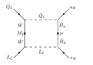
Figure 3: Feynman diagram of the MSSM contribution to ${\cal O}_{luqe}$.

At the two-loop order, we can get contributions from other regions of the parameter space of the MSSM. For example, Wino-Higgsino loops can induce the Wilson coefficients $C_{W\widetilde{W}},C_{B\widetilde{B}},C_{W\widetilde{B}}$ (the Bino contribution is much smaller for $M_{1}\sim M_{2}$), that, contrary to the one-loop Eq. (3.35), do not involve a $\tilde{L}_{L}$. These are give by

$$C_{W\widetilde{W}} = C_{loop}\,\frac{-8+27\rho-24\rho^{2}+5\rho^{3}+6\rho^{2}\ln\rho}{16(\rho-1)^{3}}\,,$$

$$C_{B\widetilde{B}} = t_{\theta_{W}}^{2}C_{loop}\,\frac{\rho(11-16\rho+5\rho^{2}-2(\rho-4)\ln\rho)}{16(\rho-1)^{3}}\,,$$

$$C_{W\widetilde{B}} = t_{\theta_{W}}C_{loop}\,\frac{\rho(7-8\rho+\rho^{2}+2(\rho+2)\ln\rho)}{8(\rho-1)^{3}}\,,$$ (3.37)

where $\rho\equiv|M_{2}/\mu|^{2}$ and

$$C_{loop}\equiv\frac{g^{4}\sin 2\beta\sin\varphi}{16\pi^{2}|M_{2}\mu|}\ ,\ \ \varphi={\rm Arg}[m^{2}_{12}\mu^{*}M_{2}^{*}]\,.$$ (3.38)

Using Eq. (3.37) and Eq. (2.12), we can obtain the contribution to the electron EDM in agreement with Ref. [28] in the large log-approximation. From the ACME bound Eq. (1.1), we get a limit on the Wino and Higgsino masses that can be approximately written as

$$\sqrt{|M_{2}\mu|}\gtrsim 4\,{\rm TeV}\,,$$ (3.39)

where we have taken $\sin 2\beta\sim\sin\varphi\sim 1$.

Another type of two-loop contributions to the electron EDM can arise from one-loop contributions to $C_{luqe}$. From loops involving selectrons, squarks, Winos and Higgsinos (see Fig. 3), we have

$${\rm Im}\,C_{luqe}=-y_{e}y_{u}\frac{3g^{2}\,{\rm Im}[\mu M_{2}]}{16\pi^{2}\sin 2\beta}F(m^{2}_{i})\,,$$ (3.40)

where

$$F(m^{2}_{i})=-\sum_{i}\frac{m^{2}_{i}\ln m^{2}_{i}}{\Pi_{i\not=j}(m^{2}_{i}-m^{2}_{j})},$$ (3.41)

with $i$ running over the mass of the Higgsino, Wino, $\tilde{u}_{R}$ and $\tilde{L}_{L}$. These results are valid for any quark generation $u\to u,c,t$. For equal superpartner masses, we have $F(m^{2}_{i})=1/(12m_{i}^{4})$, and Eq. (2.24) and the ACME bound lead to

$$m_{i}\gtrsim 7.5\,{\rm TeV}\,,$$ (3.42)

for $\sin({\rm Arg}[\mu M_{2}])/\sin 2\beta\sim 1$. Notice that, contrary to Eq. (3.35) and Eq. (3.38), the $\sin 2\beta$ appears in Eq. (3.40) in the denominator and therefore becomes larger for small values of $\tan\beta$.

3.4 Composite Higgs

As a last example we consider the class of composite Higgs models. For definiteness we focus on minimal scenarios based on the $\textrm{SO}(5)\rightarrow\textrm{SO}(4)$ symmetry breaking pattern, which gives rise to a single Higgs doublet [29]. Depending on the implementation of the flavor structure different contributions to the electron EDM can arise. In models based on the anarchic partial compositeness paradigm naively extended to both quark and lepton sectors [30], large contributions arise at the one-loop level due to the presence of partners of the SM leptons and/or composite vector resonances. These contributions are generated at the mass scale of the composite states and can be estimated as [31, 32]

$$\frac{d_{e}}{e}\sim\frac{1}{8\pi^{2}}\frac{m_{e}}{f^{2}}\,,$$ (3.43)

where $f$ denotes the Goldstone Higgs decay constant (or equivalently the scale of spontaneous $\textrm{SO}(5)\rightarrow\textrm{SO}(4)$ symmetry breaking). The new ACME result implies a severe bound on the compositeness scale

$$f\gtrsim 107\;{\rm TeV}\,,$$ (3.44)

which pushes these scenarios into highly fine-tuned territory.

The one-loop contributions to the electron EDM can be efficiently suppressed by either introducing flavor symmetries (in particular a $\textrm{U}(2)$ family symmetry involving the light fermion generations [33]) or generating the light fermion masses by a bilinear $\bar{f}f$ mixing with the strong sector [34]. In both cases the leading corrections to the electron EDM arise at the two-loop level due to the presence of relatively light fermionic partners of the top quark [35, 36].

In a large set of minimal models, only derivative interactions involving the Higgs and the top partners give rise to CP-violating effects. Using a CCWZ notation (see Ref. [32] for a review of the CCWZ formalism), a typical representative of such operators is given by

$$c_{t}\,d_{\mu}^{i}\overline{\Psi}_{1}\gamma^{\mu}\Psi_{4}^{i}+{\rm h.c.}\,,$$ (3.45)

where $d_{\mu}^{i}$ denotes the CCWZ $d$-symbol, while $\Psi_{1,4}$ are composite fermions in the singlet and fourplet $\textrm{SO}(4)$ representation respectively. The $c_{t}$ coefficient is in general complex, thus containing a CP-violating phase.

The two-loop corrections to the electron EDM arises from Barr–Zee-type diagrams and contain a leading, log-enhanced contribution. The origin of the latter can be traced back to a two-step evolution. At the energy scale of the top partners a finite contribution to the ${\cal O}_{W\widetilde{W}}$, ${\cal O}_{B\widetilde{B}}$ and ${\cal O}_{W\widetilde{B}}$ operators is generated, which then according to Eq. (2.9) induces a running for the electron EDM [38].

As an explicit example we report the results for the $\bf 14+1$ model with a light $\textrm{SO}(4)$ fourplet and a fully composite right-handed top. By integrating out the heavy top-partners, we obtain, at leading order in the $v/f$ expansion,

$$\begin{array}[]{l}\displaystyle C_{W\widetilde{W}}=\frac{N_{c}g^{2}}{16\pi^{2}}(T^{3}_{u})^{2}\frac{c_{T}}{v}\,,\\ \displaystyle\rule{0.0pt}{20.00003pt}C_{B\widetilde{B}}=\frac{N_{c}g^{\prime 2}}{16\pi^{2}}Y^{2}_{Q}\frac{c_{T}}{v}\,,\\ \displaystyle\rule{0.0pt}{20.00003pt}C_{W\widetilde{B}}=\frac{N_{c}gg^{\prime}}{16\pi^{2}}(-2T^{3}_{u}Y_{Q})\frac{c_{T}}{v}\,,\end{array}$$ (3.46)

while at the tree-level, that will be relevant later, we get

$$C_{y_{t}}=i\sqrt{2}y_{t}c_{T}\,,$$ (3.47)

where we have defined

$$c_{T}\equiv\frac{\sqrt{2}vy_{L4}y_{Lt}}{m_{T}^{2}}{\rm Im}\;c_{t}\,,$$ (3.48)

with $m_{T}$ being the mass of the charged-$2/3$ top partner $T$, and $y_{L4},y_{Lt}$ the mixing of the $Q_{L}$ doublet with the composite states as defined in Ref. [38]. Notice that the contribution to $C_{y_{t}}$ is purely imaginary, i.e. CP-violating.

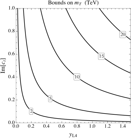
Figure 4: Bounds on the mass of the top partner derived from the recent ACME results. The bounds are derived by setting $f=800\;$GeV, although the dependence on $f$ is quite mild. The labels on the solid lines show the top partner mass $m_{T}$ in TeV.

Using the RGE Eq. (2.12), we obtain an electron EDM given by

$$\frac{d_{e}}{e}=-\frac{N_{c}}{64\pi^{4}}\frac{y_{e}}{\sqrt{2}}c_{T}\left[e^{2}Q_{u}^{2}+\frac{g^{2}}{4c_{\theta_{W}}^{2}}Q_{u}(T^{3}_{u}-Q_{u}s_{\theta_{W}}^{2})(1-4s_{\theta_{W}}^{2})+\frac{1}{2}g^{2}T^{3}_{u}Y_{Q}\right]\ln\frac{m_{T}^{2}}{m_{t}^{2}}\,.$$ (3.49)

The three terms in square brackets come from diagrams containing a virtual photon, a virtual $Z$-boson and a virtual $W$-boson respectively. Since, as we said, the $Z$-boson vector coupling to the electron is quite suppressed, the main contribution is coming from the photon loop, whereas the $W$-boson term gives a $\sim 40\%$ correction. In Eq. (3.49) the RG running of the EDM starts at $m_{T}$ and stops at the top mass. At that scale, indeed, we have to integrate the top, inducing an additional finite contribution to $C_{F\widetilde{F}}$ due to Eq. (3.47). Surprisingly, this contribution exactly cancels the one coming from top partners loops, Eq. (3.46), so that no net contribution to ${\cal O}_{F\widetilde{F}}$ is left below $m_{t}$.

In Fig. 4 we give the constraints on the mass of the $T$ top partner in the $(y_{L4},{\rm Im}[c_{t}])$ plane. To derive these bounds we assumed that the result in Eq. (3.49) provides the main correction to the electron EDM and no additional contributions (or at least no strong cancellations) are present. We can see that for natural values of the parameters of the theory, $y_{L4}\sim 1$ and ${\rm Im}[c_{t}]\sim 1$, the bounds from the electron EDM measurements can exclude top partner masses up to $\sim 15\;$TeV. This bound is significantly stronger than the current direct LHC exclusions and cannot be matched even in the high-luminosity LHC runs [40].

4 Conclusions

We performed a two-loop analysis of the EDM of the electron using the EFT approach. In particular, we calculated the RGEs of the dimension-6 CP-violating dipole operators at the two-loop order, as well as the one-loop RGEs of most relevant dimension-8 operators. We have shown that, due to selection rules, few operators can mix with EDM operators, as appreciated in Figure 1 where we present a summary of which and how dimension-6 operators enter into the EDM. We also commented on the RG running of the Wilson coefficients below the electroweak scale, and when CP-violating electron-nucleon interactions can be competitive with bounds on the electron EDM.

These results are important to provide a proper interpretation of the new ACME bound on the electron EDM in terms of constraints on BSM particles. The recent improvement on the bound allows to constrain TeV new-physics even when it only contributes at the two-loop level. We have shown this with some examples. In particular, we considered theories with leptoquarks or extra Higgs, obtaining bounds ranging $1-100$ TeV. We also considered two of the most motivated BSM scenarios for TeV new-physics, supersymmetry and composite Higgs. We first reinterpreted previous calculations in the EFT language. Then, we used our RGE two-loop results to understand which sectors or which new regions of the parameter space of these BSM are now constrained by the recent ACME result. In the MSSM case, for example, we showed how our two-loop results can provide new constraints on the small $\tan\beta$ region in the s-electron and wino sector. For the composite Higgs, after reinterpreting calculations on top-partners in the EFT language, we showed that bounds on these particles put them out of the reach of the LHC, unless they have CP-conserving couplings.

Therefore, we conclude that, unless we find a reason of why, contrary to the SM, the interactions in these BSM do respect CP, the ACME result makes these theories much less natural. More importantly, future improvement on the the electron EDM bound (see for example [42]) could constrain BSM beyond the reach of future colliders.

Appendix A EDM contributions from Barr–Zee diagrams

In this appendix we report the full expressions for the contributions to the electron EDM coming from CP-violating Higgs Yukawa’s originating from $H^{3}\bar{f}f$ operators.

Before giving the formulae for the EDM contributions, it is useful to introduce a few definitions. We define the $j(r,s)$ function as [25]

$$j(r,s)\equiv\frac{1}{r-s}\left(\frac{r\ln r}{r-1}-\frac{s\ln s}{s-1}\right)\,.$$ (A.1)

The Barr–Zee results with a CP-violating quark Yukawa can be rewritten in terms of the following integrals [43]

$$F_{1}(a,0) \equiv \int_{0}^{1}dx\frac{1}{x(1-x)}j\left(0,\frac{a}{x(1-x)}\right)$$ (A.2)

$$= \frac{2}{\sqrt{1-4a}}\left[{\rm Li}_{2}\left(1-\frac{1-\sqrt{1-4a}}{2a}\right)-{\rm Li}_{2}\left(1-\frac{1+\sqrt{1-4a}}{2a}\right)\right]\,,$$

and

$$F_{1}(a,b)\equiv\int_{0}^{1}dx\frac{1}{x(1-x)}j\left(b,\frac{a}{x(1-x)}\right)=\frac{1}{1-b}\left[F_{1}(a,0)-F_{1}(a/b,0)\right]\,.$$ (A.3)

Notice that the result in Eq. (A.3) follows immediately from the relation $j(r,s)=[j(0,s)-j(0,s/r)]/(1-r)$. For the diagrams involving a CP-violating electron Yukawa we need the following integrals

$$F_{2}(a,0)\equiv\int_{0}^{1}dx\frac{(1-x)^{2}+x^{2}}{x(1-x)}j\left(0,\frac{a}{x(1-x)}\right)=(1-2a)F_{1}(a,0)+2(\ln a+2)\,,$$ (A.4)

and

$$F_{2}(a,b) \equiv \int_{0}^{1}dx\frac{(1-x)^{2}+x^{2}}{x(1-x)}j\left(b,\frac{a}{x(1-x)}\right)$$ (A.5)

$$= \frac{1}{1-b}\left[(1-2a)F_{1}(a,0)-\left(1-2\frac{a}{b}\right)F_{1}\left(\frac{a}{b},0\right)+2\ln\frac{a}{b}\right]\,.$$

The expansion of the $F_{1}(a,0)$ integral for large $a$ is given by

$$F_{1}(a,0)\simeq\frac{1}{a}\left(2+\ln a\right)\,,$$ (A.6)

while for small $a$ one finds

$$F_{1}(a,0)\simeq\ln^{2}a+\frac{\pi^{2}}{3}\,.$$ (A.7)

We can now give the results for the Barr–Zee contributions to the electron EDM. The contribution from a ${\cal O}_{y_{f}}$ operator for a generic quark or a heavy lepton is given by

$$\frac{d_{e}}{e}=\frac{N_{c}}{64\pi^{4}}Q_{f}\frac{m_{f}m_{e}}{m_{h}^{2}}v\frac{{\rm Im}\,C_{y_{q}}}{\sqrt{2}\Lambda^{2}}\sum_{V=\gamma,Z}g_{e}^{V}g_{f}^{V}F_{1}\left(\frac{m_{f}^{2}}{m_{h}^{2}},\frac{m_{V}^{2}}{m_{h}^{2}}\right)\,,$$ (A.8)

where $g_{e,f}^{V}$ denote the vector couplings of the gauge boson $V$, namely $g_{f}^{\gamma}=eQ_{f}$ for the photon and $g_{f}^{Z}=g/(2c_{\theta_{W}})(T^{3}_{f}-2Q_{f}s_{\theta_{W}}^{2})$. The contribution from the ${\cal O}_{y_{e}}$ operator is instead

$$\frac{d_{e}}{e}=\frac{N_{c}}{64\pi^{4}}Q_{t}\frac{m_{t}^{2}}{m_{h}^{2}}v\frac{{\rm Im}\,C_{y_{e}}}{\sqrt{2}\Lambda^{2}}\sum_{V=\gamma,Z}g_{e}^{V}g_{t}^{V}F_{2}\left(\frac{m_{t}^{2}}{m_{h}^{2}},\frac{m_{V}^{2}}{m_{h}^{2}}\right)\,,$$ (A.9)

where we only included the contributions from top loops, since the ones from the other fermions are suppressed by the small Yukawa’s.

References

- [1] V. Andreev et al. [ACME Collaboration], Nature 562 (2018), 355.
- [2] B. Grzadkowski, M. Iskrzynski, M. Misiak and J. Rosiek, JHEP 1010 (2010) 085 [arXiv:1008.4884 [hep-ph]].
- [3] C. Cheung and C. H. Shen, Phys. Rev. Lett. 115 (2015) no.7, 071601 [arXiv:1505.01844 [hep-ph]].
- [4] J. Elias-Miró, J. R. Espinosa and A. Pomarol, Phys. Lett. B 747 (2015) 272 [arXiv:1412.7151 [hep-ph]].
- [5] R. Alonso, E. E. Jenkins and A. V. Manohar, Phys. Lett. B 739 (2014) 95 [arXiv:1409.0868 [hep-ph]].
- [6] E. E. Jenkins, A. V. Manohar and M. Trott, JHEP 1401 (2014) 035 [arXiv:1310.4838 [hep-ph]]. R. Alonso, E. E. Jenkins, A. V. Manohar and M. Trott, JHEP 1404 (2014) 159 [arXiv:1312.2014 [hep-ph]].
- [7] F. Boudjema, K. Hagiwara, C. Hamzaoui and K. Numata, Phys. Rev. D 43 (1991) 2223.
- [8] B. Gripaios and D. Sutherland, Phys. Rev. D 89 (2014) no.7, 076004 [arXiv:1309.7822 [hep-ph]].
- [9] J. Elias-Miró, J. R. Espinosa, E. Masso and A. Pomarol, JHEP 1308 (2013) 033 [arXiv:1302.5661 [hep-ph]].
- [10] S. Herrlich and U. Nierste, Nucl. Phys. B 455 (1995) 39 [arXiv:hep-ph/9412375].
- [11] A. Crivellin, S. Najjari and J. Rosiek, JHEP 1404 (2014) 167 [arXiv:1312.0634 [hep-ph]].
- [12] M. Frigerio, M. Nardecchia, J. Serra and L. Vecchi, JHEP 1810 (2018) 017 [arXiv:1807.04279 [hep-ph]].
- [13] M. Ciuchini, E. Franco, G. Martinelli, L. Reina and L. Silvestrini, Phys. Lett. B 316 (1993) 127 [arXiv:hep-ph/9307364].
- [14] S. M. Barr and A. Zee, Phys. Rev. Lett. 65 (1990) 21, Erratum: Phys. Rev. Lett. 65 (1990) 2920.
- [15] E. E. Jenkins, A. V. Manohar and P. Stoffer, JHEP 1801 (2018) 084 [arXiv:1711.05270 [hep-ph]].
- [16] P. Junnarkar and A. Walker-Loud, Phys. Rev. D 87 (2013) 114510 [arXiv:1301.1114 [hep-lat]].
- [17] D. Liu, A. Pomarol, R. Rattazzi and F. Riva, JHEP 1611 (2016) 141 [arXiv:1603.03064 [hep-ph]].
- [18] V. Cirigliano, W. Dekens, J. de Vries and E. Mereghetti, Phys. Rev. D 94 (2016) no.1, 016002 [arXiv:1603.03049 [hep-ph]]; Phys. Rev. D 94 (2016) no.3, 034031 [arXiv:1605.04311 [hep-ph]]. S. Alioli, V. Cirigliano, W. Dekens, J. de Vries and E. Mereghetti, JHEP 1705 (2017) 086 [arXiv:1703.04751 [hep-ph]]. J. A. Aguilar-Saavedra et al., arXiv:1802.07237 [hep-ph].
- [19] N. Yamanaka, B. K. Sahoo, N. Yoshinaga, T. Sato, K. Asahi and B. P. Das, Eur. Phys. J. A 53 (2017) no.3, 54 [arXiv:1703.01570 [hep-ph]]. K. Yanase, N. Yoshinaga, K. Higashiyama and N. Yamanaka, arXiv:1805.00419 [nucl-th].
- [20] I. Doršner, S. Fajfer, A. Greljo, J. F. Kamenik and N. Košnik, Phys. Rept. 641 (2016) 1 [arXiv:1603.04993 [hep-ph]].
- [21] W. Dekens, J. De Vries, M. Jung and K. K. Vos, arXiv:1809.09114 [hep-ph].
- [22] K. Fuyuto, M. Ramsey-Musolf and T. Shen, arXiv:1804.01137 [hep-ph].
- [23] L. Lavoura, Eur. Phys. J. C 29 (2003) 191 [arXiv:hep-ph/0302221].
- [24] C. Biggio, M. Bordone, L. Di Luzio and G. Ridolfi, JHEP 1610 (2016) 002 [arXiv:1607.07621 [hep-ph]].
- [25] Y. Nakai and M. Reece, JHEP 1708 (2017) 031 [arXiv:1612.08090 [hep-ph]].
- [26] C. Cesarotti, Q. Lu, Y. Nakai, A. Parikh and M. Reece, arXiv:1810.07736 [hep-ph].
- [27] Y. Kizukuri and N. Oshimo, Phys. Rev. D 46 (1992) 3025.
- [28] G. F. Giudice and A. Romanino, Phys. Lett. B 634 (2006) 307 [arXiv:hep-ph/0510197].
- [29] K. Agashe, R. Contino and A. Pomarol, Nucl. Phys. B 719 (2005) 165 [arXiv:hep-ph/0412089].
- [30] Y. Grossman and M. Neubert, Phys. Lett. B 474 (2000) 361 [arXiv:hep-ph/9912408]. T. Gherghetta and A. Pomarol, Nucl. Phys. B 586 (2000) 141 [arXiv:hep-ph/0003129]. S. J. Huber and Q. Shafi, Phys. Lett. B 498 (2001) 256 [arXiv:hep-ph/0010195]. S. J. Huber, Nucl. Phys. B 666 (2003) 269 [arXiv:hep-ph/0303183].
- [31] B. Keren-Zur, P. Lodone, M. Nardecchia, D. Pappadopulo, R. Rattazzi and L. Vecchi, Nucl. Phys. B 867 (2013) 394 [arXiv:1205.5803 [hep-ph]].
- [32] G. Panico and A. Wulzer, Lect. Notes Phys. 913 (2016) pp.1 [arXiv:1506.01961 [hep-ph]].
- [33] R. Barbieri, D. Buttazzo, F. Sala and D. M. Straub, JHEP 1207 (2012) 181 [arXiv:1203.4218 [hep-ph]]. M. Redi, Eur. Phys. J. C 72 (2012) 2030 [arXiv:1203.4220 [hep-ph]].
- [34] G. Panico and A. Pomarol, JHEP 1607 (2016) 097 [arXiv:1603.06609 [hep-ph]].
- [35] O. Matsedonskyi, G. Panico and A. Wulzer, JHEP 1301 (2013) 164 [arXiv:1204.6333 [hep-ph]]. D. Marzocca, M. Serone and J. Shu, JHEP 1208 (2012) 013 [arXiv:1205.0770 [hep-ph]]. A. Pomarol and F. Riva, JHEP 1208 (2012) 135 [arXiv:1205.6434 [hep-ph]].
- [36] G. Panico, M. Redi, A. Tesi and A. Wulzer, JHEP 1303 (2013) 051 [arXiv:1210.7114 [hep-ph]].
- [37] R. Contino, L. Da Rold and A. Pomarol, Phys. Rev. D 75 (2007) 055014 [arXiv:hep-ph/0612048].
- [38] G. Panico, M. Riembau and T. Vantalon, JHEP 1806 (2018) 056 [arXiv:1712.06337 [hep-ph]].
- [39] A. De Simone, O. Matsedonskyi, R. Rattazzi and A. Wulzer, JHEP 1304 (2013) 004 [arXiv:1211.5663 [hep-ph]].
- [40] O. Matsedonskyi, G. Panico and A. Wulzer, JHEP 1604 (2016) 003 [arXiv:1512.04356 [hep-ph]].
- [41] A. Czarnecki, W. J. Marciano and A. Vainshtein, Phys. Rev. D 67 (2003) 073006 Erratum: [Phys. Rev. D 73 (2006) 119901] [hep-ph/0212229].
- [42] W. B. Cairncross et al., Phys. Rev. Lett. 119 (2017) no.15, 153001 [arXiv:1704.07928 [physics.atom-ph]]. A. C. Vutha, M. Horbatsch and E. A. Hessels, Atoms 6, 3 (2018) [arXiv:1710.08785 [physics.atom-ph]]. Phys. Rev. A 98 (2018) no.3, 032513 [arXiv:1806.06774 [physics.atom-ph]].
- [43] J. Brod, U. Haisch and J. Zupan, JHEP 1311 (2013) 180 [arXiv:1310.1385 [hep-ph]].