Global Closed-form Approximation of Free Boundary for Optimal Investment Stopping Problems

Abstract

In this paper we study a utility maximization problem with both optimal control and optimal stopping in a finite time horizon. The value function can be characterized by a variational equation that involves a free boundary problem of a fully nonlinear partial differential equation. Using the dual control method, we derive the asymptotic properties of the dual value function and the associated dual free boundary for a class of utility functions, including power and non-HARA utilities. We construct a global closed-form approximation to the dual free boundary, which greatly reduces the computational cost. Using the duality relation, we find the approximate formulas for the optimal value function, trading strategy, and exercise boundary for the optimal investment stopping problem. Numerical examples show the approximation is robust, accurate and fast.

2010 MSC: 49L20, 90C46

Keywords: Optimal investment stopping problem, dual control method, free boundary, global closed-form approximation.

1 Introduction

There has been extensive research in utility maximization. Two main approaches are stochastic control (dynamic programming, HJB equation) and convex duality (static optimization, martingale representation). For excellent expositions of these two methods in utility maximization, see Fleming and Soner (1993), Karatzas and Shreve (1998), Pham (2009), and the references therein.

A variant of utility maximization of terminal wealth is that investors may stop the investment before or at the maturity to achieve the overall maximum of the expected utility, which naturally leads to a mixed optimal control and stopping problem. The early work on this line includes Karatzas and Wang (2000) and Dayanik and Karatzas (2003) for properties of the value function at the initial time, Ceci and Bassan (2004) for existence of viscosity solution of the variational equation, Henderson and Hobson (2008) for equivalence of the value function in the presence of a Markov chain process and power utility. None of the above papers discusses the free boundary problem. Jian et al. (2014) apply the dual transformation method to convert the nonlinear variational equation with power utility into an equivalent free boundary problem of a linear PDE and analyse qualitatively the properties of the free boundary and optimal strategies. The work is further extended in Guan et al. (2017) to a problem with a call option type terminal payoff and power utility.

It is well known that finding the free boundary of a variational equation is a difficult problem, see Peskir and Shiryaev (2006). One good example is American options pricing problem. The free boundary separates the exercise region from the continuation region and satisfies an integral equation which can be hardly solved, see Detemple (2005). Finding the free boundary is much more difficult for the optimal investment stopping problem than for the American options pricing problem as the former has a nonlinear PDE in the continuation region and a non-Lipschitz continuous utility function and may have one or more free boundaries whereas the latter has a linear PDE in the continuation region and a Lipschitz continuous payoff function and a unique free boundary. The dual transformation in Jian et al. (2014) and Guan et al. (2017) is a step in the right direction to simplify the primal nonlinear variational equation into the dual linear variational equation, however, finding the free boundary remains a challenging and open problem.

In this paper we study an optimal investment stopping problem for general utility functions with a requirement that the wealth is above a threshold value which could be a liability or the minimum living standard, called portfolio insurance. Using the dual transformation approach as in Jian et al. (2014) and Guan et al. (2017), we convert the primal variational equation into an equivalent free boundary problem of a linear PDE and show there exists a unique smooth free boundary that satisfies some integral equation for a class of utility functions, including power and non-HARA utilities, see Theorems 3.3 and 3.7. We then apply the asymptotic analysis to characterize the limiting behaviour of the free boundary as time to maturity tends to zero and to infinite, see Theorems 3.8 and 3.9. We construct a simple function that has the same property as the free boundary with matched limiting behaviour and use it as a global closed-form approximation to the free boundary, which is inspired by Xie et al. (2014) for a mortgage payment problem with a simple time-only, state-independent payoff and known initial value of the process, in contrast to our non-Lipschitz state-dependent payoff and unknown initial value of the dual process. Finally, using the duality relation, we recover the primal value function and the corresponding free boundary, see Theorem 3.11.

The main contribution of this paper is that we give a global closed-form approximation (GCA) to the free boundary of an optimal investment stopping problem for a class of general utility functions. There are several decisive benefits of the GCA: it provides a simple analytic formula for separating the stopping region and the continuation region, it gives the dual value function a semi closed-form integral representation which makes possible finding the optimal trading strategy in the continuation region, and it leads to fast and efficient computation. The key to this success is the explicit characterization of the asymptotic properties of the free boundary for the dual optimal stopping problem. To the best knowledge of the authors, this is the first time such results are reported in the literature for optimal investment stopping problems. Numerical tests show that GCA is accurate and fast, compared with the binomial tree method which itself is practical and efficient in solving optimal investment stopping problems, see Example 4.2.

The remaining of the paper is organized as follows. In Section 2, we introduce the optimal investment stopping problem, convert the HJB variational equation into an equivalent dual variational equation, show the existence and uniqueness of the dual solution and its properties, and establish the corresponding results for the original problem. In Section 3, we present the main results of this paper for a class of utilities which include power and non-HARA utilities, Theorem 3.7 shows the free boundary is monotone and smooth and satisfies an integral equation, Theorems 3.8 and 3.9 characterize the asymptotic behaviour of the free boundary when time to maturity is close to zero or infinite, Theorem 3.11 constructs a GCA to the free boundary. We also give two examples (Examples 3.4 and 3.6) to illustrate the fundamental difference of utility maximization with portfolio insurance and without. In Section 4, we perform some numerical tests to compare the results derived with the GCA and with the binomial tree method and show the suggested GCA is accurate, fast, and robust. In Section 5, we give the proofs of the main results. Section 6 concludes. The appendix provides the proof of Theorem 2.2 for the convenience of the reader.

2 Optimal Investment Stopping Problems

We consider a complete market equipped with a probability space $(\Omega,\mathscr{F},P)$ together with a natural filtration $(\mathscr{F}_{t})$ generated by a standard Brownian motion $W$, satisfying the usual conditions. It consists of one riskless savings account with interest rate $r>0$ and one risky asset satisfying the following stochastic differential equation (SDE)

$$dS_{t}=\mu S_{t}dt+\sigma S_{t}dW_{t},$$

where $\mu>0$ is the stock growth rate, and $\sigma>0$ is the stock volatility.

Let $(X_{t})_{0\leq t\leq T}$ denote the wealth process and $\pi_{t}$ the amount of wealth an investor holds in risky asset at time $t$. With continuous self-financing strategy, the wealth process $(X_{t})_{0\leq t\leq T}$ evolves as

$$dX_{t}=rX_{t}dt+\sigma\pi_{t}(\theta dt+dW_{t}),$$

where $\theta=\frac{\mu-r}{\sigma}$ is the market price of risk and $(\pi_{t})_{0\leq t\leq T}$ the portfolio process that is ${\cal F}_{t}$-progressively measurable and satisfies $E[\int^{T}_{0}|\pi_{t}|^{2}dt]<\infty$.

The optimal investment stopping problem is given by

$$\sup_{\pi,\tau}E\left[e^{-\beta\tau}U(X_{\tau}^{0,x,\pi}-K)\right],$$

where $U$ is a utility function, $\tau\in[0,T]$ is an $\mathscr{F}_{t}$-adapted stopping time, $\beta>0$ the utility discount factor, $K>0$ the minimum wealth threshold value. If $K=0$ then the problem is a standard utility maximization with investment and stopping. It turns out that $K>0$ and $K=0$ would lead to completely different optimal trading strategies for non-HARA utility, which indicates that one cannot simply change a portfolio insurance problem into a standard utility maximization by setting $K=0$ to get a seemingly simplified and equivalent problem, see Examples 3.4 and 3.6 for detailed discussions.

Assumption 2.1.

$U\in C^{2}$ is an increasing and strictly concave function on $[0,\infty)$, satisfying $U(0)=0$, $U(\infty)=\infty$, $U^{\prime}(0)=\infty$, $U^{\prime}(\infty)=0$, $U(x)<C(1+x^{p})$ for $x\geq 0$, where $C>0,\,0<p<1$ are constants, and $U(x)=-\infty$ for $x<0$.

Define the value function as

$$V(t,x)=\sup_{\tau,\pi}E\left[e^{-\beta(\tau-t)}U(X_{\tau}^{t,x,\pi}-K)|X_{t}=x\right]$$

for $(t,x)\in(0,T)\times(K,\infty)$. Then $V$ satisfies the following HJB variational equation (see Guan et al. (2017)):

$$\min\left\{-{\partial V\over\partial t}-\sup_{\pi}\mathscr{L}^{\pi}[V],V-U(x-K)\right\}=0$$ (2.1)

for $(t,x)\in(0,T)\times(K,\infty)$, where

$$\mathscr{L}^{\pi}[V]=rxV_{x}-\beta V+\pi(\mu-r)V_{x}+\frac{1}{2}\pi^{2}\sigma^{2}V_{xx},$$

$V_{x}$ denotes $\frac{\partial}{\partial x}V(t,x)$, $V$ and $V_{xx}$, are defined similarly. The boundary and terminal conditions are given by

$$V(t,K)=0,\ t\in(0,T),\quad V(T,x)=U(x-K),\ x\in(K,\infty).$$ (2.2)

Suppose that $V(t,\cdot)$ is strictly concave, then the maximum of $\mathscr{L}^{\pi}[V]$ is achieved at

$$\pi_{t}^{*}=-\frac{\theta}{\sigma}\frac{V_{x}}{V_{xx}},$$ (2.3)

and (2.1) is equivalent to

$$\min\left\{-{\partial V\over\partial t}+\frac{\theta^{2}}{2}\frac{V_{x}^{2}}{V_{xx}}-rxV_{x}+\beta V,\ V-U(x-K)\right\}=0$$ (2.4)

for $(t,x)\in(0,T)\times(K,\infty)$.

We use the dual method to solve the variational equation (2.4). The dual function of $U(\cdot-K)$ is defined by

$$\tilde{U}_{K}(y):=\sup_{x>K}\left[U(x-K)-xy\right]=\tilde{U}_{0}(y)-Ky,\quad y>0,$$

where $\tilde{U}_{0}$ is the dual function of $U$. It is easy to check that $\tilde{U}_{K}$ is continuously differentiable, decreasing, strictly convex, $\tilde{U}_{K}(0)=\infty$ and

$$-Ky\leq\tilde{U}_{K}(y)\leq\tilde{C}+\tilde{C}y^{\frac{p}{p-1}}-Ky,$$ (2.5)

where $\tilde{C}=\max\left\{C,(Cp)^{\frac{1}{p-1}}[p^{-1}-1]\right\}$.

Define the dual value function as

$$\tilde{V}(t,y)=\sup_{t\leq\tau\leq T}E\left[e^{-\beta(\tau-t)}\tilde{U}_{K}(Y_{\tau})|Y_{t}=y\right],$$

where $(Y_{t})_{0\leq t\leq T}$ is a dual process satisfying the SDE

$$dY_{t}=(\beta-r)Y_{t}dt-\theta Y_{t}dW_{t}.$$ (2.6)

Then the dual value function satisfies the following variational equation (see Guan et al. (2017)):

$$\min\left\{-{\partial\tilde{V}\over\partial t}-\frac{\theta^{2}}{2}y^{2}\tilde{V}_{yy}-(\beta-r)y\tilde{V}_{y}+\beta\tilde{V},\ \tilde{V}-\tilde{U}_{K}\right\}=0$$ (2.7)

for $(t,y)\in(0,T)\times(0,\infty)$, with the terminal condition given by

$$\tilde{V}(T,y)=\tilde{U}_{K}(y),\quad y\in(0,\infty).$$

Define

$$z=\log y,\ \tau=\frac{\theta^{2}}{2}(T-t),\ v(\tau,z)=\tilde{V}(t,y).$$

Then $v$ satisfies the following variational equation:

$$\min\left\{L[v],\ v-g\right\}=0$$ (2.8)

for $(\tau,z)\in\Omega_{T}:=(0,\theta^{2}T/2)\times\mathbb{R}^{1}$, with the initial condition given by $v(0,z)=g(z)$ for $z\in\mathbb{R}^{1}$, where

$$L[v]=v_{\tau}-v_{zz}+\kappa v_{z}+\rho v,\ \quad g(z)=\tilde{U}_{K}(e^{z}),$$ (2.9)

and constants $\nu,\rho,\kappa$ are defined by

$$\nu=\frac{2r}{\theta^{2}},\ \rho=\frac{2\beta}{\theta^{2}},\ \kappa=\nu-\rho+1.$$

The next result shows the existence of a unique solution of the variational equation (2.8) with monotonicity properties for each variable. Denote by $W^{1,2}_{p}(\Omega_{T})$ the Sobolev space and $W^{1,2}_{p,loc}(\Omega_{T})$ the local Sobolev space defined by $W^{1,2}_{p,loc}(\Omega_{T}):=\{v\in W^{1,2}_{p}(Q),\ \forall Q\subset\subset\Omega_{T}\}$.

Theorem 2.2.

Problem (2.8) has a unique solution $v\in C(\bar{\Omega}_{T})\cap W^{1,2}_{p,loc}(\Omega_{T})$ for $1<p<+\infty$, satisfying

$$g(z)\leq v(\tau,z)\leq\tilde{C}(e^{B\tau+\frac{p}{p-1}z}+1),\ (\tau,z)\in\Omega_{T},$$ (2.10)

where $B=|(\frac{p}{p-1})^{2}-\kappa\frac{p}{p-1}-\rho|+1$ and $\tilde{C}=\max\left\{C,(Cp)^{\frac{1}{p-1}}[1/p-1]\right\}$. Furthermore, $v$ satisfies

$$v_{z}\leq 0,\quad-v_{z}+v_{zz}>0,\quad v_{\tau}\geq 0,\quad(\tau,z)\in\Omega_{T}.$$ (2.11)

Proof.

See Appendix. ∎

Since $\tilde{V}(t,y)=v(\tau,z)$, using Theorem 2.2, we can easily derive the corresponding results for $\tilde{V}$.

Corollary 2.3.

Problem (2.7) has a unique solution $\tilde{V}\in C([0,T]\times(0,\infty))\cap W^{1,2}_{p,loc}([0,T)\times(0,\infty))$ for $1<p<+\infty$, satisfying

$$\tilde{U}_{K}(y)\leq\tilde{V}(t,y)\leq\tilde{C}(e^{B_{1}(T-t)}y^{{p\over p-1}}+1),\quad(t,y)\in[0,T)\times(0,\infty),$$

where $B_{1}=B\theta^{2}/2$ and $B,\,\tilde{C}$ are given in Theorem 2.2. Furthermore, $\tilde{V}$ is decreasing in $t$ and decreasing and strictly convex in $y$, satisfying

$$\lim_{y\rightarrow 0}-\tilde{V}_{y}(t,y)=+\infty,\ \lim_{y\rightarrow\infty}-\tilde{V}_{y}(t,y):=a\leq K,\ t\in(0,T).$$ (2.12)

Proof.

See Section 5. ∎

Remark 2.4.

We can easily find a strong solution $V$ to the variational HJB equation (2.4) with conditions (2.2) by defining

$$V(t,x)=\inf_{y>0}[\tilde{V}(t,y)+xy]$$ (2.13)

for $t\in(0,T)$ and $x\in(K,\infty)$, and $V$ is strictly increasing and strictly concave in $x$, see Jian et al. (2014) for details.

3 Main Results

In this section, we consider the dual utility function of the form

$$\tilde{U}_{K}(y)=\sum_{j=1}^{J}-\frac{1}{q_{j}}y^{q_{j}}-Ky,$$ (3.1)

where $q_{1}<q_{2}<\cdots<q_{J}<0$.

Example 3.1.

If $J=1$ and $q_{1}=\frac{\gamma}{\gamma-1}$ with $0<\gamma<1$, then $\tilde{U}_{0}(y)$ is the dual function of the power utility $U(x)=\frac{1}{\gamma}x^{\gamma}$. If $J=2$ and $q_{1}=-3,\ q_{2}=-1$, then $\tilde{U}_{0}(y)$ is the dual function of the non-HARA utility

$$U(x)=\frac{1}{3}H^{-3}(x)+H^{-1}(x)+xH(x),$$

where $H(x)=(\frac{2}{-1+\sqrt{1+4x}})^{1/2}$, see Bian and Zheng (2015).

Define $\phi:=L[g]$, where $L$ is defined in (2.9). Direct computation gives

$$\phi(z)=L[g](z)=\sum_{j=1}^{J}A_{j}e^{q_{j}z}-\nu Ke^{z},$$ (3.2)

where $A_{j}=q_{j}-\kappa-\rho/q_{j}$. Note that $A_{1}<A_{2}<\cdots<A_{J}$.

Define the continuation region in $z$-coordinate to be $\mathcal{C}_{z}:=\{(\tau,z);\,v(\tau,z)>g(z),\,0<\tau\leq\theta^{2}T/2\}$ and the exercise region to be $\mathcal{S}_{z}:=\{(\tau,z);\,v(\tau,z)=g(z),\,0<\tau\leq\theta^{2}T/2\}$. We need the following assumption for our main results.

Assumption 3.2.

The parameters of the model satisfy $K>0$ and $A_{1}>0$.

Now we can prove the existence of the free boundary.

Theorem 3.3.

Let Assumption 3.2 hold. Then there exists a unique free boundary $z(\tau)$ defined by

$$z(\tau):=\inf\{z;\,v(\tau,z)>g(z)\},\ 0<\tau\leq\theta^{2}T/2.$$ (3.3)

such that the continuation region $\mathcal{C}_{z}$ and the exercise region $\mathcal{S}_{z}$ can be written respectively as

$$\mathcal{C}_{z}=\left\{(\tau,z);\,z>z(\tau),\,0<\tau\leq\theta^{2}T/2\right\}$$ (3.4)

and

$$\mathcal{S}_{z}=\left\{(\tau,z);\,z\leq z(\tau),\,0<\tau\leq\theta^{2}T/2\right\}.$$ (3.5)

Proof.

See Section 5. ∎

Example 3.4.

In this example, we consider non-HARA utility ($J=2,\,q_{1}=-3,\,q_{2}=-1$ in (3.1)) for $K>0$. Since $A_{1}<A_{2}$, we discuss the following three cases.

• Case 1: $A_{1}\geq 0$. There exists a unique free boundary $z(\tau)$ defined by (3.3).

• Case 2: $A_{1}<0<A_{2}$ and $A_{2}^{2}+4A_{1}\nu K>0$. There exist two free boundaries $z_{1}(\tau)$ and $z_{2}(\tau)$ defined by

  $$z_{1}(\tau):=\inf\{z;\,v(\tau,z)=g(z)\},\ 0<\tau\leq\theta^{2}T/2,$$ (3.6)

  and

  $$z_{2}(\tau):=\sup\{z;\,v(\tau,z)=g(z)\},\ 0<\tau\leq\theta^{2}T/2,$$ (3.7)

  such that the continuation region and the exercise region are given by

  $$\mathcal{C}_{z}=\left\{(\tau,z);\,z<z_{1}(\tau)\ \hbox{or}\ z>z_{2}(\tau),\,0<\tau\leq\theta^{2}T/2\right\}$$ (3.8)

  and

  $$\mathcal{S}_{z}=\left\{(\tau,z);\,z_{1}(\tau)\leq z\leq z_{2}(\tau),\,0<\tau\leq\theta^{2}T/2\right\}.$$ (3.9)

  Moreover, $z_{1}(\tau)$ is increasing and $z_{2}(\tau)$ decreasing with limits

  $$\lim_{\tau\to 0}z_{1}(\tau)=-\frac{1}{2}\log\frac{-A_{2}-\sqrt{A_{2}^{2}+4A_{1}K\nu}}{2A_{1}},$$ (3.10)

  and

  $$\lim_{\tau\to 0}z_{2}(\tau)=-\frac{1}{2}\log\frac{-A_{2}+\sqrt{A_{2}^{2}+4A_{1}K\nu}}{2A_{1}}.$$ (3.11)

• Case 3: $A_{2}\leq 0$ or $A_{1}<0<A_{2}$ and $A_{2}^{2}+4A_{1}\nu K\leq 0$. There is no free boundary and it is not optimal to stop before the maturity.

Since the proof is slightly technical, we leave it in Section 5. Figure 1 (a) - (c) illustrates the three cases discussed above with $\mathcal{C}_{z}$ the continuation region and $\mathcal{S}_{z}$ the exercise region.

Remark 3.5.

For Example 3.4, simple algebra shows that $A_{i}=a_{i}\beta+b_{i}$, $i=1,2$, where $a_{1}=8/(3\theta^{2})$, $a_{2}=4/\theta^{2}$, $b_{1}=-2(2+r/\theta^{2})$, $b_{2}=-2(1+r/\theta^{2})$. Denote by

$$\beta_{1}:=-{b_{1}\over a_{1}}=\frac{3}{2}\theta^{2}+\frac{3}{4}r,\quad\beta_{2}:=-{b_{2}\over a_{2}}={1\over 2}\theta^{2}+{1\over 2}r.$$

Then $A_{1}\geq 0$ is equivalent to $\beta\geq\beta_{1}$ and $A_{2}\leq 0$ is equivalent to $\beta\leq\beta_{2}$. For the case $A_{1}<0<A_{2}$, or $\beta_{2}<\beta<\beta_{1}$, we need to check the sign of $A_{2}^{2}+4A_{1}\nu K$, which requires a more detailed but still simple analysis. Denote by

$$\beta_{3} := \beta_{2}+\sqrt{rK\left(\frac{4}{3}\theta^{2}+\frac{1}{3}r\right)+\frac{4}{9}r^{2}K^{2}}-\frac{2}{3}rK,$$

$$\beta_{4} := \beta_{2}-\sqrt{rK\left(\frac{4}{3}\theta^{2}+\frac{1}{3}r\right)+\frac{4}{9}r^{2}K^{2}}-\frac{2}{3}rK.$$

It is easy to check that $\beta_{4}<\beta_{2}<\beta_{3}<\beta_{1}$. It turns out that $A_{2}^{2}+4A_{1}\nu K\leq 0$ is equivalent to $\beta_{4}\leq\beta\leq\beta_{3}$. Combining the discussions above, we conclude that the parameter condition of Case 1 in Example 3.4 is equivalent to $\beta\geq\beta_{1}$, that of Case 2 to $\beta_{3}<\beta<\beta_{1}$, and that of Case 3 to $0<\beta\leq\beta_{3}$. Recall that $\beta$ is the utility discount factor. We see that when $\beta$ is small ($\beta\leq\beta_{3}$), there is no free boundary; when $\beta$ is in the middle ($\beta\in(\beta_{3},\beta_{1})$), there are two free boundaries; when $\beta$ is large ($\beta\geq\beta_{1}$), there is one free boundary. The threshold values $\beta_{3}$ and $\beta_{1}$ are critical in deciding different optimal trading strategies.

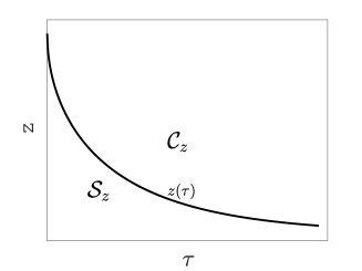
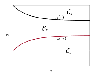
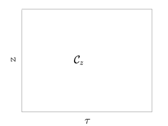
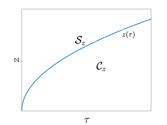
Figure 1: (a) $K>0$, $A_{1}\geq 0$;  (b) $K>0$, $A_{1}<0<A_{2},\,A_{2}^{2}+4A_{1}\nu K>0;$ (c) $K>0$, $A_{2}\leq 0\,\text{or}\,A_{1}<0<A_{2}$, $A_{2}^{2}+4A_{1}\nu K\leq 0$; (d) $K=0$, $A_{1}<0<A_{2}$.

The next example is to characterize the optimal exercise and continuation regions for the non-HARA utility discussed in Example 3.4 when the portfolio insurance value $K$ is set to be 0.

Example 3.6.

We assume $K=0$ and the same non-HARA utility as in Example 3.4. In this case we have $\beta_{3}=\beta_{2}$.

• Case 1: $A_{1}\geq 0$ (equivalently $\beta\geq\beta_{1}$). There is no free boundary and it is optimal to stop immediately.

• Case 2: $A_{1}<0<A_{2}$ (equivalently $\beta_{2}<\beta<\beta_{1}$). There exists a unique free boundary defined by

  $$z(\tau):=\inf\{z;v(\tau,z)=g(z)\},\ 0<\tau\leq\theta^{2}T/2.$$ (3.12)

  Moreover, $z(\tau)$ is increasing with limits

  $$\lim_{\tau\to 0}z(\tau)=\frac{1}{2}\log\Big{(}-\frac{A_{1}}{A_{2}}\Big{)},$$ (3.13)

  $$\lim_{\tau\to\infty}z(\tau)=\infty.$$ (3.14)

• Case 3: $A_{2}\leq 0$ (equivalently $\beta\leq\beta_{2}$). There is no free boundary and it is not optimal to stop before the maturity.

We leave the proof in Section 5. Figure 1 (d) illustrates the Case 2 discussed above with $\mathcal{C}_{z}$ the continuation region and $\mathcal{S}_{z}$ the exercise region.

Examples 3.4 and 3.6 show that there is a fundamental difference on optimal trading strategies with $K=0$ and $K>0$. For example, when $A_{1}<0<A_{2}$, there exists a unique free boundary for $K=0$ whereas there exist either two free boundaries or no free boundary for $K>0$, which implies that one has to use different optimal trading strategies in the presence of portfolio insurance $K>0$ and cannot simply set $K=0$ to reduce the problem into a standard utility maximization problem.

With Assumption 3.2, we can directly verify that $\phi(z)$ defined by (3.2) is strictly decreasing and there exists a unique $z_{0}\in\mathbb{R}$ such that

$$\phi(z_{0})=0.$$ (3.15)

Theorem 3.7.

Let Assumption 3.2 hold. Then the free boundary $z(\tau)$ defined by (3.3) is strictly decreasing with ${\displaystyle\lim_{\tau\rightarrow 0}}z(\tau)=z_{0}$, where $z_{0}$ is defined by (3.15), and $z(\tau)\in C[0,\theta^{2}T/2]\cap C^{\infty}(0,\theta^{2}T/2]$. Furthermore, $z(\tau)$ satisfies the following integral equation

$$-\int^{\infty}_{z_{0}}G(\tau,z(\tau)-y)\phi(y)dy+\int^{\tau}_{0}G(\tau-s,z(\tau)-z(s))\phi(z(s))z^{\prime}(s)ds=0,$$ (3.16)

where $G$ is the Green function defined by

$$G(\tau,z)=\frac{1}{\sqrt{4\pi\tau}}\exp\left(-\frac{(z-\kappa\tau)^{2}}{4\tau}-\rho\tau\right).$$ (3.17)

Proof.

See Section 5. ∎

In the following, we conduct the asymptotic analysis of the free boundary and construct the global approximation for the dual problem. We investigate the asymptotic behaviour of the free boundary near the expiry by using the integral equation (3.16).

Theorem 3.8.

Let Assumption 3.2 hold. Then the free boundary $z(\tau)$ defined by (3.3), for $0<\tau<<1$, satisfies approximately

$$z(\tau)\approx z_{0}-2A\sqrt{\tau},$$

where $A$ is a positive solution of the following equation

$$\frac{1}{2}e^{-A^{2}}-\frac{\sqrt{\pi}}{2}A+A^{2}\int_{0}^{1}e^{-A^{2}\eta^{2}}\frac{3\eta^{2}+\eta^{4}}{(1+\eta^{2})^{2}}d\eta=0.$$ (3.18)

The numerical solution of equation (3.18) is $A\approx 0.56292056798247$.

Proof.

See Section 5. ∎

The next result gives the asymptotic property of the free boundary $z(\tau)$ defined by (3.3) as time to maturity $\tau$ tends to infinite.

Theorem 3.9.

Let Assumption 3.2 hold and $z^{*}$ be the unique solution of the equation

$$\sum_{j=1}^{J}-\frac{1}{q_{j}}(q_{j}-\lambda)e^{(q_{j}-1)z}-K(1-\lambda)=0,$$

where $\lambda=\frac{1}{2}(\kappa-\sqrt{\kappa^{2}+4\rho})$. Then the free boundary defined by (3.3) satisfies

$$\lim_{\tau\rightarrow\infty}z(\tau)=z^{*}.$$

Proof.

See Section 5. ∎

Example 3.10.

Simple calculation shows that, for power utility ($J=1$ in (3.1)), we have

$$z_{0}=\frac{1}{q_{1}-1}\log\frac{K\nu}{A_{1}},\quad z^{*}=\frac{1}{q_{1}-1}\log\frac{Kq_{1}(1-\lambda)}{\lambda-q_{1}},$$

and, for non-HARA utility ($J=2,\,q_{1}=-3,\,q_{2}=-1$ in (3.1)), we have

$$\begin{split}z_{0}&=-\frac{1}{2}\log\frac{-A_{2}+\sqrt{A_{2}^{2}+4A_{1}\nu K}}{2A_{1}},\\ z^{*}&=-\frac{1}{2}\log\frac{-(q_{2}-\lambda)+\sqrt{(q_{2}-\lambda)^{2}+\frac{4}{3}(q_{1}-\lambda)(1-\lambda)}}{\frac{2}{3}(q_{1}-\lambda)}.\end{split}$$

By Assumption 3.2 and $q_{j}-\lambda>0,\,j=1,2$ (see (5.28)), we can verify that the expressions inside the above logarithmic functions are positive.

Now we seek a simple approximation formula for $z(\tau)$ defined by (3.3) such that (i) it has asymptotic expansion $z_{0}-2A\sqrt{\tau}$ for small $\tau$ and (ii) it approaches $z^{*}$ for large $\tau$. For this, we seek an approximation of the form

$$z_{*}(\tau):=z_{0}-2A\sqrt{\frac{1-e^{-b\tau}}{b}},$$

where $b>0$. To make it match with the large $\tau$ behaviour, we need $b=\frac{4A^{2}}{(z_{0}-z^{*})^{2}}$. Hence, the global closed-form approximation of the free boundary $z(\tau)$ defined by (3.3) is given by

$$z_{*}(\tau):=z_{0}-(z_{0}-z^{*})\sqrt{1-e^{-b^{*}\tau}},\ \ b^{*}=\frac{4A^{2}}{(z_{0}-z^{*})^{2}}.$$ (3.19)

The next result presents a global closed-form approximation of the free boundary for problem (2.4) with conditions (2.2).

Theorem 3.11.

Let the dual utility function be given by (3.1) and Assumption 3.2 hold. Let $z_{*}(\tau)$ in (3.19) be the global closed form approximation (GCA) to the free boundary $z(\tau)$ defined by (3.3). Then the unique free boundary of problem (2.4) with condition (2.2) is strictly decreasing and approximately determined by

$$x(t)=-\tilde{U}_{K}^{\prime}\left(\exp\left(z_{*}(\theta^{2}(T-t)/2)\right)\right),\ 0\leq t\leq T.$$

Furthermore, the primal value function is given by

$$V(t,x)=\tilde{V}(t,I(t,x))+xI(t,x),$$

and the optimal feedback control is given by

$$\pi^{*}_{t}=\frac{\theta}{\sigma}I(t,x)\tilde{V}_{yy}(t,I(t,x)),$$ (3.20)

where $\tilde{V}$ is the dual value function, approximately given by

$$\tilde{V}(t,y)=\tilde{U}_{K}(y)-\int_{0}^{\tau}\int_{z_{*}(s)}^{\infty}G\left(\tau-s,\ln y-w\right)\phi(w)dwds,$$ (3.21)

$\tau=\theta^{2}(T-t)/2$, and $y=I(t,x)$ is the unique solution of the equation $\tilde{V}_{y}(t,y)+x=0$ for $x>K$.

Proof.

See Section 5. ∎

Remark 3.12.

In the continuation region, the optimal feedback control $\pi^{*}$ can be computed either with (2.3) using the primal value function or with (3.20) using the dual value function. The two methods would produce the same optimal trading strategy due to the strong duality relation. It is in general more difficult to find the primal value function than to find the dual value function as the former satisfies a nonlinear PDE in the continuation region whereas the latter a linear PDE. The dual value function has an integral representation which makes possible computing the optimal control, provided the dual free boundary is known. This is where the GCA plays a pivotal role. It would be virtually impossible without the GCA to determine the optimal control in the continuation region as both the primal and dual value functions depend on unknown free boundaries.

4 Numerical Examples

In this section, we compare the numerical results derived using the global closed-form approximation (GCA) and the binomial tree method (BTM). We now briefly explain to use BTM to solve our problem. BTM cannot be directly applied to solve the original investment stopping problem, however, it can be used to solve the dual optimal stopping problem which is essentially an American options pricing problem with one additional difficulty, that is, one has to find the initial value $y$ of the dual process from the equation $\tilde{V}_{y}(t,y)+x=0$ while $\tilde{V}$ is to be determined. To circumvent the problem, we use the following procedure.

First, we fix an arbitrary $y_{0}>0$ and build a binomial tree for the dual process $Y$ up to time $T$ and then use the dynamic programming method to solve the dual optimal stopping problem and find the value $\tilde{V}_{y}(0,y_{0})$ at time 0. We then check the sign of $\tilde{V}_{y}(0,y_{0})+x$: if positive, we decrease the value of $\tilde{V}_{y}(0,y_{0})$ by setting $y_{1}=y_{0}/10$; if negative, we increase the value of $\tilde{V}_{y}(0,y_{0})$ by setting $y_{1}=10y_{0}$. Repeat the process and get $\tilde{V}_{y}(0,y_{1})$. If $\tilde{V}_{y}(0,y_{1})+x$ and $\tilde{V}_{y}(0,y_{0})+x$ have the same sign, we set $y_{0}=y_{1}$ and repeat the process above; if they have different signs, we have found an interval, bounded by $y_{0}$ and $y_{1}$, that contains a solution to the equation $V_{y}(t,y)+x=0$. We then use the bisection method to find $y$ with linear convergence. Once the initial value $y$ for the dual process is determined, we can get easily the value $\tilde{V}(0,y)$ and the free boundary for the dual problem. Finally, using the dual relation, we can find the optimal value and the free boundary for the primal problem.

Example 4.1.

We discuss the free boundary and the optimal strategy of the optimal investment stopping problem (2.4) with conditions (2.2) for power utility and non-HARA utility defined in Example 3.1.

The parameters used are $\mu=0.1$, $\beta=0.1$, $r=0.05$, $\sigma=0.3$, $K=1$, $\gamma=0.5$, $T=1$. The number of time steps for binomial tree method is $N=700$, which gives $4$ decimal point accuracy. These parameters satisfy Assumption 3.2.

In Figure 2 we plot the optimal exercise boundaries for power and non-HARA utilities using both the global closed-form approximation (GCA) and the binomial tree method (BTM). It is clear that the GCA and the BTM produce the free boundaries with the same shape and very small gaps. In Figure 3 we depict the sample paths of the optimal wealth and the corresponding optimal trading strategy using the GCA for power and non-HARA utilities. We can see that the optimal trading strategy becomes zero after time $\tau_{0}$, the first time the optimal wealth process hits the free boundary before the terminal time $T$, and $\tau_{0}$ is the optimal stopping time of investing in risky assets and the optimal wealth becomes $X_{t}=X_{\tau_{0}}e^{r(t-\tau_{0})}$ for $\tau_{0}\leq t\leq T$.

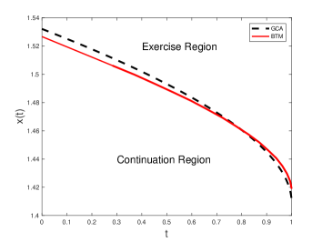
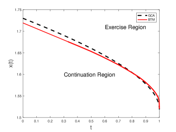
Figure 2: (a) The optimal exercise boundary compared with BTM for power utility;  (b) The optimal exercise boundary compared with BTM for non-HARA utility.

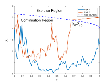
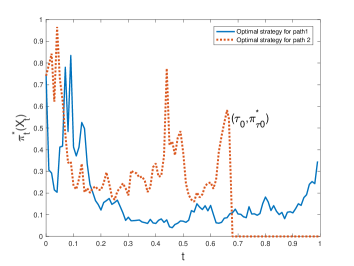
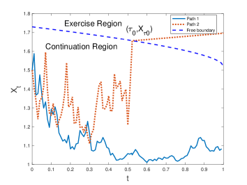
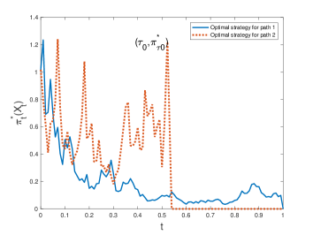
Figure 3: (a) Two different sample paths of wealth with initial wealth $x_{0}=1.4$ and optimal strategy for power utility. (b) Two different sample paths of wealth with initial wealth $x_{0}=1.5$ and optimal strategy for non-HARA utility.

Example 4.2.

In this example, we compare the optimal values and the optimal strategies obtained by the closed-form approximation and the binomial tree method at the initial time.

• For power and non-HARA utility, we compare the numerical results between GCA and BTM. The parameters used are $\mu=0.1$, $\beta=0.1$, $r=0.05$, $\sigma=0.3$, $K=1$, $\gamma=0.5$, $T=1$, $t=0,$ initial wealth $x_{0}=1.5$, number of time steps for binomial tree approach $N=700$. The numerical result is shown in Table LABEL:table-1.

• In Table LABEL:table-2, we give the mean and standard deviation of the absolute and relative difference between BTM and GCA for power and non-HARA utility. We fix $K=1$, $T=1$, $t=0,$ initial wealth $x_{0}=1.5$, and number of time steps for binomial tree approach $N=700$. The rest parameters are selected randomly: $10$ samples of $\mu$ from the uniform distribution on interval $[0.05,0.15]$, $r$ on $[0.02,0.08]$, $\beta$ on $[0.05,0.15]$, $\sigma$ on $[0.10,0.40]$, $\gamma$ on $[0.2,0.6]$. We also require the parameters satisfy Assumption 3.2.

From the numerics in Table LABEL:table-2, we observe that the difference between the GCA and BTM optimal values is very small, whereas the computational time for GCA is much less than that for BTM. The GCA is shown to be correct and fast. Compared to the optimal values, the error for computing the optimal strategies using both the BTM and GCA is bigger. This is not surprising, as the optimal strategies are computed with the derivatives of the value functions.

Table 1: Comparison between GCA and BTM for Example 4.2 (i).

	Power utility		Non-HARA utility
	Optimal value	Optimal strategy	Optimal value	Optimal strategy
GCA value	1.4128	0.6558	1.5094	0.6776
BTM value	1.4031	0.7454	1.5116	0.6846
Difference	0.0096	0.0899	0.0022	0.0069
Relative difference	0.0069	0.1206	0.0015	0.0101
Time for GCA	22.7s	10.9s	11.4s	5.6s
Time for BTM	1683.2s	1664.2s	2777.6s	2744.6s

Table 2: Comparison between GCA and BTM for Example 4.2 (ii).

	Power utility		Non-HARA utility
	Optimal value	Optimal strategy	Optimal value	Optimal strategy
Avg difference	0.0074	0.0969	0.0034	0.0281
Std difference	0.0050	0.1495	0.0062	0.0462
Avg relative difference	0.0050	0.0745	0.0022	0.0630
Std relative difference	0.0033	0.1145	0.0045	0.0919
Avg time for GCA	23.2s	8.2s	23.0s	9.3s
Avg time for BTM	2640.9s	2609.6s	2878.6s	2844.2s

5 Proofs

In this section we give detailed proofs of the results of the paper.

5.1 Proof of Corollary 2.3

Proof.

Everything is a straightforward translation of Theorem 2.2. We only need to show (2.12) holds. For some fixed $y_{0}>0$ and $y<y_{0}$, using $\tilde{U}_{K}(0)=\infty$ and the convexity of $\tilde{V}$ in $y$, we have

$$\tilde{V}_{y}(t,y)\leq\frac{\tilde{V}(t,y_{0})-\tilde{V}(t,y)}{y_{0}-y}\leq\frac{\tilde{V}(t,y_{0})-\tilde{U}_{K}(y)}{y_{0}-y},$$

which gives ${\displaystyle\lim_{y\rightarrow 0}}\left(-\tilde{V}_{y}(t,y)\right)=+\infty$. Similarly, for some fixed $y_{0}>0$ and $y_{0}<y$, using (2.5), we obtain

$$0\leq-\tilde{V}_{y}(t,y)\leq-\frac{\tilde{V}(t,y)-\tilde{V}(t,y_{0})}{y-y_{0}}\leq-\frac{\tilde{U}_{K}(y)-\tilde{V}(t,y_{0})}{y-y_{0}}\leq-\frac{-Ky-\tilde{V}(t,y_{0})}{y-y_{0}},$$

which gives ${\displaystyle\lim_{y\rightarrow\infty}}\left(-\tilde{V}_{y}(t,y)\right):=a\leq K$. ∎

5.2 Proof of Theorem 3.3

Proof.

In the exercise region, we immediately have $v_{z}=g_{z}$. In the continuation region, since $v_{z}(0,z)=g_{z}$ and $v_{z}(\tau,z)=g_{z}$ for $(\tau,z)\in\partial\mathcal{C}_{z}$, and by Assumption 3.2 and $q_{j}<0$, we have

$$L[g_{z}]=\phi^{\prime}(z)=\sum_{j=1}^{J}A_{j}q_{j}e^{q_{j}z}-K\nu e^{z}\leq 0.$$

On the other hand, in the continuation region it holds that $L[v_{z}]=0$. So we have $L[v_{z}-g_{z}]\geq 0$ in the continuation region. By comparison, we obtain that

$$v_{z}-g_{z}\geq 0.$$

As a consequence, if $(\tau,z_{1})\in\mathcal{C}_{z}$, i.e., $v(\tau,z_{1})>g(z_{1})$, then for any $z_{2}>z_{1}$,

$$v(\tau,z_{2})-g(z_{2})\geq v(\tau,z_{1})-g(z_{1})>0,$$

from which we infer that $(\tau,z_{2})\in\mathcal{C}_{z}$. This indicates each $\tau$-section of $\mathcal{C}_{z}$ is connected. The existence of the free boundary $z(\tau)$ now follows. We obtain (3.3) and (3.4). Moreover, (3.5) follows from (3.4). ∎

5.3 Proof of Example 3.4

Proof.

Case 1: If $A_{1}>0$, from Theorem 3.3, we know there exists a unique free boundary $z(\tau)$ defined by (3.3). If $A_{1}=0,$ then $A_{2}>A_{1}=0,$ Theorem 3.3 implies that there exists a unique free boundary $z(\tau)$ defined by (3.3).

Case 2: We now prove (3.6) - (3.9). Denote that $\Lambda:=\{(\tau,z);\,z_{1}(\tau)\leq z\leq z_{2}(\tau),\,0<\tau\leq\theta^{2}T/2\}$. Since $A_{1}<0<A_{2},$ $A_{2}^{2}+4A_{1}\nu K>0$ and $\phi(z)=e^{z}(A_{1}e^{-4z}+A_{2}e^{-2z}-\nu K)$, then there exists two roots for equation $\phi(z)=0$. We denote the two roots by $z_{I},\ z_{II}$ with $z_{I}<z_{II}$. By a direct computation, we have

$$z_{I}=-\frac{1}{2}\log\frac{-A_{2}-\sqrt{A_{2}^{2}+4A_{1}K\nu}}{2A_{1}},$$

$$z_{II}=-\frac{1}{2}\log\frac{-A_{2}+\sqrt{A_{2}^{2}+4A_{1}K\nu}}{2A_{1}}.$$

Then from the definition of the exercise region $\mathcal{S}_{z}=\{(\tau,z);\,v(\tau,z)=g(z),\,0<\tau\leq\theta^{2}T/2\}$ and the variational equation (2.8) , we have $L[v]=L[g]=\phi(z)\geq 0$ for $(\tau,z)\in\mathcal{S}_{z}.$ This implies that

$$\mathcal{S}_{z}\subseteq\left\{(\tau,z);\,\phi(z)\geq 0,\,0<\tau\leq\theta^{2}T/2\right\}=\left\{0<\tau\leq\theta^{2}T/2,\ z_{I}\leq z\leq z_{II}\right\}.$$

This shows that the $\tau$-section $\{z;\,v(\tau,z)=g(z),\,0<\tau\leq\theta^{2}T/2\}$ of the exercise region $\mathcal{S}_{z}$ is bounded. Therefore, $z_{1}(\tau)$ and $z_{2}(\tau)$ in (3.6) - (3.7) are well defined. By the definitions of $z_{1}(\tau)$ and $z_{2}(\tau)$, we obtain that $\mathcal{S}_{z}\subseteq\Lambda$. Now, we prove that

$$\Lambda\subseteq\mathcal{S}_{z}.$$ (5.1)

Since

$$\left\{(\tau,z);\,z=z_{1}(\tau)\,or\,z=z_{2}(\tau),\,0<\tau\leq\theta^{2}T/2\right\}\subseteq\mathcal{S}_{z}\subseteq\left\{(\tau,z);\,\phi(z)\geq 0,\,0<\tau\leq\theta^{2}T/2\right\},$$

we have $\Lambda\subseteq\left\{(\tau,z);\,\phi(z)\geq 0,\,0<\tau\leq\theta^{2}T/2\right\}$. Assume that (5.1) is false. Then there exists a non-empty subset $\mathscr{N}=\mathcal{C}_{z}\cap\Lambda$ and the parabolic boundary $\partial_{p}\mathscr{N}\subseteq\bar{\Omega}_{T}-\mathcal{C}_{z}$. Here $\bar{\Omega}_{T}$ denotes the closure of $\Omega_{T}$. Thus

$$L[v]=0,\ (\tau,z)\in\mathscr{N},$$

$$L[g]=\phi(z)\geq 0,\ (\tau,z)\in\mathscr{N},$$

$$v=g,\ (\tau,z)\in\partial_{p}\mathscr{N}.$$

By the comparison principle, $v\leq g$ in $\mathscr{N}$, which implies that $\mathscr{N}=\emptyset$. Hence the contradiction arises. Therefore, (5.1) holds. So $\Lambda=\mathcal{S}_{z}$, i.e., (3.9) holds true. (3.8) follows from (3.9).

Next, we prove the monotonicity of the two free boundaries. If $z_{1}(\tau)$ is not increasing, there exist $\tau_{1}<\tau_{2}$ such that $z_{1}(\tau_{1})>z_{1}(\tau_{2})$. Since $v_{\tau}\geq 0$ (see (2.11)), we have

$$g(z_{1}(\tau_{2}))=v(\tau_{2},z_{1}(\tau_{2}))\geq v(\tau_{1},z_{1}(\tau_{2}))>g(z_{1}(\tau_{2})),$$

which is a contradiction. Hence, $z_{1}(\tau)$ is increasing. Similarly, $z_{2}(\tau)$ is decreasing.

Finally, we prove (3.10) and (3.11). If

$$\lim_{\tau\to 0}z_{1}(\tau)>z_{I},$$

then for any $z$ satisfying

$$\lim_{\tau\to 0}z_{1}(\tau)>z>z_{I},$$

and $\tau=0$, we have

$$0 = v_{\tau}-v_{zz}+\kappa v_{z}+\rho v$$

$$= v_{\tau}+\phi(z)>0,$$

where the last inequality follows from the fact that $v_{\tau}\geq 0$ and $\phi(z)>0$ for $z_{I}<z<z_{II}$. This is a contradiction. Hence, (3.10) holds. By a similar argument, we can obtain (3.11).

Case 3: In fact, if $A_{2}\leq 0$ or $A_{1}<0<A_{2}$, $A_{2}^{2}+4A_{1}\nu K\leq 0$, then $L[g]=\phi(z)=e^{z}(A_{1}e^{-4z}+A_{2}e^{-2z}-\nu K)\leq 0$. Hence, $g$ is a subsolution of problem

$$L[v]=0,\ (\tau,z)\in\Omega_{T},$$ (5.2)

$$v(0,z)=g(z),\ z\in\mathbb{R}^{1}.$$ (5.3)

Denote the solution of the problem (5.2) - (5.3) by $\tilde{v}$. Then by comparison, we obtain that

$$\tilde{v}-g\geq 0\ \text{in}\ \Omega_{T}.$$

Therefore, $\tilde{v}$ is also the solution of problem (2.8). ∎

5.4 Proof of Example 3.6

Proof.

Case 1 and Case 3 can be easily proved as follows: Since $K=0$, we have $L[g]=\phi(z)=A_{1}e^{-3z}+A_{2}e^{-z}\geq 0$ if $A_{1}\geq 0$ or $\phi(z)\leq 0$ if $A_{2}\leq 0$ due to the relation $A_{1}<A_{2}$. If $\phi(z)\leq 0$, then by the same argument as in the proof of Example 3.4, we conclude that there is no free boundary and it is not optimal to stop before the maturity. If $\phi(z)\geq 0$, then $v=g$ is the solution to problem (2.8), which implies that there is no free boundary and it is optimal to stop immediately.

Next we prove Case 2. We can show (3.12), (3.13) and monotonicity of $z(\tau)$ following a similar argument as in the proof of Example 3.4. We only need to prove (3.14). If $z(\tau)$ is bounded, then we have $\displaystyle{\lim_{\tau\to\infty}}z(\tau)<\infty$. Denote $\displaystyle{\lim_{\tau\to\infty}}z(\tau):=a$.

We rewrite problem (2.8) as

$$L[v]=I_{\{z\geq z(\tau)\}}\phi(z),\ (\tau,z)\in\Omega_{T},$$

$$v(0,z)=g(z),\ z\in\mathbb{R},$$

where $I_{A}$ is the indicator function of set $A$. By Green’s identity, we have

$$v(\tau,z)=\int_{-\infty}^{\infty}G(\tau,z-y)g(y)dy+\int_{0}^{\tau}\int^{\infty}_{z(\tau-s)}G(s,z-y)\phi(y)dyds,$$

where $G$ is the Green function defined by (3.17). We set

$$\Lambda_{1}(\tau)=\frac{1}{3}e^{-3z(\tau)-3A_{1}\tau}+e^{-z(\tau)-A_{2}\tau},$$

$$\Lambda_{2}(\tau)=\frac{A_{1}}{\sqrt{\pi}}e^{-3z(\tau)}\int_{0}^{\tau}e^{-3A_{1}s}\int_{\frac{z(\tau-s)-z(\tau)+(\kappa+6)s}{2\sqrt{s}}}^{\infty}e^{-\eta^{2}}d\eta ds,$$

$$\Lambda_{3}(\tau)=\frac{A_{2}}{\sqrt{\pi}}e^{-z(\tau)}\int_{0}^{\tau}e^{-A_{2}s}\int_{\frac{z(\tau-s)-z(\tau)+(\kappa+2)s}{2\sqrt{s}}}^{\infty}e^{-\eta^{2}}d\eta ds.$$

Since $v(\tau,z(\tau))=g(z(\tau))$, we have

$$\Lambda_{1}(\tau)+\Lambda_{2}(\tau)+\Lambda_{3}(\tau)=g(z(\tau)).$$

By dominated convergence theorem, we have

$$\lim_{\tau\to\infty}\Lambda_{2}(\tau) = \frac{A_{1}}{\sqrt{\pi}}e^{-3a}\int_{0}^{\infty}e^{-3A_{1}s}\int_{\frac{(\kappa+6)\sqrt{s}}{2}}^{\infty}e^{-\eta^{2}}d\eta ds,$$

$$= -\frac{\kappa+6}{6\sqrt{\pi}}e^{-3a}\int_{0}^{\infty}e^{-(\frac{\kappa^{2}}{4}+\rho)t^{2}}dt<\infty.$$

Since $A_{1}<0<A_{2}$, we have

$$\lim_{\tau\to\infty}\Lambda_{3}(\tau)\leq A_{2}e^{-a}\int_{0}^{\infty}e^{-A_{2}s}ds<\infty,$$

$$\lim_{\tau\to\infty}\Lambda_{1}(\tau)=\infty.$$

As $\displaystyle{\lim_{\tau\to\infty}}g(z(\tau))=g(a)<\infty$, this leads to a contradiction. Hence, we obtain that $z(\tau)$ is increasing and unbounded, i.e., (3.14) holds. ∎

5.5 Proof of Theorem 3.7

Proof.

From Theorem 3.3, the variational problem (2.8) can be written as

$$L[v]=0\ \text{for}\ z>z(\tau),\ 0<\tau\leq\theta^{2}T/2,$$ (5.4)

$$v(\tau,z)=g(z)\ \text{for}\ z\leq z(\tau),\ 0<\tau\leq\theta^{2}T/2,$$ (5.5)

$$v_{z}(\tau,z(\tau))=g_{z}(z(\tau)),\ 0<\tau\leq\theta^{2}T/2,$$ (5.6)

$$v(0,z)=g(z),\ z\in\mathbb{R},$$

where $L$ and $g$ is defined as in (2.9).

Firstly, we claim that $z(\tau)$ is non-increasing. Otherwise, there exists some $0<\tau_{0}<\tau_{1}$ such that $z(\tau_{0})<z(\tau_{1})$. Then since $v_{\tau}\geq 0$ (see (2.11)), we obtain that

$$0=v(\tau_{1},z(\tau_{1}))-g(z(\tau_{1}))\geq v(\tau_{0},z(\tau_{1}))-g(z(\tau_{1}))>0,$$

where the second inequality follows from the definition of the free boundary $z(\tau)$. This leads to contradiction. Then we claim that

$$z(\tau)<z_{0}\ \text{for}\ \tau>0.$$ (5.7)

Let $\bar{v}=v-g$. We rewrite the variational problem (2.8) as

$$\min\{L[\bar{v}]+\phi(z),\ \bar{v}\}=0,\ (\tau,z)\in\Omega_{T},$$ (5.8)

$$\bar{v}(0,z)=0,\ z\in\mathbb{R},$$ (5.9)

where $\phi(z)$ is defined by (3.2).

Let $U$ be the solution to

$$L[U]=-\phi(z),\ (\tau,z)\in\Omega:=\{(\tau,z)\in\Omega_{T};\,z>z_{0}\},$$ (5.10)

$$U(\tau,z)=0,\ (\tau,z)\in\partial_{p}\Omega,$$ (5.11)

where $\partial_{p}\Omega$ is the parabolic boundary of $\Omega$.

Since $\phi(z)$ is strictly decreasing and $z>z_{0}$, by (3.15), we have $L[U]=-\phi(z)>0$ in $\Omega$. By the maximum principle (see (Lieberman, 1996, Theorem 2.7)), we have $U>0$ in $\Omega$. Then Hopf’s lemma (see (Lieberman, 1996, Lemma 2.8)) leads to $U_{z}(\tau,z_{0})>0$ for $\tau>0$. By (5.8) - (5.11), we have $L[\bar{v}]\geq-\phi(z)=L[U]$ and $\bar{v}(\tau,z)\geq 0=U(\tau,z)$ for $(\tau,z)\in\partial_{p}\Omega$. By the comparison principle (Lieberman, 1996, Corollary 2.5), we see that $\bar{v}\geq U>0$ in $\Omega$. This implies that $z(\tau)\leq z_{0}$. Otherwise, there exists some $z_{1}\in(z_{0},z(\tau))$ such that $\bar{v}(\tau,z_{1})=0$.

If there exists some $\tau_{0}>0$ such that $z(\tau_{0})=z_{0}$, then we have

$$\bar{v}(\tau_{0},z(\tau_{0}))=U(\tau_{0},z(\tau_{0}))=0.$$

Hopf’s lemma (see (Lieberman, 1996, Lemma 2.8)) implies that

$$\bar{v}_{z}(\tau_{0},z(\tau_{0}))>U_{z}(\tau_{0},z(\tau_{0}))>0.$$

Since $\bar{v}_{z}(\tau,z(\tau))=0$, for any $\tau>0$, this leads to contradiction. So (5.7) is proved.

Hence, we have ${\displaystyle\lim_{\tau\rightarrow 0}}z(\tau)\leq z_{0}$. If ${\displaystyle\lim_{\tau\rightarrow 0}}z(\tau)<z_{0}$, then for some $z\in({\displaystyle\lim_{\tau\rightarrow 0}z(\tau),z_{0})}$, by (5.4), we have

$$L[v]|_{\tau=0}=[v_{\tau}-v_{zz}+\kappa v_{z}+\rho v]|_{\tau=0}=0.$$

This leads to

$$v_{\tau}|_{\tau=0}=[v_{zz}-\kappa v_{z}-\rho v]|_{\tau=0}=-\phi(z)<0,$$

where the last inequality follows from $\phi$ is strictly decreasing, $\phi(z_{0})=0$ and $z<z_{0}$. This contradicts with the fact that $v_{\tau}(0,z)\geq 0$ (see (2.11))

We now prove that $z(\tau)\in C[0,\theta^{2}T/2]$. If this is not true, then there exists some $\tau_{0}\in[0,\theta^{2}T/2)$ such that

$$z_{1}<z_{2},\ \text{where}\ z_{1}=\lim_{\tau\rightarrow\tau_{0}^{+}}z(\tau),\ z_{2}=\lim_{\tau\rightarrow\tau_{0}^{-}}z(\tau).$$

By (5.7), we have $z_{1},\ z_{2}\leq z_{0}$. For any $z\in[z_{1},z_{2}]$, by (5.4), we have

$$L[v]|_{\tau=\tau_{0}}=[v_{\tau}-v_{zz}+\kappa v_{z}+\rho v]|_{\tau=\tau_{0}}=0.$$

For any $z\in[z_{1},z_{2}]$, this leads to

$$v_{\tau}|_{\tau=\tau_{0}}=[v_{zz}-\kappa v_{z}-\rho v]|_{\tau=\tau_{0}}=-\phi(z)\leq 0,$$

where the last inequality follows from $\phi$ is decreasing, $\phi(z_{0})=0$ and $z_{1},\,z_{2}\leq z_{0}$. By (2.11), this means $\phi(z)=0$ for any $z\in[z_{1},z_{2}]$, while $\phi$ is a strictly decreasing function. The contradiction arises. Therefore $z(\tau)\in C[0,\theta^{2}T/2]$ is true. Furthermore we can use the bootstrap argument developed by Friedman (1975) to conclude that $z(\tau)\in C^{\infty}(0,\theta^{2}T/2]$.

To prove the rest of the results in this theorem, by (5.5), we have

$$v(\tau,z(\tau))=g(z(\tau)),\ \tau>0.$$ (5.12)

Differentiating (5.12) in $\tau$, by (5.6), we obtain

$$v_{\tau}(\tau,z(\tau))=0.$$ (5.13)

Furthermore, (5.4) implies

$$L[v](\tau,z(\tau))=v_{\tau}(\tau,z(\tau))-v_{zz}(\tau,z(\tau))+\kappa v_{z}(\tau,z(\tau))+\rho v(\tau,z(\tau))=0,$$

which leads to

$$\begin{split}v_{zz}(\tau,z(\tau))&=\kappa g_{z}(z(\tau))+\rho g(z(\tau)),\ \tau>0.\end{split}$$ (5.14)

By (5.13) and Theorem 2.2, we derive

$$L[v_{\tau}]=0\ \text{in continuation region},$$

$$v_{\tau}(\tau,z(\tau))=0,\ 0<\tau<\theta^{2}T/2,$$

$$v_{\tau}(0,z)\geq 0,\ z\in\mathbb{R}.$$

Hopf’s lemma and the maximum principle imply that $v_{\tau}>0$ in the continuation region and $v_{\tau z}>0$ at $(\tau,z(\tau))$. Differentiating (5.6) in $\tau$, we have

$$v_{\tau z}(\tau,z(\tau))+v_{zz}(\tau,z(\tau))z^{\prime}(\tau)=g_{zz}(z(\tau))z^{\prime}(\tau).$$

By (5.14),

$$v_{z\tau}(\tau,z(\tau))=-\phi(z(\tau))z^{\prime}(\tau)>0,$$ (5.15)

Since $\phi$ is strictly decreasing, by (5.7), we derive that

$$-\phi(z(\tau))<-\phi(z_{0})=0,\ \tau>0.$$

Therefore, we obtain $z^{\prime}(\tau)<0$.

The standard method for finding an integral equation of the free boundary starts with the Green function $G$ defined by (3.17), which satisfies

$$L[G]=G_{\tau}-G_{zz}+\kappa G_{z}+\rho G=0.$$

Denote by $u(\tau,z)=v_{\tau}(\tau,z)$ and

$$I(z,\tau,s)=\int^{\infty}_{z(s)}G(\tau-s,z-y)u(s,y)dy.$$ (5.16)

Note that ${\displaystyle\lim_{s\rightarrow\tau}}G(\tau-s,z-y)=\delta(z-y)$, where $\delta$ is a Dirac delta function, therefore for any $z>z(\tau)$,

$$\lim_{s\rightarrow\tau}I(z,\tau,s)=u(\tau,z).$$

With this in mind, we can relate the solution $u(\tau,z)$ to the initial condition by integrating $I_{s}(z,\tau,s)$ between $s=0$ and $s=\tau$.

Differentiating (5.16), also noting $u(s,z(s))=v_{s}(s,z(s))=0$ (see (5.13)), yields

$$I_{s}(z,\tau,s)=-\int^{\infty}_{z(s)}G_{\tau}(\tau-s,z-y)u(s,y)dy+\int^{\infty}_{z(s)}G(\tau-s,z-y)u_{s}(s,y)dy.$$

Simple computation, using integration by parts, gives

$$\int^{\infty}_{z(s)}G(\tau-s,z-y)u_{s}(s,y)dy$$

$$= \int_{z(s)}^{\infty}G(\tau-s,z-y)\left[u_{zz}-\kappa u_{z}-\rho u\right](s,y)dy$$

$$= -G(\tau-s,z-z(s))u_{z}(s,z(s))+\,\int_{z(s)}^{\infty}[G_{zz}-\kappa G_{z}-\rho G](\tau-s,z-y)u(s,y)dy$$

$$= -G(\tau-s,z-z(s))u_{z}(s,z(s))+\int_{z(s)}^{\infty}G_{\tau}(\tau-s,z-y)u(s,y)dy.$$

Hence,

$$I_{s}(z,\tau,s)=-G(\tau-s,z-z(s))u_{z}(s,z(s)).$$

Integrating $I_{s}(z,\tau,s)$ from $s=0$ to $s=\tau$, we obtain

$$u(\tau,z)-\int^{\infty}_{z_{0}}G(\tau,z-y)u(0,y)dy=-\int^{\tau}_{0}G(\tau-s,z-z(s))u_{z}(s,z(s))ds.$$ (5.17)

Now we calculate $u(0,y)$ for $y\geq z_{0}$. By (5.4), we have

$$u(0,y)=v_{\tau}(0,y)=v_{zz}(0,y)-\kappa v_{z}(0,y)-\rho v(0,y)=-L[g]=-\phi(y).$$

Also $u_{z}(s,z(s))=v_{\tau z}(s,z(s))$ is given by (5.15). Since $u(\tau,z(\tau))=v_{\tau}(\tau,z(\tau))=0$ (see (5.13)), letting $z=z(\tau)$ in (5.17), we have (3.16). ∎

5.6 Proof of Theorem 3.8

Proof.

We postulate that

$$z(\tau)=z_{0}-2A\sqrt{\tau}+o(\sqrt{\tau}),\ \tau\rightarrow 0.$$ (5.18)

A direct computation shows that the first term in (3.16) is given by

$$-\int^{\infty}_{z_{0}}G(\tau,z(\tau)-y)\phi(y)dy = \sum_{j=1}^{J}-\frac{1}{2}A_{j}e^{q_{j}A_{j}\tau+q_{j}z(\tau)}\text{erfc}\left(\frac{z_{0}-z(\tau)+(\kappa-2q_{j})\tau}{2\sqrt{\tau}}\right)$$ (5.19)

$${}+\frac{1}{2}\nu Ke^{-\nu\tau+z(\tau)}\text{erfc}\left(\frac{z_{0}-z(\tau)+(\nu-\rho-1)\tau}{2\sqrt{\tau}}\right),$$

where $\text{erfc}(z)$ is the complementary error function defined by

$$\text{erfc}(z)=\frac{2}{\sqrt{\pi}}\int^{\infty}_{z}e^{-\eta^{2}}d\eta.$$

By Taylor’s expansion and (5.18), we have

$$e^{q_{j}A_{j}\tau+q_{j}z(\tau)} = e^{o(\sqrt{\tau})+q_{j}(z_{0}-2A\sqrt{\tau}+o(\sqrt{\tau}))}$$ (5.20)

$$= e^{q_{j}z_{0}}(1-2q_{j}A\sqrt{\tau}+o(\sqrt{\tau}))$$

$$e^{-\nu\tau+z(\tau)} = e^{z_{0}}(1-2A\sqrt{\tau}+o(\sqrt{\tau})).$$

Similarly, Taylor’s expansion gives

$$\text{erfc}\left(A(1+o(1))+\frac{\kappa-2q_{j}}{2}\sqrt{\tau}\right)=\text{erfc}\left(A(1+o(1))\right)-\frac{\kappa-2q_{j}}{\sqrt{\pi}}e^{-A^{2}}\sqrt{\tau}+o(\sqrt{\tau})$$ (5.21)

and

$$\text{erfc}(A(1+o(1))+\frac{\nu-\rho-1}{2}\sqrt{\tau})=\text{erfc}(A(1+o(1)))-\frac{\nu-\rho-1}{\sqrt{\pi}}e^{-A^{2}}\sqrt{\tau}+o(\sqrt{\tau}).$$ (5.22)

Since $\phi(z_{0})=0$, by (5.19) - (5.22), we derive that

$$-\int^{\infty}_{z_{0}}G(\tau,z(\tau)-y)\phi(y)dy$$ (5.23)

$$= \sum_{j=1}^{J}-\frac{1}{2}A_{j}e^{q_{j}z_{0}}\left[1-2q_{j}A\sqrt{\tau}+o(\sqrt{\tau})\right]\left[\text{erfc}(A(1+o(1)))-\frac{\kappa-2q_{j}}{\sqrt{\pi}}e^{-A^{2}}\sqrt{\tau}+o(\sqrt{\tau})\right]$$

$${}+\frac{1}{2}\nu Ke^{z_{0}}\left[1-2A\sqrt{\tau}+o(\sqrt{\tau})\right]\left[\text{erfc}(A(1+o(1)))-\frac{\nu-\rho-1}{\sqrt{\pi}}e^{-A^{2}}\sqrt{\tau}+o(\sqrt{\tau})\right]$$

$$= -\frac{1}{2}\phi(z_{0})\text{erfc}(A(1+o(1)))-\sum_{j=1}^{J}\frac{1}{2}A_{j}e^{q_{j}z_{0}}\left[(-2q_{j}A\sqrt{\tau})\text{erfc}(A(1+o(1)))-\frac{\kappa-2q_{j}}{\sqrt{\pi}}e^{-A^{2}}\sqrt{\tau}\right]$$

$${}+\frac{1}{2}\nu Ke^{z_{0}}\left[(-2A\sqrt{\tau})\text{erfc}(A(1+o(1)))-\frac{\nu-\rho-1}{\sqrt{\pi}}e^{-A^{2}}\sqrt{\tau}\right]+o(\sqrt{\tau})$$

$$= \left(A\,\text{erfc}(A(1+o(1)))-\frac{1}{\sqrt{\pi}}e^{-A^{2}}\right)\sqrt{\tau}\left[\sum_{j=1}^{J}q_{j}A_{j}e^{q_{j}z_{0}}-\nu Ke^{z_{0}}\right]+o(\sqrt{\tau}).$$

We use the transformation $t=\zeta\tau$ and denote $\bar{\zeta}=1-\zeta$. Then the second term in (3.16) can be calculated by

$$\int^{\tau}_{0}G(\tau-s,z(\tau)-z(s))\phi(z(s))z^{\prime}(s)ds$$

$$= \sum_{j=1}^{J}A_{j}\int_{0}^{\tau}\frac{1}{\sqrt{4\pi t}}e^{-\frac{[z(\tau)-z(\tau-t)-\kappa t]^{2}}{4t}-\rho t+q_{j}z(\tau-t)}z^{\prime}(\tau-t)dt$$

$${}-\nu K\int_{0}^{\tau}\frac{1}{\sqrt{4\pi t}}e^{-\frac{[z(\tau)-z(\tau-t)-\kappa t]^{2}}{4t}-\rho t+z(\tau-t)}z^{\prime}(\tau-t)dt$$

$$= \sum_{j=1}^{J}A_{j}\sqrt{\tau}\int_{0}^{1}\frac{1}{\sqrt{4\pi\zeta}}e^{-\frac{[z(\tau)-z(\bar{\zeta}\tau)-\kappa\zeta\tau]^{2}}{4\zeta\tau}-\rho\zeta\tau+q_{j}z(\bar{\zeta}\tau)}z^{\prime}(\bar{\zeta}\tau)d\zeta$$

$${}-\nu K\sqrt{\tau}\int_{0}^{1}\frac{1}{\sqrt{4\pi\zeta}}e^{-\frac{[z(\tau)-z(\bar{\zeta}\tau)-\kappa\zeta\tau]^{2}}{4\zeta\tau}-\rho\zeta\tau+z(\bar{\zeta}\tau)}z^{\prime}(\bar{\zeta}\tau)d\zeta$$

$$:= (\text{Term 1})+(\text{Term 2}).$$

Using the expansions

$$z^{\prime}(\bar{\zeta}\tau)=-A(\bar{\zeta}\tau)^{-1/2}(1+o(1)),$$

$$e^{q_{j}z(\bar{\zeta}\tau)-\rho\zeta\tau}=e^{q_{j}z_{0}}(1-2Aq_{j}\sqrt{\bar{\zeta}\tau}+o(\sqrt{\tau})),$$

we derive that

$$(\text{Term 1}) = \sum_{j=1}^{J}A_{j}e^{q_{j}z_{0}}\tau^{\frac{1}{2}}\int_{0}^{1}\frac{1}{\sqrt{4\pi\zeta}}e^{-\frac{[z(\tau)-z(\bar{\zeta}\tau)-\kappa\zeta\tau]^{2}}{4\zeta\tau}}z^{\prime}(\bar{\zeta}\tau)d\zeta$$

$${}-\sum_{j=1}^{J}AA_{j}e^{q_{j}z_{0}}\int_{0}^{1}\frac{1}{\sqrt{4\pi\zeta}}e^{-\frac{[2A(\sqrt{\bar{\zeta}\tau}-\sqrt{\tau})+o(\sqrt{\tau})]^{2}}{4\zeta\tau}}$$

$$\quad\cdot(1+o(1))\big{(}-2Aq_{j}\sqrt{\bar{\zeta}\tau}+o(\sqrt{\tau})\big{)}(\bar{\zeta})^{-1/2}d\zeta.$$

Similarly, one can obtain that

$$(\text{Term 2}) = -\nu Ke^{z_{0}}\tau^{\frac{1}{2}}\int_{0}^{1}\frac{1}{\sqrt{4\pi\zeta}}e^{-\frac{[z(\tau)-z(\bar{\zeta}\tau)-\kappa\zeta\tau]^{2}}{4\zeta\tau}}z^{\prime}(\bar{\zeta}\tau)d\zeta$$

$${}+A\nu Ke^{z_{0}}\int_{0}^{1}\frac{1}{\sqrt{4\pi\zeta}}e^{-\frac{[2A(\sqrt{\bar{\zeta}\tau}-\sqrt{\tau})+o(\sqrt{\tau})]^{2}}{4\zeta\tau}}$$

$$\quad\cdot(1+o(1))\left(-2A\sqrt{\bar{\zeta}\tau}+o(\sqrt{\tau})\right)(\bar{\zeta})^{-1/2}d\zeta.$$

Since $\phi(z_{0})=0$, this leads to

$$\begin{split}(\text{Term 1})+(\text{Term 2})&=2A^{2}\left[\sum_{j=1}^{J}q_{j}A_{j}e^{q_{j}z_{0}}-\nu Ke^{z_{0}}\right]\\ &\quad\cdot(1+o(1))\sqrt{\tau}\int_{0}^{1}\frac{1}{\sqrt{4\pi\zeta}}e^{-\frac{[2A(\sqrt{\bar{\zeta}\tau}-\sqrt{\tau})+o(\sqrt{\tau})]^{2}}{4\zeta\tau}}d\zeta+o(\sqrt{\tau}).\end{split}$$ (5.24)

By (3.16), (5.23) and (5.24), we derive that

$$\frac{1}{\sqrt{\pi}}e^{-A^{2}}-A\,\text{erfc}(A)=2A^{2}\int_{0}^{1}\frac{1}{\sqrt{4\pi\zeta}}e^{-\frac{[2A(\sqrt{\bar{\zeta}\tau}-\sqrt{\tau})]^{2}}{4\zeta\tau}}d\zeta.$$

By the transformation $\eta=\frac{1-\sqrt{\bar{\zeta}}}{\sqrt{\zeta}}A$, we derive

$$\frac{1}{\sqrt{\pi}}e^{-A^{2}}-\frac{2A}{\sqrt{\pi}}\int_{A}^{\infty}e^{-\eta^{2}}d\eta=\frac{2}{\sqrt{\pi}}\int_{0}^{A}e^{-\eta^{2}}\frac{A^{3}(A^{2}-\eta^{2})}{(A^{2}+\eta^{2})^{2}}d\eta.$$ (5.25)

Let $F(A)=\frac{1}{\sqrt{\pi}A}e^{-A^{2}}-\text{erfc}(A)-\frac{2}{\sqrt{\pi}}{\displaystyle\int_{0}^{A}}e^{-\eta^{2}}\frac{A^{2}(A^{2}-\eta^{2})}{(A^{2}+\eta^{2})^{2}}d\eta$. By a direct computation, we have

$$F^{\prime}(A)=-\frac{1}{A^{2}\sqrt{\pi}}e^{-A^{2}}+\frac{2}{\sqrt{\pi}}\int_{0}^{A}e^{-\eta^{2}}\frac{(-6A^{3}+2A\eta^{2})\eta^{2}}{(A^{2}+\eta^{2})^{3}}d\eta<0,$$

with $F(0)=+\infty$ and $F(+\infty)=-1$. This implies there exists a unique solution to the equation (5.25). Finally, (3.18) follows from ${\displaystyle\int_{A}^{\infty}}e^{-\eta^{2}}d\eta=\frac{\sqrt{\pi}}{2}-{\displaystyle\int_{0}^{A}}e^{-\eta^{2}}d\eta$ and (5.25). ∎

5.7 Proof of Theorem 3.9

To prove Theorem 3.9, we need the following lemma.

Lemma 5.1.

There exists some $z^{*}\in\mathbb{R}$ such that

$$\lim_{\tau\to\infty}z(\tau)=z^{*}.$$

Proof.

Firstly, we consider the following problem

$$-\Psi^{\prime\prime}(z)+\kappa\Psi^{\prime}(z)+\rho\Psi(z)=0\ \text{for}\ z>a,$$

$$\Psi(z)=g(z)\ \text{for}\ z\leq a,$$

$$\Psi^{\prime}(a)=g^{\prime}(a),$$ (5.26)

$$\lim_{z\to\infty}\Psi(z)=0.$$

Denote

$$p(z):=\sum_{j=1}^{J}-\frac{1}{q_{j}}(q_{j}-\lambda)e^{(q_{j}-1)z}-K(1-\lambda),$$ (5.27)

where $\lambda=\frac{\kappa-\sqrt{\kappa^{2}+4\rho}}{2}$. By Assumption 3.2, and $A_{1}<A_{2}<\ldots<A_{J}$ , we have $\kappa^{2}+4\rho-(\kappa-2q_{j})^{2}=-4q_{j}A_{j}>0$, which leads to

$$q_{j}-\lambda=\frac{\sqrt{\kappa^{2}+4\rho}-\kappa+2q_{j}}{2}>0.$$ (5.28)

This implies that $p^{\prime}(z)<0$, ${\displaystyle\lim_{z\to\infty}}p(z)=-K(1-\lambda)<0$, and ${\displaystyle\lim_{z\to-\infty}}p(z)=\infty$. Hence, there exists a unique $a\in\mathbb{R}$ such that

$$p(a)=0.$$ (5.29)

Now the solution to problem (5.7) is given by

$$\Psi(z)=g(a)e^{\lambda(z-a)}\ \text{for}\ z>a,$$

$$\Psi(z)=g(z)\ \text{for}\ z\leq a,$$ (5.30)

where $a$ is defined by (5.29).

We shall prove that the function $\Psi(z)$ defined by (5.7) satisfies the following variational equation

$$\min\{-\Psi^{\prime\prime}+\kappa\Psi^{\prime}+\rho\Psi,\,\Psi-g\}=0,\ z\in\mathbb{R}.$$ (5.31)

Firstly, for any $z>a,$ since $\Psi$ is the solution to problem (5.7), we only need to verify $\Psi(z)>g(z)$.

Denote $\Phi(z,c)=g(c)e^{\lambda(z-c)}$. Differentiating $\Phi(z,c)$ in $c$ we have

$$\frac{\partial}{\partial c}\Phi(z,c)=e^{\lambda(z-c)+c}p(c),$$

where $p(c)$ is defined by (5.27). This implies that $\Phi(z,\cdot)$ is strictly increasing in $(-\infty,a)$ and strictly decreasing in $(a,z)$. Hence, we have $\Psi(z)=\Phi(z,a)>\Phi(z,z)=g(z)$ for any $z>a.$ Consequently, $\Psi$ satisfies (5.31) for any $z>a$.

Secondly, for any $z\leq a,$ since $\phi(z_{0})=\sum_{j=1}^{J}A_{j}e^{q_{j}z_{0}}-K\nu e^{z_{0}}=0$, $\kappa=\nu-\rho+1$, $q_{j}-\lambda>0$ (see (5.28)), we have

$$\nu e^{z_{0}}p(z_{0}) = \nu e^{z_{0}}p(z_{0})-\phi(z_{0})$$

$$= \sum_{j=1}^{J}e^{q_{j}z_{0}}[-\frac{\nu}{q_{j}}(q_{j}-\lambda)-A_{j}]+\lambda K\nu e^{z_{0}}$$

$$= \sum_{j=1}^{J}e^{q_{j}z_{0}}[-\frac{\nu}{q_{j}}(q_{j}-\lambda)+(\lambda-1)A_{j}]$$

$$= \sum_{j=1}^{J}-\frac{1}{4q_{j}}e^{q_{j}z_{0}}(q_{j}-\lambda)[\kappa(2-2q_{j})+(-2+2q_{j})\sqrt{\kappa^{2}+4\rho}+4q_{j}-4]$$

$$< 0.$$

Since $p(z)$ is strictly decreasing and $p(a)=0$, we derive that $z_{0}>a$. This leads to

$$-g^{\prime\prime}+\kappa g^{\prime}+\rho g=L[g]=\phi(z)>0\ \text{for}\ z\leq a,$$

where the last inequality follows from the fact that $\phi$ is strictly decreasing, $\phi(z_{0})=0$, and $a<z_{0}$. Thus $\Psi$ satisfies (5.31) for any $z\leq a$.

Now the variational inequality (5.31) implies that

$$\min\left\{L[\Psi],\ \Psi-g\right\}=0,\ (\tau,z)\in\Omega_{T},$$

$$\Psi(z)\geq g(z)=v(0,z),\ z\in\mathbb{R}.$$

By the comparison principle (see Lemma A.1), we have $v(\tau,z)\leq\Psi(z)$ for $(\tau,z)\in\Omega_{T}$. Then we derive that $z(\tau)\geq a$. Otherwise, by the definition of $z(\tau)$ (see (3.3)) and (5.7), there exists some $z\in(z(\tau),a)$ such that

$$v(\tau,z)>g(z)=\Psi(z).$$

The contradiction arises. Since $z(\tau)$ is decreasing (See Theorem 3.7 ) and has a lower bound, there exists some $z^{*}\in\mathbb{R}$ such that ${\displaystyle\lim_{\tau\to\infty}}z(\tau)=z^{*}$. ∎

We can now prove Theorem 3.9.

Proof.

We only need to show that $z^{*}=a$, where $a$ is defined in (5.29).

We rewrite problem (2.8) as

$$L[v]=I_{\{z\leq z(\tau)\}}\phi(z),\ (\tau,z)\in\Omega_{T},$$

$$v(0,z)=g(z),\ z\in\mathbb{R},$$

where $I_{A}$ is the indicator function of set $A$. By Green’s identity, we have

$$v(\tau,z)=\int_{-\infty}^{\infty}G(\tau,z-y)g(y)dy+\int_{0}^{\tau}\int_{-\infty}^{z(\tau-s)}G(s,z-y)\phi(y)dyds,$$

where $G$ is the Green function defined by (3.17). Since $v(\tau,z(\tau))=g(z(\tau))$ on the free boundary $(\tau,z(\tau))$, a direct computation shows that

$$g(z(\tau)) = \int_{-\infty}^{\infty}G(\tau,z(\tau)-y)g(y)dy+\int_{0}^{\tau}\int_{-\infty}^{z(\tau-s)}G(s,z(\tau)-y)\phi(y)dyds$$

$$= \sum_{j=1}^{J}-\frac{1}{q_{j}}\frac{1}{\sqrt{4\pi\tau}}e^{q_{j}z(\tau)+q_{j}A_{j}\tau}\int_{-\infty}^{\infty}\exp\Big{[}-\frac{(y-z(\tau)+\kappa\tau-2q_{j}\tau)^{2}}{4\tau}\Big{]}dy$$

$${}-K\frac{1}{\sqrt{4\pi\tau}}e^{z(\tau)-\nu\tau}\int_{-\infty}^{\infty}\exp\Big{[}-\frac{(y-z(\tau)+\kappa\tau-2\tau)^{2}}{4\tau}\Big{]}dy$$

$${}+\sum_{j=1}^{J}A_{j}\int_{0}^{\tau}\frac{1}{\sqrt{4\pi s}}e^{q_{j}z(\tau)+q_{j}A_{j}s}\int_{-\infty}^{z(\tau-s)}\exp\Big{[}-\frac{(y-z(\tau)+\kappa s-2q_{j}s)^{2}}{4s}\Big{]}dyds$$

$${}-\nu K\int_{0}^{\tau}\frac{1}{\sqrt{4\pi s}}e^{z(\tau)-\nu s}\int_{-\infty}^{z(\tau-s)}\exp\Big{[}-\frac{(y-z(\tau)+\kappa s-2s)^{2}}{4s}\Big{]}dyds$$

$$= \sum_{j=1}^{J}-\frac{1}{q_{j}}e^{q_{j}z(\tau)+q_{j}A_{j}\tau}-Ke^{z(\tau)-\nu\tau}$$

$${}+\sum_{j=1}^{J}A_{j}\int_{0}^{\tau}e^{q_{j}z(\tau)+q_{j}A_{j}s}N\left(\frac{z(\tau-s)-z(\tau)+\kappa s-2q_{j}s}{\sqrt{2s}}\right)ds$$

$${}-\nu K\int_{0}^{\tau}e^{z(\tau)-\nu s}N\left(\frac{z(\tau-s)-z(\tau)+\kappa s-2s}{\sqrt{2s}}\right)ds,$$

where $N(\cdot)$ is the cumulative distribution function of a standard normal variable. Letting $\tau\to\infty$, by the dominated convergence theorem and the integration by parts, we have

$$g(z^{*}) = \sum_{j=1}^{J}A_{j}\int_{0}^{\infty}e^{q_{j}z^{*}+q_{j}A_{j}s}N\left(\frac{\kappa s-2q_{j}s}{\sqrt{2s}}\right)ds-\nu K\int_{0}^{\infty}e^{z^{*}-\nu s}N\left(\frac{\kappa s-2s}{\sqrt{2s}}\right)ds$$

$$= \sum_{j=1}^{J}-\frac{1}{2q_{j}}e^{q_{j}z^{*}}\Big{(}1+\frac{\kappa-2q_{j}}{\sqrt{\kappa^{2}+4\rho}}\Big{)}-\frac{1}{2}Ke^{z_{*}}\Big{(}1+\frac{\kappa-2}{\sqrt{\kappa^{2}+4\rho}}\Big{)}$$

$$= \frac{1}{2}g(z^{*})-\sum_{j=1}^{J}\frac{\kappa-2q_{j}}{2q_{j}\sqrt{\kappa^{2}+4\rho}}e^{q_{j}z^{*}}-\frac{\kappa-2}{2\sqrt{\kappa^{2}+4\rho}}Ke^{z^{*}}.$$

Simple algebraic computation gives $p(z^{*})=0=p(a)$, where $p$ is defined in (5.27). Hence, ${\displaystyle\lim_{\tau\to\infty}}z(\tau)=z^{*}=a$. ∎

5.8 Proof of Theorem 3.11

Proof.

Define the continuation region in $y$-coordinate to be $\mathcal{C}_{y}=\{(t,y);\,\tilde{V}(t,y)>\tilde{U}_{K}(y),\,0\leq t<T\}$, and the exercise region to be $\mathcal{S}_{y}=\{(t,y);\,\tilde{V}(t,y)=\tilde{U}_{K}(y),\,0\leq t<T\}$. The exercise boundary in $y$-coordinate is defined by $y(t):=\inf\{y;\,\tilde{V}(t,y)>\tilde{U}_{K}(y)\}$ for $0\leq t<T$. Then one can derive the global approximation of $y(t)$ by

$$y(t)\approx\exp\big{(}z_{*}(\tau)\big{)}=\exp\left(z_{*}\Big{(}\theta^{2}(T-t)/2\Big{)}\right).$$

From the dual transformation, we know that $\tilde{V}_{y}(t,y)=-x$. On the free boundary, we have $\tilde{V}_{y}(t,y(t))=\tilde{U}_{K}^{\prime}(y(t))$. Combining the above relations, we find the approximate free boundary $x(t)$.

From (5.17), also noting $u(0,y)=-\phi(y)$ and $u_{z}(s,z(s))=-\phi(z(s))z^{\prime}(s)$, we have

$$v_{\tau}(\tau,z) = {}-\int_{z_{0}}^{\infty}G(\tau,z-y)\phi(y)dy+\int_{0}^{\tau}G(\tau-s,z-z(s))\phi(z(s))z^{\prime}(s)ds$$

$$= {}-\int_{z_{0}}^{\infty}G(\tau,z-w)\phi(w)dw+\int_{0}^{\tau}G(\eta,z-z(\tau-\eta))\phi(z(\tau-\eta))z^{\prime}(\tau-\eta)d\eta$$

$$= -\frac{\partial}{\partial\tau}\Big{[}\int_{0}^{\tau}\int_{z(\tau-\eta)}^{\infty}G(\eta,z-w)\phi(w)dwd\eta\Big{]}.$$

Integrating the above equation from $\tau=0$ to $\tau=\tau$ and noting $v(0,z)=g(z)$, we have

$$v(\tau,z)-g(z) = -\int_{0}^{\tau}\int_{z(\tau-\eta)}^{\infty}G(\eta,z-w)\phi(w)dwd\eta$$

$$= -\int_{0}^{\tau}\int_{z(s)}^{\infty}G(\tau-s,z-w)\phi(w)dwds,$$

where $\phi$ is defined in (3.2). We approximate the free boundary $z(\tau)$ by the global closed-form approximation $z_{*}(\tau)$ in (3.19) and get the approximation of the dual value function $\tilde{V}(t,y)$ as (note $z=\log y$ and $\tau=\frac{\theta^{2}}{2}(T-t)$)

$$\tilde{V}(t,y)\approx\tilde{U}_{K}(y)-\int_{0}^{\tau}\int_{z_{*}(s)}^{\infty}G\left(\tau-s,\ln y-w\right)\phi(w)dwds.$$ (5.32)

By Corollary 2.3, there exists a unique solution $y^{*}=I(t,x)$ to the equation $\tilde{V}_{y}(t,y)+x=0$ for $x>K$. Then the primal value function is given by

$$V(t,x)=\inf_{y>0}(\tilde{V}(t,y)+xy)=\tilde{V}(t,I(t,x))+xI(t,x)$$

by (5.32) for any $(t,x)\in[0,T)\times[K,+\infty)$. Finally, we calculate the optimal strategy $\pi^{*}_{t}$. Since

$$V_{x}=y^{*}=I(t,x),\ V_{xx}(t,x)=-\frac{1}{\tilde{V}_{yy}(t,I(t,x))},$$

we derive that

$$\pi^{*}_{t}=-\frac{\theta}{\sigma}\frac{V_{x}}{V_{xx}}=\frac{\theta}{\sigma}I(t,x)\tilde{V}_{yy}(t,I(t,x)).$$

∎

6 Conclusions

This paper provides a rigorous analysis of the optimal investment stopping problem using the dual control method. The analysis covers a class of utility functions, including power and non-HARA utilities. The approximate formulas for the optimal value functions and optimal strategies are derived by developing the approximate formulas for the dual problems. For non-HARA utility, if Assumption 3.2 does not hold, then there may exist two free boundaries or no free boundary for the dual problem and we cannot use the method developed in this paper to characterize the limiting behaviour of the free boundary as time to maturity tends to zero or infinity, which makes impossible to find a global closed-form approximation to the free boundary. We leave this for the future work.

Acknowledgments. The authors are very grateful to two anonymous reviewers whose constructive comments and suggestions have helped to improve the paper of the previous version.

Appendix A Appendix: Proof of Theorem 2.2

Theorem 2.2 is considered a known result in the PDE theory, but for the convenience of the reader, we give a proof. Note that the payoff function for vanilla American option is Lipschitz continuous, but the function $g$ in (2.9) is not Lipschitz continuous in the infinite region. So the analysis is different from that of Liang et al. (2007).

Firstly, we prove the following comparison principle:

Lemma A.1.

Let $v_{1},\,v_{2}\in W^{1,2}_{p,loc}(\Omega_{T})\cap C(\bar{\Omega}_{T})$ be functions satisfying $|v_{i}|\leq C(e^{\alpha z}+e^{-\gamma z})$ for some positive constants $C,\alpha,\gamma$, $i=1,2$, and

$$F[v_{1}]\geq F[v_{2}],\ (\tau,z)\in\Omega_{T},$$

$$v_{1}(0,z)\geq v_{2}(0,z),\ z\in\mathbb{R}^{1},$$

where $F[v]:=\min\left\{L[v],\ v-g\right\}$. Then

$$v_{1}(\tau,z)\geq v_{2}(\tau,z),\ (\tau,z)\in\bar{\Omega}_{T}.$$

Proof.

Note that on the set $\Omega_{1}:=\{(\tau,z)\in\Omega_{T};\,v_{2}(\tau,z)-g(z)\leq L[v_{2}]\}$, we automatically have $v_{1}(\tau,z)-g(z)\geq F[v_{1}]\geq F[v_{2}]=v_{2}(\tau,z)-g(z)$, so that $v_{1}(\tau,z)\geq v_{2}(\tau,z)$. On the set $\Omega_{2}:=\{(\tau,z)\in\Omega_{T};\,v_{2}(\tau,z)-g(z)>L[v_{2}]\}$, we have $L[v_{1}]\geq F[v_{1}]\geq F[v_{2}]=L[v_{2}]$.

We are now in a situation where $L[v_{1}]\geq L[v_{2}]$ for $(\tau,z)\in\Omega_{2}$ and $v_{1}(\tau,z)\geq v_{2}(\tau,z)$ for $(\tau,z)\in\bar{\Omega}_{T}-\Omega_{2}$. We can apply the maximum principle (see (Lieberman, 1996, Theorem 2.7)) on $\Omega_{2}$ to conclude that $v_{1}(\tau,z)\geq v_{2}(\tau,z)$ on $\Omega_{2}$. ∎

To prove the existence of the solution of problem (2.8), we construct a penalty function $\beta_{\epsilon}(t)\in C^{2}(\mathbb{R}^{1})$ satisfying (see Friedman (1982))

$$\beta_{\epsilon}(t)\leq 0,\ \beta_{\epsilon}(0)=-C_{0}\ (C_{0}>0),$$

$$\beta_{\epsilon}(t)=0,\ t\geq\epsilon,$$

$$\beta^{\prime}_{\epsilon}(t)\geq 0,\ \beta^{\prime\prime}_{\epsilon}(t)\leq 0,$$

$$\beta_{\epsilon}(t)\rightarrow 0,\quad\text{if}\;t>0,\ \epsilon\rightarrow 0,$$

$$\beta_{\epsilon}(t)\rightarrow-\infty,\quad\text{if}\;t<0,\ \epsilon\rightarrow 0,$$

where $C_{0}$ is a constant to be determined.

Since system (2.8) lies in an unbounded domain, we apply a bounded domain to approximate it:

$$\min\left\{L[v^{R}],\ v^{R}-g\right\}=0,\ (\tau,z)\in\Omega^{R}_{T}:=\left(0,\theta^{2}T/2\right)\times(-R,R),$$ (A.1)

$$v^{R}(\tau,z)=g(z),\ (\tau,z)\in\partial_{p}\Omega^{R}_{T},$$ (A.2)

where $\partial_{p}\Omega^{R}_{T}$ is parabolic boundary, the operator $L$ and $g(z)$ is defined in (2.9). Consider the penalty problem of (A.1) - (A.2):

$$L[v^{\epsilon,R}]+\beta_{\epsilon}(v^{\epsilon,R}-g)=0,\ (\tau,z)\in\Omega^{R}_{T},$$ (A.3)

$$v^{\epsilon,R}(\tau,z)=g(z),\ (\tau,z)\in\partial_{p}\Omega^{R}_{T}.$$ (A.4)

By (Friedman, 1982, Theorem 8.2), For fixed $\epsilon$ and $R$, problem (A.3) - (A.4) has a unique solution $v=v^{\epsilon,R}\in W^{1,2}_{p}(\Omega^{R}_{T})$, $1<p<+\infty$.

Lemma A.2.

For any fixed $R>0$, there exists a unique solution $v^{R}\in C(\bar{\Omega}^{R}_{T})\cap W^{1,2}_{p}(\Omega^{R}_{T})$ of problem (A.1) - (A.2), $1<p<+\infty.$ Moreover

$$g(z)\leq v^{R}(\tau,z)\leq\tilde{C}(e^{B\tau+\frac{p}{p-1}z}+1),\ (\tau,z)\in\Omega^{R}_{T},$$ (A.5)

where $\tilde{C}$ is defined as in (2.5), $B=|(\frac{p}{p-1})^{2}-\kappa\frac{p}{p-1}-\rho|+1$.

Proof.

By (Friedman, 1982, Theorem 8.2), we immediately obtain that there exists a unique solution defined by $v^{R}:=\lim_{\epsilon\rightarrow 0}v^{\epsilon,R}$ of the problem (A.1) - (A.2) and $v^{R}\in C(\bar{\Omega}^{R}_{T})\cap W^{1,2}_{p}(\Omega^{R}_{T})$. The variational inequality (A.1) implies the first inequality in (A.5).

To obtain the second inequality in (A.5), denote $w(\tau,z)=\tilde{C}(1+e^{B\tau+\frac{p}{p-1}z})$. By (2.5), we note that

$$w-g=w-\tilde{U}_{K}(e^{z})\geq w-(\tilde{C}(1+e^{\frac{p}{p-1}z})-Ke^{z})\geq Ke^{z}\geq Ke^{-R}\geq\epsilon$$

for small $\epsilon$ and $(\tau,z)\in\Omega^{R}_{T}$. By the definition of $\beta_{\epsilon}$, this implies that

$$\beta_{\epsilon}(w-g)=0.$$

Hence, by choosing $B=|(\frac{p}{p-1})^{2}-\kappa\frac{p}{p-1}-\rho|+1$, we have

$$L[w]+\beta_{\epsilon}(w-g)=\tilde{C}e^{B\tau+\frac{p}{p-1}z}\left(B-\Big{(}\frac{p}{p-1}\Big{)}^{2}+\frac{p}{p-1}\kappa+\rho\right)+\tilde{C}\rho\geq 0.$$

The last inequality above follows from the definition of $A$ and $B$. By the comparison principle, we obtain

$$v^{\epsilon,R}\leq w\ \text{in}\ \Omega^{R}_{T}.$$

Now by letting $\epsilon\rightarrow 0$, we complete the proof. ∎

We can now complete the proof of Theorem 2.2.

Proof.

By setting $R=n$ $(n\in\mathbb{Z}^{+})$ in (A.1) - (A.2), we rewrite the variational problem (A.1) - (A.2) as

$$L[v^{n}]=f(\tau,z),\ (\tau,z)\in\Omega_{T}^{n},$$

$$v^{n}(\tau,z)=g(z),\ z\in\partial_{p}\Omega_{T}^{n},$$

with

$$f(\tau,z)=I_{\{v=g\}}L[g](z),$$

where $I_{A}$ is the indicator function of set $A$. Combining (A.5), we deduce that for any fixed $\xi>0$, the following $W^{1,2}_{p}$ interior estimate holds for $n>\xi$:

$$\|v^{n}\|_{W^{1,2}_{p}(\Omega^{\xi}_{T})}\leq C_{\xi},$$ (A.6)

where $C_{\xi}$ is a constant depending on $\xi$ but not on $n$, and $\|\cdot\|_{W^{1,2}_{p}(\Omega^{\xi}_{T})}$ is the norm in the Sobolev space $W^{1,2}_{p}(\Omega^{\xi}_{T})$.

Letting $\xi=1$ in (A.6). By the weak compactness and Sobolev embedding, there is a subsequence $\{v^{n}_{(1)}\}$ of $\{v^{n}\}$ such that

$$v^{n}_{(1)}\rightarrow v_{(1)}\ \text{weakly in}\ W^{1,2}_{p}(\Omega^{1}_{T})$$

and

$$\|v^{n}_{(1)}-v_{(1)}\|_{C^{0}(\Omega^{1}_{T})}\rightarrow 0.$$

Letting $\xi=2$ in (A.6) with subsequence $\{v^{n}_{(1)}\}$ instead of $\{v^{n}\}$. By the weak compactness and Sobolev embedding, there is a subsequence $\{v^{n}_{(2)}\}$ of $\{v^{n}_{(1)}\}$ such that

$$v^{n}_{(2)}\rightarrow v_{(2)}\ \text{weakly in}\ W^{1,2}_{p}(\Omega^{2}_{T})$$

and

$$\|v^{n}_{(2)}-v_{(2)}\|_{C^{0}(\Omega^{2}_{T})}\rightarrow 0.$$

Moreover, we have

$$v_{(2)}=v_{(1)}\ \text{in}\ \Omega^{1}_{T}.$$

By induction, we conclude that there exists a subsequence $v^{n}_{(m)}$ of $v^{n}_{(m-1)}$ on $\Omega^{m}_{T}$ such that

$$v^{n}_{(m)}\rightarrow v_{(m)}\ \text{weakly in}\ W^{1,2}_{p}(\Omega^{m}_{T})$$

and

$$\|v^{n}_{(m)}-v_{(m)}\|_{C^{0}(\Omega^{m}_{T})}\rightarrow 0.$$

Moreover,

$$v_{(m)}=v_{(j)}\ \text{in}\ \Omega^{j}_{T},\ 1\leq j\leq m-1.$$

We define $v=v_{(m)}$ if $(\tau,z)\in\Omega^{m}_{T}$ for any $m>0$. We consider the sequence $v^{m}_{(m)}$ in diagram. For any $N>0$, since $v^{m}_{(m)}$ is a subsequence of $v^{m}_{(N)}$ if $m>N$, we derive that

$$v^{m}_{(m)}\rightarrow v_{(N)}=v\ \text{weakly in}\ W^{1,2}_{p}(\Omega^{N}_{T})$$

and

$$\|v^{m}_{(m)}-v\|_{C^{0}(\Omega^{N}_{T})}=\|v^{m}_{(m)}-v_{(N)}\|_{C^{0}(\Omega^{N}_{T})}\rightarrow 0.$$

Letting $m\rightarrow\infty$ in the system

$$\min\{L[v^{m}_{(m)}],\ v^{m}_{(m)}-g\}=0,\ (\tau,z)\in\Omega^{m}_{T},$$

$$v^{m}_{(m)}(0,z)=g(z),\ z\in\partial_{p}\Omega^{m}_{T},$$

we find that $v$ is the solution of problem (2.8).

The inequality (2.10) follows by letting $R\rightarrow\infty$ in the inequality (A.5). Lemma A.1 and (2.10) imply the uniqueness.

Finally, we prove (2.11). In the exercise region $\mathcal{S}_{z}$, we have

$$v_{z}(\tau,z)=g^{\prime}(z)=\tilde{U}_{K}^{\prime}(e^{z})e^{z}\leq 0\mbox{ and }-v_{z}(\tau,z)+v_{zz}(\tau,z)=\tilde{U}_{K}^{\prime\prime}(e^{z})e^{2z}>0.$$

Note that the above inequalities also hold at time $\tau=0$ and at the boundary of $\mathcal{C}_{z}$. Since $L[v]=0$ in $\mathcal{C}_{z}$, we have $L[v_{z}]=0$ and $L[-v_{z}+v_{zz}]=0$ for $(\tau,z)\in\mathcal{C}_{z}$. The maximum principle implies that $v_{z}\leq 0$ and $-v_{z}+v_{zz}>0$ for $(\tau,z)\in\mathcal{C}_{z}$.

To prove $v_{\tau}\geq 0$, we define

$$w(\tau,z)=v(\tau+\delta,z),\ \text{for small}\ \delta>0.$$

From (2.8), we know that $w(\tau,z)$ satisfies

$$\min\{L[w],\ w-g\}=0,\ (\tau,z)\in\tilde{\Omega}_{T}:=\left(0,\theta^{2}T/2-\delta\right)\times\mathbb{R}^{1},$$

$$w(0,z)=v(\delta,z)\geq g(z)=v(0,z),\ z\in\mathbb{R}^{1}.$$

Applying the comparison principle (Lemma A.1), we obtain that

$$w(\tau,z)=v(\tau+\delta,z)\geq v(\tau,z),\ \tau\in\left(0,\theta^{2}T/2-\delta\right),\ z\in\mathbb{R}^{1}.$$

Thus we have $v_{\tau}\geq 0$. ∎

References

- Bian and Zheng (2015) Bian, B. and Zheng, H. (2015). Turnpike property and convergence rate for an investment model with general utility functions, Journal of Economic Dynamics and Control, 51, 28–49.
- Ceci and Bassan (2004) Ceci, C. and Bassan, B. (2004). Mixed optimal stopping and stochastic control problems with semicontinuous final reward for diffusion process, Stochastics and Stochastic Reports, 76, 323–337.
- Dayanik and Karatzas (2003) Dayanik, S. and Karatzas, I. (2003). On the optimal stopping problem for one-dimensional diffusions, Stochastic Processes and their Applications, 107, 173–212.
- Detemple (2005) Detemple, J. (2005). American-Style Derivatives: Valuation and Computation, Chapman & Hall.
- Fleming and Soner (1993) Fleming, W. and Soner, S. (1993). Controlled Markov Processes and Viscosity Solutions, Springer.
- Friedman (1982) Friedman, A. (1982). Variational Principles and Free Boundary Problems, John Wiley & Sons, New York.
- Friedman (1975) Friedman, A. (1975). Parabolic variational inequalities in one space dimension and smoothness of the free boundary, Journal of Functional Analysis, 18, 151–176.
- Guan et al. (2017) Guan, C.H., Li, X., Xu, Z.Q. and Yi, F.H. (2017). A stochastic control problem and related free boundaries in finance, Mathematical Control Related Fields, 7(4), 563–584.
- Henderson and Hobson (2008) Henderson, V. and Hobson, D. (2008). An explicit solution for an optimal stopping/optimal control problem which models an asset sale, The Annals of Applied Probability, 18, 1681–1705.
- Jian et al. (2014) Jian, X., Li, X. and Yi, F.H. (2014). Optimal investment with stopping in finite horizon, Journal of Inequalities and Applications, 432, 1–14.
- Karatzas and Wang (2000) Karatzas, I. and Wang, H. (2000). Utility maximization with discretionary stopping, SIAM Journal on Control and Optimization, 30, 306–329.
- Karatzas and Shreve (1998) Karatzas, I. and Shreve, S.E. (1998). Methods of Mathematical Finance, Springer.
- Lieberman (1996) Lieberman, G.M. (1996). Second Order Parabolic Differential Equations, World Scientific, New Jersey.
- Liang et al. (2007) Liang, J., Hu, B., Jiang, L. and Bian, B. (2007). On the rate of convergence of the binomial tree scheme for American option, Numerische Mathematik, 107, 333–352.
- Peskir and Shiryaev (2006) Peskir, G. and Shiryaev, A. (2006). Optimal Stopping and Free-Boundary Problems, Birkhauser.
- Pham (2009) Pham, H. (2009). Continuous-time Stochastic Control and Optimization with Financial Applications, Springer.
- Xie et al. (2014) Xie, D., Chen, X. and Chadam, J. (2014). Optimal payment of mortgages, European Journal of Applied Mathematics, 18, 363–388.