OU-HET-984

Matching renormalisable couplings: simple schemes and a plot

Johannes Braathen,${}^{\!\!\!\,a,b}$  Mark D. Goodsell${}^{\,a}$  and Pietro Slavich${}^{\,a}$

^a Laboratoire de Physique Théorique et Hautes Energies (LPTHE),
UMR 7589, Sorbonne Université et CNRS, 4 place Jussieu, 75252 Paris Cedex 05, France.

^b Department of Physics, Osaka University, Toyonaka, Osaka 560-0043, Japan.

1 Introduction

In the absence of clear collider signals of new particles, there has been much recent interest in constraining deviations from the Standard Model (SM) in terms of effective operators. This approach to the “Standard Model Effective Field Theory” has primarily been interested in higher-dimensional operators that encode new effective interactions, for example recent work on calculating these in general theories can be found in [1, 2, 3, 4, 5, 6, 7, 8, 9, 10, 11]. However, there is also important information that can be extracted by matching the renormalisable couplings of the SM. In particular, this is an increasingly important approach to calculating the Higgs mass from a top-down theory, providing a more accurate calculation than a fixed-order one once new particles that couple to the Higgs are above a few TeV. It is the only approach to constraining the Higgs mass in split supersymmetry [12, 13, 14] where new physics could be around $100-10^{5}$ TeV [15, 16]; high-scale supersymmetry [17, 15, 18, 19, 20] where it could be around $10^{7}-10^{9}$ TeV; the FSSM [21, 22] where it could be as high as the GUT/Planck scale, etc. Moreover, there is also a parallel effort considering the low-energy theory to be a simple non-supersymmetric extension of the SM such as a Two-Higgs-Doublet Model (THDM) [23, 24, 25, 26, 27], and then it is very interesting to match these theories to new physics at a (much) higher scale.

With this motivation, we require: (i) the extraction of the renormalisable couplings (gauge couplings, Yukawa couplings and scalar quartic couplings) in the low-energy theory from observables; (ii) renormalisation group equations (RGEs) for the low-energy theory; and (iii) threshold corrections at the matching scale which we shall denote throughout $M$. The RGEs for general renormalisable field theories have been known for some time up to two loop order [28, 29, 30, 31, 32, 33, 34, 35] and can be obtained for any model by SARAH [36, 37, 38, 39] or PyR@TE [40, 41], and higher loop orders are available for the SM. On the other hand, for (i) and (iii) the information is less complete: when the low-energy theory is the SM, the Higgs mass is used to extract the running quartic coupling, and the extraction of all couplings can be performed at two loop order (with some three- or four-loop corrections known), e.g. in [18, 19, 42, 43, 44], but for general models in SARAH it can be done only at one loop order, with two-loop corrections to the Higgs mass in the limit of vanishing electroweak gauge couplings [45, 46, 47]. Furthermore, threshold corrections to the Higgs quartic coupling have been computed explicitly for some models or scenarios such as split/high-scale supersymmetry, up to full one-loop plus leading two-loop order[15, 48, 20, 49, 50], and even recently up to leading three-loop order in [51]. These corrections are implemented in public codes for the Higgs mass calculation such as SusyHD [49], MhEFT [24], FlexibleSUSY [52] and FeynHiggs [53, 54, 55]. The codes FlexibleEFTHiggs [56] and SARAH [57] also allow one-loop matching of a general theory to the SM as the low-energy theory via matching of pole masses. Finally, the code MatchingTools [58] matches two general theories to each other, but only at the tree level.

While it is vital to reduce the error in the extraction of the top Yukawa couplings and strong gauge coupling, the need for precision in the extraction of low-energy parameters and especially matching is particularly important for quartic couplings, which are well-known to be highly sensitive to quantum corrections, as stressed e.g. in [59]. The purpose of the running to high scales in the bottom-up approach is to constrain the scale of new physics or investigate the (scale of) instabilities of the potential, and these depend logarithmically on the scale, thus the scale depends exponentially on small differences in the low-energy parameters.

In this work, we shall instead be interested in the top-down approach and provide all of the ingredients to match the renormalisable couplings between two generic theories where the high-energy theory contains no heavy gauge bosons (this generalises the most interesting well-known examples) elucidating the various choices that can be made. In section 2 we describe three general approaches to obtaining the matching conditions at one loop, of which we shall develop the one that is most suited to be generalised beyond one loop. However, our main focus will be on certain important further details:

1. Mixing between heavy and light states is inevitable in models with additional Higgs doublets, and then there are quantum corrections to the mixing angle(s). This has been investigated in the case of one extra doublet [20, 60, 27] and it was found that a judicious choice of counterterms allows the calculation to be simplified (so that the mixing angle $\beta$ is not modified). We show how this can be generalised beyond one additional doublet.

2. In the presence of heavy $SU(2)$ singlets or triplets, a trilinear coupling with two light Higgs fields is possible, and then the quartic coupling receives a correction at tree level when integrating out the heavy states. The presence of trilinear couplings with two light Higgs scalars moreover leads to infra-red divergences in the amplitudes which cancel in the threshold corrections: we explicitly show how these cancel and how they can be simply dealt with.

3. In the presence of gauge singlets, tadpoles are generated before electroweak symmetry breaking. We describe four different approaches to dealing with them.

4. We show that the threshold corrections to the Higgs quartic, under the assumption that there are no heavy gauge bosons, are independent of gauge couplings at one loop, which is not immediately obvious.

5. It is clear that cubic scalar couplings in the low energy theory should be at most of the order of the mass scale of the low-energy theory, which we denote $\zeta$. However, if we insist on including such couplings that do not decouple as we take $\zeta\rightarrow 0$ then we find that we must include higher-dimensional operators to cancel the infra-red divergences. We describe this explicitly in section 3.4.

6. As a result of points (1) and (4) we give, in section 4, what we believe is the simplest possible prescription for matching general scalar quartic couplings.

7. As mentioned above, an alternative approach to matching quartic or Yukawa couplings when the low-energy theory is the SM is to match pole masses in the two theories. However, given that there are different possible choices for parameter definitions when we perform a “conventional” matching calculation, it is not immediately obvious how to compare the definitions in the two approaches (i.e. to know what we actually obtain from the pole-matching calculation!). This has been seen in the case of high scale/split SUSY in [20, 60, 27], where the pole mass calculation gives a result equivalent to the “counterterm” approach to the angle $\beta$, which we define in section 3. In section 5 we derive the matching conditions for a general high-energy theory using the pole matching approach, and show the correspondence with the EFT calculation.

8. As a result of the derivation in section 5, we propose in section 5.1 a simple and explicitly infra-red safe prescription for matching Higgs quartic couplings where we only need to evaluate two-point scalar amplitudes.

Our approach to matching is illustrated with examples of the MSSM and Dirac gaugino models in section 6, and we investigate the impact of our counterterm choice in a toy model in section 7. We then describe the effect of fermion mixing on matching Yukawa couplings in section 8, before concluding in section 9. The appendices contain our notation, the general results for threshold corrections, and specific results for Dirac gaugino models.

2 Deriving the matching conditions

In this paper we are interested in corrections to scalar quartic couplings in general renormalisable field theories, the effect of mixing of scalars, and gauge (in)dependence of the results. It turns out that in the body of the text we only explicitly need to refer to pure scalar interactions, and some interactions of scalars with gauge bosons. We will work in terms of real scalars, which we denote as $\{\Phi_{{\color[rgb]{0,0,0}i}}\}$ – with indices $\{{{\color[rgb]{0,0,0}i}},{{\color[rgb]{0,0,0}j}},{{\color[rgb]{0,0,0}k}},...\}$ – in our high-energy theory, and as $\{\phi_{{\color[rgb]{0,0,0}p}}\}$ – with indices drawn from $\{{{\color[rgb]{0,0,0}p}},{{\color[rgb]{0,0,0}q}},{{\color[rgb]{0,0,0}r}},{{\color[rgb]{0,0,0}s}},{{\color[rgb]{0,0,0}x}},{{\color[rgb]{0,0,0}y}}\}$ – in the low-energy theory. The gauge bosons – which appear in both the high- and low-energy theories, since we shall not consider the case of integrating out heavy gauge bosons – are denoted as $A_{\mu}^{a}$ with indices $\{a,b,c,d\}$. Then the Lagrangian terms of the high-energy theory (HET) that are relevant to the matching conditions are

$$\mathcal{L}_{\text{HET}}\supset -t_{{\color[rgb]{0,0,0}i}}\Phi_{{\color[rgb]{0,0,0}i}}-\frac{1}{2}m_{{\color[rgb]{0,0,0}i}}^{2}\Phi_{{\color[rgb]{0,0,0}i}}^{2}-\frac{1}{6}a_{{{\color[rgb]{0,0,0}i}}{{\color[rgb]{0,0,0}j}}{{\color[rgb]{0,0,0}k}}}\Phi_{{\color[rgb]{0,0,0}i}}\Phi_{{\color[rgb]{0,0,0}j}}\Phi_{{\color[rgb]{0,0,0}k}}-\frac{1}{24}\tilde{\lambda}_{{{\color[rgb]{0,0,0}i}}{{\color[rgb]{0,0,0}j}}{{\color[rgb]{0,0,0}k}}{{\color[rgb]{0,0,0}l}}}\Phi_{{\color[rgb]{0,0,0}i}}\Phi_{{\color[rgb]{0,0,0}j}}\Phi_{{\color[rgb]{0,0,0}k}}\Phi_{{\color[rgb]{0,0,0}l}}+g^{a{{\color[rgb]{0,0,0}i}}{{\color[rgb]{0,0,0}j}}}A^{a}_{\mu}\Phi_{{\color[rgb]{0,0,0}i}}\partial^{\mu}\Phi_{{\color[rgb]{0,0,0}j}},$$ (2.1)

while the effective low-energy theory contains

$$\mathcal{L}_{\text{EFT}}\supset -\frac{1}{24}\lambda_{{{\color[rgb]{0,0,0}p}}{{\color[rgb]{0,0,0}q}}{{\color[rgb]{0,0,0}r}}{{\color[rgb]{0,0,0}s}}}\phi_{{\color[rgb]{0,0,0}p}}\phi_{{\color[rgb]{0,0,0}q}}\phi_{{\color[rgb]{0,0,0}r}}\phi_{{\color[rgb]{0,0,0}s}}+g^{a{{\color[rgb]{0,0,0}p}}{{\color[rgb]{0,0,0}q}}}A^{a}_{\mu}\phi_{{\color[rgb]{0,0,0}p}}\partial^{\mu}\phi_{{\color[rgb]{0,0,0}q}}.$$ (2.2)

Since the gauge group is unbroken in each case, the couplings $g^{a{{\color[rgb]{0,0,0}p}}{{\color[rgb]{0,0,0}q}}}$ are proportional to the group generators (in a real representation). The full set of our conventions (and loop functions) is given in appendix A, but it should be emphasised that we take all purely scalar couplings – i.e. $a_{{{\color[rgb]{0,0,0}i}}{{\color[rgb]{0,0,0}j}}{{\color[rgb]{0,0,0}k}}}$ and $\lambda_{{{\color[rgb]{0,0,0}i}}{{\color[rgb]{0,0,0}j}}{{\color[rgb]{0,0,0}k}}{{\color[rgb]{0,0,0}l}}}$ – to be fully symmetric under the exchange of indices, and the $g^{a{{\color[rgb]{0,0,0}i}}{{\color[rgb]{0,0,0}j}}}$ couplings to be antisymmetric under the exchange ${{\color[rgb]{0,0,0}i}}\leftrightarrow{{\color[rgb]{0,0,0}j}}$. Note also that we can assume without any loss of generality that we are working with scalars defined in the mass-diagonal basis.

We shall treat the above fields as fluctuations around their values at the minimum of the potential. Since we are assuming that no gauge groups are broken before electroweak symmetry breaking, the only fields that may obtain an expectation value in the HET are gauge singlets. If we start in some basis where the fields have expectation values $\{v_{{\color[rgb]{0,0,0}i}}\}$ then to obtain $\langle\Phi_{{\color[rgb]{0,0,0}i}}\rangle=0$ we should make the shift

$$t_{{\color[rgb]{0,0,0}i}} \rightarrow t_{{\color[rgb]{0,0,0}i}}+m_{{{\color[rgb]{0,0,0}i}}}^{2}v_{{\color[rgb]{0,0,0}i}}+\frac{1}{2}a_{{{\color[rgb]{0,0,0}i}}{{\color[rgb]{0,0,0}j}}{{\color[rgb]{0,0,0}k}}}v_{{\color[rgb]{0,0,0}j}}v_{{\color[rgb]{0,0,0}k}}+\frac{1}{6}\tilde{\lambda}_{{{\color[rgb]{0,0,0}i}}{{\color[rgb]{0,0,0}j}}{{\color[rgb]{0,0,0}k}}{{\color[rgb]{0,0,0}l}}}v_{{\color[rgb]{0,0,0}j}}v_{{\color[rgb]{0,0,0}k}}v_{{\color[rgb]{0,0,0}l}},\quad$$

$$m_{{{\color[rgb]{0,0,0}i}}}^{2}\delta_{{{\color[rgb]{0,0,0}i}}{{\color[rgb]{0,0,0}j}}} \rightarrow m_{{{\color[rgb]{0,0,0}i}}}^{2}\delta_{{{\color[rgb]{0,0,0}i}}{{\color[rgb]{0,0,0}j}}}+a_{{{\color[rgb]{0,0,0}i}}{{\color[rgb]{0,0,0}j}}{{\color[rgb]{0,0,0}k}}}v_{{\color[rgb]{0,0,0}k}}+\frac{1}{2}\tilde{\lambda}_{{{\color[rgb]{0,0,0}i}}{{\color[rgb]{0,0,0}j}}{{\color[rgb]{0,0,0}k}}{{\color[rgb]{0,0,0}l}}}v_{{\color[rgb]{0,0,0}k}}v_{{\color[rgb]{0,0,0}l}},$$

$$a_{{{\color[rgb]{0,0,0}i}}{{\color[rgb]{0,0,0}j}}{{\color[rgb]{0,0,0}k}}} \rightarrow a_{{{\color[rgb]{0,0,0}i}}{{\color[rgb]{0,0,0}j}}{{\color[rgb]{0,0,0}k}}}+\tilde{\lambda}_{{{\color[rgb]{0,0,0}i}}{{\color[rgb]{0,0,0}j}}{{\color[rgb]{0,0,0}k}}{{\color[rgb]{0,0,0}l}}}v_{{\color[rgb]{0,0,0}l}},$$ (2.3)

and then diagonalise the mass terms again.

We shall match our two theories together at some scale $M$, assuming that all “heavy” fields have masses of this order, and take the mass scale of our low-energy theory to be $\zeta\ll M$. We shall have in mind that this hierarchy can be of more than one-loop order, but in any case since we are only matching at one loop we can treat masses that are suppressed by one loop compared to the scale $M$ – i.e. all $m_{{{\color[rgb]{0,0,0}p}}{{\color[rgb]{0,0,0}q}}}^{2}$ – as effectively zero. For example, taking the SM as low-energy theory, $\zeta\sim v\sim m_{h}$. Then it is convenient to take the limit $\zeta\rightarrow 0$ in the loop functions for the final expressions, as terms of order $\zeta$ would lead to corrections to the result suppressed by powers of $v/M$, i.e. equivalent to higher-dimensional operators.

While the SM contains no cubic scalar couplings prior to electroweak symmetry breaking, a general low-energy theory (involving, e.g. electroweak triplets or singlets) could contain them. However, as mentioned in the introduction, for consistency of the theory we must require

$$a_{{{\color[rgb]{0,0,0}p}}{{\color[rgb]{0,0,0}q}}{{\color[rgb]{0,0,0}r}}}\sim\zeta.$$

One way to see this is just from unitarity considerations [61, 62], and implies that we must include higher-dimensional operators in the theory. Another perspective is that if we allow cubic scalar couplings in the low energy theory then we must add a finite set of higher-dimensional operators to cancel infra-red divergences; we discuss this in section 3.4.

In the presence of singlets, tadpole terms $-t_{{\color[rgb]{0,0,0}p}}\phi_{{\color[rgb]{0,0,0}p}}$ may also appear in the low-energy theory Lagrangian. However, once again these must at least be linear in the light mass scale

$$t_{{\color[rgb]{0,0,0}p}}\sim\zeta.$$

Consequently, when we take the limit $\zeta\rightarrow 0$ terms with either $t_{{\color[rgb]{0,0,0}p}}$ or $a_{{{\color[rgb]{0,0,0}p}}{{\color[rgb]{0,0,0}q}}{{\color[rgb]{0,0,0}r}}}$ vanish, and we have therefore excluded them from equation (2.2).

We shall now briefly review three methods of deriving the matching conditions between these two theories.

2.1 Diagrammatic

The conventional approach to matching theories is to compare Feynman diagram calculations. The approach in the next subsection (using path integrals) corresponds to calculating 1PI diagrams, but at the expense of obtaining a non-canonically normalised low-energy theory. If we want to insist that our low-energy theory has canonical kinetic terms, and want to match directly using diagrams, then the obvious and essentially only approach is to match $S$-matrix elements in the two theories. The simplest way to do this is to take $\zeta\rightarrow 0$ first, making sure that the pole masses (not just the tree-level masses) of all the light particles are also set to zero, and then matching the results in the two theories as the total external momentum is taken to zero.

2.2 Effective action: path integral approach

The other intuitive approach to matching effective theories comes from the Wilsonian picture: we want to integrate out the “heavy” degrees of freedom $\Phi_{H}$ and be left with only the “light” ones $\phi_{L}$, so on the one hand, in the absence of mixing, we write [1, 2]

$$e^{iS_{\text{EFT}}[\phi_{L}]}= \int D\Phi_{H}e^{iS[\phi_{L},\Phi_{H}]}$$

$$= \,e^{iS[\phi_{L},\Phi_{H}^{c}[\phi_{L}]]}\exp\bigg{[}-\frac{1}{2}\mathrm{Tr}\log\bigg{(}-\frac{\delta^{2}S}{\delta\Phi_{H}^{2}}\Bigg{|}_{\Phi_{H}=\Phi_{H}^{c}}\bigg{)}\bigg{]},$$ (2.4)

where $\Phi_{H}^{c}$ is defined by the relation

$$\frac{\delta S}{\delta\Phi_{H}}\Bigg{|}_{\Phi_{H}=\Phi_{H}^{c}}=0\,,$$ (2.5)

and can be expressed in terms of $\phi_{L}$. This means that we write

$$S_{\rm EFT}[\phi_{L}]=S_{\rm EFT}^{\rm tree}+S_{\rm EFT}^{\rm 1-loop}=S[\phi_{L},\Phi_{H}^{c}[\phi_{L}]]+\frac{i}{2}\mathrm{Tr}\log\bigg{(}-\frac{\delta^{2}S}{\delta\Phi_{H}^{2}}\Bigg{|}_{\Phi_{H}=\Phi_{H}^{c}}\bigg{)}.$$ (2.6)

On the other hand, in the presence of mixing between light and heavy states the problem of integrating out heavy degrees of freedom has also been addressed [3, 5, 4, 6, 7, 8, 9]; writing

$$\left(\begin{array}[]{cc}\frac{\delta^{2}S}{\delta\Phi_{H}^{2}}&\frac{\delta^{2}S}{\delta\phi_{L}\delta\Phi_{H}}\\ \frac{\delta^{2}S}{\delta\phi_{L}\delta\Phi_{H}}&\frac{\delta^{2}S}{\delta\phi_{L}^{2}}\end{array}\right)\equiv\left(\begin{array}[]{cc}\Delta_{H}&X_{HL}\\ X_{LH}&\Delta_{L}\end{array}\right)$$ (2.11)

we can write [7]

$$S_{\rm EFT}^{\rm 1-loop}=\frac{i}{2}\log\det(\Delta_{H}-X_{HL}\Delta^{-1}_{L}X_{LH})\Big{|}_{\rm hard}.$$ (2.12)

Here “hard” means that the integral over loop momentum should be split up into “hard” and “soft” pieces via the method of regions, and the “soft” pieces should be discarded. This neatly avoids infra-red divergences, which must come from the “soft” part of the integrals (where the loop momentum is small).

2.3 Effective action: equations of motion method

Since we shall be interested in this work in large separations of scale between the low- and high-energy theories, we restrict to only renormalisable operators, and this means we shall (almost always) only need the kinetic terms and couplings up to quartic order. Moreover, our focus shall be on the different choices (of parameters, renormalisation schemes etc.) that are possible, and we want a method that makes these transparent. We also want a technique that will generalise (in future work) beyond one-loop order. Such an approach is given by simply evaluating the effective action up to quartic order for a general theory, and then integrating out the “heavy” fields using the equations of motion, matching the terms onto the equivalent ones in the low-energy theory. We define the effective action for the full high-energy theory as $S_{HET}[\Phi]$ and recall that it is the generating function of one-particle-irreducible diagrams; in momentum space it is

$$S_{HET} =i\sum_{n=2}^{\infty}\frac{1}{n!}\int d^{d}p_{1}...d^{d}p_{n}\Phi_{{\color[rgb]{0,0,0}{i_{1}}}}(p_{1})\cdots\Phi_{{\color[rgb]{0,0,0}{i_{n}}}}(p_{n})\,\Gamma^{(n)}_{{\color[rgb]{0,0,0}{i_{1}}},\ldots,{\color[rgb]{0,0,0}{i_{n}}}}(p_{1},\ldots,p_{n})\delta^{4}\Big{(}\sum p_{i}\Big{)}$$ (2.13)

which we expand as a series in $p_{i}/M$, so that $\Gamma^{(n)}_{{\color[rgb]{0,0,0}{i_{1}}},\ldots,{\color[rgb]{0,0,0}{i_{n}}}}(p_{1},\ldots,p_{n})=\Gamma^{(n)}_{{\color[rgb]{0,0,0}{i_{1}}},\ldots,{\color[rgb]{0,0,0}{i_{n}}}}(0,\ldots,0)+\mathcal{O}(\frac{p_{i}^{2}}{M^{2}})$ and we can write, in the basis after the shifts (2.3):

$$S_{HET}= \int d^{4}x\Gamma[\Phi]+...$$ (2.14)

$$\Gamma[\Phi]\equiv -\frac{1}{2}Z_{{{\color[rgb]{0,0,0}i}}{{\color[rgb]{0,0,0}j}}}\Phi_{{\color[rgb]{0,0,0}i}}\partial_{\mu}\partial^{\mu}\Phi_{{\color[rgb]{0,0,0}j}}-(t_{{\color[rgb]{0,0,0}i}}+\delta t_{{\color[rgb]{0,0,0}i}})\Phi_{{\color[rgb]{0,0,0}i}}-\frac{1}{2}(m_{{\color[rgb]{0,0,0}i}}^{2}\delta_{{{\color[rgb]{0,0,0}i}}{{\color[rgb]{0,0,0}j}}}+\delta m_{{{\color[rgb]{0,0,0}i}}{{\color[rgb]{0,0,0}j}}}^{2})\Phi_{{\color[rgb]{0,0,0}i}}\Phi_{{\color[rgb]{0,0,0}j}}-\frac{1}{6}(a_{{{\color[rgb]{0,0,0}i}}{{\color[rgb]{0,0,0}j}}{{\color[rgb]{0,0,0}k}}}+\delta a_{{{\color[rgb]{0,0,0}i}}{{\color[rgb]{0,0,0}j}}{{\color[rgb]{0,0,0}k}}})\Phi_{{\color[rgb]{0,0,0}i}}\Phi_{{\color[rgb]{0,0,0}j}}\Phi_{{\color[rgb]{0,0,0}k}}$$

$$-\frac{1}{24}(\tilde{\lambda}_{{{\color[rgb]{0,0,0}i}}{{\color[rgb]{0,0,0}j}}{{\color[rgb]{0,0,0}k}}{{\color[rgb]{0,0,0}l}}}+\delta\tilde{\lambda}_{{{\color[rgb]{0,0,0}i}}{{\color[rgb]{0,0,0}j}}{{\color[rgb]{0,0,0}k}}{{\color[rgb]{0,0,0}l}}})\Phi_{{\color[rgb]{0,0,0}i}}\Phi_{{\color[rgb]{0,0,0}j}}\Phi_{{\color[rgb]{0,0,0}k}}\Phi_{{\color[rgb]{0,0,0}l}}.$$

We work in a minimal subtraction scheme (${\overline{\rm MS}}$ or ${\overline{\rm DR}^{\prime}}$) where the counterterms have already been absorbed in the above; the (finite) quantities $\delta t_{{\color[rgb]{0,0,0}i}}$, $\delta m_{{{\color[rgb]{0,0,0}i}}{{\color[rgb]{0,0,0}j}}}^{2}$, $\delta a_{{{\color[rgb]{0,0,0}i}}{{\color[rgb]{0,0,0}j}}{{\color[rgb]{0,0,0}k}}}$, $\delta\tilde{\lambda}_{{{\color[rgb]{0,0,0}i}}{{\color[rgb]{0,0,0}j}}{{\color[rgb]{0,0,0}k}}{{\color[rgb]{0,0,0}l}}}$ are the first through fourth derivatives of the loop correction to the renormalised effective potential. This is valid to any loop order required, the appropriate corrections being included in the “couplings.” We write the quartic coupling in the high-energy theory with a tilde to distinguish it from the quartic in the low-energy theory (no such distinction is necessary for the cubic couplings). We then compute

$$0= \ \frac{\delta\Gamma[\Phi]}{\delta\Phi_{{\color[rgb]{0,0,0}i}}}$$ (2.15)

for the heavy fields and reinsert the results into our expanded effective action. To obtain the same result for the effective action as from equation (2.12) we should expand the scalar mass term as a (diagonal) tree-level piece plus a perturbation and expand the resulting effective action to one-loop order. First, however, if there are heavy singlet fields, then denoting their indices with an italic capital $\{{{\color[rgb]{0,0,0}\mathcal{P}}},{{\color[rgb]{0,0,0}\mathcal{Q}}},{{\color[rgb]{0,0,0}\mathcal{R}}},{{\color[rgb]{0,0,0}\mathcal{S}}}\}$, they may have a non-vanishing tadpole before electroweak symmetry breaking and so:

1. In some favourable cases a discrete symmetry, which is broken at the same time as electroweak symmetry (or not at all), forbids such a tadpole (such as in e.g. the $\mathbb{Z}_{2}$-symmetric singlet-extension of the SM or the $\mathbb{Z}_{3}$-symmetric NMSSM in the unbroken phase).

2. We may have the freedom to adjust the tree-level tadpole term $t_{{\color[rgb]{0,0,0}\mathcal{P}}}$ already in the basis of equation (2.1) so that the total tadpole including quantum corrections is zero, without needing to make any shifts of the form (2.3). This is the case if we specify the high-energy theory by just a matching scale and the dimensionless parameters, for example if we scan over supersymmetric models without specifying a mediation mechanism.

3. We can assume that the tadpole equation is satisfied at tree level (so that $t_{{\color[rgb]{0,0,0}\mathcal{P}}}=0$). Then we solve (2.15) treating $\delta t_{{\color[rgb]{0,0,0}\mathcal{P}}}$ as a one-loop perturbation of the tree-level tadpole condition. I.e. since we have $\langle\Phi_{{\color[rgb]{0,0,0}\mathcal{P}}}\rangle=0$ at tree level with all non-singlet field expectation values set to zero, the solution to (2.15) is

   $$\Phi_{{\color[rgb]{0,0,0}\mathcal{P}}}=-\frac{1}{m_{{{\color[rgb]{0,0,0}\mathcal{P}}}}^{2}}\delta t_{{\color[rgb]{0,0,0}\mathcal{P}}}+\mathcal{O}(\Phi_{{\color[rgb]{0,0,0}i}}^{2})+\mathcal{O}(2\ \mathrm{loops})$$

   which effectively means shifting

   $$\delta m_{{{\color[rgb]{0,0,0}i}}{{\color[rgb]{0,0,0}j}}}^{2}\rightarrow\delta m_{{{\color[rgb]{0,0,0}i}}{{\color[rgb]{0,0,0}j}}}^{2}-\frac{\delta t_{{\color[rgb]{0,0,0}\mathcal{P}}}}{m_{{\color[rgb]{0,0,0}\mathcal{P}}}^{2}}\,a_{{{\color[rgb]{0,0,0}\mathcal{P}}}{{\color[rgb]{0,0,0}i}}{{\color[rgb]{0,0,0}j}}},\quad\delta a_{{{\color[rgb]{0,0,0}i}}{{\color[rgb]{0,0,0}j}}{{\color[rgb]{0,0,0}k}}}\rightarrow\delta a_{{{\color[rgb]{0,0,0}i}}{{\color[rgb]{0,0,0}j}}{{\color[rgb]{0,0,0}k}}}-\frac{\delta t_{{\color[rgb]{0,0,0}\mathcal{P}}}}{m_{{\color[rgb]{0,0,0}\mathcal{P}}}^{2}}\,\tilde{\lambda}_{{{\color[rgb]{0,0,0}\mathcal{P}}}{{\color[rgb]{0,0,0}i}}{{\color[rgb]{0,0,0}j}}{{\color[rgb]{0,0,0}k}}}.$$ (2.16)

   In this way we can compute around the tree-level vacuum; in the case that the tree-level expectation value is small or vanishing – in the basis (2.1) before any shifts – this option would appear to be the most appropriate choice.

4. We can assume that the tadpole equation is satisfied at loop level (so that $t_{{\color[rgb]{0,0,0}\mathcal{P}}}+\delta t_{{{\color[rgb]{0,0,0}\mathcal{P}}}}=0$) after making shifts of the form (2.3). In so doing, we can trade a different dimensionful parameter for each singlet tadpole equation, order by order in perturbation theory. This is the standard approach in pole mass calculations, where the typical choice is to eliminate mass-squared parameters, but this is the most complicated from the EFT point of view because we want to fix the masses in order to perform the matching. The tree-level tadpole equations for the singlets in the basis before the shifts (2.3) read

   $$m_{{{\color[rgb]{0,0,0}\mathcal{P}}}}^{2}v_{{\color[rgb]{0,0,0}\mathcal{P}}}= \ -t_{{\color[rgb]{0,0,0}\mathcal{P}}}-\frac{1}{2}a_{{{\color[rgb]{0,0,0}\mathcal{P}}}{{\color[rgb]{0,0,0}\mathcal{Q}}}{{\color[rgb]{0,0,0}\mathcal{R}}}}v_{{\color[rgb]{0,0,0}\mathcal{Q}}}v_{{\color[rgb]{0,0,0}\mathcal{R}}}-\frac{1}{6}\tilde{\lambda}_{{{\color[rgb]{0,0,0}\mathcal{P}}}{{\color[rgb]{0,0,0}\mathcal{Q}}}{{\color[rgb]{0,0,0}\mathcal{R}}}{{\color[rgb]{0,0,0}\mathcal{S}}}}v_{{\color[rgb]{0,0,0}\mathcal{Q}}}v_{{\color[rgb]{0,0,0}\mathcal{R}}}v_{{\color[rgb]{0,0,0}\mathcal{S}}}$$ (2.17)

   and, for the typical choice of adjusting the diagonal terms $m_{{{\color[rgb]{0,0,0}\mathcal{P}}}}^{2}$, the one-loop mass shift becomes

   $$\delta m_{{{\color[rgb]{0,0,0}\mathcal{P}}}{{\color[rgb]{0,0,0}\mathcal{Q}}}}^{2}\rightarrow\delta m_{{{\color[rgb]{0,0,0}\mathcal{P}}}{{\color[rgb]{0,0,0}\mathcal{Q}}}}^{2}-\frac{\delta t_{{\color[rgb]{0,0,0}\mathcal{P}}}}{v_{{\color[rgb]{0,0,0}\mathcal{P}}}}\,\delta_{{{\color[rgb]{0,0,0}\mathcal{P}}}{{\color[rgb]{0,0,0}\mathcal{Q}}}},$$ (2.18)

   where the tadpole $\delta t_{{\color[rgb]{0,0,0}\mathcal{P}}}$ is computed at the minimum of the potential. Note that if we have a case where $v_{{\color[rgb]{0,0,0}\mathcal{P}}}=0$ for all ${{\color[rgb]{0,0,0}\mathcal{P}}}$ then this approach reduces to option 2: we shall throughout assume when we refer to option 4 that the expectation values of all the singlets concerned are non-vanishing in the original basis.

We shall henceforth assume that one of these choices has been made and the parameters adjusted accordingly; note that in the path integral method the choice made is implicitly our number $3$, since the tadpole equations are chosen to be satisfied at tree level only.

In section 4 we shall explore alternatives, but persisting for now with the simplest possible approach – which we shall in the following refer to as the “perturbative masses” approach – we now split the fields at tree level into (all of the) heavy ones with upper-case indices and light ones with lower-case indices. We then integrate out the heavy fields, to one-loop order and including only renormalisable operators, and obtain a new Lagrangian for the high-energy theory – $\mathcal{L}_{\text{eff}}[\Phi]$ – written entirely in terms of fields $\{\Phi_{{\color[rgb]{0,0,0}p}}\}$ that have counterparts in the low-energy theory:

$$\mathcal{L}_{\text{eff}}[\Phi]= -\frac{1}{2}Z_{{{\color[rgb]{0,0,0}p}}{{\color[rgb]{0,0,0}q}}}\Phi_{{\color[rgb]{0,0,0}p}}\partial_{\mu}\partial^{\mu}\Phi_{{\color[rgb]{0,0,0}q}}+\frac{1}{8m_{{\color[rgb]{0,0,0}\mathcal{P}}}^{2}}a_{{{\color[rgb]{0,0,0}\mathcal{P}}}{{\color[rgb]{0,0,0}q}}{{\color[rgb]{0,0,0}r}}}(a_{{{\color[rgb]{0,0,0}\mathcal{P}}}{{\color[rgb]{0,0,0}s}}{{\color[rgb]{0,0,0}t}}}+2\delta a_{{{\color[rgb]{0,0,0}\mathcal{P}}}{{\color[rgb]{0,0,0}s}}{{\color[rgb]{0,0,0}t}}})\Phi_{{\color[rgb]{0,0,0}q}}\Phi_{{\color[rgb]{0,0,0}r}}\Phi_{{\color[rgb]{0,0,0}s}}\Phi_{{\color[rgb]{0,0,0}t}}$$

$$-\frac{\delta m_{{{\color[rgb]{0,0,0}\mathcal{P}}}{{\color[rgb]{0,0,0}\mathcal{Q}}}}^{2}}{8m_{{\color[rgb]{0,0,0}\mathcal{P}}}^{2}m_{{\color[rgb]{0,0,0}\mathcal{Q}}}^{2}}a_{{{\color[rgb]{0,0,0}\mathcal{P}}}{{\color[rgb]{0,0,0}q}}{{\color[rgb]{0,0,0}r}}}a_{{{\color[rgb]{0,0,0}\mathcal{Q}}}{{\color[rgb]{0,0,0}s}}{{\color[rgb]{0,0,0}t}}}\Phi_{{\color[rgb]{0,0,0}q}}\Phi_{{\color[rgb]{0,0,0}r}}\Phi_{{\color[rgb]{0,0,0}s}}\Phi_{{\color[rgb]{0,0,0}t}}-\frac{1}{24}(\tilde{\lambda}_{{{\color[rgb]{0,0,0}p}}{{\color[rgb]{0,0,0}q}}{{\color[rgb]{0,0,0}r}}{{\color[rgb]{0,0,0}s}}}+\delta\tilde{\lambda}_{{{\color[rgb]{0,0,0}p}}{{\color[rgb]{0,0,0}q}}{{\color[rgb]{0,0,0}r}}{{\color[rgb]{0,0,0}s}}})\Phi_{{\color[rgb]{0,0,0}p}}\Phi_{{\color[rgb]{0,0,0}q}}\Phi_{{\color[rgb]{0,0,0}r}}\Phi_{{\color[rgb]{0,0,0}s}}~{},$$ (2.19)

where we have omitted the mass terms and the trilinear couplings for the light fields as we assume that they all vanish in the limit $\zeta\to 0$. In this approach, there is a tree-level shift of the quartic coupling of the theory from integrating out heavy fields in the presence of trilinears of the form $a_{{{\color[rgb]{0,0,0}\mathcal{P}}}{{\color[rgb]{0,0,0}q}}{{\color[rgb]{0,0,0}r}}}$, see the fist term that multiplies $\Phi_{{\color[rgb]{0,0,0}q}}\Phi_{{\color[rgb]{0,0,0}r}}\Phi_{{\color[rgb]{0,0,0}s}}\Phi_{{\color[rgb]{0,0,0}t}}$ in the equation above. In the path integral approach this is included in $S[\phi_{L},\Phi^{c}_{H}[\phi_{L}]]$ of (2.6), while the one-loop corrections stemming from these terms appear via the term $X_{HL}\Delta^{-1}_{L}X_{LH}$ in (2.12).

To complete the matching, we need to identify the above effective action with the equivalent expression computed in the low-energy theory, which means also rescaling the kinetic terms: we make the mapping

$$\Phi_{{\color[rgb]{0,0,0}i}}=U_{{{\color[rgb]{0,0,0}i}}{{\color[rgb]{0,0,0}p}}}\phi_{{\color[rgb]{0,0,0}p}}+U_{{{\color[rgb]{0,0,0}i}}{{\color[rgb]{0,0,0}\mathcal{P}}}}\phi_{{\color[rgb]{0,0,0}\mathcal{P}}}\equiv\delta_{{{\color[rgb]{0,0,0}i}}{{\color[rgb]{0,0,0}p}}}\phi_{{\color[rgb]{0,0,0}p}}+\delta U_{{{\color[rgb]{0,0,0}i}}{{\color[rgb]{0,0,0}p}}}\phi_{{\color[rgb]{0,0,0}p}}+\delta_{{{\color[rgb]{0,0,0}i}}{{\color[rgb]{0,0,0}\mathcal{P}}}}\phi_{{\color[rgb]{0,0,0}\mathcal{P}}}+\delta U_{{{\color[rgb]{0,0,0}i}}{{\color[rgb]{0,0,0}\mathcal{P}}}}\phi_{{\color[rgb]{0,0,0}\mathcal{P}}},$$ (2.20)

where $\phi_{{\color[rgb]{0,0,0}i}}$ are now split into light $\{\phi_{{\color[rgb]{0,0,0}p}}\}$ and heavy $\{\phi_{{\color[rgb]{0,0,0}\mathcal{P}}}\}$ fields, and we can throw away the heavy fields as they are already integrated out. In the two theories we have

$$Z_{{{\color[rgb]{0,0,0}i}}{{\color[rgb]{0,0,0}j}}}^{H}=\delta_{{{\color[rgb]{0,0,0}i}}{{\color[rgb]{0,0,0}j}}}+\delta Z_{{{\color[rgb]{0,0,0}i}}{{\color[rgb]{0,0,0}j}}}^{H},\qquad Z_{{{\color[rgb]{0,0,0}i}}{{\color[rgb]{0,0,0}j}}}^{L}=\delta_{{{\color[rgb]{0,0,0}i}}{{\color[rgb]{0,0,0}j}}}+\delta Z_{{{\color[rgb]{0,0,0}i}}{{\color[rgb]{0,0,0}j}}}^{L}$$ (2.21)

where the indices $H,L$ indicate whether they are computed in the high- or low-energy theory. It turns out, however, that there is more than one way to make this identification, depending on our choice of counterterms, and we will describe these choices in sections 3 and 4. For now we need just give the general formula, expanded up to one-loop order, for the quartic term $\lambda_{{{\color[rgb]{0,0,0}p}}{{\color[rgb]{0,0,0}q}}{{\color[rgb]{0,0,0}r}}{{\color[rgb]{0,0,0}s}}}$ in the effective low-energy theory:

$$\lambda_{{{\color[rgb]{0,0,0}p}}{{\color[rgb]{0,0,0}q}}{{\color[rgb]{0,0,0}r}}{{\color[rgb]{0,0,0}s}}}= \ \tilde{\lambda}_{{{\color[rgb]{0,0,0}p}}{{\color[rgb]{0,0,0}q}}{{\color[rgb]{0,0,0}r}}{{\color[rgb]{0,0,0}s}}}+\delta\tilde{\lambda}_{{{\color[rgb]{0,0,0}p}}{{\color[rgb]{0,0,0}q}}{{\color[rgb]{0,0,0}r}}{{\color[rgb]{0,0,0}s}}}-\delta\lambda_{{{\color[rgb]{0,0,0}p}}{{\color[rgb]{0,0,0}q}}{{\color[rgb]{0,0,0}r}}{{\color[rgb]{0,0,0}s}}}$$

$$+\bigg{[}-\frac{1}{8m_{{\color[rgb]{0,0,0}\mathcal{P}}}^{2}}a_{{{\color[rgb]{0,0,0}\mathcal{P}}}{{\color[rgb]{0,0,0}p}}{{\color[rgb]{0,0,0}q}}}a_{{{\color[rgb]{0,0,0}\mathcal{P}}}{{\color[rgb]{0,0,0}r}}{{\color[rgb]{0,0,0}s}}}-\frac{1}{4m_{{\color[rgb]{0,0,0}\mathcal{P}}}^{2}}a_{{{\color[rgb]{0,0,0}\mathcal{P}}}{{\color[rgb]{0,0,0}p}}{{\color[rgb]{0,0,0}q}}}\delta a_{{{\color[rgb]{0,0,0}\mathcal{Q}}}{{\color[rgb]{0,0,0}r}}{{\color[rgb]{0,0,0}s}}}+\frac{1}{8m_{{\color[rgb]{0,0,0}\mathcal{P}}}^{2}m_{{\color[rgb]{0,0,0}\mathcal{Q}}}^{2}}\delta m^{2}_{{{\color[rgb]{0,0,0}\mathcal{P}}}{{\color[rgb]{0,0,0}\mathcal{Q}}}}a_{{{\color[rgb]{0,0,0}\mathcal{P}}}{{\color[rgb]{0,0,0}p}}{{\color[rgb]{0,0,0}q}}}a_{{{\color[rgb]{0,0,0}\mathcal{Q}}}{{\color[rgb]{0,0,0}r}}{{\color[rgb]{0,0,0}s}}}$$

$$\quad\,\,\,\ +\frac{1}{6}\delta U_{{{\color[rgb]{0,0,0}\mathcal{R}}}{{\color[rgb]{0,0,0}p}}}(\tilde{\lambda}_{{{\color[rgb]{0,0,0}\mathcal{R}}}{{\color[rgb]{0,0,0}q}}{{\color[rgb]{0,0,0}r}}{{\color[rgb]{0,0,0}s}}}-\frac{3}{m^{2}_{{{\color[rgb]{0,0,0}\mathcal{P}}}}}a_{{{\color[rgb]{0,0,0}\mathcal{P}}}{{\color[rgb]{0,0,0}\mathcal{R}}}{{\color[rgb]{0,0,0}q}}}a_{{{\color[rgb]{0,0,0}\mathcal{P}}}{{\color[rgb]{0,0,0}r}}{{\color[rgb]{0,0,0}s}}})+\frac{1}{6}\delta U_{{{\color[rgb]{0,0,0}p^{\prime}}}{{\color[rgb]{0,0,0}p}}}(\tilde{\lambda}_{{{\color[rgb]{0,0,0}p^{\prime}}}{{\color[rgb]{0,0,0}q}}{{\color[rgb]{0,0,0}r}}{{\color[rgb]{0,0,0}s}}}-\frac{3}{m^{2}_{{{\color[rgb]{0,0,0}\mathcal{P}}}}}a_{{{\color[rgb]{0,0,0}\mathcal{P}}}{{\color[rgb]{0,0,0}p^{\prime}}}{{\color[rgb]{0,0,0}q}}}a_{{{\color[rgb]{0,0,0}\mathcal{P}}}{{\color[rgb]{0,0,0}r}}{{\color[rgb]{0,0,0}s}}})+({{\color[rgb]{0,0,0}p}}{{\color[rgb]{0,0,0}q}}{{\color[rgb]{0,0,0}r}}{{\color[rgb]{0,0,0}s}})\bigg{]}.$$ (2.22)

Here $\delta\lambda_{{{\color[rgb]{0,0,0}p}}{{\color[rgb]{0,0,0}q}}{{\color[rgb]{0,0,0}r}}{{\color[rgb]{0,0,0}s}}}$ denotes the corrections to the light quartic in the low-energy theory, so just consisting of light degrees of freedom (if we use the approach of equation (2.12) then $\delta\lambda_{{{\color[rgb]{0,0,0}p}}{{\color[rgb]{0,0,0}q}}{{\color[rgb]{0,0,0}r}}{{\color[rgb]{0,0,0}s}}}=0$). $({{\color[rgb]{0,0,0}p}}{{\color[rgb]{0,0,0}q}}{{\color[rgb]{0,0,0}r}}{{\color[rgb]{0,0,0}s}})$ stands for all $24$ permutations of the indices $\{{{\color[rgb]{0,0,0}p}},{{\color[rgb]{0,0,0}q}},{{\color[rgb]{0,0,0}r}},{{\color[rgb]{0,0,0}s}}\}$, counting even the cases that the indices are identical – hence for one light field the matching would be

$$\lambda_{1111}=\tilde{\lambda}_{1111}-\frac{3}{m_{{\color[rgb]{0,0,0}\mathcal{P}}}^{2}}a_{{{\color[rgb]{0,0,0}\mathcal{P}}}11}^{2}+...$$

We give results for all of the relevant generic expressions for one-loop corrections to the effective action in appendix B (see also e.g. [63]). In the next section we shall discuss the cancellation of infra-red divergences and derive an expression for the matrix $U$.

3 Mixing and Matching

In this section we shall discuss the effects of infra-red safety and gauge dependence of the matching, and also derive the matrices $\delta U$ that encode the effects of mixing of the light and heavy degrees of freedom, employing the “perturbative masses” approach; in section 4 we shall show an alternative.

3.1 Infra-red safety

If we compute the shifts with small or vanishing masses for the “light” fields, then the corrections $\delta\lambda$ will contain large/divergent logarithms of the form $\log\frac{m_{{\color[rgb]{0,0,0}p}}^{2}}{M^{2}}$, $m_{{\color[rgb]{0,0,0}p}}$ being the light masses and $M$ the mass scale of heavy states, at which the matching is performed. Clearly these should cancel against the corresponding corrections in the high-energy theory, so that the resulting shift is infra-red finite. In the case that the theory contains no couplings of the form $a_{{{\color[rgb]{0,0,0}\mathcal{P}}}{{\color[rgb]{0,0,0}p}}{{\color[rgb]{0,0,0}q}}}$ or $a_{{{\color[rgb]{0,0,0}p}}{{\color[rgb]{0,0,0}q}}{{\color[rgb]{0,0,0}r}}}$ the infra-red divergent corrections in $\delta\tilde{\lambda}$ are identical to those in $\delta\lambda$ and so the subtraction is straightforward. On the other hand, once we allow for these other types of coupling the cancellation of infra-red divergences becomes more subtle.

All-light trilinear scalar couplings $a_{{{\color[rgb]{0,0,0}p}}{{\color[rgb]{0,0,0}q}}{{\color[rgb]{0,0,0}r}}}$ are forbidden in the SM by the gauge symmetries, so in order to have such a coupling the low-energy theory would need additional scalars, but as we described in section 2 we must forbid couplings $a_{{{\color[rgb]{0,0,0}p}}{{\color[rgb]{0,0,0}q}}{{\color[rgb]{0,0,0}r}}}$ in any model. However, in the presence of couplings $a_{{{\color[rgb]{0,0,0}\mathcal{P}}}{{\color[rgb]{0,0,0}p}}{{\color[rgb]{0,0,0}q}}}$ (which, for the low-energy theory being the SM, means the high-energy theory contains either heavy singlets or triplets) we generate a difference between $\tilde{\lambda}$ and $\lambda$ at tree level. This means that subtracting the low-energy $\delta\lambda_{{{\color[rgb]{0,0,0}p}}{{\color[rgb]{0,0,0}q}}{{\color[rgb]{0,0,0}r}}{{\color[rgb]{0,0,0}s}}}$ from the high-energy $\delta\tilde{\lambda}_{{{\color[rgb]{0,0,0}p}}{{\color[rgb]{0,0,0}q}}{{\color[rgb]{0,0,0}r}}{{\color[rgb]{0,0,0}s}}}$ is not entirely trivial, as we shall see below. The low-energy amplitude $\delta\lambda_{{{\color[rgb]{0,0,0}p}}{{\color[rgb]{0,0,0}q}}{{\color[rgb]{0,0,0}r}}{{\color[rgb]{0,0,0}s}}}$ coming from scalar loops is given by

$$\delta\lambda_{{{\color[rgb]{0,0,0}p}}{{\color[rgb]{0,0,0}q}}{{\color[rgb]{0,0,0}r}}{{\color[rgb]{0,0,0}s}}}\supset \ \frac{\kappa}{16}\lambda_{{{\color[rgb]{0,0,0}p}}{{\color[rgb]{0,0,0}q}}{{\color[rgb]{0,0,0}x}}{{\color[rgb]{0,0,0}y}}}\lambda_{{{\color[rgb]{0,0,0}r}}{{\color[rgb]{0,0,0}s}}{{\color[rgb]{0,0,0}x}}{{\color[rgb]{0,0,0}y}}}P_{SS}(m_{{\color[rgb]{0,0,0}x}}^{2},m_{{\color[rgb]{0,0,0}y}}^{2})+({{\color[rgb]{0,0,0}p}}{{\color[rgb]{0,0,0}q}}{{\color[rgb]{0,0,0}r}}{{\color[rgb]{0,0,0}s}})\,,$$ (3.1)

where the sum over ${{\color[rgb]{0,0,0}x}},{{\color[rgb]{0,0,0}y}}$ is over all light scalars. $\kappa$ is a loop factor defined in eq. (A.4). $P_{SS}$ is defined with our other loop functions in appendix A; as we take $\zeta\rightarrow 0$ it diverges. We will not write here the contributions from fermions, because there is no tree-level shift to the Yukawa couplings; we show in appendices B.2.2 and C.1 that the cancellation of infra-red divergences in the fermionic contributions to Yukawa and quartic couplings is straightforward.

In the high-energy theory, there will be an identical contribution to $\delta\tilde{\lambda}_{{{\color[rgb]{0,0,0}p}}{{\color[rgb]{0,0,0}q}}{{\color[rgb]{0,0,0}r}}{{\color[rgb]{0,0,0}s}}}$, but

$$\lambda_{{{\color[rgb]{0,0,0}p}}{{\color[rgb]{0,0,0}q}}{{\color[rgb]{0,0,0}r}}{{\color[rgb]{0,0,0}s}}}=\tilde{\lambda}_{{{\color[rgb]{0,0,0}p}}{{\color[rgb]{0,0,0}q}}{{\color[rgb]{0,0,0}r}}{{\color[rgb]{0,0,0}s}}}-\bigg{(}\frac{1}{8m_{{\color[rgb]{0,0,0}\mathcal{P}}}^{2}}a_{{{\color[rgb]{0,0,0}\mathcal{P}}}{{\color[rgb]{0,0,0}p}}{{\color[rgb]{0,0,0}q}}}a_{{{\color[rgb]{0,0,0}\mathcal{P}}}{{\color[rgb]{0,0,0}r}}{{\color[rgb]{0,0,0}s}}}+({{\color[rgb]{0,0,0}p}}{{\color[rgb]{0,0,0}q}}{{\color[rgb]{0,0,0}r}}{{\color[rgb]{0,0,0}s}})\bigg{)}+\mathcal{O}(\textrm{1-loop})$$ (3.2)

and on the other hand the corrections $\delta a_{{{\color[rgb]{0,0,0}\mathcal{P}}}{{\color[rgb]{0,0,0}p}}{{\color[rgb]{0,0,0}q}}},\delta m_{{{\color[rgb]{0,0,0}\mathcal{R}}}{{\color[rgb]{0,0,0}\mathcal{S}}}}^{2}$ both contain additional infra-red divergent pieces. Clearly these divergences must cancel, and after a little tedious algebra (which we present in appendix C) it can be shown that indeed they do. This then motivates using infra-red safe loop functions $\overline{P}_{SS}(x,y)$, $\overline{C}_{0}(x,y,z)$, $\overline{D}_{0}(x,y,z,u)$ given in the appendix, which can be defined in terms of one of:

• Subtracting an infra-red divergent piece and taking the limit as $\zeta\rightarrow 0$, e.g.

  $$\overline{P}_{SS}(0,0)\equiv\lim_{x\rightarrow 0}\bigg{[}P_{SS}(x,x)-\log\frac{x}{M^{2}}\bigg{]}=0\,.$$

• Taking the loop integral to only be over the “hard” momenta, as described in equation (2.12).

• Regularising the infra-red divergences using dimensional regularisation and discarding the divergent terms $\propto\frac{1}{\epsilon_{IR}}$.

We shall then write the infra-red safe shifts as $\overline{\delta}\tilde{\lambda}_{{{\color[rgb]{0,0,0}p}}{{\color[rgb]{0,0,0}q}}{{\color[rgb]{0,0,0}r}}{{\color[rgb]{0,0,0}s}}}$, $\overline{\delta}a_{{{\color[rgb]{0,0,0}\mathcal{P}}}{{\color[rgb]{0,0,0}p}}{{\color[rgb]{0,0,0}q}}}$, $\overline{\delta}m_{{{\color[rgb]{0,0,0}\mathcal{P}}}{{\color[rgb]{0,0,0}\mathcal{Q}}}}^{2}$ etc. All three definitions above do not necessarily give the same result: there is some potential ambiguity about the first method, because we can always add a constant piece to the subtraction term. However, once we subtract the contribution from amplitudes containing purely light fields, such as the term ${\delta}\lambda_{{{\color[rgb]{0,0,0}p}}{{\color[rgb]{0,0,0}q}}{{\color[rgb]{0,0,0}r}}{{\color[rgb]{0,0,0}s}}}$ in eq. (2.22), then the difference is unambiguous. It is then convenient to take $\overline{\delta}\lambda_{{{\color[rgb]{0,0,0}p}}{{\color[rgb]{0,0,0}q}}{{\color[rgb]{0,0,0}r}}{{\color[rgb]{0,0,0}s}}}=0,$ which is indeed the result in dimensional regularisation, but may be confusing to some readers.

Finally, we shall see in the next section that we must compute $\delta m^{2}_{{{\color[rgb]{0,0,0}\mathcal{P}}}{{\color[rgb]{0,0,0}p}}}$ and $\delta Z_{{{\color[rgb]{0,0,0}p}}{{\color[rgb]{0,0,0}q}}}$, which in principle could contain infra-red divergences. However, a divergence that is not trivially equal to the same contribution in the low-energy theory could only appear from a scalar loop, and the absence of the offending terms at one loop is guaranteed by forbidding couplings of the form $a_{{{\color[rgb]{0,0,0}p}}{{\color[rgb]{0,0,0}q}}{{\color[rgb]{0,0,0}r}}}$. Hence we need make no distinction between $\delta m^{2}_{{{\color[rgb]{0,0,0}\mathcal{P}}}{{\color[rgb]{0,0,0}p}}}$ and $\overline{\delta}m^{2}_{{{\color[rgb]{0,0,0}\mathcal{P}}}{{\color[rgb]{0,0,0}p}}}$, etc.

3.2 Mixing

Here we shall derive the most obvious choice for the matrix $\delta U$. Noting that the fields in the high-energy theory have kinetic terms $\frac{1}{2}(1+\delta Z^{H})_{{{\color[rgb]{0,0,0}i}}{{\color[rgb]{0,0,0}j}}}\partial_{\mu}\Phi_{{\color[rgb]{0,0,0}i}}\partial^{\mu}\Phi_{{\color[rgb]{0,0,0}j}}$, and in the low-energy theory $\frac{1}{2}(1+\delta Z^{L})_{{{\color[rgb]{0,0,0}p}}{{\color[rgb]{0,0,0}q}}}\partial_{\mu}\phi_{{\color[rgb]{0,0,0}p}}\partial^{\mu}\phi_{{\color[rgb]{0,0,0}q}}$, we can make the identification

$$\Phi~{}=~{}(1+\delta Z^{H})^{-1/2}R\,(1+\delta Z^{L})^{1/2}\phi~{}\equiv~{}U\,\phi~{}.$$ (3.3)

To ensure that the transformation $U$ connecting the high-energy and low-energy fields is invertible, we retain the “dummy” heavy fields $\{\phi_{{\color[rgb]{0,0,0}\mathcal{P}}}\}$ in the low-energy set, see eq. (2.20), and define $(\delta Z^{L})_{{{\color[rgb]{0,0,0}p}}{{\color[rgb]{0,0,0}\mathcal{P}}}}=(\delta Z^{L})_{{{\color[rgb]{0,0,0}\mathcal{P}}}{{\color[rgb]{0,0,0}p}}}=(\delta Z^{L})_{{{\color[rgb]{0,0,0}\mathcal{P}}}{{\color[rgb]{0,0,0}\mathcal{Q}}}}=0$ (note that the fields $\{\phi_{{\color[rgb]{0,0,0}\mathcal{P}}}\}$ can eventually be disregarded, as the general matching condition for $\lambda_{{{\color[rgb]{0,0,0}p}}{{\color[rgb]{0,0,0}q}}{{\color[rgb]{0,0,0}r}}{{\color[rgb]{0,0,0}s}}}$ in eq. (2.22) depends only on $U_{{{\color[rgb]{0,0,0}\mathcal{P}}}{{\color[rgb]{0,0,0}p}}}$ and $U_{{{\color[rgb]{0,0,0}p}}{{\color[rgb]{0,0,0}q}}}$). Here $R=1+\delta R$ is a unitary rotation, which we are free to introduce as it leaves the kinetic terms unchanged. Taking the masses of the heavy fields to be diagonal at tree level and expanding this just to one-loop order we obtain

$$\delta U= -\frac{1}{2}\Delta Z+\delta R,\qquad\Delta Z\equiv\delta Z^{H}-\delta Z^{L}.$$ (3.4)

With this transformation the kinetic terms will have the correct normalisation, but we must also choose $\delta R$ to eliminate the mass-mixing between heavy and light states: assuming that we have diagonalised the masses at tree level (in the end, we only require that we diagonalise the heavy masses and remove light-heavy mixing) we have

$$0 =(-\frac{1}{2}\Delta Z_{{{\color[rgb]{0,0,0}p}}{{\color[rgb]{0,0,0}\mathcal{P}}}}+\delta R_{{{\color[rgb]{0,0,0}p}}{{\color[rgb]{0,0,0}\mathcal{P}}}})m_{{\color[rgb]{0,0,0}p}}^{2}+(-\frac{1}{2}\Delta Z_{{{\color[rgb]{0,0,0}\mathcal{P}}}{{\color[rgb]{0,0,0}p}}}+\delta R_{{{\color[rgb]{0,0,0}\mathcal{P}}}{{\color[rgb]{0,0,0}p}}})m_{{\color[rgb]{0,0,0}\mathcal{P}}}^{2}+\delta m^{2}_{{{\color[rgb]{0,0,0}\mathcal{P}}}{{\color[rgb]{0,0,0}p}}}$$ (3.5)

where $\delta m^{2}_{{{\color[rgb]{0,0,0}\mathcal{P}}}{{\color[rgb]{0,0,0}p}}}=\Pi_{{{\color[rgb]{0,0,0}\mathcal{P}}}{{\color[rgb]{0,0,0}p}}}(0)$, which, for vanishing light-scalar masses, leads to

$$\delta R_{{{\color[rgb]{0,0,0}p}}{{\color[rgb]{0,0,0}\mathcal{P}}}}=-\delta R_{{{\color[rgb]{0,0,0}\mathcal{P}}}{{\color[rgb]{0,0,0}p}}} =\frac{\delta m^{2}_{{{\color[rgb]{0,0,0}p}}{{\color[rgb]{0,0,0}\mathcal{P}}}}}{m_{{\color[rgb]{0,0,0}\mathcal{P}}}^{2}}-\frac{1}{2}\Delta Z_{{{\color[rgb]{0,0,0}p}}{{\color[rgb]{0,0,0}\mathcal{P}}}}$$ (3.6)

and so

$$U_{{{\color[rgb]{0,0,0}p}}{{\color[rgb]{0,0,0}\mathcal{P}}}}=\frac{\delta m^{2}_{{{\color[rgb]{0,0,0}p}}{{\color[rgb]{0,0,0}\mathcal{P}}}}}{m_{{\color[rgb]{0,0,0}\mathcal{P}}}^{2}}-\Delta Z_{{{\color[rgb]{0,0,0}p}}{{\color[rgb]{0,0,0}\mathcal{P}}}},\qquad U_{{{\color[rgb]{0,0,0}\mathcal{P}}}{{\color[rgb]{0,0,0}p}}}=-\frac{\delta m^{2}_{{{\color[rgb]{0,0,0}\mathcal{P}}}{{\color[rgb]{0,0,0}p}}}}{m_{{\color[rgb]{0,0,0}\mathcal{P}}}^{2}}.$$ (3.7)

On the other hand, we have the freedom whether or not to diagonalise the mass terms of the low-energy theory. We can set $\delta R_{{{\color[rgb]{0,0,0}p}}{{\color[rgb]{0,0,0}q}}}=0$ so that

$$U_{{{\color[rgb]{0,0,0}p}}{{\color[rgb]{0,0,0}q}}} =\delta_{{{\color[rgb]{0,0,0}p}}{{\color[rgb]{0,0,0}q}}}-\frac{1}{2}\Delta Z_{{{\color[rgb]{0,0,0}p}}{{\color[rgb]{0,0,0}q}}},$$ (3.8)

and we will then have mass terms for the light fields of

$$\mathcal{L}_{\text{EFT}}\supset-\frac{1}{2}(m_{{{\color[rgb]{0,0,0}p}}{{\color[rgb]{0,0,0}q}}}^{2}+\overline{\delta}m_{{{\color[rgb]{0,0,0}p}}{{\color[rgb]{0,0,0}q}}}^{2}-m_{{{\color[rgb]{0,0,0}p}}{{\color[rgb]{0,0,0}r}}}^{2}\Delta Z_{{{\color[rgb]{0,0,0}r}}{{\color[rgb]{0,0,0}q}}})\phi_{{\color[rgb]{0,0,0}p}}\phi_{{\color[rgb]{0,0,0}q}},$$ (3.9)

where we allow now for non-diagonal masses for the light fields at tree level. Since we are neglecting all terms of order $\zeta$ in our calculations this is not a problem: it may be more desirable to calculate all these terms from the high-energy theory and then diagonalise the light fields only after electroweak symmetry breaking. On the other hand, if we want to diagonalise our light fields at zero expectation value for the Higgs field then we require an extra rotation component in $\delta U_{{{\color[rgb]{0,0,0}p}}{{\color[rgb]{0,0,0}q}}}$: we would have

$$\delta U_{{{\color[rgb]{0,0,0}p}}{{\color[rgb]{0,0,0}q}}}\rightarrow-\frac{\delta m_{{{\color[rgb]{0,0,0}p}}{{\color[rgb]{0,0,0}q}}}^{2}}{m_{{\color[rgb]{0,0,0}p}}^{2}-m_{{\color[rgb]{0,0,0}q}}^{2}}+\frac{m_{{\color[rgb]{0,0,0}q}}^{2}\Delta Z_{{{\color[rgb]{0,0,0}p}}{{\color[rgb]{0,0,0}q}}}}{m_{{\color[rgb]{0,0,0}p}}^{2}-m_{{\color[rgb]{0,0,0}q}}^{2}}.$$

Note that at two loops we would necessarily take the tree-level “light” masses to be diagonal and of one-loop order, but it is still not necessary to perform this extra diagonalisation before electroweak symmetry breaking. Alternatively, we can add finite counterterms for these masses to ensure that they are zero – and then we can simply use (3.8) again.

Up to one loop this gives

$$\lambda_{{{\color[rgb]{0,0,0}p}}{{\color[rgb]{0,0,0}q}}{{\color[rgb]{0,0,0}r}}{{\color[rgb]{0,0,0}s}}}= \,\tilde{\lambda}_{{{\color[rgb]{0,0,0}p}}{{\color[rgb]{0,0,0}q}}{{\color[rgb]{0,0,0}r}}{{\color[rgb]{0,0,0}s}}}+\overline{\delta}\tilde{\lambda}_{{{\color[rgb]{0,0,0}p}}{{\color[rgb]{0,0,0}q}}{{\color[rgb]{0,0,0}r}}{{\color[rgb]{0,0,0}s}}}$$

$$+\bigg{[}-\frac{1}{8m^{2}_{{{\color[rgb]{0,0,0}\mathcal{P}}}}}a_{{{\color[rgb]{0,0,0}\mathcal{P}}}{{\color[rgb]{0,0,0}p}}{{\color[rgb]{0,0,0}q}}}a_{{{\color[rgb]{0,0,0}\mathcal{P}}}{{\color[rgb]{0,0,0}r}}{{\color[rgb]{0,0,0}s}}}-\frac{1}{4m^{2}_{{{\color[rgb]{0,0,0}\mathcal{P}}}}}a_{{{\color[rgb]{0,0,0}\mathcal{P}}}{{\color[rgb]{0,0,0}p}}{{\color[rgb]{0,0,0}q}}}\overline{\delta}a_{{{\color[rgb]{0,0,0}\mathcal{P}}}{{\color[rgb]{0,0,0}r}}{{\color[rgb]{0,0,0}s}}}+\frac{1}{8m_{{\color[rgb]{0,0,0}\mathcal{P}}}^{2}}\overline{\delta}m^{2}_{{{\color[rgb]{0,0,0}\mathcal{P}}}{{\color[rgb]{0,0,0}\mathcal{Q}}}}\frac{1}{m_{{\color[rgb]{0,0,0}\mathcal{Q}}}^{2}}a_{{{\color[rgb]{0,0,0}\mathcal{P}}}{{\color[rgb]{0,0,0}p}}{{\color[rgb]{0,0,0}q}}}a_{{{\color[rgb]{0,0,0}\mathcal{Q}}}{{\color[rgb]{0,0,0}r}}{{\color[rgb]{0,0,0}s}}}$$

$$\quad\,\ \ -\frac{1}{6}\frac{\overline{\delta}m^{2}_{{{\color[rgb]{0,0,0}\mathcal{P}}}{{\color[rgb]{0,0,0}p}}}}{m_{{\color[rgb]{0,0,0}\mathcal{P}}}^{2}}\big{(}\tilde{\lambda}_{{{\color[rgb]{0,0,0}\mathcal{P}}}{{\color[rgb]{0,0,0}q}}{{\color[rgb]{0,0,0}r}}{{\color[rgb]{0,0,0}s}}}-\frac{3}{m^{2}_{{{\color[rgb]{0,0,0}\mathcal{Q}}}}}a_{{{\color[rgb]{0,0,0}\mathcal{P}}}{{\color[rgb]{0,0,0}\mathcal{Q}}}{{\color[rgb]{0,0,0}q}}}a_{{{\color[rgb]{0,0,0}\mathcal{Q}}}{{\color[rgb]{0,0,0}r}}{{\color[rgb]{0,0,0}s}}}\big{)}$$

$$\quad\,\ \ -\frac{1}{12}\Delta Z_{{{\color[rgb]{0,0,0}p}}{{\color[rgb]{0,0,0}p^{\prime}}}}\big{(}\tilde{\lambda}_{{{\color[rgb]{0,0,0}p^{\prime}}}{{\color[rgb]{0,0,0}q}}{{\color[rgb]{0,0,0}r}}{{\color[rgb]{0,0,0}s}}}-\frac{3}{m^{2}_{{{\color[rgb]{0,0,0}\mathcal{P}}}}}a_{{{\color[rgb]{0,0,0}\mathcal{P}}}{{\color[rgb]{0,0,0}p^{\prime}}}{{\color[rgb]{0,0,0}q}}}a_{{{\color[rgb]{0,0,0}\mathcal{P}}}{{\color[rgb]{0,0,0}r}}{{\color[rgb]{0,0,0}s}}}\big{)}+({{\color[rgb]{0,0,0}p}}{{\color[rgb]{0,0,0}q}}{{\color[rgb]{0,0,0}r}}{{\color[rgb]{0,0,0}s}})\bigg{]}.$$ (3.10)

The term on the third line generalises the shift in rotation angle in Two-Higgs-doublet models observed e.g. in [20, 60, 27]. Complete expressions for the different terms in the above equation are given in appendix B.

3.3 Gauge dependence

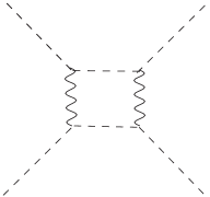
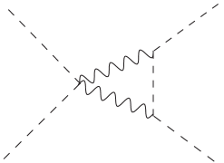
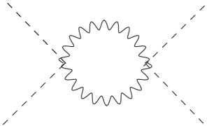
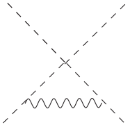
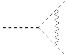
Figure 1: Gauge-dependent diagrams with only light scalars/gauge bosons in the loops, which must contribute zero after infra-red regulation; heavy fields are denoted with a thick line.

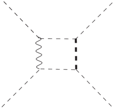
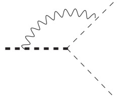
Figure 2: Gauge-dependent diagrams with one heavy scalar in the loop; heavy fields are denoted with a thick line.

Since we take all gauge groups to be unbroken in the limit $\zeta\rightarrow 0$, we may expect that gauge couplings ought to induce no net contribution to $\lambda_{{{\color[rgb]{0,0,0}p}}{{\color[rgb]{0,0,0}q}}{{\color[rgb]{0,0,0}r}}{{\color[rgb]{0,0,0}s}}}$. Indeed, if there are no trilinear couplings in the theory, then this is immediately obvious: the gauge contributions to $\delta\tilde{\lambda}_{{{\color[rgb]{0,0,0}p}}{{\color[rgb]{0,0,0}q}}{{\color[rgb]{0,0,0}r}}{{\color[rgb]{0,0,0}s}}}$ and $\delta\lambda_{{{\color[rgb]{0,0,0}p}}{{\color[rgb]{0,0,0}q}}{{\color[rgb]{0,0,0}r}}{{\color[rgb]{0,0,0}s}}}$ are identical in this case, because the unbroken gauge interactions cannot mix heavy and light fields and certainly the corrections of quartic order in the gauge couplings – i.e. the first row of diagrams in figure 1 – must always be equal. For corrections of quadratic order in the gauge couplings, the second row of diagrams in figure 1 all contain only massless/light fields in the loops, and so we expect them not to contribute. However, once we include trilinear couplings, there are diagrams such as those given in figure 2 which are individually non-zero after infra-red regulation, and so it is possible that there could be some residual dependence on the gauge couplings. However, this cancels out, as we show below.

The individual infra-red safe contributions (it is straightforward to show that the infra-red divergences cancel) are

$$\kappa^{-1}\overline{\delta}_{g^{2}}\tilde{\lambda}_{{{\color[rgb]{0,0,0}p}}{{\color[rgb]{0,0,0}q}}{{\color[rgb]{0,0,0}r}}{{\color[rgb]{0,0,0}s}}}= -\frac{1}{2}\xi g^{a{{\color[rgb]{0,0,0}p}}{{\color[rgb]{0,0,0}t}}}g^{a{{\color[rgb]{0,0,0}q}}{{\color[rgb]{0,0,0}v}}}a_{{{\color[rgb]{0,0,0}t}}{{\color[rgb]{0,0,0}\mathcal{P}}}{{\color[rgb]{0,0,0}r}}}a_{{{\color[rgb]{0,0,0}\mathcal{P}}}{{\color[rgb]{0,0,0}v}}{{\color[rgb]{0,0,0}s}}}\overline{C}_{0}(m_{{\color[rgb]{0,0,0}t}}^{2},m_{{\color[rgb]{0,0,0}\mathcal{P}}}^{2},m_{{\color[rgb]{0,0,0}v}}^{2})+({{\color[rgb]{0,0,0}p}}{{\color[rgb]{0,0,0}q}}{{\color[rgb]{0,0,0}r}}{{\color[rgb]{0,0,0}s}})=-\frac{1}{2}\xi g^{a{{\color[rgb]{0,0,0}p}}{{\color[rgb]{0,0,0}t}}}g^{a{{\color[rgb]{0,0,0}q}}{{\color[rgb]{0,0,0}v}}}a_{{{\color[rgb]{0,0,0}t}}{{\color[rgb]{0,0,0}\mathcal{P}}}{{\color[rgb]{0,0,0}r}}}a_{{{\color[rgb]{0,0,0}\mathcal{P}}}{{\color[rgb]{0,0,0}v}}{{\color[rgb]{0,0,0}s}}}\frac{A_{0}(m_{{\color[rgb]{0,0,0}\mathcal{P}}}^{2})}{m_{{\color[rgb]{0,0,0}\mathcal{P}}}^{4}}+({{\color[rgb]{0,0,0}p}}{{\color[rgb]{0,0,0}q}}{{\color[rgb]{0,0,0}r}}{{\color[rgb]{0,0,0}s}})$$

$$= \,-\frac{1}{8}\xi g^{2}C_{2}({{\color[rgb]{0,0,0}\mathcal{P}}})a_{{{\color[rgb]{0,0,0}\mathcal{P}}}{{\color[rgb]{0,0,0}r}}{{\color[rgb]{0,0,0}s}}}a_{{{\color[rgb]{0,0,0}\mathcal{P}}}{{\color[rgb]{0,0,0}p}}{{\color[rgb]{0,0,0}q}}}\frac{A_{0}(m_{{\color[rgb]{0,0,0}\mathcal{P}}}^{2})}{m_{{\color[rgb]{0,0,0}\mathcal{P}}}^{4}}+({{\color[rgb]{0,0,0}p}}{{\color[rgb]{0,0,0}q}}{{\color[rgb]{0,0,0}r}}{{\color[rgb]{0,0,0}s}}),$$

$$\kappa^{-1}\overline{\delta}_{g^{2}}a_{{{\color[rgb]{0,0,0}\mathcal{P}}}{{\color[rgb]{0,0,0}p}}{{\color[rgb]{0,0,0}q}}}= -\xi g^{a{{\color[rgb]{0,0,0}\mathcal{P}}}{{\color[rgb]{0,0,0}\mathcal{T}}}}g^{a{{\color[rgb]{0,0,0}q}}{{\color[rgb]{0,0,0}n}}}a_{{{\color[rgb]{0,0,0}\mathcal{T}}}{{\color[rgb]{0,0,0}n}}{{\color[rgb]{0,0,0}p}}}\overline{P}_{SS}(m_{{\color[rgb]{0,0,0}\mathcal{T}}}^{2},m_{{\color[rgb]{0,0,0}n}}^{2})-\xi g^{a{{\color[rgb]{0,0,0}\mathcal{P}}}{{\color[rgb]{0,0,0}\mathcal{T}}}}g^{a{{\color[rgb]{0,0,0}p}}{{\color[rgb]{0,0,0}n}}}a_{{{\color[rgb]{0,0,0}\mathcal{T}}}{{\color[rgb]{0,0,0}n}}{{\color[rgb]{0,0,0}q}}}\overline{P}_{SS}(m_{{\color[rgb]{0,0,0}\mathcal{T}}}^{2},m_{{\color[rgb]{0,0,0}n}}^{2})$$

$$= \,\xi g^{a{{\color[rgb]{0,0,0}\mathcal{P}}}{{\color[rgb]{0,0,0}\mathcal{T}}}}g^{a{{\color[rgb]{0,0,0}\mathcal{T}}}{{\color[rgb]{0,0,0}\mathcal{N}}}}a_{{{\color[rgb]{0,0,0}\mathcal{N}}}{{\color[rgb]{0,0,0}p}}{{\color[rgb]{0,0,0}q}}}\frac{A_{0}(m_{{\color[rgb]{0,0,0}\mathcal{T}}}^{2})}{m_{{\color[rgb]{0,0,0}\mathcal{T}}}^{2}}=-\xi g^{2}C_{2}({{\color[rgb]{0,0,0}\mathcal{P}}})a_{{{\color[rgb]{0,0,0}\mathcal{P}}}{{\color[rgb]{0,0,0}p}}{{\color[rgb]{0,0,0}q}}}\frac{A_{0}(m_{{\color[rgb]{0,0,0}\mathcal{P}}}^{2})}{m_{{\color[rgb]{0,0,0}\mathcal{P}}}^{2}},$$

$$\kappa^{-1}\overline{\delta}_{g^{2}}m^{2}_{{{\color[rgb]{0,0,0}\mathcal{P}}}{{\color[rgb]{0,0,0}\mathcal{Q}}}}= -\xi g^{a{{\color[rgb]{0,0,0}\mathcal{P}}}{{\color[rgb]{0,0,0}\mathcal{T}}}}g^{a{{\color[rgb]{0,0,0}\mathcal{Q}}}{{\color[rgb]{0,0,0}\mathcal{T}}}}A_{0}(m_{{\color[rgb]{0,0,0}\mathcal{T}}}^{2})=-\xi\delta_{{{\color[rgb]{0,0,0}\mathcal{P}}}{{\color[rgb]{0,0,0}\mathcal{Q}}}}g^{2}C_{2}({{\color[rgb]{0,0,0}\mathcal{P}}})A_{0}(m_{{\color[rgb]{0,0,0}\mathcal{P}}}^{2}),$$ (3.11)

where $g^{2}$ is the relevant gauge coupling and $C_{2}({{\color[rgb]{0,0,0}\mathcal{P}}})$ is the quadratic Casimir of the corresponding representation of heavy field ${{\color[rgb]{0,0,0}\mathcal{P}}}$. For each term we have used gauge invariance to simplify the expressions. We see that all of these contributions are proportional to the gauge-fixing parameter $\xi$, which tells us that the total contribution must vanish; this would not have been obvious if we had worked in the Feynman gauge (but of course would be in the Landau gauge!). Indeed, combining the above contributions as in eq. (3.2) gives

$$\overline{\delta}_{g^{2}}\tilde{\lambda}_{{{\color[rgb]{0,0,0}p}}{{\color[rgb]{0,0,0}q}}{{\color[rgb]{0,0,0}r}}{{\color[rgb]{0,0,0}s}}}-\bigg{[}\frac{1}{4m_{{\color[rgb]{0,0,0}\mathcal{P}}}^{2}}a_{{{\color[rgb]{0,0,0}\mathcal{P}}}{{\color[rgb]{0,0,0}r}}{{\color[rgb]{0,0,0}s}}}\overline{\delta}_{g^{2}}a_{{{\color[rgb]{0,0,0}\mathcal{P}}}{{\color[rgb]{0,0,0}p}}{{\color[rgb]{0,0,0}q}}}-\frac{1}{8m_{{\color[rgb]{0,0,0}\mathcal{P}}}^{2}m_{{\color[rgb]{0,0,0}\mathcal{Q}}}^{2}}a_{{{\color[rgb]{0,0,0}\mathcal{P}}}{{\color[rgb]{0,0,0}r}}{{\color[rgb]{0,0,0}s}}}a_{{{\color[rgb]{0,0,0}\mathcal{Q}}}{{\color[rgb]{0,0,0}p}}{{\color[rgb]{0,0,0}q}}}\overline{\delta}_{g^{2}}m_{{{\color[rgb]{0,0,0}\mathcal{P}}}{{\color[rgb]{0,0,0}\mathcal{Q}}}}^{2}+({{\color[rgb]{0,0,0}p}}{{\color[rgb]{0,0,0}q}}{{\color[rgb]{0,0,0}r}}{{\color[rgb]{0,0,0}s}})\bigg{]}= \ 0\,.$$ (3.12)

Hence we can indeed neglect gauge contributions at one loop, as there is no gauge contribution to $\delta m_{{{\color[rgb]{0,0,0}p}}{{\color[rgb]{0,0,0}\mathcal{P}}}}^{2}$ and $\delta_{g^{2}}Z^{H}=\delta_{g^{2}}Z^{L}$. However, it is important to note that we require all of the separate pieces together in order to cancel the gauge dependence, which will be relevant in section 4.

3.4 Trilinear couplings and higher-dimensional operators

We end this section by considering the case of non-vanishing trilinear couplings between light states, i.e. $a_{{{\color[rgb]{0,0,0}p}}{{\color[rgb]{0,0,0}q}}{{\color[rgb]{0,0,0}r}}}\neq 0$. Such couplings result in new divergent diagrams compared to the case considered in appendix C (where we demonstrate the cancellation of all IR divergences when $a_{{{\color[rgb]{0,0,0}p}}{{\color[rgb]{0,0,0}q}}{{\color[rgb]{0,0,0}r}}}=0$). Indeed, considering the different contributions appearing in equation (3.2), one can observe that several divergent terms in the high-energy part of the matching do not seem to cancel out with any term in the low-energy part, namely

$$\kappa\,\bigg{\{} -\frac{1}{2}\tilde{\lambda}_{{{\color[rgb]{0,0,0}p}}{{\color[rgb]{0,0,0}q}}{{\color[rgb]{0,0,0}x}}{{\color[rgb]{0,0,0}\mathcal{Y}}}}a_{{{\color[rgb]{0,0,0}r}}{{\color[rgb]{0,0,0}x}}{{\color[rgb]{0,0,0}z}}}a_{{{\color[rgb]{0,0,0}s}}{{\color[rgb]{0,0,0}\mathcal{Y}}}{{\color[rgb]{0,0,0}z}}}\frac{P_{SS}(m^{2}_{{\color[rgb]{0,0,0}x}},m^{2}_{{\color[rgb]{0,0,0}z}})}{m_{{{\color[rgb]{0,0,0}\mathcal{Y}}}}^{2}}+\frac{1}{2}a_{{{\color[rgb]{0,0,0}p}}{{\color[rgb]{0,0,0}\mathcal{X}}}{{\color[rgb]{0,0,0}\mathcal{Y}}}}a_{{{\color[rgb]{0,0,0}q}}{{\color[rgb]{0,0,0}\mathcal{X}}}{{\color[rgb]{0,0,0}z}}}a_{{{\color[rgb]{0,0,0}r}}{{\color[rgb]{0,0,0}\mathcal{Y}}}{{\color[rgb]{0,0,0}u}}}a_{{{\color[rgb]{0,0,0}s}}{{\color[rgb]{0,0,0}z}}{{\color[rgb]{0,0,0}u}}}\frac{P_{SS}(m^{2}_{{\color[rgb]{0,0,0}z}},m^{2}_{{\color[rgb]{0,0,0}u}})}{m_{{{\color[rgb]{0,0,0}\mathcal{X}}}}^{2}m_{{{\color[rgb]{0,0,0}\mathcal{Y}}}}^{2}}$$

$$-\frac{1}{4}a_{{{\color[rgb]{0,0,0}\mathcal{P}}}{{\color[rgb]{0,0,0}p}}{{\color[rgb]{0,0,0}q}}}\tilde{\lambda}_{{{\color[rgb]{0,0,0}\mathcal{P}}}{{\color[rgb]{0,0,0}r}}{{\color[rgb]{0,0,0}x}}{{\color[rgb]{0,0,0}y}}}a_{{{\color[rgb]{0,0,0}s}}{{\color[rgb]{0,0,0}x}}{{\color[rgb]{0,0,0}y}}}\frac{P_{SS}(m_{{\color[rgb]{0,0,0}x}}^{2},m_{{\color[rgb]{0,0,0}y}}^{2})}{m_{{{\color[rgb]{0,0,0}\mathcal{P}}}}^{2}}+\frac{1}{2}a_{{{\color[rgb]{0,0,0}\mathcal{P}}}{{\color[rgb]{0,0,0}p}}{{\color[rgb]{0,0,0}q}}}a_{{{\color[rgb]{0,0,0}\mathcal{P}}}{{\color[rgb]{0,0,0}\mathcal{X}}}{{\color[rgb]{0,0,0}y}}}a_{{{\color[rgb]{0,0,0}r}}{{\color[rgb]{0,0,0}\mathcal{X}}}{{\color[rgb]{0,0,0}z}}}a_{{{\color[rgb]{0,0,0}s}}{{\color[rgb]{0,0,0}y}}{{\color[rgb]{0,0,0}z}}}\frac{P_{SS}(m_{{\color[rgb]{0,0,0}y}}^{2},m_{{\color[rgb]{0,0,0}z}}^{2})}{m_{{{\color[rgb]{0,0,0}\mathcal{P}}}}^{2}m_{{{\color[rgb]{0,0,0}\mathcal{X}}}}^{2}}$$

$$-\frac{1}{12}a_{{{\color[rgb]{0,0,0}\mathcal{P}}}{{\color[rgb]{0,0,0}x}}{{\color[rgb]{0,0,0}y}}}a_{{{\color[rgb]{0,0,0}p}}{{\color[rgb]{0,0,0}x}}{{\color[rgb]{0,0,0}y}}}\bigg{[}\tilde{\lambda}_{{{\color[rgb]{0,0,0}\mathcal{P}}}{{\color[rgb]{0,0,0}q}}{{\color[rgb]{0,0,0}r}}{{\color[rgb]{0,0,0}s}}}-\frac{3}{m_{{{\color[rgb]{0,0,0}\mathcal{Q}}}}^{2}}a_{{{\color[rgb]{0,0,0}\mathcal{P}}}{{\color[rgb]{0,0,0}\mathcal{Q}}}{{\color[rgb]{0,0,0}q}}}a_{{{\color[rgb]{0,0,0}\mathcal{Q}}}{{\color[rgb]{0,0,0}r}}{{\color[rgb]{0,0,0}s}}}\bigg{]}\frac{P_{SS}(m_{{\color[rgb]{0,0,0}x}}^{2},m_{{\color[rgb]{0,0,0}y}}^{2})}{m_{{{\color[rgb]{0,0,0}\mathcal{P}}}}^{2}}$$

$$-\frac{1}{2}a_{{{\color[rgb]{0,0,0}p}}{{\color[rgb]{0,0,0}\mathcal{X}}}{{\color[rgb]{0,0,0}y}}}a_{{{\color[rgb]{0,0,0}q}}{{\color[rgb]{0,0,0}\mathcal{X}}}{{\color[rgb]{0,0,0}z}}}a_{{{\color[rgb]{0,0,0}r}}{{\color[rgb]{0,0,0}y}}{{\color[rgb]{0,0,0}u}}}a_{{{\color[rgb]{0,0,0}s}}{{\color[rgb]{0,0,0}z}}{{\color[rgb]{0,0,0}u}}}\frac{P_{SS}(m_{{\color[rgb]{0,0,0}z}}^{2},m_{{\color[rgb]{0,0,0}u}}^{2})}{m_{{{\color[rgb]{0,0,0}\mathcal{X}}}}^{4}}+({{\color[rgb]{0,0,0}p}}{{\color[rgb]{0,0,0}q}}{{\color[rgb]{0,0,0}r}}{{\color[rgb]{0,0,0}s}})\bigg{\}}\,.$$ (3.13)

Note that all these terms involve one, or two, trilinear couplings between light scalars. Moreover, one may observe that these remaining terms are all proportional to a $P_{SS}$ loop function – in some cases this $P_{SS}$ being obtained from the expansion of a $C_{0}$ or $D_{0}$ function – while it can be shown that divergent terms with $C_{0}(m_{x}^{2},m_{y}^{2},m_{z}^{2})$ or $D_{0}(m_{x}^{2},m_{y}^{2},m_{z}^{2},m_{u}^{2})$ – with all masses being light – do cancel out.

If we reason with orders of magnitude, it is natural to assume that couplings $a_{{{\color[rgb]{0,0,0}\mathcal{P}}}{{\color[rgb]{0,0,0}q}}{{\color[rgb]{0,0,0}r}}}$ and $a_{{{\color[rgb]{0,0,0}\mathcal{P}}}{{\color[rgb]{0,0,0}\mathcal{Q}}}{{\color[rgb]{0,0,0}r}}}$ are of the order of a heavy mass, say $M$, times numerical factors of $\mathcal{O}(1)$. From this we can easily see that all of the above terms are of order $a_{{{\color[rgb]{0,0,0}p}}{{\color[rgb]{0,0,0}q}}{{\color[rgb]{0,0,0}r}}}/M$ (and even $(a_{{{\color[rgb]{0,0,0}p}}{{\color[rgb]{0,0,0}q}}{{\color[rgb]{0,0,0}r}}}/M)^{2}$ for the last one). As we could expect $a_{{{\color[rgb]{0,0,0}p}}{{\color[rgb]{0,0,0}q}}{{\color[rgb]{0,0,0}r}}}$ to be of the order of a light mass (e.g. $m_{{{\color[rgb]{0,0,0}p}}}\sim\zeta$), it would seem natural that the above terms be suppressed at least as $\mathcal{O}(\zeta/M)$ – and therefore also go to zero in the limit $\zeta\to 0$. The finite part of the matching is then exactly the same as that obtained previously.

However, one can still want to understand what happens if the trilinear couplings between light states are not of the order of $\zeta$. Having very large trilinear couplings in the low-energy theory could potentially cause a breakdown of perturbativity and/or unitarity, as well as expectation values in the low-energy theory of the order of the heavy masses. Nevertheless, it is actually still possible in such a case to cancel all of the IR divergences, by taking into account higher-dimensional operators.

More specifically, one can deduce from the form of the divergent terms in equation (3.4) that the required new operators are a dimension-5 operator $c_{5}^{{{\color[rgb]{0,0,0}p}}{{\color[rgb]{0,0,0}q}}{{\color[rgb]{0,0,0}r}}{{\color[rgb]{0,0,0}s}}{{\color[rgb]{0,0,0}t}}}\phi_{{\color[rgb]{0,0,0}p}}\phi_{{\color[rgb]{0,0,0}q}}\phi_{{\color[rgb]{0,0,0}r}}\phi_{{\color[rgb]{0,0,0}s}}\phi_{{\color[rgb]{0,0,0}t}}$ and a dimension-6 operator $k_{6}^{{{\color[rgb]{0,0,0}p}}{{\color[rgb]{0,0,0}q}}{{\color[rgb]{0,0,0}r}}{{\color[rgb]{0,0,0}s}}}\phi_{{\color[rgb]{0,0,0}p}}\phi_{{\color[rgb]{0,0,0}q}}\partial_{\mu}\phi_{{\color[rgb]{0,0,0}r}}\partial^{\mu}\phi_{{\color[rgb]{0,0,0}s}}$ (a correction to the kinetic term of the scalars). The former will cancel out with the first three lines of eq. (3.4), while the latter compensates the last remaining term.

3.4.1 Higher-dimensional operators in a toy model

To illustrate how to address the additional terms of eq. (3.4), it will prove useful to first consider a simple toy example, with only two scalars – one light $L$ and one heavy $H$ – in the high-energy theory. The Lagrangian of such a model reads

$$\mathcal{L}_{\text{HET}}\supset -\frac{1}{2}m_{L}^{2}L^{2}-\frac{1}{2}m_{H}^{2}H^{2}-\frac{1}{6}a_{LLL}L^{3}-\frac{1}{2}a_{LLH}L^{2}H-\frac{1}{2}a_{LHH}LH^{2}-\frac{1}{6}a_{HHH}H^{3}$$

$$-\frac{1}{24}\tilde{\lambda}_{LLLL}L^{4}-\frac{1}{6}\tilde{\lambda}_{LLLH}L^{3}H-\frac{1}{4}\tilde{\lambda}_{LLHH}L^{2}H^{2}-\frac{1}{6}\tilde{\lambda}_{LHHH}LH^{3}-\frac{1}{24}\tilde{\lambda}_{HHHH}H^{4}$$ (3.14)

Performing the one-loop matching of the quartic coupling $\lambda^{LLLL}$ as previously, we obtain

$$\lambda_{LLLL}+\delta\lambda_{LLLL}= \,\tilde{\lambda}_{LLLL}-\frac{3}{m_{H}^{2}}(a_{LLH})^{2}+\delta\tilde{\lambda}_{LLLL}-\frac{6a_{LLH}}{m_{H}^{2}}\delta a_{LLH}+\frac{3(a_{LLH})^{2}}{m_{H}^{4}}\delta m_{HH}^{2}\,.$$ (3.15)

The IR-divergent terms left on the right-hand side of the matching are then

$$-\kappa\bigg{[}20\frac{a_{LLH}a_{LLL}\tilde{\lambda}_{LLLH}}{m_{H}^{2}}-30\frac{a_{LHH}(a_{LLH})^{2}a_{LLL}}{m_{H}^{4}}+12\frac{(a_{LLH})^{2}(a_{LLL})^{2}}{m_{H}^{4}}\bigg{]}P_{SS}(m_{L}^{2},m_{L}^{2})\,,$$ (3.16)

and correspond to the types of diagrams shown in figure 3 (recall that $\kappa$ is the loop factor). One can expect the divergent terms in equation (3.16) to correspond to diagrams in the EFT similar to those in figure 3, but with the dashed lines corresponding to heavy propagators contracted to points. In particular, the low-energy diagrams corresponding to diagrams $(i)$ and $(iii)-(vi)$ in figure 3 will involve a coupling between five scalars, while the diagram corresponding to $(ii)$ will involve a dimension-6 coupling between four scalars, suppressed by $m_{H}^{4}$. We define the corresponding operators as

$$\mathcal{L}_{\text{EFT}}\supset-\frac{1}{5!}c_{5}^{LLLLL}L^{5}-\frac{1}{4}k_{6}^{LLLL}L^{2}(\partial_{\mu}L)^{2}$$ (3.17)

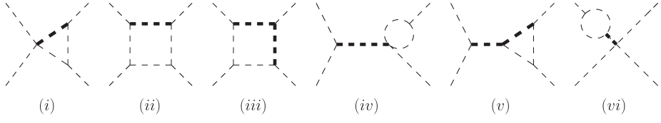
Figure 3: Types of diagrams that contribute to the high-energy part of the matching of quartic couplings and that contain divergences only regulated when including higher-dimensional operators in the low-energy theory. Bold lines denote heavy propagators.

Before deriving the expressions of these two higher-dimensional operators, it is important to note that they will only appear in one-loop diagrams in the low-energy part of the matching and therefore it will suffice for the discussion at hand here to obtain their tree-level expressions. For the dimension-5 coupling, two different sorts of diagrams contribute to its tree-level expression, as shown in figure 6. We find

$$c_{5}^{LLLLL}=-10\frac{a_{LLH}\tilde{\lambda}_{LLLH}}{m_{H}^{2}}+15\frac{a_{LHH}(a_{LLH})^{2}}{m_{H}^{4}}\,.$$ (3.18)

The dimension-6 operator is obtained from similar diagrams as the tree-level threshold corrections to $\lambda_{LLLL}$, but taking the second order in the $p^{2}/m_{H}^{2}$ expansion of the heavy propagator. Finally, we find

$$k_{6}^{LLLL}=-\frac{2}{m_{H}^{4}}(a_{LLH})^{2}\,.$$ (3.19)

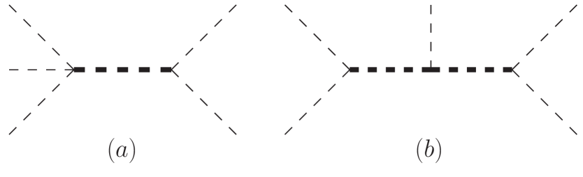
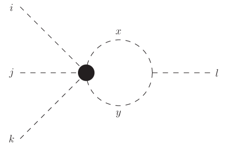
Figure 4: Diagrams in the high-energy theory that contribute to the tree-level expression of $c_{5}^{LLLLL}$ (or in general of $c_{5}^{{{\color[rgb]{0,0,0}p}}{{\color[rgb]{0,0,0}q}}{{\color[rgb]{0,0,0}r}}{{\color[rgb]{0,0,0}s}}{{\color[rgb]{0,0,0}t}}}$). Bold lines denote heavy propagators.

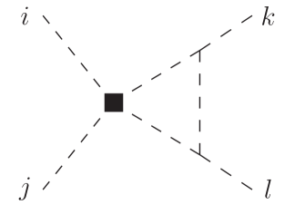
Figure 5: New diagram in the low-energy theory part of the matching of the scalar quartic coupling, involving a dimension-5 scalar operator.

Figure 6: New diagram involving a dimension-6 operator – denoted by a black square – in the low-energy side of the one-loop matching.

One can then compute the new contributions to $\delta\lambda_{LLLL}$ arising from diagrams involving $c_{5}^{LLLLL}$ and $k_{6}^{LLLL}$ – shown respectively in figures 6 and 6 – and one finds

$$\kappa^{-1}\delta\lambda_{LLLL}\supset 2c_{5}^{LLLLL}a_{LLL}P_{SS}(m_{L}^{2},m_{L}^{2})+6k_{6}^{LLLL}(a_{LLL})^{2}\big{[}P_{SS}(m_{L}^{2},m_{L}^{2})-m_{L}^{2}C_{0}(m_{L}^{2},m_{L}^{2},m_{L}^{2})\big{]}\,.$$ (3.20)

Note that the last term within parentheses in the above expression is regular in the limit $m_{L}\to 0$. Using the tree-level expressions in eqs. (3.18) and (3.19), we can rewrite these contributions as

$$\kappa^{-1}\delta\lambda_{LLLL}\supset -\bigg{[}20\frac{a_{LLH}a_{LLL}\tilde{\lambda}_{LLLH}}{m_{H}^{2}}-30\frac{a_{LHH}(a_{LLH})^{2}a_{LLL}}{m_{H}^{4}}\bigg{]}P_{SS}(m_{L}^{2},m_{L}^{2})$$

$$-12\frac{(a_{LLH})^{2}(a_{LLL})^{2}}{m_{H}^{4}}\big{[}P_{SS}(m_{L}^{2},m_{L}^{2})+\text{reg.}\big{]}\,,$$ (3.21)

which exactly correspond to the divergent terms in equation (3.16).

3.4.2 Discussion of the dimension-5 operator for a general theory

We now investigate the corresponding higher-order operators in the context of the matching of generic theories. We denote these two couplings as $c_{5}^{{{\color[rgb]{0,0,0}p}}{{\color[rgb]{0,0,0}q}}{{\color[rgb]{0,0,0}r}}{{\color[rgb]{0,0,0}s}}{{\color[rgb]{0,0,0}t}}}$ and $k_{6}^{{{\color[rgb]{0,0,0}p}}{{\color[rgb]{0,0,0}q}}{{\color[rgb]{0,0,0}r}}{{\color[rgb]{0,0,0}s}}}$, respectively, and we define the corresponding Lagrangian terms as

$$\mathcal{L}_{\text{EFT}}\supset-\frac{1}{5!}c_{5}^{{{\color[rgb]{0,0,0}p}}{{\color[rgb]{0,0,0}q}}{{\color[rgb]{0,0,0}r}}{{\color[rgb]{0,0,0}s}}{{\color[rgb]{0,0,0}t}}}\phi_{{\color[rgb]{0,0,0}p}}\phi_{{\color[rgb]{0,0,0}q}}\phi_{{\color[rgb]{0,0,0}r}}\phi_{{\color[rgb]{0,0,0}s}}\phi_{{\color[rgb]{0,0,0}t}}-\frac{1}{4}k_{6}^{{{\color[rgb]{0,0,0}p}}{{\color[rgb]{0,0,0}q}}{{\color[rgb]{0,0,0}r}}{{\color[rgb]{0,0,0}s}}}\phi_{{\color[rgb]{0,0,0}p}}\phi_{{\color[rgb]{0,0,0}q}}\partial_{\mu}\phi_{{\color[rgb]{0,0,0}r}}\partial^{\mu}\phi_{{\color[rgb]{0,0,0}s}}\,.$$ (3.22)

For both operators, we will first derive their (tree-level) expression in terms of couplings of the high-energy theory, before showing how their inclusion allows to cancel all remaining IR divergences in the one-loop matching of the quartic coupling.

We must first derive the tree-level expression of the new dimension-5 scalar $c_{5}^{{{\color[rgb]{0,0,0}p}}{{\color[rgb]{0,0,0}q}}{{\color[rgb]{0,0,0}r}}{{\color[rgb]{0,0,0}s}}{{\color[rgb]{0,0,0}t}}}$ operator that is generated in the low-energy theory, by repeating the matching of effective actions done in equation (2.3). Keeping now terms with five scalars, the Lagrangian of the high-energy theory contains

$$\mathcal{L}_{\text{eff}}[\Phi]\supset \ \frac{1}{12m_{{{\color[rgb]{0,0,0}\mathcal{P}}}}^{2}}a_{{{\color[rgb]{0,0,0}\mathcal{P}}}{{\color[rgb]{0,0,0}p}}{{\color[rgb]{0,0,0}q}}}\tilde{\lambda}_{{{\color[rgb]{0,0,0}\mathcal{P}}}{{\color[rgb]{0,0,0}r}}{{\color[rgb]{0,0,0}s}}{{\color[rgb]{0,0,0}t}}}\Phi_{{\color[rgb]{0,0,0}p}}\Phi_{{\color[rgb]{0,0,0}q}}\Phi_{{\color[rgb]{0,0,0}r}}\Phi_{{\color[rgb]{0,0,0}s}}\Phi_{{\color[rgb]{0,0,0}t}}-\frac{1}{8m_{{{\color[rgb]{0,0,0}\mathcal{P}}}}^{2}m_{{{\color[rgb]{0,0,0}\mathcal{Q}}}}^{2}}a_{{{\color[rgb]{0,0,0}\mathcal{P}}}{{\color[rgb]{0,0,0}p}}{{\color[rgb]{0,0,0}q}}}a_{{{\color[rgb]{0,0,0}\mathcal{P}}}{{\color[rgb]{0,0,0}\mathcal{Q}}}{{\color[rgb]{0,0,0}r}}}a_{{{\color[rgb]{0,0,0}\mathcal{Q}}}{{\color[rgb]{0,0,0}s}}{{\color[rgb]{0,0,0}t}}}\Phi_{{\color[rgb]{0,0,0}p}}\Phi_{{\color[rgb]{0,0,0}q}}\Phi_{{\color[rgb]{0,0,0}r}}\Phi_{{\color[rgb]{0,0,0}s}}\Phi_{{\color[rgb]{0,0,0}t}}+\cdots$$ (3.23)

Identifying this with the definition of $c_{5}$ in eq. (3.22), and symmetrising the indices, we obtain for the tree-level matching of $c_{5}$

$$c_{5}^{{{\color[rgb]{0,0,0}p}}{{\color[rgb]{0,0,0}q}}{{\color[rgb]{0,0,0}r}}{{\color[rgb]{0,0,0}s}}{{\color[rgb]{0,0,0}t}}}= -\frac{1}{12m_{{{\color[rgb]{0,0,0}\mathcal{P}}}}^{2}}a_{{{\color[rgb]{0,0,0}\mathcal{P}}}{{\color[rgb]{0,0,0}p}}{{\color[rgb]{0,0,0}q}}}\bigg{[}\tilde{\lambda}_{{{\color[rgb]{0,0,0}\mathcal{P}}}{{\color[rgb]{0,0,0}r}}{{\color[rgb]{0,0,0}s}}{{\color[rgb]{0,0,0}t}}}-\frac{3}{2m_{{{\color[rgb]{0,0,0}\mathcal{Q}}}}^{2}}a_{{{\color[rgb]{0,0,0}\mathcal{P}}}{{\color[rgb]{0,0,0}\mathcal{Q}}}{{\color[rgb]{0,0,0}r}}}a_{{{\color[rgb]{0,0,0}\mathcal{Q}}}{{\color[rgb]{0,0,0}s}}{{\color[rgb]{0,0,0}t}}}\bigg{]}+({{\color[rgb]{0,0,0}p}}{{\color[rgb]{0,0,0}q}}{{\color[rgb]{0,0,0}r}}{{\color[rgb]{0,0,0}s}}{{\color[rgb]{0,0,0}t}})\,.$$ (3.24)

The dimension-5 operator gives rise to a new type of diagrams, shown in figure 6, contributing to the low-energy part of the matching of the quartic couplings. The additional terms in $\delta\lambda_{{{\color[rgb]{0,0,0}p}}{{\color[rgb]{0,0,0}q}}{{\color[rgb]{0,0,0}r}}{{\color[rgb]{0,0,0}s}}}$ read

$$\kappa^{-1}\delta\lambda_{{{\color[rgb]{0,0,0}p}}{{\color[rgb]{0,0,0}q}}{{\color[rgb]{0,0,0}r}}{{\color[rgb]{0,0,0}s}}}\supset \ \frac{1}{12}c_{5}^{{{\color[rgb]{0,0,0}p}}{{\color[rgb]{0,0,0}q}}{{\color[rgb]{0,0,0}r}}{{\color[rgb]{0,0,0}x}}{{\color[rgb]{0,0,0}y}}}a_{{{\color[rgb]{0,0,0}x}}{{\color[rgb]{0,0,0}y}}{{\color[rgb]{0,0,0}s}}}P_{SS}(m_{{\color[rgb]{0,0,0}x}}^{2},m_{{\color[rgb]{0,0,0}y}}^{2})+({{\color[rgb]{0,0,0}p}}{{\color[rgb]{0,0,0}q}}{{\color[rgb]{0,0,0}r}}{{\color[rgb]{0,0,0}s}})$$

$$= -\frac{5}{6m_{{{\color[rgb]{0,0,0}\mathcal{P}}}}^{2}}a_{{{\color[rgb]{0,0,0}\mathcal{P}}}{{\color[rgb]{0,0,0}p}}{{\color[rgb]{0,0,0}q}}}a_{{{\color[rgb]{0,0,0}x}}{{\color[rgb]{0,0,0}y}}{{\color[rgb]{0,0,0}s}}}\bigg{[}\tilde{\lambda}_{{{\color[rgb]{0,0,0}\mathcal{P}}}{{\color[rgb]{0,0,0}r}}{{\color[rgb]{0,0,0}x}}{{\color[rgb]{0,0,0}y}}}-\frac{3}{2m_{{{\color[rgb]{0,0,0}\mathcal{Q}}}}^{2}}a_{{{\color[rgb]{0,0,0}\mathcal{P}}}{{\color[rgb]{0,0,0}\mathcal{Q}}}{{\color[rgb]{0,0,0}r}}}a_{{{\color[rgb]{0,0,0}\mathcal{Q}}}{{\color[rgb]{0,0,0}x}}{{\color[rgb]{0,0,0}y}}}\bigg{]}P_{SS}(m_{{\color[rgb]{0,0,0}x}}^{2},m_{{\color[rgb]{0,0,0}y}}^{2})+({{\color[rgb]{0,0,0}p}}{{\color[rgb]{0,0,0}q}}{{\color[rgb]{0,0,0}r}}{{\color[rgb]{0,0,0}s}})\,.$$ (3.25)

Using permutations of indices, it can be shown that the terms in equation (3.4.2) match exactly the three first lines of equation (3.4). Only the last term

$$-\frac{1}{2}a_{{{\color[rgb]{0,0,0}p}}{{\color[rgb]{0,0,0}\mathcal{X}}}{{\color[rgb]{0,0,0}y}}}a_{{{\color[rgb]{0,0,0}q}}{{\color[rgb]{0,0,0}\mathcal{X}}}{{\color[rgb]{0,0,0}z}}}a_{{{\color[rgb]{0,0,0}r}}{{\color[rgb]{0,0,0}y}}{{\color[rgb]{0,0,0}u}}}a_{{{\color[rgb]{0,0,0}s}}{{\color[rgb]{0,0,0}z}}{{\color[rgb]{0,0,0}u}}}\frac{P_{SS}(m_{{\color[rgb]{0,0,0}z}}^{2},m_{{\color[rgb]{0,0,0}u}}^{2})}{m_{{{\color[rgb]{0,0,0}\mathcal{X}}}}^{4}}+({{\color[rgb]{0,0,0}p}}{{\color[rgb]{0,0,0}q}}{{\color[rgb]{0,0,0}r}}{{\color[rgb]{0,0,0}s}})\,,$$

is left, and has to be cancelled out by the dimension-6 operator defined in equation (3.22).

3.4.3 Discussion of the dimension-6 operator for a general theory

We start by deriving the (tree-level) matching condition for this coupling, using once again the equation of motion for the heavy fields, and we have

$$\mathcal{L}_{\text{eff}}[\Phi] \supset\frac{1}{8}\frac{a_{{{\color[rgb]{0,0,0}\mathcal{P}}}{{\color[rgb]{0,0,0}p}}{{\color[rgb]{0,0,0}q}}}a_{{{\color[rgb]{0,0,0}\mathcal{P}}}{{\color[rgb]{0,0,0}r}}{{\color[rgb]{0,0,0}s}}}}{m_{{{\color[rgb]{0,0,0}\mathcal{P}}}}^{4}}\partial_{\mu}\big{(}\Phi_{{\color[rgb]{0,0,0}p}}\Phi_{{\color[rgb]{0,0,0}q}}\big{)}\partial^{\mu}\big{(}\Phi_{{\color[rgb]{0,0,0}r}}\Phi_{{\color[rgb]{0,0,0}s}}\big{)}+\cdots=\frac{1}{2}\frac{a_{{{\color[rgb]{0,0,0}\mathcal{P}}}{{\color[rgb]{0,0,0}p}}{{\color[rgb]{0,0,0}r}}}a_{{{\color[rgb]{0,0,0}\mathcal{P}}}{{\color[rgb]{0,0,0}q}}{{\color[rgb]{0,0,0}s}}}}{m_{{{\color[rgb]{0,0,0}\mathcal{P}}}}^{4}}\Phi_{{\color[rgb]{0,0,0}p}}\Phi_{{\color[rgb]{0,0,0}q}}\partial_{\mu}\Phi_{{\color[rgb]{0,0,0}r}}\partial^{\mu}\Phi_{{\color[rgb]{0,0,0}s}}+\cdots$$ (3.26)

Matching the Lagrangians of the high- and low-energy theory at tree level, we obtain

$$k_{6}^{{{\color[rgb]{0,0,0}p}}{{\color[rgb]{0,0,0}q}}{{\color[rgb]{0,0,0}r}}{{\color[rgb]{0,0,0}s}}}=-\frac{2}{m_{{{\color[rgb]{0,0,0}\mathcal{P}}}}^{4}}a_{{{\color[rgb]{0,0,0}\mathcal{P}}}{{\color[rgb]{0,0,0}p}}{{\color[rgb]{0,0,0}r}}}a_{{{\color[rgb]{0,0,0}\mathcal{P}}}{{\color[rgb]{0,0,0}q}}{{\color[rgb]{0,0,0}s}}}\,.$$ (3.27)

In turn, we find the following Feynman rule for the dimension-6 coupling

The new type of diagrams in the low-energy theory that will cancel the remaining divergence is shown in figure 6. From these, we have a contribution to $\delta\lambda_{{{\color[rgb]{0,0,0}p}}{{\color[rgb]{0,0,0}q}}{{\color[rgb]{0,0,0}r}}{{\color[rgb]{0,0,0}s}}}$

$$\kappa^{-1}\delta\lambda_{{{\color[rgb]{0,0,0}p}}{{\color[rgb]{0,0,0}q}}{{\color[rgb]{0,0,0}r}}{{\color[rgb]{0,0,0}s}}}\supset \ \frac{1}{4}k_{6}^{{{\color[rgb]{0,0,0}p}}{{\color[rgb]{0,0,0}q}}{{\color[rgb]{0,0,0}x}}{{\color[rgb]{0,0,0}y}}}a_{{{\color[rgb]{0,0,0}r}}{{\color[rgb]{0,0,0}x}}{{\color[rgb]{0,0,0}z}}}a_{{{\color[rgb]{0,0,0}s}}{{\color[rgb]{0,0,0}y}}{{\color[rgb]{0,0,0}z}}}\big{(}P_{SS}(m_{{\color[rgb]{0,0,0}y}}^{2},m_{{\color[rgb]{0,0,0}z}}^{2})-m_{{\color[rgb]{0,0,0}x}}^{2}C_{0}(m_{{\color[rgb]{0,0,0}x}}^{2},m_{{\color[rgb]{0,0,0}y}}^{2},m_{{\color[rgb]{0,0,0}z}}^{2})\big{)}+({{\color[rgb]{0,0,0}p}}{{\color[rgb]{0,0,0}q}}{{\color[rgb]{0,0,0}r}}{{\color[rgb]{0,0,0}s}})$$

$$= -\frac{1}{2m_{{{\color[rgb]{0,0,0}\mathcal{P}}}}^{4}}a_{{{\color[rgb]{0,0,0}\mathcal{P}}}{{\color[rgb]{0,0,0}p}}{{\color[rgb]{0,0,0}x}}}a_{{{\color[rgb]{0,0,0}\mathcal{P}}}{{\color[rgb]{0,0,0}q}}{{\color[rgb]{0,0,0}y}}}a_{{{\color[rgb]{0,0,0}r}}{{\color[rgb]{0,0,0}x}}{{\color[rgb]{0,0,0}z}}}a_{{{\color[rgb]{0,0,0}s}}{{\color[rgb]{0,0,0}y}}{{\color[rgb]{0,0,0}z}}}\big{(}P_{SS}(m_{{\color[rgb]{0,0,0}y}}^{2},m_{{\color[rgb]{0,0,0}z}}^{2})-m_{{\color[rgb]{0,0,0}x}}^{2}C_{0}(m_{{\color[rgb]{0,0,0}x}}^{2},m_{{\color[rgb]{0,0,0}y}}^{2},m_{{\color[rgb]{0,0,0}z}}^{2})\big{)}+({{\color[rgb]{0,0,0}p}}{{\color[rgb]{0,0,0}q}}{{\color[rgb]{0,0,0}r}}{{\color[rgb]{0,0,0}s}}),$$ (3.28)

where for the second line, we used the matching in equation (3.27). The first term within parentheses in the equation (3.4.3) exactly cancels the last divergent term in equation (3.4), while the second term is regular in the limit $m_{{\color[rgb]{0,0,0}x}}^{2}\rightarrow 0$.

4 Non-minimal counterterm approach

In the derivation of section 3.2 we used the running (${\overline{\rm MS}}$ or ${\overline{\rm DR}^{\prime}}$) parameters of the high-energy theory as inputs. However, we may prefer to define our matching scale in terms of the loop-corrected masses and mixings, for example in high-scale/split SUSY cases we can typically choose to adjust $m_{H_{u}}^{2},m_{H_{d}}^{2},B_{\mu}$ and also the $Z$-counterterms. In other words, we can allow new finite corrections to the counterterms, which we denote $\delta_{ct}Z,\,\delta_{ct}m^{2}$:

$$\Gamma[\Phi]= \frac{1}{2}\big{(}\delta_{{{\color[rgb]{0,0,0}i}}{{\color[rgb]{0,0,0}j}}}-\Pi_{{{\color[rgb]{0,0,0}i}}{{\color[rgb]{0,0,0}j}}}^{\prime}(0)+\delta_{ct}Z_{{{\color[rgb]{0,0,0}i}}{{\color[rgb]{0,0,0}j}}}\big{)}\partial_{\mu}\Phi_{{\color[rgb]{0,0,0}i}}\partial^{\mu}\Phi_{{\color[rgb]{0,0,0}j}}-\frac{1}{2}\big{(}m^{2}_{{{\color[rgb]{0,0,0}i}}}\delta_{{{\color[rgb]{0,0,0}i}}{{\color[rgb]{0,0,0}j}}}+\Pi_{{{\color[rgb]{0,0,0}i}}{{\color[rgb]{0,0,0}j}}}(0)+\delta_{ct}m_{{{\color[rgb]{0,0,0}i}}{{\color[rgb]{0,0,0}j}}}^{2}\big{)}\Phi_{{\color[rgb]{0,0,0}i}}\Phi_{{\color[rgb]{0,0,0}j}}+...$$ (4.1)

where we made use of the relations $\delta Z_{{{\color[rgb]{0,0,0}i}}{{\color[rgb]{0,0,0}j}}}=-\Pi_{{{\color[rgb]{0,0,0}i}}{{\color[rgb]{0,0,0}j}}}^{\prime}(0)$ and $\delta m^{2}_{{{\color[rgb]{0,0,0}i}}{{\color[rgb]{0,0,0}j}}}=\Pi_{{{\color[rgb]{0,0,0}i}}{{\color[rgb]{0,0,0}j}}}(0)$ to avoid confusion with the counterterms, and the prime on $\Pi^{\prime}_{ij}$ denotes the derivative of $\Pi_{ij}$ with respect to the external momentum. We then make the definition

$$U \equiv N^{H}RN^{L}$$ (4.2)

where $N^{H},N^{L}$ are not (necessarily) unitary, and $R$ is unitary – in section 3 we had $N^{H}=1-\frac{1}{2}\delta Z^{H},N^{L}=1+\frac{1}{2}\delta Z^{L}$ (see equation (3.3)). Wanting to diagonalise the masses of the heavy states, and ensure all fields have correctly normalised kinetic terms we have

$$N^{H}_{{{\color[rgb]{0,0,0}i^{\prime}}}{{\color[rgb]{0,0,0}i}}}\big{(}\delta_{{{\color[rgb]{0,0,0}i^{\prime}}}{{\color[rgb]{0,0,0}j^{\prime}}}}-\Pi_{{{\color[rgb]{0,0,0}i^{\prime}}}{{\color[rgb]{0,0,0}j^{\prime}}}}^{HET\,\prime}(0)+\delta_{ct}Z_{{{\color[rgb]{0,0,0}i^{\prime}}}{{\color[rgb]{0,0,0}j^{\prime}}}}\big{)}N_{{{\color[rgb]{0,0,0}j^{\prime}}}{{\color[rgb]{0,0,0}j}}}^{H} =\delta_{{{\color[rgb]{0,0,0}i}}{{\color[rgb]{0,0,0}j}}}\,,$$

$$R_{{{\color[rgb]{0,0,0}k}}{{\color[rgb]{0,0,0}\mathcal{P}}}}N^{H}_{{{\color[rgb]{0,0,0}i^{\prime}}}{{\color[rgb]{0,0,0}k}}}\big{(}m^{2}_{{{\color[rgb]{0,0,0}i^{\prime}}}}\delta_{{{\color[rgb]{0,0,0}i^{\prime}}}{{\color[rgb]{0,0,0}j^{\prime}}}}+\Pi_{{{\color[rgb]{0,0,0}i^{\prime}}}{{\color[rgb]{0,0,0}j^{\prime}}}}^{HET}(0)+\delta_{ct}m_{{{\color[rgb]{0,0,0}i^{\prime}}}{{\color[rgb]{0,0,0}j^{\prime}}}}^{2}\big{)}N_{{{\color[rgb]{0,0,0}j^{\prime}}}{{\color[rgb]{0,0,0}l}}}^{H}R_{{{\color[rgb]{0,0,0}l}}{{\color[rgb]{0,0,0}j}}} \equiv M_{{\color[rgb]{0,0,0}\mathcal{P}}}^{2}\delta_{{{\color[rgb]{0,0,0}\mathcal{P}}}{{\color[rgb]{0,0,0}j}}}\,.$$ (4.3)

However, with the intention of using top-down information on the new dimensionless couplings appearing in the HET (since we cannot fix them from the bottom up, and since they are often given by e.g. unification or symmetry relationships such as the relationship between the Higgs quartic coupling and the gauge couplings in supersymmetric models) we should maintain the use of ${\overline{\rm MS}}$ (or ${\overline{\rm DR}^{\prime}}$) values for them, and so we should set $\delta_{ct}Z=0$ as before; this also precludes additional finite counterterms for the cubic and quartic terms. Then at one-loop order

$$R=1+\delta R,\quad R^{T}=1-\delta R,\quad U=1-\frac{1}{2}\Delta Z+\delta R$$

and (dropping the HET on the self-energies when it is unambiguous)

$$M_{{\color[rgb]{0,0,0}\mathcal{P}}}^{2} =m^{2}_{{{\color[rgb]{0,0,0}\mathcal{P}}}}+m^{2}_{{{\color[rgb]{0,0,0}\mathcal{P}}}}\Pi^{\prime}_{{{\color[rgb]{0,0,0}\mathcal{P}}}{{\color[rgb]{0,0,0}\mathcal{P}}}}(0)+\Pi_{{{\color[rgb]{0,0,0}\mathcal{P}}}{{\color[rgb]{0,0,0}\mathcal{P}}}}(0)+(\delta_{ct}m^{2})_{{{\color[rgb]{0,0,0}\mathcal{P}}}{{\color[rgb]{0,0,0}\mathcal{P}}}},$$

$$0 =\frac{1}{2}\Pi_{{{\color[rgb]{0,0,0}\mathcal{P}}}{{\color[rgb]{0,0,0}j}}}^{\prime}(0)[m^{2}_{{\color[rgb]{0,0,0}\mathcal{P}}}+m^{2}_{{\color[rgb]{0,0,0}j}}]+\Pi_{{{\color[rgb]{0,0,0}\mathcal{P}}}{{\color[rgb]{0,0,0}j}}}(0)+\delta_{ct}m^{2}_{{{\color[rgb]{0,0,0}\mathcal{P}}}{{\color[rgb]{0,0,0}j}}}+\delta R_{{{\color[rgb]{0,0,0}\mathcal{P}}}{{\color[rgb]{0,0,0}j}}}[m^{2}_{{\color[rgb]{0,0,0}\mathcal{P}}}-m^{2}_{{\color[rgb]{0,0,0}j}}],$$ (4.4)

with no summation on repeated indices. We then have some freedom to choose our mass counterterms to adjust $\delta R$. We could choose $\delta m_{{{\color[rgb]{0,0,0}i}}{{\color[rgb]{0,0,0}j}}}^{2}$ so that $\delta R_{{{\color[rgb]{0,0,0}i}}{{\color[rgb]{0,0,0}j}}}=0$, but then we still have off-diagonal contributions to $U$ from the wave-function renormalisation. The most expedient choice seems to be to eliminate the terms $U_{{{\color[rgb]{0,0,0}\mathcal{P}}}{{\color[rgb]{0,0,0}q}}}$ (but not $U_{{{\color[rgb]{0,0,0}p}}{{\color[rgb]{0,0,0}\mathcal{Q}}}}$) via

$$\delta_{ct}m^{2}_{{{\color[rgb]{0,0,0}\mathcal{P}}}{{\color[rgb]{0,0,0}q}}}= -\Pi_{{{\color[rgb]{0,0,0}\mathcal{P}}}{{\color[rgb]{0,0,0}q}}}(0)~{}~{}\Rightarrow~{}~{}\delta U_{{{\color[rgb]{0,0,0}\mathcal{P}}}{{\color[rgb]{0,0,0}q}}}=-\frac{m_{{\color[rgb]{0,0,0}q}}^{2}}{m_{{\color[rgb]{0,0,0}\mathcal{P}}}^{2}-m_{{\color[rgb]{0,0,0}q}}^{2}}\Pi_{{{\color[rgb]{0,0,0}\mathcal{P}}}{{\color[rgb]{0,0,0}q}}}^{\prime}(0)\,.$$ (4.5)

For the light masses, the above equations do not determine $\delta R_{{{\color[rgb]{0,0,0}p}}{{\color[rgb]{0,0,0}q}}}$, and so we can take it to be zero and work in the flavour basis (of course, any unitary rotation of the fields is equivalent). In other words, once we set the light masses to zero,

$$U_{{{\color[rgb]{0,0,0}\mathcal{P}}}{{\color[rgb]{0,0,0}q}}} =0\,,\qquad U_{{{\color[rgb]{0,0,0}p}}{{\color[rgb]{0,0,0}q}}}=\delta_{{{\color[rgb]{0,0,0}p}}{{\color[rgb]{0,0,0}q}}}-\frac{1}{2}\Delta Z_{{{\color[rgb]{0,0,0}p}}{{\color[rgb]{0,0,0}q}}}\,.$$ (4.6)

This generalises the result for two Higgs doublets in [27]. Hence in the non-minimal counterterm approach, we can eliminate the mixing term between the heavy and light states. The result is:

$$\lambda_{{{\color[rgb]{0,0,0}p}}{{\color[rgb]{0,0,0}q}}{{\color[rgb]{0,0,0}r}}{{\color[rgb]{0,0,0}s}}}= \ \tilde{\lambda}_{{{\color[rgb]{0,0,0}p}}{{\color[rgb]{0,0,0}q}}{{\color[rgb]{0,0,0}r}}{{\color[rgb]{0,0,0}s}}}+\overline{\delta}\tilde{\lambda}_{{{\color[rgb]{0,0,0}p}}{{\color[rgb]{0,0,0}q}}{{\color[rgb]{0,0,0}r}}{{\color[rgb]{0,0,0}s}}}$$

$$+\bigg{[}-\frac{1}{8m_{{\color[rgb]{0,0,0}\mathcal{P}}}^{2}}a_{{{\color[rgb]{0,0,0}\mathcal{P}}}{{\color[rgb]{0,0,0}p}}{{\color[rgb]{0,0,0}q}}}a_{{{\color[rgb]{0,0,0}\mathcal{P}}}{{\color[rgb]{0,0,0}r}}{{\color[rgb]{0,0,0}s}}}-\frac{1}{4m_{{\color[rgb]{0,0,0}\mathcal{P}}}^{2}}a_{{{\color[rgb]{0,0,0}\mathcal{P}}}{{\color[rgb]{0,0,0}p}}{{\color[rgb]{0,0,0}q}}}\overline{\delta}a_{{{\color[rgb]{0,0,0}\mathcal{P}}}{{\color[rgb]{0,0,0}r}}{{\color[rgb]{0,0,0}s}}}+\frac{1}{8m_{{\color[rgb]{0,0,0}\mathcal{P}}}^{2}}(\overline{\delta}m^{2}_{{{\color[rgb]{0,0,0}\mathcal{P}}}{{\color[rgb]{0,0,0}\mathcal{Q}}}}+\delta_{ct}m^{2}_{{{\color[rgb]{0,0,0}\mathcal{P}}}{{\color[rgb]{0,0,0}\mathcal{Q}}}})\frac{1}{m_{{\color[rgb]{0,0,0}\mathcal{Q}}}^{2}}a_{{{\color[rgb]{0,0,0}\mathcal{P}}}{{\color[rgb]{0,0,0}p}}{{\color[rgb]{0,0,0}q}}}a_{{{\color[rgb]{0,0,0}\mathcal{Q}}}{{\color[rgb]{0,0,0}r}}{{\color[rgb]{0,0,0}s}}}$$

$$\quad\ \,\ -\frac{1}{12}\Delta Z_{{{\color[rgb]{0,0,0}p}}{{\color[rgb]{0,0,0}p^{\prime}}}}\big{(}\tilde{\lambda}_{{{\color[rgb]{0,0,0}p^{\prime}}}{{\color[rgb]{0,0,0}q}}{{\color[rgb]{0,0,0}r}}{{\color[rgb]{0,0,0}s}}}-\frac{3}{m^{2}_{{{\color[rgb]{0,0,0}\mathcal{P}}}}}a_{{{\color[rgb]{0,0,0}\mathcal{P}}}{{\color[rgb]{0,0,0}p^{\prime}}}{{\color[rgb]{0,0,0}q}}}a_{{{\color[rgb]{0,0,0}\mathcal{P}}}{{\color[rgb]{0,0,0}r}}{{\color[rgb]{0,0,0}s}}}\big{)}+({{\color[rgb]{0,0,0}p}}{{\color[rgb]{0,0,0}q}}{{\color[rgb]{0,0,0}r}}{{\color[rgb]{0,0,0}s}})\bigg{]}.$$ (4.7)

We then still have the choice of counterterm for $\delta_{ct}m_{{{\color[rgb]{0,0,0}\mathcal{P}}}{{\color[rgb]{0,0,0}\mathcal{Q}}}}^{2}$. If we take

$$\delta_{ct}m_{{{\color[rgb]{0,0,0}\mathcal{P}}}{{\color[rgb]{0,0,0}\mathcal{Q}}}}^{2}= 0$$ (4.8)

then we can evaluate (4.7) with $g\rightarrow 0$ in all of the loop corrections, but at the expense of including $\overline{\delta}m_{{{\color[rgb]{0,0,0}\mathcal{P}}}{{\color[rgb]{0,0,0}\mathcal{Q}}}}^{2}$. On the other hand, we in principle also have the freedom to take $\delta_{ct}m^{2}_{{{\color[rgb]{0,0,0}\mathcal{P}}}{{\color[rgb]{0,0,0}\mathcal{Q}}}}=-\delta m^{2}_{{{\color[rgb]{0,0,0}\mathcal{P}}}{{\color[rgb]{0,0,0}\mathcal{Q}}}}$ but, as we have seen in the previous sections, this will spoil the cancellation of infra-red divergences and gauge dependence. Indeed, if we set $\delta_{ct}m^{2}_{{{\color[rgb]{0,0,0}\mathcal{P}}}{{\color[rgb]{0,0,0}\mathcal{Q}}}}=-\overline{\delta}m^{2}_{{{\color[rgb]{0,0,0}\mathcal{P}}}{{\color[rgb]{0,0,0}\mathcal{Q}}}}$ then we still have the problem of gauge invariance, and so the simplest possible choice is

$$\delta_{ct}m^{2}_{{{\color[rgb]{0,0,0}\mathcal{P}}}{{\color[rgb]{0,0,0}\mathcal{Q}}}}=-\overline{\delta}m^{2}_{{{\color[rgb]{0,0,0}\mathcal{P}}}{{\color[rgb]{0,0,0}\mathcal{Q}}}}\bigg{|}_{g\rightarrow 0}.$$ (4.9)

The mass-squared quantities defined using this counterterm choice do not have a simple physical interpretation (they correspond neither to a running mass nor a pole mass) but nevertheless will be the quantities that appear as the expansion parameters, and could potentially be identified with the matching scale; we also expect that it should be these quantities that are most useful beyond one-loop order, but we leave the investigation of that to future work.

In this way, when calculating the quartic coupling in the low-energy theory, we should take

$$\lambda_{{{\color[rgb]{0,0,0}p}}{{\color[rgb]{0,0,0}q}}{{\color[rgb]{0,0,0}r}}{{\color[rgb]{0,0,0}s}}}=\tilde{\lambda}_{{{\color[rgb]{0,0,0}p}}{{\color[rgb]{0,0,0}q}}{{\color[rgb]{0,0,0}r}}{{\color[rgb]{0,0,0}s}}}$$

$$-\bigg{[} \frac{1}{8m_{{\color[rgb]{0,0,0}\mathcal{P}}}^{2}}a_{{{\color[rgb]{0,0,0}\mathcal{P}}}{{\color[rgb]{0,0,0}p}}{{\color[rgb]{0,0,0}q}}}a_{{{\color[rgb]{0,0,0}\mathcal{P}}}{{\color[rgb]{0,0,0}r}}{{\color[rgb]{0,0,0}s}}}-\frac{1}{24}\overline{\delta}\tilde{\lambda}_{{{\color[rgb]{0,0,0}p}}{{\color[rgb]{0,0,0}q}}{{\color[rgb]{0,0,0}r}}{{\color[rgb]{0,0,0}s}}}+\frac{1}{4m_{{\color[rgb]{0,0,0}\mathcal{P}}}^{2}}a_{{{\color[rgb]{0,0,0}\mathcal{P}}}{{\color[rgb]{0,0,0}p}}{{\color[rgb]{0,0,0}q}}}\overline{\delta}a_{{{\color[rgb]{0,0,0}\mathcal{P}}}{{\color[rgb]{0,0,0}r}}{{\color[rgb]{0,0,0}s}}}+\frac{1}{12}\Delta Z_{{{\color[rgb]{0,0,0}p}}{{\color[rgb]{0,0,0}p^{\prime}}}}\big{(}\tilde{\lambda}_{{{\color[rgb]{0,0,0}p^{\prime}}}{{\color[rgb]{0,0,0}q}}{{\color[rgb]{0,0,0}r}}{{\color[rgb]{0,0,0}s}}}-\frac{3}{m_{{\color[rgb]{0,0,0}\mathcal{P}}}^{2}}a_{{{\color[rgb]{0,0,0}\mathcal{P}}}{{\color[rgb]{0,0,0}p^{\prime}}}{{\color[rgb]{0,0,0}q}}}a_{{{\color[rgb]{0,0,0}\mathcal{P}}}{{\color[rgb]{0,0,0}r}}{{\color[rgb]{0,0,0}s}}}\big{)}$$

$$+({{\color[rgb]{0,0,0}p}}{{\color[rgb]{0,0,0}q}}{{\color[rgb]{0,0,0}r}}{{\color[rgb]{0,0,0}s}})\bigg{]}_{g\rightarrow 0}.$$ (4.10)

This is one of the main results of this work: we have a prescription that eliminates mixing between light and heavy degrees of freedom that can be applied in any model.

It can also be convenient to write the above explicitly for the case of the low-energy theory being the SM, and where the (neutral component of the) Higgs field $H$ is complex with interactions

$$\mathcal{L}_{EFT}\supset -\frac{\lambda_{HH}^{HH}}{4}|H|^{4},\quad\mathcal{L}_{HET}\supset-\frac{\tilde{\lambda}_{HH}^{HH}}{4}|H|^{4}-\frac{1}{2}a_{{{\color[rgb]{0,0,0}\mathcal{P}}}HH}\Phi_{{\color[rgb]{0,0,0}\mathcal{P}}}H^{2}-\frac{1}{2}a_{{{\color[rgb]{0,0,0}\mathcal{P}}}}^{HH}\Phi_{{\color[rgb]{0,0,0}\mathcal{P}}}\overline{H}^{2}-a_{{{\color[rgb]{0,0,0}\mathcal{P}}}H}^{H}\Phi_{{\color[rgb]{0,0,0}\mathcal{P}}}|H|^{2}.$$ (4.11)

Note that when working with complex fields we use lowered indices for a given field and raised indices for its complex conjugate. We obtain for the matching

$$\lambda_{HH}^{HH}=\tilde{\lambda}_{HH}^{HH} -\frac{2}{m_{{\color[rgb]{0,0,0}\mathcal{P}}}^{2}}(a_{{{\color[rgb]{0,0,0}\mathcal{P}}}H}^{H})^{2}-\frac{1}{m_{{\color[rgb]{0,0,0}\mathcal{P}}}^{2}}a_{{{\color[rgb]{0,0,0}\mathcal{P}}}HH}a_{{{\color[rgb]{0,0,0}\mathcal{P}}}}^{HH}$$

$$+\bigg{[} \overline{\delta}\tilde{\lambda}_{HH}^{HH}-\frac{4}{m_{{\color[rgb]{0,0,0}\mathcal{P}}}^{2}}a_{{{\color[rgb]{0,0,0}\mathcal{P}}}H}^{H}\overline{\delta}a_{{{\color[rgb]{0,0,0}\mathcal{P}}}H}^{H}-\frac{1}{m_{{\color[rgb]{0,0,0}\mathcal{P}}}^{2}}(a_{{{\color[rgb]{0,0,0}\mathcal{P}}}HH}\overline{\delta}a_{{{\color[rgb]{0,0,0}\mathcal{P}}}}^{HH}+a_{{{\color[rgb]{0,0,0}\mathcal{P}}}}^{HH}\overline{\delta}a_{{{\color[rgb]{0,0,0}\mathcal{P}}}HH})$$

$$-2\Delta Z_{H}^{H}(\tilde{\lambda}_{HH}^{HH}-\frac{2}{m_{{\color[rgb]{0,0,0}\mathcal{P}}}^{2}}(a_{{{\color[rgb]{0,0,0}\mathcal{P}}}H}^{H})^{2}-\frac{1}{m_{{\color[rgb]{0,0,0}\mathcal{P}}}^{2}}a_{{{\color[rgb]{0,0,0}\mathcal{P}}}HH}a^{HH}_{{\color[rgb]{0,0,0}\mathcal{P}}})\bigg{]}_{g\rightarrow 0}.$$ (4.12)

As a coda to this discussion, we note that another counterterm choice that is available is to use pole masses for the heavy states. This would have the advantage that standard expressions could be used to define the counterterms, and it would avoid the problems of infra-red divergences (at least at one loop) and gauge dependence because the pole mass is a well-defined quantity. Furthermore, if the heavy states had masses not outside experimental reach (for example coloured superpartners around 2 TeV) then we would be using physically measurable quantities. However, from an effective field theory point of view this choice is less practical, because (1) there would not be cancellations between the counterterms and the terms in the effective potential (which are evaluated at zero external momentum); (2) the loop functions containing external momenta become much more complicated at one loop, and the full set is not known analytically at two.

Finally, a more extreme counterterm choice would be to use pole masses for all states, both light and heavy, without taking the limit $\zeta\rightarrow 0$. This would technically remove the problem of infra-red divergences, but replace it with a practical one (the computations would become much more cumbersome, with numerically large logarithms, unless the limit of $\zeta\rightarrow 0$ were taken analytically, when they would reduce to the expressions above).

5 Comparison with the pole matching approach

As mentioned in the introduction, an alternative approach to matching quartic couplings in effective theories is to match the pole masses of the light scalar fields; this method has recently been advocated as an efficient matching technique in [56]. This is only really tractable when the low-energy theory has scalars that do not mix with each other, and so if we assume that the low-energy theory is the SM (or any extension thereof without any additional scalars/gauge bosons), then there is only one physical scalar mass, and then there is only one equation to solve:

$$\frac{1}{2}\lambda_{SM}v^{2}_{SM}+\Delta M^{2}_{SM}(m_{h}^{2})= \ m_{0}^{2}+\Delta M^{2}_{HET}(m_{h}^{2}),$$ (5.1)

where: we define the quartic term in the SM Higgs potential as $\frac{\lambda_{SM}}{4}|H|^{4}\,$; $m_{0}$ is the tree-level Higgs boson mass in the high-energy theory; $\Delta M^{2}_{SM}(m_{h}^{2})$ and $\Delta M^{2}_{HET}(m_{h}^{2})$ denote the one-loop corrections to the Higgs mass in the SM and in the high-energy theory, respectively, computed with external momentum equal to the Higgs pole mass $m_{h}^{2}\,$. Since we work in the broken phase of the theory, the value for $\lambda_{SM}$ extracted in this way will be correct up to subleading terms of order $v^{2}/M^{2}$. This approach has the advantage of requiring only two-point functions, at the expense of requiring numerical cancellations between large terms. Given that we described several choices in sections 2, 3 and 4, it is interesting and important to compare this calculation with our traditional EFT approach so that we understand the results obtained via the pole matching method.

To extract $\lambda_{SM}$, we can next perform a double expansion in $v$ as well as loop order, neglecting subleading terms, because the EFT approach will only capture the leading terms in the expectation values. So we write the threshold corrections for all parameters $g_{i}$ as

$$g_{i}^{SM}=g_{i}^{HET}+\Delta_{g_{i}}(g,\lambda,v,...)\,.$$ (5.2)

To extract the quartic coupling $\lambda$, we need thresholds for all parameters that appear at tree-level in the equation (5.1), which consists only of $\lambda$ and $v$. The other important parameters of the SM are then the gauge and Yukawa couplings; the threshold corrections to these are only needed for running (or e.g. for supersymmetric relationships) in the high-energy theory but not for the extraction of $\lambda$ at one-loop order (whereas at two-loop order they are required). Nevertheless, the one-loop gauge threshold corrections are given in B.1.3 and those to the Yukawas in B.2.2; alternatively the Yukawa couplings can be extracted by pole-mass matching of the quarks/leptons, under the assumption that the couplings are real and diagonal.

To match $v$, we can match the pole mass of the $Z$-boson and use the relation

$$m_{Z}^{2}=\frac{1}{4}(g_{Y}^{2}+g_{2}^{2})v^{2}+\Pi_{ZZ}(m_{Z}^{2}).$$ (5.3)

Then clearly we need $\Pi_{ZZ}$ and thresholds to $g_{Y}$ and $g_{2}$ to determine the shift to $v$. So then

$$v_{SM}^{2}= \ v_{HET}^{2}+\frac{4}{g_{Y}^{2}+g_{2}^{2}}\bigg{[}\Pi_{ZZ}^{HET}(m_{Z}^{2})-\Pi_{ZZ}^{SM}(m_{Z}^{2})-\frac{1}{4}v^{2}(\Delta_{g_{Y}^{2}}+\Delta_{g_{2}^{2}})\bigg{]}$$ (5.4)

Now we can take the $v=0$ expressions in $\Delta_{g_{i}^{2}}$ because they already have a prefactor of $v^{2}$. As we show in appendix D, these are given by

$$\Delta_{g_{Y}^{2}}+\Delta_{g_{2}^{2}}\Big{|}_{v=0} =(g_{Y}^{2}+g_{2}^{2})\bigg{[}\Pi_{ZZ}^{HET\,\prime}(0)-\Pi_{ZZ}^{SM\,\prime}(0)\bigg{]}_{v=0}~{}.$$ (5.5)

For the self-energies we need to expand them to order $v^{2}$, which is equivalent to order $p^{2}$:

$$\Pi_{ZZ}(m_{Z}^{2})=\Pi_{ZZ}(0)\Big{|}_{v=0}+v^{2}\bigg{[}\partial_{v^{2}}\Pi_{ZZ}(0)+\frac{g_{Y}^{2}+g_{2}^{2}}{4}\Pi_{ZZ}^{\prime}(0)\bigg{]}_{v=0}+...$$ (5.6)

This then yields

$$v_{SM}^{2}= \ v_{HET}^{2}+\frac{4}{g_{Y}^{2}+g_{2}^{2}}\bigg{[}\Pi_{ZZ}^{HET}(0)-\Pi_{ZZ}^{SM}(0)\bigg{]}+\mathcal{O}(v^{4}).$$ (5.7)

In other words, we do not need the momentum dependence of the gauge-boson self-energies. Note also that the self-energies in eq. (5.7) are not expanded in $v^{2}$, in order to retain the correct dependence on the ${\cal O}(v^{2})$ terms. Under the assumption that there are no heavy gauge bosons being integrated out, we need only consider heavy fermions and scalars in the above, and the resulting shift in $v$ is ultimately independent of the gauge couplings.

Armed with this, we would now like to use the pole mass approach to obtain the most efficient way of extracting the EFT matching condition for $\lambda$, which means that we are interested in an ultimately infra-red safe expression (i.e. containing no large logarithms) and valid up to leading order in an expansion in $v$ – recall that $v$ is of order $\zeta$. Then the tree-level Higgs mass $m_{0}^{2}$ is of order $\zeta^{2}$, and we see

$$\Delta M^{2}(m_{0}^{2})=\Delta M^{2}(0)+m_{0}^{2}\Pi_{hh}^{\prime}(0)+\mathcal{O}(\zeta^{4}).$$ (5.8)

Next, we need to solve the relation (5.1). This gives:

$$\lambda_{SM}=\frac{2}{v_{HET}^{2}}\bigg{[} m_{0}^{2}\bigg{(}1+[\Pi^{HET\,\prime}_{hh}(0)-\Pi^{SM\,\prime}_{hh}(0)]\bigg{)}-\frac{m_{0}^{2}}{m_{Z}^{2}}[\Pi_{ZZ}^{HET}(0)-\Pi_{ZZ}^{SM}(0)]$$

$$+[\Delta M^{2}_{HET}(0)-\Delta M^{2}_{SM}(0)]\bigg{]},$$ (5.9)

Here $m_{0}^{2}$ is a function of $v_{HET}$ (which is defined in terms of the $Z$ mass) but we could alternatively express the quantities on both sides of equation (5.1) in terms of $v_{SM}$ which would yield the same result. Now $\Delta M^{2}_{SM}(0)$ depends on $\lambda_{SM}$, so we will need to solve the above relationship recursively (at one loop this is one recursion). We know from the previous sections that in general there will be a tree-level difference between $\lambda_{SM}$ and the quartic self-coupling of the Higgs in the high-energy theory, and it is interesting to see how this arises.

First we need to divide the fields into three types: the index $1$ for the Higgs, greek letters $\{\alpha\}$ for heavy (doublet) fields that mix with the Higgs at zero expectation value, and capital roman letters $\{I,J,K,L\}$ for heavy scalar fields that mix with the Higgs only after EWSB; in the previous (and subsequent) sections we had $\{\alpha\}\subset\{{{\color[rgb]{0,0,0}\mathcal{P}}}\},\{I,J,K,L\}\subset\{{{\color[rgb]{0,0,0}\mathcal{P}}}\}$ as we did not need to explicitly distinguish between the set $\{\alpha\}$ and $\{I,J,K,L\}$, but in this approach it becomes important. As before, though, we do not need to explicitly discuss fields that never obtain an expectation value or mix with the Higgs (such as squarks and fermions etc.). Then the allowed scalar couplings (under gauge symmetries) are

$$\{a_{I11},a_{I1\alpha},a_{I\alpha\beta},a_{IJK},\tilde{\lambda}_{1111},\tilde{\lambda}_{\alpha 111},\tilde{\lambda}_{\alpha\beta 11},\tilde{\lambda}_{\alpha\beta\gamma 1},\tilde{\lambda}_{\alpha\beta\gamma\delta},\tilde{\lambda}_{IJ11},\tilde{\lambda}_{IJ\alpha 1},\tilde{\lambda}_{IJ\alpha\beta},\tilde{\lambda}_{IJKL}\}.$$ (5.10)

In the pole-mass approach, the expectation values of fields are usually treated as fixed, with chosen dimensionful parameters being fixed by the tadpole equations order by order in perturbation theory. We can rotate all of the doublets so that only one has an expectation value and

$$v_{\alpha}=0\,.$$

In any theory of many Higgs doublets, such as the MSSM/THDM, this choice corresponds to the so-called “Higgs basis”, but in the presence of singlets/triplets this is no longer the case, since the expectation values of the latter cannot be just rotated away. This basis is not commonly used in the practical calculation but it will greatly simplify our analysis, in particular because non-alignment effects only appear at higher order in $v_{1}$.

Now we wish to derive $\Delta M_{HET}^{2}(0)$, which can be obtained by taking derivatives of the effective potential, and expand it to order $\mathcal{O}(v_{1}^{2})$. First we split the one-loop effective potential into a supertrace over heavy and light fields:

$$V^{(1)}\equiv \ \overline{V}^{(1)}+V^{(1)}_{IR},\qquad\overline{V}^{(1)}\equiv\sum_{i\in\rm heavy\ fields}\frac{1}{4}(-1)^{2s_{i}}(2s_{i}+1)m_{i}^{4}(\overline{\log}m_{i}^{2}-3/2)$$ (5.11)

(where $s_{i}$ is the spin of the field). $\overline{V}^{(1)}$ is regular as $v_{1}\rightarrow 0$, whereas $V^{(1)}_{IR}$ has infra-red divergences in its second and higher derivatives. Hence we next expand only the derivatives of $\overline{V}^{(1)}$ in the tadpole equations as a series in $v_{1}$ and $v_{I}$. To this end we define

$$\Delta V_{i_{1}\cdots i_{n}}\equiv\left.\kappa\frac{\partial^{n}\overline{V}^{(1)}}{\partial\Phi_{i_{1}}\cdots\partial\Phi_{i_{n}}}\right|_{\Phi_{{\color[rgb]{0,0,0}i}}=0,v_{{\color[rgb]{0,0,0}i}}=0},\qquad\Delta V_{i_{1}\cdots i_{n}}^{IR}\equiv\left.\kappa\frac{\partial^{n}V^{(1)}_{IR}}{\partial\Phi_{i_{1}}\cdots\partial\Phi_{i_{n}}}\right|_{\Phi_{{\color[rgb]{0,0,0}i}}=v_{{\color[rgb]{0,0,0}i}},v_{1}\neq 0}.$$ (5.12)

We work in the basis after any shifts of the parameters (2.3) – but, crucially, such shifts are made before electroweak symmetry breaking, so in all cases $v_{I}$ will be nonzero but small after electroweak symmetry is broken. In this notation the expansions of the tadpole equations become:

$$0= \ \Delta V_{1}^{IR}+m_{11}^{2}v_{1}+a_{I11}v_{1}v_{I}+\frac{1}{6}\tilde{\lambda}_{1111}v_{1}^{3}+\frac{1}{2}\tilde{\lambda}_{11IJ}v_{1}v_{I}v_{J}+\Delta V_{11}v_{1}+\Delta V_{I11}v_{I}v_{1}+\frac{1}{6}\Delta V_{1111}v_{1}^{3}+...$$

$$0= \ \Delta V_{\alpha}^{IR}+m_{\alpha 1}^{2}v_{1}+a_{I\alpha 1}v_{1}v_{I}+\frac{1}{6}\tilde{\lambda}_{\alpha 111}v_{1}^{3}+\frac{1}{2}\tilde{\lambda}_{\alpha 1IJ}v_{1}v_{I}v_{J}+\Delta V_{\alpha 1}v_{1}+\Delta V_{I\alpha 1}v_{I}v_{1}+\frac{1}{6}\Delta V_{\alpha 111}v_{1}^{3}+...$$

$$0= \ \Delta V_{I}^{IR}+t_{I}+\Delta V_{I}+m_{IJ}^{2}v_{J}+\frac{1}{2}a_{IJK}v_{J}v_{K}+\frac{1}{2}a_{I11}v_{1}^{2}+\frac{1}{2}\tilde{\lambda}_{IJ11}v_{J}v_{1}^{2}+\frac{1}{6}\tilde{\lambda}_{IJKL}v_{J}v_{K}v_{L}$$

$$+\Delta V_{IJ}v_{J}+\frac{1}{2}\Delta V_{IJK}v_{J}v_{K}+\frac{1}{2}\Delta V_{I11}v_{1}^{2}+\frac{1}{2}\Delta V_{IJ11}v_{J}v_{1}^{2}+\frac{1}{6}\Delta V_{IJKL}v_{J}v_{K}v_{L}+...$$ (5.13)

Although we have not expanded the derivatives of $V_{IR}$, we know that $V^{(1)}_{IR}\sim\mathcal{O}(\zeta^{4})$ so $\Delta V_{1}^{IR}\sim\mathcal{O}(\zeta^{3})$ and $\Delta V_{11}^{IR}\sim\mathcal{O}(\zeta^{2}),$ so we will not need to. We must now understand how to treat the expectation values $v_{I}$ – recall that these are really the differences between the singlet expectation values and their values at $v_{1}=0$. Firstly we can solve the third equation for

$$m_{I}^{2}v_{I}= -\bigg{[}\frac{1}{2}a_{I11}v_{1}^{2}+\frac{1}{2}\Delta V_{I11}v_{1}^{2}+\Delta V_{IJ}v_{J}+\sum_{J\neq I}m_{IJ}^{2}v_{J}+t_{I}+\Delta V_{I}+\Delta V_{I}^{IR}+...\bigg{]},$$ (5.14)

where we write $m_{I}^{2}\equiv m_{II}^{2}$, singling out the diagonal element, since at tree level and for $v_{1}=0$ we take $m_{IJ}^{2}$ to be diagonal, and thus $m_{IJ}^{2}$ is of subleading order for $I\neq J$. Now, depending on our treatment, we have

$$t_{I}=\left\{\begin{array}[]{cl}0&\mathrm{Possibilities\ 1\ and\ 3}\\ -\Delta V_{I}&\mathrm{Possibilities\ 2\ and\ 4}\end{array}\right.$$

In other words, recalling that $\Delta V_{I}^{IR}\sim\mathcal{O}(\zeta^{3})$ we find that

$$v_{I}=-\frac{1}{m_{I}^{2}}(t_{I}+\Delta V_{I})+\mathcal{O}(v_{1}^{2}/M)+\mathcal{O}(\textrm{2-loop}).$$

Note that for triplets $t_{I}=\Delta V_{I}=0$ whatever the option. This means there is no ambiguity in the definition of $v_{HET}=v_{1}$ in (5.4), since the corrections to the $Z$ mass from triplets will be of subleading order compared to that from doublets and can be neglected.

Now we must consider the mass matrices, and perturbatively determine them both to one-loop order and to order $v_{1}^{2}$. Since we are interested in $\Delta M^{2}_{HET}(0)$ we just need the second derivative of the effective potential

$$\mathcal{M}^{2}_{{{\color[rgb]{0,0,0}i}}{{\color[rgb]{0,0,0}j}}}\equiv\frac{\partial^{2}}{\partial v_{{\color[rgb]{0,0,0}i}}\partial v_{{\color[rgb]{0,0,0}j}}}[V^{(0)}+\kappa V^{(1)}]$$ (5.15)

so we have

$$(\mathcal{M}^{2})_{11} =m_{11}^{2}+\Delta V_{11}+\Delta V_{11}^{IR}+\frac{1}{2}\tilde{\lambda}_{11IJ}v_{I}v_{J}+(a_{I11}+\Delta V_{I11})v_{I}+\frac{1}{2}(\tilde{\lambda}_{1111}+\Delta V_{1111})v_{1}^{2}+...$$

$$=\frac{1}{3}(\tilde{\lambda}_{1111}+\Delta V_{1111})v_{1}^{2}+\Delta V_{11}^{IR}-\frac{1}{v_{1}}\Delta V_{1}^{IR}+\mathcal{O}(v_{1}^{3}),$$ (5.16)

as we would expect. For the other doublets,

$$(\mathcal{M}^{2})_{\alpha 1} =\frac{1}{3}(\tilde{\lambda}_{\alpha 111}+\Delta V_{\alpha 111})v_{1}^{2}+\Delta V_{\alpha 1}^{IR}-\frac{1}{v_{1}}\Delta V_{\alpha}^{IR}+...$$ (5.17)

which will not contribute to the mass of the lightest eigenvalue at order $v_{1}^{2}\sim\zeta^{2}$, and so they can be neglected, as claimed. Finally,

$$(\mathcal{M}^{2})_{I1} =(a_{I11}+\Delta V_{I11})v_{1}+\Delta V_{I1}^{IR}+\tilde{\lambda}_{IJ11}v_{J}v_{1}+...$$

$$(\mathcal{M}^{2})_{IJ} =m_{I}^{2}\delta_{IJ}+\Delta V_{IJ}+\Delta V_{IJ}^{IR}+a_{IJK}v_{K}+\mathcal{O}(v_{1})$$ (5.18)

Then the result for the mass shift (after performing a double expansion in $v$ and loop order) is

$$m_{0}^{2}+\Delta M_{HET}^{2}(0)= \ (\mathcal{M}^{2})_{11}-\frac{((\mathcal{M})_{I1}^{2})^{2}}{m_{I}^{2}}+\frac{(\mathcal{M})_{I1}^{2}(\mathcal{M})_{J1}^{2}}{m_{I}^{2}m_{J}^{2}}(\Delta V_{IJ}+\Delta V_{IJ}^{IR}+a_{IJK}v_{K})+\mathcal{O}(v_{1}^{3})+\mathcal{O}(\textrm{2-loop})$$

$$= \ v_{1}^{2}\bigg{[}\frac{1}{3}(\tilde{\lambda}_{1111}+\Delta V_{1111})-\frac{a_{I11}^{2}}{m_{I}^{2}}-\frac{2a_{I11}\Delta V_{I11}}{m_{I}^{2}}+\frac{a_{I11}a_{J11}\Delta V_{IJ}}{m_{I}^{2}m_{J}^{2}}\bigg{]}$$

$$-\frac{v_{1}^{2}}{m_{K}^{2}}(t_{K}+\Delta V_{K})\bigg{[}-\frac{2a_{I11}\tilde{\lambda}_{IJ11}}{m_{I}^{2}}+\frac{a_{I11}a_{J11}a_{IJK}}{m_{I}^{2}m_{J}^{2}}\bigg{]}$$

$$+\Delta V_{11}^{IR}-\frac{1}{v_{1}}\Delta V_{1}^{IR}-\frac{2a_{I11}v_{1}\Delta V_{I1}^{IR}}{m_{I}^{2}}+\frac{a_{I11}a_{J11}v_{1}^{2}\Delta V_{IJ}^{IR}}{m_{I}^{2}m_{J}^{2}}$$

$$+\mathcal{O}(v_{1}^{3})+\mathcal{O}(\textrm{2-loop}).$$ (5.19)

The equivalent expression in the low-energy theory is of course just

$$\frac{1}{2}\lambda_{SM}v_{SM}^{2}+\Delta M_{SM}^{2}(0) =\frac{1}{3}v_{SM}^{2}\lambda_{1111}+\Delta V_{11}^{SM}-\frac{1}{v_{SM}}\Delta V_{1}^{SM},$$ (5.20)

where $\Delta V_{1}^{SM},\Delta V_{11}^{SM}$ are the first and second derivatives of the Standard Model effective potential, and it is important to note that they are not equal to $\Delta V_{1}^{IR},\Delta V_{11}^{IR}$ in the presence of $a_{I11}$ terms. This leads to

$$\lambda_{SM}= \ \frac{2}{3}\lambda_{1111}\,.$$ (5.21)

Next we can see that

$$\Delta V_{11}^{IR}-\frac{1}{v_{1}}\Delta V_{1}^{IR}-\frac{2a_{I11}v_{1}\Delta V_{I1}^{IR}}{m_{I}^{2}}+\frac{a_{I11}a_{J11}v_{1}^{2}\Delta V_{IJ}^{IR}}{m_{I}^{2}m_{J}^{2}}-\Delta V_{11}^{SM}+\frac{1}{v_{1}}\Delta V_{1}^{SM}=\mathcal{O}(v_{1}^{3})+\mathcal{O}(\textrm{2-loop}).$$ (5.22)

and so we can identify the derivatives of the one-loop contribution to the effective potential with corrections to the different couplings, i.e.

$$\Delta V_{1111}\rightarrow\overline{\delta}\tilde{\lambda}_{1111}\,,\qquad\Delta V_{I11}\rightarrow\overline{\delta}a_{I11}\,,\qquad\Delta V_{IJ}\rightarrow\overline{\delta}m_{IJ}^{2}\,.$$ (5.23)

The result for matching $\lambda_{1111}$ becomes

$$\lambda_{1111}= \ \tilde{\lambda}_{1111}-3\frac{a_{I11}^{2}}{m_{I}^{2}}+\overline{\delta}\tilde{\lambda}_{1111}-\frac{6a_{I11}\overline{\delta}a_{I11}}{m_{I}^{2}}+3\frac{a_{I11}a_{J11}\overline{\delta}m^{2}_{IJ}}{m_{I}^{2}m_{J}^{2}}$$

$$+(t_{K}+\Delta V_{K})\bigg{[}\frac{6a_{I11}\tilde{\lambda}_{IJ11}}{m_{I}^{2}m_{K}^{2}}-\frac{3a_{I11}a_{J11}a_{IJK}}{m_{I}^{2}m_{J}^{2}m_{K}^{2}}\bigg{]}$$

$$-\bigg{(}\tilde{\lambda}_{1111}-3\frac{a_{I11}^{2}}{m_{I}^{2}}\bigg{)}\bigg{(}\Delta Z_{11}+\frac{1}{m_{Z}^{2}}[\Pi_{ZZ}^{HET}(0)-\Pi_{ZZ}^{SM}(0)]\bigg{)}.$$ (5.24)

Next, it can be shown that

$$\frac{1}{m_{Z}^{2}}[\Pi_{ZZ}^{HET}(0)-\Pi_{ZZ}^{SM}(0)]=\Delta Z_{11}+\mathcal{O}(v^{2})$$ (5.25)

and we conclude that the pole-mass calculation is equivalent to the EFT calculation with the counterterm choices (4.5) for the heavy-light mixing and (4.8) for the heavy masses. This agrees with the result found in the MSSM in [60] where it was found that the classic PBMZ calculation of the Higgs mass [68] yields a result equivalent to including a counterterm for the rotation angle between the fields such as used in [20].

Furthermore, we find that it is straightforward to make a connection between the pole mass matching and the EFT approach for the treatment of the singlet expectation values: the second line in equation (5.24) vanishes for options 2 or 4 for the singlet tadpoles, and gives exactly the shifts (2.16) for option 3, where $t_{K}=0$. This was not necessarily obvious, since the definitions are subtly different (in the pole matching procedure, the conditions are specified at $v_{1}\neq 0$). Note that the treatment of the singlet tadpoles in the pole mass matching approach is commonly chosen to be option 4.

5.1 Efficient computation of the matching

Since it is typically simpler to compute two-point functions, it is to be expected that the pole-mass matching procedure should be easier to implement than a conventional calculation. However, there remains the problem of efficiently subtracting the large logarithmic terms. The above derivation shows us that the calculation (5.9) can be simplified to

$$\lambda_{SM}=\frac{2}{v_{HET}^{2}}\bigg{[} m_{0}^{2}(1-2\Delta Z_{11})+\hat{\Delta}M^{2}_{HET}(0)\bigg{]},$$ (5.26)

where $\Delta Z_{11}$ is computed at zero external momentum with all light masses set to zero; the second term is defined with a hat to mean that we drop all terms which contain only light masses, and for remaining terms (of the type $P_{SS}(m_{{\color[rgb]{0,0,0}\mathcal{P}}}^{2},m_{{\color[rgb]{0,0,0}p}}^{2})$, etc.) we set all logarithms of light masses $\overline{\log}m_{{\color[rgb]{0,0,0}p}}^{2}\rightarrow 0$. Furthermore, we can also set the gauge contributions to zero.

However, we must also take care with the gauge dependence in the presence of heavy triplet scalars (such as in Dirac gaugino models). In that case, if we set the gauge contributions to zero in the matching, then we must also set them to zero in the heavy tadpole relationship between $m_{I}^{2}$ and $v_{I}$ (5.14) – otherwise we will reintroduce gauge dependence into the result.

6 Examples

6.1 Pole matching in the MSSM

The calculation in section 5 is perhaps couched in unfamiliar terms, so it is useful to present the standard example of split or high-scale supersymmetry, where the MSSM scalars are heavy and, when integrated out, yield a scalar sector that is just that of the SM, so ideal for application of the pole matching procedure.

The relevant part of the scalar sector consists of two complex fields $H_{u}^{0},H_{d}^{0}$ that mix and have as potential prior to electroweak symmetry breaking

$$V^{(0)} =(m_{H_{u}}^{2}+|\mu|^{2})|H_{u}^{0}|^{2}+(m_{H_{d}}^{2}+|\mu|^{2})|H_{d}^{0}|^{2}-(B_{\mu}H_{u}^{0}H_{d}^{0}+h.c.)+\frac{g_{Y}^{2}+g_{2}^{2}}{8}(|H_{u}^{0}|^{2}-|H_{d}^{0}|^{2})^{2}.$$ (6.1)

After electroweak symmetry breaking we give expectation values to both fields of $\langle H_{u}^{0}\rangle\equiv\frac{v}{\sqrt{2}}\sin\beta,$ $\langle H_{d}^{0}\rangle\equiv\frac{v}{\sqrt{2}}\cos\beta,$ and we take CP to be conserved so that the neutral SM Higgs boson comes from the mixing of the scalar components. Solving the one-loop tadpole equations for $m_{H_{u}}^{2},m_{H_{d}}^{2}$ the tree-level Higgs mass matrix for the real components $h_{u,d}\equiv\sqrt{2}\mathrm{Re}(H_{u,d}^{0})$, writing $t_{\beta}\equiv\tan\beta$ etc., is

$$\mathcal{M}^{2}_{0}= \left(\begin{array}[]{cc}B_{\mu}t_{\beta}+\frac{1}{4}(g_{Y}^{2}+g_{2}^{2})v^{2}c_{\beta}^{2}&-B_{\mu}-\frac{1}{8}(g_{Y}^{2}+g_{2}^{2})v^{2}s_{2\beta}\\ -B_{\mu}-\frac{1}{8}(g_{Y}^{2}+g_{2}^{2})v^{2}s_{2\beta}&\frac{B_{\mu}}{t_{\beta}}+\frac{1}{4}(g_{Y}^{2}+g_{2}^{2})v^{2}s_{\beta}^{2}\end{array}\right).$$ (6.4)

The contributions of the heavy particles to the one-loop corrections to the mass matrix at zero external momentum can be obtained from the derivatives of $\overline{V}^{(1)}\!$, see eq. (5.11), computed at the minimum of the potential:

$$\left[\hat{\Delta}\mathcal{M}^{2}(0)\right]_{ij}~{}=~{}\kappa\,\frac{\partial^{2}\overline{V}^{(1)}}{\partial h_{i}\partial h_{j}}\bigg{|}_{\text{min}}-~{}~{}\kappa\,\frac{\delta_{ij}}{v_{i}}\frac{\partial\overline{V}^{(1)}}{\partial h_{i}}\bigg{|}_{\text{min}},~{}~{}~{}~{}\quad\text{($i,j=u$ or $d$)}.$$ (6.5)

In order to obtain the correction to the quartic coupling from eq. (5.26), we expand to $\mathcal{O}(v^{2})$ the corrections to the mass matrix. To this effect, we define a derivative along the direction of $h$

$$\frac{\partial}{\partial h}\equiv s_{\beta}\frac{\partial}{\partial h_{u}}+c_{\beta}\frac{\partial}{\partial h_{d}}~{},$$ (6.6)

and we obtain:

$$\hat{\Delta}\mathcal{M}^{2}(0)= \left(\begin{array}[]{cc}-V_{ud}t_{\beta}&V_{ud}\\ V_{ud}&-\frac{V_{ud}}{t_{\beta}}\end{array}\right)+\frac{v^{2}}{3}\left(\begin{array}[]{cc}V_{ddhh}&V_{udhh}\\ V_{udhh}&V_{uuhh}\end{array}\right)+\frac{v^{2}}{6}\left(\begin{array}[]{cc}-V_{udhh}t_{\beta}&V_{udhh}\\ V_{udhh}&-\frac{V_{udhh}}{t_{\beta}}\end{array}\right)+\mathcal{O}(v^{4}),$$ (6.13)

where we introduced the following abbreviations for the $\mathcal{O}(v^{0})$ parts of the derivatives of $\overline{V}^{(1)}$:

$$V_{ij}\equiv\kappa\frac{\partial^{2}\overline{V}^{(1)}}{\partial h_{i}\partial h_{j}}\bigg{|}_{\text{min}}^{v=0},~{}~{}~{}~{}~{}\quad V_{ijhh}\equiv\kappa\frac{\partial^{4}\overline{V}^{(1)}}{\partial h_{i}\partial h_{j}(\partial h)^{2}}\bigg{|}_{\text{min}}^{v=0},~{}~{}~{}~{}\quad\text{($i,j=u$ or $d$)}.$$ (6.14)

Note that, in the above, all contributions with an odd number of derivatives of $\overline{V}^{(1)}$ vanish for $v=0$ because the one-loop corrections to the potential only contain terms with even powers of the Higgs fields. Rotating the combined mass matrix to the Higgs basis, we see that both the $\mathcal{O}(v^{0})$ and the second of the $\mathcal{O}(v^{2})$ terms in the one-loop corrections will cancel out in the correction to the Higgs mass. From the remaining $\mathcal{O}(v^{2})$ terms from eq. (6.13), we find that the correction to the Higgs boson mass in the MSSM is

$$\hat{\Delta}M_{HET}^{2}(0)= \ \frac{v^{2}}{3}\bigg{[}s_{\beta}^{2}V_{uuhh}+2s_{\beta}c_{\beta}V_{udhh}+c_{\beta}^{2}V_{ddhh}\bigg{]}+\mathcal{O}(v^{4})$$

$$= \ \frac{v^{2}}{3}\bigg{(}s_{\beta}\frac{\partial}{\partial h_{u}}+c_{\beta}\frac{\partial}{\partial h_{d}}\bigg{)}^{4}\overline{V}^{(1)}+\mathcal{O}(v^{4}).$$ (6.15)

Inserting this into equation (5.26), and noting that in the MSSM there are no trilinear couplings involving only the Higgs bosons, we find

$$\lambda_{SM} =\frac{2}{3}(\tilde{\lambda}_{1111}+\overline{\delta}\tilde{\lambda}_{1111})-\frac{4}{3}\Delta Z_{11}\tilde{\lambda}_{1111}+\mathcal{O}(v^{2}/M^{2})$$ (6.16)

where

$$\tilde{\lambda}_{1111} =\frac{\partial^{4}V^{(0)}}{\partial h^{4}}=\frac{3}{4}c_{2\beta}^{2}(g_{Y}^{2}+g_{2}^{2}),$$ (6.17)

$$\overline{\delta}\tilde{\lambda}_{1111} =\frac{\partial^{4}\overline{V}^{(1)}}{\partial h^{4}}+\Delta_{\mathrm{reg}}\tilde{\lambda}_{1111}.$$

$\Delta_{\mathrm{reg}}\tilde{\lambda}_{1111}$ is a shift due to changing between the ${\overline{\rm DR}^{\prime}}$ and ${\overline{\rm MS}}$ schemes, given e.g. in [20] or the general expressions in [64]. We have checked that, when using the general formulae in the appendix for the self-energies and derivatives of the one-loop effective potential, we can reproduce the matching condition from [20] – after accounting for the different definitions of the electroweak gauge couplings in the tree-level part.

The above illustrates the equivalence between the pole-matching procedure and the EFT calculation for the MSSM matching to the SM, and is much simpler than an explicit term-by-term derivation in e.g. [56].

6.2 Dirac gauginos

In the context of matching a heavy theory onto the SM, Dirac gaugino models are particularly interesting because they contain both singlet and triplet scalars, which are the most general possibilities for the presence of a coupling $a_{I11}$ at $\mathcal{O}(\zeta^{0})$ with a SM doublet: $SU(2)$ gauge invariance forbids other representations (although in the most general case we would also be allowed triplets carrying hypercharge $\pm 1$). Moreover, in many scenarios a hierarchy between the singlet/triplet states and the Higgs is natural, which comes from a large Dirac gaugino mass, so an EFT approach to the Higgs mass calculation is particularly appropriate. Indeed first attempts were made in this direction in [21, 22, 26]; in [21, 22] a Dirac-gaugino model was matched onto the SM – without (most) threshold corrections – while in [26] the Minimal Dirac Gaugino Supersymmetric Standard Model (MDGSSM) and Minimal R-symmetric Supersymmetric Standard Model (MRSSM) were matched onto the THDM, giving one-loop threshold corrections in the limit that the Dirac gaugino masses were small. Here we shall consider the one-loop threshold corrections of the MDGSSM matching onto the SM plus higgsinos in the limit that the Dirac gaugino masses are large.

Using the conventions and choices of [26] where we take an approximate R-symmetry to hold, the theory consists of the MSSM superfields plus additional adjoint chiral superfields, namely a (complex) singlet $\mathbf{S}$, a triplet of $SU(2)$ $\mathbf{T}$ and an octet of $SU(3)$ $\mathbf{O}$, all having no hypercharge, and superpotential

$$W_{\text{Higgs}}=\mu\,\mathbf{H_{u}}\cdot\mathbf{H_{d}}+\lambda_{S}\mathbf{S}\,\mathbf{H_{u}}\cdot\mathbf{H_{d}}+2\lambda_{T}\,\mathbf{H_{d}}\cdot\mathbf{T}\mathbf{H_{u}}$$ (6.18)

in addition to the usual Yukawa coupling terms. These are supplemented by standard soft terms

$$\mathcal{L}_{\rm standard\ soft}= -m_{H_{u}}^{2}|H_{u}|^{2}-m_{H_{d}}^{2}|H_{d}|^{2}-B_{\mu}(H_{u}\cdot H_{d}+\text{h.c})\$$ (6.19)

$$-\bigg{(}\frac{1}{\sqrt{2}}t_{S}S+h.c.\bigg{)}-m_{S}^{2}|S|^{2}-2m_{T}^{2}\text{tr}(T^{\dagger}T)$$

$$-\frac{1}{2}B_{S}\left(S^{2}+h.c\right)-B_{T}\left(\text{tr}(TT)+h.c.\right)-m_{O}^{2}|O|^{2}-B_{O}\left(\text{tr}(OO)+h.c.\right)\,,$$

as well as supersoft operators $m_{Di}\theta^{\alpha}$ for Dirac masses

$$\int d^{2}\theta\left[\sqrt{2}\,m_{DY}\theta^{\alpha}\mathbf{W}_{1\alpha}\mathbf{S}+2\sqrt{2}\,m_{D2}\theta^{\alpha}\text{tr}\left(\mathbf{W}_{2\alpha}\mathbf{T}\right)+2\sqrt{2}\,m_{D3}\theta^{\alpha}\text{tr}\left(\mathbf{W}_{3\alpha}\mathbf{O}\right)\!\right]\,,$$ (6.20)

where $\mathbf{W}_{i\alpha}$ are the gauge field-strength superfields. We shall take for simplicity $\mu\ll M\sim m_{Di}\sim\sqrt{B_{\mu}}$, which also requires $t_{S}\ll M^{3}$, and assume that CP is conserved. We shall also neglect any trilinear soft terms such as $S^{3},ST^{2}$ (even though these are not forbidden by any symmetry) both for simplicity, and because they are typically found to be very small in gauge mediation scenarios [69].

As stated above, this model has almost all of the interesting ingredients that differentiate it from the MSSM in the matching: the singlet $S$ and the triplet scalars $T$ split into scalar and pseudoscalar pieces

$$S=\frac{1}{\sqrt{2}}(v_{S}+S_{R}+iS_{I}),\qquad T^{a}=\frac{1}{\sqrt{2}}(T_{P}^{a}+iT_{M}^{a})$$ (6.21)

with masses

$$m_{SR}^{2} =m_{S}^{2}+B_{S}+4m_{DY}^{2},\qquad\ m_{SI}^{2}=m_{S}^{2}-B_{S},$$ (6.22)

$$m_{TP}^{2} =m_{T}^{2}+B_{T}+4m_{D2}^{2},\qquad m_{TM}^{2}=m_{T}^{2}-B_{T}.$$ (6.23)

The neutral scalar component of the triplet $T_{P}^{0}$ and the scalar component of the singlet $S_{R}$ can then mix with the light Higgs after electroweak symmetry breaking. Hence both these fields have trilinear couplings with the light Higgs of the form $a_{I11}$: working in terms of complex fields $H\equiv\frac{1}{\sqrt{2}}(h+iG^{0})$ where $h$ is the neutral Higgs and $G^{0}$ the would-be Goldstone boson (there is no expectation value because we work in the basis before electroweak symmetry breaking), we have

$$a^{S_{R}H}_{H} =-g_{Y}m_{DY}c_{2\beta}$$

$$a^{T^{0}_{P}H}_{H} =g_{2}m_{D2}c_{2\beta}.$$ (6.24)

The triplet cannot obtain an expectation value before electroweak symmetry breaking. However, while at tree level we can take the singlet to have no expectation value, at one loop there is an unavoidable tadpole and the quantum tadpole equation becomes

$$0= \ m_{SR}^{2}v_{S}+t_{S}+\delta t_{S},$$ (6.25)

where as before $t_{S}$ is the tree-level tadpole (which we are assuming is small). The simplest option to deal with this is to adjust the (supersymmetry-breaking) tadpole term to ensure that $v_{S}=0$. Indeed, if we are working in a model where parameters such as the singlet tadpole and sfermion masses are not specified from the bottom up, then this is acceptable. However, in other cases we must choose one of the options 3 or 4 from section 2.3. If we take option 3 (i.e. we take $v_{S}\simeq 0$ to be the VEV of the tree-level potential), then since we neglect $\mu$ the only important cubic coupling is $a_{S_{R}H}^{{{\color[rgb]{0,0,0}\mathcal{H}}}}$, where ${{\color[rgb]{0,0,0}\mathcal{H}}}$ is the neutral component of the heavy Higgs doublet:

$$\mathcal{L}\supset -g_{Y}m_{DY}s_{2\beta}S_{R}(H\overline{{{\color[rgb]{0,0,0}\mathcal{H}}}}+\overline{H}{{\color[rgb]{0,0,0}\mathcal{H}}}).$$ (6.26)

Then the mass mixing term becomes

$$(\overline{\delta}m^{2})_{H}^{{{\color[rgb]{0,0,0}\mathcal{H}}}}\rightarrow \ (\overline{\delta}m^{2})_{H}^{{{\color[rgb]{0,0,0}\mathcal{H}}}}+g_{Y}m_{DY}s_{2\beta}\frac{\delta t_{S}}{m_{SR}^{2}}.$$ (6.27)

This potentially provokes a change in $\tan\beta$. However, this shift is simply absorbed into the counterterm if we use the choice (4.5). For the shifts to cubic couplings, we note that there is no quartic coupling $\tilde{\lambda}_{S_{R}H}^{HH}$ or $\tilde{\lambda}_{S_{R}HH}^{H}$, but there is a coupling $\tilde{\lambda}_{S_{R}S_{R}H}^{H}=\lambda_{S}^{2}$, therefore

$$a^{S_{R}H}_{H}\rightarrow -g_{Y}m_{DY}c_{2\beta}-\lambda_{S}^{2}\frac{\delta t_{S}}{m_{SR}^{2}}$$ (6.28)

and finally we find that our expression for the Higgs quartic is

$$\lambda_{HH}^{HH}= \ (1-2\delta Z_{H}^{H})\bigg{(}\frac{1}{2}(g_{Y}^{2}+g_{2}^{2})c_{2\beta}^{2}+(\lambda_{S}^{2}+\lambda_{T}^{2})s_{2\beta}^{2}\bigg{)}$$

$$-2c_{2\beta}^{2}\bigg{(}\frac{g_{Y}^{2}m_{DY}^{2}}{m_{SR}^{2}}(1-\frac{\overline{\delta}m_{SR}^{2}}{m_{SR}^{2}})+\frac{g_{2}^{2}m_{D2}^{2}}{m_{TP}^{2}}(1-\frac{\overline{\delta}m_{TP}^{2}}{m_{TP}^{2}})\bigg{)}$$

$$+\overline{\delta}\tilde{\lambda}_{HH}^{HH}-\frac{4}{m_{SR}^{2}}a^{S_{R}H}_{H}\overline{\delta}a^{S_{R}H}_{H}-\frac{4}{m_{TP}^{2}}a^{T_{P}^{0}H}_{H}\overline{\delta}a^{T_{P}^{0}H}_{H}$$

$$-4\frac{c_{2\beta}\lambda_{S}^{2}g_{Y}m_{DY}}{m_{SR}^{4}}\delta t_{S}-\frac{\kappa}{2}(g_{Y}^{2}+3g_{2}^{2}+2g_{Y}^{2}g_{2}^{2}).$$ (6.29)

The final term accounts for the conversion from ${\overline{\rm DR}^{\prime}}$ to ${\overline{\rm MS}}$: all of the quantities on the right hand side are expressed in terms of ${\overline{\rm DR}^{\prime}}$ values. The expressions for all of the loop quantities are given in appendix E. Note that if we used option 2 from section 2.3 then we would obtain the same result but with $\delta t_{S}=0$. On the other hand, if we use option 4 then the above shift (6.27) in $(m^{2})_{H}^{{{\color[rgb]{0,0,0}\mathcal{H}}}}$ is automatically transferred into the definition of $\tan\beta$. However, we must treat $v_{S}$ to be small and non-vanishing, and thus we would need to compute all of the loop functions with modified couplings (which would not affect the quartics, but would affect the cubic couplings, fermion masses etc.). Since we still treat $t_{S}$ as small, however, we can regard $v_{S}$ as being of one-loop order, and we obtain exactly the same result as (6.29) once we identify $v_{S}=-\frac{\delta t_{S}}{m_{SR}^{2}}.$

7 Comparing two approaches to mixing-angle renormalisation

A last useful illustration of our results is to compare for a simple toy model the “perturbative” and “non-minimal counterterm” approaches to the renormalisation of the mixing between light and heavy states.

We therefore consider a model of 3 scalars, two of them mixing that we call $h_{1},\,h_{2}$ and a third scalar $S$ that does not mix with the other two. We also define two $\mathbb{Z}_{2}$ symmetries: $\mathbb{Z}_{2}^{A}$ under which $h_{1},\,h_{2}$ are charged and $\mathbb{Z}_{2}^{B}$ under which only $S$ is charged, i.e.

$$(h_{1},h_{2},S)\overset{\mathbb{Z}_{2}^{A}}{\longrightarrow}(-h_{1},-h_{2},S)\quad\text{ and }\quad(h_{1},h_{2},S)\overset{\mathbb{Z}_{2}^{B}}{\longrightarrow}(h_{1},h_{2},-S)\,.$$ (7.1)

With these symmetries, the most general Lagrangian is

$$\mathcal{L}= \ \frac{1}{2}\big{(}\partial^{\mu}h_{i}\big{)}^{2}+\frac{1}{2}\big{(}\partial^{\mu}S\big{)}^{2}-\frac{1}{2}m_{ij}^{2}h_{i}h_{j}-\frac{1}{2}m_{S}^{2}S^{2}$$

$$-\frac{1}{24}\tilde{\lambda}^{ijkl}h_{i}h_{j}h_{k}h_{l}-\frac{1}{4}\tilde{\lambda}^{ijSS}h_{i}h_{j}S^{2}-\frac{1}{24}\tilde{\lambda}^{SSSS}S^{4}\,.$$ (7.2)

We define new mass-diagonal states $h,\,H$ and rewrite the Lagrangian as

$$\mathcal{L}= \ \frac{1}{2}\big{(}\partial^{\mu}h\big{)}^{2}+\frac{1}{2}\big{(}\partial^{\mu}H\big{)}^{2}+\frac{1}{2}\big{(}\partial^{\mu}S\big{)}^{2}-\frac{1}{2}m_{h}^{2}h^{2}-\frac{1}{2}m_{H}^{2}H^{2}-\frac{1}{2}m_{S}^{2}S^{2}$$

$$-\frac{1}{24}\tilde{\lambda}^{hhhh}h^{4}-\frac{1}{6}\tilde{\lambda}^{hhhH}h^{3}H-\frac{1}{4}\tilde{\lambda}^{hhHH}h^{2}H^{2}-\frac{1}{6}\tilde{\lambda}^{hHHH}hH^{3}-\frac{1}{24}\tilde{\lambda}^{HHHH}H^{4}$$

$$-\frac{1}{4}\tilde{\lambda}^{hhSS}h^{2}S^{2}-\frac{1}{2}\tilde{\lambda}^{hHSS}hHS^{2}-\frac{1}{4}\tilde{\lambda}^{HHSS}H^{2}S^{2}-\frac{1}{24}\tilde{\lambda}^{SSSS}S^{4}\,.$$ (7.3)

We will consider that $H$ and $S$ are heavy fields and we will consider the matching of the quartic coupling $\lambda^{hhhh}$ of the light scalar $h$ in the low-energy theory.

7.1 “Perturbative masses” approach

We first derive the matching relation for $\lambda^{hhhh}$ in the “perturbative masses” approach, as described in section 3. The absence of trilinear couplings in this toy model simplifies greatly the expressions of the matching condition – see eq. (3.2) – and of the different terms contributing to it. Using the general results given in appendix B, we obtain the following IR-safe contributions for the relevant terms

$$\delta Z_{ij} =0\quad\forall i,j\in\{h,H,S\}\,,$$

$$\kappa^{-1}\overline{\delta}m^{2}_{hH} =\frac{1}{2}\tilde{\lambda}^{hHHH}A_{0}(m_{H}^{2})+\frac{1}{2}\tilde{\lambda}^{hHSS}A_{0}(m_{S}^{2})\,,$$

$$\kappa^{-1}\overline{\delta}\tilde{\lambda}^{hhhh} =\frac{3}{2}(\tilde{\lambda}^{hhHH})^{2}P_{SS}(m_{H}^{2},m_{H}^{2})+\frac{3}{2}(\tilde{\lambda}^{hhSS})^{2}P_{SS}(m_{S}^{2},m_{S}^{2})+3(\tilde{\lambda}^{hhhH})^{2}P_{SS}(0,m_{H}^{2})\,.$$ (7.4)

The matching condition we find is then

$$\lambda^{hhhh}=\tilde{\lambda}^{hhhh} +\frac{3}{2}\kappa\bigg{[}(\tilde{\lambda}^{hhHH})^{2}P_{SS}(m_{H}^{2},m_{H}^{2})+(\tilde{\lambda}^{hhSS})^{2}P_{SS}(m_{S}^{2},m_{S}^{2})+2(\tilde{\lambda}^{hhhH})^{2}P_{SS}(0,m_{H}^{2})\bigg{]}$$

$$-2\kappa\frac{\tilde{\lambda}^{hhhH}}{m_{H}^{2}}\bigg{[}\tilde{\lambda}^{hHHH}{A_{0}(m_{H}^{2})}+\tilde{\lambda}^{hHSS}{A_{0}(m_{S}^{2})}\bigg{]}\,.$$ (7.5)

7.2 “Non-minimal counterterm” approach

We may instead choose to use the modified scheme presented in section 4 to simplify the matching relation by eliminating the mixing term between light and heavy states $\overline{\delta}m^{2}_{hH}$ – see in particular equation (4.5). In this modified scheme, the one-loop matching condition becomes

$$\lambda^{hhhh} =\tilde{\lambda}^{hhhh}_{\text{c.t.}}+\frac{3}{2}\kappa\bigg{[}(\tilde{\lambda}^{hhHH}_{\text{c.t.}})^{2}P_{SS}(m_{H}^{2},m_{H}^{2})+(\tilde{\lambda}^{hhSS}_{\text{c.t.}})^{2}P_{SS}(m_{S}^{2},m_{S}^{2})+2(\tilde{\lambda}^{hhhH}_{\text{c.t.}})^{2}P_{SS}(0,m_{H}^{2})\bigg{]}$$ (7.6)

The subscript “c.t.” on the couplings in the high-energy theory indicates that these are computed in this non-minimal counterterm scheme. Indeed the masses and the mixing angle between $h$ and $H$ are modified in the counterterm scheme, which in turn changes the couplings. If the rotation matrix that diagonalises the matrix $m_{{{\color[rgb]{0,0,0}i}}{{\color[rgb]{0,0,0}j}}}^{2}$ in the “perturbative masses” approach is denoted $R\equiv R(\beta_{\text{pert}})$ – i.e. $R_{{{\color[rgb]{0,0,0}i}}{{\color[rgb]{0,0,0}i^{\prime}}}}m_{{{\color[rgb]{0,0,0}i^{\prime}}}{{\color[rgb]{0,0,0}j^{\prime}}}}^{2}R^{T}_{{{\color[rgb]{0,0,0}j^{\prime}}}{{\color[rgb]{0,0,0}j}}}=[\text{diag}(m_{h}^{2},m_{H}^{2})]_{{{\color[rgb]{0,0,0}i}}{{\color[rgb]{0,0,0}j}}}$ – then the modified mixing angle is found by diagonalising the matrix

$$R^{T}\begin{pmatrix}m_{h}^{2}&\overline{\delta}m^{2}_{hH}\\ \overline{\delta}m^{2}_{hH}&m_{H}^{2}\end{pmatrix}R\,.$$ (7.7)

Once we have this modified angle, we can compute couplings in the non-minimal counterterm scheme. Note however that as $\tilde{\lambda}_{\text{c.t.}}^{hhHH}$, $\tilde{\lambda}_{\text{c.t.}}^{hhSS}$, and $\tilde{\lambda}_{\text{c.t.}}^{hhhH}$ only appear in the one-loop correction in eq. (7.6), the change of scheme for these couplings is only a two-loop effect in the matching – and only the change in $\tilde{\lambda}_{\text{c.t.}}^{hhhh}$ is relevant at one-loop order.

7.3 Numerical example

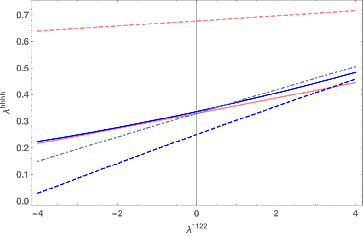
Figure 7: Quartic coupling $\lambda^{hhhh}$ between four light states obtained after integrating out the heavy scalars $H$ and $S$, as a function of $\lambda^{1122}$. Dashed curves show the results obtained at tree level – i.e. $\lambda^{hhhh}=\tilde{\lambda}^{hhhh}$ – in the “perturbative” (light-red) and “non-minimal counterterm” (blue) schemes, while solid and dot-dashed curves are the results at one-loop order in the two schemes – found using equations (7.1) and (7.6). For the values in the “counterterm” scheme, the (blue) solid and dot-dashed curves differ by the choice of couplings used in the one-loop corrections (see eq. (7.6)): the dot-dashed line corresponds to using couplings computed in the standard “perturbative” approach at one loop, and the solid one corresponds to using couplings computed in the modified scheme. The difference between these two choices is formally a two-loop effect.

To compare the different results obtained in the “perturbative” and “non-minimal counterterm” schemes, we consider the parameter points defined – in the non-diagonal basis of eq. (7) – as

$$m_{11}^{2}=(100\ \mathrm{GeV})^{2},\,m_{12}^{2}=(400\ \mathrm{GeV})^{2},\,m_{22}^{2}=(2000\ \mathrm{GeV})^{2},\,m_{S}^{2}=(5000\ \mathrm{GeV})^{2},$$

$$\lambda^{1111}=1,\,\lambda^{1112}=2,\,\lambda^{1122}\in[-4,4],\,\lambda^{1222}=1.5,\,\lambda^{2222}=0.5,$$

$$\lambda^{11SS}=0,\,\lambda^{12SS}=3.5,\,\lambda^{22SS}=0\,.$$ (7.8)

In the above inputs, we have chosen a small value for $m_{12}^{2}$ with respect to $m_{22}^{2}$ in order to have a small mixing between $h$ and $H$ at tree level in the “perturbative” scheme, and we have also taken large values for $m_{S}^{2}$ and $\lambda^{12SS}$ (and thus $\lambda^{hHSS}$) to maximise the effect of the off-diagonal loop-level mixing term proportional to $\overline{\delta}m_{hH}^{2}$ in equation (7.1). Moreover, from the mass parameters in eq. (7.3), we can derive the mass eigenvalues to be $m_{h}=60\ \mathrm{GeV}$ and $m_{H}^{2}=2002\ \mathrm{GeV}$, indeed ensuring that our EFT approach of integrating out the heavy mass eigenstate $H$ and the additional scalar $S$ is valid. We will consider that the input values given in equation (7.3) are defined at renormalisation scale equal to $m_{H}$.

Figure 7 shows the values that we find for $\lambda^{hhhh}$ respectively in the “perturbative” (light-red curves) and the “non-minimal counterterm” (blue curves) schemes, at tree level (dashed lines) and one-loop level (solid lines), as a function of the coupling $\lambda^{1122}$ of the non-diagonal basis. At tree level, one can observe a large difference between the quartic couplings obtained in the two schemes. This can be understood because the mixing between $h$ and $H$ is small at tree level, but the loop-level mixing $\overline{\delta}m^{2}_{hH}$ is large, therefore the relative effect of the loop-induced mixing is large and the mixing angle is modified significantly between the two schemes.

At one-loop, we see that the loop corrections are much larger in the “perturbative” scheme than the “non-minimal counterterm” scheme; again, this comes from the fact that the loop-level mixing term – proportional to $\overline{\delta}m_{hH}^{2}$ – is large for the parameter points we considered. However, while the loop corrections differ in magnitude, the one-loop results for $\lambda^{hhhh}$ in the two approaches are close. The differences that appear for increasing $\lambda^{1122}$ can be interpreted as indications of the importance of two-loop corrections. A simple way to estimate the typical size of the two-loop corrections to the matching is to compute the matching relation (7.6) using for the couplings appearing in the one-loop terms the values obtained in the “perturbative” scheme – i.e. we use equation (7.6) with $\tilde{\lambda}^{hhhh}_{\text{c.t.}}$, $\tilde{\lambda}^{hhHH}$, $\tilde{\lambda}^{hhSS}$, and $\tilde{\lambda}^{hhhH}$ – as the difference with using all couplings computed in the “counterterm” scheme is a two-loop effect. Doing so, we obtain the dot-dashed curve in figure 7, which is still close to the result of the “perturbative masses” scheme and only differs significantly for large $|\lambda^{1122}|$ – this indeed confirms missing two-loop corrections as the origin of the difference between the solid curves for $\lambda^{hhhh}$.

Before ending this section, a final comment is at hand about the choice of inputs and of scheme when integrating out heavy fields. If we had proceeded naively – or incorrectly – and had not specified the scheme in which the diagonal-basis couplings are given, or in which they are computed from other inputs (such as in eq. (7.3)), we could have obtained widely different results for $\lambda^{hhhh}$. Indeed for a given value of $\tilde{\lambda}^{hhhh}$, depending on the scheme that it is considered to be given (or computed) in, the loop corrections that are added to it change drastically – as we saw in the above.

8 Threshold corrections to Yukawa couplings

Finally we discuss threshold corrections to Yukawa couplings, which are much simpler than those to quartic scalar couplings. Since we are not considering heavy gauge bosons, there are no contributions to the matching proportional to gauge couplings (as before, provided we use the same renormalisation scheme both above and below the matching scale). However, we must take mixing effects into account:

$$y^{IJ{{\color[rgb]{0,0,0}p}}}_{EFT}= \ y^{IJ{{\color[rgb]{0,0,0}p}}}_{HET}+\overline{\delta}y^{IJ{{\color[rgb]{0,0,0}p}}}+y^{IJ{{\color[rgb]{0,0,0}\mathcal{R}}}}\delta U_{{{\color[rgb]{0,0,0}\mathcal{R}}}{{\color[rgb]{0,0,0}p}}}-\frac{1}{2}y^{IJ{{\color[rgb]{0,0,0}r}}}\delta Z_{{{\color[rgb]{0,0,0}r}}{{\color[rgb]{0,0,0}p}}}+\bigg{[}y^{I^{\prime}J{{\color[rgb]{0,0,0}p}}}(\delta U_{F})_{I^{\prime}}^{I}+(I\leftrightarrow J)\bigg{]}.$$ (8.1)

Here we use capitals $\{I,J\}$ for fermions (see appendix A for all our conventions). We provide the expressions for $\overline{\delta}y^{IJ{{\color[rgb]{0,0,0}p}}}$ in appendix B.2.2 and $\delta U_{{{\color[rgb]{0,0,0}\mathcal{R}}}{{\color[rgb]{0,0,0}p}}}$ is given either by (3.7) in the “perturbative masses” approach or $0$ in the “counterterm” approach. However, we have so far not discussed fermion mixing, which may be important in models e.g. with heavy top partners, or the FSSM [21, 22]. The derivation is very similar to the scalar case: we give the corrections to the kinetic and mass terms (in two-component spinor notation)

$$\Gamma_{HET}\supset \ i(\delta Z_{F}^{HET})_{J}^{I}\psi_{I}\sigma^{\mu}\partial_{\mu}\overline{\psi}^{J}-\bigg{(}\frac{1}{2}(\delta M^{IJ}+\delta_{ct}M^{IJ})\psi_{I}\psi_{J}+h.c.\bigg{)},$$ (8.2)

in eq. (B.4) (or see [70]), and we can divide the fermions into heavy and light states, then make the identification again $\Delta Z_{F}\equiv\delta Z_{F}^{HET}-\delta Z_{F}^{LET}$ and

$$(\psi_{I})^{HET}\equiv(U_{F})_{I}^{J}(\psi_{J})^{EFT}=(1-\frac{1}{2}\Delta Z_{F}+\delta R_{F})_{I}^{J}\psi_{J}^{EFT}.$$ (8.3)

Here $(\Delta Z_{F})^{\dagger}=\Delta Z_{F},(\delta R_{F})^{\dagger}=-\delta R_{F}$. The difference from scalars is that we should diagonalise the matrix $M_{II^{\prime}}M^{I^{\prime}J}$ (note that Dirac fermions do not have diagonal matrices $M_{IJ}$ in two-spinor notation); if we write $\{L,L^{\prime}\},\{H,H^{\prime},H^{\prime\prime}\}$ as indices for light and heavy fermions respectively, then we have

$$M_{LL}= \ M_{LH}=0,\qquad M_{HH^{\prime\prime}}M^{H^{\prime\prime}H^{\prime}}=\delta_{H}^{H^{\prime}}m_{H}^{2},$$

$$0= -\frac{1}{2}(\Delta Z_{F})_{H}^{L}m_{H}^{2}+(\delta R_{F})_{H}^{L}m_{H}^{2}+(\delta M+\delta_{ct}M)^{LH^{\prime}}M_{H^{\prime}H}$$ (8.4)

which leads to

$$(\delta R_{F})_{H}^{L}= \ \frac{1}{2}(\Delta Z_{F})_{H}^{L}-(\delta M+\delta_{ct}M)^{LH^{\prime}}\frac{M_{H^{\prime}H}}{m_{H}^{2}}$$

$$(\delta U_{F})_{L^{\prime}}^{L}= -\frac{1}{2}(\Delta Z_{F})_{L^{\prime}}^{L}$$

$$(\delta U_{F})_{H}^{L}= \left\{\begin{array}[]{cl}-\delta M^{LH^{\prime}}\frac{M_{H^{\prime}H}}{m_{H}^{2}}&\mathrm{perturbative\ masses\ approach}\\ 0&\mathrm{counterterm\ approach}\end{array}\right..$$ (8.7)

9 Outlook

We have described how to match renormalisable couplings between general theories and explained the different choices that can be made. Our aim is to simplify the calculation of the matching as much as possible, since already at one loop the expressions are rather long; we provide what we expect to be the simplest possible prescription for matching onto the SM using only two-point scalar amplitudes in section 5.1, and the simplest general prescription in equation (4.10).

The logical extension is to pursue our approach(es) at two loops. Beyond one loop, we expect the use of mass counterterms to become more important to simplify the removal of infra-red divergences: in particular, if the hierarchy between $\zeta$ and $M$ is comparable to or greater than one loop order (so that the scales are highly tuned) then we expect the “naive perturbative” approach should break down, because we will not be able to treat the “light” states in the loops as massless. Investigating this and its relationship to the Goldstone Boson Catastrophe [71, 72, 73, 47] will be the subject of future work.

Appendix A Conventions and loop functions

We shall work with a theory of scalars, fermions and massless gauge bosons (i.e. we shall assume for this work that the SM gauge group is not extended). The general Lagrangian interaction terms are

$$\mathcal{L} =\mathcal{L}_{S}+\mathcal{L}_{SF}+\mathcal{L}_{SV}+\mathcal{L}_{FV}+\mathcal{L}_{\rm gauge}+\mathcal{L}_{S\mathrm{ghost}}.$$ (A.1)

We use indices $\{i,j,k,l\}$ for general real scalars, $\{I,J,K,L\}$ for Weyl fermions, and $\{a,b,c,d\}$ for gauge bosons. The interactions are

$$\mathcal{L}_{S} \equiv-\frac{1}{6}a_{ijk}\Phi_{i}\Phi_{j}\Phi_{k}-\frac{1}{24}\tilde{\lambda}_{ijkl}\Phi_{i}\Phi_{j}\Phi_{k}\Phi_{l}$$

$$\mathcal{L}_{SF} \equiv-\frac{1}{2}y^{IJk}\psi_{I}\psi_{J}\Phi_{k}-\frac{1}{2}y_{IJk}\overline{\psi}^{I}\overline{\psi}^{J}\Phi_{k}$$

$$\mathcal{L}_{FV} \equiv g^{aJ}_{I}A_{\mu}^{a}\overline{\psi}^{I}\overline{\sigma}^{\mu}\psi_{J}$$

$$\mathcal{L}_{SV} \equiv\frac{1}{2}g^{abi}A^{a}_{\mu}A^{\mu b}\Phi_{i}+\frac{1}{4}g^{abij}A^{a}_{\mu}A^{\mu b}\Phi_{i}\Phi_{j}+g^{aij}A^{a}_{\mu}\Phi_{i}\partial^{\mu}\Phi_{j}$$

$$\mathcal{L}_{\rm gauge} \equiv g^{abc}A^{a}_{\mu}A^{b}_{\nu}\partial^{\mu}A^{\nu c}-\frac{1}{4}g^{abe}g^{cde}A^{\mu a}A^{\nu b}A_{\mu}^{c}A_{\nu}^{d}+g^{abc}A^{a}_{\mu}c^{b}\partial^{\mu}\overline{c}^{c}$$

$$\mathcal{L}_{S\mathrm{ghost}} \equiv-\frac{1}{2}\xi\hat{g}^{abi}\Phi_{i}\overline{c}^{a}c^{b}.$$ (A.2)

These differ a little from the conventions of e.g. [74] because we use the metric $(+,-,-,-)$. With the assumption that the gauge groups are unbroken, $\mathcal{L}_{S\mathrm{ghost}}=0$. The mass terms of fermions are

$$\mathcal{L}_{F}\supset-\frac{1}{2}M^{IJ}\psi_{I}\psi_{J}-\frac{1}{2}M_{IJ}\overline{\psi}^{I}\overline{\psi}^{J}$$

where $M^{IJ}=M_{IJ}^{*}$ is not necessarily diagonal (indeed it cannot be for Dirac fermions) but

$$M^{IJ}M_{JK}\equiv\delta^{I}_{K}m_{I}^{2}.$$

We will also make use of the effective potential $V_{\text{eff}}$, which we can expand perturbatively to one-loop order as

$$V_{\text{eff}}=V^{(0)}+\kappa V^{(1)}=V^{(0)}+\kappa\big{(}V^{(1)}_{S}+V^{(1)}_{F}+V^{(1)}_{V}\big{)}\,,$$ (A.3)

where $V^{(0)}$ is the tree-level potential, and $V^{(1)}_{S}$, $V^{(1)}_{F}$, $V^{(1)}_{V}$ are respectively the scalar, fermion, and gauge-boson contributions to the one-loop potential, with the loop factor denoted

$$\kappa\equiv\frac{1}{16\pi^{2}}.$$ (A.4)

A.1 One-loop functions

We shall use loop functions that mostly coincide with those of [75]: the one-loop integrals are defined in $d=4-2\epsilon$ dimensions, in terms of Euclidean momenta

$$\mathbf{A}(x) \equiv C\int\frac{d^{d}k}{k^{2}+x}$$ (A.5)

$$\mathbf{B}(p^{2};x,y) \equiv C\int\frac{d^{d}k}{(k^{2}+x)((p-k)^{2}+y)}$$ (A.6)

$$\mathbf{C_{0}}(x,y,z) \equiv C\int\frac{d^{d}k}{(k^{2}+x)(k^{2}+y)(k^{2}+z)}$$ (A.7)

$$\mathbf{D_{0}}(x,y,z,u) \equiv C\int\frac{d^{d}k}{(k^{2}+x)(k^{2}+y)(k^{2}+z)(k^{2}+u)}$$ (A.8)

where

$$C=16\pi^{2}\frac{\mu^{2\epsilon}}{(2\pi)^{d}}\,.$$ (A.9)

We then define

$$Q^{2}\equiv 4\pi e^{-\gamma_{E}}\mu^{2},\qquad\overline{\log}x\equiv\log x/Q^{2}.$$ (A.10)

From these, we use the finite parts, namely

$$A_{0}(x) \equiv\lim_{\epsilon\to 0}\bigg{[}\mathbf{A}(x)+\frac{x}{\epsilon}\bigg{]}=x\big{(}\overline{\log}x-1\big{)}$$

$$B(p^{2};x,y) \equiv\lim_{\epsilon\to 0}\bigg{[}\mathbf{B}(p^{2};x,y)-\frac{1}{\epsilon}\bigg{]}$$

$$P_{SS}(x,y) \equiv-\lim_{\epsilon\to 0}\bigg{[}\mathbf{B}(0;x,y)-\frac{1}{\epsilon}\bigg{]}=\frac{A_{0}(x)-A_{0}(y)}{x-y}=-B(0;x,y)$$

$$P_{SS}(x,x) =\overline{\log}x.$$ (A.11)

The functions $\mathbf{C}_{0},\mathbf{D_{0}}$ are UV-finite, so we can safely take the limit $\epsilon\rightarrow 0$ when there are no IR poles:

$$C_{0}(x,y,z) \equiv\lim_{\epsilon\rightarrow 0}\mathbf{C_{0}}(x,y,z)=\frac{1}{x-y}\bigg{[}P_{SS}(x,z)-P_{SS}(y,z)\bigg{]}$$

$$D_{0}(x,y,z,u) \equiv\lim_{\epsilon\rightarrow 0}\mathbf{D_{0}}(x,y,z,u)=\frac{1}{y-x}\bigg{[}C_{0}(x,z,u)-C_{0}(y,z,u)\bigg{]}.$$ (A.12)

In the case of coincident masses, one can take the limit as $y\rightarrow x$ in the above. Note that $P_{SS},C_{0},D_{0}$ are symmetric under permutation of all masses.

Finally, for the kinetic terms we require the derivatives of the $B$ function evaluated at zero external momentum; we denote throughout with a prime the derivative with respect to external momentum squared:

$$B^{\prime}(0;x,y) \equiv\frac{d}{dp^{2}}B(p^{2};x,y)\bigg{|}_{p^{2}=0}=\frac{1}{2(x-y)^{3}}\bigg{[}x^{2}-y^{2}+2xy\log(y/x)\bigg{]}$$

$$B^{\prime}(0;x,x) =\frac{1}{6x}$$

$$B^{\prime}(0;0,x) =\frac{1}{2x}.$$ (A.13)

A.2 Infra-red safe loop functions

Throughout the text we require infra-red safe loop functions, which can be defined in several ways (as described in section 3.1) but the simplest of which is just using dimensional regularisation. We have

$$\overline{P}_{SS}(0,0) \equiv 0\equiv\overline{C}_{0}(0,0,0)\equiv\overline{D}_{0}(0,0,0,0)$$

$$\overline{C}_{0}(0,0,X) \equiv\frac{1}{X}\overline{P}_{SS}(0,X)=\frac{A_{0}(X)}{X^{2}}$$

$$\overline{D}_{0}(0,0,X,Y) \equiv-\frac{1}{X-Y}\bigg{[}\overline{C}_{0}(0,0,X)-\overline{C}_{0}(0,0,Y)\bigg{]}$$

$$\overline{D}_{0}(0,0,X,X) \equiv\frac{\overline{\log}X-2}{X^{2}}.$$ (A.14)

If we want to retain the infra-red divergences, we have, noting for example that $\mathbf{B}(0;0,0)=0=\frac{1}{\epsilon_{UV}}-\frac{1}{\epsilon_{IR}}+\mathcal{O}(\epsilon)$:

$$P_{SS}(0,0) =\frac{1}{\epsilon_{IR}}$$

$$C_{0}(0,0,0) =D_{0}(0,0,0,0)=0$$

$$C_{0}(0,0,X) =-\frac{1}{X}\frac{1}{\epsilon_{IR}}+\overline{C}_{0}(0,0,X)$$

$$D_{0}(0,0,X,Y) =-\frac{1}{X-Y}\bigg{[}C_{0}(0,0,X)-C_{0}(0,0,Y)\bigg{]}=-\frac{1}{XY}\frac{1}{\epsilon_{IR}}+\overline{D}_{0}(0,0,X,Y)$$

$$D_{0}(0,0,0,X) =\frac{1}{X^{2}}\frac{1}{\epsilon_{IR}}+\overline{D}_{0}(0,0,0,X).$$ (A.15)

Appendix B One-loop threshold corrections

Here we give all of the corrections to all necessary $n$-point functions in the limit of vanishing expectation values and external momenta in a general theory with massless gauge bosons. For the matching procedure we need to compute these in the high-energy theory and use them as described in the body of the paper.

B.1 Two-point couplings

B.1.1 Scalar self-energies

The full expressions for scalar self-energies at one loop were given, for example, in [74]. Here we give the zero-momentum limit:

$$\kappa^{-1}\Pi_{ij}(0)= \ \frac{1}{2}\tilde{\lambda}_{ijxx}A_{0}(m_{x}^{2})+\frac{1}{2}a_{ixy}a_{jxy}P_{SS}(m_{x}^{2},m_{y}^{2})-\xi g^{aik}g^{ajk}A_{0}(m_{k}^{2})$$

$$-\mathrm{Re}[y^{KLi}y_{KLj}]G(0;m_{K}^{2},m_{L}^{2})-2\mathrm{Re}[y^{KLi}y^{K^{\prime}L^{\prime}j}M_{KK^{\prime}}M_{LL^{\prime}}]P_{SS}(m_{K}^{2},m_{L}^{2}),$$

$$\kappa^{-1}\Pi_{ij}^{\prime}(0)= -\frac{1}{2}a_{ixy}a_{jxy}B^{\prime}(0;m^{2}_{x},m^{2}_{y})+g^{aik}g^{ajk}[\frac{1}{2}(\xi+5)-(3-\xi)\overline{\log}m_{k}^{2}]$$

$$-\mathrm{Re}[y^{KLi}y_{KLj}]G^{\prime}(0;m_{K}^{2},m_{L}^{2})+2\mathrm{Re}[y^{KLi}y^{K^{\prime}L^{\prime}j}M_{KK^{\prime}}M_{LL^{\prime}}]B^{\prime}(0;m_{K}^{2},m_{L}^{2}),$$ (B.1)

where

$$G(p^{2};x,y)\equiv \ (p^{2}-x-y)B(p^{2};x,y)+A_{0}(x)+A_{0}(y).$$ (B.2)

We have included the gauge dependent parts, although we do not need them for $\Pi_{ij}^{\prime}$ because they will be the same in both the low- and high-energy theories.

B.1.2 Fermion self-energies

The full expressions for fermion self-energies at one-loop were given, for example, in [70]. Here we simply state the formulae that we need: the zero-momentum and zero gauge coupling limit contributions to the effective action terms

$$\Gamma\supset \ i(\delta Z_{F})_{J}^{I}\psi_{I}\sigma^{\mu}\partial_{\mu}\overline{\psi}^{J}-\bigg{(}\frac{1}{2}\delta M^{IJ}\psi_{I}\psi_{J}+h.c.\bigg{)},$$ (B.3)

and we find

$$(\delta Z_{F})_{J}^{I}|_{g\rightarrow 0} =\kappa y^{IKi}y_{JKi}B_{1}(0;m_{K}^{2},m_{i}^{2}),$$

$$\delta M^{IJ}|_{g\rightarrow 0} =\kappa y^{IKi}y^{JK^{\prime}i}M_{KK^{\prime}}P_{SS}(m_{K}^{2},m_{i}^{2}),$$ (B.4)

where

$$B_{1}(0;x,y)= \ \frac{1}{2}[(x-y)B^{\prime}(0;x,y)-P_{SS}(x,y)].$$ (B.5)

B.1.3 Gauge-boson self-energies

In the absence of heavy gauge bosons, the threshold corrections to gauge boson self-energies come only from fermions and scalars and are given by

$$\Delta\Pi_{ab}(p^{2})= \ \Pi_{ab}^{HET}(p^{2})-\Pi_{ab}^{EFT}(p^{2})=\hat{\Pi}_{ab}^{HET}(p^{2})-\hat{\Pi}_{ab}^{EFT}(p^{2}),$$ (B.6)

$$\kappa^{-1}\hat{\Pi}_{ab}(p^{2})\equiv \ 2g^{aij}g^{bij}\tilde{B}_{22}(p^{2};m_{i}^{2},m_{j}^{2})+2\mathrm{Re}(g^{aI}_{J}g^{bI^{\prime}}_{J^{\prime}}M_{II^{\prime}}M^{JJ^{\prime}})B(p^{2};m_{I}^{2},m_{J}^{2})-g^{aI}_{J}g^{bJ}_{I}H_{0}(p^{2};m_{I}^{2},m_{J}^{2}).$$

The hat indicates that the pure gauge parts have already been removed. The definitions for the functions $H_{0}$ and $\tilde{B}_{22}$ are the same as those of PBMZ [68] and, as they are long, we do not repeat them here. The required limits for the general case are

$$\tilde{B}_{22}(0;m_{i}^{2},m_{j}^{2}) =\frac{1}{4}(m_{i}^{2}-m_{j}^{2})^{2}B^{\prime}(0;m_{i}^{2},m_{j}^{2}).$$

$$H_{0}(0;m_{I}^{2},m_{J}^{2}) =(m_{I}^{2}-m_{J}^{2})^{2}B^{\prime}(0;m_{I}^{2},m_{J}^{2})+(m_{I}^{2}+m_{J}^{2})P_{SS}(m_{I}^{2},m_{J}^{2}).$$ (B.7)

These identities can be used to prove (5.25) at one loop. In the limit of an unbroken gauge group, we have

$$\hat{\Pi}_{ab}(p^{2}) =\kappa g^{2}\delta^{ab}\bigg{[}2S_{2}(i)\tilde{B}_{22}(p^{2};m_{i}^{2},m_{i}^{2})-S_{2}(I)\bigg{(}2m_{I}^{2}B(p^{2};m_{I}^{2},m_{I}^{2})+H_{0}(p^{2};m_{I}^{2},m_{I}^{2})\bigg{)}\bigg{]},$$

$$\hat{\Pi}_{ab}(0) =0\,,$$

$$\hat{\Pi}_{ab}^{\prime}(0) =\kappa g^{2}\delta^{ab}\bigg{[}\frac{1}{6}S_{2}(i)\overline{\log}m_{i}^{2}+\frac{2}{3}S_{2}(I)\overline{\log}m_{I}^{2}\bigg{]},$$ (B.8)

where $S_{2}$ is the Dynkin index of the representation of the scalars or fermions, and $g$ is the gauge coupling for the unbroken gauge group. The final expression gives the well-known one-loop corrections to gauge thresholds:

$$g_{EFT}^{2}\delta_{ab}=g^{2}_{HET}\delta_{ab}+g^{2}\bigg{[}(\hat{\Pi}^{\prime}_{ab}(0))^{HET}-(\hat{\Pi}^{\prime}_{ab}(0))^{EFT}\bigg{]}.$$ (B.9)

B.2 Three-point couplings

The only relevant three-point couplings that we need are cubic scalar couplings and Yukawa couplings, all those involving gauge bosons just being given by the gauge couplings.

B.2.1 Scalar couplings

For a term in the effective action

$$\Gamma\supset-\frac{1}{6}\delta a_{ijk}\Phi_{i}\Phi_{j}\Phi_{k}$$ (B.10)

recall that we have

$$\delta a_{ijk}=\kappa\frac{\partial^{3}V^{(1)}}{\partial\Phi_{i}\partial\Phi_{j}\partial\Phi_{k}},\qquad V^{(1)}\equiv V^{(1)}_{S}+V^{(1)}_{F}+V^{(1)}_{V}.$$ (B.11)

Then

$$\frac{\partial^{3}V^{(1)}_{S}}{\partial\Phi_{i}\partial\Phi_{j}\partial\Phi_{k}}= \ \frac{1}{4}\tilde{\lambda}_{ijxy}a_{kxy}P_{SS}(m_{x}^{2},m_{y}^{2})+\frac{1}{6}a_{kxy}a_{jyz}a_{izx}C_{0}(m_{x}^{2},m_{y}^{2},m_{z}^{2})+(ijk)\,,$$ (B.12)

$$\frac{\partial^{3}V^{(1)}_{F}}{\partial\Phi_{i}\partial\Phi_{j}\partial\Phi_{k}}= -\frac{2}{3}\mathrm{Re}(y^{IJi}y^{J^{\prime}Kj}y^{K^{\prime}I^{\prime}k}M_{II^{\prime}}M_{JJ^{\prime}}M_{KK^{\prime}})C_{0}(m_{I}^{2},m_{J}^{2},m_{K}^{2})$$

$$-2\mathrm{Re}(y^{IJi}y^{J^{\prime}Kj}y_{KIk}M_{JJ^{\prime}})F_{3}(m_{I}^{2},m_{J}^{2},m_{K}^{2})+(ijk)\,,$$ (B.13)

where

$$F_{3}(m_{I}^{2},m_{J}^{2},m_{K}^{2})\equiv \lim_{\epsilon\to 0}\bigg{[}C\int d^{d}k(-k^{2})\left(\prod_{\mathcal{I}\in\{I,J,K\}}\frac{1}{k^{2}+m_{\mathcal{I}}^{2}}\right)+\frac{1}{\epsilon}\bigg{]}$$

$$= \ m_{I}^{2}C_{0}(m_{I}^{2},m_{J}^{2},m_{K}^{2})+P_{SS}(m_{J}^{2},m_{K}^{2}).$$ (B.14)

Note that the function $F_{3}$ could also have been written in a form where it is manifestly symmetric under the exchange of any two of its arguments. It only has an infra-red divergence for all three arguments vanishing, so we can define

$$\overline{F}_{3}(0,0,0)=0;\qquad\overline{F}_{3}(x,y,z)=F_{3}(x,y,z)\qquad(x,y,z)\neq(0,0,0).$$ (B.15)

Finally for contributions from massless gauge bosons:

$$\frac{\partial^{3}V^{(1)}_{V}}{\partial\Phi_{i}\partial\Phi_{j}\partial\Phi_{k}} =-\frac{1}{2}\xi g^{ail}g^{ajm}a_{lmk}P_{SS}(m_{l}^{2},m_{m}^{2})+(ijk)+\mathcal{O}(g^{3}).$$ (B.16)

The $\mathcal{O}(g^{3})$ pieces automatically cancel between high- and low-energy theories, so we do not include them.

B.2.2 Yukawa couplings

With our assumptions of having no heavy gauge bosons, the only vertex corrections to Yukawa couplings come from triangle diagrams with scalars and fermions in the loop. The result is that

$$\Gamma\supset -\frac{1}{2}\delta y^{IJi}\psi_{I}\psi_{J}\Phi_{i},$$

$$\kappa^{-1}\overline{\delta}y^{IJi}= \ M_{KK^{\prime}}a_{ijk}y^{KIk}y^{K^{\prime}Jj}C_{0}(m_{j}^{2},m_{k}^{2},m_{K}^{2})-y^{KIk}y^{K^{\prime}Jk}y_{KK^{\prime}i}\overline{F}_{3}(m_{k}^{2},m_{K}^{2},m_{K^{\prime}}^{2})$$

$$+M_{KL}M_{K^{\prime}L^{\prime}}y^{LL^{\prime}i}y^{KIk}y^{K^{\prime}Jk}C_{0}(m_{k}^{2},m_{K}^{2},m_{K^{\prime}}^{2}).$$ (B.17)

To find the matching condition, we need to supplement this with corrections from the scalar and fermion self-energies and insert them all in equation (8.1). Note that the infra-red divergences are much more simply tamed than in the pure scalar couplings: the difference between the HET and EFT is automatically infra-red safe and corresponds just to replacing $F_{3}\rightarrow\overline{F}_{3}$ in the HET. The other two terms are always infra-red safe, because the first term can only diverge for the case of $j,k$ both light fields, so the coupling $a^{ijk}$ must vanish when $i$ is also light; while the last term has mass prefactors that vanish for light fermions.

B.3 Four-point couplings

For a term in the effective action

$$\Gamma\supset-\frac{1}{24}\delta\tilde{\lambda}_{ijkl}\Phi_{i}\Phi_{j}\Phi_{k}\Phi_{l}$$ (B.18)

recall that we have

$$\delta\tilde{\lambda}_{ijkl}=\kappa\frac{\partial^{4}V^{(1)}}{\partial\Phi_{i}\partial\Phi_{j}\partial\Phi_{k}\partial\Phi_{l}},\qquad V^{(1)}\equiv V^{(1)}_{S}+V^{(1)}_{F}+V^{(1)}_{V}.$$ (B.19)

Then

$$\frac{\partial^{4}V^{(1)}_{S}}{\partial\Phi_{i}\partial\Phi_{j}\partial\Phi_{k}\partial\Phi_{l}}= \ \frac{1}{16}\tilde{\lambda}_{ijxy}\tilde{\lambda}_{klxy}P_{SS}(m_{x}^{2},m_{y}^{2})+\frac{1}{4}\tilde{\lambda}_{ijxy}a_{kyz}a_{lzx}C_{0}(m_{x}^{2},m_{y}^{2},m_{z}^{2})$$

$$-\frac{1}{8}a_{ixy}a_{jyz}a_{kzu}a_{lux}D_{0}(m_{x}^{2},m_{y}^{2},m_{z}^{2},m_{u}^{2})+(ijkl).$$ (B.20)

$$\frac{\partial^{4}V^{(1)}_{F}}{\partial\Phi_{i}\partial\Phi_{j}\partial\Phi_{k}\partial\Phi_{l}}= \ \frac{1}{2}\mathrm{Re}(y^{IJi}y^{J^{\prime}Kj}y^{K^{\prime}Lk}y^{L^{\prime}I^{\prime}l}M_{II^{\prime}}M_{JJ^{\prime}}M_{KK^{\prime}}M_{LL^{\prime}})D_{0}(m_{I}^{2},m_{J}^{2},m_{K}^{2},m_{L}^{2})$$

$$+2\mathrm{Re}(y^{IJi}y^{J^{\prime}Kj}y^{K^{\prime}Lk}y_{LIl}M_{JJ^{\prime}}M_{KK^{\prime}})F_{4}(m_{I}^{2},m_{J}^{2},m_{K}^{2},m_{L}^{2})$$

$$+\mathrm{Re}(y^{IJi}y^{J^{\prime}Kj}y_{KLk}y_{L^{\prime}Il}M_{JJ^{\prime}}M^{LL^{\prime}})F_{4}(m_{I}^{2},m_{J}^{2},m_{K}^{2},m_{L}^{2})$$

$$+\frac{1}{2}\mathrm{Re}(y^{IJi}y_{JKj}y^{KLk}y_{LIl})H_{4}(m_{I}^{2},m_{J}^{2},m_{K}^{2},m_{L}^{2})+(ijkl)\,,$$ (B.21)

where $F_{4}$ and $H_{4}$ are defined in terms of Euclidean momenta as

$$F_{4}(m_{I}^{2},m_{J}^{2},m_{K}^{2},m_{L}^{2})\equiv \ \lim_{\epsilon\rightarrow 0}C\int d^{d}k(-k^{2})\left(\prod_{\mathcal{I}\in\{I,J,K,L\}}\frac{1}{k^{2}+m_{\mathcal{I}}^{2}}\right)$$

$$= \ m_{I}^{2}D_{0}(m_{I}^{2},m_{J}^{2},m_{K}^{2},m_{L}^{2})-C_{0}(m_{J}^{2},m_{K}^{2},m_{L}^{2})$$

$$H_{4}(m_{I}^{2},m_{J}^{2},m_{K}^{2},m_{L}^{2})\equiv \ \lim_{\epsilon\rightarrow 0}\bigg{[}C\int d^{d}k(k^{4})\left(\prod_{\mathcal{I}\in\{I,J,K,L\}}\frac{1}{k^{2}+m_{\mathcal{I}}^{2}}\right)-\frac{1}{\epsilon}\bigg{]}$$

$$= -P_{SS}(m_{K}^{2},m_{L}^{2})+\big{(}m_{I}^{2}+m_{J}^{2}\big{)}F_{4}(m_{I}^{2},m_{J}^{2},m_{K}^{2},m_{L}^{2})$$

$$-m_{I}^{2}m_{J}^{2}D_{0}(m_{I}^{2},m_{J}^{2},m_{K}^{2},m_{L}^{2})\,,$$

and, as before, $(ijkl)$ denotes the 24 possible permutations of $\{i,j,k,l\}$. Note that to pass to infra-red safe expressions we replace $P_{SS},C_{0},D_{0}$ by $\overline{P}_{SS},\overline{C}_{0},\overline{D}_{0}$ in the above.

Finally the contributions from massless gauge bosons are:

$$\frac{\partial^{4}V^{(1)}_{V}}{\partial\Phi_{i}\partial\Phi_{j}\partial\Phi_{k}\partial\Phi_{l}}\bigg{|}_{\mathcal{O}(g^{2})}= -\frac{1}{4}\xi g^{aim}g^{ajn}\tilde{\lambda}_{mnkl}P_{SS}(m_{m}^{2},m_{n}^{2})$$

$$-\frac{1}{2}\xi g^{aim}g^{ajr}a_{mnk}a_{nrl}C_{0}(m_{m}^{2},m_{n}^{2},m_{r}^{2})+(ijkl).$$ (B.22)

We omit the terms of higher order in the gauge coupling, which automatically cancel between high- and low-energy theories except when they are given in different schemes.

Appendix C Cancellation of infra-red divergences

In this appendix we explicitly show the cancellation of infra-red divergences in the matching of quartic scalar couplings. We start by considering the case of purely scalar contributions to the different terms in the matching, before turning to the case of fermionic contributions in appendix C.1. We have already demonstrated the complete cancellation of contributions from gauge interactions in section 3.3.

For the diagrams with only scalars in the loops, let us first summarise the infra-red divergent parts of the necessary quantities in the high-energy theory:

$$\kappa^{-1}\delta m_{{{\color[rgb]{0,0,0}\mathcal{P}}}{{\color[rgb]{0,0,0}\mathcal{Q}}}}^{2}= \ \frac{1}{2}a_{{{\color[rgb]{0,0,0}\mathcal{P}}}{{\color[rgb]{0,0,0}x}}{{\color[rgb]{0,0,0}y}}}a_{{{\color[rgb]{0,0,0}\mathcal{Q}}}{{\color[rgb]{0,0,0}x}}{{\color[rgb]{0,0,0}y}}}P_{SS}(m_{{\color[rgb]{0,0,0}x}}^{2},m_{{\color[rgb]{0,0,0}y}}^{2})+\mathrm{IR\ safe},$$

$$\kappa^{-1}\delta a_{{{\color[rgb]{0,0,0}\mathcal{P}}}{{\color[rgb]{0,0,0}q}}{{\color[rgb]{0,0,0}r}}}= \ \frac{1}{2}a_{{{\color[rgb]{0,0,0}\mathcal{P}}}{{\color[rgb]{0,0,0}x}}{{\color[rgb]{0,0,0}y}}}a_{{{\color[rgb]{0,0,0}q}}{{\color[rgb]{0,0,0}y}}{{\color[rgb]{0,0,0}\mathcal{Q}}}}a_{{{\color[rgb]{0,0,0}r}}{{\color[rgb]{0,0,0}\mathcal{Q}}}{{\color[rgb]{0,0,0}x}}}C_{0}(m_{{\color[rgb]{0,0,0}x}}^{2},m_{{\color[rgb]{0,0,0}y}}^{2},m_{{\color[rgb]{0,0,0}\mathcal{Q}}}^{2})+\frac{1}{4}\tilde{\lambda}_{{{\color[rgb]{0,0,0}q}}{{\color[rgb]{0,0,0}r}}{{\color[rgb]{0,0,0}x}}{{\color[rgb]{0,0,0}y}}}a_{{{\color[rgb]{0,0,0}\mathcal{P}}}{{\color[rgb]{0,0,0}x}}{{\color[rgb]{0,0,0}y}}}P_{SS}(m_{{\color[rgb]{0,0,0}x}}^{2},m_{{\color[rgb]{0,0,0}y}}^{2})+({{\color[rgb]{0,0,0}q}}\leftrightarrow{{\color[rgb]{0,0,0}r}})+\mathrm{IR\ safe},$$ (C.1)

$$\kappa^{-1}\delta\tilde{\lambda}_{{{\color[rgb]{0,0,0}p}}{{\color[rgb]{0,0,0}q}}{{\color[rgb]{0,0,0}r}}{{\color[rgb]{0,0,0}s}}}= \ \frac{1}{16}\tilde{\lambda}_{{{\color[rgb]{0,0,0}p}}{{\color[rgb]{0,0,0}q}}{{\color[rgb]{0,0,0}x}}{{\color[rgb]{0,0,0}y}}}\tilde{\lambda}_{{{\color[rgb]{0,0,0}r}}{{\color[rgb]{0,0,0}s}}{{\color[rgb]{0,0,0}x}}{{\color[rgb]{0,0,0}y}}}P_{SS}(m_{{\color[rgb]{0,0,0}x}}^{2},m_{{\color[rgb]{0,0,0}y}}^{2})+\frac{1}{4}\tilde{\lambda}_{{{\color[rgb]{0,0,0}p}}{{\color[rgb]{0,0,0}q}}{{\color[rgb]{0,0,0}x}}{{\color[rgb]{0,0,0}y}}}a_{{{\color[rgb]{0,0,0}r}}{{\color[rgb]{0,0,0}y}}{{\color[rgb]{0,0,0}\mathcal{Q}}}}a_{{{\color[rgb]{0,0,0}s}}{{\color[rgb]{0,0,0}\mathcal{Q}}}{{\color[rgb]{0,0,0}x}}}C_{0}(m_{{\color[rgb]{0,0,0}x}}^{2},m_{{\color[rgb]{0,0,0}y}}^{2},m_{{\color[rgb]{0,0,0}\mathcal{Q}}}^{2})$$

$$-\frac{1}{4}a_{{{\color[rgb]{0,0,0}p}}{{\color[rgb]{0,0,0}x}}{{\color[rgb]{0,0,0}\mathcal{Q}}}}a_{{{\color[rgb]{0,0,0}q}}{{\color[rgb]{0,0,0}\mathcal{Q}}}{{\color[rgb]{0,0,0}z}}}a_{{{\color[rgb]{0,0,0}r}}{{\color[rgb]{0,0,0}z}}{{\color[rgb]{0,0,0}\mathcal{R}}}}a_{{{\color[rgb]{0,0,0}s}}{{\color[rgb]{0,0,0}\mathcal{R}}}{{\color[rgb]{0,0,0}x}}}D_{0}(m_{{\color[rgb]{0,0,0}x}}^{2},m_{{\color[rgb]{0,0,0}\mathcal{Q}}}^{2},m_{{\color[rgb]{0,0,0}z}}^{2},m_{{\color[rgb]{0,0,0}\mathcal{R}}}^{2})+({{\color[rgb]{0,0,0}p}}{{\color[rgb]{0,0,0}q}}{{\color[rgb]{0,0,0}r}}{{\color[rgb]{0,0,0}s}})+\mathrm{IR\ safe}.$$

These must cancel against the calculation of $\delta\lambda_{{{\color[rgb]{0,0,0}p}}{{\color[rgb]{0,0,0}q}}{{\color[rgb]{0,0,0}r}}{{\color[rgb]{0,0,0}s}}}$ in the low-energy theory:

$$\kappa^{-1}\delta\lambda_{{{\color[rgb]{0,0,0}p}}{{\color[rgb]{0,0,0}q}}{{\color[rgb]{0,0,0}r}}{{\color[rgb]{0,0,0}s}}}= \ \frac{1}{16}P_{SS}(m_{{\color[rgb]{0,0,0}x}}^{2},m_{{\color[rgb]{0,0,0}y}}^{2})\lambda_{{{\color[rgb]{0,0,0}p}}{{\color[rgb]{0,0,0}q}}{{\color[rgb]{0,0,0}x}}{{\color[rgb]{0,0,0}y}}}\lambda_{{{\color[rgb]{0,0,0}r}}{{\color[rgb]{0,0,0}s}}{{\color[rgb]{0,0,0}x}}{{\color[rgb]{0,0,0}y}}}+({{\color[rgb]{0,0,0}p}}{{\color[rgb]{0,0,0}q}}{{\color[rgb]{0,0,0}r}}{{\color[rgb]{0,0,0}s}})$$ (C.2)

$$= \ \frac{1}{16}P_{SS}(m_{{\color[rgb]{0,0,0}x}}^{2},m_{{\color[rgb]{0,0,0}y}}^{2})\bigg{[}\tilde{\lambda}_{{{\color[rgb]{0,0,0}p}}{{\color[rgb]{0,0,0}q}}{{\color[rgb]{0,0,0}x}}{{\color[rgb]{0,0,0}y}}}\tilde{\lambda}_{{{\color[rgb]{0,0,0}r}}{{\color[rgb]{0,0,0}s}}{{\color[rgb]{0,0,0}x}}{{\color[rgb]{0,0,0}y}}}-\frac{2}{m_{{\color[rgb]{0,0,0}\mathcal{P}}}^{2}}(a_{{{\color[rgb]{0,0,0}\mathcal{P}}}{{\color[rgb]{0,0,0}p}}{{\color[rgb]{0,0,0}q}}}a_{{{\color[rgb]{0,0,0}\mathcal{P}}}{{\color[rgb]{0,0,0}x}}{{\color[rgb]{0,0,0}y}}}+2a_{{{\color[rgb]{0,0,0}\mathcal{P}}}{{\color[rgb]{0,0,0}p}}{{\color[rgb]{0,0,0}x}}}a_{{{\color[rgb]{0,0,0}\mathcal{P}}}{{\color[rgb]{0,0,0}q}}{{\color[rgb]{0,0,0}y}}})\tilde{\lambda}_{{{\color[rgb]{0,0,0}r}}{{\color[rgb]{0,0,0}s}}{{\color[rgb]{0,0,0}x}}{{\color[rgb]{0,0,0}y}}}$$

$$\ \ +\frac{1}{m_{{\color[rgb]{0,0,0}\mathcal{P}}}^{2}m_{{\color[rgb]{0,0,0}\mathcal{Q}}}^{2}}\bigg{(}a_{{{\color[rgb]{0,0,0}\mathcal{P}}}{{\color[rgb]{0,0,0}p}}{{\color[rgb]{0,0,0}q}}}a_{{{\color[rgb]{0,0,0}\mathcal{Q}}}{{\color[rgb]{0,0,0}r}}{{\color[rgb]{0,0,0}s}}}a_{{{\color[rgb]{0,0,0}\mathcal{P}}}{{\color[rgb]{0,0,0}x}}{{\color[rgb]{0,0,0}y}}}a_{{{\color[rgb]{0,0,0}\mathcal{Q}}}{{\color[rgb]{0,0,0}x}}{{\color[rgb]{0,0,0}y}}}+4a_{{{\color[rgb]{0,0,0}\mathcal{P}}}{{\color[rgb]{0,0,0}p}}{{\color[rgb]{0,0,0}q}}}a_{{{\color[rgb]{0,0,0}\mathcal{P}}}{{\color[rgb]{0,0,0}x}}{{\color[rgb]{0,0,0}y}}}a_{{{\color[rgb]{0,0,0}\mathcal{Q}}}{{\color[rgb]{0,0,0}r}}{{\color[rgb]{0,0,0}x}}}a_{{{\color[rgb]{0,0,0}\mathcal{Q}}}{{\color[rgb]{0,0,0}s}}{{\color[rgb]{0,0,0}y}}}+4a_{{{\color[rgb]{0,0,0}\mathcal{P}}}{{\color[rgb]{0,0,0}p}}{{\color[rgb]{0,0,0}x}}}a_{{{\color[rgb]{0,0,0}\mathcal{P}}}{{\color[rgb]{0,0,0}q}}{{\color[rgb]{0,0,0}y}}}a_{{{\color[rgb]{0,0,0}\mathcal{Q}}}{{\color[rgb]{0,0,0}r}}{{\color[rgb]{0,0,0}x}}}a_{{{\color[rgb]{0,0,0}\mathcal{Q}}}{{\color[rgb]{0,0,0}s}}{{\color[rgb]{0,0,0}y}}}\bigg{)}\bigg{]}+({{\color[rgb]{0,0,0}p}}{{\color[rgb]{0,0,0}q}}{{\color[rgb]{0,0,0}r}}{{\color[rgb]{0,0,0}s}}).$$

Collecting these together in the matching relation for the scalar quartic coupling, equation (3.2), one finds for the potentially divergent terms:

$$\kappa^{-1}\Delta\lambda_{{{\color[rgb]{0,0,0}p}}{{\color[rgb]{0,0,0}q}}{{\color[rgb]{0,0,0}r}}{{\color[rgb]{0,0,0}s}}}\supset \ \frac{1}{4}\tilde{\lambda}_{{{\color[rgb]{0,0,0}r}}{{\color[rgb]{0,0,0}s}}{{\color[rgb]{0,0,0}x}}{{\color[rgb]{0,0,0}y}}}a_{{{\color[rgb]{0,0,0}\mathcal{P}}}{{\color[rgb]{0,0,0}p}}{{\color[rgb]{0,0,0}x}}}a_{{{\color[rgb]{0,0,0}\mathcal{P}}}{{\color[rgb]{0,0,0}q}}{{\color[rgb]{0,0,0}y}}}\bigg{[}C_{0}(m_{{\color[rgb]{0,0,0}x}}^{2},m_{{\color[rgb]{0,0,0}y}}^{2},m_{{\color[rgb]{0,0,0}\mathcal{P}}}^{2})+\frac{1}{m_{{\color[rgb]{0,0,0}\mathcal{P}}}^{2}}P_{SS}(m_{{\color[rgb]{0,0,0}x}}^{2},m_{{\color[rgb]{0,0,0}y}}^{2})\bigg{]}$$

$$-\frac{1}{4}a_{{{\color[rgb]{0,0,0}\mathcal{P}}}{{\color[rgb]{0,0,0}p}}{{\color[rgb]{0,0,0}x}}}a_{{{\color[rgb]{0,0,0}\mathcal{P}}}{{\color[rgb]{0,0,0}q}}{{\color[rgb]{0,0,0}y}}}a_{{{\color[rgb]{0,0,0}\mathcal{Q}}}{{\color[rgb]{0,0,0}r}}{{\color[rgb]{0,0,0}x}}}a_{{{\color[rgb]{0,0,0}\mathcal{Q}}}{{\color[rgb]{0,0,0}s}}{{\color[rgb]{0,0,0}y}}}\frac{1}{m_{{\color[rgb]{0,0,0}\mathcal{P}}}^{2}}\bigg{[}C_{0}(m_{{\color[rgb]{0,0,0}x}}^{2},m_{{\color[rgb]{0,0,0}y}}^{2},m_{{\color[rgb]{0,0,0}\mathcal{Q}}}^{2})+\frac{1}{m_{{\color[rgb]{0,0,0}\mathcal{Q}}}^{2}}P_{SS}(m_{{\color[rgb]{0,0,0}x}}^{2},m_{{\color[rgb]{0,0,0}y}}^{2})\bigg{]}$$

$$-\frac{1}{4}a_{{{\color[rgb]{0,0,0}\mathcal{P}}}{{\color[rgb]{0,0,0}p}}{{\color[rgb]{0,0,0}x}}}a_{{{\color[rgb]{0,0,0}\mathcal{P}}}{{\color[rgb]{0,0,0}q}}{{\color[rgb]{0,0,0}y}}}a_{{{\color[rgb]{0,0,0}\mathcal{Q}}}{{\color[rgb]{0,0,0}r}}{{\color[rgb]{0,0,0}x}}}a_{{{\color[rgb]{0,0,0}\mathcal{Q}}}{{\color[rgb]{0,0,0}s}}{{\color[rgb]{0,0,0}y}}}\bigg{[}D_{0}(m_{{\color[rgb]{0,0,0}x}}^{2},m_{{\color[rgb]{0,0,0}\mathcal{P}}}^{2},m_{{\color[rgb]{0,0,0}y}}^{2},m_{{\color[rgb]{0,0,0}\mathcal{Q}}}^{2})+\frac{1}{m_{{\color[rgb]{0,0,0}\mathcal{P}}}^{2}m_{{\color[rgb]{0,0,0}\mathcal{Q}}}^{2}}P_{SS}(m_{{\color[rgb]{0,0,0}x}}^{2},m_{{\color[rgb]{0,0,0}y}}^{2})\bigg{]}+({{\color[rgb]{0,0,0}p}}{{\color[rgb]{0,0,0}q}}{{\color[rgb]{0,0,0}r}}{{\color[rgb]{0,0,0}s}})$$ (C.3)

The terms in square brackets are all finite as we take the limit $m_{{\color[rgb]{0,0,0}x}},m_{{\color[rgb]{0,0,0}y}}\rightarrow 0$, and could be taken as the definitions of the functions $\overline{C}_{0}(0,0,X),\overline{D}_{0}(0,0,X,Y)$ which agree with our dimensional-regularisation definitions (A.14). Note that these do not give the limiting expressions for $\overline{C}_{0}(0,0,0),\overline{D}_{0}(0,0,0,0)$ which, as mentioned in section 3.1, remain ambiguous but give no net contribution when we subtract the contribution of the LET from that of the HET in the matching.

C.1 Absence of IR divergences from massless fermions

We can now show that vanishing fermion masses cause no divergence in the fermion contributions to the matching of three- and four-point functions – see eqs. (B.13) and (B.3). First of all, it should be noted that terms in which all the fermion masses vanish do not pose a problem in the matching because they appear in both the high- and low-energy parts of the matching.

Then, considering the three-point contribution in eq. (B.13), one can notice immediately that the first term – of the form $M_{II^{\prime}}M_{JJ^{\prime}}M_{KK^{\prime}}C_{0}(m_{I}^{2},m_{J}^{2},m_{K}^{2})$ – cannot be divergent, because by itself the function $C_{0}$ diverges at most as an inverse mass-squared if all its three arguments tend to 0 – recall that $C_{0}(\delta,\delta,\delta)=1/2\delta$. For the second term, in the case where $M_{JJ^{\prime}}$ vanishes, the overall term is also zero, however there remains to verify that $F_{3}(m_{I}^{2},m_{J}^{2},m_{K}^{2})$ is regular in the limit where $m_{I}^{2}$ and $m_{K}^{2}$ go to zero (if only one of these two masses is zero, the $P_{SS}$ and $C_{0}$ functions are not divergent). We have then

$$F_{3}(\delta,m_{J}^{2},\delta)= \ \delta C_{0}(\delta,m_{J}^{2},\delta)+P_{SS}(m_{J}^{2},\delta)\underset{\mathclap{\delta\to 0}}{\longrightarrow}\frac{A_{0}(m_{J}^{2})}{m_{J}^{2}}\,,$$ (C.4)

as we know that $C_{0}(\delta,\delta,m_{J}^{2})$ diverges as $\log\delta$.

Turning now to the four-point couplings, for which the fermion contribution is given in equation (B.3), we have three types of terms to verify. First, the term $M_{II^{\prime}}M_{JJ^{\prime}}M_{KK^{\prime}}M_{LL^{\prime}}D_{0}(m_{I}^{2},m_{J}^{2},m_{K}^{2},m_{L}^{2})$ is not divergent even if all four mass arguments are zero because $D_{0}(\delta,\delta,\delta,\delta)=1/6\delta^{2}$. Second, we must consider the terms involving the function $F_{4}(m_{I}^{2},m_{J}^{2},m_{K}^{2},m_{L}^{2})$: if three (or four) of the masses are zero, the mass prefactors ensure that the contributions to the four-point coupling are not divergent. However, it is necessary to verify what happens when only two mass arguments vanish, say $m_{I}^{2}$ and $m_{J}^{2}$. We find

$$F_{4}(\delta,\delta,m_{K}^{2},m_{L}^{2})= \ \delta D_{0}(\delta,\delta,m_{K}^{2},m_{L}^{2})-C_{0}(\delta,m_{K}^{2},m_{L}^{2})$$

$$\underset{\delta\to 0}{\to} -C_{0}(0,m_{K}^{2},m_{L}^{2})\,,$$ (C.5)

as $D_{0}(\delta,\delta,m_{K}^{2},m_{L}^{2})$ diverges like $\log\delta$.

There remains to show that $H_{4}(m_{I}^{2},m_{J}^{2},m_{K}^{2},m_{L}^{2})$ is not divergent when one or several of its arguments are zero. For only one vanishing mass, this is apparent from its definition in eq. (B.3). Then, we can consider the case of two vanishing masses, say $m_{I}^{2}$ and $m_{J}^{2}$:

$$H_{4}(\delta,\delta,m_{K}^{2},m_{L}^{2})= -P_{SS}(m_{K}^{2},m_{L}^{2})+2\delta F_{4}(\delta,\delta,m_{K}^{2},m_{L}^{2})-\delta^{2}D_{0}(\delta,\delta,m_{K}^{2},m_{L}^{2})$$

$$\underset{\mathclap{\delta\to 0}}{\longrightarrow} -P_{SS}(m_{K}^{2},m_{L}^{2})$$ (C.6)

The case with three zero masses is also simple to verify, requiring only the intermediate results

$$D_{0}(\delta,\delta,\delta,m_{L}^{2}) \underset{\delta\to 0}{\to}\frac{1}{2m_{L}^{2}\delta}+\frac{\overline{\log}\delta}{m_{L}^{4}}-\frac{A_{0}(m_{L}^{2})}{m_{L}^{6}}+\frac{1}{2m_{L}^{4}}$$ (C.7)

$$F_{4}(\delta,\delta,\delta,m_{L}^{2}) \underset{\delta\to 0}{\to}\frac{\overline{\log}\delta}{m_{L}^{2}}-\frac{A_{0}(m_{L}^{2})}{m_{L}^{4}}+\frac{1}{2m_{L}^{2}}$$ (C.8)

and we find

$$H_{4}(\delta,\delta,\delta,m_{L}^{2})= -P_{SS}(\delta,m_{L}^{2})+2\delta F_{4}(\delta,\delta,\delta,m_{L}^{2})-\delta^{2}D_{0}(\delta,\delta,\delta,m_{L}^{2})\underset{\mathclap{\delta\to 0}}{\longrightarrow}-\frac{A_{0}(m_{L}^{2})}{m_{L}^{2}}$$ (C.9)

Finally, if all four of its mass arguments are zero, the function $H_{4}(\delta,\delta,\delta,\delta)$ does diverge, but this does not cause a problem for the matching because a term with all fermion masses vanishing would appear both in the EFT and the UV-complete sides of the matching condition.

Appendix D Threshold corrections to the electroweak gauge couplings

We present in this appendix details about the derivation of the threshold corrections to $g_{Y}$ and $g_{2}$ – the gauge couplings of $U(1)_{Y}$ and $SU(2)_{L}$ , respectively – given in equation (5.5). The radiative corrections to gauge couplings are obtained as the corrections to the gauge-boson kinetic term, i.e.

$$\frac{1}{4g^{2}}F_{\mu\nu}F^{\mu\nu}\longrightarrow\frac{1}{4g^{2}}\left(1+\Delta Z_{A}\right)F_{\mu\nu}F^{\mu\nu},$$ (D.1)

where $A_{\mu}$ is the gauge boson of some gauge group, $F_{\mu\nu}$ the associated field-strength tensor, and $g$ the gauge coupling. In the above relation we have $\Delta Z_{A}=-\Pi_{AA}^{\prime}(0)$, the latter being the derivative with respect to external momentum of the transverse part of the gauge-boson self-energy. Applying this to $U(1)_{Y}$, the threshold correction to $g_{Y}$ is found with the relation

$$\frac{1}{4g_{Y}^{2}}\left(1-\Pi_{BB}^{HET\,\prime}(0)\right)B_{\mu\nu}B^{\mu\nu}=\frac{1}{4(g_{Y}^{2}+\Delta_{g_{Y}^{2}})}\left(1-\Pi_{BB}^{SM\,\prime}(0)\right)B_{\mu\nu}B^{\mu\nu},$$ (D.2)

where $B_{\mu}$ is the gauge boson of $U(1)_{Y}$ and $B_{\mu\nu}$ the corresponding field-strength, and the self-energies on the left and on the right are computed in the high-energy theory and in the SM, respectively. We thus obtain

$$\Delta_{g_{Y}^{2}}=g_{Y}^{2}\left[\Pi_{BB}^{HET\,\prime}(0)-\Pi_{BB}^{SM\,\prime}(0)\right].$$ (D.3)

Similarly, for $SU(2)_{L}$, we obtain

$$\Delta_{g_{2}^{2}}=g_{2}^{2}\left[\Pi_{W_{3}W_{3}}^{HET\,\prime}(0)-\Pi_{W_{3}W_{3}}^{SM\,\prime}(0)\right],$$ (D.4)

where $W_{3}$ is the third component of the $SU(2)_{L}$ gauge boson. Now, expressing the $Z$-boson mass eigenstate in terms of $W_{3}$ and $B$, we have

$$(g_{Y}^{2}+g_{2}^{2})\Pi_{ZZ}=g_{2}^{2}\Pi_{W_{3}W_{3}}-2g_{Y}g_{2}\Pi_{W_{3}B}+g_{Y}^{2}\Pi_{BB}.$$ (D.5)

Finally, as we need in section 5 the gauge threshold corrections in the limit $v\to 0$, we know from gauge invariance that in this limit the $\Pi_{W_{3}B}$ term should vanish. Taking all these intermediate results together, we obtain

$$\Delta_{g_{Y}^{2}}+\Delta_{g_{2}^{2}}\Big{|}_{v=0}=(g_{Y}^{2}+g_{2}^{2})\bigg{[}\Pi_{ZZ}^{HET\prime}(0)-\Pi_{ZZ}^{EFT\prime}(0)\bigg{]}_{v=0},$$ (D.6)

which is equation (5.5).

Appendix E Dirac gaugino contributions

In this appendix we collect the various contributions necessary for matching the Higgs quartic coupling from the MDGSSM assuming that the low-energy theory is the SM plus higgsinos, in the limit that $\mu$ is small compared to $M$ and the other masses. We split each term up according to the fields contributing: the Higgs and $S/T$ scalars $\delta_{S}$; fermions $\delta_{F}$; and sfermions (squarks and sleptons) $\delta_{\tilde{f}}$. Hence the corrections to the Higgs quartic in the MDGSSM become

$$\overline{\delta}\tilde{\lambda}_{HH}^{HH}= \ \overline{\delta}_{S}\tilde{\lambda}_{HH}^{HH}+\overline{\delta}_{F}\tilde{\lambda}_{HH}^{HH}+\overline{\delta}_{\tilde{f}}\tilde{\lambda}_{HH}^{HH}\,,$$ (E.1)

and so on for the other corrections appearing in eq. (6.29); while the derivatives of the self-energies with respect to external momentum are expanded as

$$(\Pi^{\prime})_{H}^{H}(0)= \ (\Pi^{\prime}_{S})_{H}^{H}(0)+(\Pi^{\prime}_{F})_{H}^{H}(0)+(\Pi^{\prime}_{\tilde{f}})_{H}^{H}(0).$$ (E.2)

E.1 Corrections to the singlet tadpole

The singlet tadpole term obtains a contribution from the heavy Higgs and the squarks and sleptons

$$\kappa^{-1}\delta t_{S}= \ m_{DY}g_{Y}c_{2\beta}A_{0}(m_{\mathcal{H}}^{2})+m_{DY}g_{Y}\sum_{i=1}^{3}\bigg{[}A_{0}(m_{Q_{i}}^{2})-2A_{0}(m_{U_{i}}^{2})+A_{0}(m_{D_{i}}^{2})-A_{0}(m_{L_{i}}^{2})+A_{0}(m_{E_{i}}^{2})\bigg{]}$$ (E.3)

where $\mathcal{H}$ is the heavy Higgs doublet, the sum on the last line is over all generations $i$, and $Q,U,D,L,E$ represent the sfermion partners of the left-handed quarks, right-handed up-type quarks, right-handed down-type quarks, left-handed leptons and right-handed leptons. Note that we explicitly set the singlet expectation value $v_{S}$ to zero at tree level along the lines of option (3).

E.2 Contributions from Higgs and $S/T$ scalars

E.2.1 Corrections to the Higgs quartic coupling

The scalar contributions to the one-loop Higgs quartic coupling in the MDGSSM read

$$\kappa^{-1}\overline{\delta}_{S}\tilde{\lambda}^{HH}_{HH}= -4g_{Y}^{4}m_{DY}^{4}\big{[}D_{0}(m_{\mathcal{H}}^{2},m_{\mathcal{H}}^{2},m_{SR}^{2},m_{SR}^{2})s_{2\beta}^{4}+2D_{0}(0,m_{\mathcal{H}}^{2},m_{SR}^{2},m_{SR}^{2})c_{2\beta}^{2}s_{2\beta}^{2}$$

$$\hskip 199.16928pt+\overline{D}_{0}(0,0,m_{SR}^{2},m_{SR}^{2})c_{2\beta}^{4}\big{]}$$

$$-8g_{2}^{2}g_{Y}^{2}m_{D2}^{2}m_{DY}^{2}\big{[}D_{0}(m_{\mathcal{H}}^{2},m_{\mathcal{H}}^{2},m_{SR}^{2},m_{TP}^{2})s_{2\beta}^{4}+2D_{0}(0,m_{\mathcal{H}}^{2},m_{SR}^{2},m_{TP}^{2})c_{2\beta}^{2}s_{2\beta}^{2}$$

$$\hskip 199.16928pt+\overline{D}_{0}(0,0,m_{SR}^{2},m_{TP}^{2})c_{2\beta}^{4}\big{]}$$

$$-12g_{2}^{4}m_{D2}^{4}\big{[}D_{0}(m_{\mathcal{H}}^{2},m_{\mathcal{H}}^{2},m_{TP}^{2},m_{TP}^{2})s_{2\beta}^{4}+2D_{0}(0,m_{\mathcal{H}}^{2},m_{TP}^{2},m_{TP}^{2})c_{2\beta}^{2}s_{2\beta}^{2}$$

$$\hskip 199.16928pt+\overline{D}_{0}(0,0,m_{TP}^{2},m_{TP}^{2})c_{2\beta}^{4}\big{]}$$

$$+4g_{Y}^{2}m_{DY}^{2}\lambda_{S}^{2}\big{[}s_{2\beta}^{2}C_{0}(m_{\mathcal{H}}^{2},m_{SR}^{2},m_{SR}^{2})+c_{2\beta}^{2}C_{0}(0,m_{SR}^{2},m_{SR}^{2})\big{]}$$

$$-8g_{2}g_{Y}m_{D2}m_{DY}\lambda_{S}\lambda_{T}\big{[}s_{2\beta}^{2}C_{0}(m_{\mathcal{H}}^{2},m_{SR}^{2},m_{TP}^{2})+c_{2\beta}^{2}C_{0}(0,m_{SR}^{2},m_{TP}^{2})\big{]}$$

$$+12g_{2}^{2}m_{D2}^{2}\lambda_{T}^{2}\big{[}s_{2\beta}^{2}C_{0}(m_{\mathcal{H}}^{2},m_{TP}^{2},m_{TP}^{2})+c_{2\beta}^{2}C_{0}(0,m_{TP}^{2},m_{TP}^{2})\big{]}$$

$$+\frac{1}{2}g_{Y}^{2}m_{DY}^{2}\big{[}g_{2}^{2}+g_{Y}^{2}+2(\lambda_{S}^{2}+\lambda_{T}^{2})-3\big{(}g_{2}^{2}+g_{Y}^{2}-2(\lambda_{S}^{2}+\lambda_{T}^{2})\big{)}c_{4\beta}\big{]}s_{2\beta}^{2}C_{0}(m_{\mathcal{H}}^{2},m_{\mathcal{H}}^{2},m_{SR}^{2})$$

$$+\frac{1}{2}g_{2}^{2}m_{D2}^{2}\big{[}7g_{2}^{2}-g_{Y}^{2}-2(\lambda_{S}^{2}-15\lambda_{T}^{2})-5\big{(}g_{2}^{2}+g_{Y}^{2}-2(\lambda_{S}^{2}+\lambda_{T}^{2})\big{)}c_{4\beta}\big{]}s_{2\beta}^{2}C_{0}(m_{\mathcal{H}}^{2},m_{\mathcal{H}}^{2},m_{TP}^{2})$$

$$+2(g_{2}^{2}+g_{Y}^{2}-2(\lambda_{S}^{2}+\lambda_{T}^{2}))c_{2\beta}^{2}s_{2\beta}^{2}\big{[}3g_{Y}^{2}m_{DY}^{2}C_{0}(0,m_{\mathcal{H}}^{2},m_{SR}^{2})+5g_{2}^{2}m_{D2}^{2}C_{0}(0,m_{\mathcal{H}}^{2},m_{TP}^{2})\big{]}$$

$$+\big{(}(g_{2}^{2}+g_{Y}^{2})c_{2\beta}^{2}+2(\lambda_{S}^{2}+\lambda_{T}^{2})s_{2\beta}^{2}\big{)}c_{2\beta}^{2}\big{[}3g_{Y}^{2}m_{DY}^{2}\overline{C}_{0}(0,0,m_{SR}^{2})+5g_{2}^{2}m_{D2}^{2}\overline{C}_{0}(0,0,m_{TP}^{2})\big{]}$$

$$+\frac{1}{32}\bigg{[}(-3g_{2}^{2}+g_{Y}^{2}+2\lambda_{S}^{2}-14\lambda_{T}^{2}+(g_{2}^{2}+g_{Y}^{2}-2(\lambda_{S}^{2}+\lambda_{T}^{2}))c_{4\beta})^{2}$$

$$\qquad\qquad+4(-2(\lambda_{S}^{2}+\lambda_{T}^{2})+(g_{2}^{2}+g_{Y}^{2}-2(\lambda_{S}^{2}+\lambda_{T}^{2}))c_{4\beta})^{2}$$

$$\qquad\qquad+4(g_{2}^{2}+g_{Y}^{2}-2(\lambda_{S}^{2}+\lambda_{T}^{2}))^{2}s_{2\beta}^{4}\bigg{]}P_{SS}(m_{\mathcal{H}}^{2},m_{\mathcal{H}}^{2})$$

$$+\frac{3}{2}(g_{2}^{2}+g_{Y}^{2}-2(\lambda_{S}^{2}+\lambda_{T}^{2}))^{2}c_{2\beta}^{2}s_{2\beta}^{2}P_{SS}(0,m_{\mathcal{H}}^{2})$$

$$+\lambda_{S}^{4}\big{(}P_{SS}(m_{SR}^{2},m_{SR}^{2})+P_{SS}(m_{SI}^{2},m_{SI}^{2})\big{)}+3\lambda_{T}^{4}\big{(}P_{SS}(m_{TP}^{2},m_{TP}^{2})+P_{SS}(m_{TM}^{2},m_{TM}^{2})\big{)}$$

$$+(g_{2}^{2}-2\lambda_{T}^{2})^{2}c_{2\beta}^{2}P_{SS}(m_{TP}^{2},m_{TM}^{2})+2\lambda_{S}^{2}\lambda_{T}^{2}\big{(}P_{SS}(m_{SR}^{2},m_{TP}^{2})+P_{SS}(m_{SI}^{2},m_{TM}^{2})\big{)}$$ (E.4)

E.2.2 Corrections to cubics

The relevant non-zero cubic couplings are $S_{R}|H|^{2}$ and $T_{P}^{0}|H|^{2}$; these are at tree level

$$a^{S_{R}H}_{H}= -g_{Y}m_{DY}c_{2\beta}+\sqrt{2}\lambda_{S}\mu,$$

$$a^{T_{P}^{0}H}_{H}= \ g_{2}m_{D2}c_{2\beta}+\sqrt{2}\lambda_{T}\mu.$$ (E.5)

In the following we shall set $\mu=0$.

The shifts are then

$$\kappa^{-1}\overline{\delta}_{S}a^{S_{R}H}_{H}= -2g_{Y}m_{DY}\lambda_{S}^{2}c_{2\beta}P_{SS}(0,m_{SR}^{2})-g_{Y}^{3}m_{DY}^{3}c_{2\beta}^{3}\overline{C}_{0}(0,0,m_{SR}^{2})$$

$$+6g_{2}m_{D2}\lambda_{S}\lambda_{T}c_{2\beta}P_{SS}(0,m_{TP}^{2})-3g_{2}^{2}g_{Y}m_{D2}^{2}m_{DY}c_{2\beta}^{3}\overline{C}_{0}(0,0,m_{TP}^{2})$$

$$+g_{Y}^{3}m_{DY}^{3}c_{2\beta}s^{2}_{2\beta}\bigg{(}C_{0}(m_{\mathcal{H}}^{2},m_{\mathcal{H}}^{2},m_{SR}^{2})-2C_{0}(0,m_{\mathcal{H}}^{2},m_{SR}^{2})\bigg{)}$$

$$+3g_{Y}g_{2}^{2}m_{DY}m_{D2}^{2}c_{2\beta}s^{2}_{2\beta}\bigg{(}C_{0}(m_{\mathcal{H}}^{2},m_{\mathcal{H}}^{2},m_{TP}^{2})-2C_{0}(0,m_{\mathcal{H}}^{2},m_{TP}^{2})\bigg{)}$$

$$+\frac{1}{8}g_{Y}m_{DY}c_{2\beta}\bigg{(}3g_{2}^{2}-g_{Y}^{2}+2\lambda_{S}^{2}+18\lambda_{T}^{2}-3(g_{2}^{2}+g_{Y}^{2}-2(\lambda_{S}^{2}+\lambda_{T}^{2}))c_{4\beta}\bigg{)}P_{SS}(m_{\mathcal{H}}^{2},m_{\mathcal{H}}^{2})$$

$$-\frac{3}{2}g_{Y}m_{DY}c_{2\beta}s_{2\beta}^{2}\big{(}g_{2}^{2}+g_{Y}^{2}-2(\lambda_{S}^{2}+\lambda_{T}^{2})\big{)}P_{SS}(0,m_{\mathcal{H}}^{2})$$ (E.6)

$$\kappa^{-1}\overline{\delta}_{S}a^{T_{P}^{0}H}_{H}= -2\lambda_{S}\lambda_{T}g_{Y}m_{DY}c_{2\beta}P_{SS}(0,m_{SR}^{2})+g_{2}g_{Y}^{2}m_{D2}m_{DY}^{2}c_{2\beta}^{3}\overline{C}_{0}(0,0,m_{SR}^{2})$$

$$+2\lambda_{T}^{2}g_{2}m_{D2}c_{2\beta}P_{SS}(0,m_{TP}^{2})-g_{2}^{3}m_{D2}^{3}c_{2\beta}^{3}\overline{C}_{0}(0,0,m_{TP}^{2})$$

$$-g_{2}g_{Y}^{2}m_{D2}m_{DY}^{2}c_{2\beta}s_{2\beta}^{2}\bigg{(}C_{0}(m_{\mathcal{H}}^{2},m_{\mathcal{H}}^{2},m_{SR}^{2})-2C_{0}(0,m_{\mathcal{H}}^{2},m_{SR}^{2})\bigg{)}$$

$$+g_{2}^{3}m_{D2}^{3}c_{2\beta}s_{2\beta}^{2}\bigg{(}C_{0}(m_{\mathcal{H}}^{2},m_{\mathcal{H}}^{2},m_{TP}^{2})-2C_{0}(0,m_{\mathcal{H}}^{2},m_{TP}^{2})\bigg{)}$$

$$+\frac{1}{8}g_{2}m_{D2}c_{2\beta}\bigg{(}3g_{2}^{2}-g_{Y}^{2}-6\lambda_{S}^{2}+10\lambda_{T}^{2}+\big{(}g_{2}^{2}+g_{Y}^{2}-2(\lambda_{S}^{2}+\lambda_{T}^{2})\big{)}c_{4\beta}\bigg{)}P_{SS}(m_{\mathcal{H}}^{2},m_{\mathcal{H}}^{2})$$

$$+\frac{1}{2}g_{2}m_{D2}c_{2\beta}s_{2\beta}^{2}\big{(}g_{2}^{2}+g_{Y}^{2}-2(\lambda_{S}^{2}+\lambda_{T}^{2})\big{)}P_{SS}(0,m_{\mathcal{H}}^{2})$$ (E.7)

Note that due to our choice of working around the tree-level value of the singlet VEV $v_{S}=0$ – following the option 3 described in section 2 – there is an additional shift to the trilinear coupling $a^{S_{R}H}_{H}$ not included in eq. (E.6), as shown in eq. (6.28). However, as can be see in the last line of equation (6.29), we have already included this shift separately in the threshold correction to the Higgs quartic coupling.

E.2.3 Self-energy correction

The derivative of the Higgs self-energy with respect to momentum is

$$\kappa^{-1}(\Pi^{\prime}_{S})^{H}_{H}(0)= -g_{Y}^{2}m_{DY}^{2}c_{2\beta}^{2}B^{\prime}(0;0,m_{SR}^{2})-3g_{2}^{2}m_{D2}^{2}c_{2\beta}^{2}B^{\prime}(0;0,m_{TP}^{2})$$

$$-g_{Y}^{2}m_{DY}^{2}s_{2\beta}^{2}B^{\prime}(0;m_{\mathcal{H}}^{2},m_{SR}^{2})-3g_{2}^{2}m_{D2}^{2}s_{2\beta}^{2}B^{\prime}(0;m_{\mathcal{H}}^{2},m_{TP}^{2})$$ (E.8)

E.2.4 Corrections to masses

The corrections to the masses of $S_{R}$ and $T_{P}^{0}$ are

$$\kappa^{-1}\overline{\delta}_{S}m_{SR}^{2}= \ 2\lambda_{S}^{2}A_{0}(m_{\mathcal{H}}^{2})+2g_{Y}^{2}m_{DY}^{2}\big{(}c_{2\beta}^{2}P_{SS}(m_{\mathcal{H}}^{2},m_{\mathcal{H}}^{2})+2s_{2\beta}^{2}P_{SS}(0,m_{\mathcal{H}}^{2})\big{)}$$

$$\kappa^{-1}\overline{\delta}_{S}m_{T_{P}^{0}}^{2}= \ 2\lambda_{T}^{2}A_{0}(m_{\mathcal{H}}^{2})+2g_{2}^{2}A_{0}(m_{T_{M}}^{2})+2g_{2}^{2}m_{D2}^{2}\big{(}c_{2\beta}^{2}P_{SS}(m_{\mathcal{H}}^{2},m_{\mathcal{H}}^{2})+2s_{2\beta}^{2}P_{SS}(0,m_{\mathcal{H}}^{2})\big{)}$$ (E.9)

E.3 Contributions from fermions

E.3.1 Corrections to the Higgs quartic coupling

In the limit of $\mu\rightarrow 0$, we have

$$\kappa^{-1}\overline{\delta}_{F}\tilde{\lambda}_{HH}^{HH}= \ \big{(}g_{Y}^{4}+4\lambda_{S}^{4}\big{)}H_{4}(0,0,m_{DY}^{2},m_{DY}^{2})+2(g_{2}^{2}g_{Y}^{2}+4\lambda_{S}^{2}\lambda_{T}^{2})H_{4}(0,0,m_{D2}^{2},m_{DY}^{2})$$

$$+\bigg{[}4(g_{2}^{4}+g_{2}^{2}\lambda_{T}^{2}+4\lambda_{T}^{4})+(g_{2}^{2}-2\lambda_{T}^{2})^{2}c_{4\beta}\bigg{]}H_{4}(0,0,m_{D2}^{2},m_{D2}^{2})$$

$$+4g_{Y}^{2}m_{DY}^{2}\lambda_{S}^{2}F_{4}(0,0,m_{DY}^{2},m_{DY}^{2})-8g_{Y}g_{2}\lambda_{S}\lambda_{T}m_{DY}m_{D2}F_{4}(0,0,m_{D2}^{2},m_{DY}^{2})$$

$$+4g_{2}^{2}m_{D2}^{2}\lambda_{T}^{2}(3+2c_{4\beta})F_{4}(0,0,m_{D2}^{2},m_{D2}^{2})\,.$$ (E.10)

E.3.2 Self-energies and cubic terms

The fermionic contribution to the derivative of the Higgs self-energy is given (still in the limit $\mu\to 0$) by

$$\kappa^{-1}(\Pi_{F}^{\prime})_{H}^{H}(0)= -\frac{1}{2}(g_{Y}^{2}+2\lambda_{S}^{2})G^{\prime}(0;0,m_{DY}^{2})-\frac{3}{2}(g_{2}^{2}+2\lambda_{T}^{2})G^{\prime}(0;0,m_{D2}^{2})$$

$$= -\frac{1}{4}\bigg{[}g_{Y}^{2}+2\lambda_{S}^{2}+3g_{2}^{2}+6\lambda_{T}^{2}-2(g_{Y}^{2}+2\lambda_{S}^{2})\overline{\log}m_{DY}^{2}-6(g_{2}^{2}+2\lambda_{T}^{2})\overline{\log}m_{D2}^{2}\bigg{]}$$ (E.11)

and for the cubic couplings we have

$$\kappa^{-1}\overline{\delta}_{F}a^{S_{R}H}_{H}= \ \sqrt{2}\lambda_{S}\bigg{[}\big{(}g_{Y}^{2}+2\lambda_{S}^{2}+\sqrt{2}g_{Y}\lambda_{S}c_{2\beta}\big{)}F_{3}(0,0,m_{DY}^{2})$$

$$\qquad\qquad-\big{(}g_{2}^{2}+2\lambda_{T}^{2}+3\sqrt{2}g_{2}\lambda_{T}c_{2\beta}\big{)}F_{3}(0,0,m_{D2}^{2})\bigg{]}$$

$$\kappa^{-1}\overline{\delta}_{F}a^{T_{P}^{0}H}_{H}= \ \sqrt{2}\lambda_{T}\bigg{[}\big{(}g_{Y}^{2}+2\lambda_{S}^{2}+\sqrt{2}g_{Y}\lambda_{S}c_{2\beta}\big{)}F_{3}(0,0,m_{DY}^{2})$$

$$\qquad\qquad+\big{(}3g_{2}^{2}+6\lambda_{T}^{2}+\sqrt{2}g_{2}\lambda_{T}c_{2\beta}\big{)}F_{3}(0,0,m_{D2}^{2})\bigg{]}$$

$$-4g_{2}\big{(}\sqrt{2}g_{2}\lambda_{T}+(g_{2}^{2}+2\lambda_{T}^{2})c_{2\beta}\big{)}F_{3}(0,m_{D2}^{2},m_{D2}^{2})$$ (E.12)

E.4 Contributions from sfermions

Here we give the contributions to the different terms in the matching of the Higgs quartic coupling arising from sfermions, in the approximation that $y_{t}$ – the top Yukawa coupling in the MDGSSM – is the only non-vanishing Yukawa coupling.

E.4.1 Corrections to the Higgs quartic coupling

The contribution to $\overline{\delta}_{\tilde{f}}\tilde{\lambda}_{HH}^{HH}$ is unchanged from the MSSM, see for example the result in [20] – but note that the tree-level expressions therein are given in terms of the SM electroweak couplings, and not in terms of the couplings of the high-energy theory as in this appendix.

E.4.2 Corrections to cubics

$$\kappa^{-1}\overline{\delta}_{\tilde{f}}a_{H}^{S_{R}H}\supset \ y_{t}^{2}s_{\beta}\bigg{[}-3\sqrt{2}\lambda_{S}A_{t}c_{\beta}P_{SS}(m_{Q_{3}}^{2},m_{U_{3}}^{2})$$

$$\hskip 28.45274pt+g_{Y}m_{DY}s_{\beta}\Big{(}A_{t}^{2}\big{[}C_{0}(m_{Q_{3}}^{2},m_{Q_{3}}^{2},m_{U_{3}}^{2})-4C_{0}(m_{Q_{3}}^{2},m_{U_{3}}^{2},m_{U_{3}}^{2})\big{]}$$

$$\hskip 71.13188pt+P_{SS}(m_{Q_{3}}^{2},m_{Q_{3}}^{2})-4P_{SS}(m_{U_{3}}^{2},m_{U_{3}}^{2})\Big{)}\bigg{]}$$

$$-\frac{1}{6}g_{Y}^{3}m_{DY}c_{2\beta}\sum_{i=1}^{3}\bigg{[}P_{SS}(m_{Q_{i}}^{2},m_{Q_{i}}^{2})+8P_{SS}(m_{U_{i}}^{2},m_{U_{i}}^{2})+2P_{SS}(m_{D_{i}}^{2},m_{D_{i}}^{2})$$

$$\hskip 142.26378pt+3P_{SS}(m_{L_{i}}^{2},m_{L_{i}}^{2})+6P_{SS}(m_{E_{i}}^{2},m_{E_{i}}^{2})\bigg{]}$$

$$\kappa^{-1}\overline{\delta}_{\tilde{f}}a_{H}^{T_{P}^{0}H}\supset \ 3y_{t}^{2}s_{\beta}\bigg{[}-\sqrt{2}\lambda_{T}A_{t}c_{\beta}P_{SS}(m_{Q_{3}}^{2},m_{U_{3}}^{2})$$

$$\hskip 85.35826pt+g_{2}m_{D2}s_{\beta}\Big{(}A_{t}^{2}C_{0}(m_{Q_{3}}^{2},m_{Q_{3}}^{2},m_{U_{3}}^{2})+P_{SS}(m_{Q_{3}}^{2},m_{Q_{3}}^{2})\Big{)}\bigg{]}$$

$$+\frac{1}{2}g_{2}^{3}m_{D2}c_{2\beta}\sum_{i=1}^{3}\bigg{[}3P_{SS}(m_{Q_{i}}^{2},m_{Q_{i}}^{2})+P_{SS}(m_{L_{i}}^{2},m_{L_{i}}^{2})\bigg{]}$$ (E.13)

E.4.3 Higgs self-energy corrections

The sfermion contribution to the derivative of the Higgs self-energy (with respect to momentum) is

$$\kappa^{-1}(\Pi_{\tilde{f}}^{\prime})_{H}^{H}(0)=-3y_{t}^{2}A_{t}^{2}s_{\beta}^{2}B^{\prime}(0;m_{Q_{3}}^{2},m_{U_{3}}^{2}).$$ (E.14)

E.4.4 Corrections to masses

$$\kappa^{-1}\delta_{\tilde{f}}m_{SR}^{2}\supset \ \frac{2}{3}g_{Y}^{2}m_{DY}^{2}\sum_{i=1}^{3}\bigg{[}P_{SS}(m_{Q_{i}}^{2},m_{Q_{i}}^{2})+8P_{SS}(m_{U_{i}}^{2},m_{U_{i}}^{2})+2P_{SS}(m_{D_{i}}^{2},m_{D_{i}}^{2})$$

$$\hskip 85.35826pt+3P_{SS}(m_{L_{i}}^{2},m_{L_{i}}^{2})+6P_{SS}(m_{E_{i}}^{2},m_{E_{i}}^{2})\bigg{]}$$ (E.15)

$$\kappa^{-1}\delta_{\tilde{f}}m_{T_{P}^{0}}^{2}\supset \ 2g_{2}^{2}m_{D2}^{2}\sum_{i=1}^{3}\bigg{[}3P_{SS}(m_{Q_{i}}^{2},m_{Q_{i}}^{2})+P_{SS}(m_{L_{i}}^{2},m_{L_{i}}^{2})\bigg{]}.$$ (E.16)

References

- [1] B. Henning, X. Lu, and H. Murayama, How to use the Standard Model effective field theory. JHEP 01 (2016) 023, arXiv:1412.1837 [hep-ph].
- [2] A. Drozd, J. Ellis, J. Quevillon, and T. You, The Universal One-Loop Effective Action. JHEP 03 (2016) 180, arXiv:1512.03003 [hep-ph].
- [3] F. del Aguila, Z. Kunszt, and J. Santiago, One-loop effective lagrangians after matching. Eur. Phys. J. C76 (2016) no. 5, 244, arXiv:1602.00126 [hep-ph].
- [4] M. Boggia, R. Gomez-Ambrosio, and G. Passarino, Low energy behaviour of standard model extensions. JHEP 05 (2016) 162, arXiv:1603.03660 [hep-ph].
- [5] B. Henning, X. Lu, and H. Murayama, One-loop Matching and Running with Covariant Derivative Expansion. JHEP 01 (2018) 123, arXiv:1604.01019 [hep-ph].
- [6] S. A. R. Ellis, J. Quevillon, T. You, and Z. Zhang, Mixed heavy–light matching in the Universal One-Loop Effective Action. Phys. Lett. B762 (2016) 166–176, arXiv:1604.02445 [hep-ph].
- [7] J. Fuentes-Martin, J. Portoles, and P. Ruiz-Femenia, Integrating out heavy particles with functional methods: a simplified framework. JHEP 09 (2016) 156, arXiv:1607.02142 [hep-ph].
- [8] Z. Zhang, Covariant diagrams for one-loop matching. JHEP 05 (2017) 152, aXiv:1610.00710 [hep-ph].
- [9] S. A. R. Ellis, J. Quevillon, T. You, and Z. Zhang, Extending the Universal One-Loop Effective Action: Heavy-Light Coefficients. JHEP 08 (2017) 054, arXiv:1706.07765 [hep-ph].
- [10] B. Summ and A. Voigt, Extending the Universal One-Loop Effective Action by Regularization Scheme Translating Operators. JHEP 08 (2018) 026, arXiv:1806.05171 [hep-ph].
- [11] S. Das Bakshi, J. Chakrabortty, and S. K. Patra, CoDEx: Wilson coefficient calculator connecting SMEFT to UV theory. Eur. Phys. J. C79 (2019) no. 1, 21, arXiv:1808.04403 [hep-ph].
- [12] N. Arkani-Hamed and S. Dimopoulos, Supersymmetric unification without low energy supersymmetry and signatures for fine-tuning at the LHC. JHEP 06 (2005) 073, arXiv:hep-th/0405159 [hep-th].
- [13] G. F. Giudice and A. Romanino, Split supersymmetry. Nucl. Phys. B699 (2004) 65–89, arXiv:hep-ph/0406088 [hep-ph]. [Erratum: Nucl. Phys.B706,487(2005)].
- [14] N. Arkani-Hamed, S. Dimopoulos, G. F. Giudice, and A. Romanino, Aspects of split supersymmetry. Nucl. Phys. B709 (2005) 3–46, arXiv:hep-ph/0409232 [hep-ph].
- [15] G. F. Giudice and A. Strumia, Probing High-Scale and Split Supersymmetry with Higgs Mass Measurements. Nucl. Phys. B858 (2012) 63–83, arXiv:1108.6077 [hep-ph].
- [16] A. Arvanitaki, N. Craig, S. Dimopoulos, and G. Villadoro, Mini-Split. JHEP 02 (2013) 126, arXiv:1210.0555 [hep-ph].
- [17] L. J. Hall and Y. Nomura, A Finely-Predicted Higgs Boson Mass from A Finely-Tuned Weak Scale. JHEP 03 (2010) 076, arXiv:0910.2235 [hep-ph].
- [18] G. Degrassi, S. Di Vita, J. Elias-Miro, J. R. Espinosa, G. F. Giudice, G. Isidori, and A. Strumia, Higgs mass and vacuum stability in the Standard Model at NNLO. JHEP 08 (2012) 098, arXiv:1205.6497 [hep-ph].
- [19] D. Buttazzo, G. Degrassi, P. P. Giardino, G. F. Giudice, F. Sala, A. Salvio, and A. Strumia, Investigating the near-criticality of the Higgs boson. JHEP 12 (2013) 089, arXiv:1307.3536 [hep-ph].
- [20] E. Bagnaschi, G. F. Giudice, P. Slavich, and A. Strumia, Higgs Mass and Unnatural Supersymmetry. JHEP 09 (2014) 092, arXiv:1407.4081 [hep-ph].
- [21] K. Benakli, L. Darmé, M. D. Goodsell, and P. Slavich, A Fake Split Supersymmetry Model for the 126 GeV Higgs. JHEP 05 (2014) 113, arXiv:1312.5220 [hep-ph].
- [22] K. Benakli, L. Darmé, and M. D. Goodsell, (O)Mega Split. JHEP 11 (2015) 100, arXiv:1508.02534 [hep-ph].
- [23] H. E. Haber and R. Hempfling, The Renormalization group improved Higgs sector of the minimal supersymmetric model. Phys. Rev. D48 (1993) 4280–4309, arXiv:hep-ph/9307201 [hep-ph].
- [24] G. Lee and C. E. M. Wagner, Higgs bosons in heavy supersymmetry with an intermediate mA. Phys. Rev. D92 (2015) no. 7, 075032, arXiv:1508.00576 [hep-ph].
- [25] E. Bagnaschi, F. Brümmer, W. Buchmüller, A. Voigt, and G. Weiglein, Vacuum stability and supersymmetry at high scales with two Higgs doublets. JHEP 03 (2016) 158, arXiv:1512.07761 [hep-ph].
- [26] K. Benakli, M. D. Goodsell, and S. L. Williamson, Higgs alignment from extended supersymmetry. Eur. Phys. J. C78 (2018) no. 8, 658, arXiv:1801.08849 [hep-ph].
- [27] H. Bahl and W. Hollik, Precise prediction of the MSSM Higgs boson masses for low MA. JHEP 07 (2018) 182, arXiv:1805.00867 [hep-ph].
- [28] M. E. Machacek and M. T. Vaughn, Two Loop Renormalization Group Equations in a General Quantum Field Theory. 1. Wave Function Renormalization. Nucl. Phys. B222 (1983) 83–103.
- [29] M. E. Machacek and M. T. Vaughn, Two Loop Renormalization Group Equations in a General Quantum Field Theory. 2. Yukawa Couplings. Nucl. Phys. B236 (1984) 221–232.
- [30] M. E. Machacek and M. T. Vaughn, Two Loop Renormalization Group Equations in a General Quantum Field Theory. 3. Scalar Quartic Couplings. Nucl. Phys. B249 (1985) 70–92.
- [31] M.-x. Luo, H.-w. Wang, and Y. Xiao, Two loop renormalization group equations in general gauge field theories. Phys. Rev. D67 (2003) 065019, arXiv:hep-ph/0211440 [hep-ph].
- [32] M. Sperling, D. Stöckinger, and A. Voigt, Renormalization of vacuum expectation values in spontaneously broken gauge theories. JHEP 07 (2013) 132, arXiv:1305.1548 [hep-ph].
- [33] M. Sperling, D. Stöckinger, and A. Voigt, Renormalization of vacuum expectation values in spontaneously broken gauge theories: Two-loop results. JHEP 01 (2014) 068, arXiv:1310.7629 [hep-ph].
- [34] A. V. Bednyakov, On three-loop RGE for the Higgs sector of 2HDM. JHEP 11 (2018) 154, arXiv:1809.04527 [hep-ph].
- [35] I. Schienbein, F. Staub, T. Steudtner, and K. Svirina, Revisiting RGEs for general gauge theories. Nucl. Phys. B939 (2019) 1–48, arXiv:1809.06797 [hep-ph].
- [36] F. Staub, SARAH. arXiv:0806.0538 [hep-ph].
- [37] F. Staub, SARAH 3.2: Dirac Gauginos, UFO output, and more. Comput. Phys. Commun. 184 (2013) 1792–1809, arXiv:1207.0906 [hep-ph].
- [38] F. Staub, SARAH 4 : A tool for (not only SUSY) model builders. Comput. Phys. Commun. 185 (2014) 1773–1790, arXiv:1309.7223 [hep-ph].
- [39] F. Staub, Exploring new models in all detail with SARAH. Adv. High Energy Phys. 2015 (2015) 840780, arXiv:1503.04200 [hep-ph].
- [40] F. Lyonnet, I. Schienbein, F. Staub, and A. Wingerter, PyR@TE: Renormalization Group Equations for General Gauge Theories. Comput. Phys. Commun. 185 (2014) 1130–1152, arXiv:1309.7030 [hep-ph].
- [41] F. Lyonnet and I. Schienbein, PyR@TE 2: A Python tool for computing RGEs at two-loop. Comput. Phys. Commun. 213 (2017) 181–196, arXiv:1608.07274 [hep-ph].
- [42] S. P. Martin and D. G. Robertson, Higgs boson mass in the Standard Model at two-loop order and beyond. Phys. Rev. D90 (2014) no. 7, 073010, arXiv:1407.4336 [hep-ph].
- [43] B. A. Kniehl, A. F. Pikelner, and O. L. Veretin, Two-loop electroweak threshold corrections in the Standard Model. Nucl. Phys. B896 (2015) 19–51, arXiv:1503.02138 [hep-ph].
- [44] B. A. Kniehl, A. F. Pikelner, and O. L. Veretin, mr: a C++ library for the matching and running of the Standard Model parameters. Comput. Phys. Commun. 206 (2016) 84–96, arXiv:1601.08143 [hep-ph].
- [45] M. D. Goodsell, K. Nickel, and F. Staub, Two-Loop Higgs mass calculations in supersymmetric models beyond the MSSM with SARAH and SPheno. Eur. Phys. J. C75 (2015) no. 1, 32, arXiv:1411.0675 [hep-ph].
- [46] M. Goodsell, K. Nickel, and F. Staub, Generic two-loop Higgs mass calculation from a diagrammatic approach. Eur. Phys. J. C75 (2015) no. 6, 290, arXiv:1503.03098 [hep-ph].
- [47] J. Braathen, M. D. Goodsell, and F. Staub, Supersymmetric and non-supersymmetric models without catastrophic Goldstone bosons. Eur. Phys. J. C77 (2017) no. 11, 757, arXiv:1706.05372 [hep-ph].
- [48] P. Draper, G. Lee, and C. E. M. Wagner, Precise estimates of the Higgs mass in heavy supersymmetry. Phys. Rev. D89 (2014) no. 5, 055023, arXiv:1312.5743 [hep-ph].
- [49] J. Pardo Vega and G. Villadoro, SusyHD: Higgs mass Determination in Supersymmetry. JHEP 07 (2015) 159, arXiv:1504.05200 [hep-ph].
- [50] E. Bagnaschi, J. Pardo Vega, and P. Slavich, Improved determination of the Higgs mass in the MSSM with heavy superpartners. Eur. Phys. J. C77 (2017) no. 5, 334, arXiv:1703.08166 [hep-ph].
- [51] R. V. Harlander, J. Klappert, A. D. Ochoa Franco, and A. Voigt, The light CP-even MSSM Higgs mass resummed to fourth logarithmic order. arXiv:1807.03509 [hep-ph].
- [52] P. Athron, M. Bach, D. Harries, T. Kwasnitza, J.-h. Park, D. Stöckinger, A. Voigt, and J. Ziebell, FlexibleSUSY 2.0: Extensions to investigate the phenomenology of SUSY and non-SUSY models. Comput. Phys. Commun. 230 (2018) 145–217, arXiv:1710.03760 [hep-ph].
- [53] T. Hahn, S. Heinemeyer, W. Hollik, H. Rzehak, and G. Weiglein, High-Precision Predictions for the Light CP -Even Higgs Boson Mass of the Minimal Supersymmetric Standard Model. Phys. Rev. Lett. 112 (2014) no. 14, 141801, arXiv:1312.4937 [hep-ph].
- [54] H. Bahl and W. Hollik, Precise prediction for the light MSSM Higgs boson mass combining effective field theory and fixed-order calculations. Eur. Phys. J. C76 (2016) no. 9, 499, arXiv:1608.01880 [hep-ph].
- [55] H. Bahl, S. Heinemeyer, W. Hollik, and G. Weiglein, Reconciling EFT and hybrid calculations of the light MSSM Higgs-boson mass. Eur. Phys. J. C78 (2018) no. 1, 57, arXiv:1706.00346 [hep-ph].
- [56] P. Athron, J.-h. Park, T. Steudtner, D. Stöckinger, and A. Voigt, Precise Higgs mass calculations in (non-)minimal supersymmetry at both high and low scales. JHEP 01 (2017) 079, arXiv:1609.00371 [hep-ph].
- [57] F. Staub and W. Porod, Improved predictions for intermediate and heavy Supersymmetry in the MSSM and beyond. Eur. Phys. J. C77 (2017) no. 5, 338, arXiv:1703.03267 [hep-ph].
- [58] J. C. Criado, MatchingTools: a Python library for symbolic effective field theory calculations. Comput. Phys. Commun. 227 (2018) 42–50, arXiv:1710.06445 [hep-ph].
- [59] J. Braathen, M. D. Goodsell, M. E. Krauss, T. Opferkuch, and F. Staub, -loop running should be combined with -loop matching. Phys. Rev. D97 (2018) no. 1, 015011, arXiv:1711.08460 [hep-ph].
- [60] J. D. Wells and Z. Zhang, Effective field theory approach to trans-TeV supersymmetry: covariant matching, Yukawa unification and Higgs couplings. JHEP 05 (2018) 182, arXiv:1711.04774 [hep-ph].
- [61] G. Veneziano, Trilinear coupling of scalar bosons in the small mass limit. Nucl. Phys. B44 (1972) 142–148.
- [62] M. D. Goodsell and F. Staub, Unitarity constraints on general scalar couplings with SARAH. Eur. Phys. J. C78 (2018) no. 8, 649, arXiv:1805.07306 [hep-ph].
- [63] J. E. Camargo-Molina, A. P. Morais, R. Pasechnik, M. O. P. Sampaio, and J. Wessén, All one-loop scalar vertices in the effective potential approach. JHEP 08 (2016) 073, arXiv:1606.07069 [hep-ph].
- [64] S. P. Martin and M. T. Vaughn, Regularization dependence of running couplings in softly broken supersymmetry. Phys. Lett. B318 (1993) 331–337, arXiv:hep-ph/9308222 [hep-ph].
- [65] A. Denner, G. Weiglein, and S. Dittmaier, Application of the background field method to the electroweak standard model. Nucl. Phys. B440 (1995) 95–128, arXiv:hep-ph/9410338 [hep-ph].
- [66] M. Bohm, H. Spiesberger, and W. Hollik, On the One Loop Renormalization of the Electroweak Standard Model and Its Application to Leptonic Processes. Fortsch. Phys. 34 (1986) 687–751.
- [67] G. Belanger, F. Boudjema, J. Fujimoto, T. Ishikawa, T. Kaneko, K. Kato, and Y. Shimizu, Automatic calculations in high energy physics and Grace at one-loop. Phys. Rept. 430 (2006) 117–209, arXiv:hep-ph/0308080 [hep-ph].
- [68] D. M. Pierce, J. A. Bagger, K. T. Matchev, and R.-J. Zhang, Precision corrections in the minimal supersymmetric standard model. Nucl. Phys. B491 (1997) 3–67, arXiv:hep-ph/9606211 [hep-ph].
- [69] K. Benakli, L. Darmé, M. D. Goodsell, and J. Harz, The Di-Photon Excess in a Perturbative SUSY Model. Nucl. Phys. B911 (2016) 127–162, arXiv:1605.05313 [hep-ph].
- [70] S. P. Martin, Fermion self-energies and pole masses at two-loop order in a general renormalizable theory with massless gauge bosons. Phys. Rev. D72 (2005) 096008, arXiv:hep-ph/0509115 [hep-ph].
- [71] S. P. Martin, Taming the Goldstone contributions to the effective potential. Phys. Rev. D90 (2014) no. 1, 016013, arXiv:1406.2355 [hep-ph].
- [72] J. Elias-Miro, J. R. Espinosa, and T. Konstandin, Taming Infrared Divergences in the Effective Potential. JHEP 08 (2014) 034, arXiv:1406.2652 [hep-ph].
- [73] J. Braathen and M. D. Goodsell, Avoiding the Goldstone Boson Catastrophe in general renormalisable field theories at two loops. JHEP 12 (2016) 056, arXiv:1609.06977 [hep-ph].
- [74] S. P. Martin, Two loop scalar self energies in a general renormalizable theory at leading order in gauge couplings. Phys. Rev. D70 (2004) 016005, arXiv:hep-ph/0312092 [hep-ph].
- [75] S. P. Martin, Evaluation of two loop selfenergy basis integrals using differential equations. Phys. Rev. D68 (2003) 075002, arXiv:hep-ph/0307101 [hep-ph].