Brain Tumor Image Retrieval via Multitask Learning
Abstract
Classification-based image retrieval systems are built by training convolutional neural networks (CNNs) on a relevant classification problem and using the distance in the resulting feature space as a similarity metric. However, in practical applications, it is often desirable to have representations which take into account several aspects of the data (e.g., brain tumor type and its localization). In our work, we extend the classification-based approach with multitask learning: we train a CNN on brain MRI scans with heterogeneous labels and implement a corresponding tumor image retrieval system. We validate our approach on brain tumor data which contains information about tumor types, shapes and localization. We show that our method allows us to build representations that contain more relevant information about tumors than single-task classification-based approaches.
Index Terms— image retrieval, multitask learning, CNN, MRI, brain lesions
1 Introduction
In connection with the success of the development of deep neural networks, the performance of machine learning algorithms in image analysis tasks has increased [1]. This progress had a positive impact on the analysis of medical images, where convolutional networks are now used to automate a variety of time-consuming clinical tasks or to enhance fundamental medical research [2]. An important area of research is 3D brain MRI analysis by 3D CNNs. For example, in [3] the authors invistigated a simple 3D generalization of classical 2D CNNs for brain MRI classification. In [4] a 3D-convolutional network is proposed to address the problem of human brain MRI images segmentation. A more comprehensive analysis of deep learning applications to medical imaging classification and segmentation can be found in [5].
In our work, we focus on building a retrieval system for brain tumors. Such a system would help doctors to predict the development of diseases and facilitate radiosurgical treatment planning based on analysis of similar cases. Previous related works can be split into three categories. Multi-atlas medical image segmentation is a classical area of research [6] which remains popular despite of increasing usage of CNNs for this task. The key drawback of this approach is time spending as multiple image-to-atlas registrations are needed. To increase processing speed, hashing forests are used to approximate nearest neighbor search to perform retrieval of similar atlases only [7].
One of the most desired feature of any medical image retrieval system is the ability to extract semantically meaningful features from an image. There are two fundamentally different ways to build such a representation: one can create features manually using domain knowledge or an algorithm can be trained using labeled data. The former approach is still frequently used in medical imaging as sizes of datasets are still small. Such methods are based on heavy usage of classical preprocessing piplenes to extract a set of features. For example, authors of [8]parcelled brain images into 211 regions and extracted morphometric features like ROI volumes or thickness to build a retrieval system. A similar approach was used in [9] where authors manually introduce a set of longitudinal features on top of morphometric ones.
Finally, the third set of related methods are based on CNNs. Deep convolutional networks are so effective due to, in part, their ability to automatically build an informative low dimensional representation of images space [10]. For example, in [11] authors train a Siamese-based CNN with a contrastive loss from comparing images of eyes for the presence of retinopathy. For MR images such approach is frequently used as well. Authors of [12] built a system to retrieve medical images using 24-organ classification problem for CNN training. [13] high-dimensional representations of prostate MRI images are built with the help of CNNs and then hashing forests are used to reduce the dimensionality of representations.
However, defining the similarity between two given tumors is an ill-posed and very challenging task, because there are multiple characteristics that must be taken into account, like type, shape (i.e., segmentation masks) and localization in the brain. To address this problem, we utilize all these labels by training the network via multitask learning, simultaneously solving different supervised learning problems. It allows us to build representations that contain more relevant information about the tumors.
2 Method
The main idea behind the method is to construct a function that maps the bounding box containing a tumor to a fixed-dimensional space, and then to treat the distance in the resulting space as a measure of similarity between the tumors.
To do so, we will assume that each brain MR image has a corresponding heterogeneous set of metadata: a segmentation mask and various labels for each tumor such as tumor type, localization e.t.c. Here is the set of tumors in the brain and is the set of labels available for a given tumor.
We build the mapping by training a neural network to solve multiple segmentation and classification tasks simultaneously. The network’s architecture (Fig. 1) consists of two parts: a backbone CNN used to automatically extract features, and multiple heads each aimed at solving a particular task.
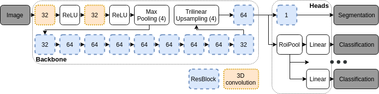
Since we want the resulting tumor representation to be as informative as possible, the head architectures are designed to be very simple, in order to ”motivate” the backbone to generate a comprehensive feature map.
2.1 Backbone
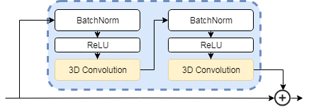
The left side of Fig.1 shows our backbone architecture: it is a relatively simple and fast ResNet-like [14] network adapted for semantic segmentation. The first 2 convolutions are used to prepare the input image for the subsequent residual blocks (ResBlocks, Fig.2). We also apply downsampling and upsampling by a factor of 4 near the network’s input and output respectively in order to decrease the amount of required memory and computation time.
The convolutions and ResBlocks have a kernel of size and padding which effectively leaves the input spatial shape unchanged after such operations, thus for an input image of shape the output feature map will have the shape .
2.2 Network’s heads
Because the segmentation map is a global characteristic of the entire image, for the segmentation task we apply to the entire feature map the head which consists of a single ResBlock. (Fig. 2 shows the structure of a ResBlock.)
The tumor type and localization, however, is a property of a given image area containing a tumor, thus is a local characteristic. That’s why for classification tasks we use a variation of the RoiPool block described in [15], followed by a single linear layer. In our implementation of RoiPool we take a spatial slice corresponding to the tumor’s bounding box and apply global max pooling to it (Fig. 3). As a consequence, the output dimensionality is equal to the number of channels in the feature map generated by the backbone.
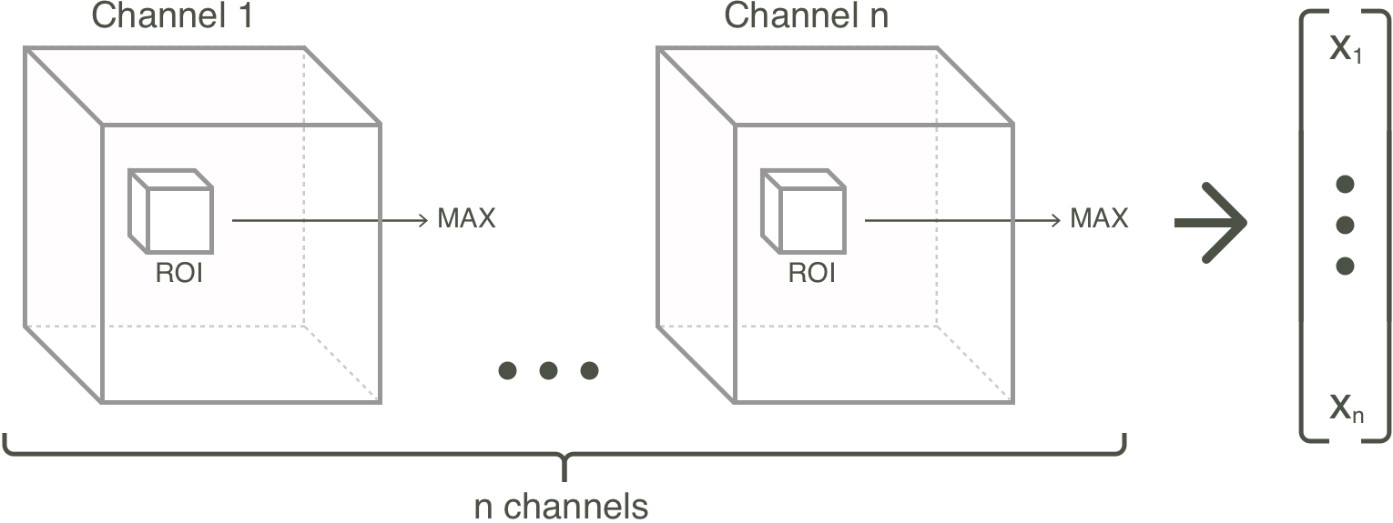
Note that RoiPool is essential for our method because our goal is to obtain fixed-size representations for tumors of different volumes.
2.3 Optimization criterion
For each head, we use cross-entropy as the loss function (binary or multiclass, depending on the task being solved). The final loss being optimized is a weighted sum:
| (1) |
where is either binary or multiclass cross entropy, is the true segmentation mask, is the label for the tumor and task , are the corresponding predictions and - the corresponding weights.
Note that in case of missing metadata for a given tumor and task, the corresponding term can be simply omitted from the final loss.
3 Experiments
3.1 Setup
We train the network for 120 epochs with 200 batches (of size 2) per epoch. Because of technical limitations, instead of feeding entire images into the network, we use patches of size . The patches are picked at random with the sole condition that each selected patch entirely contains a tumor.
In our experiments, we used stochastic gradient descent with Nesterov momentum. In order to avoid the train loss from plateauing we chose a decreasing learning rate policy: the initial learning rate - 0.1 was decreased by a factor of 10 at the 90th and 105th epochs. The weights in the final loss were chosen during the baseline selection stage based on the model’s performance: we ended up using for segmentation and for classification.
For all our experiments we used a random split (80%/20%) of the data with a fixed random seed. The networks were trained on 80% of the data and the other 20% were used for validation.
3.2 Data
| Metastasis | Meningioma | Schwannoma | |
|---|---|---|---|
| # of images | 399 | 339 | 251 |
| # of tumors | 1636 | 414 | 258 |
The data for our experiments was provided by a radiosurgical center that conducts operations on about 400 patients every year. The dataset consists of 989 MRI images in the T1c modality with spatial pixel size and typical image shapes of , see details in Tab. 1. To avoid overfitting, we use only one MRI per patient.
For each image a set of heterogeneous metadata is available: a binary mask of cancerous tissues and a set of labels (in rare cases some of them are missing) including lesion type (metastasis, meningioma, schwannoma), anatomical area such as Region frontalis or Cerebellum (in total we have 11 classes) and various localization: left/right hemisphere, front/rear and upper/lower.
3.3 Validation
Because the notion of tumors similarity is not well-formalized, the validation process is a very complicated task. In order to assess the quality of our approach we make the assumption that similar tumors resemble according to various measurable criteria: e.g. linear size (or volume), type, localization etc. We then evaluate how the distance between the tumors’ embeddings correlates with the resemblance of these criteria.
4 Results
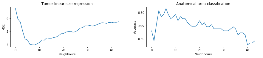
Fig.4 shows the performance of K-Nearest Neighbours models on various tasks depending on the number of neighbours. Note that the performance starts to decrease for , this suggests that the distance between the tumors representations correlates with their similarity. For further experiments we report KNN performances for .
Tab. 2 shows that representations of higher dimensionality expectantly contain more information about some relevant characteristics. We couldn’t go beyond 96 due to technical limitations. As a trade-off between accuracy and training time, in the rest of our experiments we use 64 channels.
![[Uncaptioned image]](/html/1810.09369/assets/x1.png)
![[Uncaptioned image]](/html/1810.09369/assets/x2.png)
Next, we analyze the feasibility of the multitask approach: we trained several networks excluding some tasks from the loss function. The results in Tab.3 show that the multitask approach has a relatively balanced performance compared to the networks trained to solve a single problem, like tumor type classification, or tumors segmentation. This suggests that the network is able to aggregate the additional heterogeneous information contained in tumor labels.
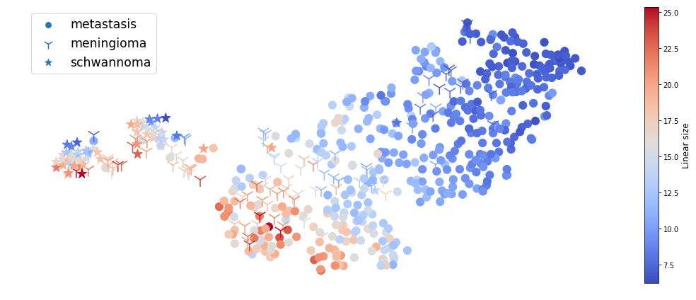
We also visually analyze the representations by decreasing their dimensionality to 2D using using t-SNE. Fig. 5 shows that the representations cluster by type and size. Note the two schwannoma clusters - each cluster corresponds to a brain hemisphere.
In is worth noting that in order to perform the search, our system requires a bounding box of the tumor, in a real world setting the provided bounding box might not be very accurate. In order to we analyze the robustness of our system to such inaccuracies, we added significant distortions to bounding boxes like scaling and translation, so that along each dimension:
| (2) |
We then took the first model from Tab.3 (which saw only accurate boxes during training) and generated representations on the test set based on inaccurate boxes. Tab.4 shows that performance insignificantly declines on some tasks when the boxes are distorted, which means that the system is still able to find relevant tumors even with severely inaccurate bounding boxes.
![[Uncaptioned image]](/html/1810.09369/assets/x3.png)
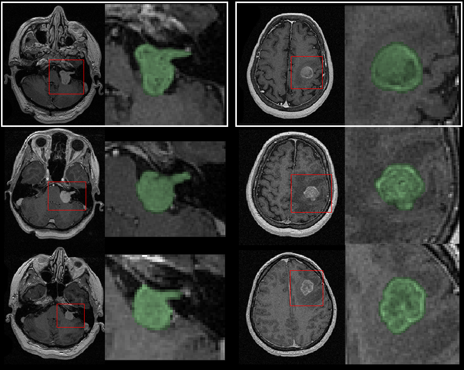
Finally we show some tumor image retrieval examples (Fig.6) for a randomly picked schwannoma and metastasis. Each example shows two tumors proposed by the system: note the similarities such as localization and shape (the resulting tumors are from different patients).
5 Conclusion
We developed a retrieval system that searches for similar brain tumors. The system is based on multitask learning which takes into account heterogeneous metadata available for each dataset entry.
We demonstrated that the distance between tumor representations generated by our method correlates with various measurable tumor characteristics such as type, shape and localization. Also, we showed that the system can be used in the real-world setting by proving that the system performance remains almost unchanged even after significant bounding box distortion.
References
- [1] Jiuxiang Gu, Zhenhua Wang, Jason Kuen, Lianyang Ma, Amir Shahroudy, Bing Shuai, Ting Liu, Xingxing Wang, Gang Wang, Jianfei Cai, et al., “Recent advances in convolutional neural networks,” Pattern Recognition, 2017.
- [2] Geert Litjens, Thijs Kooi, Babak Ehteshami Bejnordi, Arnaud Arindra Adiyoso Setio, Francesco Ciompi, Mohsen Ghafoorian, Jeroen A.w.m. Van Der Laak, Bram Van Ginneken, and Clara I. Sánchez, “A survey on deep learning in medical image analysis,” Medical Image Analysis, vol. 42, pp. 60–88, 2017.
- [3] Sergey Korolev, Amir Safiullin, Mikhail Belyaev, and Yulia Dodonova, “Residual and plain convolutional neural networks for 3d brain mri classification,” in Biomedical Imaging (ISBI 2017), 2017 IEEE 14th International Symposium on. IEEE, 2017, pp. 835–838.
- [4] Konstantinos Kamnitsas, Christian Ledig, Virginia FJ Newcombe, Joanna P Simpson, Andrew D Kane, David K Menon, Daniel Rueckert, and Ben Glocker, “Efficient multi-scale 3d cnn with fully connected crf for accurate brain lesion segmentation,” Medical image analysis, vol. 36, pp. 61–78, 2017.
- [5] Hoo-Chang Shin, Holger R. Roth, Mingchen Gao, Le Lu, Ziyue Xu, Isabella Nogues, Jianhua Yao, Daniel Mollura, and Ronald M. Summers, “Deep convolutional neural networks for computer-aided detection: Cnn architectures, dataset characteristics and transfer learning,” IEEE Transactions on Medical Imaging, vol. 35, no. 5, pp. 1285–1298, 2016.
- [6] Ender Konukoglu, Ben Glocker, Darko Zikic, and Antonio Criminisi, “Neighbourhood approximation using randomized forests,” Medical image analysis, vol. 17, no. 7, pp. 790–804, 2013.
- [7] Amin Katouzian, Hongzhi Wang, Sailesh Conjeti, Hui Tang, Ehsan Dehghan, Alexandros Karargyris, Anup Pillai, Kenneth Clarkson, and Nassir Navab, “Hashing-based atlas ranking and selection for multiple-atlas segmentation,” in International Conference on Medical Image Computing and Computer-Assisted Intervention. Springer, 2018, pp. 543–551.
- [8] Andreia V Faria, Kenichi Oishi, Shoko Yoshida, Argye Hillis, Michael I Miller, and Susumu Mori, “Content-based image retrieval for brain mri: An image-searching engine and population-based analysis to utilize past clinical data for future diagnosis,” NeuroImage: Clinical, vol. 7, pp. 367–376, 2015.
- [9] Katarina Trojachanec, Ivan Kitanovski, Ivica Dimitrovski, and Suzana Loshkovska, “Longitudinal brain mri retrieval for alzheimer’s disease using different temporal information,” IEEE Access, vol. 6, pp. 9703–9712, 2018.
- [10] Ji Wan, Dayong Wang, Steven Chu Hong Hoi, Pengcheng Wu, Jianke Zhu, Yongdong Zhang, and Jintao Li, “Deep learning for content-based image retrieval: A comprehensive study,” in Proceedings of the 22nd ACM international conference on Multimedia. ACM, 2014, pp. 157–166.
- [11] Yu-An Chung and Wei-Hung Weng, “Learning deep representations of medical images using siamese cnns with application to content-based image retrieval,” arXiv preprint arXiv:1711.08490, 2017.
- [12] Adnan Qayyum, Syed Muhammad Anwar, Muhammad Awais, and Muhammad Majid, “Medical image retrieval using deep convolutional neural network,” Neurocomputing, vol. 266, pp. 8–20, 2017.
- [13] Amit Shah, Sailesh Conjeti, Nassir Navab, and Amin Katouzian, “Deeply learnt hashing forests for content based image retrieval in prostate mr images,” Medical Imaging 2016: Image Processing, 2016.
- [14] Kaiming He, Xiangyu Zhang, Shaoqing Ren, and Jian Sun, “Deep residual learning for image recognition,” in Proceedings of the IEEE conference on computer vision and pattern recognition, 2016, pp. 770–778.
- [15] Ross Girshick, “Fast r-cnn,” in Computer Vision (ICCV), 2015 IEEE International Conference on. IEEE, 2015, pp. 1440–1448.