Hyperfine induced transitions ¹S₀ – ³D₁ in Yb

Abstract

Parity violation experiment in Yb is made on the strongly forbidden M1 transition $6s^{2}\,{}^{1}\mathrm{S}_{0}\to 5d6s\,^{3}\mathrm{D}_{1}$. The hyperfine mixing of the $5d6s\,^{3}\mathrm{D}_{1}$ and $5d6s\,^{3}\mathrm{D}_{2}$ levels opens E2 channel, whose amplitude differs for $F$-sublevels of the ${}^{3}\mathrm{D}_{1}$ level. This effect may be important for the experimental search for the nuclear-spin-dependent parity violation effects predominantly caused by the nuclear anapole moment.

.1 Introduction

Up to now the largest parity violation (PV) effect in atomic physics was observed in the transition $6s^{2}\,{}^{1}\mathrm{S}_{0}\to 5d6s\,^{3}\mathrm{D}_{1}$ in ytterbium DeMille (1995); Tsigutkin et al. (2009, 2010); Antypas et al. (2018). The accuracy of the latest experiment Antypas et al. (2018) has reached 0.5%, which allowed to detect isotope dependence of the PV amplitude for even isotopes and obtain the limits on the interactions of additional $Z^{\prime}$ boson with electrons, protons and neutrons. At this level of accuracy it becomes possible to observe a nuclear-spin-dependent (NSD) PV amplitude, which is roughly two orders of magnitude smaller than the nuclear-spin-independent (NSI) PV amplitude. For heavy nuclei this amplitude is dominated by the contribution of the nuclear anapole moment Zel’dovich (1957); Flambaum and Khriplovich (1980); Flambaum et al. (1984). Among several smaller contributions there is one from the weak quadrupole moment Flambaum et al. (2017).

The dominant NSI PV amplitude $6s^{2}\,{}^{1}\mathrm{S}_{0}\to 5d6s\,^{3}\mathrm{D}_{1}$ was calculated in Refs. DeMille (1995); Porsev et al. (1995); Das (1997); Dzuba and Flambaum (2011) and the NSD PV amplitude was calculated in Refs. Singh and Das (1999); Porsev et al. (2000); Dzuba and Flambaum (2011). Experimental detection of the anapole moment in this transition would require precision measurements of the PV amplitudes for different hyperfine components of the $6s^{2}\,{}^{1}\mathrm{S}_{0}\to 5d6s\,^{3}\mathrm{D}_{1}$ transition and comparison with the accurate theory.

The largest contribution to the experimentally observed PV signal comes from the interference term of the PV amplitude and the Stark-induced amplitude Tsigutkin et al. (2010). However, there are other smaller contributions from the interferences with the forbidden M1 transition and the hyperfine induced E2 transition. The former one was measured in Stalnaker et al. (2002) and was found to be:

$$|\langle 5d6s\,^{3}\mathrm{D}_{1}||M1||6s^{2}\,{}^{1}\mathrm{S}_{0}\rangle| =1.33(21)\times 10^{-4}\,\,(\mu_{0})\,,$$ (1)

where $\mu_{0}$ is Bohr magneton. The latter amplitude is not known, but it is expected to be not much smaller. Moreover, it can produce NSD effects by the interference with the main NSI PV amplitude. Here we present calculations of the dominant contribution to this amplitude from the hyperfine mixing between states ${}^{3}\mathrm{D}_{1}$ and ${}^{3}\mathrm{D}_{2}$, which lie only 263 cm^-1apart (see Figure 1).

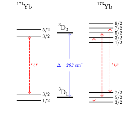
Figure 1: Hyperfine mixings $\varepsilon_{I,F}$ of the $5d6s\,^{3}$D₁ and $5d6s\,^{3}$D₂ levels in odd isotopes ¹⁷¹Yb ($I=\nicefrac{{1}}{{2}}$) and ¹⁷³Yb ($I=\nicefrac{{5}}{{2}}$).

The hyperfine structure of the ${}^{3}\mathrm{D}_{1}$ and ${}^{3}\mathrm{D}_{2}$ levels was measured by Bowers et al. (1999). For example, for the isotope ¹⁷¹Yb the constant $A(^{3}\mathrm{D}_{1})$ was found to be $-2.04$ GHz. The offdiagonal matrix elements of the hyperfine interaction between the levels of the same multiplet are not suppressed, so for the isotope 171 we can expect mixing between these levels on the order of $2\,\mathrm{GHz}/263\,\mathrm{cm}^{-1}\sim 3\times 10^{-4}$. The quadrupole amplitude $6s^{2}\,{}^{1}\mathrm{S}_{0}\to 5d6s\,^{3}\mathrm{D}_{2}$ was measured in Ref. Bowers et al. (1999):

$$|\langle 5d6s\,^{3}\mathrm{D}_{2}||E2||6s^{2}\,{}^{1}\mathrm{S}_{0}\rangle| =1.45(7)\,\,(ea_{0}^{2}),$$ (2)

where $e$ is elementary charge and $a_{0}$ is Bohr radius. The hyperfine mixing of the levels ${}^{3}\mathrm{D}_{1}$ and ${}^{3}\mathrm{D}_{2}$ leads to the hyperfine induced (HFI) quadrupole transitions from the ground state to the state ${}^{3}\mathrm{D}_{1}$. Figure 1 shows that for the isotope 171 there is only one such transition to the sublevel $F=\nicefrac{{3}}{{2}}$; we can estimate its amplitude to be $\sim 4\times 10^{-4}\,(ea_{0}^{2})$. According to this estimate the rate of this HFI transition is about one order of magnitude smaller than the rate of the M1 transition (1). For the isotope 173 there are three such HFI transitions. In this paper we calculate amplitudes of these four HFI transitions.

.2 Hyperfine mixing

Table 1: Nuclear moments of isotopes ¹⁷¹Yb and ¹⁷³Yb.

	171Yb	173Yb	Ref.
Spin	$\nicefrac{{1}}{{2}}$	$\nicefrac{{5}}{{2}}$
$g_{I}$	$0.9838$	$-0.2710$	Kramida et al. (2016)
$Q_{I}$ (bn)		$2.80(4)$	Stone (2005)

The hyperfine mixing coefficients $\varepsilon_{I,F}$ from Fig. 1 between $F$-sublevels of the levels ${}^{3}\mathrm{D}_{1,2}$ for the isotope with spin $I$ are given by the expression:

$$\varepsilon_{I,F} =\frac{1}{-\Delta}\langle^{3}\mathrm{D}_{2},I,F|H_{\mathrm{hf}}|^{3}\mathrm{D}_{1},I,F\rangle\,.$$ (3)

In the following discussion we use atomic units $\hbar=m_{e}=e=1$. In these units $\Delta=E_{{}^{3}\mathrm{D}_{2}}-E_{{}^{3}\mathrm{D}_{1}}=0.001198$. The hyperfine interaction includes magnetic dipole and electric quadrupole parts, which can be written as Kopfermann (1958):

$$H_{\mathrm{hf}} =H_{A}+H_{B}\equiv g_{I}\bm{V}\cdot\bm{I}+Q_{I}T^{(2)}\cdot R^{(2)}\,,$$ (4)

where $g_{I}$ and $Q_{I}$ are $g$-factor and quadrupole moment of the nucleus (see Table 1); $\bm{V}$ and $T^{(2)}$ are irreducible electronic tensors of rank 1 and 2, respectively, and $R^{(2)}$ is the second rank nuclear tensor:

$$R^{(2)}_{i,k} =\frac{3I_{i}I_{k}+3I_{k}I_{i}-2I(2I+1)\delta_{i,k}}{2\sqrt{6}I(2I-1)}\,.$$ (5)

In the following we need the reduced matrix element of this operator:

$$\langle I||R^{(2)}||I\rangle =\sqrt{\frac{(I+1)(2I+1)(2I+3)}{4I(2I-1)}}\,.$$ (6)

Using angular momentum theory Landau and Lifshitz (1977); Sobelman (1979) we can write matrix elements of the operators $H_{A}$ and $H_{B}$ as:

$$\langle J,I,F|H_{A}|J^{\prime},I,F\rangle =(-1)^{I+F+J^{\prime}}\left\{\begin{array}[]{ccc}F&I&J\\ 1&J^{\prime}&I\\ \end{array}\right\}\sqrt{I(I+1)(2I+1)}g_{I}\langle J||V||J^{\prime}\rangle\,,$$ (9)

$$\langle J,I,F|H_{B}|J^{\prime},I,F\rangle =(-1)^{I+F+J^{\prime}}\left\{\begin{array}[]{ccc}F&I&J\\ 2&J^{\prime}&I\\ \end{array}\right\}\sqrt{\frac{(I+1)(2I+1)(2I+3)}{4I(2I-1)}}Q_{I}\langle J||T^{(2)}||J^{\prime}\rangle\,.$$ (12)

In the diagonal case $J=J^{\prime}$ these expressions have the form:

$$\langle J,I,F|H_{A}|J,I,F\rangle =\frac{1}{2}X\cdot\frac{g_{I}\langle J||V||J\rangle}{\sqrt{J(J+1)(2J+1)}}\,,\qquad X=F(F+1)-J(J+1)-I(I+1)\,,$$ (13)

$$\langle J,I,F|H_{B}|J,I,F\rangle =\frac{3X(X+1)-4I(I+1)J(J+1)}{8I(2I-1)J(2J-1)}\cdot\frac{2Q_{I}\sqrt{J(2J-1)}\langle J||T^{(2)}||J\rangle}{\sqrt{(J+1)(2J+1)(2J+3)}}\,.$$ (14)

Comparing Eqs. (13,14) with standard definitions of the hyperfine parameters $A$ and $B$ Radzig and Smirnov (1985), we find:

$$A =\frac{g_{I}\langle J||V||J\rangle}{\sqrt{J(J+1)(2J+1)}}\,,$$ (15)

$$B =\frac{2Q_{I}\sqrt{J(2J-1)}\langle J||T^{(2)}||J\rangle}{\sqrt{(J+1)(2J+1)(2J+3)}}\,.$$ (16)

Experimental and theoretical values of these constants are discussed in Section .5.

Table 2: Relation between hyperfine mixing coefficients $\varepsilon_{I,F}^{A}$ and $\varepsilon_{I,F}^{B}$ and electronic reduced matrix elements.

$I,F$	$\nicefrac{{1}}{{2}},\nicefrac{{3}}{{2}}~{}$	$~{}\nicefrac{{5}}{{2}},\nicefrac{{3}}{{2}}~{}$	$~{}\nicefrac{{5}}{{2}},\nicefrac{{5}}{{2}}~{}$	$~{}\nicefrac{{5}}{{2}},\nicefrac{{7}}{{2}}$
$\frac{\varepsilon_{I,F}^{A}}{\langle^{3}\mathrm{D}_{2}||V||^{3}\mathrm{D}_{1}\rangle}$	$+290.3$	$-164.0$	$-233.7$	$-240.0$
$\frac{\varepsilon_{I,F}^{B}}{\langle^{3}\mathrm{D}_{2}||T^{(2)}||^{3}\mathrm{D}_{1}\rangle}$		$-667.6$	$-362.2$	$+496.0$

According to Eq. (4) the mixing coefficients $\varepsilon_{I,F}$ (3) can be separated in two parts:

$$\varepsilon_{I,F}=\varepsilon_{I,F}^{A}+\varepsilon_{I,F}^{B}\,.$$ (17)

We can now express coefficients $\varepsilon_{I,F}^{A}$ and $\varepsilon_{I,F}^{B}$ in terms of the offdiagonal electronic reduced matrix elements, similar to Eqs. (15,16), where hyperfine constants are expressed in terms of the diagonal reduced matrix elements. To this end we substitute Eqs. (9,12) in (3) and take into account (17). Respective results are summarized in Table 2. Note that the mixings $\varepsilon_{I,F}^{A}$ for both isotopes are comparable, because they are proportional to the nuclear magnetic moment $\mu_{\mathrm{nuc}}=g_{I}I$, rather than $g_{I}$.

.3 HFI transition amplitude $6s^{2}\,{}^{1}\mathrm{S}_{0}\to 5d6s\,^{3}\mathrm{D}_{1}$

The amplitude of the HFI quadrupole transition $6s^{2}\,{}^{1}\mathrm{S}_{0}\to 5d6s\,^{3}\mathrm{D}_{1}$ between hyperfine sublevels is given by:

$$\langle\widetilde{{}^{3}\mathrm{D}_{1}},I,F,M|E2_{q}|^{1}\mathrm{S}_{0},I,F^{\prime}=I,M^{\prime}\rangle=(-1)^{F-M}\\ \times\left(\!\begin{array}[]{ccc}F&1&I\\ -M&q&M^{\prime}\\ \end{array}\right)\langle\widetilde{{}^{3}\mathrm{D}_{1}},I,F||E2||^{1}\mathrm{S}_{0},I,I\rangle\,,$$ (18)

where tilde marks a mixed level. The reduced matrix element is non-zero only because of this mixing with the level ${}^{3}\mathrm{D}_{2}$:

$$\langle\widetilde{{}^{3}\mathrm{D}_{1}},I,F||E2||^{1}\mathrm{S}_{0},I,I\rangle\\ =\varepsilon_{I,F}\,\langle^{3}\mathrm{D}_{2},I,F||E2||^{1}\mathrm{S}_{0},I,I\rangle\,.$$ (19)

The remaining reduced matrix element can be expressed in terms of the respective reduced matrix element for even isotopes (2):

$$\langle^{3}\mathrm{D}_{2},I,F||E2||^{1}\mathrm{S}_{0},I,I\rangle=(-1)^{2I}\\ \times\sqrt{(2I+1)(2F+1)}\left\{\!\begin{array}[]{ccc}0&I&I\\ F&2&2\\ \end{array}\right\}\langle^{3}\mathrm{D}_{2}||E2||^{1}\mathrm{S}_{0}\rangle\\ =(-1)^{F-I}\sqrt{(2F+1)/5}\,\,\langle^{3}\mathrm{D}_{2}||E2||^{1}\mathrm{S}_{0}\rangle\,.$$ (20)

Combining Eqs. (19) and (20) we get the final expression for the HFI amplitude:

$$\langle\widetilde{{}^{3}\mathrm{D}_{1}},I,F||E2||^{1}\mathrm{S}_{0},I,I\rangle\\ =(-1)^{F-I}\varepsilon_{I,F}\,\sqrt{(2F+1)/5}\,\,\langle^{3}\mathrm{D}_{2}||E2||^{1}\mathrm{S}_{0}\rangle\,.$$ (21)

Using the experimental result (2) and the values from Table 2 one can express all HFI amplitudes in terms of the two electronic matrix elements $\langle^{3}\mathrm{D}_{2}||V||^{3}\mathrm{D}_{1}\rangle$ and $\langle^{3}\mathrm{D}_{2}||T^{(2)}||^{3}\mathrm{D}_{1}\rangle$ (see Eq. (4)), which are to be calculated numerically.

.4 NSD PV amplitude $6s^{2}\,{}^{1}\mathrm{S}_{0}\to 5d6s\,^{3}\mathrm{D}_{1}$

Nuclear-spin-dependent PV interaction has the same tensor structure, as the magnetic dipole hyperfine interaction Khriplovich (1991); Ginges and Flambaum (2004):

$$H_{\mathrm{P}} =\frac{G_{F}\kappa}{\sqrt{2}I}\bm{V}_{P}\cdot\bm{I}\,,$$ (22)

where $G_{F}$ is Fermi constant and $\bm{V}_{P}$ is electronic vector operator. The dimensionless constant $\kappa$ is of the order of unity. It includes several contributions, the largest is from the nuclear anapole moment Flambaum and Khriplovich (1980); Flambaum et al. (1984). There are several definitions of this constant in the literature; here we follow Refs. Porsev et al. (2000); Dzuba and Flambaum (2011).

Interaction (22) mixes levels of opposite parity. As a result, the E1 transitions may be observed between the levels of the same nominal parity. In particular, the levels $6s^{2}\,{}^{1}\mathrm{S}_{0}$ and $5d6s\,^{3}\mathrm{D}_{1}$ are mixed with odd-parity levels with $J=1$, which we designate as $n1^{o}$. The two main contributions come from the levels $6s6p\,^{1,3}\mathrm{P}_{1}$ Porsev et al. (2000). The resultant NSD PV E1 amplitude $6s^{2}\,{}^{1}\mathrm{S}_{0}\to 5d6s\,^{3}\mathrm{D}_{1}$ can be written as:

$$E1_{\mathrm{PV}}^{\mathrm{NSD}}\equiv\langle\widetilde{{}^{3}\mathrm{D}_{1}},I,F||E1||\widetilde{{}^{1}\mathrm{S}_{0}},I,I\rangle=(-1)^{2F}\\ \times\sqrt{\frac{(I+1)(2I+1)(2F+1)}{3I}}\left\{\!\begin{array}[]{ccc}F&I&1\\ 1&1&I\\ \end{array}\right\}\,A_{P}\,,$$ (23)

$$A_{P}=\frac{G_{F}\kappa}{\sqrt{2}}\sum_{n}\left[\frac{\langle^{3}\mathrm{D}_{1}||V_{P}||n1^{o}\rangle\langle n1^{o}||E1||^{1}\mathrm{S}_{0}\rangle}{E_{{}^{3}\mathrm{D}_{1}}-E_{n1^{o}}}\right.\\ \left.-\frac{\langle^{3}\mathrm{D}_{1}||E1||n1^{o}\rangle\langle n1^{o}||V_{P}||^{1}\mathrm{S}_{0}\rangle}{E_{{}^{1}\mathrm{S}_{0}}-E_{n1^{o}}}\right]\,.$$ (24)

In Eq. (23) we again mark mixed states with tilde, but this time the mixing is caused by the PV interaction (22).

Expressions (23) and (24) agree with Eq. (8) from Ref. Dzuba and Flambaum (2011) and differ by an overall sign from Ref. Porsev et al. (2000). The difference in sign can be caused by another phase convention, for example, by another order of adding angular momenta Landau and Lifshitz (1977); Sobelman (1979), or by an error. The dependence of the amplitude $E1_{\mathrm{PV}}^{\mathrm{NSD}}$ on the quantum number $F$ is given by Eq. (23), while the amplitude $A_{P}$ has to be calculated numerically. This was already done in Refs. Singh and Das (1999); Porsev et al. (2000); Dzuba and Flambaum (2011).

.5 Numerical results and discussion

Ground state configuration of Yb is [Xe]$4f^{14}6s^{2}$. Most of the low excited states correspond to the excitation of the $6s$ electron. However, there are also states with excitations from the $4f$ subshell. It is important to check whether these states can be neglected in the configuration mixing, reducing the problem to the one with two electrons above closed shells. It was demonstrated in earlier calculations Dzuba and Derevianko (2010); Dzuba et al. (2017, 2018) that such mixing is strong for some low-lying odd-parity states. In particular, the $4f^{13}5d_{5/2}6s^{2}\ (7/2,5/2)^{\rm o}_{1}$ state is strongly mixed with the $4f^{14}6s6p\ ^{1}{\rm P}^{\rm o}_{1}$ state due to small energy interval between them, $\delta E=3789$ cm^-1. Reliable calculations for such states require treating the Yb atom as a 16-electron system. This can be done with the CIPT method developed in Refs. Dzuba et al. (2017, 2018). On the other hand, the mixing of the former state with the $4f^{14}6s6p\ ^{3}{\rm P}^{\rm o}_{1}$ state is small and can be neglected. The energy interval in this case is 10865 cm^-1.

In the present work we are interested in the even-parity states ³D₁ and ³D₂ of the $4f^{14}6s5d$ configuration. The lowest state of the same parity and total angular momenta $J=1$, or $J=2$ containing excitation from the $4f$ subshell is the $4f^{13}5d6s6p\ (7/2,3/2)_{2}$ state at $E$=39880 cm^-1. Corresponding energy interval is large, $\Delta E=15129$ cm^-1, and the mixing in this case can be safely neglected. Therefore, for the purposes of the present work we can treat Yb atom as a system with two valence electrons above closed shells and apply the standard CI+MBPT method (configuration interaction + many-body perturbation theory) Dzuba et al. (1996); Dzuba and Derevianko (2010).

We use the $V^{N-2}$ approximation Dzuba (2005) and perform initial Hartree-Fock (HF) calculations for the Yb III ion with two $6s$ electrons removed. The single-electron basis states are calculated in the field of the frozen core using the B-spline technique Johnson and Sapirstein (1986); Johnson et al. (1988). The effective CI Hamiltonian for two external electrons has a form

$$\hat{H}^{\rm CI}=\hat{h}_{1}(\bm{r}_{1})+\hat{h}_{1}(\bm{r}_{2})+\hat{h}_{2}(\bm{r}_{1},\bm{r}_{2}),$$ (25)

where $\hat{h}_{1}(\bm{r}_{i})$ is a single-electron operator and $\hat{h}_{2}(\bm{r}_{1},\bm{r}_{2})$ is a two-electron operator:

$$\hat{h}_{1}(\bm{r})=c{\bm{\alpha}}{\bm{p}}+(\beta-1)mc^{2}+V^{N-2}(\bm{r})+\hat{\Sigma}_{1}(\bm{r}),$$ (26)

$$\hat{h}_{2}(\bm{r}_{1},\bm{r}_{2})=\frac{e^{2}}{|{\bm{r}_{1}}-{\bm{r}_{2}}|}+\hat{\Sigma}_{2}(\bm{r}_{1},\bm{r}_{2}).$$ (27)

Here $\bm{\alpha}$ and $\beta$ are Dirac matrixes, $V^{N-2}$ is the potential of the Yb III ion including nuclear contribution, $\hat{\Sigma}_{1}$ and $\hat{\Sigma}_{2}$ are correlation operators which include core-valence correlations by means of the MBPT (see Refs. Dzuba et al. (1996); Dzuba and Derevianko (2010) for details).

To calculate transition amplitudes we use the random-phase approximation (RPA). The same $V^{N-2}$ potential as in the HF calculations needs to be used in the RPA calculations. The RPA equations for the Yb III ion can be written as

$$(\hat{H}^{\rm HF}-\epsilon_{c})\delta\psi_{c}=-(\hat{f}+\delta V^{N-2})\psi_{c}.$$ (28)

Here $\hat{H}^{\rm HF}$ is the relativistic HF Hamiltonian (similar to the $\hat{h}_{1}$ operator in (26), but without $\hat{\Sigma}_{1}$), index $c$ numerates states in the core, $\hat{f}$ is the operator of the external field (in our case it is either the nuclear magnetic dipole field, or the nuclear electric quadrupole field), $\delta\psi_{c}$ is the correction to the core single-electron wave function $\psi_{c}$ induced by external field, $\delta V^{N-2}$ is the correction to the self-consistent HF potential due to field-induced corrections to all core wave functions.

Table 3: Hyperfine constants of isotopes ¹⁷¹Yb and ¹⁷³Yb in MHz. Theoretical values are calculated for the nuclear moments from Table 1.

		171Yb	173Yb	Ref.
$A(^{3}\mathrm{D}_{1})$	Exper.	$-2040(2)$	$562.8(5)$	Bowers et al. (1999)
	Theory	$-2349$	$648$	this work
			$596$	Porsev et al. (1999)
$B(^{3}\mathrm{D}_{1})$	Exper.		$337(2)$	Bowers et al. (1999)
	Theory		$249$	this work
			$290$	Porsev et al. (1999)
$A(^{3}\mathrm{D}_{2})$	Exper.	$1315(4)$	$-363.4(10)$	Bowers et al. (1999)
	Theory	$1354$	$-373$	this work
			$-351$	Porsev et al. (1999)
$B(^{3}\mathrm{D}_{2})$	Exper.		$487(5)$	Bowers et al. (1999)
	Theory		$384$	this work
			$440$	Porsev et al. (1999)

The RPA equations are solved self-consistently for all states in atomic core. As a result, the correction to the core potential, $\delta V^{N-2}$ is found. It is then used as a correction to the operator of the external field and the transition amplitudes $T$ are calculated as

$$T_{ab}=\langle a|\hat{f}+\delta V^{N-2}|b\rangle.$$ (29)

Here the states $|a\rangle$ and $|b\rangle$ are two-electron states found by solving the CI+MBPT equations

$$(\hat{H}^{\rm CI}-E_{a})|a\rangle=0\,,$$ (30)

with the CI Hamiltonian given by (25), (26), and (27).

To check the accuracy of this approach we calculate magnetic dipole ($A$) and electric quadrupole ($B$) hyperfine constants for the ³D₁ and ³D₂ states of the isotopes ¹⁷¹Yb and ¹⁷³Yb and compare them with the experiment (see Table 3). One can see that the agreement with the experiment for the constants $A$ is better, than for the constants $B$. For the former the difference between theory and experiment is 3% and 15% respectively, while for the latter it is about 30% for both states. These differences are most likely due to such factors as neglecting higher-order core-valence correlations, incompleteness of the basis, and neglecting hyperfine corrections to the $\hat{\Sigma}$ operators Dzuba et al. (1998). The latter corrections were included in calculation Porsev et al. (1999), where the hyperfine constants (but not the offdiagonal amplitudes) were calculated within the same CI+MBPT method using $V^{N}$ approximation. As we will see below, the dominant mixing is caused by the magnetic hyperfine interaction, where theoretical errors are 15%, or less. We conclude that the accuracy of our calculations is satisfactory for the purposes of the present work.

Numerical values of the offdiagonal hyperfine matrix elements are:

$$\langle^{3}\mathrm{D}_{2}||V||^{3}\mathrm{D}_{1}\rangle =-1.71(26)\times 10^{-6}\,\mathrm{a.u.}\,,$$ (31)

$$\langle^{3}\mathrm{D}_{2}||T^{(2)}||^{3}\mathrm{D}_{1}\rangle =-4.4(13)\times 10^{-8}\,\mathrm{a.u.}\,.$$ (32)

Here we assign 15% error bar to the magnetic dipole term and 30% error bar to the quadrupole term. Comparing these values with the data from Table 2 we see that magnetic term dominates over the electric quadrupole term by roughly an order of magnitude. Using experimental value (2) we get the final values for the HFI amplitudes, which are listed in Table 4. Note that the signs of the amplitudes depend on the phase conventions and we assume positive sign of the amplitude (2).

Table 4: Reduced matrix elements of the transitions $6s^{2}\,{}^{1}\mathrm{S}_{0},I,F^{\prime}=I\to 5d6s\,^{3}\mathrm{D}_{1},I,F$ for the isotopes ¹⁷¹Yb ($I=\nicefrac{{1}}{{2}}$) and ¹⁷³Yb ($I=\nicefrac{{5}}{{2}}$). The HFI quadrupole transition amplitudes (21) are in $ea_{0}^{2}$ and PV E1 transitions (23) are in the units of $A_{P}$, which was calculated in Refs. Singh and Das (1999); Porsev et al. (2000); Dzuba and Flambaum (2011). Subscripts $A$, $B$, and tot. correspond to the contributions from the magnetic dipole and electric quadrupole mixings and the sum of the two.

$I,F$	$\nicefrac{{1}}{{2}},\nicefrac{{1}}{{2}}~{}$	$\nicefrac{{1}}{{2}},\nicefrac{{3}}{{2}}~{}$	$~{}\nicefrac{{5}}{{2}},\nicefrac{{3}}{{2}}~{}$	$~{}\nicefrac{{5}}{{2}},\nicefrac{{5}}{{2}}~{}$	$~{}\nicefrac{{5}}{{2}},\nicefrac{{7}}{{2}}$
$E2_{A}\!\times\!10^{3}$	$0.0$	$+0.643$	$-0.363$	$+0.634$	$-0.752$
$E2_{B}\!\times\!10^{3}$	$0.0$	$0.0$	$-0.039$	$+0.021$	$+0.028$
$E2_{\mathrm{tot.}}\!\times\!10^{3}$	$0.0$	$+0.64(10)$	$-0.40(6)$	$+0.66(10)$	$-0.72(12)$
$E1_{\mathrm{PV}}^{\mathrm{NSD}}/A_{P}$	$+0.667$	$+0.471$	$-0.660$	$+0.231$	$+0.667$

The final errors in Table 4 include experimental error for the amplitude (1) and theoretical errors for amplitudes (31) and (32). Note that the dominant part of these errors is common for all hyperfine transitions and the ratios of the amplitudes are accurate to 3% – 4%. These ratios are particularly important for the interpretation of the PV experiment. Numerical results in Table 4 are in a good agreement with the estimate made above, which was based on the values of the hyperfine constants of the levels ${}^{3}\mathrm{D}_{1}$ and ${}^{3}\mathrm{D}_{2}$.

Table 4 also lists angular factors for the NSD PV amplitude $E1_{\mathrm{PV}}^{\mathrm{NSD}}$ from Eq. (23), which agree with the factors presented in Ref. Dzuba and Flambaum (2011). It is clear that PV amplitude has very different dependence on the quantum numbers $I$ and $F$ than the HFI amplitude (21). This difference is mainly explained by the difference in the respective $6j$-coefficients in Eqs. (9) and (23). The hyperfine interaction mixes level $J=1$ with the level $J=2$, while the PV interaction mixes level $J=1$ with the odd-parity levels $J=1$.

.6 Transition rates

Transition $6s^{2}\,{}^{1}\mathrm{S}_{0,I,I}\to 5d6s\,^{3}\mathrm{D}_{1,I,F}$ may go as $M1$, or as $E2^{\mathrm{HFI}}$. The PV interaction opens two additional channels, $E1^{\mathrm{NSI}}_{\mathrm{PV}}$ and $E1^{\mathrm{NSD}}_{\mathrm{PV}}$. These four transitions have different multipolarity and, therefore, different dependence on the transition frequency and different angular dependence Auzinsh et al. (2010). Because of that we can not directly compare respective amplitudes. Instead we can compare the square roots of the respective transition rates.

The rates for the NSI PV amplitude and $M1$ amplitude do not depend of the quantum numbers $I$ and $F$ and are determined by the expression:

$$W(A1)=\frac{2}{9}(\alpha\omega)^{3}|A1|^{2}\,,$$ (33)

where $A1$ is the respective reduced amplitude. For $M1$ transition this amplitude is given by (1). The NSI-PV amplitude was calculated in Dzuba and Flambaum (2011) to be:

$$\left|E1^{\mathrm{NSI}}_{\mathrm{PV}}\right|=1.85\times 10^{-9}\,.$$ (34)

This value agrees with earlier calculations DeMille (1995); Porsev et al. (1995); Das (1997).

The rates of the NSD-PV and the HFI quadrupole transitions depend on the quantum numbers $I$ and $F$ (see Table 4). The amplitude $E1^{\mathrm{NSD}}_{\mathrm{PV}}$ is roughly two orders of magnitude smaller than (34). The rate of the quadrupole HFI transitions is:

$$W(E2_{I,F})=\frac{(\alpha\omega)^{5}}{25(2F+1)}\left|E2_{I,F}\right|^{2}\,,$$ (35)

where $E2_{I,F}$ is given in Table 4. Putting numbers in Eqs. (33) and (35) we get following ratios for the square roots of the rates:

$$\bigl{(}W(M1)\bigr{)}^{\nicefrac{{1}}{{2}}}:\bigl{(}W(E2_{\nicefrac{{1}}{{2}},\nicefrac{{3}}{{2}}})\bigr{)}^{\nicefrac{{1}}{{2}}}\\ :\bigl{(}W(E1^{\mathrm{NSI}}_{\mathrm{PV}})\bigr{)}^{\nicefrac{{1}}{{2}}}=263:78:1\,.$$ (36)

We see that though $M1$ transition is the largest, the quadrupole HFI transition is not very much weaker. The parity non-conservation rate Khriplovich (1991) ${\cal P}\equiv 2|E1^{\mathrm{NSI}}_{\mathrm{PV}}/M1|\approx 7\times 10^{-3}$.

.7 Conclusions

We calculated hyperfine mixing of the $F$-sublevels of the levels ${}^{3}\mathrm{D}_{1}$ and ${}^{3}\mathrm{D}_{2}$. We found that for both odd-parity isotopes of ytterbium this mixing is dominated by the magnetic dipole term. Using experimentally measured in Ref. Bowers et al. (1999), the $6s^{2}\,{}^{1}\mathrm{S}_{0}\to 5d6s\,^{3}\mathrm{D}_{2}$ transition amplitude we found amplitudes for the hyperfine induced E2 transition amplitudes $6s^{2}\,{}^{1}\mathrm{S}_{0,I,I}\to 5d6s\,^{3}\mathrm{D}_{1,I,F}$. These amplitudes appear to be only one order of magnitude weaker than the respective M1 amplitude (1). Their knowledge is important for the analysis of the on-going measurement of the parity non-conservation in this transition Antypas et al. (2018). These amplitudes can interfere with the Stark amplitude and mimic PV interaction in the presence of imperfections. In particular, they must be taken into account to separate nuclear-spin-dependent parity violating amplitude and to measure anapole moments of the isotopes ¹⁷¹Yb and ¹⁷³Yb. This will not only give us information about new PV nuclear vector moments in addition to the standard magnetic moments, but will also shed light on the PV nuclear forces Flambaum and Khriplovich (1980); Flambaum et al. (1984); Haxton et al. (2001); Ramsey-Musolf and Page (2006); Safronova et al. (2018).