A new spectroscopically-determined potential energy surface and ab initio dipole moment surface for high accuracy HCN intensity calculations

Abstract

Calculations of transition intensities for small molecules like H₂O, CO, CO₂ based on s high-quality potential energy surface (PES) and dipole moment surface (DMS) can nowadays reach sub-percent accuracy. An extension of this treatment to a system with more complicated internal structure – HCN/HNC (hydrogen cyanide/hydrogen isocyanide) is presented. A highly accurate spectroscopically-determined PES is built based on a recent ab initio PES of the HCN/HNC isomerizing system. 588 levels of HCN with $J$ = (0, 2, 5, 9, 10) are reproduced with a standard deviation from the experimental values of $\sigma=0.0373$ cm^-1 and 101 HNC levels with $J$ = (0, 2) are reproduced with $\sigma=0.37$ cm^-1. The dependence of the HCN rovibrational transition intensities on the PES is tested for the wavenumbers below 7200 cm^-1. Intensities are computed using wavefunctions generated from an ab initio and our optimized PES. These intensities differ from each other by more than 1% for about 11% of the transitions tested, showing the need to use an optimized PES to obtain wavefunctions for high-accuracy predictions of transition intensities. An ab initio DMS is computed for HCN geometries lying below 11 200 cm^-1. Intensities for HCN transitions are calculated using a new fitted PES and newly calculated DMS. The resulting intensities compare much better with experiment than previous calculations. In particular, intensities of the H–C stretching and bending fundamental transitions are predicted with the subpercent accuracy.

1 Introduction

The isomerizing system HCN/HNC is important in several areas of science. One significant application of studies HCN/HNC spectra is for astrophysics. Both isomers have been detected in space objects of various types [1, 2, 3], often with abundances far from thermodynamic equilibrium. Observation of both HCN and HNC is facilitated by the fact that both molecules have non-zero dipole moments and thus can be detected by observing pure rotation spectral lines in the submillimeter range or vibrational-rotational lines in the infrared. Along with CO and H₂O, HCN is one of the few molecules that have been detected in the infrared in protoplanetary disks [4]. In the last two years, HCN/HNC has been identified in various astronomical environments including exoplanets [5], satellites [6], comets [7], and planets [8]. Modern observing techniques impose stricter requirements on the accuracy of the available theoretical data [9], namely, transition frequencies and intensities.

In addition to astrophysical studies, the HCN/HNC system is of importance in the quantum chemical analysis. As noted by Mellau [10], the potential energy surface of [H,C,N], in contrast to that of the [H,C,P] system, results in wavefunctions of the two isomers H–CN and CN–H, located in two different minima merging step by step to a single delocalized wavefunction where only a single “combined” H_0.5-CN-H_0.5 molecule exists. Baraban et al.  [11] and Mellau et al.  [12] studied the behavior of this system in the saddle point region. In particular, Mellau et al.  [12] showed that if the saddle point-localized states of the [H,C,N] system can be detected in molecular spectra, they would allow one to define transition states without the need for any quantum frequency analysis.

The various applications of the HCN/HNC spectra require further spectroscopic studies of this molecule. The ability to predict line positions in different frequency ranges and higher temperatures is required for the analysis of the experimental observations of the HCN spectra. In particular it has been suggested that the ratio of HCN to HNC could act as a thermometer in hot atmospheres such as those of cool carbon stars [13].

Last but not least, the rovibrational spectrum of HCN has unique features that, thus far, have provided difficult to describe theoretically. Maki et al.  [14] measured the C$\equiv$N stretching fundamental band and analyzed it in terms of transition dipole moments and Herman-Wallis constants. The unusual intensity patterns for the P- and R-branch of this $(\nu_{1}\nu_{2}^{l}\nu_{3})=(00^{0}1)$ band were explained by large rotation-vibrational interactions meaning that the band dipole was significantly less than permanent dipole moment and, in particular, the transition dipole moment changed sign at a non-zero value of the rotational quantum number, $J$, for almost all isotopologues. The observed band dipole and Herman-Wallis factor values have not so far been accurately reproduced theoretically. In particular, calculations by van Mourik et al.  [15] gave band dipoles which are more than 30 % larger the observed ones. Conversely the dipole values computed by Botschwina et al.  [16] agree well with experiment but their Herman-Wallis factors do not.

Lodi and Tennyson [17] presented a computational strategy to produce accurate line intensities and associated uncertainties. Among other things, the strategy includes computing two sets of nuclear-motion wavefunctions and energy levels using two different, high-quality, PESs. This approach has been employed successfully for a number of studies [18, 19, 20]. A reliable ab initio PES is already available for the HCN/HNC system [21] and the present work provides the second PES needed for such calculations.

As the ab initio PES for the HCN/HNC system computed by van Mourik et al. [15] does not satisfy modern spectroscopic needs, we recently constructed a new one [21]. Despite significantly increasing the accuracy of the predicted rovibrational energy levels, calculations with this PES still do not reach the 0.1 cm^-1 level of accuracy which places most computed line positions within their observed line width in practical spectra. Our experience with the water [22, 23] and ammonia [24] molecules shows that even a small correction to a high-quality ab initio PES can give us a notable improvement in the resulting energy levels. In this context, we note that the previous empirical PES constructed by Varandas and Rodrigues [25] is actually less accurate than our ab initio one [21].

This work is dedicated to the semi-empirical optimization of the PES starting from our recent ab initio PES. The goal of such optimization is twofold. First, the most accurate line positions will be obtained if the optimized PES is used for the rovibrational energy levels calculations. Second, the use of an optimized PES will provide accurate wavefunctions, which can be subsequently used in the high accuracy line intensity calculations. However, to achieve the high accuracy intensity calculations, accurate wavefunctions are not enough. A new, more accurate dipole moment surface (DMS) is also necessary. Such a DMS is also presented here.

The paper is organized as follows. Section 2 gives the technical details of our ab initio calculations and some details of the ab initio energies fit. Section 3 presents the fit of vibrational and rotation-vibrational levels of HCN and HNC; comparisons with the known experimental and ab initio energy levels are also presented. Sector 4 contains the details of dipole moment surface construction. Section 5 provides an intensity analysis for the resulting PES and DMS. In section 6 we discuss our results and directions of the future work.

2 Review of existing surfaces

2.1 Basic ab initio potential energy surface

In a recent paper [21], henceforth referred to as I, we constructed a new ab initio potential energy surface (ab initio PES). Our strategy was similar in spirit with various “model chemistry” schemes used in theoretical thermochemistry [26] and with the focal-point analysis [27]; it was based on a main, high quality PES, to which several correction surfaces were added. We previously used this approach for the water [23], H₂F⁺ [28] and ammonia [24] molecules. But, unlike these ten-electron systems, the electronic structure of [H,C,N] is more complicated because of a multiple (triple) bond, which involves six bonding electrons instead of the usual two ones in a covalent single bond. For water molecule, we achieved 0.1 cm^-1 accuracy ab initio for the rovibrational energies [23]. In the case of HCN/HNC system, calculations with the ab initio PES of I [21] reproduced the extensive set of experimental data below 7000 cm^-1 with a root-mean-square deviation $\sigma=0.37$ cm^-1 when a semi-empirical non-adiabatic correction was applied and $\sigma=1.5$ cm^-1 for levels below 25000 cm^-1 using a purely ab initio approach.

In I we used the functional form suggested by van Mourik et al. [15] as an analytical representation of the whole ab initio PES in Jacobi coordinates:

$$V_{ai}(r,R,\gamma)=\sum_{i,j,k}{A_{ijk}X^{i}(R,r,\gamma)Y^{j}(r,\gamma)P^{k}(\cos{\gamma})},$$ (1)

where $r$ is the CN, $R$ is the “H – center-of-mass of CN” distance and $\gamma$ is the angle between $r$ and $R$, measured in radians, with $\gamma=0$ representing HNC and HCN at $\gamma=\pi$. $X$ and $Y$ are functions of primarily the $R$ and $r$ coordinates, respectively, and are based on a Morse coordinate transformation, with

$$X(R,r,\gamma)=1-e^{-\alpha_{R}(\gamma)[R-R_{e}(\gamma,r)]},$$ (2)

$$Y(r,\gamma)=1-e^{-\alpha_{r}[r-r_{e}(\gamma)]}.$$ (3)

A total of 277 ab initio PES parameters were determined from the fit to 1541 aug-cc-pCV6Z multi-reference configuration interaction (MRCI) ab initio points. More details about the functional form are given by van Mourik et al.  [15] and about the ab initio calculations in I.

2.2 The dipole moment surface

In the work by van Mourik et al.  [15] dipole moments were calculated at the selected 242 grid points (for both HCN and HNC wells) employing cc-pCVQZ CCSD(T) wavefunctions with all electrons correlated. At each grid point dipole moment components were computed via the finite-field method. This DMS was used for calculation of intensities in several linelists [29, 30, 31, 32, 33, 34] including the ExoMol linelist [35], where ab initio and experimental energy levels were merged. These linelists have been used in numerous astronomical studies, the most outstanding of which was the detection of an atmosphere around the super-Earth 55 Cancri e [5]. However, the intensities obtained with this DMS deviate significantly from the experimental ones [14] for the ($0~{}0^{0}~{}1)$ fundamental band. Harris et al.  [29] already noted that the ab initio P branch line intensities are approximately 30 % stronger that the experimental ones and the second minimum of the R branch does not match the experimental minimum.

3 Optimization procedure

3.1 General approach

As we start from an ab initio PES with a high level of accuracy, our primary goal is to tune it to accurately reproduce the experimental data. There are a number of methods of performing such fits, including, for example, morphing [36, 22]. A general method of the optimization developed by Yurchenko et al.  [37] was used. Its main idea is to fit a PES to empirical energies and ab initio grid points simultaneously to avoid nonphysical behavior of the fitting surface in regions, which are poorly constrained by the observed data.

In the present work we construct different semi-empirical PESs for HCN and HNC. In each case we start the fit from the ab initio PES for that well. Performing a unified fit for both wells gave approximately the same result ($\sigma\sim 0.3-0.4$ cm^-1) for both HCN and HNC. This result can be improved by treating each well separately but the unified PES is important for studies of isomerization and states close to the barrier. Conversely, the need for accurate wavefunctions for intensity predictions has been demonstrated in recent studies on other molecules [38, 39], which suggest that for best results $\sigma$ needs to be below 0.05 cm^-1. So far we have only been able to achieve this level of accuracy by using polynomial functions localized in each well.

Considering first HNC, we added an additional surface to the ab initio PES $V_{ai}$ expressed as an analytic polynomial:

$$V^{\rm HNC}(r_{1},r_{2},\theta)=V_{ai}(r_{1},r_{2},\theta)+c_{ijk}{s_{1}}^{i}{s_{2}}^{j}{s_{\theta}}^{k},$$ (4)

$s_{1}=r_{1}-r_{1e}^{\rm HNC},\\ s_{1}=r_{2}-r_{2e}^{\rm HNC},\\ s_{\theta}=\cos{\theta}-\cos{\theta_{e}^{\rm HNC}},\\$ where $r_{1}$ is the CH distance, $r_{2}$ is the CN bond length, $\theta$ is the H-C-N bond angle and the triple $(r_{1e}^{\rm HNC},r_{2e}^{\rm HNC},\theta_{e}^{\rm HNC})$ corresponds to the equilibrium configuration of HNC.

For the HCN well, which is more harmonic, we use a different functional representation. Namely, we fit the same ab initio data from I directly to a polynomial form:

$$V_{\rm ai}^{\rm HCN}(r_{1},r_{2},\theta)=b_{ijk}{s_{1}}^{i}{s_{2}}^{j}{s_{\theta}}^{k}.$$ (5)

$s_{1}=r_{1}-r_{1e}^{\rm HCN},\\ s_{1}=r_{2}-r_{2e}^{\rm HCN},\\ s_{\theta}=\cos{\theta}-\cos{\theta_{e}^{\rm HCN}},\\$ where $r_{1}$ is the CH bond length, and $r_{2}$ and $\theta$ are as defined above, and $(r_{1e}^{\rm HCN},r_{2e}^{\rm HCN},\theta_{e}^{\rm HCN})$ corresponds to the equilibrium configuration of HCN. This fit gives a standard deviation of about 1.5 cm^-1, which can be compared to the global of both wells performed in I, which gave a standard deviation of about 2.6 cm^-1.

$V_{\rm ai}^{\rm HCN}(r_{1},r_{2},\theta)$ provides the starting point for a fit to the observed HCN energy levels, using the same method as in the HNC case:

$$V(r_{1},r_{2},\theta)^{\rm HCN}=V_{\rm ai}^{\rm HCN}(r_{1},r_{2},\theta)+d_{ijk}{s_{1}}^{i}{s_{2}}^{j}{s_{\theta}}^{k}.$$ (6)

Table 1: Coefficients of ab initio points fit $b_{ijk}$ of the HCN polynomial function from eq. (5), powers of 10 in parenthesis.

$i$	$j$	$k$	$b_{ijk}$, cm-1 / Åi+j
0	0	0	-5.82538383470(1)
1	0	0	3.86389321057(2)
0	1	0	-5.73382774051(2)
0	0	1	1.30358201578(4)
2	0	0	1.56450000000(5)
1	1	0	-1.02655390333(4)
1	0	1	-7.34563934810(3)
0	2	0	4.71857396141(5)
0	1	1	-3.35986338937(4)
0	0	2	2.53000000000(3)
3	0	0	-2.99421924819(5)
2	1	0	4.81418477567(3)
2	0	1	-1.48980205956(3)
1	2	0	1.03012191080(3)
1	1	1	1.22487911460(4)
1	0	2	-4.59100323190(3)
0	3	0	-1.05384656549(6)
0	2	1	7.74454197329(3)
0	1	2	1.22794398106(3)
0	0	3	1.60043377884(1)
4	0	0	3.87806313524(5)
3	1	0	-1.89291145139(4)
3	0	1	4.57558177750(3)
2	2	0	-1.59731251862(4)
2	1	1	1.30743572477(4)
2	0	2	6.80295483588(3)
1	3	0	-4.30250739748(3)
1	2	1	-3.34044719190(3)
1	1	2	1.39132320354(4)
1	0	3	-2.22723524934(3)
0	4	0	1.44088983710(6)
0	3	1	-1.14951539583(4)
0	2	2	1.66693158444(4)
0	1	3	1.55423061069(4)
0	0	4	6.75636521337(2)
5	0	0	-3.86359114243(5)
4	1	0	3.94990741828(4)
4	0	1	-8.27443936133(3)
3	2	0	3.95163031431(4)
3	1	1	4.64366715529(4)
3	0	2	-6.21253840400(3)
2	3	0	1.81395172040(4)
2	2	1	-1.63118870226(3)
2	1	2	-3.71978411806(4)
2	0	3	-6.11942762545(3)
1	4	0	-4.77484231577(3)
1	3	1	1.65758045070(4)
1	2	2	-3.30921689766(4)
1	1	3	-1.74115345321(4)
0	5	0	-1.36558717498(6)
0	4	1	6.32814455194(4)
0	3	2	-5.44011053142(3)
0	2	3	-3.08293347406(4)
0	1	4	-2.30801037828(4)
0	0	5	-6.62318144340(2)
6	0	0	2.06164152069(5)
5	1	0	-2.72643462287(4)
5	0	1	1.66406933717(4)
4	2	0	-9.06418473036(4)
4	1	1	-9.89426326122(4)
4	0	2	-6.23124778630(3)
3	3	0	2.20380959568(4)
3	2	1	-9.35548681411(4)
3	1	2	-1.61886146354(4)
3	0	3	1.16982465743(4)
2	4	0	0.00000000000(0)
2	3	1	0.00000000000(0)
2	2	2	-1.27099007662(4)
2	1	3	2.31053677106(4)
2	0	4	5.16397238424(3)
1	5	0	0.00000000000(0)
1	4	1	0.00000000000(0)
1	3	2	0.00000000000(0)
1	2	3	6.17471253018(4)
1	1	4	1.20224840548(3)
1	0	5	-1.57260975308(3)
0	6	0	3.62568390524(5)
0	1	5	1.40150909942(4)
0	2	4	1.68845345324(4)
0	3	3	1.55751022655(4)
0	2	4	0.00000000000(0)
0	1	5	0.00000000000(0)
0	0	6	-4.05714839862(2)

Table 2: Optimized coefficients $d_{ijk}$ of the HCN polynomial function from eq. (6), powers of 10 in parenthesis.

$i$	$j$	$k$	$d_{ijk}$, cm-1 / Åi+j
1	0	0	-5.7427163997318(1)
0	1	0	1.3345870332940(2)
0	0	1	2.4975542880134(1)
2	0	0	5.1497044820851(1)
1	1	0	-1.4358942155508(2)
1	0	1	-6.4634883126558(1)
0	2	0	-1.6859489693547(2)
0	1	1	-1.2665929510125(0)
0	0	2	-4.9044301624532(1)
3	0	0	2.2987168749403(2)
0	3	0	-1.1715811331028(3)
0	0	3	3.4727493153491(1)

Table 3: Optimized coefficients $c_{ijk}$ of the HNC polynomial function from eq. (4), powers of 10 in parenthesis.

$i$	$j$	$k$	$c_{ijk}$, cm-1 / Åi+j
0	0	0	$-2.5228259785515(3)$
1	0	0	$3.1876702203250(2)$
0	1	0	$-6.6678874296762(3)$
0	0	1	$-2.4842036191744(3)$
2	0	0	$-1.5885178372949(3)$
1	1	0	$2.0186290559122(3)$
1	0	1	$6.6308401256739(3)$
0	2	0	$2.1284923915787(4)$
0	1	1	$-3.3052835812817(3)$
0	0	2	$-1.7868381384170(4)$
3	0	0	$2.1113127247948(3)$
0	3	0	$-2.3906844780148(4)$
0	0	3	$-1.8174121247121(5)$
4	0	0	$3.1069836700747(3)$
0	0	4	$-1.0227632425463(6)$
0	0	5	$-1.6015153206752(6)$

3.2 Nuclear motion calculations

The vibrational energy levels were calculated using the DVR3D program suite [40]. The parameters used are presented in Table LABEL:tab:dvr_param; Morse-like oscillators were used for the radial basis functions. We include almost all corrections used in the ab initio PES: adiabatic and relativistic correction surfaces and a nonadiabatic correction (by choosing atomic masses), to get the best starting point for fitting. More details about corrections are given in I.

Table 4: Input parameters for DVR3DRJZ module of DVR3D [40]; the Morse parameters are in atomic units, atomic masses are in Da.

Parameter	Value	Description
NPNT1	40	No. of $r_{1}$ radial DVR points (Gauss-Laguerre)
NPNT2	40	No. of $r_{2}$ radial DVR points (Gauss-Laguerre)
NALF	50	No. of angular DVR points (Gauss-Laguerre)
NEVAL	950	No. of eigenvalues/eigenvectors required
MAX3D	5500	Dimension of final vibrational Hamiltonian
XMASS (H)	1.007825	Mass of hydrogen atom
XMASS (C)	12.000000	Mass of carbon atom
XMASS (N)	14.003074	Mass of nitrogen atom
$r_{1e}$	2.3	Morse parameter ($r_{1}$ radial basis function)
$D_{1e}$	0.1	Morse parameter ($r_{1}$ radial basis function)
$\omega_{1e}$	0.0105	Morse parameter ($r_{1}$ radial basis function)
$r_{2e}$	3.2	Morse parameter ($r_{2}$ radial basis function)
$D_{2e}$	0.1	Morse parameter ($r_{2}$ radial basis function)
$\omega_{2e}$	0.004	Morse parameter ($r_{2}$ radial basis function)

3.3 The HCN fit

We took $(r_{1e},r_{2e},\theta_{e})$ = (1.066 Å, 1.153 Å, $180.0^{\circ})$ as the minimum in the HCN well from the ab initio PES. Mellau [41] reported experimental characterization of all 3822 eigenenergies of HCN up to 6880 cm^-1 relative to the ground state using high temperature hot gas emission spectroscopy. In nearly all cases these empirical energy levels are accurate to better than 0.0004 cm^-1. This dataset was used in this work. The set of ab initio and optimized polynomial coefficients from eq. (6) are presented in Tables LABEL:tab:hcn_constai and 2, respectively.

HCN vibrational ($J=0$) energy levels are presented in table LABEL:tab:hcn_levels. A table of the calculated levels with $J=2$ is given in the supplementary material. The standard deviation for the levels with $J=(0,2,5,9,10)$ is $\sigma=0.0373$ cm^-1.

Table 5: HCN energy levels computed using our recent ab initio PES [21] and the new PES, experimental data are taken from Mellau et al.  [41]. All values are in cm^-1. Experimental uncertainties for the levels are about 10^-4 cm^-1.

($\nu_{1}$	$\nu_{2}$	$\nu_{3}$)	Obs.	$\text{Obs.}-\text{calc.}$	$\text{Obs.}-\text{calc.}$
				(ab initio [21])	(this work)
0	2	0	1411.4135	0.18	-0.0357
0	0	1	2096.8455	0.67	-0.0428
0	4	0	2802.9587	0.71	-0.0306
1	0	0	3311.4771	-1.25	-0.0052
0	2	1	3502.1211	0.14	-0.0011
0	0	2	4173.0709	1.09	-0.0712
0	6	0	4174.6086	-0.08	0.0132
1	2	0	4684.3100	-1.93	-0.0291
0	4	1	4888.0393	1.13	-0.0337
1	0	1	5393.6977	-0.68	-0.0132
0	8	0	5525.8128	-1.54	0.0138
0	2	2	5571.7343	0.23	0.0216
1	4	0	6036.9601	-0.97	-0.0195
0	0	3	6228.5983	1.34	-0.0640
0	6	1	6254.4059	0.63	-0.0567
2	0	0	6519.6105	-2.58	-0.0116
1	2	1	6760.7051	-1.24	-0.0374
0	10	0	6855.4431	-2.89	-0.0585
0	4	2	6951.6830	1.58	-0.0531
1	6	0	7369.4438	-	0.0418
1	0	2	7455.4235	0.49	-0.0219
0	8	1	7600.5358	-	-0.0478

3.4 The HNC fit

We took $(r_{1e},r_{2e},\theta_{e})$ = (2.187 Å, 1.187 Å, $0.0^{\circ})$ as the minimum of the HNC well. The set of optimized polynomial coefficients from eq. (4) are presented in table 3.

As for HCN, Mellau [10, 42, 43] performed extensive measurements of HNC energy levels and these data were used for the fit. HNC vibrational ($J=0$) energy levels are given in table LABEL:tab:hnc_levels, the standard deviation for the levels with $J=(0,2)$ is $\sigma=0.37$ cm^-1. A table of the calculated levels with $J=2$ is given in the supplementary material.

Table 6: HNC vibrational energy levels computed with our recent ab initio PES [21] and the new PES, experimental data are taken from Mellau [10, 42, 43]. All values are in cm^-1.

($\nu_{1}$	$\nu_{2}$	$\nu_{3}$)	Obs.	$\text{Obs.}-\text{calc.}$	$\text{Obs.}-\text{calc.}$
				(ab initio [21])	(this work)
0	2	0	926.5032	0.82	-0.4210
0	4	0	1867.0587	4.61	-0.1969
0	0	1	2023.8594	0.43	0.0390
0	6	0	2809.2876	9.45	0.2325
0	2	1	2934.8188	1.11	-0.4151
1	0	0	3652.6566	-3.78	0.4372
0	8	0	3743.7641	11.06	-0.2029
0	4	1	3861.4285	4.29	0.1328
0	0	2	4026.3981	1.96	-0.0580
1	2	0	4534.4499	-2.89	-0.2187
0	6	1	4790.8597	9.58	-0.6460
0	2	2	4921.2449	2.20	-0.7661
1	4	0	5428.9856	1.83	-0.3650
1	0	1	5664.8527	-2.36	-0.5914
0	4	2	5833.4283	7.31	-0.0032
1	6	0	6322.7195	8.00	0.2206
1	2	1	6532.4023	-1.12	-0.0580
2	0	0	7171.4016	-0.58	0.0447
1	8	0	7205.1561	9.06	-0.0174
1	4	1	7413.9507	-	-0.0536

4 Dipole moment surface construction

4.1 Electronic structure computations

As described elsewhere [44], the external field calculation (ED) of the dipole moment points is preferable to the expectation value method (XP). The ab initio surface computed for HCN in I gives, as a byproduct, the expectation values of dipole moments. The corresponding PES points are of high accuracy, so we thought that we could construct a good DMS using these byproduct dipole moments. We fitted them to a functional form similar to the one used below and the results were very poor; some computed intensities differed by 50 % from the observed values and thus were much worse than the values given by the ED DMS obtained 15 year ago using an aug-cc-pvQZ basis set and the default MOLPRO complete active space (CAS) [15]. This demonstrates once more the importance of using the ED method to compute dipole moments.

We employed the IC-MRCI all-electrons method for dipole moment calculations as programmed in MOLPRO [45]. In I, we gave a detailed description of the choice of the CAS. Selection of the CAS is very important as it strongly influences accuracy of the calculations. Here, for the dipole moment calculations, we selected the same CAS as used in I for creating the ab initio PES. Using the aug-cc-pCV6Z basis used in I proved to be prohibitively expensive for the dipole moments calculations, as every dipole point requires 4 independent calculations of the energies in an external field. We therefore used an aug-cc-pCV5Z basis instead to reduce computer time. We calculated 902 DMS points. In I the best result was achieved using the Pople relaxed correction, so here we decided to use the same MRCI correction for construction of the DMS. Also a relativistic correction, mass-velocity plus first-order Darwin term (MVD1) as produced by MOLPRO was added. Beyond Born-Oppenheimer effects have been shown to be fairly small [46] and are not considered here.

4.2 Fitting the DMS

A polynomial form similar to eq. (5) was used to represent the DMS:

$$\mu_{x}(r_{1},r_{2},\theta)=t_{ijk}{s_{1}}^{i}{s_{2}}^{j}{s_{\theta}}^{k},$$ (7)

$$\mu_{z}(r_{1},r_{2},\theta)=u_{ijk}{s_{1}}^{i}{s_{2}}^{j}{s_{\theta}}^{k}.$$ (8)

A total of 82 parameters (for each component) were determined from the fit to 902 dipole moment points that resulted in a standard deviation of $2.56\times 10^{-6}$ a.u. from the fitted surface for the $x$ dipole component, and $5.16\times 10^{-6}$ a.u. for the $z$ component.

5 Intensity analysis

We computed transition intensities for HCN transitions up to $J=10$ for wavenumbers up to 7 200 cm^-1 using the PESs and DMSs described above. The transition intensities of each of the fundamentals has recently been measured experimentally and they are detailed below.

5.1 PES part

Table II in the Supplementary Material shows the differences in intensities caused by the improvement in accuracy of wavefunctions for lines with intensities higher than $10^{-23}$ cm/molecule. These transitions were grouped by differences in percentages and the results of this are presented in the table 7. It is apparent that transition intensities obtained with the same DMS may vary significantly with wavefunctions calculated using the ab initio PES from I or the new fitted one.

Table 7: Comparison of HCN intensities computed using potential surfaces by van Mourik et al.  [15], Makhnev et al. [21] (I) and using the new fitted PES. The comparison is made for 550 transitions between the states with $J\leq 5$. The DMS used in the calculations was taken from [15]. The percentage differences are computed as $(I_{1}/I_{2}-1)\cdot 100$ %.

	$N_{\textrm{lines}}$ between PESs from:
Intensity difference	[15] – [21]	[21] – this work
	(old – new ab initio)	(new ab initio – fitted)
$<1~{}\%$	255	487
$1-5~{}\%$	232	35
$5-10~{}\%$	22	18
$>10~{}\%$	41	10

5.2 DMS part

We compared our predicted intensities with available experimental data to verify the quality of our surfaces. The mean differences between the experimental and calculated intensities are shown in table 8. For all fundamental transitions (bold) the new DMS better reproduces the measurements. Accuracy approaching 1 %  is achieved for two of the fundamentals, the H – CN stretch and the bend. These predictions lie within the quoted experimental uncertainties. The behavior of the CN-stretch is described in detail below.

The region about the HCN well has previously been extensively studied theoretically; the improved accuracy of our calculated intensities for the fundamental bands lies, mostly, in two factors: use of an increased density of dipole moment points and a larger basis set. The influence of both of these factors for each group of transitions is considered separately.

We also computed and fitted about 300 dipole points near the HCN minimum with the same level of theory as that used by van Mourik et al.  [15] and fitted these using eqs. (7) and (8). Intensities obtained using these points help to quantify the dependence of the results on the number of ab initio points used in the fit, since only 115 points were used to determine the DMS by van Mourik et al.  [15]. Below we call this new DMS the “new local” one, the DMS from van Mourik et al. [15] is described as the “old global” one, and our improved DMS (described in section 4) is simply called the ’‘new” one.

Table 8: Standard deviation of difference ($\varepsilon=I_{\text{calc}}/I_{\text{exp}}-1,\,\%$) between the calculated and observed HCN transition intensities.

Transition	DMS [15]	DMS (this work)	$N_{\text{lines}}$	Exp. uncert., %	Exp. source
$\nu_{1}$	1.60	1.24	40	2-3	[47]
$\nu_{1}+\nu_{2}^{1}-\nu_{2}^{1}$, (e/f)	5.21/5.05	5.23/5.07	35/41	4-5	[47]
$\nu_{2}^{1}$	2.40	1.48	50	2-3	[48]
$2\nu_{2}^{0}$	2.31	0.98	40	2-3	[49]
$2\nu_{2}^{0}-\nu_{1}^{1}$	5.89	5.80	36	4-6	[48]
$2\nu_{2}^{2}-\nu_{1}^{1}$	6.95	6.59	45	4-10	[48]
$3\nu_{2}^{1}-\nu_{2}^{1}$ , (e/f)	3.99/4.87	3.98/4.68	33/35	4-6	[49]
$2\nu_{2}^{2}$	6.30	6.74	37	[5]a	[50]
$3\nu_{2}^{3}$	12.32	15.39	14	[5]a	[50]
$2\nu_{2}^{2}+\nu_{3}$	19.54	14.10	30	[5]a	[50]
$\nu_{1}+2\nu_{2}^{2}$	48.99	23.95	19	[5]a	[50]
$(\nu_{3})^{b}$	34.42	16.58	19	5	[14]
a Maki et al.  [50] do not give experimental uncertainties. The value $5\%$ is based on
previous work of Maki group [14] with the same experimental setup.
b P-branch only.

5.2.1 HCN $\nu_{1}$, $\nu_{1}+\nu_{2}^{1}-\nu_{2}^{1}$ transitions (stretching of H–C)

Experimental data were taken from Devi et al.  [47]

The H–C coordinate comprises the strongest type of covalent chemical bond – a $\sigma$ bond. But since this bond is single, its properties can be described relatively easily, and a satisfactory level of accuracy for the H–C vibrational mode had been already achieved some time ago. Figure 1 shows an improvement between the calculation performed with the “old global” DMS [15] (red) and the one with the new DMS (blue) for a $\nu_{1}$ transition. The standard deviation of the intensities for this band improves from 1.60 to 1.24 %. For the hot band $\nu_{1}+\nu_{2}^{1}-\nu_{2}^{1}$ (figure 1) there are no significant changes but there is a huge difference between the corresponding $e/f$ transitions.

For $\nu_{1}$ transitions the difference between the “old global” and the recalculated “new local” DMSs is much smaller than 1 %, so there is only a weak dependence on the number of points here, and the main reason for the improved accuracy of calculations achieved with the new DMS is a better basis set used in the ab initio calculations.

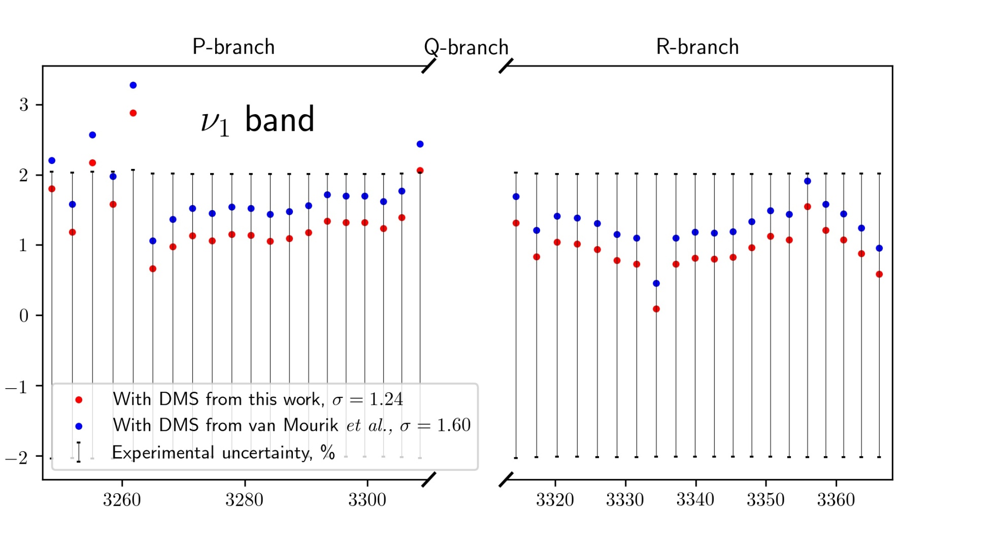
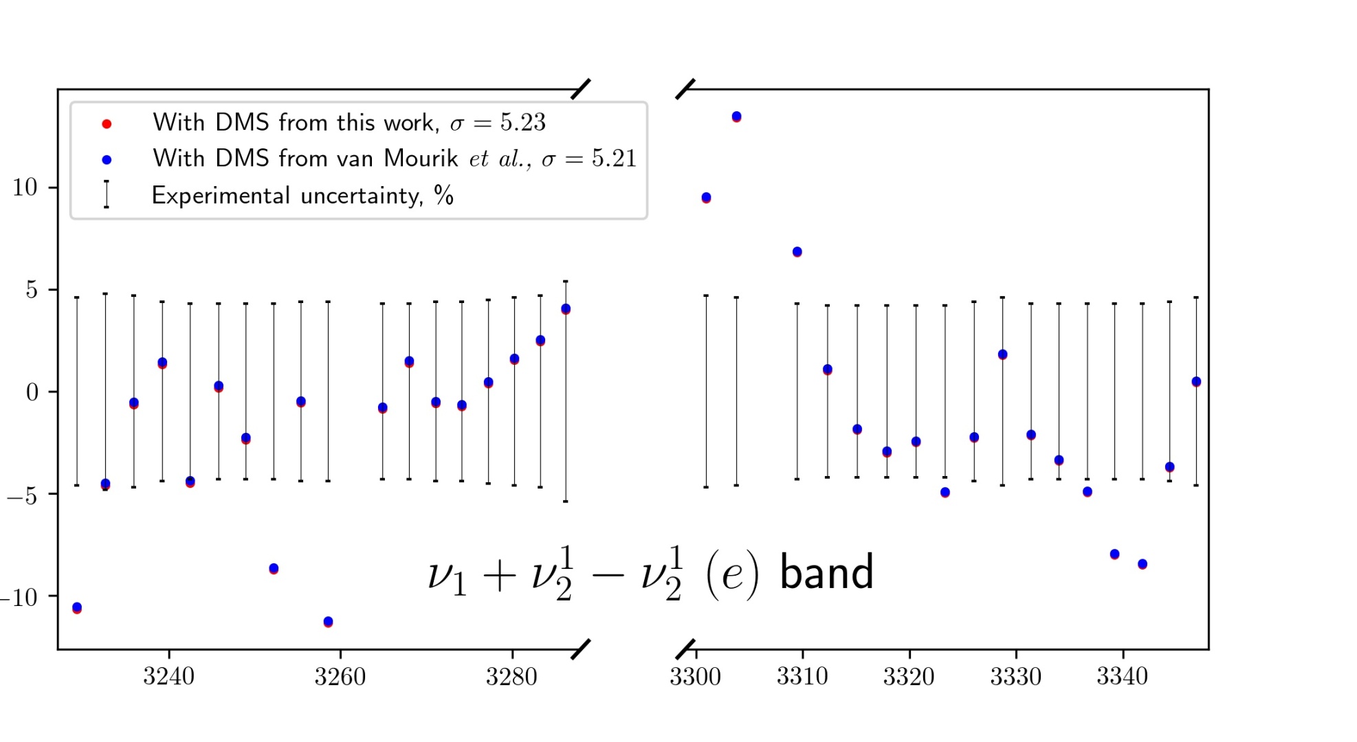
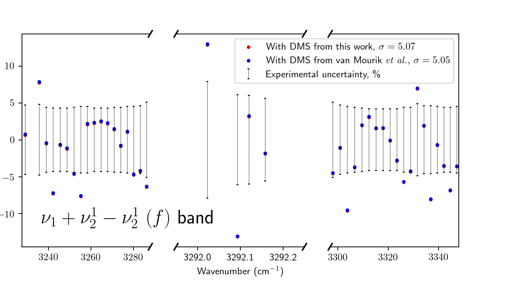
Figure 1: Comparison of HCN line intensities for the $1000-0000$ (top), $1110-0110$(e) (middle) and $1110-0110$(f) (bottom) bands.

5.2.2 HCN $\nu_{2}^{1}$, $2\nu_{2}^{0}$, $2\nu_{2}^{0}-\nu_{2}^{1}$, $2\nu_{2}^{2}-\nu_{1}^{1}$, $3\nu_{2}^{1}-\nu_{2}^{1}$ transitions (bending)

Experimental data were taken from Devi et al.  [49] and Smith et al.  [48]

In contrast to the H–C stretch, bending motions probe a weaker $\pi$-bond and harder to analyze with the same level of accuracy. But for the $\nu_{2}^{1}$ and $2\nu_{2}^{0}$ transitions (see figure 2) the intensity differences are reduced from 2.40 and 2.31 % to 1.48 and 0.98 %, respectively. The accuracy of “hot” transitions ($2\nu_{2}^{0}-\nu_{2}^{1}$ – figure 3, $2\nu_{2}^{2}-\nu_{1}^{1}$ – figure 3, $3\nu_{2}^{1}-\nu_{2}^{1}$ – figures 4) intensity calculations is almost unimproved.

For this group of transitions the dependence of the computed intensities on the number of dipole points used increases to 8-12 %. The resulting percent and sub-percent accuracy we obtain relies on a combination of both factors: increased number of points and improved level of theory.

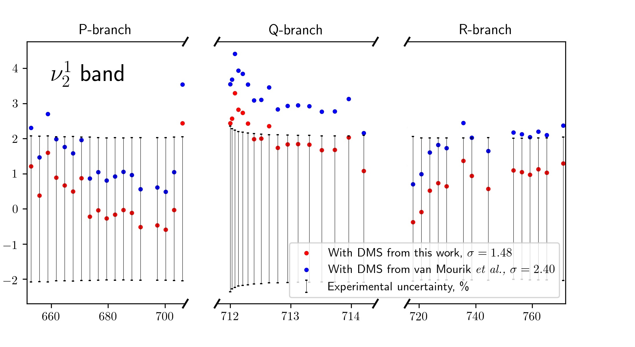
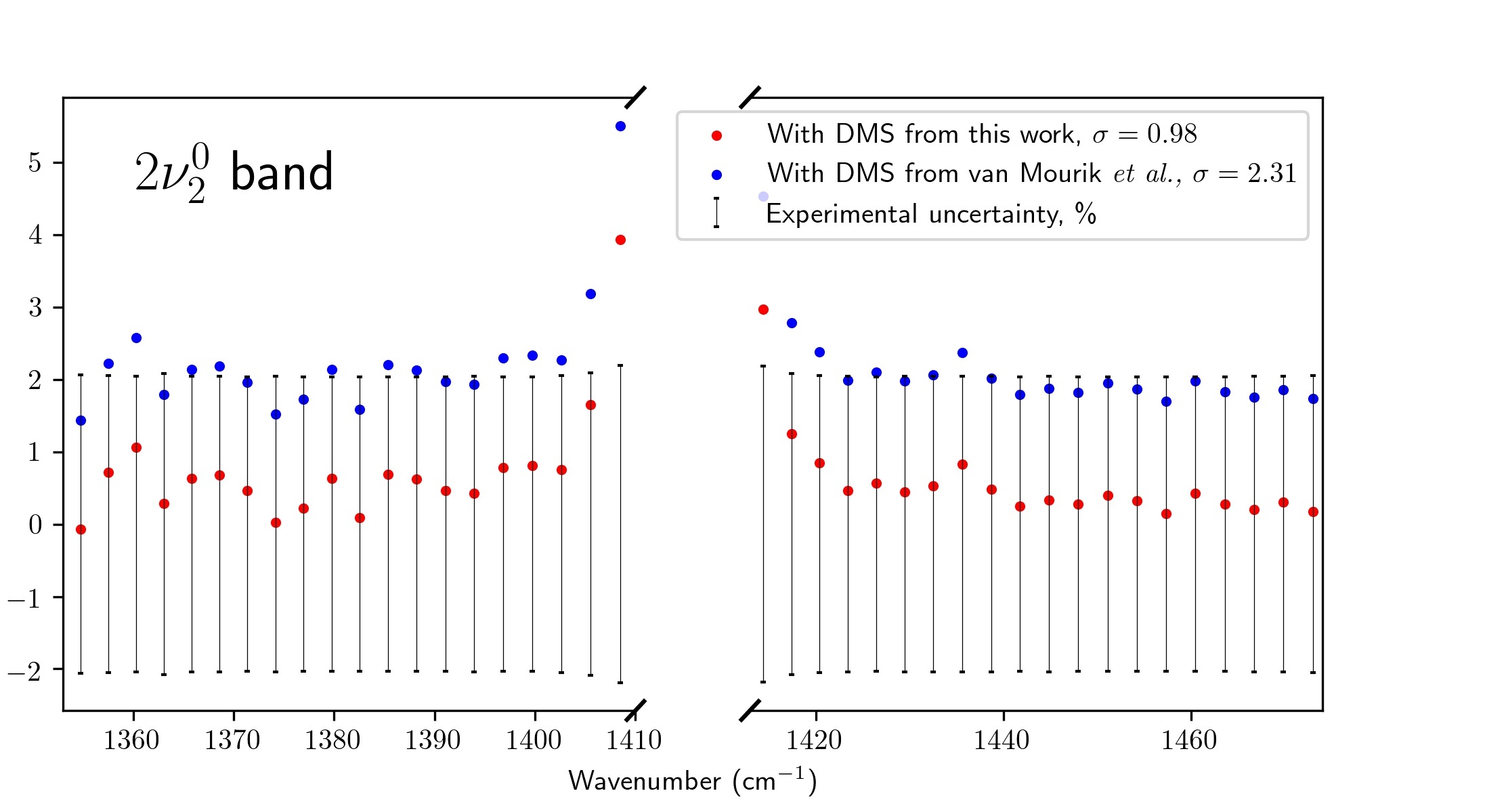
Figure 2: Comparison of HCN line intensities for the $0110-0000$ (upper) and $0200-0000$ (lower) bands.

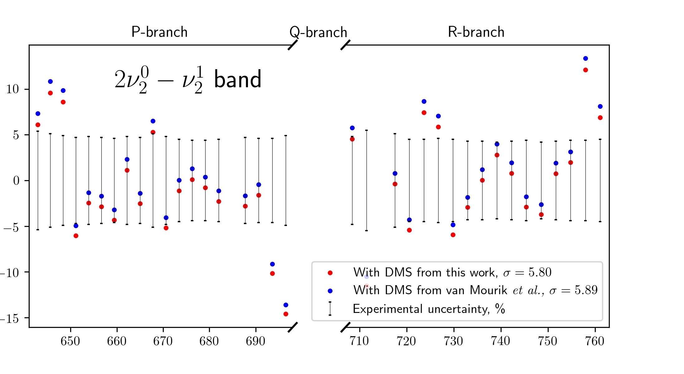
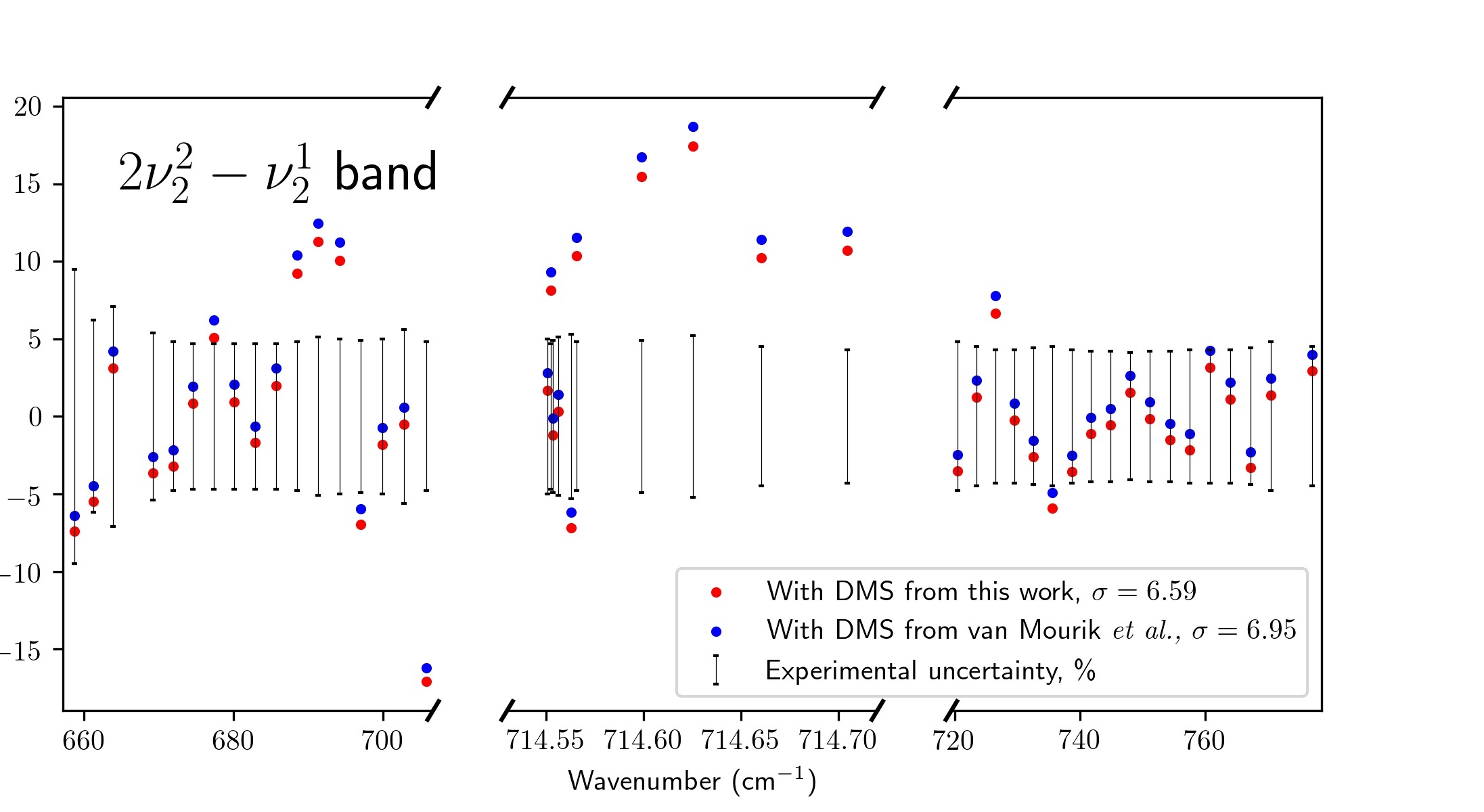
Figure 3: (Comparison of HCN line intensities for the $0200-0110$ (upper) and $0220-0110$ (lower) bands.

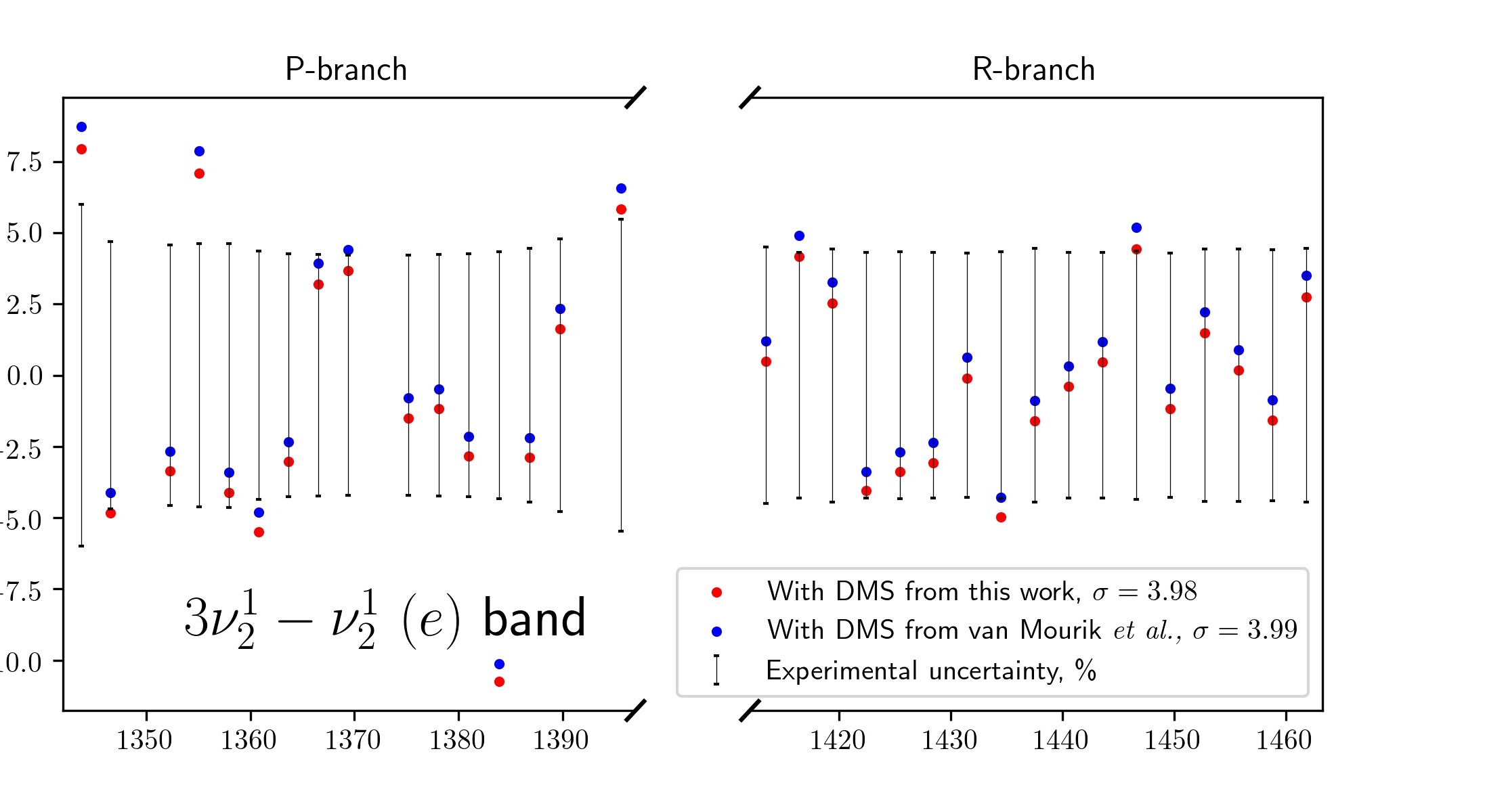
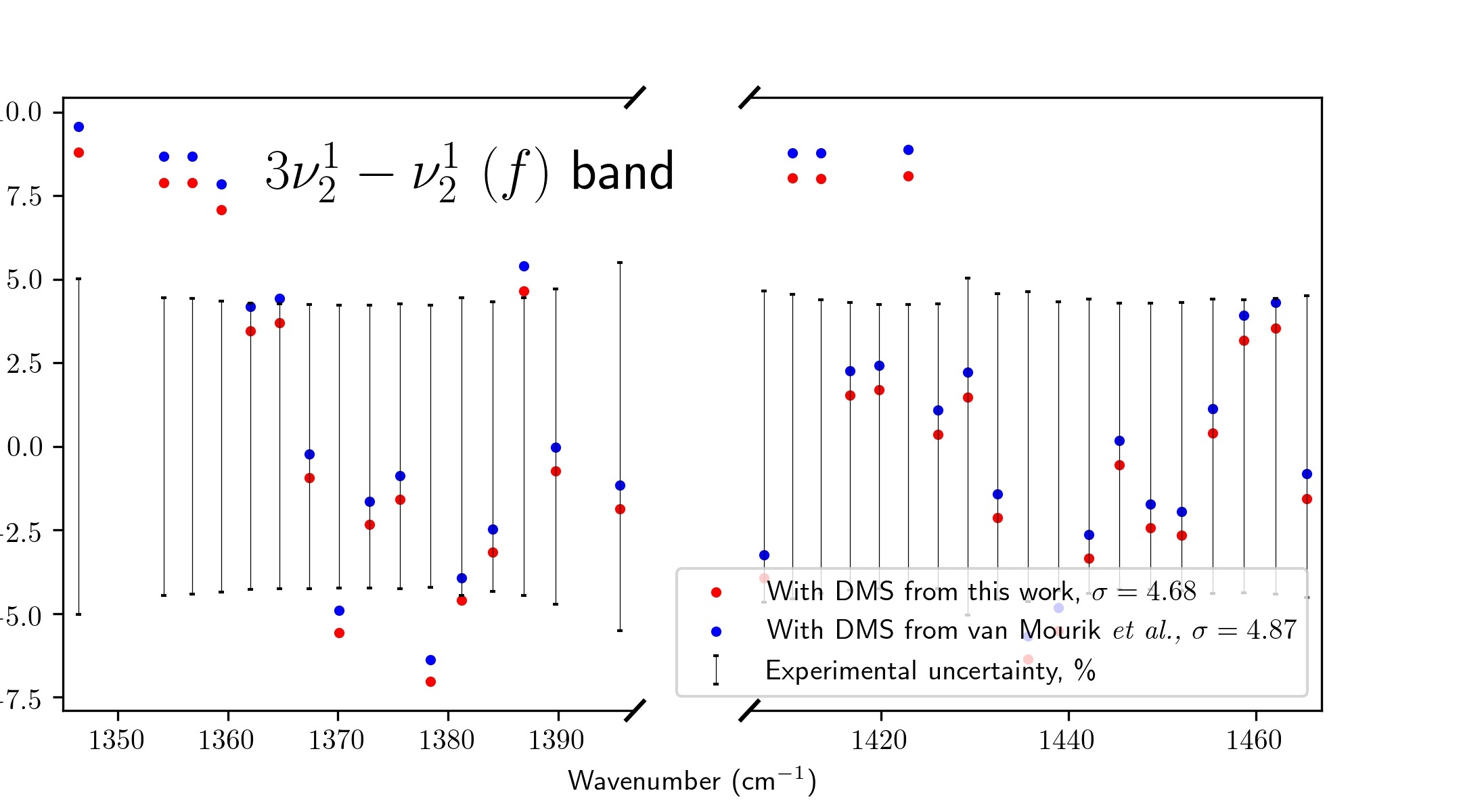
Figure 4: Comparison of HCN line intensities for the $0310-0110$(e) (upper) and $0310-0110$(f) (lower) bands.

5.2.3 HCN $\nu_{3}$ transitions (stretching C$\equiv$N)

The atoms in the CN-stretch are connected by a triple bond ($\sigma+2\pi$) involving six electrons, which is much harder to handle theoretically. A comparative study of this CN-mode was performed by Maki et al.  [14], who connected the existence of a second minimum in the intensity of the R branch transitions near R(7) for the main isotopologue with strong vibration-rotation interaction for this mode. The minimum (or the gap) shifts between isotopologues and can also be detected in the (01¹1–01¹0) hot band. Intensities computed for this stretch mode with the “old global” DMS by Harris et al.  [29] are of the same order of magnitude.

Figure 6 shows the calculated intensities of the P-branch from the (0001–0000) band with the “old global” (blue), the “new local” (black) and the new (red) DMSs. The experimental data are taken from Maki et al.  [14] (green). Here increasing the number of calculated points changes the calculated intensities by about 20 %.

Intensities calculated with the new DMS give improved agreement: the deviation from the experimental data are 21.5 % in comparison with 36.2 % for the “old global” DMS (see figure 5). It is likely that further improvement will require both higher level calculations and a denser grid.

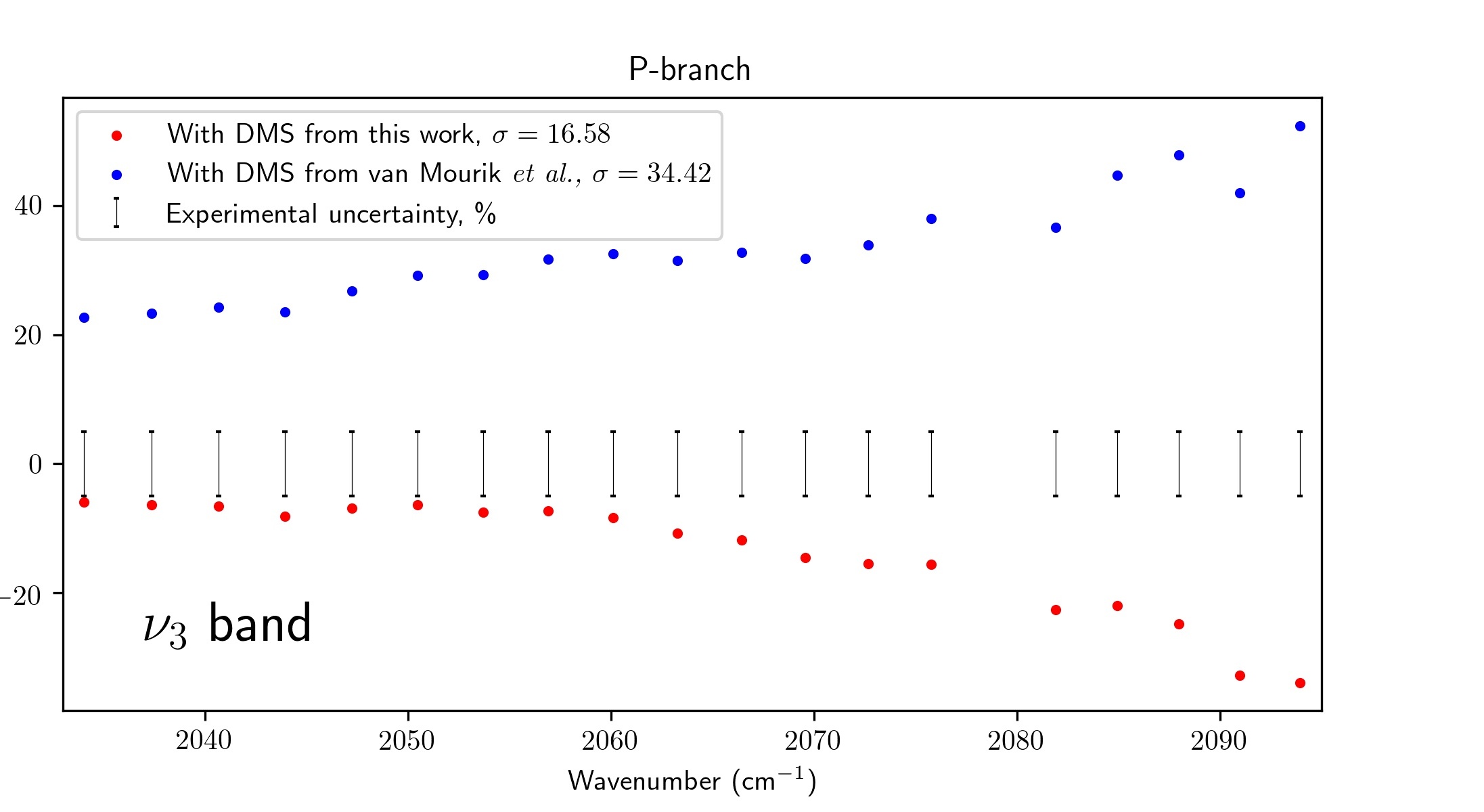
Figure 5: Comparison of line intensities for the ($0001-0000$) transition, P-branch.

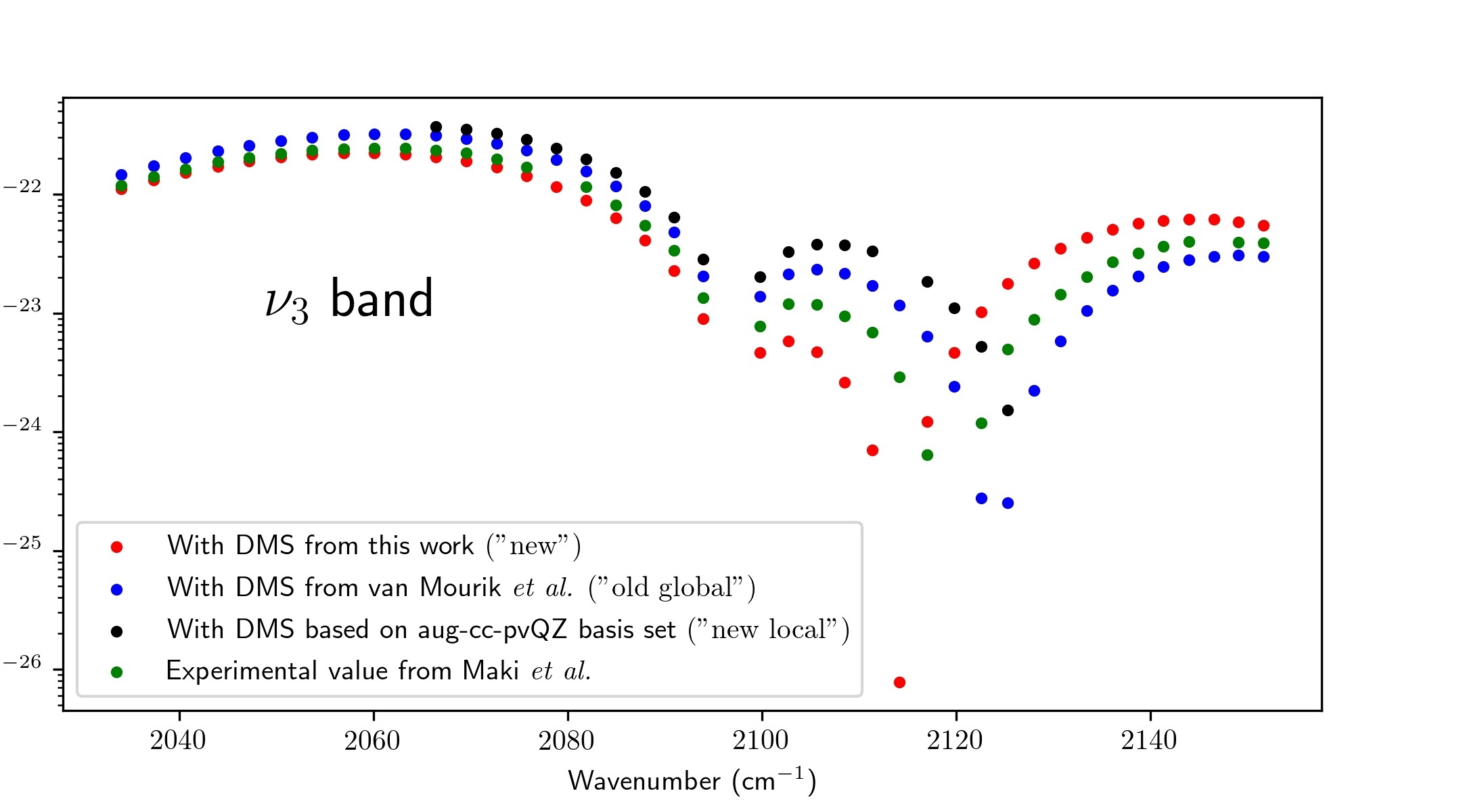
Figure 6: Comparison of line intensities for the ($0001-0000$) band.

5.2.4 HCN transitions with $\Delta(l)>1$: $2\nu_{2}^{2}$, $3\nu_{2}^{3}$ (bending), $2\nu_{2}^{2}+\nu_{3}$ (bending + stretching C$\equiv$N), $\nu_{1}+2\nu_{2}^{2}$ (bending + stretching C–H)

Experimental data were taken from Maki et al.  [50]

While the $2\nu_{2}^{2}$ and $3\nu_{2}^{3}$ pure bending overtone bands (figure 7) show no improvement, the $2\nu_{2}^{2}+\nu_{3}$ combination band is reproduced with an accuracy similar to the pure CN-stretch lines (figure 8), and the corresponding deviation reduces from 20 % to 14 %. The $\nu_{1}+2\nu_{2}^{2}$ combination band (figure 8) is predicted with the “old global” and “new” DMSs with standard deviations from experiment of 49 and 24 %, respectively. Such large absolute differences may be caused by the high sensitivity of these weak lines to the parameters of the calculation.

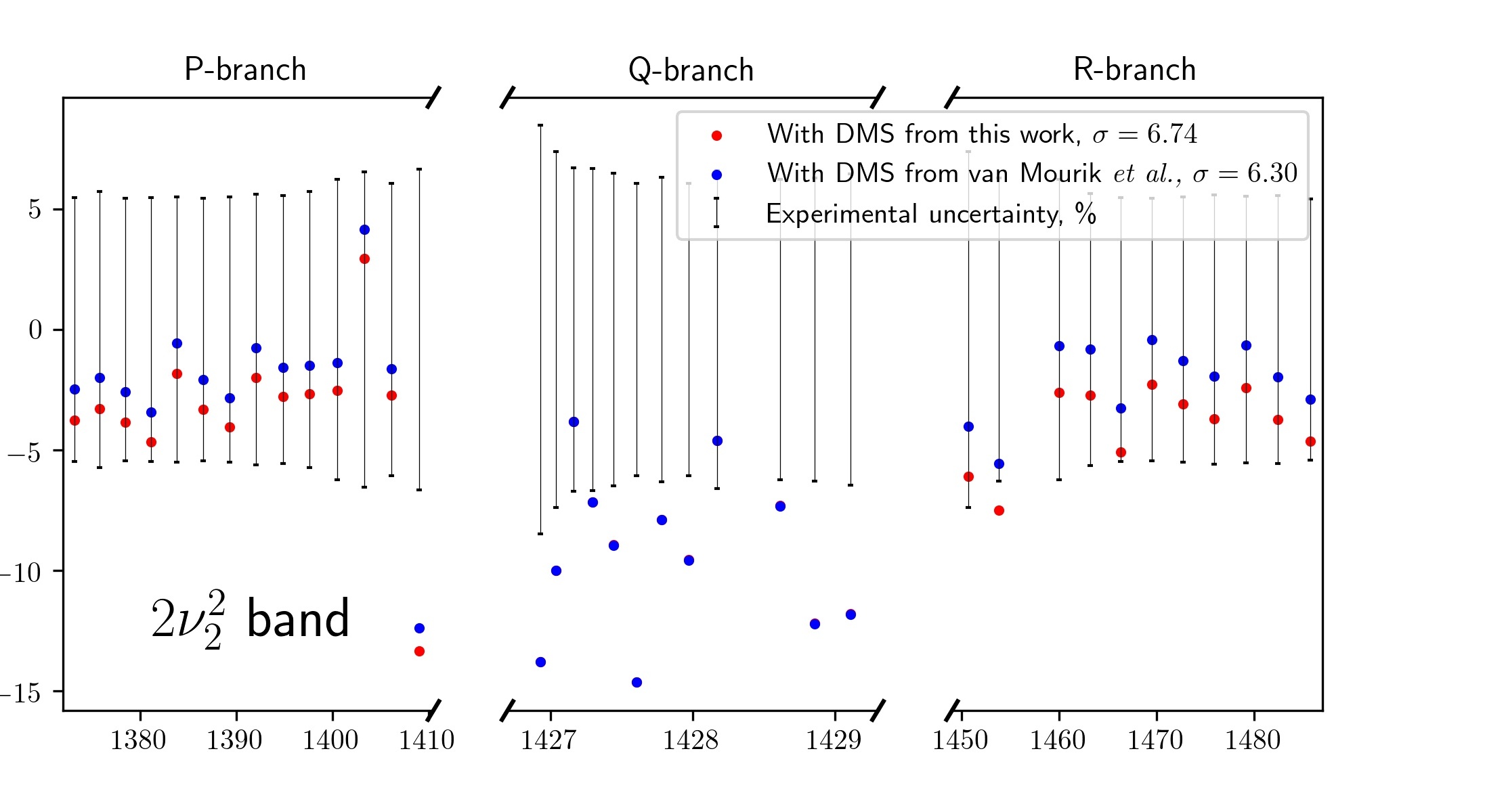
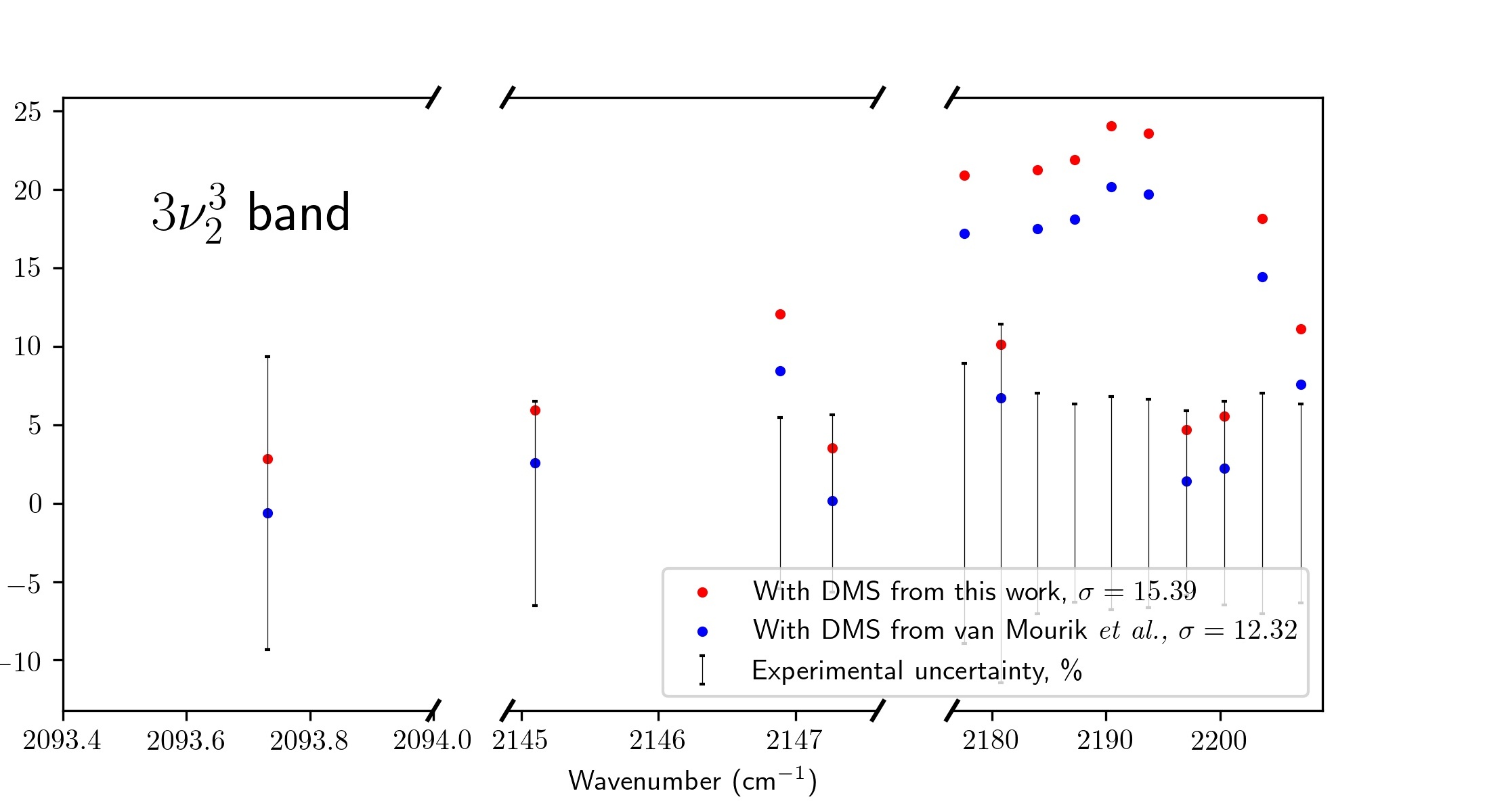
Figure 7: Comparison of line intensities for the ($0220-0000$) (upper) and ($0330-0000$) (lower) bands.

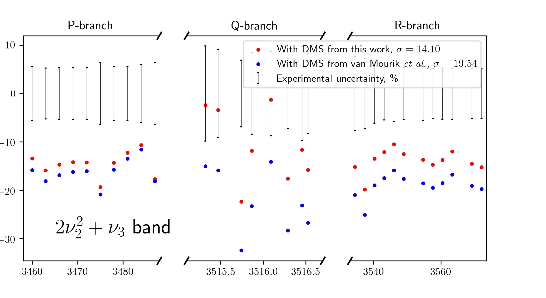
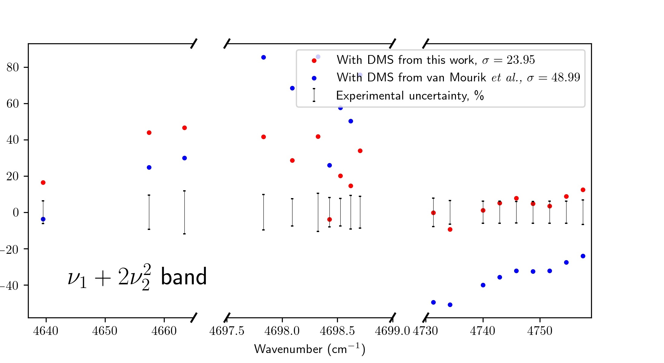
Figure 8: Comparison of line intensities for the ($0221-0000$) (upper) and ($1220-0000$) (lower) bands.

5.2.5 H¹³CN $2\nu_{1}$ (stretching H–C)

We performed calculations on the H¹³CN isotopologue to compare with the recent measurements reported by Guay et al.  [51]; a comparison is presented in table 9. Our calculations give good agreement with the observed transition intensities except for the P(20) line. Intensity difference for this line are around 12 % while for other lines the corresponding values are below 4 %. This unexpected deviation led us to analyze carefully the $2\nu_{1}$ wavenumber range.

Hebert et al.  [52] (see figure 7) studied the P-branch of H¹³CN also studied by Guay et al.  and showed that the $2\nu_{1}+\nu_{2}^{1}-\nu_{2}^{1}$ “hot” band lies in the same wavenumber range. We find that the frequency of the $2\nu_{1}+\nu_{2}^{1}-\nu_{2}^{1}$ P(9) line differs by less than 0.04 cm^-1 from the one of the $2\nu_{1}$ P(20) line. We therefore suggest that these two lines are blended meaning that the observed absorption depends on the sum of their intensities.

Table 9: Comparison of calculated H¹³CN $2\nu_{1}$ line intensities ($I$, cm/molecule, powers of 10 in parenthesis) with measurements performed at NIST [51]. Intensity difference presented as $\varepsilon=(I_{\text{calc}}/I_{\text{obs}}-1)\cdot 100~{}\%$ is performed with values obtained from ExoMol linelist [35], calculated with the “old global” DMS from [15] and the fitted PES from this work, and obtained with both new PES and DMS from this work.

Line	$I$	$\varepsilon_{\text{ExoMol}}$	$\varepsilon_{\text{olddip}}$	$\varepsilon_{\text{newdip}}$
R(8)	7.63(-23)	4	1.5	1.8
P(11)	5.97(-23)	8	4.6	4.8
P(14)	4.58(-23)	4	0.7	0.8
P(16)	3.48(-23)	1	-1.8	-1.6
P(17)	2.85(-23)	3	0.5	0.7
P(20)	1.75(-23)	-11a	-1.7a	-1.3a
P(23)	7.2(-24)	-1	-3.3	-3.2
P(24)	5.02(-24)	6	3.6	3.7
a see comments in text

6 Conclusion

In this work we present a new spectroscopically-determined potential energy surface based on a recent ab initio PES and ab initio dipole moment surface for HCN, which can be used for increased accuracy calculations of transition intensities. These data may be used in various applications such as the study of astronomical objects or intramolecular dynamics.

Spectroscopically-determined PESs are constructed for both isomers of [H,C,N] system – HCN and HNC. Experimental energy levels of hydrogen cyanide are reproduced with a standard deviation $\sigma=$0.0373 cm^-1, which is an order of magnitude better than the corresponding value for the ab initio surface. Energy levels for the significantly less harmonic hydrogen isocyanide molecule are reproduced with $\sigma=0.37$ cm^-1 compared to the ab initio value of $\sigma=4.1$ cm^-1. Differences of a few percent are obtained for many calculated transition intensities obtained using the ab initio and our new, empirical PESs. This shows the importance of high quality potentials for accurate transition intensity predictions.

A new ab initio DMS was created for HCN well to cover all transition between energy levels in 0-7200 cm^-1 range. For all fundamental transitions we compute intensities with improved agreement with the experimental data. In particular, the anomalous behaviour of the $\nu_{3}$ R-branch transitions observed by Maki et al.  [14] is described better than by previous studies.

We note that Mellau and co-workers provide energy levels which extend well beyond the 7200 cm^-1 cut-off applied here for both HCN [53, 54] and HNC [42, 43]. Attempts by us to include these levels in our separate-well treatment failed to give good results. It would be desirable to extend the accuracy of the low-energy HCN and HNC PESs and DMS to a globally accurate PES and DMS for this system. Such surfaces could be used in the subsequent production of a global accurate linelist of this system and to study behavior in the region of the saddle point between the two minima. Work in this direction is currently in progress.

References

- [1] S. T. Ridgway, D. F. Carbon, D. N. B. Hall, Polyatomic species contributing to the carbon-star 3 micron band, Astron. J. 225 (1978) 138–147. doi:10.1086/156475.
- [2] B. L. Ulich, E. K. Conklin, Detection of methyl cyanide in comet kohoutek, Nature 248 (1974) 121–122. doi:10.1038/248121a0.
- [3] K. Eriksson, B. Gustafsson, U. G. Jørgensen, A. Nordlund, Effects of HCN molecules in carbon star atmospheres, Astron. Astrophys. 132 (1984) 37–44.
- [4] S. Bruderer, D. Harsono, E. F. van Dishoeck, Ro-vibrational excitation of an organic molecule (hcn) in protoplanetary disks, Astron. Astrophys. 575 (2014) 19.
- [5] A. Tsiaras, M. Rocchetto, I. P. Waldmann, G. Tinetti, R. Varley, G. Morello, E. J. Barton, S. N. Yurchenko, J. Tennyson, Detection of an atmosphere around the super-Earth 55 Cancri e, Astrophys. J. 820 (2016) 99. doi:10.3847/0004-637X/820/2/99.
- [6] E. M. Molter, C. A. Nixon, M. A. Cordiner, J. Serigango, P. G. J. Irwin, N. A. Teanby, S. B. Charnley, J. E. Lindberg, ALMA Observations of HCN and Its Isotopologues on Titan, Astrophys. J. 152 (2016) 42.
- [7] E. S. Wirström, M. S. Lerner, P. Källström, A. Levinsson, A. Olivefors, E. Tegehall, HCN observations of comets C/2013 R1 (Lovejoy) and C/2014 Q2 (Lovejoy), Astron. Astrophys. 588 (2016) A72. doi:10.1051/0004-6361/201527482.
- [8] E. Lellouch, M. Gurwell, B. Butler, T. Fouchet, P. Lavvas, D. F. Strobel, B. Sicardy, A. Moullet, R. Moreno, D. Bockelee-Morvan, N. Biver, L. Young, D. Lis, J. Stansberry, A. Stern, H. Weaver, E. Young, X. Zhu, J. Boissier, Detection of CO and HCN in Pluto’s atmosphere with ALMA, Icarus 286 (2017) 289–307. doi:{10.1016/j.icarus.2016.10.013}.
- [9] R. J. de Kok, J. Birkby, M. Brogi, H. Schwarz, S. Albrecht, E. J. W. de Mooij, I. A. G. Snellen, Identifying new opportunities for exoplanet characterisation at high spectral resolution, Astron. Astrophys. 561 (2014) A150. doi:{10.1051/0004-6361/201322947}.
- [10] G. C. Mellau, Complete experimental rovibrational eigenenergies of HNC up to 3743 cm-1 above the ground state, J. Chem. Phys. 133 (2010) 164303. doi:{10.1063/1.3503508}.
- [11] J. H. Baraban, P. B. Changala, G. C. Mellau, J. F. Stanton, A. J. Merer, R. W. Field, Spectroscopic characterization of isomerization transition states, Science 350 (2015) 1338–1342. doi:{10.1126/science.aac9668}.
- [12] G. C. Mellau, A. A. Kyuberis, O. L. Polyansky, N. Zobov, R. W. Field, Saddle point localization of molecular wavefunctions, Sci. Rep. 6 (2016) 33068. doi:10.1038/srep33068.
- [13] R. J. Barber, G. J. Harris, J. Tennyson, Temperature dependent partition functions and equilibrium constant for HCN and HNC, J. Chem. Phys. 117 (2002) 11239–11243. doi:10.1063/1.1521131.
- [14] A. Maki, W. Quapp, S. Klee, G. C. Mellau, S. Albert, The CN mode of HCN: A comparative study of the variation of the transition dipole and Herman-Wallis constants for seven isotopomers and the influence of vibration-rotation interaction, J. Mol. Spectrosc. 174 (1995) 365–378. doi:{10.1006/jmsp.1995.0008}.
- [15] T. van Mourik, G. J. Harris, O. L. Polyansky, J. Tennyson, A. G. Császár, P. J. Knowles, Ab initio global potential, dipole, adiabatic and relativistic correction surfaces for the HCN/HNC system, J. Chem. Phys. 115 (2001) 3706–3718. doi:10.1063/1.1383586.
- [16] P. Botschwina, M. Horn, M. Matuschewski, E. Schick, P. Sebald, Hydrogen cyanide: theory and experiment, J. Molec. Struct. (THEOCHEM) 400 (1997) 119 – 137. doi:10.1016/S0166-1280(97)90273-6.
- [17] L. Lodi, J. Tennyson, Line lists for H218O and H217O based on empirically-adjusted line positions and ab initio intensities, J. Quant. Spectrosc. Radiat. Transf. 113 (2012) 850–858. doi:10.1016/j.jqsrt.2012.02.023.
- [18] M. Birk, G. Wagner, J. Loos, L. Lodi, O. L. Polyansky, A. A. Kyuberis, N. F. Zobov, J. Tennyson, Accurate line intensities for water transitions in the infrared: comparison of theory and experiment, J. Quant. Spectrosc. Radiat. Transf. 203 (2017) 88–102. doi:10.1016/j.jqsrt.2017.03.040.
- [19] E. Zak, J. Tennyson, O. L. Polyansky, L. Lodi, S. A. Tashkun, V. I. Perevalov, A room temperature CO2 line list with ab initio computed intensities, J. Quant. Spectrosc. Radiat. Transf. 177 (2016) 31–42. doi:10.1016/j.jqsrt.2015.12.022.
- [20] A. A. Kyuberis, N. F. Zobov, O. V. Naumenko, B. A. Voronin, O. L. Polyansky, L. Lodi, A. Liu, S.-M. Hu, J. Tennyson, Room temperature linelists for deuterated water, J. Quant. Spectrosc. Radiat. Transf. 203 (2017) 175–185. doi:10.1016/j.jqsrt.2017.06.026.
- [21] V. Y. Makhnev, A. A. Kyuberis, N. F. Zobov, L. Lodi, J. Tennyson, O. L. Polyansky, High accuracy ab initio calculations of rotation-vibration energy levels of the HCN/HNC system, J. Phys. Chem. A 122 (2018) 1326–1343. doi:10.1021/acs.jpca.7b10483.
- [22] S. V. Shirin, N. F. Zobov, R. I. Ovsyannikov, O. L. Polyansky, J. Tennyson, Water line lists close to experimental accuracy using a spectroscopically determined potential energy surface for H216O, H217O and H217O, J. Chem. Phys. 128 (2008) 224306.
- [23] O. L. Polyansky, R. I. Ovsyannikov, A. A. Kyuberis, L. Lodi, J. Tennyson, N. F. Zobov, Calculation of rotation-vibration energy levels of the water molecule with near-experimental accuracy based on an ab initio potential energy surface, J. Phys. Chem. A 117 (2013) 9633–9643. doi:10.1021/jp312343z.
- [24] O. L. Polyansky, R. I. Ovsyannikov, A. A. Kyuberis, L. Lodi, J. Tennyson, A. Yachmenev, S. N. Yurchenko, N. F. Zobov, Calculation of rotation-vibration energy levels of the ammonia molecule based on an ab initio potential energy surface, J. Mol. Spectrosc. 327 (2016) 21–30. doi:10.1016/j.jms.2016.08.003.
- [25] A. J. C. Varandas, S. P. . J. Rodrigues, New Double Many body expansion potential Energy Surface for Ground State HCN, J. Phys. Chem. A 110 (2006) 485–493.
- [26] A. Tajti, P. G. Szalay, A. G. Császár, M. Kállay, J. Gauss, E. F. Valeev, B. A. Flowers, J. Vázquez, J. F. Stanton, HEAT: High accuracy extrapolated ab initio thermochemistry, J. Phys. Chem. 121 (2004) 11599–11613.
- [27] A. G. Császár, W. D. Allen, H. F. Schaefer III, In pursuit of the ab initio limit for conformational energy prototypes, J. Chem. Phys. 108 (1998) 9751–9764.
- [28] A. A. Kyuberis, L. Lodi, N. F. Zobov, O. L. Polyansky, Ab initio calculation of the ro-vibrational spectrum of H2F+, J. Mol. Spectrosc. 316 (2015) 38.
- [29] G. J. Harris, O. L. Polyansky, J. Tennyson, Ab initio spectroscopy of HCN/HNC, Spectrochimica Acta A 58 (2002) 673–690. doi:10.1016/S1386-1425(01)00664-3.
- [30] G. J. Harris, O. L. Polyansky, J. Tennyson, An ab initio HCN and HNC rotation vibration linelist for astronomy, in: N. E. Piskunov, W. W. Weiss, D. F. Gray (Eds.), Modelling of stellar atmospheres, Vol. 210 of IAU Symposium, 2003.
- [31] G. J. Harris, J. Tennyson, Y. V. Pavlenko, H. R. A. Jones, Improving the quality of HCN/HNC opacity data and accounting for isotopomers, in: U. Kaufl, R. Siebenmorgen, A. Moorwood (Eds.), High Resolution Infrared Spectroscopy in Astronomy, Springer-Verlag, 2005, pp. 88–91.
- [32] G. J. Harris, J. Tennyson, B. Kaminskiy, Y. V. Pavlenko, H. R. A. Jones, Improving the Quality of HCN/HNC and H13CN data, in: F. Favata, G. A. J. Hussain, B. Battric (Eds.), Cool Stars, Stellar Systems and the Sun, Vol. 2, ESO, 2005, pp. 627–630.
- [33] G. J. Harris, J. Tennyson, B. M. Kaminsky, Y. V. Pavlenko, H. R. A. Jones, Improved HCN/HNC linelist, model atmospheres synthetic spectra for WZ Cas, Mon. Not. R. Astron. Soc. 367 (2006) 400–406.
- [34] G. J. Harris, F. C. Larner, J. Tennyson, B. M. Kaminsky, Y. V. Pavlenko, H. R. A. Jones, A H13CN/HN13C linelist, model atmospheres and synthetic spectra for carbon stars, Mon. Not. R. Astron. Soc. 390 (2008) 143–148.
- [35] R. J. Barber, J. K. Strange, C. Hill, O. L. Polyansky, G. C. Mellau, S. N. Yurchenko, J. Tennyson, ExoMol line lists – III. An improved hot rotation-vibration line list for HCN and HNC, Mon. Not. R. Astron. Soc. 437 (2014) 1828–1835. doi:10.1093/mnras/stt2011.
- [36] M. Meuwly, J. M. Hutson, Morphing ab initio potentials: A systematic study of Ne-HF, J. Chem. Phys. 110 (1999) 8338–8347. doi:{10.1063/1.478744}.
- [37] S. N. Yurchenko, M. Carvajal, P. Jensen, F. Herregodts, T. R. Huet, Potential parameters of PH3 obtained by simultaneous fitting of ab initio data and experimental vibrational band origins, Contemp. Phys. 290 (2003) 59–67.
- [38] I. I. Mizus, A. A. Kyuberis, N. F. Zobov, V. Y. Makhnev, O. L. Polyansky, J. Tennyson, High accuracy water potential energy surface for the calculation of infrared spectra, Phil. Trans. Royal Soc. London A 376 (2018) 20170149. doi:10.1098/rsta.2017.0149.
- [39] O. L. Polyansky, N. F. Zobov, I. I. Mizus, A. A. Kyuberis, L. Lodi, J. Tennyson, Potential energy surface, dipole moment surface and the intensity calculations for the 10 m, 5 m and 3 m bands of ozone, J. Quant. Spectrosc. Radiat. Transf. 210 (2018) 127–135. doi:10.1016/j.jqsrt.2018.02.018.
- [40] J. Tennyson, M. A. Kostin, P. Barletta, G. J. Harris, O. L. Polyansky, J. Ramanlal, N. F. Zobov, DVR3D: a program suite for the calculation of rotation-vibration spectra of triatomic molecules, Comput. Phys. Commun. 163 (2004) 85–116.
- [41] G. C. Mellau, Complete experimental rovibrational eigenenergies of HCN up to 6880 cm-1 above the ground state, J. Chem. Phys. 134 (2011) 234303.
- [42] G. C. Mellau, The band system of HNC, J. Mol. Spectrosc. 264 (2010) 2–9. doi:{10.1016/j.jms.2010.08.001}.
- [43] G. C. Mellau, Highly excited rovibrational states of HNC, J. Mol. Spectrosc. 269 (2011) 77–85.
- [44] L. Lodi, J. Tennyson, O. L. Polyansky, A global, high accuracy ab initio dipole moment surface for the electronic ground state of the water molecule, J. Chem. Phys. 135 (2011) 034113. doi:10.1063/1.3604934.
- [45] H.-J. Werner, P. J. Knowles, G. Knizia, F. R. Manby, M. Schütz, Molpro: a general-purpose quantum chemistry program package, WIREs Comput. Mol. Sci. 2 (2012) 242–253. doi:10.1002/wcms.82.
- [46] S. L. Hobson, E. F. Valeev, A. G. Császár, J. F. Stanton, Is the adiabatic approximation sufficient to account for the post-born-oppenheimer effects on molecular electric dipole moments?, Mol. Phys. 107 (2009) 1153–1159. doi:10.1080/00268970902780262.
- [47] V. M. Devi, D. C. Benner, M. A. H. Smith, C. P. Rinsland, S. W. Sharpe, R. L. Sams, A multispectrum analysis of the band of H12C14N: Part I. Intensities, self-broadening and self-shift coefficients, J. Quant. Spectrosc. Radiat. Transf. 82 (2003) 319 – 341, the HITRAN Molecular Spectroscopic Database: Edition of 2000 Including Updates of 2001. doi:10.1016/S0022-4073(03)00161-4.
- [48] M. A. H. Smith, C. P. Rinsland, T. A. Blake, R. Sams, D. C. Benner, V. M. Devi, Low-temperature measurements of HCN broadened by N2 in the 14- spectral region, J. Quant. Spectrosc. Radiat. Transf. 109 (2008) 922 – 951. doi:10.1016/j.jqsrt.2007.12.017.
- [49] V. M. Devi, D. C. Benner, M. A. H. Smith, C. P. Rinsland, S. W. Sharpe, R. L. Sams, A multispectrum analysis of the spectral region of H12C14N: intensities, broadening and pressure-shift coefficients, J. Quant. Spectrosc. Radiat. Transf. 87 (2004) 339 – 366. doi:10.1016/j.jqsrt.2004.03.002.
- [50] A. Maki, W. Quapp, S. Klee, G. C. Mellau, S. Albert, Intensity measurements of Delta l¿1 transitions of several isotopomers of HCN, J. Mol. Spectrosc. 185 (1997) 356–369. doi:{10.1006/jmsp.1997.7406}.
- [51] P. Guay, J. Genest, A. Fleisher, Precision spectroscopy of H13CN using a free-running, all-fiber dual electro-optic frequency comb system, J. Opt. Soc. Am. B 43 (2018) 1407–1410.
- [52] N. B. Hébert, J. Genest, J.-D. Deschênes, H. Bergeron, G. Y. Chen, C. Khurmi, D. G. Lancaster, Self-corrected chip-based dual-comb spectrometer, Opt. Express 25 (2017) 8168–8179. doi:10.1364/OE.25.008168.
- [53] G. C. Mellau, B. P. Winnewisser, M. Winnewisser, Near infrared emission spectrum of HCN, J. Mol. Spectrosc. 249 (2008) 23–42. doi:{10.1016/j.jms.2008.01.006}.
- [54] G. C. Mellau, The band system of HCN, J. Mol. Spectrosc. 269 (2011) 12–20. doi:{10.1016/j.jms.2011.04.010}.