Revisiting
Distributional Correspondence Indexing:
A Python Reimplementation and New Experiments

Abstract

This paper introduces PyDCI, a new implementation of Distributional Correspondence Indexing (DCI) written in Python. DCI is a transfer learning method for cross-domain and cross-lingual text classification for which we had provided an implementation (here called JaDCI) built on top of JaTeCS, a Java framework for text classification. PyDCI is a stand-alone version of DCI that exploits scikit-learn and the SciPy stack. We here report on new experiments that we have carried out in order to test PyDCI, and in which we use as baselines new high-performing methods that have appeared after DCI was originally proposed. These experiments show that, thanks to a few subtle ways in which we have improved DCI, PyDCI outperforms both JaDCI and the above-mentioned high-performing methods, and delivers the best known results on the two popular benchmarks on which we had tested DCI, i.e., MultiDomainSentiment (a.k.a. MDS – for cross-domain adaptation) and Webis-CLS-10 (for cross-lingual adaptation). PyDCI, together with the code allowing to replicate our experiments, is available at https://github.com/AlexMoreo/pydci .

Keywords Transfer Learning  $\cdot$ Domain Adaptation  $\cdot$ Text Classification  $\cdot$ Sentiment Classification  $\cdot$ Cross-Domain Classification  $\cdot$ Cross-Lingual Classification  $\cdot$ Python

1 Introduction

Distributional Correspondence Indexing (DCI) is a pivot-based feature-transfer domain adaptation method for cross-domain and cross-lingual text classification. DCI was first described in (Esuli and Moreo, 2015), and later improved and extended in (Moreo et al., 2016a); it was formerly implemented in Java as part of the JaTeCS (Java Text Categorization System) framework (Esuli et al., 2017), and this implementation (henceforth called JaDCI) was made publicly available.JaTeCS is a complex package, since it makes available many functionalities for text analytics research. A drawback of JaDCI is thus that, for the researcher wishing to replicate the results of (Moreo et al., 2016a) or simply wishing to use JaDCI, a substantive effort in installing and properly configuring the entire JaTeCS framework is thus needed.

In this paper we present PyDCI, a new implementation of the DCI method written in Python and built on top of the SciPy stack and scikit-learn toolkit. Python has become the preferred programming language for computer scientists. In the fields of machine learning and data mining its use has also been promoted by the appearance of Python-based environments such as SciPy and scikit-learn, whose potential and ease of use have attracted the interest of practitioners. Our reimplementation is thus in line with these trends.

With respect to JaDCI, PyDCI introduces a few modifications in the way DCI is implemented that, although subtle, bring about a significant improvement in the effectiveness of the method.

The rest of this paper is structured as follows. In Section 2 we describe the main modifications to DCI that our new implementation introduces. In Section 3 we report on new experiments that we have run using PyDCI, and show that, thanks to the modifications above, PyDCI delivers new state-of-the-art results on two popular benchmark datasets, i.e., MultiDomainSentiment (hereafter MDS – for cross-domain adaptation) and Webis-CLS-10 (for cross-lingual adaptation). These results represent a clear improvement over the ones originally obtained with JaDCI and presented in Moreo et al. (2016a), and also over the ones obtained by recent high-performing methods that have appeared Ganin et al. (2016); Li et al. (2017); Xu and Yang (2017); Zhou et al. (2016), or that we have become aware of Yang et al. (2015), after DCI was originally proposed. Section 4 concludes, hinting at future developments.

We make PyDCI publicly available via GitHub.

2 Implementation Changes

For reasons of brevity we do not re-explain DCI from scratch; we refer the interested reader to (Moreo et al., 2018) for a concise description, or to (Moreo et al., 2016a) for the full-blown presentation.

The main modifications that PyDCI introduces with respect to JaDCI are the following:

1. Document Standardization: In DCI, feature vectors and document vectors (i.e., the vectors that represent the features and the vectors that represent the documents, respectively) are post-processed via L2-normalization. In (Moreo et al., 2016a) we had witnessed improvements when applying standardization to the feature vectors (i.e., translating and scaling each dimension so that it is approximatelly normally distributed in $\mathcal{N}(0,1)$ – see (Moreo et al., 2016a, p. 144)). In PyDCI we give the user the option to apply standardization also to each dimension of the document vectors before training the classifier. All experiments we report in this paper are run with this option activated.

2. Classifier Optimization: In PyDCI we use scikit-learn’s implementation of linear SVMs (LinearSVC, which is in turn based on the liblinear package), instead of using Joachims’ SVM^light package as we had done in JaDCI. This allows us to leverage scikit-learn’s GridSearchCV utility in order to optimize SVM’s $C$ parameter (which determines the trade-off between training error and the margin) via grid search optimization, which allows us to effortlessly tune the classifier. In the new experiments using PyDCI we let parameter $C$ range in $\{10^{i}\}_{-5\leq i\leq 5}$, while in the JaDCI experiments we had simply relied on the default value that SVM^light attributes to $C$.

3. Increase in the Number of Pivots: We increase the number of pivots from 100 (the value we had used in (Moreo et al., 2016a)) to 1,000 in the cross-domain experiments and to 450 in the cross-lingual experiments. This brings about a significant improvement in performance, that does not come at a significant cost in execution time (as instead had happened with the previous implementation). We limit the number of pivots to 450 in the cross-lingual case (instead of 1,000) since in this case each pivot requires a translation to the target language which is assumed to have a cost; we thus set the number of pivots to 450 as was done in previous research (e.g., in (Prettenhofer and Stein, 2010)). We discuss below in more detail the impact on performance that the variation in the number of pivots has.

We should also mention that PyDCI relies on scikit-learn (while JaDCI relied on JaTeCS) for many preprocessing-related aspects (e.g., term weighting), which also may cause some (hard to track) differences in performance with respect to JaDCI.

3 Experiments

3.1 Effectiveness on Cross-Domain Classification and Cross-Lingual Classification

In this section we report the results we have obtained in rerunning with PyDCI the same experiments we had run with JaDCI, and whose results had been reported in (Moreo et al., 2016a). The datasets we use are arguably the most popular benchmarks in the domain adaptation literature, i.e., MDS (Blitzer et al., 2007) for cross-domain adaptation and Webis-CLS-10 (Prettenhofer and Stein, 2010) for cross-lingual adaptation. A complete description of the datasets and the standard experimental protocol followed in each case can be found either in the original publications describing the datasets (Blitzer et al., 2007; Prettenhofer and Stein, 2010) or in (Moreo et al., 2016a).

Tables 1 and 2 show the values of classification accuracy (i.e., the fraction of correctly classified documents) we obtain for cross-domain and cross-lingual classification experiments, respectively. We focus on Linear and Cosine (columns 9-10), two parameter-free probabilistic and kernel-based distributional correspondence functions (DCFs) investigated in (Moreo et al., 2016a). For each such DCF we show a direct comparison against the values we had obtained with JaDCI (Columns 7-8). We also report two baselines:

• Lower (Column 3), a classifier that directly trains on the “source” training examples and tests on the “target” unlabeled examples without performing any sort of adaptation at all. Such a classifier should thus act as a lower bound for any reasonable adaptation endeavour.

• Upper (Column 4), a classifier that trains on the “target” training examples and tests on the “target” unlabeled examples without performing any sort of adaptation at all. Such a classifier should thus act as an upper bound for any reasonable adaptation endeavour.

The baselines use exactly the same learner we use for PyDCI (LinearSVC with the $C$ parameter optimized via grid search). For each (problem, dataset) pair we also report the accuracy obtained by what, to the best of our knowledge, is today the best-performing known method on this (problem, dataset) pair (Column 5 – labelled as “SOTA”, which stands for “State Of The Art” – reports the name of the method and Column 6 reports the accuracy score, taken from the original paper). Boldface indicates the best score for each (problem, dataset) pair; shadowed cells indicate the PyDCI scores that outperform the best-known results.

Note that, aside from SDA (Glorot et al., 2011), all the baselines in the “SOTA” column had not been used as baselines in our original work on DCI; the reason is that these methods were published after DCI appeared in print (Ganin et al., 2016; Li et al., 2017; Xu and Yang, 2017; Zhou et al., 2016), or that we were unaware of them (Yang et al., 2015).

Task		Baselines		SOTA		JaDCI		PyDCI
Source	Target	Lower	Upper	method	score	Linear	Cosine	Linear	Cosine
	DVD	0.807	0.850	SDA (Glorot et al., 2011)	0.844	0.808	0.817	0.803	0.823
	Electronics	0.734	0.871	AMN (Li et al., 2017)	0.808	0.810	0.822	0.837	0.837
Books	Kitchen	0.774	0.907	DANN (Ganin et al., 2016)	0.843	0.834	0.835	0.851	0.843
	Books	0.790	0.839	DANN (Ganin et al., 2016)	0.825	0.825	0.824	0.832	0.835
	Electronics	0.757	0.871	CDFL (Yang et al., 2015)	0.809	0.822	0.824	0.839	0.855
DVD	Kitchen	0.778	0.907	DANN (Ganin et al., 2016)	0.849	0.858	0.864	0.853	0.856
	Books	0.716	0.839	AMN (Li et al., 2017)	0.780	0.766	0.764	0.796	0.800
	DVD	0.745	0.850	DANN (Ganin et al., 2016)	0.781	0.768	0.774	0.787	0.801
Electronics	Kitchen	0.859	0.907	SDA (Glorot et al., 2011)	0.902	0.864	0.868	0.871	0.878
	Books	0.737	0.839	AMN (Li et al., 2017)	0.793	0.783	0.790	0.779	0.807
	DVD	0.746	0.850	CDFL (Yang et al., 2015)	0.876	0.788	0.799	0.795	0.806
Kitchen	Electronics	0.840	0.871	SDA (Glorot et al., 2011)	0.872	0.855	0.858	0.853	0.860
	Average	0.773	0.867	AMN (Li et al., 2017)	0.814	0.815	0.820	0.825	0.833

Table 1: Cross-domain classification on the MDS dataset.

Task		Baselines		SOTA		JaDCI		PyDCI
Target Language	Domain	Lower	Upper	method	score	Linear	Cosine	Linear	Cosine
German	Books	0.523	0.863	BiDRL (Zhou et al., 2016)	0.841	0.798	0.827	0.846	0.850
	DVD	0.562	0.837	BiDRL (Zhou et al., 2016)	0.841	0.826	0.822	0.841	0.837
	Music	0.558	0.849	BiDRL (Zhou et al., 2016)	0.847	0.844	0.856	0.865	0.852
French	Books	0.558	0.844	BiDRL (Zhou et al., 2016)	0.844	0.746	0.842	0.834	0.816
	DVD	0.537	0.843	BiDRL (Zhou et al., 2016)	0.836	0.823	0.827	0.835	0.851
	Music	0.566	0.876	CLDFA (Xu and Yang, 2017)	0.833	0.816	0.844	0.824	0.842
Japanese	Books	0.498	0.802	CLDFA (Xu and Yang, 2017)	0.774	0.779	0.758	0.796	0.790
	DVD	0.500	0.814	CLDFA (Xu and Yang, 2017)	0.805	0.822	0.801	0.830	0.802
	Music	0.509	0.834	BiDRL (Zhou et al., 2016)	0.788	0.826	0.839	0.811	0.838
	Average	0.534	0.840	BiDRL (Zhou et al., 2016)	0.813	0.809	0.824	0.831	0.831

Table 2: Cross-lingual classification on the Webis-CLS-10 dataset.

PyDCI outperforms JaDCI in most cases, and outperforms also the best-performing method in the literature, which is not always the same for each (problem,dataset) pair, with very few exceptions. PyDCI obtains 7 out of 13 best results on MDS (including best averaged accuracy) when equipped with the Cosine DCF, and 5 out of 10 best results in Webis-CLS-10 when using the Linear DCF (including best averaged accuracy). In agreement with with (Moreo et al., 2016a), Cosine proved the best performing DCF, yielding the best results overall and surpassing the best accuracy obtained by any other method in 17 cases out of 23 (across the two datasets, and also including the average results). With respect to the previously best-performing system, PyDCI(Cosine) brings about a reduction in error of +10.2% on MDS and +9.6% on Webis-CLS-10.

On the very same (problem,dataset) pairs we have also run experiments in order to evaluate the impact of modifications 1 (Document Standardization) and 2 (Classifier Optimization) mentioned in Section 2. Concerning document standardization, we have rerun all the PyDCI experiments described in Tables 1 and 2 without applying document standardization. The results are reported in the first two rows of Table 3, and indicate, on average, a relative improvement in accuracy of +0.2% on MDS and +8.6% on Webis-CLS-10; document standardization thus appears to be clearly beneficial. Concerning classifier optimization, we have rerun all the PyDCI experiments described in Tables 1 and 2 without applying classifier optimization. The results are reported in the last two rows of Table 3, and indicate, on average, a relative improvement in accuracy of +9.7% on MDS and +11.8% on Webis-CLS-10; also classifier optimization is thus (unsurprisingly) clearly beneficial.

		MDS		Webis-CLS-10
Document Standardization	with	0.833	(+0.2%)	0.831	(+8.6%)
	without	0.831		0.757
Classifier Optimization	with	0.833	(+9.7%)	0.831	(+11.8%)
	without	0.767		0.743

Table 3: Average accuracy obtained using PyDCI (using the Cosine DCF) with or without document standardization and classifier optimization; percentages indicate relative improvement of the “with” configuration with respect to the corresponding “without” configuration.

3.2 Effectiveness on Cross-Domain Cross-Lingual Classification

Table 4 reports classification accuracy values obtained in the domain adaptation setting proposed in (Moreo et al., 2016a), in which both domain and language differ between the source and target (i.e., when the classification task is simultaneously cross-domain and cross-lingual). In Table 4 we include the results we had obtained in (Moreo et al., 2016a) for the Cross-Lingual Structural Correspondence Learning (SCL) method (Prettenhofer and Stein, 2010) (which we use here as a baseline), using its authors’ code (see (Prettenhofer and Stein, 2011)). The reason why we use SCL as a baseline is that, although newer approaches have been tested in this setting, none of them, to the best of our knowledge, has outperformed SCL so far.

The results in Table 4 confirm the superiority of PyDCI over JaDCI. In this case, though, the differences in performance between the “Cosine” counterparts is less pronounced. Between the PyDCI variants, Linear performs slightly better than Cosine.

Task		Baselines			JaDCI		PyDCI
Source	Target	Lower	Upper	SCL	Linear	Cosine	Linear	Cosine
EB	GD	0.495	0.837	0.784	0.790	0.827	0.834	0.812
EB	GM	0.525	0.849	0.811	0.786	0.843	0.861	0.853
EB	FD	0.533	0.843	0.780	0.810	0.823	0.841	0.832
EB	FM	0.533	0.876	0.762	0.822	0.833	0.834	0.854
EB	JD	0.491	0.814	0.742	0.813	0.805	0.830	0.816
EB	JM	0.480	0.834	0.742	0.826	0.831	0.826	0.826
ED	GB	0.568	0.863	0.823	0.823	0.824	0.855	0.808
ED	GM	0.561	0.849	0.824	0.844	0.816	0.846	0.851
ED	FB	0.511	0.844	0.790	0.744	0.848	0.839	0.828
ED	FM	0.540	0.876	0.757	0.836	0.847	0.817	0.866
ED	JB	0.505	0.802	0.725	0.738	0.761	0.775	0.769
ED	JM	0.484	0.834	0.776	0.817	0.816	0.825	0.824
EM	GB	0.536	0.863	0.825	0.791	0.812	0.811	0.846
EM	GD	0.539	0.837	0.792	0.778	0.834	0.793	0.834
EM	FB	0.523	0.844	0.784	0.810	0.845	0.816	0.812
EM	FD	0.559	0.843	0.745	0.798	0.841	0.817	0.847
EM	JB	0.503	0.802	0.708	0.711	0.721	0.785	0.746
EM	JD	0.511	0.814	0.756	0.792	0.790	0.823	0.801
	Average	0.522	0.840	0.774	0.796	0.818	0.824	0.823

Table 4: Cross-domain cross-lingual classification on the Webis-CLS-10 dataset. In the first two columns, for conciseness we use the following notation: E (English), G (German), F (French), and J (Japanese) for languages; and B (Books), D (DVD), and M (Music) for domains. E.g., GB stands for German-Books.

3.3 Statistical Significance

We have subjected our experiments to thorough statistical significance testing, by running a two-tailed t-test on paired examples across all runs (cross-domain and/or cross-lingual). The test reveals that the PyDCI versions of Linear and Cosine outperform, in a statistically significant sense, the corresponding JaDCI versions (at a confidence level of $\alpha=0.005$).

3.4 Efficiency

One important aspect of DCI in general, and of PyDCI in particular, is its efficiency. Figure 1 reports the computation times we have recorded in order to measure the efficiency of PyDCI. While the best-performing methods from the literature rely on computationally expensive optimizations (most of them are deep-learning-based), none of the experiments we have presented so far required more than 35 seconds to run.

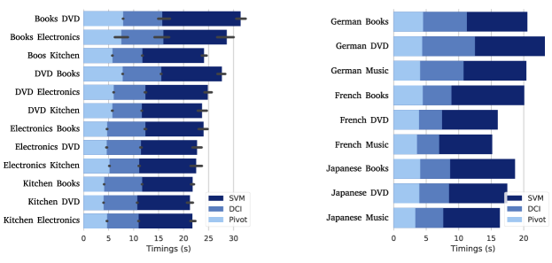
Figure 1: Computation times for the MDS (left) and Webis-CLS-10 (right) datasets. Values include the time required for pivot selection (Pivot), DCI projection (DCI), and SVM training and optimization (SVM). The time for preprocessing the documents is not included. Results for MDS are averages across 5 folds (see (Blitzer et al., 2007) for further details).

3.5 Effectiveness vs. Efficiency Trade-off

In this section we analyse the trade-off between effectiveness (in terms of classification accuracy) and time efficiency (in terms of seconds). In this experiment, we vary the number of pivots in the range $[10,25,50,100,250,500,1000,1500,2000,2500,5000]$. For the Webis-CLS-10 we bound this range to $1500$ pivots since, for some tasks it was impossible to extract more than $1500$ pivots. Figure 2 shows the average accuracy (left) and computation times for MDS and Webis-CLS-10.

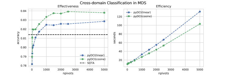
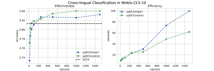
Figure 2: Effectiveness (left) and efficiency (right) of PyDCI as a function of the number of pivots, for cross-domain (top) and cross-lingual (bottom) sentiment classification.

As $npivots$ increases, PyDCI surpasses the best average accuracy reported for any other method in both datasets. In particular, and in accordance with (Moreo et al., 2016a), PyDCI equipped with the Cosine DCF does so with only 100 pivots. In this case, and in contrast with JaDCI, classification accuracy increases noticeably when more pivots are taken into account; this might be a side effect of the modifications discussed in Section 2. In any case, the method seems to reach a plateau for higher values of $npivots$, allowing the Cosine variant to reach new peaks of classification accuracy of 0.839 (when $npivots=2500$) in MDS, and 0.840 (when $npivots=1000$) in Webis-CLS-10. Regarding the efficiency of the method, PyDCI exhibits a quasi-linear trend in time complexity, e.g., when the number of pivots is doubled, the execution time is roughly doubled too.

4 Conclusions

We have presented PyDCI, a (Python-based) revision of our previous (Java-based) implementation of DCI. This new implementation incorporates changes that, although subtle, nonetheless allow the method to deliver improved results that outperform the currently known best-performing methods. The efficiency tests we have carried out speak clearly about the efficiency of PyDCI, which requires roughly half a minute to undertake any of the domain adaptation tasks in our experiments.

In a preliminary study DCI was also tested in transductive scenarios (Moreo et al., 2016b). PyDCI does not support transductive classification; this is something we plan to address in the near future.

References

- Blitzer et al. [2007] John Blitzer, Mark Dredze, and Fernando Pereira. Biographies, Bollywood, boom-boxes and blenders: Domain adaptation for sentiment classification. In Proceedings of the 45th Annual Meeting of the Association for Computational Linguistics (ACL 2007), pages 440–447, Prague, CZ, 2007.
- Esuli and Moreo [2015] Andrea Esuli and Alejandro Moreo. Distributional correspondence indexing for cross-language text categorization. In Proceedings of the 37th European Conference on Information Retrieval (ECIR 2015), pages 104–109, Wien, AT, 2015.
- Esuli et al. [2017] Andrea Esuli, Tiziano Fagni, and Alejandro Moreo. JaTeCS: An open-source Java Text Categorization System. arXiv preprint arXiv:1706.06802, 2017.
- Ganin et al. [2016] Yaroslav Ganin, Evgeniya Ustinova, Hana Ajakan, Pascal Germain, Hugo Larochelle, François Laviolette, Mario Marchand, and Victor Lempitsky. Domain-adversarial training of neural networks. The Journal of Machine Learning Research, 17(1):2096–2030, 2016.
- Glorot et al. [2011] Xavier Glorot, Antoine Bordes, and Yoshua Bengio. Domain adaptation for large-scale sentiment classification: A deep learning approach. In Proceedings of the 28th International Conference on Machine Learning (ICML 2011), pages 513–520, Bellevue, US, 2011.
- Li et al. [2017] Zheng Li, Yu Zhang, Ying Wei, Yuxiang Wu, and Qiang Yang. End-to-end adversarial memory network for cross-domain sentiment classification. In Proceedings of the 26th International Joint Conference on Artificial Intelligence (IJCAI 2017), pages 2237–2243, Melbourne, AU, 2017.
- Moreo et al. [2016a] Alejandro Moreo, Andrea Esuli, and Fabrizio Sebastiani. Distributional correspondence indexing for cross-lingual and cross-domain sentiment classification. Journal of Artificial Intelligence Research, 55:131–163, 2016a.
- Moreo et al. [2016b] Alejandro Moreo, Andrea Esuli, and Fabrizio Sebastiani. Transductive distributional correspondence indexing for cross-domain topic classification. In Proceedings of the 7th Italian Information Retrieval Workshop (IIR 2016), Venezia, IT, 2016b.
- Moreo et al. [2018] Alejandro Moreo, Andrea Esuli, and Fabrizio Sebastiani. Distributional correspondence indexing for cross-lingual and cross-domain sentiment classification (Extended Abstract). In Proceedings of the 27th International Joint Conference on Artificial Intelligence (IJCAI 2018), pages 5647–5651, Stockholm, SE, 2018. doi: 10.24963/ijcai.2018/802.
- Prettenhofer and Stein [2010] Peter Prettenhofer and Benno Stein. Cross-language text classification using structural correspondence learning. In Proceedings of the 48th Annual Meeting of the Association for Computational Linguistics (ACL 2010), pages 1118–1127, Uppsala, SE, 2010.
- Prettenhofer and Stein [2011] Peter Prettenhofer and Benno Stein. Cross-lingual adaptation using structural correspondence learning. ACM Transactions on Intelligent Systems and Technology (TIST), 3(1):13, 2011.
- Xu and Yang [2017] Ruochen Xu and Yiming Yang. Cross-lingual distillation for text classification. In Proceedings of the 55th Annual Meeting of the Association for Computational Linguistics (Volume 1: Long Papers), volume 1, pages 1415–1425, 2017.
- Yang et al. [2015] Xiaoshan Yang, Tianzhu Zhang, and Changsheng Xu. Cross-domain feature learning in multimedia. IEEE Transactions on Multimedia, 17(1):64–78, 2015.
- Zhou et al. [2016] Xinjie Zhou, Xiaojun Wan, and Jianguo Xiao. Cross-lingual sentiment classification with bilingual document representation learning. In Proceedings of the 54th Annual Meeting of the Association for Computational Linguistics (Volume 1: Long Papers), volume 1, pages 1403–1412, 2016.