Constraining Quantum Fields using Modular Theory

Nima Lashkari

School of Natural Sciences, Institute for Advanced Study,
Einstein Drive, Princeton, NJ, 08540, USA

Tomita-Takesaki modular theory provides a set of algebraic tools in quantum field theory that is suitable for the study of the information-theoretic properties of states. For every open set in spacetime and choice of two states, the modular theory defines a positive operator known as the relative modular operator that decreases monotonically under restriction to subregions. We study the consequences of this operator monotonicity inequality for correlation functions in quantum field theory. We do so by constructing a one-parameter Rényi family of information-theoretic measures from the relative modular operator that inherit monotonicity by construction and reduce to correlation functions in special cases. In the case of finite quantum systems, this Rényi family is the sandwiched Rényi divergence and we obtain a new simple proof of its monotonicity. Its monotonicity implies a class of constraints on correlation functions in quantum field theory, only a small set of which were known to us. We explore these inequalities for free fields and conformal field theory. We conjecture that the second null derivative of Rényi divergence is non-negative which is a generalization of the quantum null energy condition to the Rényi family.

1 Introduction

In recent years, the tools and techniques of quantum information theory have found many applications in many-body local quantum systems from condensed matter to field theory and gravity. In relativistic quantum field theory, studying the constraints of unitarity and causality on information-theoretic measures has led to the discovery of new inequalities that hold universally in all theories. The strong sub-additivity of entanglement entropy has been used to derive c-theorems in various dimensions [1, 2, 3]. Strong sub-additivity is a special case of the monotonicity of relative entropy which has been used to prove the average null energy condition (ANEC) in flat space and the generalized second law in curved spacetimes [4, 5]. In this work, we explore a large class of monotonicity constraints of information-theoretic measures in quantum field theory.

In quantum field theory, there are no density matrices associated to finite regions of spacetime. This is an obstacle on the way of applying the entanglement theory to quantum fields which reflects itself as ultraviolet divergences that appear in entanglement entropy. In some cases, one can use scaling arguments to isolate universal pieces in the calculations. These ultraviolet divergences point to the fact that entanglement in quantum field theory is a property of the algebra and not the states [6].

A more satisfactory approach is provided by the Tomita-Takesaki modular theory that studied the algebra of local operators in quantum field theory; see [7, 6] for a review. Modular theory connects with information theory by defining a positive operator known as the relative modular operator. Araki realized that the expectation value of the logarithm of this operator generalizes the density matrix definition of relative entropy to arbitrary quantum systems including quantum field theory [8]. Relative entropy is a distance measure central to quantum information theory from which most other entanglement measures can be derived; see [9] for a review.

In modular theory, the relative modular operator $\Delta^{A}_{\Omega|\Phi}$ is defined for every spacetime region $A$ and choice of two states $|\Omega\rangle$ and $|\Phi\rangle$. The locality of quantum field theory imposes a strong constraint on how the relative modular operator changes as one changes the region $A$. Most importantly for us, the relative modular operator is monotonic, that is to say for any region $A\subset B$ we have

$$\Delta^{A}_{\Omega|\Phi}\geq\Delta^{B}_{\Omega|\Phi}$$ (1)

as an operator inequality. It implies the monotonicity of relative entropy, however, as an operator inequality, it is much stronger. In this work, we study the consequences of this inequality in quantum field theory.

In section 2, we review the modular theory emphasizing those properties of the relative modular operator that play an important role in our work. In section 3, we introduce the Petz divergence as an information-theoretic measure that monotonically increases as one enlarges the region, and show that it satisfies all the desirable information-theoretic properties one expects from a Rényi generalization of relative entropy. In section 4, motivated by the work of Araki and Masuda in [10] we define an alternative Rényi family for relative entropy and show that it is the generalization of the sandwiched Rényi divergence to quantum field theory. Similar discussions appear in [11, 12, 13]. Our approach has the advantage that we do not need to resort to the proofs in [14, 15, 13] to show the monotonicity of sandwiched Rényi divergences. It is implied by the monotonicity of relative modular operator. For completeness, we review of the proof of the monotonicity of relative modular operator with an emphasis on finite dimensional Hilbert spaces in section 5.

In [16] a Euclidean path-integral was constructed that computes sandwiched Rényi divergences, and it was shown that for certain values of the Rényi index they are given by correlation functions. Section 6 starts with this path-integral construction and explores the consequences of monotonicity for these correlation functions. We find new inequalities that the $2n$-point correlation functions have to satisfy as a consequence of monotonicity. They can be interpreted as the non-negativity of certain off-diagonal elements of null momentum. See the inequality in (84) for a concrete example.

Studying the dependence of these $2n$-point correlation functions on the region size we are naturally led to the conjecture that the second null (or spacelike) derivatives of the sandwiched Rényi divergence is non-negative. This can be thought of as a generalization of quantum null energy condition to the Rényi family. We provide evidence for the conjecture using reflection positivity of Euclidean correlators. We perform sample calculations of the sandwiched Rényi divergence and its derivatives in shape deformations in free two-dimensional bosons and higher-dimensional conformal field theories in a local quench limit.

Finally, we conclude in section 7 by discussing generalizations and comment on potential implications of our work for constraining bulk effective field theories in holography.

2 Tomita-Takesaki modular theory

A general quantum system is described by an algebra of bounded operators with a $\dagger$ operation and a notion of a norm. In this abstract language, states are linear maps from the algebra to correlation functions. Given a state, there is a well-defined prescription to construct an irreducible representation of such an algebra in the Hilbert space. If the algebra is generated by operators that satisfy the canonical commutation relation Lie algebra then such an irreducible representation is unique up to unitary equivalence. This is not the case in quantum field theory. There are many inequivalent representations of the algebra of operators in the Hilbert space that correspond to different superselection sectors. This is one of the main motivations to study the local algebra of operators in quantum field theory.

The algebra of local operators in quantum field theory differs from finite dimensional quantum systems in essential ways. Given a state living on a Cauchy slice, there is no notion of density matrix operator corresponding to a subregion. This causes a problem for a naive generalization of entanglement theory from finite quantum systems to field theory. The Tomita-Takesaki modular theory allows us to define information-theoretic measures in quantum field theory without the need to define density matrices.

Consider a relativistic quantum field theory in Minkowski space in $D$ spacetime dimensions. For every open set $A$ in spacetime, there exists a von Neumann algebra of bounded operators $\mathcal{A}_{A}$ that is generated by bounded functions of fundamental fields integrated against test functions supported on $A$. Locality requires that $\mathcal{A}_{B}\subset\mathcal{A}_{A}$ if $B\subset A$. The closure of the union of algebras associated with all open sets forms the global algebra of quantum field theory. In a relativistic quantum field theory, a Poincaré transformation that sends $A\to\Lambda(A)$ corresponds to an automorphism of the global algebra that transforms $\mathcal{A}\to\mathcal{A}_{\Lambda(A)}$. We think of states on $A$ as linear maps $\omega_{A}$ from the local algebra $\mathcal{A}_{A}$ to expectation values, and denote the states of the global algebra with vectors $|\Omega\rangle$ in the Hilbert space.

Every von Neumann algebra $\mathcal{A}_{A}$ has a notion of $\dagger$. Therefore, for any two vectors $|\Omega\rangle$ and $|\Phi\rangle$ and a region $A$ one can define the relative Tomita operator by its action

$$S^{A}_{\Phi|\Omega}a|\Omega\rangle=a^{\dagger}|\Phi\rangle,$$ (2)

where $a$ is an operators in the algebra $\mathcal{A}_{A}$ of region $A$, and $|\Omega\rangle$ is carefully chosen such that $a|\Omega\rangle$ and $a^{\prime}|\Omega\rangle$ are dense in the Hilbert space. We further assume that there exists no $a\in\mathcal{A}$ such that $a|\Omega\rangle=0$. Such states are called cyclic and separating. The definition in (2) can be extended to arbitrary vectors, however, to simplify the presentation we restrict our discussion to vectors that are cyclic and separating.

The relative modular operator $\Delta_{\Phi|\Omega}$ is the norm of the relative Tomita operator:

$$\Delta_{\Phi|\Omega}\equiv S^{\dagger}_{\Phi|\Omega}S_{\Phi|\Omega}\ .$$ (3)

It is unbounded and manifestly non-negative. From the definition of the Tomita operator it is clear that

$$S_{\Phi|\Omega}S_{\Omega|\Phi}=1,\qquad S_{\Phi|\Omega}^{\dagger}S_{\Omega|\Phi}^{\dagger}=1,$$ (4)

hence the action of $\Delta^{-1}_{\Omega|\Phi}=S_{\Phi|\Omega}S_{\Phi|\Omega}^{\dagger}$. Furthermore, the Tomita operator for region $A$ is the Hermitian conjugate of that of $A^{\prime}$ (its causal complement): $(S^{A}_{\Phi|\Omega})^{\dagger}=S^{A^{\prime}}_{\Phi|\Omega}$ [17]. As a result, the relative modular operators $(\Delta^{A}_{\Omega|\Phi})^{-1}=\Delta^{A^{\prime}}_{\Phi|\Omega}$. This operator plays an important role in our discussion. Most importantly for us, the relative modular operator for any two vectors $|\Phi\rangle$ and $|\Omega\rangle$ satisfies the monotonicity inequality

$$\Delta^{B}_{\Omega|\Phi}\leq\Delta^{A}_{\Omega|\Phi}$$ (5)

for any $\mathcal{A}_{A}\subset\mathcal{A}_{B}$. This is a consequence of the fact that the domain of $S^{B}_{\Phi|\Omega}$ is an extension of that of $S^{A}_{\Phi|\Omega}$. That is to say for any $a\in\mathcal{A}_{A}$ we have

$$S^{A}_{\Omega|\Phi}a|\Phi\rangle=S^{B}_{\Omega|\Phi}a|\Phi\rangle=a^{\dagger}|\Omega\rangle\ .$$ (6)

This implies that for vectors $a|\Phi\rangle$ with $a\in\mathcal{A}_{A}$ the monotonicity of the relative modular operator is saturated:

$$\langle\Phi|a^{\dagger}\Delta^{A}_{\Omega|\Phi}a|\Phi\rangle=\langle\Phi|a^{\dagger}\Delta^{B}_{\Omega|\Phi}a|\Phi\rangle\ .$$ (7)

To obtain an inequality we consider non-linear functions of $\Delta_{\Omega|\Phi}$ that inherit monotonicity by construction. A function $f:(0,\infty)\to(0,\infty)$ is called operator monotone if for any self-adjoint operators $X\geq Y\geq 0$ we have $f(X)\geq f(Y)\geq 0$. An important example is $f(z)=z^{\alpha}$ which is operator monotone for for $0<\alpha<1$ [6]. For invertible operators, $X>Y>0$ implies $Y^{-1}>X^{-1}$. The relative modular operator is invertible, therefore it satisfies the monotonicity operator inequality

$$\operatorname{sign}(\alpha)(\Delta^{A}_{\Omega|\Phi})^{-\alpha}\leq\operatorname{sign}(\alpha)(\Delta^{B}_{\Omega|\Phi})^{-\alpha}$$ (8)

for $1\geq\alpha\geq-1$. Another important operator monotone function is the principal branch logarithm on positive definite operators which implies that Araki’s relative entropy

$$S(\Phi\|\Omega)=-\langle\Phi|\log\Delta_{\Omega|\Phi}|\Phi\rangle$$ (9)

is monotonic. In this work, we mostly focus on $f(z)=z^{\alpha}$ and briefly comment on other operator monotone functions until section 7.

To study the entanglement between region $A$ and $A^{\prime}$ it is natural to focus on quantities that are independent of unitaries in the region $A$ and $A^{\prime}$. Hence, we should understand how the relative modular operator transforms when the vectors are rotated by unitaries in $A$ and $A^{\prime}$. One can check directly from the definition in (2) that $S_{UU^{\prime}\Omega|VV^{\prime}\Psi}=VU^{\prime}S_{\Omega|\Psi}V^{\prime\dagger}U^{\dagger}$ satisfies

$$S_{UU^{\prime}\Omega|VV^{\prime}\Psi}aVV^{\prime}|\Psi\rangle=a^{\dagger}UU^{\prime}|\Omega\rangle$$ (10)

for unitaries $U,V\in\mathcal{A}_{A}$ and $U^{\prime},V^{\prime}\in\mathcal{A}_{A^{\prime}}$. As a result, the relative modular operator transforms according to

$$\Delta_{UU^{\prime}\Omega|VV^{\prime}\Psi}=UV^{\prime}\Delta_{\Omega|\Psi}V^{\prime\dagger}U^{\dagger}\ .$$ (11)

This transformation rule plays an important in section 3 when we engineer information-theoretic quantities from the relative modular operator that are invariant under local unitaries.

In a quantum field theory with a stress tensor, shape deformations are generated by unitaries that are exponentiated integrals of the stress tensor. Consider a diffeomorphism that deforms region $A$ continuously to its subregion $B$ and represent it by unitary $U$. In this work, we consider only the shape deformations that leave the vacuum invariant:

$$\mathcal{A}_{A}=U\mathcal{A}_{B}U^{\dagger},\qquad U|\Omega\rangle=|\Omega\rangle\ .$$ (12)

Examples of such unitaries are Poincare transformations and arbitrary deformations on null hypersurfaces. The reason is that for such unitaries, we can explicitly relate the relative modular operator of $B$ with that of $A$ using the definition of the relative Tomita operator:

$$S^{B}_{\Psi|\Omega}a_{B}|\Omega\rangle=(U^{\dagger}S^{A}_{U\Psi|\Omega}U)a_{B}|\Omega\rangle$$ (13)

and

$$\Delta^{B}_{\Psi|\Omega}=U^{\dagger}\Delta^{A}_{U\Psi|\Omega}U\ .$$ (14)

In the limit the size of region $A$ shrinks to zero the state $|\Phi\rangle$ and $|\Omega\rangle$ are indistinguishable, therefore one expects the matrix elements of $f(\Delta_{\Omega|\Phi})$ to converge to those of $f(\Delta_{\Phi})$. In particular, this implies that for any operator monotone function $f$ and any region $A$ we have

$$\langle\Phi|f(\Delta^{A}_{\Omega|\Phi})|\Phi\rangle-f(1)\leq 0\ .$$ (15)

We are now ready to construct information-theoretic measures out of the relative modular operator. The class of measures that we will show to be related to the quantum field theory correlation functions is called the sandwiched Rényi divergence. In the next section, we start by a closely related but simpler class of measures called Petz divergences.

3 Petz divergences

The monotonicity of relative entropy in (8) is an operator equation which implies

$$\operatorname{sign}(\alpha)\langle\Psi|(\Delta^{A}_{\Omega|\Phi})^{-\alpha}|\Psi\rangle\leq\operatorname{sign}(\alpha)\langle\Psi|(\Delta^{B}_{\Omega|\Phi})^{-\alpha}|\Psi\rangle$$ (16)

for any $A\subset B$, $\alpha\in[-1,1]$ and any vector $|\Psi\rangle$ in the Hilbert space. The matrix element $\langle\Psi|(\Delta^{A}_{\Omega|\Phi})^{-\alpha}|\Psi\rangle$ depends on the information in both $A$ and the complementary region $A^{\prime}$. In entanglement theory we are interested in “semilocal” quantities, meaning those that are independent of the information content in $A^{\prime}$. If $|\Phi\rangle$ is cyclic and separating the vector $a|\Phi\rangle$ with $a\in\mathcal{A}$ is dense in the Hilbert space, therefore it is natural to consider Petz quasi-entropies introduced in [20]

$$D^{A}_{\alpha,a}(\Phi\|\Omega)=\frac{1}{\alpha}\log\langle\Phi|a^{\dagger}(\Delta^{A}_{\Omega|\Phi})^{-\alpha}a|\Phi\rangle\ .$$ (17)

where the operator $a$ is normalized such that $\langle\Omega|a^{\dagger}a|\Omega\rangle=1$ and $\alpha\in[-1,1]$ . This normalization makes sure quasi-entropies vanish at $\alpha=-1$ because

$$\langle\Phi|a^{\dagger}(\Delta^{A}_{\Omega|\Phi})a|\Phi\rangle=\langle\Omega|a^{\dagger}a|\Omega\rangle=1\ .$$ (18)

Under unitary rotations in $A^{\prime}$ the relative modular operator transforms according to (11), and since $[a,U^{\prime}]=0$ the Petz quasi-entropy remains invariant.

In addition, this Rényi family has the following properties:

1. If $A\subset B$ and $a\in\mathcal{A}_{A}$ then it increases monotonically with system size:

   $$D^{A}_{\alpha,a}(\Phi\|\Omega)\leq D^{B}_{\alpha,a}(\Phi\|\Omega).$$

2. If $U$ is a unitary in $\mathcal{A}_{A}$ then $D_{\alpha,a}^{A}(U\Phi\|V\Omega)=D_{\alpha,V^{\dagger}aU}^{A}(\Phi\|\Omega)$.

3. It increases monotonically in $\alpha$. If $\alpha\leq\beta$ then $D^{A}_{\alpha,a}(\Phi\|\Omega)\leq D^{A}_{\beta,a}(\Phi\|\Omega)$.

See appendix A for a proof. In the remainder of this work, we focus on quasi-entropies in the case $a=1$, where the subregion monotonicity property extends to all subregions. For $a=1$, we have the Petz divergence:

$$D_{\alpha}(\Phi\|\Omega)=\frac{1}{\alpha}\log\langle\Phi|\Delta^{-\alpha}_{\Omega|\Phi}|\Phi\rangle$$ (19)

with the following additional properties:

1. It is non-negative and vanishes when $A$ shrinks to zero.

2. It is invariant under the rotation of both vectors by the same unitary in $A$.

3. At $\alpha=0$ it is smooth and equal to the relative entropy.

4. Under swapping vectors $|\Phi\rangle$ and $|\Omega\rangle$ it satisfies

   $$D_{-\alpha}(\Phi\|\Omega)=\frac{1-\alpha}{\alpha}\>D_{\alpha-1}(\Omega\|\Phi)\ .$$ (20)

See appendix B for proofs.

Petz divergences vanish at $\alpha=-1$ and increase monotonically in $\alpha$. They acquire their maximum at $\alpha=1$:

$$D_{1}(\Phi\|\Omega)=\log\langle\Phi|\Delta_{\Omega|\Phi}^{-1}|\Phi\rangle=\log\langle\Omega|S^{\dagger}_{\Phi|\Omega}(S_{\Phi|\Omega}S_{\Phi|\Omega}^{\dagger})S_{\Phi|\Omega}|\Omega\rangle=\log\langle\Omega|\Delta^{2}_{\Phi|\Omega}|\Omega\rangle\ .$$ (21)

If $|\Phi\rangle\sim\Phi^{\prime}|\Omega\rangle$ with $\Phi^{\prime}\in\mathcal{A}^{\prime}$ since $(S^{A}_{\Phi|\Omega})^{\dagger}$ is an extension of $S^{A^{\prime}}_{\Phi|\Omega}$ we have

$$D_{1}(\Phi\|\Omega)=\log\left(\frac{\langle\Omega||\Phi^{\prime}|^{4}|\Omega\rangle}{\langle\Omega||\Phi^{\prime}|^{2}|\Omega\rangle^{2}}\right)\ .$$ (22)

4 Sandwiched Rényi divergences

The Petz divergence satisfies all the desired properties an information-theorist would want, however it cannot be written in terms of the correlation functions of quantum field theory in a simple way. A closely related monotonic Rényi family called the sandwiched Rényi divergence was introduced in [21, 22] for finite quantum systems. In [16] it was shown that for special values of $\alpha$, in quantum field theory, the sandwiched Rényi divergences can be written in terms of correlation functions. We focus on this new family in this section.

To motivate an algebraic definition of the sandwiched Rényi divergence we follow the approach in [10]. Consider a vector $|\Phi\rangle$ that is in the intersection of the domain of $\Delta_{\Omega|\Psi}^{-1}$ for all $|\Psi\rangle\in\mathcal{H}$. We define the sandwiched Rényi divergence to be

$$S^{A}_{\alpha}(\Phi\|\Omega)\equiv\frac{1}{\alpha}\sup_{|\Psi\rangle\in\mathcal{H}}\log\langle\Phi|(\Delta_{\Omega|\Psi}^{A})^{-\alpha}|\Phi\rangle$$

$$S^{A}_{-\alpha}(\Phi\|\Omega)\equiv\frac{-1}{\alpha}\inf_{|\Psi\rangle\in\mathcal{H}}\log\langle\Phi|(\Delta_{\Omega|\Psi}^{A})^{\alpha}|\Phi\rangle$$ (23)

for $0\leq\alpha<1$. If the intersection of the domains of $\Delta_{\Omega|\Psi}^{-1}$ for all $|\Psi\rangle$ does not include $|\Phi\rangle$ the Sandwiched Rényi divergence is defined to be infinite. However, we will show that it is finite for a dense set of states $\Phi^{\prime}|\Omega\rangle$ where $\Phi^{\prime}$ is an operator in the commutant. Sandwiched Rényi divergences satisfy all the desired properties that led us to Petz divergences. The subregion monotonicity and non-negativity are inherited from (16) by definition. The monotonicity in $\alpha$ follows from Holder’s inequality similar to the argument presented in appendix B. It is also invariant under rotation by untiaries in $A^{\prime}$, and under unitary rotations in $A$, it transforms according to $S_{\alpha}(V\Phi\|U\Omega)=S_{\alpha}(U^{\dagger}V\Phi\|\Omega)=S_{\alpha}(\Phi\|V^{\dagger}U\Omega)$. Similar to the Petz entropy it vanishes when the two vectors are the same, but as opposed to the Petz entropy, it does not vanish at $\alpha=-1$. In fact, its value at $\alpha=-1$ is related to an important distance measure called quantum fidelity.

From the definition (4) it is clear that sandwich Rényi divergences are larger than their cousins:

$$S_{\alpha}(\Phi\|\Omega)\geq D_{\alpha}(\Phi\|\Omega)\ .$$ (24)

An analogy with finite dimensional quantum systems helps to unpack the definition in (4). This definition is based on a generalization of the notion of the $p$-norm of a matrix to unbounded operators [10]. Remember that for a matrix $X$ the $p$-norm is defined to be $\|X\|_{p}=tr(|X|^{p})^{1/p}$. It is invariant under unitary rotations, $\|X\|_{p}=\|U^{\dagger}XU\|_{p}$, and it satisfies the Holder inequality

$$\|XY\|_{1}\leq\|X\|_{p}\|Y\|_{q}$$

for any $p,q>1$ with $p^{-1}+q^{-1}=1$. By the definition of the norm $|tr(XC)|\leq\|XC\|_{1}$ for any operator $C$. As a result,

$$\sup_{\|C\|_{q}=1}|tr(XC)|\leq\sup_{\|C\|_{q}=1}\|XC\|_{1}\leq\|X\|_{p}$$ (25)

where in the second step we have used Holder’s inequality. If we pick $C$ proportional to $|X|^{p/q}U^{\dagger}$ where $X=U|X|$ is the polar decomposition of $X$ and the overall factor of $C$ is fixed such that $\|C\|_{q}=1$, we find that the inequality above is saturated. In other words, we have the norm duality relation

$$\|X\|_{p}=\sup_{\|C\|_{q}=1}|tr(XC)|\ .$$ (26)

Our operators of interest are not trace class, however, choosing a reference state $|\Omega\rangle$ and an algebra of region $A$ following Araki and Masuda [10] one can still define the $p$-norm of a vector $|\Phi\rangle$ using the definition

$$p\in[2,\infty]\qquad\||\Phi\rangle\|^{A}_{p,\Omega}=\sup_{|\Psi\rangle}\|\Delta_{\Psi|\Omega}^{1/2-1/p}|\Phi\rangle\|$$

$$p\in[1,2)\qquad\||\Phi\rangle\|^{A}_{p,\Omega}=\inf_{|\Psi\rangle}\|\Delta_{\Psi|\Omega}^{1/2-1/p}|\Phi\rangle\|\ .$$ (27)

As we discussed in section 2, we know that $(\Delta^{A}_{\Omega|\Psi})^{-1}=\Delta^{A^{\prime}}_{\Psi|\Omega}$, therefore the sandwiched Rényi divergence can be written as

$$S^{A}_{\alpha}(\Phi\|\Omega)=\frac{2}{\alpha}\log\||\Phi\rangle\|^{A^{\prime}}_{\frac{2}{1-\alpha},\Omega}\ .$$ (28)

The reason for switching from supremum to infimum as we go from positive to negative values of $\alpha$ is a generalization of (26) to the norms defined in (4) that relates the $p$ and $q$ norms when $\frac{1}{p}+\frac{1}{q}=1$. To see this, consider the Cauchy-Schwarz inequality

$$\frac{|\langle\Phi|\chi\rangle|}{\langle\Phi|\Delta_{\Omega|\Psi}^{-\alpha}|\Phi\rangle^{1/2}}\leq\langle\chi|\Delta_{\Omega|\Psi}^{\alpha}|\chi\rangle^{1/2}\ .$$ (29)

Taking the infimum over $|\Psi\rangle$ we have

$$\inf_{|\Psi\rangle}\frac{|\langle\Phi|\chi\rangle|}{\langle\Phi|\Delta_{\Omega|\Psi}^{-\alpha}|\Phi\rangle^{1/2}}\leq\inf_{|\Psi\rangle}\langle\chi|\Delta_{\Omega|\Psi}^{\alpha}|\chi\rangle^{1/2}\ .$$

In fact, the supremum of the left-hand-side over all vectors $|\Phi\rangle$ saturates the inequality [10]

$$\sup_{|\Phi\rangle}\frac{|\langle\Phi|\chi\rangle|}{\sup_{|\Psi\rangle}\langle\Phi|\Delta_{\Omega|\Psi}^{-\alpha}|\Phi\rangle^{1/2}}=\inf_{|\Psi\rangle}\langle\chi|\Delta_{\Omega|\Psi}^{\alpha}|\chi\rangle^{1/2}\ .$$ (30)

As a result, we have the norm duality relation

$$\sup_{\||\Phi\rangle\|_{p,\Omega}=1}|\langle\Phi|\chi\rangle|=\||\chi\rangle\|_{q,\Omega}\ .$$ (31)

This is a generalization of (26) to von Neumann algebras.

For special values of $\alpha$ the sandwiched Rényi divergences in (4) is of particular interest in information theory:

• $\alpha=1$: Due to the monotonicity in $\alpha$, this is the maximum of the sandwiched Rényi divergence in $\alpha$ and it is given by the norm of the operator that creates the state. If $|\Phi\rangle=\Phi^{\prime}|\Omega\rangle$ we have

  $$S_{1}(\Phi\|\Omega) = \sup_{|\Psi\rangle}\log\langle\Phi|\Delta_{\Omega|\Psi}^{-1}|\Phi\rangle=\sup_{|\Psi\rangle}\log\langle\Phi|S_{\Psi|\Omega}S_{\Psi|\Omega}^{\dagger}|\Phi\rangle$$

  $$= \sup_{|\Psi\rangle}\log\langle\Psi|\|\Phi^{\prime}\|^{2}|\Psi\rangle=2\log\|\Phi^{\prime}\|$$

  where we have used $(S^{A}_{\Psi|\Omega})^{\dagger}=S^{A^{\prime}}_{\Psi|\Omega}$. An important implication of this result is that for states $\Phi^{\prime}|\Omega\rangle$ with $\Phi^{\prime}$ bounded all the sandwiched Renyi divergences are finite and free of ultraviolet divergences. This is a dense set of states. Haag and Swieca have argued that the norm of the operator that creates the state should be interpreted as a measure of how localized the state is [23]. Smaller $S_{1}(\Phi\|\Omega)$ corresponds to a state more localized in $A^{\prime}$. A unitary $U^{\prime}$ creates an excitation completely localized in $A^{\prime}$.

• $\alpha=\frac{1}{2}$: This value corresponds to a generalization of “collision entropy” to von Neumann algebras: $S_{\frac{1}{2}}(\Phi\|\Omega)=2\sup_{\Psi}\langle\Phi|\Delta_{\Omega|\Psi}^{-1/2}|\Phi\rangle$. As we will see in the next section, this value of $\alpha$ can be related to Euclidean four point functions.

• $\alpha=0$: Similar to the Petz divergence the sandwiched divergences is equal to the relative entropy at $\alpha=0$. To see this, we show the following inequality in appendix C:

  $$D_{\frac{\alpha}{1-\alpha}}(\Phi\|\Omega)\geq S_{\alpha}(\Phi\|\Omega)\geq D_{\alpha}(\Phi\|\Omega)\ .$$ (32)

  In the limit $\alpha\to 0$ the sandwiched Rényi divergence is upper and lower bounded by relative entropy.

• $\alpha=-1$: This value of $\alpha$ provides a generalization of “quantum Fidelity” to von Neumann algebras:

  $$S_{-1}(\Phi\|\Omega)=-2\log F(\Phi,\Omega)$$

  $$F(\Phi,\Omega)\equiv\||\Phi\rangle\|_{1,\Omega}^{A^{\prime}}$$ (33)

  In the next section, we will show that for density matrices $F(\Phi,\Omega)$ reduces to the standard expression for quantum Fidelity. From norm duality we know that Fidelity as defined above is the supremum over overlaps $\langle\Psi|\Phi\rangle$ for $|\Psi\rangle=\Psi^{\prime}|\Omega\rangle$ and $\|\Psi^{\prime}\|=1$:

  $$F(\Phi,\Omega)=\sup_{\||\chi\rangle\|_{\infty,\Omega}^{A^{\prime}}=1}|\langle\chi|\Phi\rangle|\ .$$ (34)

  This is the analogue of Uhlemann’s theorem in quantum field theory [24].

5 Finite-dimensional Quantum Systems

Up to here, the discussion of the relative modular operator and our information-theoretic measures applied to any quantum system from qubits to quantum field theory. To come in contact with the information theory literature, in this section, we write our measures for finite quantum systems in terms of density matrices, and provide a simple proof of the monotonicity of the Petz divergence and the sandwiched Rényi divergence. We closely follow the arguments presented in [19] and [6]; see also [25] for a similar proof. Consider a bipartite quantum system described by a density matrix $\sigma_{12}$ and its reduced density matrix on the first subsystem $\sigma_{1}$. It is convenient to purify $\sigma_{12}$ in a pure state of a four-partite system

$$|\Omega\rangle=\sum_{i,j=1}^{d}c_{ij}|ij,ij\rangle\in\mathcal{H}$$ (35)

where $|ij\rangle$ are the eigenvectors of $\sigma_{ij}$ and we have assumed that the local Hilbert at each site is $d$-dimensional. In our notation, we separate the indices corresponding to the Hilbert space of the system from those of the purification by a comma. The coefficients $c_{ij}$ are the Schmidt coefficients of $|\Omega\rangle$ and the square root of eigenvalues of $\sigma_{12}$. For simplicity, we assume that $\sigma_{12}$ is full-rank which implies that all $c_{ij}>0$. Similarly, we purify $\sigma_{1}$ in a bi-partite pure state

$$|\omega\rangle=\sum_{i}d_{i}|i,i\rangle\in\mathcal{K}$$

$$d_{i}^{2}=\sum_{j}c^{2}_{ij}.$$ (36)

The local algebra on each site is the algebra of $d\times d$ complex matrices with its natural notion of $\dagger$ and norm. We consider the algebras $\mathcal{A}=\mathcal{A}_{1}$ and $\mathcal{B}=\mathcal{A}_{1}\otimes\mathcal{A}_{2}$ that are generated by $a_{ik}=|i\rangle\langle k|$ and $b_{ijkl}=|ij\rangle\langle kl|$, respectively. Acting on the state $|\Omega\rangle$ with $b\in\mathcal{B}$ we can obtain arbitrary states $\mathcal{H}$. Similarly, any state in $\mathcal{K}$ can be written as $a|\omega\rangle$ with $a\in\mathcal{A}$.

The state $|\omega\rangle$ can be though of as

$$|\omega\rangle=\sigma_{1}^{1/2}|E_{\omega}\rangle$$

$$|E_{\omega}\rangle=\sum_{j}|j,j\rangle$$ (37)

where $|E_{\omega}\rangle$ is an unnormalized maximally entangled state in the basis spanned by $|j\rangle$, the eigenvectors of $\sigma_{1}$ [26]. Note that for any full rank density matrix $\sigma$ we have

$$\langle\omega|X\otimes Y|\omega\rangle=\langle E_{\omega}|\sigma^{1/2}X\sigma^{1/2}\otimes Y|E_{\omega}\rangle=tr(\sigma^{1/2}X\sigma^{1/2}Y)\ .$$ (38)

Consider the state $|\omega\rangle$ on systems $13$ tensored with another copy of it on $24$: $|\omega\rangle_{13}\otimes|\omega\rangle_{24}$. If we act on it by the operator

$$\tilde{W}_{34}=\sigma_{34}^{1/2}\left(\sigma_{3}^{-1/2}\otimes\sigma_{4}^{-1/2}\right)$$ (39)

we obtain the four-partite state $|\Omega\rangle$:

$$|\Omega\rangle=\tilde{W}_{34}\left(|\omega\rangle_{13}\otimes|\omega\rangle_{24}\right)$$ (40)

where by $\sigma_{34}$ we mean $\sigma_{12}$ as a density matrix of system 34. Furthermore, we find that for $a\in\mathcal{A}_{1}$:

$$a|\Omega\rangle=\tilde{W}\left(a|\omega\rangle\otimes|\omega\rangle\right)$$ (41)

Since $a|\omega\rangle$ is dense in $\mathcal{K}$ we have constructed a linear linear embedding $W:\mathcal{K}\to\mathcal{H}$ that sends $a_{ik}|\omega\rangle\to a_{ik}|\Omega\rangle$. More explicitly, this map is

$$W=\sum_{ijk}\frac{c_{kj}}{d_{k}}|ij,kj\rangle\langle i,k|\ .$$ (42)

Consider the normalized pure states of subsystem $2$ and $4$:

$$|\Psi_{k}\rangle_{24}=\frac{1}{d_{k}}\sum_{j}c_{kj}|j,j\rangle_{24}\ .$$ (43)

It is straightforward to check that

$$W^{\dagger}W=\mathbb{I}_{\mathcal{K}},\qquad WW^{\dagger}=\mathbb{I}_{1}\otimes\sum_{k}|k\rangle_{3}\langle k|_{3}\otimes|\Psi_{k}\rangle_{24}\langle\Psi_{k}|_{24}=P$$

where $P$ is a projection in $\mathcal{H}$. Therefore, $W$ is an isometry.

The anti-linear Tomita operator for algebras $\mathcal{A}$ and $\mathcal{B}$ satisfies

$$S_{\omega}^{A}a_{ik}|\omega\rangle=a_{ik}^{\dagger}|\omega\rangle$$

$$S_{\Omega}^{B}b_{ijkl}|\Omega\rangle=b_{ijkl}^{\dagger}|\Omega\rangle$$

which are solved by

$$S_{\omega}^{A}|k,i\rangle=\frac{d_{k}}{d_{i}}|i,k\rangle$$

$$S_{\Omega}^{B}|kl,ij\rangle=\frac{c_{kl}}{c_{ij}}|ij,kl\rangle\ .$$ (44)

In this basis, the Tomita operator is the anti-linear operator that swaps the role of the system and its purifier. One can compute the modular operators

$$\Delta_{\omega}^{A}=\sum_{ik}\frac{d_{k}^{2}}{d_{i}^{2}}|k,i\rangle\langle k,i|=\sigma_{1}\otimes\sigma_{3}^{-1}$$ (45)

$$\Delta_{\Omega}^{B}=\sum_{ijkl}\frac{c_{kl}^{2}}{c_{ij}^{2}}|kl,ij\rangle\langle kl,ij|=\sigma_{12}\otimes\sigma_{34}^{-1}$$

and check directly that

$$W^{\dagger}|\alpha\beta,kj\rangle\langle\alpha\beta,kj|W=\frac{c_{kj}^{2}}{d_{k}^{2}}|\alpha,k\rangle\langle\alpha,k|$$ (46)

and therefore

$$\Delta_{\omega}^{A}=W^{\dagger}\Delta^{B}_{\Omega}W\ .$$ (47)

Since projectors are positive operators, for positive $\lambda$ and $\beta$, we have

$$\left(\Delta^{B}_{\Omega}+\beta\right)^{-1} \geq \left(\Delta^{B}_{\Omega}+\beta+\lambda(1-P)\right)^{-1}$$ (48)

At large $\lambda$ the right-hand-side can be expanded as

$$\left(\Delta^{B}_{\Omega}+\beta+\lambda(1-P)\right)^{-1} = (P(\Delta^{B}_{\Omega}+\beta)P)^{-1}+O(1/\lambda)$$ (49)

$$= \left(W(\Delta^{A}_{\omega}+\beta)W^{\dagger}\right)^{-1}+O(1/\lambda)$$

where we have used $WW^{\dagger}=P$. Taking the $\lambda\to\infty$ limit we find

$$W^{\dagger}(\beta+\Delta^{B}_{\Omega})^{-1}W\geq(\beta+\Delta^{A}_{\omega})^{-1}$$ (50)

as an operator inequality in $\mathcal{K}$. For a positive operator $\Delta$ and $0<\alpha<1$ we have the following spectral integrals

$$\Delta^{\alpha}=\frac{\sin(\pi\alpha)}{\pi}\int_{0}^{\infty}d\beta\>\beta^{\alpha}\left(\frac{1}{\beta}-\frac{1}{\beta+\Delta}\right)$$

$$\Delta^{-\alpha}=\frac{\sin(\pi\alpha)}{\pi}\int_{0}^{\infty}d\beta\>\beta^{-\alpha}\left(\frac{1}{\beta+\Delta}\right)\ .$$ (51)

Therefore, for $-1<\alpha<1$ we find

$$\operatorname{sign}(\alpha)\left(\Delta^{A}_{\omega}\right)^{-\alpha}\leq\operatorname{sign}(\alpha)\left(\Delta^{B}_{\Omega}\right)^{-\alpha}\ .$$ (52)

Now, consider a second density matrix $\phi_{12}$ and its purification

$$\phi_{12}=\sum_{\alpha\beta}f^{2}_{\alpha\beta}|\alpha\beta\rangle\langle\alpha\beta|$$

$$|\Phi\rangle=\sum_{\alpha\beta}f_{\alpha\beta}|\alpha\beta,\alpha\beta\rangle\in\mathcal{H}\ .$$ (53)

Similarly, the density matrix $\phi_{1}$ can be purified with

$$|\varphi\rangle=\sum_{\alpha}g_{\alpha}|\alpha,\alpha\rangle\in\mathcal{K}$$

$$g_{\alpha}^{2}=\sum_{\beta}f_{\alpha\beta}^{2}\ .$$ (54)

The relative Tomita operator now solves

$$S^{A}_{\varphi|\omega}a_{\alpha k}|\omega\rangle=a^{\dagger}_{\alpha k}|\varphi\rangle$$

$$S^{B}_{\Phi|\Omega}b_{\alpha\beta kl}|\Omega\rangle=b^{\dagger}_{\alpha\beta kl}|\Phi\rangle$$ (55)

where $b_{\alpha\beta kl}=|\alpha\beta\rangle\langle kl|$ and $a_{\alpha k}=|\alpha\rangle\langle k|$. These equations imply

$$S^{A}_{\varphi|\omega}|\alpha,i\rangle=\frac{g_{\alpha}}{d_{i}}|i,\alpha\rangle$$

$$S^{B}_{\Phi|\Omega}|\alpha\beta,ij\rangle=\frac{f_{\alpha\beta}}{c_{ij}}|ij,\alpha\beta\rangle\ .$$ (56)

The relative modular operators can be worked out explicitly:

$$\Delta_{\varphi|\omega}^{A}=\sum_{i\alpha}\frac{g_{\alpha}^{2}}{d_{i}^{2}}|\alpha,i\rangle\langle\alpha,i|=\phi_{3}\otimes\sigma_{1}^{-1}$$

$$\Delta_{\Phi|\Omega}^{B}=\sum_{ij\alpha\beta}\frac{f_{\alpha\beta}^{2}}{c_{ij}^{2}}|\alpha\beta,ij\rangle\langle\alpha\beta,ij|=\phi_{12}\otimes\sigma_{34}^{-1}$$ (57)

From (38) and (5) we find that the Petz divergence written in terms of density matrices is

$$D_{\alpha}(\Phi\|\Omega)=\frac{1}{\alpha}\log tr\left(\phi^{1+\alpha}\sigma^{-\alpha}\right)\ .$$ (58)

Once again, we can check explicitly that

$$W^{\dagger}\Delta^{B}_{\Phi|\Omega}W=\Delta_{\varphi|\omega}^{A}\ .$$ (59)

By the same argument we used for the modular operator, we find the monotonicity inequality

$$W^{\dagger}\left(\Delta_{\Phi|\Omega}^{B}+\beta\right)^{-1}W\geq\left(\Delta^{A}_{\varphi|\omega}+\beta\right)^{-1}\ .$$ (60)

Therefore, in the range $\alpha\in(-1,1)$ we have

$$\operatorname{sign}(\alpha)(\Delta_{\varphi|\omega}^{A})^{-\alpha}\leq\operatorname{sign}(\alpha)\>W^{\dagger}(\Delta_{\Phi|\Omega}^{B})^{-\alpha}W$$ (61)

Evaluating the operator inequality above in state $|\omega\rangle$, and using the fact that $W|\omega\rangle=|\Omega\rangle$ we get

$$\operatorname{sign}(\alpha)\langle\omega|(\Delta_{\varphi|\omega}^{A})^{-\alpha}|\omega\rangle\leq\operatorname{sign}(\alpha)\langle\Omega|(\Delta_{\Phi|\Omega}^{B})^{-\alpha}|\Omega\rangle\ .$$ (62)

As a result, we find the monotonicity of the Petz divergence

$$D_{\alpha}(\omega\|\phi)\leq D_{\alpha}(\Omega\|\Phi)\ .$$ (63)

Next, we would like to find the expression for the sandwiched Rényi divergence in terms of density matrices and prove its monotonicity. Consider a third vector $|\Psi\rangle$ and its corresponding density matrix $\psi_{12}$, and $\psi_{1}$ with its purification $|\psi\rangle$. Let us fix the region for the moment. It follows from the definition in (4) and the expressions in (5) that

$$S_{\alpha}(\Phi\|\Omega)=\frac{1}{\alpha}\sup_{tr(\psi)=1}\log tr\left(\psi^{\alpha}\phi^{1/2}\sigma^{-\alpha}\phi^{1/2}\right),$$ (64)

where we have used the cyclicity of the trace, and the supremum is over all density matrices $\psi$. Defining the positive matrix $\eta=\psi^{\alpha}$ and $X=\sigma^{-\alpha/2}\phi^{1/2}$ we can write the sandwiched Rényi divergence in (58) in terms of $p$-norms as

$$S_{\alpha}(\Phi\|\Omega)=\frac{1}{\alpha}\log\left(\sup_{\|\eta\|_{1/\alpha}=1}tr\left(\eta X^{\dagger}X\right)\right)$$ (65)

From (26) the supremum can be evaluated explicitly to give

$$S_{\alpha}(\Phi\|\Omega) = \frac{1}{\alpha}\log\|X^{\dagger}X\|_{\frac{1}{1-\alpha}}=\frac{1}{\alpha}\log\|XX^{\dagger}\|_{\frac{1}{1-\alpha}}$$ (66)

$$= \frac{1-\alpha}{\alpha}\log tr\left[\left(\sigma^{-\alpha/2}\phi\sigma^{-\alpha/2}\right)^{\frac{1}{1-\alpha}}\right]$$

where we have used the polar decomposition of $X=U|X|$ and the fact that $p$-norm is unitary-invariant. In the literature, the sandwiched Rényi divergence is often defined for $n\in(1/2,\infty)$ to be $\bar{S}_{n}=\frac{1}{n-1}\log tr\left[\left(\sigma^{\frac{1-n}{2n}}\rho\sigma^{\frac{1-n}{2n}}\right)^{n}\right]$. In our notation, this is $S_{\frac{n-1}{n}}$. The statement that $\bar{D}_{n}\geq\bar{S}_{n}$ in our notation becomes $D_{n-1}\geq S_{\frac{n-1}{n}}$ which is the same as (32). The expression in (66) continues to hold when $\alpha<0$. This can be seen by computing the generalized $p$-norm in (4) in terms of density matrices:

$$\||\Phi\rangle\|^{A^{\prime}}_{\frac{2}{1-\alpha},\Omega}=\sup_{tr(\chi)=1}tr\left(\psi^{\alpha}\phi^{1/2}\sigma^{-\alpha}\phi^{1/2}\right)$$

$$=tr_{\|\eta\|_{1/\alpha}=1}\left(\eta X^{\dagger}X\right)=\|X^{\dagger}X\|_{\frac{1}{1-\alpha}}=\|X\|_{\frac{2}{1-\alpha}}$$ (67)

where $X=\omega^{-\alpha/2}\phi^{1/2}$ and $\eta=\psi^{\alpha}$. Therefore,

$$S_{-\alpha}(\Phi\|\Omega) = -\frac{1}{\alpha}\log\sup_{\|\sigma^{-\alpha/2}\psi^{1/2}\|_{\frac{2}{1-\alpha}}=1}|tr\left(\psi^{1/2}\phi^{1/2}\right)|$$ (68)

$$= -\frac{1}{\alpha}\log\sup_{\|\nu\|_{\frac{2}{1-\alpha}}=1}|tr\left(\nu\phi^{1/2}\sigma^{\alpha/2}\right)|=-\frac{1}{\alpha}\log\|\phi^{1/2}\sigma^{\alpha/2}\|_{\frac{2}{1+\alpha}}$$

$$= -\frac{1+\alpha}{\alpha}\log tr\left[\left(\sigma^{\alpha/2}\phi\sigma^{\alpha/2}\right)^{\frac{1}{1+\alpha}}\right]$$

which is the same as (66).

Now, we are ready to prove the monotonicity of the sandwiched Renyi divergence. Assume $|\varphi\rangle$ is cyclic and separating. Consider the subset of vectors in $\mathcal{H}$: $|\Psi_{a}\rangle=a|\Phi\rangle$ with $a$ an invertible element of $\mathcal{A}_{1}$, the algebra of the first subsystem. Their corresponding states on $\mathcal{K}$ are $|\psi_{a}\rangle=a|\varphi\rangle$ that form a dense set in $\mathcal{K}$ [26]. The function $\langle\varphi|\Delta_{\omega|\psi}^{-\alpha}|\varphi\rangle$ is real-valued and continuous in finite-dimensional Hilbert spaces. Therefore, since $a|\psi\rangle$ with invertible $a$ is dense in $\mathcal{K}$ we find

$$\sup_{\psi}\langle\varphi|\left(\Delta^{A}_{\omega|\psi}\right)^{-\alpha}|\varphi\rangle=\sup_{\psi_{a}}\langle\varphi|\left(\Delta^{A}_{\omega|\psi_{a}}\right)^{-\alpha}|\varphi\rangle\ .$$ (69)

From the operator inequality in (61) we have

$$\operatorname{sign}(\alpha)\sup_{\psi_{a}}\>\langle\varphi|\left(\Delta^{A}_{\omega|\psi_{a}}\right)^{-\alpha}|\varphi\rangle\leq\operatorname{sign}(\alpha)\sup_{\Psi_{a}}\>\langle\varphi|W_{\Psi_{a}}^{\dagger}\left(\Delta^{A}_{\Omega|\Psi_{a}}\right)^{-\alpha}W_{\Psi_{a}}|\varphi\rangle$$ (70)

We observe that

$$W_{\Psi_{a}}|\varphi\rangle=W_{\Psi_{a}}a^{-1}|\psi_{a}\rangle=a^{-1}|\Psi_{a}\rangle=|\Phi\rangle\ .$$ (71)

Therefore,

$$\operatorname{sign}(\alpha)\sup_{\psi}\langle\varphi|\left(\Delta^{A}_{\omega|\psi}\right)^{-\alpha}|\varphi\rangle\leq\operatorname{sign}(\alpha)\sup_{\Psi_{a}}\langle\Phi|\left(\Delta^{A}_{\Omega|\Psi_{a}}\right)^{-\alpha}|\Phi\rangle$$

$$\leq\operatorname{sign}(\alpha)\sup_{\Psi}\langle\Phi|\left(\Delta^{A}_{\Omega|\Psi}\right)^{-\alpha}|\Phi\rangle$$ (72)

Hence, we have established a simple proof of the monotonicity of the sandwiched Rényi divergence:

$$S_{\alpha}(\varphi\|\omega)\leq S_{\alpha}(\Phi\|\Omega)\ .$$ (73)

6 Constraining Correlation Functions

In this section, we start with the expression for the sandwiched Rényi divergence in terms of density matrices in (66) and use the Euclidean path-integral formalism to write them in terms of correlation functions. At the first look, this appears to be against our philosophy to avoid the use of density matrices in quantum field theory. However, since we defined our Rényi families directly within the modular theory we are guaranteed that they are ultraviolet finite for states $\Phi|\Omega\rangle$ with $\Phi$ an operator in the algebra or the commutant. This is manifestly the case in [16] that writes the sandwiched Rényi divergence for values of $\alpha=1-\frac{1}{n}$ and positive integer $n>1$ in terms one-sheeted Euclidean $2n$-point correlation functions. We review this construction below. It is to be contrasted with the standard expression for Rényi entropies that is an $n$-sheeted partition function and ultraviolet divergent. Unfortunately, the Petz divergence involves fractional powers of both density matrices for all values of $\alpha$ and we cannot have a simple Euclidean path-integral representation for it, except for the case that the excited state is the vacuum of the theory deformed with a relevant operator, e.g. see [27]. For the remainder of this section, we focus on the sandwiched Rényi divergence.

Path-integral approach

Consider the vacuum of a quantum field theory $|\Omega\rangle$, an operator $\Phi$ supported in $A^{\prime}$ and excited states $|\Phi\rangle=\Delta^{-\theta/\pi}\Phi|\Omega\rangle$ with $0\leq\theta\leq 1/2$ [6]. These states can be represented by a Euclidean path-integral in the lower half-plane with an operator $\Phi$ inserted at angle $-(\pi-\theta)$; see figure 1. The vacuum density matrix $\omega_{A}$ for half-space $x^{1}>0$ is the path-integral on the whole plane with a cut above and below the positive real line, and similarly for $\phi_{A}$ with two operator insertions $\Phi$ and $\Phi^{\dagger}$ at angle $-(\pi-\theta)$ and $(\pi-\theta)$, respectively. If $\theta+\pi\alpha\leq\pi$ there is a path-integral representation for the operator $\omega^{-\alpha/2}\phi\omega^{-\alpha/2}$ as a wedge of angle $2\pi(1-\alpha)$ with two operator insertions; figure 1. If we choose $\alpha$ such that $1-\alpha=\frac{1}{n}$ with $n>1$ a positive integer, $n$ such wedges can be sewn together to obtain $tr\left((\omega^{\frac{1-n}{2n}}\phi\omega^{\frac{1-n}{2n}})^{n}\right)$ as a $2n$-point function of $\Phi$ and $\Phi^{\dagger}$ with operators inserted at $z^{(\pm)}_{k}=re^{i(\frac{2k\pi}{n}\pm\theta)}$ for $k=0,\cdots,n-1$:

$$tr\left((\omega^{\frac{1-n}{2n}}\phi\omega^{\frac{1-n}{2n}})^{n}\right)=\left\langle\prod_{k=0}^{n-1}\Phi^{\dagger}(z^{+}_{k})\Phi(z^{-}_{k})\right\rangle$$ (74)

where we have suppressed the $D-2$ perpendicular directions $x_{\perp}$. For integer $n>1$ the sandwiched Rényi divergence in (66) is given by the following Euclidean correlation function

$$S^{A}_{1-\frac{1}{n}}(\Phi\|\Omega)=\frac{1}{n-1}\log\left(\frac{\left\langle\prod_{k=0}^{n-1}\Phi^{\dagger}(z^{+}_{k})\Phi(z^{-}_{k})\right\rangle}{\langle\Phi^{\dagger}(z^{+}_{0})\Phi(z^{-}_{0})\rangle^{n}}\right)\ .$$ (75)

The allows us to relate the monotonicity of sandwiched Rényi divergences to constraints on correlation functions. It is worth noting that the non-negativity of sandwiched Rényi divergence is already a non-trivial constraint implying that for all positive integer $n>1$ the numerator in (75) is larger than the denominator.

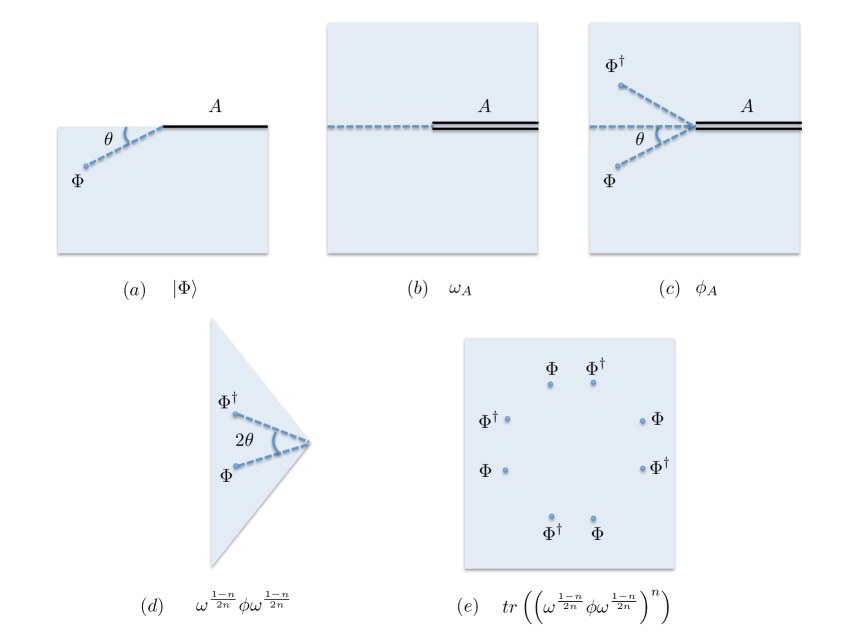
Figure 1: The Euclidean path integrals that prepare (a) excited state $|\Phi\rangle$, (b) vacuum density matrix on region $A$, (c) the density matrix of $A$ in the excited state. (d) The operator $\omega^{\frac{1-n}{2n}}\phi\omega^{\frac{1-n}{2n}}$ corresponds to a path-integral on a wedge of angular size $2\pi/n$. (e) The correlator that appears in the definition of the sandwiched Rényi divergence.

We would like to understand how the correlator in (75) changes as we change the region $A$. As we discussed in section 2, for a one-parameter family of smooth deformations given by $U_{\lambda}$ with $U_{0}=1$ that are symmetries of the vacuum state, the relative modular operator transforms according to

$$\Delta_{\Psi|\Omega}^{A(\lambda)}=U_{\lambda}^{\dagger}\Delta^{A}_{U_{\lambda}\Psi|\Omega}U_{\lambda}\ .$$ (76)

Plugging this into the definition of the sandwiched Rényi divergence we find

$$S^{A(\lambda)}_{\alpha}(\Phi\|\Omega)=S_{\alpha}^{A}(U_{\lambda}\Phi\|\Omega)\ .$$ (77)

The unitary $U_{\lambda}$ acts geometrically on local operators: $\Phi(z)\to\Phi^{(\lambda)}(z_{\lambda})$. The sandwiched Rényi divergence of the deformed region $A(\lambda)$ is given by the expression in (75) with $\Phi(z)$ replaced with $\Phi^{(\lambda)}(z_{\lambda})$.

To be specific, we consider the Rindler space parameterized by $(z,x_{\perp})$ where $z=x+i\tau$ and $x_{\perp}$ are the perpendicular directions. We focus on two classes of shape deformations and assume that operator $\Phi$ is a scalar:

1. Translations: The unitary $U_{\lambda}(\zeta)=e^{i\lambda P_{\zeta}}$ with $P_{\zeta}=\zeta_{0}P^{0}+\zeta_{1}P^{1}$ corresponds to a translation in $\zeta$ direction.

2. Null deformations: The unitary $U_{\lambda}(f,x_{\perp})=e^{i\lambda Q_{f}}$ with $Q_{f}=\int duf(x_{\perp})T_{uu}(u,x_{\perp})$ a conserved charge associated with deformations on a null hypersurface parameterized by $u=t-r$ and $x_{\perp}$.

The second class includes the first one as a special case. However, it is harder to work with $Q_{f}$ because, as opposed to $P_{\zeta}$, it is not a topological charge. If the states we consider are created by the action of only one operator acting on the vacuum, then $U_{\lambda}(f,x_{\perp})$ acts as:

$$U_{\lambda}(f,x_{\perp})\Phi(z,x_{\perp})|\Omega\rangle=U_{\lambda}(\zeta)\Phi(z,x_{\perp})|\Omega\rangle,$$ (78)

where $\zeta=f(x_{\perp})\partial_{u}$ is a null translation. We will use this simplifying assumption and postpone the study of the consequences of monotonicity under null deformations for general states to future work.

Consider the Euclidean translation $(\tau,x_{1})\to(\tau+\lambda\zeta_{0},x_{1}+\lambda)$ then

$$\Phi(-\tau_{0},x_{1})\to e^{-\lambda(\zeta_{0}P^{0}+P^{1})}\Phi(-\tau_{0},x_{1})e^{\lambda(\zeta_{0}P^{0}+P^{1})}=\Phi(-\tau_{0}-\lambda\zeta_{0},x_{1}-\lambda),$$

$$\Phi^{\dagger}(\tau_{0},x_{1})\to e^{-\lambda(-\bar{\zeta}_{0}P^{0}+P^{1})}\Phi^{\dagger}(\tau_{0},x_{1})e^{\lambda(-\bar{\zeta}_{0}P^{0}+P^{1})}=\Phi^{\dagger}(\tau_{0}+\lambda\bar{\zeta}_{0},x_{1}-\lambda),$$ (79)

where we have taken $a_{0}$ to be complex so that we can analytically continue it to real time. If we take $a_{0}$ to be pure imaginary the pair $\Phi^{\dagger}\Phi$ move together and the denominator in (75) stay the same. The other pairs of operators $\Phi^{\dagger}\Phi$ in the numerator of (75) are the same as $\Phi^{\dagger}\Phi$ above but rotated by $2\pi k/n$. To simplify our notation, we refer to $\Phi(z_{k})$ as $\Phi_{k}$.

Changing the region corresponds to moving $\Phi$ in the path-integral. The first derivatives in shape deformation corresponds to the first $\lambda$ derivatives in (6). The $m^{th}$ $\lambda$ derivative is a nested commutator of the pair $\Phi^{\dagger}\Phi$ with the momentum that generates the translation:

$$\frac{d^{m}}{d\lambda^{m}}(\Phi^{\dagger}\Phi)=\frac{1}{m!}[P_{\zeta},[P_{\zeta},\cdots,[P_{\zeta},\Phi^{\dagger}\Phi]]]\ .$$ (80)

The momentum $P_{\zeta}$ is a topological charge, so it can be written as

$$P_{\zeta}=\int_{C}d\Sigma^{i}\zeta^{j}T_{ij},$$ (81)

where $C$ is any codimension one surface that encircles the pair $\Phi^{\dagger}\Phi$ and no other operators. We choose this surface to be $x_{1}=c$ with $\tau_{0}\sin(\pi/n)<c<x_{1}$; see figure 2. The momentum $P_{\zeta}$ written on this surface is

$$P_{\zeta}=\int d\tau\left(T_{x_{1}x_{1}}+\zeta_{0}T_{\tau x_{1}}\right)=P^{1}+\zeta_{0}P^{0},$$ (82)

where $P^{0}$ and $P^{1}$ are momenta in $\tau$ and $x_{1}$ directions, respectively. We are interested in deformations of region $A$ that send $(x_{0},x_{1})\to(x_{0}+it,x_{1}+\lambda)$ with $t<1$, so we set $\zeta_{0}=it$. This makes sure $A(\lambda)\subset A(\lambda^{\prime})$ for any $\lambda<\lambda^{\prime}$.

To the first order in $\lambda$ by rotation symmetry we have

$$\partial_{\lambda}S^{A(\lambda)}_{1-\frac{1}{n}}(\Phi\|\Omega)_{\lambda=0}=\frac{n\langle[P_{\zeta},\Phi^{\dagger}_{0}\Phi_{0}]\Phi^{\dagger}_{1}\Phi_{1}\cdots\Phi^{\dagger}_{n-1}\Phi_{n-1}\rangle}{\langle\Phi^{\dagger}_{0}\Phi_{0}\cdots\Phi^{\dagger}_{n-1}\Phi_{n-1}\rangle}$$ (83)

where the factor of $n$ comes the rotation invariance of correlators. It is convenient to interpret the correlator above by choosing $\partial_{x_{1}}$ as the generator of time-translations. In this quantization frame, $P^{1}$ becomes the Hamiltonian and $P_{L}=iP^{0}$ becomes the Lorentzian momentum along a spacelike direction; see figure 2. Therefore, the monotonicity of Rényi divergences can be understood as the non-negativity of the following off-diagonal matrix elements of $H-tP_{L}$ with $0<t<1$:

$$\forall n\geq 1:\qquad\langle\Phi_{0}^{\dagger}\Phi_{0}|H-tP_{L}|\Phi_{1}^{\dagger}\Phi_{1}\cdots\Phi_{n-1}^{\dagger}\Phi_{n-1}\rangle\geq 0\ .$$ (84)

Note that the denominator in (83) is manifestly positive from reflection positivity around $\tau=0$. Since $H-tP_{L}=tP_{u}+(1-t)H$ with $P_{u}$ the null momentum in $u$ direction, we only need to consider the constraint at $t=0$ and $t=1$. When $n=2$ the inequality above follows from the positivity of $P_{u}$. To our knowledge, for $n>2$ this is a new constraint that does not follow from any of known inequalities in a trivial way. The physical interpretation of this result is that not only $H$ and $P_{u}$ are positive operators but also they have the following non-zero off-diagonal matrix elements:

$$\langle{\mathcal{O}}|P_{u}|{\mathcal{O}}_{n-1}\rangle\geq 0,\qquad\langle{\mathcal{O}}|H|{\mathcal{O}}_{n-1}\rangle\geq 0$$ (85)

where $|{\mathcal{O}}\rangle=|\Phi_{0}^{\dagger}\Phi_{0}\rangle$ and $|{\mathcal{O}}_{n-1}\rangle=|\Phi^{\dagger}_{1}\Phi_{1}\cdots\Phi^{\dagger}_{n-1}\Phi_{n-1}\rangle$.

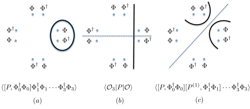
Figure 2: (a) The first derivative in shape deformation of the sandwiched Rényi divergence for $n=4$. The commutator is represented with the charge written as an integral on the codimension one surface encircling the pair $\Phi_{0}^{\dagger}\Phi_{0}$. (b) Same commutator with the charges written on a different surface, (c) A term that appears at the second order in deformation which is reflection symmetric around $\theta=\pi/2$. Note that $P^{(1)}$ is the same as $P$ but rotated by $\pi/2$.

Consider the quantization frame that chooses $\tau$ as the Euclidean time. Now the $2n$-point function without momentum commutators can be thought of as the the norm of a state $|\chi\rangle$ where $|\chi\rangle=|\Phi_{0}\Phi_{1}^{\dagger}\Phi_{1}\cdots\Phi^{\dagger}_{n/2}\rangle$ if $n$ is even and $|\chi\rangle=|\Phi_{0}\cdots\Phi_{(n-1)/2}^{\dagger}\Phi_{(n-1)/2}\rangle$ if $n$ is odd.

In the special case $\Phi=\Phi^{\dagger}$ the correlator is symmetric under the reflection $\tau\to-\tau$. Since this reflection sends $P^{0}$ to $-P^{0}$ but preserves $P^{1}$ we find that

$$\partial_{t}S_{1-\frac{1}{n}}(\Phi\|\Omega)|_{t=0}=0$$

$$\partial_{x}S_{1-\frac{1}{n}}(\Phi\|\Omega)|_{t=0}\geq 0\ .$$ (86)

Clearly, this holds only for the first derivative and just in the special case of a real field $\Phi=\Phi^{\dagger}$.

A conjecture

The sandwiched Rényi divergence is smooth at $\alpha=0$ and equal to the relative entropy. It was conjectured and recently argued that, in addition to the first derivative of relative entropy in deformation parameter that is positive due to monotonicity, the second null derivative of relative entropy is also non-negative in field theory [31, 32]. This is called the quantum null energy condition. In this subsection, we investigate the higher derivatives of the sandwiched Rényi divergence.

Let us start with $n=2$. From (80) we know that the $m^{th}$ derivatives in null deformations is the expectation value of the positive operator $P_{u}^{m}$ in the state $|{\mathcal{O}}\rangle$:

$$\partial_{\lambda}^{m}S_{1/2}(\Phi\|\Omega)=\frac{1}{m!}\langle{\mathcal{O}}|P_{u}^{m}|{\mathcal{O}}\rangle\geq 0\ .$$ (87)

Next, consider the second space-like derivative $(t=0)$ of Rényi divergences with $n>2$ for states that satisfy $\Phi=\Phi^{\dagger}$. Then,

$$\partial^{2}_{x}S^{A(\lambda)}_{1-\frac{1}{n}}(\Phi\|\Omega)_{\lambda=0} = \frac{n}{2}\frac{\langle[P^{1},[P^{1},\Phi_{0}\Phi_{0}]]\cdots\Phi_{n-1}\Phi_{n-1}\rangle}{\langle\Phi_{0}\Phi_{0}\cdots\Phi_{n-1}\Phi_{n-1}\rangle}$$

$$+\frac{n}{2}\sum_{k=2}^{n-1}\frac{\langle[P^{1},\Phi_{0}\Phi_{0}]\cdots[P^{(1,k)},\Phi_{k-1}\Phi_{k-1}]\cdots\Phi_{n-1}\Phi_{n-1}\rangle}{\langle\Phi_{0}\Phi_{0}\cdots\Phi_{n-1}\Phi_{n-1}\rangle}$$

where $P^{(1,k)}$ is the same operator as $P^{(1)}$ rotated by $2\pi k/n$; see figure 2. The first term above is symmetric under reflection around $\theta=0$, and the $k^{th}$ term in the sum is symmetric under the reflection around $\theta=\pi k/n$; see figure 2. Therefore, for the deformation generated by $\partial_{x_{1}}$ the second derivative of Rényi relative entropy is non-zero for all $n$ if $\Phi=\Phi^{\dagger}$:

$$\partial_{x}^{2}S(\Phi\|\Omega)\geq 0\ .$$ (88)

Repeating the argument above for a null deformation and the special state $\Phi=\Phi^{\dagger}$ we find that the second null derivative is also positive. Therefore, for this special class of states, we have proved our conjecture

$$\partial_{u}^{2}S(\Phi\|\Omega)\geq 0\ .$$ (89)

Examples

It is instructive to explicitly compute the sandwiched Rényi divergence and its derivatives in some simple theories. The theory has to be simple enough that we can compute the $2n$-point correlation functions. Two instances when we can access these correlators are free fields and small $\theta$ limit in conformal field theory.

Consider a two dimensional massless boson and a coherent operator $e^{i\beta\phi}$ with real $\beta$. Since this operator is a conformal primary, and there are the same number of operators in the numerator and the denominator of (75), the sandwiched Rényi divergence is independent of $r$ in $z_{k}^{(\pm)}=re^{i(\frac{2\pi k}{n}\pm\theta)}$. The $n$-point function of the coherent operator is given by [34]

$$\left\langle\prod_{k=0}^{n-1}e^{-i\beta_{k}\phi}(z_{k})\right\rangle=\prod_{k>i}(z_{k}-z_{i})^{\beta_{i}\beta_{k}}\ .$$ (90)

For the initial configuration at $\lambda=0$ we have

$$\frac{\left\langle\prod_{k=0}^{n-1}e^{-i\beta\phi}(z^{+}_{k})e^{i\beta\phi}(z^{-}_{k})\right\rangle}{\left\langle e^{-i\beta\phi}(z^{+}_{0})e^{i\beta\phi}(z_{0}^{-})\right\rangle^{n}}=\prod_{m=1}^{n-m}\left(\frac{\sin^{2}\left(\frac{\pi m}{n}\right)}{\sin\left(\frac{\pi m}{n}+\theta\right)\sin\left(\frac{\pi m}{n}-\theta\right)}\right)^{(n-m)\beta^{2}}=\left(\frac{n\sin\theta}{\sin(n\theta)}\right)^{n\beta^{2}}$$

The sandwiched Rényi divergence is [16]

$$S_{n}^{A(0)}(e^{i\beta\phi}\|\Omega)=\frac{n\beta^{2}}{n-1}\log\left(\frac{n\sin\theta}{\sin(n\theta)}\right)\ .$$ (91)

Initially starting at $(\tau=r\sin\theta,x_{1}=r\sin\theta)$ and deforming the region, the operator $\Phi_{0}$ moves to $(-\tau_{0}(1+\lambda\zeta_{0}),x_{1}(1-\lambda))$ and $\Phi^{\dagger}$ goes to $(\tau_{0}(1+\lambda\bar{\zeta}_{0}),x_{1}(1-\lambda))$, where $\bar{\zeta}_{0}$ is the complex conjugate of $\zeta_{0}$. Choosing $\zeta_{0}=it$ we find that $\langle\Phi^{\dagger}_{k}\Phi_{k}\rangle$ remains unchanged. For displaced operators from the $n$-point function formula we have

$$\frac{\left\langle\prod_{k=0}^{n-1}e^{-i\beta\phi}(z^{+}_{k}(\lambda))e^{i\beta\phi}(z^{-}_{k}(\lambda))\right\rangle}{\left\langle e^{-i\beta\phi}(z^{+}_{0})e^{i\beta\phi}(z_{0}^{-})\right\rangle^{n}}=\prod_{m=1}^{n-1}\left(\frac{4c(\theta)c(-\theta)\sin^{4}\left(\frac{m\pi}{n}\right)}{X(\theta)X(-\theta)}\right)^{(n-m)\frac{\beta^{2}}{2}}$$

$$X(\theta)=1-\cos\left(\frac{2\pi m}{n}+2\theta\right)+2\lambda\left(\cos\left(\frac{2\pi m}{n}+\theta\right)-\cos(\theta)\right)$$

$$+\lambda^{2}(1-t^{2})\left(1-\cos\left(\frac{2\pi m}{n}\right)\right)$$

$$c(\theta)=1-2\lambda(\cos\theta+it\sin\theta)+\lambda^{2}(1-t^{2})\ .$$ (92)

First consider the case $n=2$. Then,

$$X(\theta)=1+\cos(2\theta)-4\lambda\cos\theta+2\lambda^{2}(1-t^{2})$$ (93)

and

$$S_{1/2}^{A(\lambda)}(e^{i\beta\phi}\|\Omega) = \frac{\beta^{2}}{2}\log\left(\frac{4\left(4\lambda^{2}t^{2}\sin^{2}(\theta)+\left(1-2\lambda\cos(\theta)+\lambda^{2}\left(1-t^{2}\right)\right)^{2}\right)}{\left(1+\cos(2\theta)-4\lambda\cos(\theta)-2\lambda^{2}\left(t^{2}-1\right)\right)^{2}}\right)\ .$$ (94)

At $t=0$ we have

$$S_{1/2}^{A(\lambda)}(e^{i\beta\phi}\|\Omega)=\beta^{2}\log\left(\frac{(1+\lambda^{2}-2\lambda\cos\theta)}{(\lambda-\cos\theta)^{2}}\right)$$ (95)

According to Bernstein’s theorem a function $f(\lambda)$ has $\partial_{\lambda}^{k}f(\lambda)\geq 0$ for all $k$ if and only if $f(-\lambda)$ is the Laplace transform of a probability distribution $\mu(s)$ [35]:

$$f(-\lambda)=\int_{0}^{\infty}ds\>e^{-s\lambda}\mu(s)\ .$$ (96)

In many physics applications, the probability distribution $\mu(s)$ corresponds to the density of states that is a probability measure, and $f(-\lambda)$ is the partition function whose odd (even) derivatives in inverse temperature are negative (positive). The second Rényi divergence has an inverse Laplace transform

$$S_{1/2}^{A(-\lambda)}(e^{i\beta\phi}\|\Omega)=\int_{0}^{\infty}ds\>e^{-\lambda s}\mu(s)$$

$$\mu(s)=2\beta^{2}\frac{e^{-s\cos\theta}(1-\cos(s\sin\theta))}{s}\geq 0$$

$$\int_{0}^{\infty}ds\>\mu(s)=2\beta^{2}\log\sec\theta<\infty$$ (97)

which is indeed a probability measure. Therefore, we learn that all spatial derivatives of the second Rényi divergence are non-negative. Next, we consider $t=1$ that corresponds to a null deformation:

$$S_{1/2}(e^{i\beta\phi}\|\Omega)=\frac{\beta^{2}}{2}\log\left(\frac{1+4\lambda^{2}-4\lambda\cos\theta}{(2\lambda-\cos\theta)^{2}}\right)+\beta^{2}\log\sec\theta$$ (98)

The $\lambda$ dependent piece in (98) is the same as (95) with $\lambda\to 2\lambda$, hence all of its $\lambda$ derivatives as was proved before.

Same logic generalizes to $n>2$. Writing sandwiched Rényi for $n>2$ and $t=0$ as a Laplace transform we find

$$S_{1-\frac{1}{n}}^{A(-\lambda)}(e^{i\beta\phi}\|\Omega)=\frac{2\beta^{2}}{n-1}\sum_{m=1}^{n-1}(n-m)\int_{0}^{\infty}dse^{-\lambda s}\mu(s)$$

$$\mu(s)=\frac{e^{-s\cos\theta}}{s}\>\left(\cosh\left(s\sin\theta\cot\left(\frac{m\pi}{n}\right)\right)-\cos(s\sin\theta)\right)\geq 0$$ (99)

where both the numerator and the denominator are manifestly positive for $0\leq\theta\leq\pi/n$ and integer $n$. In the null case, it is easier to consider

$$S^{A(\lambda)}_{1-\frac{1}{n}}(e^{i\beta\phi}\|\Omega)-\frac{1}{2}S^{A(0)}_{1-\frac{1}{n}}(e^{i\beta\phi}\|\Omega)=\frac{\beta^{2}}{(n-1)}\sum_{m=1}^{n-1}(n-m)\int_{0}^{\infty}ds\>e^{-s\lambda}\mu(s)$$

$$\mu(s)=\frac{e^{-\frac{s}{2}\cos\theta}}{s}\>\left(\cosh\left(\frac{s}{2}\sin\theta\cot\left(\frac{m\pi}{n}\right)\right)-\cos\left(\frac{s}{2}\sin\theta\right)\right)\geq 0\ .$$ (100)

To summarize, we established that all spatial and null derivatives of Rényi divergences of coherent states with respect to vacuum are positive. The fact this holds for higher than two derivatives in deformations is special to coherent states. To show this, we consider the chiral primary operator $\partial\phi$ of the same theory.

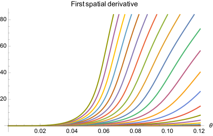
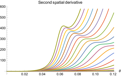
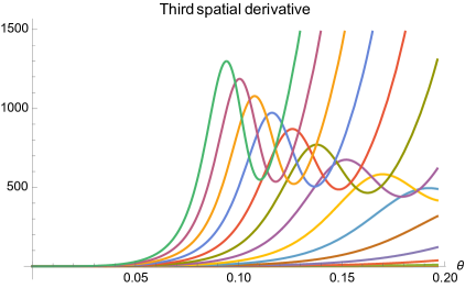
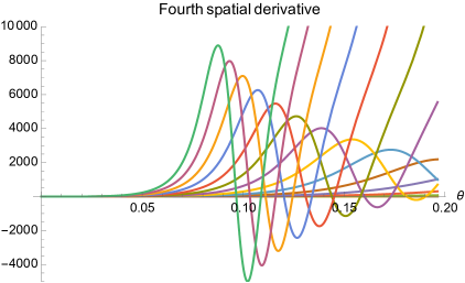
Figure 3: (top) The first and the second spatial derivatives of the sandwiched Rényi divergence for $n=2$ to $n=26$ are non-negative and consistent with monotonicity and our proof. (bottom) The third and the fourth spatial derivatives are plotted for $n=2$ to $n=16$. For large enough $n$, the fourth derivative becomes negative.

This operator has dimension $(1,0)$ and its $2n$-point functions were computed in [36]:

$$G_{n}=\left\langle\prod_{i=0}^{2n}(\partial\phi)^{\dagger}(\partial\phi)\right\rangle=\frac{1}{4^{n}}\det\left[\frac{1}{\sin\left(\frac{z_{i}-z_{j}}{2}\right)}\right]_{i,j\in[1,2n]}=\frac{\Gamma^{2}\left(\frac{1+n+n\csc(n\theta)}{2}\right)}{\Gamma^{2}\left(\frac{1-n+n\csc(n\theta)}{2}\right)}\ .$$ (101)

Therefore,

$$S_{1-\frac{1}{n}}(\partial\phi\|\Omega)=\frac{1}{n-1}\log\left((2\sin\theta)^{2n}G_{n}\right)$$ (102)

A spatial deformation correponds to $\cos\theta\to\cos\theta-\lambda$ in the formula above. Then, the first spatial derivative is given by

$$\partial_{\lambda}S^{A(\lambda)}_{1-\frac{1}{n}}(i\partial\phi\|\Omega)_{\lambda=0}$$

$$=\frac{2n\cos\theta}{(n-1)}\left(1-\frac{n\tan\theta}{\tan(n\theta)\sin(n\theta)}\left(\psi\left(\frac{1+n+n\csc(n\theta)}{2}\right)-\psi\left(\frac{1-n+n\csc(n\theta)}{2}\right)\right)\right)\ .$$

Note that this operator is real, so our proof of the non-negativity of the second derivative in spatial deformations applies to it. Figure 3 is a plot of the first four derivatives in spatial deformations. The first and the second derivatives of sandwiched Rényi divergence are non-negative as expected, however the fourth derivative becomes negative for large enough $n$.

As the second example, we consider the states of an interacting conformal field theory with $\theta\ll 1$. We expand each pair of operators in small $\theta$ using the operator product expansion:

$$\frac{\Phi_{k}^{\dagger}\Phi_{k}}{\langle\Phi_{k}^{\dagger}\Phi_{k}\rangle}=\sum_{p}(2\sin\theta)^{h_{p}}C^{p}_{\phi\phi}{\mathcal{O}}_{p}(z_{k}^{0},z_{k}^{1})$$

$$z_{k}^{0}=(\cos\theta-\lambda)\sin\left(\frac{2\pi m}{n}\right)-(\sin\theta+it\lambda)\cos\left(\frac{2\pi m}{n}\right)$$

$$z_{k}^{1}=(\cos\theta-\lambda)\cos\left(\frac{2\pi m}{n}\right)-(\sin\theta+it\lambda)\sin\left(\frac{2\pi m}{n}\right),$$ (103)

where ${\mathcal{O}}_{p}$ represent primaries and their descendants. The $2n$-point function in this limit is

$$\log\left(\frac{\left\langle\prod_{k=0}^{n-1}\Phi^{\dagger}(z^{+}_{k}(\lambda))\Phi(z^{-}_{k}(\lambda))\right\rangle}{\left\langle\prod_{k=0}^{n-1}\Phi^{\dagger}(z^{+}_{k})\Phi(z^{-}_{k})\right\rangle}\right)=\log\left(1+(C^{\Delta}_{\phi\phi})^{2}\sum_{m=1}^{n-1}\frac{(\theta)^{2\Delta}}{\left(c(\theta=0)\sin^{2}\left(\frac{m\pi}{n}\right)\right)^{\Delta}}+\cdots\right)$$

$$=\left(\frac{\theta}{1-2\lambda+\lambda^{2}(1-t^{2})}\right)^{\Delta}\>\sum_{m=1}^{n-1}\frac{1}{\sin^{2\Delta}\left(\frac{\pi m}{n}\right)}+\cdots$$ (104)

where $\Delta$ is the dimension of the lightest scalar primary. The inverse Laplace transform of the first term with $\lambda\to-\lambda$ is:

$$\left(\frac{\theta}{1+2\lambda+\lambda^{2}(1-t^{2})}\right)^{\Delta}=\int_{0}^{\infty}ds\>e^{-s\lambda}\>\mu_{t}(s)$$

$$\mu_{0}(s)=\frac{e^{-s}s^{2\Delta-1}}{\Gamma(2\Delta)}$$

$$\mu_{1}(s)=\frac{e^{-s/2}s^{\Delta-1}}{2^{\Delta}\Gamma(\Delta)},$$ (105)

which implies that all derivatives of the sandwiched Rényi divergence are non-negative for spatial and null deformations at this order in perturbation theory.

One can go to higher orders in perturbation theory. If we we focus on the case $t=0$ and assume that the second light primary has dimension $\Delta_{2}>\frac{3}{2}\Delta_{1}$, at the next order in perturbation theory we have

$$\log\left(1+(C^{\Delta}_{\phi\phi})^{2}\sum_{m=1}^{2}\frac{(2\sin\theta)^{2\Delta}}{\left(4c(\theta)\sin^{2}\left(\frac{m\pi}{3}\right)\right)^{\Delta}}+C^{\Delta}_{\Delta\Delta}\left(\frac{(2\sin\theta)}{3(1-\lambda)^{2}}\right)^{3\Delta}+\cdots\right)$$ (106)

Since the first order term is non-negative it is hard to use the monotonicity constraint to derive an inequality regarding only the OPE coefficients.

7 Discussion and Generalizations

In summary, we defined the sandwiched Rényi divergence as a Rényi generalization of relative entropy in any von Neumann algebra and explored the consequences of its monotonicity for correlation functions of field theory. We found new inequalities for correlation functions and conjectured a constraint on the second in null derivatives of the Rényi family that is a generalization of quantum null energy condition. It is interesting to explore the implications of these inequalities in large $N$ and holographic theories. The holographic dual of sandwiched Rényi divergences was constructed in [37]. It is natural to ask whether monotonicity can be used to constrain the effective field theory in the bulk. We postpone this to future work.

The physics interpretation of the Rényi divergences comes from their connection with the resource theory of thermodynamics. In an out-of-equilibrium quantum system with long-range interactions, there are many independent second laws of thermodynamics that constrain state transformations, each corresponding to a generalized free energy [38]. These free energies are precisely the sandwiched Rényi divergences and Petz divergences we studied here. This suggests that in conformal field theory and gravity the monotonicity of Rényi divergences for $n>1$ can be independent of the monotonicity of relative entropy. In fact, this was shown to be the case in holography in a recent work [27].

The averaged null energy condition is a universal constraint in all quantum field theories that was recently proved in [4] using the monotonicity of relative entropy. Later, the authors of [39] presented an alternative proof that relied on the analyticity and the causality of correlation functions. Our work sheds light on the connection between the two approaches by constructing information-theoretic quantities whose monotonicity is tied to the analyticity of correlation functions.

Finally, we would like to mention a few generalizations of this work. For most of our work here we focused only on the operator monotone function $f(z)=z^{\alpha}$. An arbitrary operator monotone function can be characterized in the following way: A function is operator monotone if and only if it has the representation [40]

$$f(z)=az+b+\int_{0}^{\infty}d\beta\mu(\beta)\left(\frac{1}{\beta}-\frac{1}{z+\beta}\right)$$ (107)

for $a,b\geq 0$ and $\mu(\beta)$ a measure that satisfies

$$\int_{0}^{1}\frac{d\beta}{\beta}\mu(\beta)+\int_{1}^{\infty}\frac{d\beta}{\beta^{2}}\mu(\beta)<\infty\ .$$ (108)

For instance, if we take $\mu(\beta)=\frac{\sin(\pi\alpha)}{\pi}\beta^{\alpha}$ the condition above is achieved if $0<\alpha<1$, and the function is simply $f(z)=z^{\alpha}$. The measures constructed from arbitrary operator monotone functions in finite quantum systems were studied in [25]. It would be interesting to see if one can relate the monotonicity of other $f(\Delta_{\Omega|\Psi})$ to correlation functions and obtain new constraints.

8 Acknowledgments

I am greatly indebted to Edward Witten whose suggestion to consider the non-commutative $L_{p}$ spaces initiated this work. I would also like to thank Nima Arkani-Hamed, Hong Liu, Raghu Mahajan, Srivatsan Rajagopal, Shu-Heng Shao, Douglas Stanford and Yoh Tanimoto for discussions at various stages of this project. This work was supported by a grant-in-aid (PHY-1606531) from the National Science Foundation.

Appendix A Proof of Properties Listed for Quasi-entropy

In this appendix we prove the the follwoing properties of the Petz quasi-entropy:

1. If $A\subset B$ and $a\in\mathcal{A}_{A}$ then it increases monotonically with system size:

   $$D^{A}_{\alpha,a}(\Phi\|\Omega)\leq D^{B}_{\alpha,a}(\Phi\|\Omega).$$

2. If $U$ is a unitary in $\mathcal{A}_{A}$ then $D_{\alpha,a}^{A}(U\Phi\|V\Omega)=D_{\alpha,V^{\dagger}aU}^{A}(\Phi\|\Omega)$.

3. It increases monotonically in $\alpha$. If $\alpha\leq\beta$ then $D^{A}_{\alpha,a}(\Phi\|\Omega)\leq D^{A}_{\beta,a}(\Phi\|\Omega)$.

Statements (1) and (2) follows respectively from the monotonicity relation in (16) and the transformation rule (11) for the relative modular operator under unitaries in the algebra. To show the monotonicity in $\alpha$ we consider the spectral decomposition of the relative modular operator:

$$\Delta^{-1}_{\Omega|\Phi}=\int_{0}^{\infty}\lambda\>P(d\lambda),$$ (109)

where $P(d\lambda)$ is a projection-valued measure. According to Holder’s inequality, if $\mu(\lambda)$ is a normalized probability measure, $\alpha>0$, $p>1$ and satisfies $\frac{1}{p}+\frac{1}{q}=1$ we have:

$$\int\lambda^{\alpha}d\mu(\lambda)\leq\left(\int\lambda^{p\alpha}d\mu(\lambda)\right)^{1/p}\left(\int d\mu(\lambda)\right)^{1/q}=\left(\int\lambda^{p\alpha}d\mu(\lambda)\right)^{1/p}\ .$$ (110)

Choosing $p=\beta/\alpha>1$ we obtain

$$\langle\Psi|\Delta_{\Omega|\Phi}^{-\alpha}|\Psi\rangle = \int\lambda^{\alpha}\langle\Psi|P(d\lambda)|\Psi\rangle\leq\left(\int\lambda^{\beta}\langle\Psi|P(d\lambda)|\Psi\rangle\right)^{\alpha/\beta}=\langle\Psi|\Delta_{\Omega|\Phi}^{-\beta}|\Psi\rangle^{\alpha/\beta},$$

where $|\Psi\rangle$ is an arbitrary state. This establishes monotonicity in $\alpha$. That is for $0\leq\alpha\leq\beta\leq 1$:

$$D_{\alpha,a}(\Phi\|\Omega)=\frac{1}{\alpha}\log\langle\Phi|a^{\dagger}\Delta_{\Omega|\Phi}^{-\alpha}a|\Phi\rangle\leq\frac{1}{\beta}\langle\Phi|a^{\dagger}\Delta_{\Omega|\Phi}^{-\beta}a|\Phi\rangle=D_{\beta,a}(\Phi\|\Omega)\ .$$ (111)

A similar argument using the spectral decomposition of $\Delta_{\Omega|\Phi}$ shows that the above equation holds for any $-1\leq\alpha\leq\beta\leq 1$.

Appendix B Proof of Properties Listed for Petz divergence

In this appendix, we prove of the properties of the Petz divergence listed below (19).

1. It is non-negative and vanishes when $A$ shrinks to zero.

2. It is invariant under the rotation of both vectors by the same unitary in $A$.

3. At $\alpha=0$ it is smooth and equal to the relative entropy.

4. Under swapping vectors $|\Phi\rangle$ and $|\Omega\rangle$ it satisfies

   $$D_{-\alpha}(\Phi\|\Omega)=\frac{1-\alpha}{\alpha}\>D_{\alpha-1}(\Omega\|\Phi)\ .$$ (112)

Statement (1) follows from the inequality in (15). Since Petz divergence is monotonic under the restriction to subregions and it vanishes as the region size shrinks to zero, it follows that it is non-negative. The second statement follows trivially by setting $a=1$ and $U=V$ in property (2) of quasi-entropies. The limit $\alpha\to 0$ from below and above equal the definition of relative from (9):

$$\lim_{\alpha\to 0}D_{\alpha}(\Phi\|\Omega)=-\log\langle\Phi|\log\Delta_{\Omega|\Phi}|\Phi\rangle=S(\Phi\|\Omega)\ .$$ (113)

Statement (4) says that under swapping vectors $|\Phi\rangle$ and $|\Omega\rangle$ the Petz divergence satisfies

$$D_{-\alpha}(\Phi\|\Omega)=\frac{1-\alpha}{\alpha}\>D_{\alpha-1}(\Omega\|\Phi)\ .$$ (114)

Remember that the Petz divergence is invariant under $|\Phi\rangle\to U^{\prime}|\Phi\rangle$ with $U^{\prime}$ a unitary in the $A^{\prime}$. This freedom can be used intelligently to satisfy $|\Phi\rangle=\Delta^{1/2}_{\Phi|\Omega}|\Omega\rangle$. Such a choice is called the vector representative of the state in the “natural cone”. See [7] for more detail. Equipped with this fact, the claim follows:

$$D_{-\alpha}(\Phi\|\Omega) = \frac{-1}{\alpha}\log\langle\Phi|\Delta_{\Omega|\Phi}^{\alpha}|\Phi\rangle$$ (115)

$$= \frac{1-\alpha}{\alpha}\left(\frac{1}{\alpha-1}\log\langle\Omega|\Delta^{1/2}_{\Phi|\Omega}\Delta_{\Omega|\Phi}^{\alpha}\Delta^{1/2}_{\Phi|\Omega}|\Omega\rangle\right)$$

$$= \frac{1-\alpha}{\alpha}\left(\frac{1}{\alpha-1}\log\langle\Omega|\Delta^{1-\alpha}_{\Phi|\Omega}|\Omega\rangle\right)$$

$$= \frac{1-\alpha}{\alpha}D_{\alpha-1}(\Omega\|\Phi)\ .$$

At the symmetric point $D_{-1/2}(\Phi\|\Omega)=D_{-1/2}(\Omega\|\Phi)=-2\log\langle\Phi|\Omega\rangle$. The non-negativity of the Petz divergence implies that $0\leq\langle\Phi|\Omega\rangle\leq 1$ for all normalized vectors in the natural cone.

Appendix C Proof of Inequality (32)

The claimed inequality in (32) is:

$$D_{\frac{\alpha}{1-\alpha}}(\Phi\|\Omega)\geq S_{\alpha}(\Phi\|\Omega)\geq D_{\alpha}(\Phi\|\Omega)\ .$$ (116)

The lower bound follows from the definition of the sandwiched Rényi divergences. The upper bound can be written as

$$\langle\Phi|\Delta_{\Omega|\Phi}^{-\frac{\alpha}{1-\alpha}}|\Omega\rangle^{\frac{(1-\alpha)}{\alpha}}\geq\sup_{\Psi}\langle\Phi|\Delta_{\Omega|\Psi}^{-\alpha}|\Phi\rangle^{\frac{1}{\alpha}}\ .$$ (117)

Using $|\Phi\rangle=\Delta_{\Omega|\Phi}^{-1/2}|\Omega\rangle$ it simplifies to

$$\|\Delta_{\Omega|\Phi}^{-\frac{1}{2(1-\alpha)}}|\Phi\rangle\|^{(1-\alpha)}\geq\sup_{\Psi}\|\Delta_{\Omega|\Psi}^{-\frac{\alpha}{2}}|\Phi\rangle\|\ .$$ (118)

Then, we use $(\Delta_{\Omega|\Psi}^{A})^{-1}=\Delta_{\Phi|\Omega}^{A^{\prime}}$ and $\alpha=1-\frac{2}{p}$ to we write it as

$$\|(\Delta^{A^{\prime}}_{\Phi|\Omega})^{\frac{p}{4}}|\Omega\rangle\|^{\frac{2}{p}}\geq\sup_{\Psi}\|(\Delta^{A^{\prime}}_{\Psi|\Omega})^{\frac{1}{2}-\frac{2}{p}}|\Phi\rangle\|\ .$$ (119)

This inequality is a generalization of the Araki-Lieb-Thirring inequality [41] to von Neumann algebras that can be proved using the interpolation theory of non-commutative $L_{p}$ spaces. However, this goes beyond the scope of this work and we refer the interested reader to the proof presented in Theorem 12 of [13].

References

- [1] H. Casini and M. Huerta, A finite entanglement entropy and the c-theorem, Physics Letters B 600 (2004), no. 1-2 142–150.
- [2] H. Casini and M. Huerta, Renormalization group running of the entanglement entropy of a circle, Physical Review D 85 (2012), no. 12 125016.
- [3] H. Casini, E. Testé, and G. Torroba, Markov property of the conformal field theory vacuum and the a theorem, Physical review letters 118 (2017), no. 26 261602.
- [4] T. Faulkner, R. G. Leigh, O. Parrikar, and H. Wang, Modular hamiltonians for deformed half-spaces and the averaged null energy condition, Journal of High Energy Physics 2016 (2016), no. 9 38.
- [5] A. C. Wall, Proof of the generalized second law for rapidly changing fields and arbitrary horizon slices, Physical Review D 85 (2012), no. 10 104049.
- [6] E. Witten, Notes on Some Entanglement Properties of Quantum Field Theory, arXiv:1803.04993.
- [7] R. Haag, Local quantum physics: Fields, particles, algebras. 1992.
- [8] H. Araki, Relative entropy of states of von neumann algebras, Publications of the Research Institute for Mathematical Sciences 11 (1976), no. 3 809–833.
- [9] V. Vedral, The role of relative entropy in quantum information theory, Reviews of Modern Physics 74 (2002), no. 1 197.
- [10] H. Araki and T. Masuda, Positive cones and lp-spaces for von neumann algebras, Publications of the Research Institute for Mathematical Sciences 18 (1982), no. 2 759–831.
- [11] V. Jaksic, Y. Ogata, Y. Pautrat, and C.-A. Pillet, Entropic fluctuations in quantum statistical mechanics. an introduction, arXiv preprint arXiv:1106.3786 (2011).
- [12] A. Jencová, Rényi relative entropies and noncommutative -spaces, arXiv preprint arXiv:1609.08462 (2016).
- [13] M. Berta, V. B. Scholz, and M. Tomamichel, Rényi divergences as weighted non-commutative vector-valued -spaces, in Annales Henri Poincaré, arXiv:1608.05317, vol. 19, pp. 1843–1867, Springer, 2018.
- [14] R. L. Frank and E. H. Lieb, Monotonicity of a relative rényi entropy, Journal of Mathematical Physics 54 (2013), no. 12 122201.
- [15] S. Beigi, Sandwiched rényi divergence satisfies data processing inequality, Journal of Mathematical Physics 54 (2013), no. 12 122202.
- [16] N. Lashkari, Relative entropies in conformal field theory, Physical review letters 113 (2014), no. 5 051602.
- [17] V. F. R. Jones., Von Neumann Algebras. 1992.
- [18] H.-J. Borchers, On revolutionizing quantum field theory with tomita’s modular theory, Journal of mathematical Physics 41 (2000), no. 6 3604–3673.
- [19] M. A. Nielsen and D. Petz, A simple proof of the strong subadditivity inequality, arXiv preprint quant-ph/0408130 (2004).
- [20] D. Petz, Quasi-entropies for states of a von neumann algebra, Publications of the Research Institute for Mathematical Sciences 21 (1985), no. 4 787–800.
- [21] M. Müller-Lennert, F. Dupuis, O. Szehr, S. Fehr, and M. Tomamichel, On quantum rényi entropies: A new generalization and some properties, Journal of Mathematical Physics 54 (2013), no. 12 122203.
- [22] M. M. Wilde, A. Winter, and D. Yang, Strong converse for the classical capacity of entanglement-breaking and hadamard channels via a sandwiched rényi relative entropy, Communications in Mathematical Physics 331 (2014), no. 2 593–622.
- [23] R. Haag and J. A. Swieca, When does a quantum field theory describe particles?, Communications in Mathematical Physics 1 (1965), no. 4 308–320.
- [24] A. Uhlmann, The “transition probability” in the state space of aalgebra, Reports on Mathematical Physics 9 (1976), no. 2 273–279.
- [25] M. M. Wilde, Optimized quantum f-divergences and data processing, Journal of Physics A: Mathematical and Theoretical 51 (2018), no. 37 374002.
- [26] N. Lashkari, H. Liu, and S. Rajagopal, Modular Flow of Excited States, arXiv:1811.05052.
- [27] A. Bernamonti, F. Galli, R. C. Myers, and J. Oppenheim, Holographic second laws of black hole thermodynamics, arXiv preprint arXiv:1803.03633 (2018).
- [28] H. Casini, E. Testé, and G. Torroba, Modular hamiltonians on the null plane and the markov property of the vacuum state, Journal of Physics A: Mathematical and Theoretical 50 (2017), no. 36 364001.
- [29] N. Lashkari, Entanglement at a scale and renormalization monotones, arXiv preprint arXiv:1704.05077 (2017).
- [30] K. Osterwalder and R. Schrader, Axioms for euclidean green’s functions ii, Communications in Mathematical Physics 42 (1975), no. 3 281–305.
- [31] R. Bousso, Z. Fisher, S. Leichenauer, and A. C. Wall, Quantum focusing conjecture, Physical Review D 93 (2016), no. 6 064044.
- [32] S. Balakrishnan, T. Faulkner, Z. U. Khandker, and H. Wang, A general proof of the quantum null energy condition, arXiv preprint arXiv:1706.09432 (2017).
- [33] H. Casini, R. Medina, I. S. Landea, and G. Torroba, Rényi relative entropies and renormalization group flows, Journal of High Energy Physics 2018 (2018), no. 9 166.
- [34] P. Francesco, P. Mathieu, and D. Sénéchal, Conformal field theory. Springer Science & Business Media, 2012.
- [35] S. Bernstein, Sur les fonctions absolument monotones, Acta Mathematica 52 (1929), no. 1 1–66.
- [36] P. Calabrese, F. H. Essler, and A. M. Läuchli, Entanglement entropies of the quarter filled hubbard model, Journal of Statistical Mechanics: Theory and Experiment 2014 (2014), no. 9 P09025.
- [37] N. Lashkari, J. Lin, H. Ooguri, B. Stoica, and M. Van Raamsdonk, Gravitational positive energy theorems from information inequalities, Progress of Theoretical and Experimental Physics 2016 (2016), no. 12.
- [38] F. Brandao, M. Horodecki, N. Ng, J. Oppenheim, and S. Wehner, The second laws of quantum thermodynamics, Proceedings of the National Academy of Sciences 112 (2015), no. 11 3275–3279.
- [39] T. Hartman, S. Kundu, and A. Tajdini, Averaged null energy condition from causality, Journal of High Energy Physics 2017 (2017), no. 7 66.
- [40] R. L. Schilling, R. Song, and Z. Vondracek, Bernstein functions: theory and applications, vol. 37. Walter de Gruyter, 2012.
- [41] E. H. Lieb and W. E. Thirring, Inequalities for the moments of the eigenvalues of the schrodinger hamiltonian and their relation to sobolev inequalities, in The Stability of Matter: From Atoms to Stars, pp. 135–169. Springer, 1991.