Axisymmetric lattice Boltzmann model for multiphase flows with large density ratio

Abstract

In this paper, a novel lattice Boltzmann (LB) model based on the Allen-Cahn phase-field theory is proposed for simulating axisymmetric multiphase flows. The most striking feature of the model is that it enables to handle multiphase flows with large density ratio, which are unavailable in all previous axisymmetric LB models. The present model utilizes two LB evolution equations, one of which is used to solve fluid interface, and another is adopted to solve hydrodynamic properties. To simulate axisymmetric multiphase flows effectively, the appropriate source term and equilibrium distribution function are introduced into the LB equation for interface tracking, and simultaneously, a simple and efficient forcing distribution function is also delicately designed in the LB equation for hydrodynamic properties. Unlike many existing LB models, the source and forcing terms of the model arising from the axisymmetric effect include no additional gradients, and consequently, the present model contains only one non-local phase field variable, which in this regard is much simpler. In addition, to enhance the model’s numerical stability, an advanced multiple-relaxation-time (MRT) model is also applied for the collision operator. We further conducted the Chapman-Enskog analysis to demonstrate the consistencies of our present MRT-LB model with the axisymmetric Allen-Cahn equation and hydrodynamic equations. A series of numerical examples, including static droplet, oscillation of a viscous droplet, breakup of a liquid thread, and bubble rising in a continuous phase, are used to test the performance of the proposed model. It is found that the present model can generate relatively small spurious velocities and can capture interfacial dynamics with higher accuracy than the previously improved axisymmetric LB model. Besides, it is also found that our present numerical results show excellent agreement with analytical solutions or available experimental data for a wide range of density ratios, which highlights the strengths of the proposed model.

1 Introduction

Multiphase fluid flows are ubiquitous in nature and are of considerable interest in both scientific and engineering fields. In spite of improving experimental studies of these multiphase phenomena, numerical modeling becomes an increasingly important approach with the rapid development of computer technology and gradual enrichment of computing methods. And also, it can provide a convenient access to physical quantities, such as variational interface shapes, fluid velocity across interface, pressure distribution inside and outside bulk phase, which are usually difficult to measure experimentally. Nonetheless, it still remains an intractable task to the modeling of multiphase flows and further develop efficient numerical algorithms that can accurately describe physical phenomena behind such flows. The reasons behind the challenges lie in the complexity of interface dynamics among multispecies fluids, density and viscosity jumps across the interface, and surface tension force modeling. Several numerical methods to date have been proposed for simulating multiphase flows, which can be roughly divided into two categories: sharp-interface methods, and diffusion-interface methods. The former methods commonly include the volume-of-fluid method [1], front-tracking method [2] and level set method [3]. In this type of traditional methods, one might solve continuum mechanics equations coupled with a suitable technique to track the phase interface. The interface needs to be captured manually based on some complex ad-hoc criteria, and fluid properties in these methods such as density and viscosity vary sharply at the interface. Therefore, they in this regard are not suitable for handling multiphase flows with large interface topological change [4, 5]. As for the latter methods, one replaces the sharp interface with a transition region across which fluid physical properties are allowed to change smoothly. This feature makes them more potential for simulating complex interfacial dynamic problems. Among diffusion-interface approaches, the phase-field method [6] and lattice Boltzmann (LB) method [7, 8] are two popular ones. In the phase-field method, the thermodynamic behavior of a multiphase system is described by the free energy as a function of an order parameter, which is used to capture phase interface. The interfacial governing equation for the order parameter is formulated as the convective Cahn-Hilliard [9, 6] or Allen-Cahn (AC) [10, 11] equation, which is usually solved by using a finite difference like scheme in phase field modelling. Therefore the phase field method will inherit some certain weaknesses rooted in the conventional numerical methods.

Alternatively, the LB method [7, 8] has received great attention for modelling hydrodynamic phenomena and in particular for multiphase flows. It is a mesoscopic method based on the kinetic equation for the particle distribution function, connecting the bridge between the macroscopic continuum model and molecular dynamics. Due to its mesoscopic nature, the LB method has several distinct advantages over the traditional numerical methods, such as the simplicity of algorithmic, nature parallelization and easy implementation of complex boundary. Particularly, the intermolecular interactions in a multiphase system can be incorporated directly in the framework of LB method, while they are difficult to handle in traditional numerical methods. Historically, from different physical pictures of the interactions, several types of LB models have been established for simulating multiphase flows, which include the color-gradient model [12], pseudo-potential model [13], free energy model [14], and phase-field based model [15, 16, 17, 18]. Some advanced LB models based on these original models have also been proposed in succession and interesting readers can refer to good reviews [20, 19] of this field and the references therein.

In practice, there exists many multiphase fluid problems that display axial symmetry. Examples include head-on collision of binary droplets [21, 22], bubble rising in a continuous phase [23, 24], droplet formation in micro-channel [25, 26], droplet splashing on a solid surface or wetting liquid film [27, 28], and so on. The most natural manner to simulate such axisymmetric flows is to apply a three-dimensional (3D) LB multiphase model with suitable curved boundary conditions. This treatment, however, does not take any advantages of the axisymmetric property of flow. If we recognize the fact that 3D axisymmetric flows can reduce to the two-dimensional (2D) ones in meridian plane, an effective approach in this regard is to develop quasi-2D LB models for simulating these flows. Up to now, some scholars have made an effort to construct effective axisymmetric models based on the LB method, whereas most of them are proposed for single-phase flows within the isothermal and thermal systems [29, 30, 31, 32, 33, 34]. The first axisymmetric LB model for multiphase flows was attributed to Premnath and Abraham [35], who introduced some suitable source terms in the Cartesian coordinate multiphase model of He et al. [15]. The source terms are used to account for the axisymmetric contribution of inertial, viscous and surface tension forces, while they contains many complex gradients of density and velocity and thus undermine the simplicity of the model. In addition, the model has a drawback inherited in He’s model that the available highest density ratio is limited to 15. And also based on the multiphase model of He et al. [15], Huang et al. [24] presented an improved axisymmetric LB model, in which a mass correction step is imposed in every numerical iteration. They applied this model to the simulation of bubble rising, and found rather good agreement with experiments. However, the highest density ratio in the simulation is limited to 15.5, and the model would undergo numerical instability with the increasing density ratio, as they stated. To remove this limitation, Mukherjee and Abraham [36] proposed an axisymmetric counterpart based on the high-density-ratio model of Lee and Lin [16], in which some source terms relating to the density and velocity gradients are also included. To improve numerical stability, they also used a three-stage mixing discretization scheme, which unfortunately could induce the violation of the mass conservation [37]. Later, Huang et al. [38] put forward a hybrid LB model for axisymmetric binary flows, where a finite difference scheme is used to solve the convective Cahn-Hilliard equation for interface capturing and a multiple-relaxation-time (MRT) LB scheme is adopted for solving the Navier-Stokes (NS) equations. The densities of binary fluids are supposed to be uniform in the given NS equations, and therefore their model in theory can only be applicable for density-matched two-phase flows. The extension of the popular pseudo-potential model [13] to the axisymmetric version was conducted by Srivastava et al. [39]. Recently, Liang et al. [40] proposed a Cahn-Hilliard phase-field based LB model for axisymmetric multiphase flows. One distinct feature of this model is that the added source terms representing the axisymmetric effect contain no gradients, thus simplifying the computation. The model is also demonstrated to be accurate for simulating multiphase flows with moderate density ratios, while it is unable to tackle large-density-ratio cases. More recently, Liu et al. [41] developed a color-gradient LB model for axisymmetric multicomponent flows. This model can deal with binary fluids with high viscosity ratio, whereas the density ratio considered is very small.

As reviewed above, several types of LB models have been proposed for axisymmetric multiphase flows, and all these models are restricted to the flows with small or moderate density contrasts. Generally, the density ratio can approach 1000 for a realistic liquid-vapor system, and to develop a high-density-ratio multiphase model is very attractive in LB community. In this paper, we intend to present a simple, accurate and also robust LB model for axisymmetric multiphase flows, which can tolerate large density contrasts. The proposed LB model is based on the AC phase field theory, which involves a lower-order diffusion term compared with the Cahn-Hilliard equation, and thus is expected to achieve a better numerical accuracy. Modified equilibrium distribution functions and simplified forcing distribution functions are also incorporated in the model to recover the correct axisymmetric AC and NS equations. Besides, unlike most of available LB models [35, 24, 36, 38, 39], the introduced source terms arising from the axisymmetric effect contain no gradients in the present model. The rest of this paper is organized as follows. In Sec 2, the governing equations and their axisymmetric formulations are first given, and then a novel axisymmetric LB model based on the AC phase-field theory are proposed. Numerical validations for the present model can be found in Sec 3, and at last, we made a brief summary in Sec. 4.

2 GOVERNING EQUATIONS AND MATHEMATICAL MODEL

2.1 Governing equations

The AC equation contains only at most a second-order gradient diffusion term, which can be more efficient and less dispersive in solving the phase interface compared with the commonly used Cahn-Hilliard theory [42, 43, 44, 45]. Therefore the interface tracking equation in this study is built upon the AC phase field theory. The original AC equation was not globally conservative, and recently reformulated into the conservative form [11] based on the work of Sun and Beckermann [10]. This specific formulation is commonly referred as the conservative phase-field model and will be adopted here. Then the conservative AC equation for interface tracking can be written as [11, 42, 46],

$${{\partial\phi}\over{\partial t}}+\nabla\cdot(\phi\textbf{u})=\nabla\cdot{[M(\nabla{\phi}-\lambda\textbf{n})]},$$ (1)

where $\phi$ is the order parameter acting as a phase field to distinguish different fluids, u is the fluid velocity, $M$ is the mobility, n is the unit vector normal to the interface and is calculated as $\textbf{n}={{\nabla\phi}/{|\nabla\phi|}}$, $\lambda$ can be expressed by

$$\lambda=-{4(\phi-1)\phi\over{W}},$$ (2)

where $W$ is the interfacial thickness, the phase field $\phi$ takes 1 and 0 in the bulk regions of the liquid and vapor fluids, respectively, and $\phi=0.5$ indicates the phase interface of binary fluids. To simulate hydrodynamic flows, the AC equation should be coupled with the incompressible NS equations, which can be written as [2, 45]

$$\nabla\cdot{\bf{u}}=0,$$ (3a)

$${{\partial({\rho\bf{u}}})\over{\partial t}}+\nabla\cdot(\rho{\bf{u}}{\bf{u}})=-\nabla p+\nabla\cdot\left[{\nu\rho(\nabla{\bf{u}}+\nabla{{\bf{u}}^{T}})}\right]+{{\bf{F}}_{s}}+{\bf{G}},$$ (3b)

where $p$ is the hydrodynamic pressure, $\nu$ is the kinematic viscosity, G is the possible external force, $\textbf{F}_{s}$ is the surface tension force. According to Ref. [47], there exists several treatments in terms of surface tension force, which could give rise to different performances. To reduce the spurious velocity, in this work we choose the widely used the potential form $\textbf{F}_{s}=\mu\nabla\phi$ [17, 43, 40], where $\mu$ is the chemical potential given by

$$\mu=4\beta\phi(\phi-1)(\phi-0.5)-k\nabla^{2}\phi,$$ (4)

where the parameters $\beta$ and $k$ can be determined by the surface tension $\sigma$ and the interfacial thickness, i.e., $k=1.5\sigma W$, $\beta=12\sigma/W$.

We now performed the coordinate transformation to derive the governing equations of isothermal multiphase flow in the axisymmetric system. The transformation is given by

$(x,y,z)\rightarrow(r,\theta,z)$

with the relations $x=r\cos\theta$, $y=r\sin\theta$, where $r$, $z$, $\theta$ denote the radial, axial and azimuthal directions, respectively. The flows are assumed to have no swirl here and thus we can set the azimuthal velocity and azimuthal coordinate derivatives to be zero. In this case, the resulting macroscopic equations in the axisymmetric framework can be expressed by

$$\partial_{t}\phi+\partial_{\alpha}(\phi u_{\alpha})+\frac{\phi{u_{r}}}{r}=\partial_{\alpha}(M\partial_{\alpha}\phi)+\frac{M\partial_{r}\phi}{r}-M\partial_{\alpha}(\lambda{n_{\alpha}})-\frac{M\lambda{\partial_{r}}\phi}{r|\nabla\phi|}$$ (5)

and

$$\partial_{\alpha}u_{\alpha}+\frac{u_{r}}{r}=0,$$ (6a)

$$\partial_{t}(\rho{u_{\beta}})+{\partial_{\alpha}}(\rho{u_{\alpha}}u_{\beta})=-\partial_{\beta}{p}+{\partial_{\alpha}}\nu\rho({\partial_{\alpha}}u_{\beta}+{\partial_{\beta}}u_{\alpha})+{\tilde{F}_{s\beta}}+G_{\beta}+\frac{\nu\rho(\partial_{r}{u_{\beta}}+\partial_{\beta}{u_{r}})}{r}-\frac{2\rho\nu{u_{r}}\delta_{{\beta}r}}{r^{2}}-{{\rho u_{r}u_{\alpha}}\over{r}},$$ (6b)

where $\alpha,\beta=\{r,z\}$, $\delta$ is the Kronecker function, ${\tilde{F}_{s\beta}}$ is the modified surface tension force given by ${\tilde{F}_{s\beta}}=\tilde{\mu}\nabla{\phi}$, and $\tilde{\mu}=\mu-k\partial_{r}{\phi}/r$. From Eqs. (5) and (6), it can be clearly found that some additional source terms are generated due to the axisymmetric effect. These source terms contain some gradients on the fluid velocity, and seem to be implemented complicatedly. To our knowledge, most of previously proposed axisymmetric LB models [29, 32, 34, 35, 24, 36, 38, 39] for hydrodynamic flows were constructed based on the governing equation (6), which thus makes them more complex than the standard models in the Cartesian coordinate system. Alternatively, we convert the governing equations (5) and (6) in another form. With some algebraic manipulations, the derived macroscopic equations can be presented as

$$\partial_{t}(r\phi)+\partial_{\alpha}(r\phi u_{\alpha}+M\phi\delta_{\alpha r})=\partial_{\alpha}[M\partial_{\alpha}(r\phi)-Mr\lambda n_{\alpha}]$$ (7)

and

$$\partial_{\alpha}(ru_{\alpha})=0,$$ (8a)

$$\partial_{t}(r\rho{u_{\beta}})+{\partial_{\alpha}}(r\rho{u_{\alpha}}u_{\beta})=-\partial_{\beta}(rp)+{\partial_{\alpha}}[r\nu\rho({\partial_{\alpha}}u_{\beta}+{\partial_{\beta}}u_{\alpha})]+r(\tilde{F}_{s\beta}+G_{\beta})+(p-{2\rho\nu\over r}u_{r})\delta_{\beta r}.$$ (8b)

The present LB model will be built upon the macroscopic equations (7) and (8), which utilizes two LB evolution equations, one of them is used to solve the axisymmetric AC equation, and another for solving the axisymmetric NS equations. It will be demonstrated below that the introduced source terms representing the axisymmetric contributions contain no gradients in the present model.

2.2 Axisymmetric LB model for the Allen-Cahn equation

Based on the collision operators, the LB approach can be roughly divided into four categories, including the MRT model [48], the two-relaxation-time model [49], the single-relaxation-time model [50], and the entropic LB model [51]. To date, these models all have their own impressive versatility in simulating hydrodynamic flows, while the MRT model in comparison has its superiority in terms of stability and accuracy, and thus will be used in the present LB modelling for multiphase flows. The LB evolution equation of the MRT model for the axisymmetric AC equation can be proposed as

$$f_{i}(\textbf{x}+\textbf{c}_{i}\delta_{t},t+\delta_{t})-f_{i}(\textbf{x},t)=\Omega_{i}(\textbf{x},t)+\delta_{t}{F}_{i}(\textbf{x},t),$$ (9)

where the collision operator $\Omega_{i}$ is defined by

$$\Omega_{i}(\textbf{x},t)=-({{{\bf{M}}^{-1}}{{\bf{S}}^{f}}{\bf{M}})_{ij}}[f_{j}(\textbf{x},t)-f_{j}^{eq}(\textbf{x},t)],$$ (10)

where $f_{i}(\textbf{x},t)$ is the phase-field distribution function associated with the discrete velocity $\textbf{c}_{i}$ at position x and time $t$, $f_{i}^{eq}(\textbf{x},t)$ is the equilibrium distribution function. To match the target equation, we design a new equilibrium distribution function as

$$f_{i}^{eq}=\omega_{i}\left[r\phi+{c_{i\alpha}(r\phi u_{\alpha}+M\phi\delta_{\alpha r})\over{c_{s}^{2}}}\right],$$ (11)

where $c_{s}$ is lattice sound speed, $\omega_{i}$ are the weighting coefficients. $\omega_{i}$ and $\textbf{c}_{i}$ depend on the choice of the discrete-velocity lattice model. For plane flows, the popular D2Q9 lattice model [50, 17, 18, 52] is adopted here, and $\omega_{i}$ can be then given by $\omega_{0}=4/9$, $\omega_{1-4}=1/9$, $\omega_{5-8}=1/36$, and $\textbf{c}_{i}$ is defined as

$$\mathbf{c}_{i}=\left\{\begin{array}[]{ll}(0,0)c,&\textrm{ $i=0$},\\ (\cos[(i-1)\pi/2],\sin[(i-1)\pi/2])c,&\textrm{ $i=1-4$},\\ \sqrt{2}(\cos[(i-5)\pi/2+\pi/4],\sin[(i-5)\pi/2+\pi/4])c,&\textrm{ $i=5-8$},\end{array}\right.$$ (12)

where $c=\delta_{x}/\delta_{t}$ denotes the lattice speed with $\delta_{x}$ and $\delta_{t}$ representing the lattice spacing and the time step, respectively, and $c_{s}=c/\sqrt{3}$. By convention, $\delta_{x}$ and $\delta_{t}$ in the study of multiphase flows are set to be length and time units, i.e., $\delta_{x}=\delta_{t}=1$. In Eq. (10), M is the transformation matrix, which is used to project the distribution function in the discrete-velocity space onto the ones in the moment space. Based on the D2Q9 lattice structure, it can be given by [48]

$$\bf{M}=\left(\begin{array}[]{rrrrrrrrr}1&1&1&1&1&1&1&1&1\\ -4&-1&-1&-1&-1&2&2&2&2\\ 4&-2&-2&-2&-2&1&1&1&1\\ 0&1&0&-1&0&1&-1&-1&1\\ 0&-2&0&2&0&1&-1&-1&1\\ 0&0&1&0&-1&1&1&-1&-1\\ 0&0&-2&0&2&1&1&-1&-1\\ 0&1&-1&1&-1&0&0&0&0\\ 0&0&0&0&0&1&-1&1&-1\end{array}\right),$$

and ${\bf{S}}^{f}$ in Eq. (10) is a diagonal relaxation matrix,

$${\bf{S}}^{f}=diag(s_{0}^{f},s_{1}^{f},s_{2}^{f},s_{3}^{f},s_{4}^{f},s_{5}^{f},s_{6}^{f},s_{7}^{f},s_{8}^{f}),$$ (13)

where $0\leq s_{i}^{f}<2$. To simplify the LB algorithm, one part of the diffusion term in Eq. (7) is treat as the source term here, and then a novel discrete source term is introduced as

$${F}_{i}=[\textbf{M}^{-1}(\textbf{I}-{\textbf{S}^{f}\over 2})\textbf{M}]_{ij}{R_{j}},$$ (14)

where I is the unit matrix, and $R_{i}$ is defined by

$$R_{i}={\omega_{i}c_{i\alpha}[\partial_{t}(r\phi u_{\alpha}+M\phi\delta_{\alpha r})+c_{s}^{2}rn_{\alpha}\lambda]\over{c_{s}^{2}}}.$$ (15)

In the present model, the phase field variable $\phi$ is derived by the summation of the distribution function $f_{i}$, and then is computed by

$$\phi=\frac{1}{r}\sum\limits_{i}{{f_{i}}}.$$ (16)

Physically, the density distribution in a multiphase system is consistent with that of the phase field variable. To satisfy this property, we take the linear interpolation scheme to determine the fluid density,

$$\rho=\phi\rho_{l}+(1-\phi)\rho_{g},$$ (17)

where $\rho_{l}$ and $\rho_{g}$ denote the liquid and gas fluid densities, respectively. We also carried out the Chapman-Enskog analysis to demonstrate the consistency of the present model with the target equation (7). Applying the multiscale expansions to Eq. (9), it is found in Appendix A that the axisymmetric AC equation can be recovered exactly from the present model, and the mobility is given by

$$M=c_{s}^{2}\delta_{t}(\tau_{f}-\frac{1}{2}),$$ (18)

where $1/\tau_{f}={s_{3}^{f}}={s_{5}^{f}}$. In comparison with the standard LB model [42] for AC equation, it is found that the introduced source terms to account for the axisymmetric effect include no additional gradient in the present model.

We now give a discussion on implementation of the MRT model. Generally, the MRT-LB equation (9) can be solved in two steps, including the collision process,

$$f_{i}^{+}=f_{i}(\textbf{x},t)-({{{\bf{M}}^{-1}}{{\bf{S}}^{f}}{\bf{M}})_{ij}}[f_{j}(\textbf{x},t)-f_{j}^{eq}(\textbf{x},t)]+\delta_{t}{F}_{i}(\textbf{x},t)$$ (19)

and the propagation process,

$$f_{i}(\textbf{x}+\textbf{c}_{i}\delta_{t},t+\delta_{t})=f_{i}^{+}.$$ (20)

To reduce the matrix operations, it is wise that the collision process of MRT model is conducted in the moment space. By premultiplying the matrix M, the equilibrium distribution function in moment space is derived as

$$\textbf{ Mf}^{eq}=\left(r\phi,-2r\phi,r\phi,\frac{r\phi{u_{z}}}{c},-\frac{r\phi{u_{z}}}{c},\frac{r\phi{u_{r}}+M\phi}{c},-\frac{r\phi{u_{r}}+M\phi}{c},0,0\right)^{T},$$ (21)

where $u_{r}$ and $u_{z}$ are the radial and axial components of velocity. Similarly, the discrete source term $R_{i}$ in the moment space can also be obtained as

$$\textbf{ MR}=(0,0,0,mR_{1},-mR_{1},mR_{2},-mR_{2},0,0)^{T},$$ (22)

where $mR_{1}$ and $mR_{2}$ are given by

$$mR_{1}=\frac{\partial_{t}({r\phi{u_{z}}})+c_{s}^{2}r{n_{z}}\lambda}{c},mR_{2}=\frac{\partial_{t}({r\phi{u_{r}}}+M\phi)+c_{s}^{2}r{n_{r}}\lambda}{c}.$$ (23)

At the end of this subsection, we also would like to stress that the present MRT model for the axisymmetric AC equation can reduce to the SRT counterpart when the relaxation factor $s_{i}^{f}$ in Eq. (13) equals to each other, and thus the SRT model is only one special case of the MRT model. In this case, the more freedom in the choice of the relaxation factors can provide more potential for the MRT model to achieve better numerical accuracy and stability.

2.3 Axisymmetric LB model for the Navier-Stokes equations

The LB evolution equation with a generalized collision matrix for the axisymmetric NS equations can be written as

$$g_{i}(\textbf{x}+\textbf{c}_{i}\delta_{t},t+\delta_{t})-g_{i}(\textbf{x},t)=-\left[{{\bf{M}}^{-1}}{{\bf{S}}^{g}}{\bf{M}}\right]_{ij}\left[g_{j}(\textbf{x},t)-g_{j}^{eq}(\textbf{x},t)\right]+\delta_{t}{G}_{i}(\textbf{x},t),$$ (24)

where $g_{i}$ is the hydrodynamic distribution function, $g_{i}^{eq}$ is the corresponding equilibrium distribution function. To incorporate the axisymmetric effect, a modified form of the equilibrium distribution function is used [40],

$${g_{i}^{eq}}=\left\{\begin{array}[]{ll}{rp\over{c_{s}^{2}}}({\omega_{i}}-1)+r\rho{s_{i}}({\bf{u}}),&\textrm{ $i=0$}\\ {rp\over{c_{s}^{2}}}{\omega_{i}}+r\rho{s_{i}}({\bf{u}}),&\textrm{ $i\neq 0$}\\ \end{array}\right.$$ (25)

with

$${s_{i}}({\bf{u}})={\omega_{i}}\left[{{{{{\bf{c}}_{i}}\cdot{\bf{u}}}\over{c_{s}^{2}}}+{{{{({{\bf{c}}_{i}}\cdot{\bf{u}})}^{2}}}\over{2c_{s}^{4}}}-{{{\bf{u}}\cdot{\bf{u}}}\over{2c_{s}^{2}}}}\right].$$ (26)

For fluids exposed to forces, the discrete lattice effects should be taken into account, when the forces are introduced in LB approach [53], and then the discrete force term in the MRT framework for hydrodynamics is defined by

$$G_{i}=\left[\textbf{M}^{-1}(\textbf{I}-{\textbf{S}^{g}\over 2})\textbf{M}\right]_{ij}{T_{j}},$$ (27)

where $T_{i}$ is the forcing distribution function, and ${\bf{S}}^{g}$ is a non-negative diagonal matrix given by

$${\bf{S}}^{g}=diag(s_{0}^{g},s_{1}^{g},s_{2}^{g},s_{3}^{g},s_{4}^{g},s_{5}^{g},s_{6}^{g},s_{7}^{g},s_{8}^{g}).$$ (28)

Different from other axisymmetric LB multiphase models [40, 35, 24, 36, 38, 39, 41], a much simplified forcing distribution function is constructed in this model,

$$T_{i}=\omega_{i}\left[\frac{c_{i\alpha}{F}_{\alpha}}{c_{s}^{2}}+\frac{u_{\alpha}\partial_{\beta}(r\rho)c_{i\alpha}c_{i\beta}}{c_{s}^{2}}-\rho u_{r}\right],$$ (29)

where ${F}_{\alpha}$ is the total force and is given by

$$F_{\alpha}=r(\widetilde{{F}}_{s\alpha}+{G}_{\alpha})+(p-\frac{2\rho\nu}{r}u_{r})\delta_{\alpha r}.$$ (30)

Taking the first-order moment of the distribution function, the fluid velocity in this model can be evaluated as

$$r\rho u_{\alpha}=\sum_{i}{c_{i\alpha}g_{i}}+0.5\delta_{t}{F_{\alpha}},$$ (31)

which can be further recast explicitly,

$$u_{\alpha}=\frac{\sum_{i}{c_{i\alpha}g_{i}}+0.5\delta_{t}[r(\tilde{{F}}_{s\alpha}+{G}_{\alpha})+p\delta_{\alpha r}]}{r\rho+\delta_{t}r^{-1}\nu\rho\delta_{\alpha r}}.$$ (32)

The hydrodynamic pressure $p$ can be calculated in a particular manner. As shown in Appendix C, it can be evaluated as

$$p=\frac{c_{s}^{2}}{1-\omega_{0}}\left[\frac{1}{r}\sum_{i\neq 0}g_{i}+\frac{\delta_{t}}{2}\textbf{u}\cdot\nabla\rho+\rho s_{0}(\textbf{u})-\frac{{\delta_{t}}{s_{p}}\omega_{0}\rho u_{r}}{r}\right],$$ (33)

where $s_{p}$ is a parameter relating to the relaxation times, $s_{p}={{{s_{1}^{g}}+{s_{2}^{g}}-{s_{1}^{g}}{s_{2}^{g}}}\over{2{s_{1}^{g}}{s_{2}^{g}}}}$. We also conducted the Chapman-Enskog analysis on the present model for axisymmetric NS equations, and it is demonstrated in Appendix B that the correct hydrodynamic equations in the cylindrical coordinate system can also be derived from the present model, and the relation between the kinematic viscosity and the relaxation factor can be presented as

$$\nu=c_{s}^{2}\delta_{t}(\tau_{g}-\frac{1}{2}),$$ (34)

where $1/\tau_{g}=s_{1}^{g}=s_{7}^{g}=s_{8}^{g}$. Generally, the relation $s_{7}^{g}=s_{8}^{g}$ is satisfied in previous MRT model for hydrodynamics. Here this new constraint for the relaxation factors is derived to account for the axisymmetric effect. In a multiphase system, the fluid viscosity is no longer uniform due to its sharp jump at the liquid-gas interface. For simplicity, the popular linear interpolation scheme is used to determine the viscosity at the interface [15],

$$\nu=\phi\nu_{l}+(1-\phi)\nu_{g},$$ (35)

where $\nu_{l}$ and $\nu_{g}$ represent the kinematic viscosities of the liquid and gas phases, respectively. As for the MRT hydrodynamic model, the collision process can also be implemented in moment space. With some algebraic manipulations, the equilibrium and forcing distribution functions in the moment space can be respectively given by

$$\textbf{Mg}^{eq}=r\left(0,\frac{2p+\rho\textbf{u}^{2}}{c_{s}^{2}},-\frac{3p+\rho\textbf{u}^{2}}{c_{s}^{2}},\frac{\rho{u_{z}}}{c},-\frac{\rho{u_{z}}}{c},\frac{\rho{u_{r}}}{c},-\frac{\rho{u_{r}}}{c},\frac{\rho(u_{z}^{2}-u_{r}^{2})}{c^{2}},\frac{\rho{u_{r}}{u_{z}}}{c^{2}}\right)^{T}$$ (36)

and $\textbf{MT}=$

$$\left(r{u_{\alpha}}\partial_{\alpha}\rho,2\rho{u_{r}},-u_{\alpha}\partial_{\alpha}{r\rho}-\rho{u_{r}},\frac{F_{z}}{c},-\frac{F_{z}}{c},\frac{F_{r}}{c},-\frac{F_{r}}{c},\frac{2}{3}({u_{z}\partial_{z}{r\rho}-u_{r}\partial_{r}{r\rho}}),\frac{1}{3}({u_{z}\partial_{r}{r\rho}+u_{r}\partial_{z}{r\rho}})\right)^{T}.$$ (37)

In practice, the time derivative and the spatial gradients should be discretized with suitable difference schemes. In this paper, we adopt the explicit Euler scheme to calculate the time derivative as follows,

$$\partial_{t}{\chi(\textbf{x},t)}=\frac{\chi(\textbf{x},t)-\chi(\textbf{x},t-\delta_{t})}{\delta_{t}}.$$ (38)

Following the work of Liang et al. [40], the gradient and the Laplacian operator are discretized with the following four-order isotropic difference schemes,

$$\nabla{\chi(\textbf{x},t)}=\sum_{i\neq 0}\frac{\omega_{i}\textbf{c}_{i}[8\chi(\textbf{x}+\textbf{c}_{i}\delta_{t},t)-\chi(\textbf{x}+2\textbf{c}_{i}\delta_{t},t)]}{6c_{s}^{2}\delta_{t}},$$ (39)

and

$$\nabla^{2}{\chi(\textbf{x},t)}=\sum_{i\neq 0}\frac{\omega_{i}[16\chi(\textbf{x}+\textbf{c}_{i}\delta_{t},t)-\chi(\textbf{x}+2\textbf{c}_{i}\delta_{t},t)-15\chi(\textbf{x},t)]}{6c_{s}^{2}\delta_{t}^{2}},$$ (40)

where $\chi$ represents an arbitrary variable. The evaluation of the gradient terms at fluid nodes neighbouring to boundary, using Eqs. (39) and (40), typically requires unknown information at the ghost nodes, and we use the mirror symmetric rule to derive the unknown values for fluid nodes neighbouring to solid wall, while applying the axis-symmetric means for the axial nodes. In addition, the boundary conditions for the distribution functions should also be specially treat, since the singularity arises at the symmetry axis of $r=0$. To avoid this problem, we set the first lattice line at $r=0.5\delta_{x}$, and apply the symmetry boundary condition for axial boundary. For other solid boundary, we impose the no-slip bounce back boundary condition. The detailed treatments on the used boundary conditions and discretization schemes can be also referred to Refs. [31, 40].

3 NUMERICAL VALIDATION FOR AXISYMMETRIC LB MULTIPHASE MODEL

In this section, we will test the accuracy and stability of the proposed axisymmetric LB model by using several basic tests. These typical numerical examples include the static droplet, oscillation of a droplet, breakup of a liquid thread, and bubble rising in a continuous phase, where a very board range of density ratios are considered to highlight the advantage of the present LB model.

3.1 Static droplet test

A benchmark problem of the static droplet is first used to verify the present LB model for axisymmetric multiphase flows. Initially, a stationary droplet is located at the computational domain with the size of $N_{z}\times N_{r}=200\times 100$, which is centered at the node $(100,0)$ and its radius ($R$) occupies 50 lattice units. The left and right boundary conditions for both $f_{i}$ and $g_{i}$ are set to be periodic, while the symmetry boundary condition is applied at the axial line and the no-slip boundary condition is imposed at the upper boundary. To be smooth across the interface, the phase field variable is initialized by

$$\phi(z,r)=0.5+0.5\tanh\left[2\frac{R-\sqrt{(z-100)^{2}+r^{2}}}{W}\right],$$ (41)

and the corresponding distribution of the density field based on Eq. (17) can be given by

$$\rho(z,r)=\frac{\rho_{l}+\rho_{g}}{2}+\frac{\rho_{l}-\rho_{g}}{2}\tanh\left[2\frac{R-\sqrt{(z-100)^{2}+r^{2}}}{W}\right],$$ (42)

where $\rho_{l}$ and $\rho_{g}$ in the test are set to be 1000 and 1, corresponding to a large density ratio of 1000. Some other simulation parameters are given as follows: $W=4.0$, $\sigma=0.001$, $M=0.01$ and $\nu_{l}=\nu_{g}=0.1$. Considering the components of the equilibrium in moment space, we fix $s_{0}^{f}=s_{7}^{f}=s_{8}^{f}=1$ as usual, and the relations $s_{1}^{f}=s_{2}^{f}$ and $s_{3}^{f}=s_{4}^{f}=s_{5}^{f}=s_{6}^{f}$ are satisfied. For simplicity, the values of $s_{1}^{f}$ and $s_{2}^{f}$ in the simulation are set to be 1. The relaxation factors $s_{3}^{f}$ and $s_{5}^{f}$ are given by the value of $1/\tau_{f}$, which is further determined by the mobility $M$ based on Eq. (18). As for the ones in the matrix $\textbf{S}^{g}$, the relaxation times $s_{i}^{g}$ are chosen to be unity expect for $s_{1}^{g}$, $s_{7}^{g}$ and $s_{8}^{g}$, which are adjusted according to the fluid viscosity.

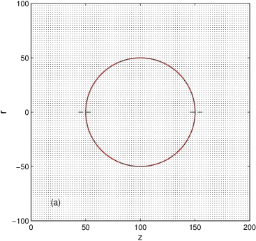
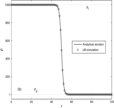
Figure 1: static droplet test with density ratio $\rho_{l}/\rho_{g}=1000$: (a) the velocity distribution of the whole domain at the equilibrium state and the solid and dashed lines respectively represent the equilibrium shape of the droplet and its initial shape; (b) density profile across the interface obtained from LB simulation and corresponding analytical solution.

Figure 1(a) depicts the steady droplet shape obtained by the present LB model, together with the initial one. It is found that they match to each other with a high accuracy. Further, we also plotted the numerical prediction of the density profile across the interface in Fig. 1(b), where the analytical solution given by Eq. (42) is as well presented for the comparison. It can be clearly observed that numerical result agrees well with the analytical solution, which indicates that the present model can correctly solve the phase interface. The existence of the spurious velocities is a common undesirable feature in many numerical methods for multiphase flows. If they have comparable magnitudes as the real fluid velocity, numerical instability or some unphysical phenomena could take place, and thus achieving small spurious velocities is very significative. The spurious velocities also rooted in the LB method arise from the imbalance between discrete forces in the interfacial region and cannot be totally eliminated to round-off in the framework of the LB approach [54]. We also displayed the spurious velocities generated by the present LB model. The distribution of the velocity field in the whole computational domain is shown in Fig. 1(a). It can be obviously found that the spurious velocities indeed exist in the vicinity of the interface, and the maximum magnitude of the spurious velocities computed by $|\textbf{u}|_{max}=(\sqrt{u^{2}+v^{2}})_{max}$ is about $1\times 10^{-6}$. We also compared the spurious velocities generated by different LB approaches. The axisymmetric color-gradient LB multiphase model proposed by Liu et al. [41] can only deal with multiphase flows with moderate density ratio and they reported that it can derive the spurious velocities at the level of $10^{-5}$. In addition, it is found that the maximum amplitude of spurious velocities in an improved pseudo-potential model [55] has the order of $10^{-3}$. In comparisons with these common LB models, we can conclude that the present phase-field based LB model can derive relatively low spurious velocities.

3.2 Droplet oscillation test

The droplet oscillation is a classic example that is widely used to validate axisymmetric multiphase LB model for simulating dynamic problem [35, 39, 40, 41]. The liquid droplet will exhibit oscillatory behavior, if it is initially distorted from equilibrium spherical shape into an elliptical one. We intend to compare the droplet oscillation frequency obtained from the LB simulation with the analytical solution reported by Miller and Scriven [56]. According to their analysis, the theoretical prediction for the oscillation frequency of the $n$th mode can be given by

$$\omega_{n}=\omega_{n}^{*}-0.5\alpha\sqrt{\omega_{n}^{*}}+0.25\alpha^{2},$$ (43)

where $\omega_{n}^{*}$ is Lamb’s natural resonance frequency,

$$\omega_{n}^{*}=\sqrt{\frac{n(n-1)(n+1)(n+2)}{R_{e}^{3}[n\rho_{g}+(n+1)\rho_{l}]}\sigma},$$ (44)

where $R_{e}$ is the radius of droplet at the equilibrium state. In Eq. (43), the parameter $\alpha$ is included to account for the viscosity contribution and is expressed by [56]

$$\alpha=\frac{(2n+1)^{2}\rho_{l}\rho_{g}\sqrt{\nu_{l}\nu_{g}}}{\sqrt{2}R_{e}[n\rho_{g}+(n+1)\rho_{l}](\rho_{l}\sqrt{\nu_{l}}+\rho_{g}\sqrt{\nu_{g}})}.$$ (45)

The mode of the oscillation is denoted by $n$, which is set to be 2 for an initial ellipsoidal shape considered here.

The initial computational setup consists of an ellipsoidal droplet with the half -axial and -radial lengths denoted by $R_{z}$ and $R_{r}$, placed in a domain with the size of $N_{z}\times N_{r}=300\times 150$. The boundary conditions are chosen as those in the static droplet test. To match this initial condition, the profile of the phase field variable is given by

$$\phi(z,r)=0.5+0.5\tanh\left[2R_{e}\frac{1-\sqrt{(z-z_{c})^{2}/R_{z}^{2}+(r-r_{c})^{2}/R_{r}^{2}}}{W}\right],$$ (46)

where $(z_{c},r_{c})=(150,0)$ is the center coordinate of ellipsoidal droplet, and the equilibrium droplet radius $R_{e}$ can be calculated as $(R_{r}^{2}R_{z})^{1/3}$ based on the mass conservation of the liquid droplet. The density ratios used in this test range from 10 and 100, and we find that the model is still stable for a very large density ratio of 1000. Considering a very low oscillation frequency at a large density ratio, it is generally measured difficultly, and thus the result in this case is not presented. Some remaining physical parameters in the simulation are fixed as $W=4$, $\sigma=0.3$, $M=0.01$, $\nu_{l}=\nu_{g}=0.1$, and the relaxation factors in the matrices $\textbf{S}^{f}$ and $\textbf{S}^{g}$ are set to be those in the last test.

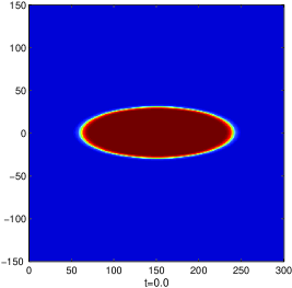
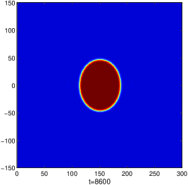
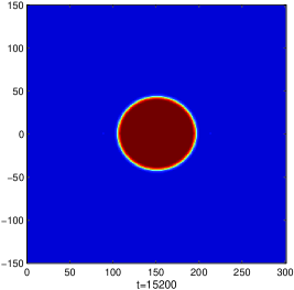
Figure 2: Evolution of the shape of an oscillating droplet with $\rho_{l}/\rho_{g}=100$, $R_{r}=30$, $R_{z}=90$, $\sigma=0.3$.

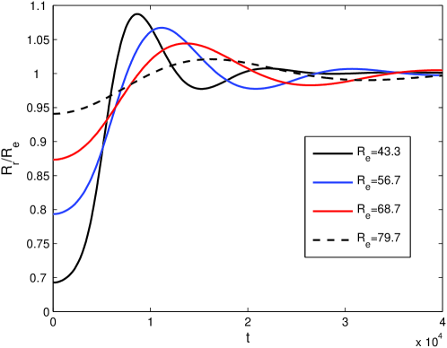
Figure 3: Time evolution of the half-axis length $R_{r}$ at different equilibrium radii with $\rho_{l}/\rho_{g}=100$, $\sigma=0.3$. And the half-axis length $R_{r}$ is normalized by the equilibrium radius $R_{e}$.

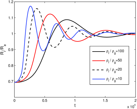
Figure 4: Time evolution of the half-axis length $R_{r}$ at different density ratios with $R_{r}=30$, $R_{z}=90$, $\sigma=0.3$. And the half-axis length $R_{r}$ is normalized by the equilibrium radius $R_{e}$.

Figure 2 shows the snapshots of an oscillating droplet at different times, where the density ratio is set as 100 and the initial droplet size is given by $R_{z}=90$ and $R_{r}=30$. As can be seen from Fig. 2, the droplet changes from a prolate shape at initial time to the oblate one at $t=8600$. Such change continues until the droplet reaches its equilibrium spherical shape. The above droplet behaviors are consistent with the expectation. We also conducted a quantitative study of droplet oscillation problem. The variation of the half-axis length $R_{r}$ versus time is plotted in Fig. 3, where the results with other initially given values of $R_{r}=45$, 60 and 75 are also presented to examine the effect of droplet size. It can be found from Fig. 3 that the amplitude of the oscillation normalized by the corresponding equilibrium radius $R_{e}$ fluctuates around 1 for all cases, and as expected, the dimensionless maximum amplitude is reduced for a larger droplet size. Further, from Fig. 3 we can compute the droplet oscillating frequency and showed the results in Table 1. For a comparison, the theoretical solution for predicting the oscillating frequency was also presented. It is found that they agree well in general, with the maximum relative error of around 8.9%.

Table 1: Comparison between the computed oscillating frequency $\omega_{LB}$ and corresponding analytical values $\omega_{ana}$ at different equilibrium radii for $\rho_{l}/\rho_{g}=100$, $\sigma=0.3$ and $R_{z}=90$.

$R_{e}$	43.3	56.7	68.7	79.7
$\omega_{LB}(\times 10^{-4})$	4.8934	3.4074	2.5964	2.1313
$\omega_{ana}(\times 10^{-4})$	5.3764	3.5864	2.6908	2.1533
$E_{r}=\frac{|\omega_{LB}-\omega_{ana}|}{\omega_{ana}}\times 100\%$	8.9%	5.0%	3.5%	5.7%

The influence of the density ratio on the oscillating frequency is also investigated here. We use the present model to simulate this case with four different density ratios $\rho_{l}/\rho_{g}=10$, 20, 50 and 100, and the droplet size is fixed to be $R_{z}=90$ and $R_{r}=30$. Figure 4 depicts the evolution of the oscillating amplitude with these typical density ratios. It can be clearly observed that the derived dimensionless amplitudes also fluctuates around 1, but the range is evidently reduced with the increase of the density ratio. In addition, the numerical predictions of the oscillating frequency obtained from the present LB model with various density ratios are summarized in Table 2, together with the corresponding analytical results. It can be seen that increasing density ratio decreases the droplet oscillating frequency, and the computed oscillating frequencies show good agreement with the analytical results for all density ratios, with a maximum error of about 8.9%.

Table 2: Comparison between the computed oscillating frequency $\omega_{LB}$ and corresponding analytical values $\omega_{ana}$ at different density ratios for $R_{z}=90$, $R_{r}=30$, and $\sigma=0.3$.

$\rho_{l}/\rho_{g}$	10	20	50	100
$\omega_{LB}(\times 10^{-4})$	15.2504	11.0000	7.0439	4.8934
$\omega_{ana}(\times 10^{-4})$	16.5854	12.0000	7.5895	5.3764
$E_{r}=\frac{|\omega_{LB}-\omega_{ana}|}{\omega_{ana}}\times 100\%$	8.0%	8.3%	7.2%	8.9%

3.3 Breakup of a liquid thread test

To show the capacity of the current model in simulating large interface topological changes, in the subsection we consider a fascinating problem of the breakup of a liquid thread into satellite droplets. The breakup of liquid filaments is of long-standing importance not only in its own interests, but also in the fact that numerous practical applications, such as gene chip arraying, ink-jet printing and microfluidics, depend critically on the knowledge of the breakup mechanisms [57, 58]. The earliest experimental study on the breakup of liquid filament was attributed to Plateau [59], and later Rayleigh [60] performed the linear stability analysis on this problem, who argued that a cylindrical liquid thread of radius $R$ is unstable, if the wavelength $\tilde{\lambda}$ of a disturbance on thread surface is longer than its circumference $2\pi R$. Usually, this instability criterion can also be described by using the wave number $k$, i.e., $k=2{\pi}R/\tilde{\lambda}$. When $k$ is smaller than 1, a liquid thread is unstable and can separate into small droplets, while it is stable for the case of $k>1$. Some preliminary numerical experiments with $k>1$ were first performed, and the breakup phenomena indeed cannot be observed in the simulations, which is in accordance with the linear theory. In the following, we restrict our attention to the breakup case, i.e., $k<1$, and compare the present numerical results with some available data.

The simulations were carried out in a $N_{z}\times N_{r}=\tilde{\lambda}\times 200$ lattice domain with the same boundary conditions used in the static and oscillating droplet tests. An initial disturbance imposed on thread surface is given by setting the phase field profile as

$$\phi(z,r)=0.5+0.5\tanh{\frac{2(R+d-r)}{W}},$$ (47)

where the radius $R$ is taken as 60, and $d$ is the perturbation function given by $d=0.1R\cos(2\pi z/\tilde{\lambda})$. To examine the wave number effect, several cases with different wavelengths $\tilde{\lambda}$=420, 500, 600, 800, 1000, 1200, 1800 were simulated, which correspond to various wave numbers $k$=0.90, 0.75, 0.63, 0.47, 0.38, 0.31, 0.21. In the simulations, two different density ratios of $\rho_{l}/\rho_{g}=100$ and 10 are considered and the interfacial tension $\sigma$ is fixed as 0.3. We would like to stress that the model can also tackle this case with a high density ratio of 1000, while it takes plenty of time for the system to reach the breakup state under the identical surface tension force. In this case, the moderate density ratio is merely considered. Here some other used physical parameters are given as $W=4.0$, $M=0.01$ and $\nu_{l}=\nu_{g}=0.1$. The parameters in both $\textbf{S}^{f}$ and $\textbf{S}^{g}$ are chosen as those in the last test.

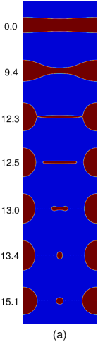
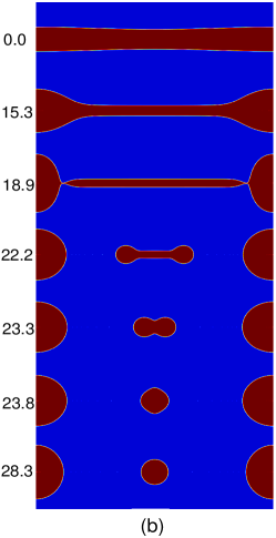
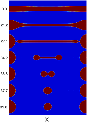
Figure 5: Evolutions of the breakup of a liquid thread at different wave numbers with the density ratio of $\rho_{l}/\rho_{g}=100$, (a) $k=0.63$, (b) $k=0.31$, (c) $k=0.21$. Time has been normalized by the capillary time $\sqrt{R^{3}\rho_{l}/\sigma}$.

We first present the results for the density ratio of 100. Figure 5 depicts the time evolution of a liquid thread with three typical wave numbers, where time has been normalized by the capillary time $\sqrt{R^{3}\rho_{l}/\sigma}$. It can be observed from Fig. 5 that for all cases, the interfacial perturbation grows continuously at early stage, and then the liquid thread in middle region becomes more and more thin, while its ends are enlarged with time. As time goes on, the liquid thread breaks up at two thin linking points, forming into a liquid ligament as well as a main droplet. Afterwards, the liquid ligament shrinks constantly with the action of the dominant surface tension, until it reaches an equilibrium spherical state. Lastly, a pair of liquid droplets including the main droplet and the satellite one can be observed in the system. Actually, the formed liquid ligament can be treat as the secondary liquid thread, and whether its breakup occurs or not depends on the new wavelength. If the wavelength is sufficiently large such that the instability criterion can be satisfied, the secondary breakup of the ligament can take place, leading to the formation of multiple satellite droplets. The above behaviors of the thread breakup obtained by the present model are qualitatively consistent with the previous studies [61, 62].

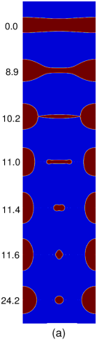
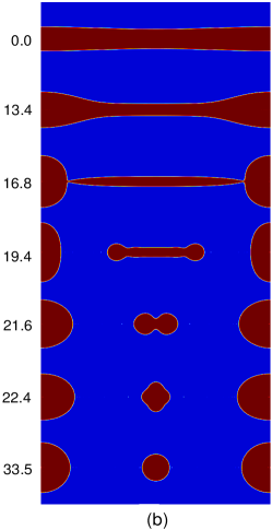
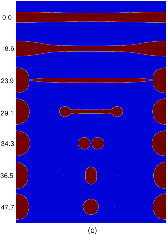
Figure 6: Evolutions of the breakup of a liquid thread at different wave numbers with the density ratio of $\rho_{l}/\rho_{g}=10$, (a) $k=0.63$, (b) $k=0.31$, (c) $k=0.21$. Time has been normalized by the capillary time $\sqrt{R^{3}\rho_{l}/\sigma}$.

To further investigate the density ratio effect, we also simulate the breakup of a liquid thread with the density ratio of $\rho_{l}/\rho_{g}=10$, where other physical parameters remain unchanged. The snapshots of the breakup of a liquid thread with three different wave numbers are shown in Fig. 6. It is found that compared with the case of $\rho_{l}/\rho_{g}=100$, the liquid thread exhibits similar behaviors at early time for all the wave numbers. The initial disturbance imposed on the thread surface increases in time, which then results in the formation of a thin ligament and a main droplet. Afterwards, some distinct behaviors of a liquid ligament are observed for different wave numbers. For the case of $k=0.62$ or 0.31, the filament contracts continuously into one satellite droplet. This phenomenon is a familiar spectacle in simulation results with the density ratio of 100. Whereas for the case of $k=0.21$, the liquid ligament shrinks at first, and then pinches off due to the Rayleigh instability, which leads to the relaxation of two daughter droplets. The two daughter droplets move toward each other, and eventually merge into a larger satellite droplet. These processes are the results of the inertia and surface tension action, and are in line with the results reported in literatures [40, 61, 62]. In contrast, the secondary breakup of the ligament does not occur for the density ratio of 100, which indicates that a higher density ratio prevents the interface rupture. Besides, the breakup time is a concerned physical quantity in the study of thread instability. We also measured the breakup time for two density ratios with various wave numbers. The computed breakup times for the density ratio of 100 at three wave numbers $k=0.63$, 0.31, 0.21 are 12.3, 18.9, 27.1, while they for the density ratio of 10 are 10.2, 16.8, 23.9. Therefore it is concluded that increasing density ratio can slow down the breakup of a liquid thread. Furthermore, we also give a quantitative study on the thread breakup, and showed in Fig. 7 the main and satellite droplet sizes with two density ratios and various wave numbers. For comparisons, some available literature results, including the finite element results of Ashgriz and Mashayek [61], the analytical solutions and experimental data of Lafrance [63], as well as the experimental data by Rutland and Jameson [64], are also presented. It can be seen that both the main and satellite droplet sizes decrease with the increasing wave number, and also, it is found that the satellite droplet size is reduced for a larger density ratio, whereas the trend is just the reverse for the main droplet due to the mass conservation. The numerical predictions for the droplet sizes obtained from the present LB simulations are further found to be in good agreement with these available date in general.

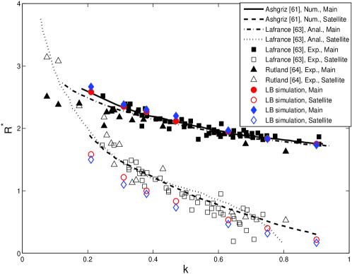
Figure 7: The terminal droplet sizes at different wave numbers. Here the red circle and blue rhombus respectively represent the cases of $\rho_{l}/\rho_{g}=10$ and $\rho_{l}/\rho_{g}=100$, and the droplet radius $R^{*}$ has been normalized by $R$.

4 Summary

Numerical modeling of axisymmetric multiphase flows with large density contrasts is still an intractable task in the framework of the LB method. In this paper, we propose a simple and efficient LB model for axisymmetric multiphase system, which is capable of handling large density differences. The proposed LB model is built upon the conservative phase-field equation, which involves a lower-order diffusion term as opposed to the widely used Cahn-Hilliard equation. Therefore the present model in theory can achieve better numerical stability and accuracy in solving phase interface than the Cahn-Hilliard type of axisymmetric LB models. Two LB evolution equations are utilized in the current model, one of which is used for capturing phase interface and the other for solving fluid velocity and pressure. A new equilibrium distribution function and some discrete source terms are designed in the LB equation for interface capturing. Meanwhile, a simpler forcing distribution function is also proposed in the LB equation for hydrodynamics. Different from most of previous axisymmetric LB multiphase models [35, 24, 36, 38, 39], the added source terms accounting for the axisymmetric effect contain no gradients in the present model. The present model is also equipped with an advanced MRT collision operator to enhance its numerical stability. We conducted the Chapman-Enskog analysis on the present MRT-LB equations, and it is demonstrated that both the conservative AC equation and the incompressible NS equations in the cylindrical coordinate system can be recovered correctly from the present model. To validate the present model, we first simulated a steady problem of the static droplet with a high density ratio of 1000, and it is found that the present model can accurately solve the density field, and also achieve low spurious velocities with the order of $10^{-6}$. To further assess the current model, two dynamic benchmark problems of a droplet oscillation and a liquid thread breakup are considered. It is shown that the present model can provide satisfactory predictions of the droplet oscillation frequency and the generated daughter droplet sizes for a board range of density ratios. At last, we simulated the realistic buoyancy-driven bubbly flow with a large density ratio of 1000. Some fascinating bubble dynamics are successfully reproduced by the present model, and the numerically predicted terminal bubble patterns show good agreements with the experimental date and some available numerical results. It is also reported that the present model can describe bubble interfacial dynamics with a higher accuracy than the existing axisymmetric LB model [24]. The present method is developed based on the standard orthogonal MRT model, and its extension to the non-orthogonal MRT one can be conducted directly. It is expected that the non-orthogonal model can retain the numerical accuracy while simplifying the implementation [69, 70]. In conclusion, we anticipate that our present numerical method will be useful for many practical and sophisticated problems.

Appendix A Chapman-Enskog analysis of axisymmetric LB model for the Allen-Cahn equation

The Chapman-Enskog analysis is now carried out to demonstrate the consistency of the LB evolution equation (9) with the axisymmetric AC equation. We first introduce the multiscaling expansions for the distribution function, time derivative, space gradient, and discrete source term as

$${{f}_{i}}={f}_{i}^{(0)}+\epsilon{f}_{i}^{(1)}+{\epsilon^{2}}{f}_{i}^{(2)}+\cdot\cdot\cdot,$$ (48a)

$${\partial_{t}}=\epsilon{\partial_{t_{1}}}+{\epsilon^{2}}{\partial_{t_{2}}},\nabla=\epsilon{\nabla_{1}},F_{i}=\epsilon{F_{i}}^{(1)}+\epsilon^{2}{F_{i}}^{(2)},$$ (48b)

where $\epsilon$ is a small expansion parameter. Applying Taylor expansion to Eq. (9) about x and $t$, one can derive the resulting continuous equation

$${D_{i}}{{f}_{i}}+{{{\delta_{t}}}\over 2}D_{i}^{2}{{f}_{i}}+\cdot\cdot\cdot=-{1\over{{\delta_{t}}}}{({{\bf{M}}^{-1}}{{\bf{S}}^{f}}{\bf{M}})_{ij}}({{f}_{j}}-{f}_{j}^{eq})+{F_{i}},$$ (49)

where $D_{i}=\partial_{t}+\textbf{c}_{i}\cdot\nabla$. Substituting the expansions into Eq. (A.2), we can obtain the following equations in consecutive order of the parameter $\epsilon$,

$${\epsilon^{0}}:\qquad f_{i}^{(0)}=f_{i}^{(eq)},$$ (50a)

$${\epsilon^{1}}:\qquad{D_{1i}}f_{i}^{(0)}=-{1\over{{\delta_{t}}}}{({{\bf{M}}^{-1}}{{\bf{S}}^{f}}{\bf{M}})_{ij}}f_{j}^{(1)}+{\left[{{{\bf{M}}^{-1}}({\rm\textbf{I}}-{{{{\bf{S}}^{f}}}\over 2}){\bf{M}}}\right]_{ij}}{{R_{j}}}^{(1)},$$ (50b)

$${\epsilon^{2}}:\qquad{\partial_{{t_{2}}}}f_{i}^{(0)}+{D_{1i}}f_{i}^{(1)}+{{{\delta_{t}}}\over 2}D_{1i}^{2}f_{i}^{(0)}=-{1\over{{\delta_{t}}}}{({{\bf{M}}^{-1}}{{\bf{S}}^{f}}{\bf{M}})_{ij}}f_{j}^{(2)}+{\left[{{{\bf{M}}^{-1}}({\rm\textbf{I}}-{{{{\bf{S}}^{f}}}\over 2}){\bf{M}}}\right]_{ij}}{R_{j}}^{(2)},$$ (50c)

in which ${D_{1i}}={\partial_{{t_{1}}}}+{{\bf{c}}_{i}}\cdot{\nabla_{1}}$. Rewriting Eqs. (A.3) in vector form and premultiplying the matrix M on both sides of them, we can derive the corresponding equations in the moment space

$${\epsilon^{0}}:\qquad{{\bf{m}}_{f}^{(0)}}={{\bf{m}}_{f}^{(eq)}},$$ (51a)

$${\epsilon^{1}}:\qquad{{\hat{\bf{D}}}_{1}}{{\bf{m}}_{f}^{(0)}}=-{{\bf{S}}^{f^{\prime}}}{{\bf{{m}}}_{f}^{(1)}}+({\rm\textbf{I}}-{{{{\bf{S}}^{f}}}\over 2}){\bf{M}}{{\bf{{R}}}^{(1)}},$$ (51b)

$${\epsilon^{2}}:\qquad{\partial_{{t_{2}}}}{{\bf{m}}_{f}^{(0)}}+{\hat{{\bf{D}}}_{1}}({\rm\textbf{I}}-{{\bf{S}}^{f}\over 2}){{\bf{{m}}}_{f}^{(1)}}+{{{\delta_{t}}}\over 2}{\hat{\textbf{D}}_{1}}({\rm\textbf{I}}-{{\bf{S}}^{f}\over 2}){\bf{M}}{{{\bf{R}}}^{(1)}}=-{{\bf{S}}^{f^{\prime}}}{{\bf{{m}}}_{f}^{(2)}}+({\rm\textbf{I}}-{{{{\bf{S}}^{f}}}\over 2}){\bf{M}}{{\bf{{R}}}^{(2)}},$$ (51c)

where ${{\bf{S}}^{f^{\prime}}}={{\bf{S}}^{f}}/\delta_{t}$, ${\hat{{\bf{D}}}_{1}}=\textbf{M}{\textbf{D}_{1}}\textbf{M}^{-1}$, ${{\bf{D}}_{1}}={\partial_{{t_{1}}}}{\rm\textbf{I}}+{\nabla_{1}}\cdot diag({{\bf{c}}_{0}},{{\bf{c}}_{1}},\cdot\cdot\cdot,{{\bf{c}}_{8}})$, ${\bf{{m}}}_{f}^{(1)}=(m_{f_{0}}^{(1)},m_{f_{1}}^{(1)},\cdot\cdot\cdot,m_{f_{8}}^{(1)})$ and Eq. (A3.b) has been used to derive the resulting equation (A.4c). Substituting Eq. (21) to Eq. (A.4b), we can obtain several equations related to the target governing equations,

$${\partial_{{t_{1}}}}(r\phi)+{\partial_{{z_{1}}}}(r\phi{u_{z}})+{\partial_{{r_{1}}}}(r\phi{u_{r}}+M\phi)=0,$$ (52a)

$${\partial_{{t_{1}}}}(r\phi{u_{z}})+{\partial_{{z_{1}}}}({c_{s}^{2}}r\phi)=-c{s_{3}^{f^{\prime}}}m_{f_{3}}^{(1)}+c(1-\frac{{s_{3}^{f}}}{2}){mR_{1}^{(1)}},$$ (52b)

$${\partial_{{t_{1}}}}(r\phi{u_{r}}+M\phi)+{\partial_{{r_{1}}}}({c_{s}^{2}}r\phi)=-c{s_{5}^{f^{\prime}}}m_{f_{5}}^{(1)}+c(1-\frac{{s_{5}^{f}}}{2}){mR_{2}^{(1)}}.$$ (52c)

Similarly, the substitution of Eq. (21) into Eq. (A.4c) yields

$${\partial_{{t_{2}}}}(r\phi)+{\partial_{{z_{1}}}}{c(1-\frac{{s_{3}^{f}}}{2})m_{f_{3}}^{(1)}}+{\partial_{{r_{1}}}}c(1-\frac{{s_{5}^{f}}}{2})m_{f_{5}}^{(1)}+\frac{\delta_{t}}{2}\partial_{z_{1}}c(1-\frac{{s_{3}^{f}}}{2}){mR_{1}^{(1)}}+\frac{\delta_{t}}{2}\partial_{r_{1}}c(1-\frac{{s_{5}^{f}}}{2}){mR_{2}^{(1)}}=0,$$ (53)

where the unknown $m_{f_{3}}^{(1)}$ and $m_{f_{5}}^{(1)}$ can be determined from Eqs. (A.5b-A.5c), and then their expressions can be given by

$$c{s_{3}^{f^{\prime}}}m_{f_{3}}^{(1)}=-{\partial_{{t_{1}}}}(r\phi{u_{z}})-{\partial_{{z_{1}}}}({c_{s}^{2}}r\phi)+c(1-\frac{{s_{3}^{f}}}{2}){mR_{1}^{(1)}},$$ (54a)

$$c{s_{5}^{f^{\prime}}}m_{f_{5}}^{(1)}=-{\partial_{{t_{1}}}}(r\phi{u_{r}}+M\phi)-{\partial_{{r_{1}}}}({c_{s}^{2}}r\phi)+c(1-\frac{{s_{5}^{f}}}{2}){mR_{2}^{(1)}}.$$ (54b)

Substituting Eqs. (A7) to Eq. (A6), we have

$$\partial_{t_{2}}(r\phi)=\partial_{z_{1}}c_{s}^{2}\delta_{t}(\frac{1}{s_{3}^{f}}-\frac{1}{2})\left[\partial_{z_{1}}(r\phi)-r\lambda n_{z}^{(1)}\right]+\partial_{r_{1}}c_{s}^{2}\delta_{t}(\frac{1}{s_{5}^{f}}-\frac{1}{2})\left[\partial_{r_{1}}(r\phi)-r\lambda n_{r}^{(1)}\right],$$ (55)

where Eq. (23) has been applied. Combining Eq. (A.5a) at $t_{1}$ time scale and Eq. (A.8) at $t_{2}$ time scale, we can derive the recovered equation,

$$\partial_{t}(r\phi)+\partial_{\alpha}(r\phi u_{\alpha}+M\phi\delta_{\alpha r})=\partial_{\alpha}(M\partial_{\alpha}r\phi)-M\partial_{\alpha}(r\lambda n_{\alpha}),$$ (56)

where the relation $s_{3}^{f}=s_{5}^{f}$ has been used to obtain the isotropic mobility,

$$M=c_{s}^{2}\delta_{t}(\frac{1}{s_{3}^{f}}-\frac{1}{2}).$$ (57)

From the above procedure, it is clear that the axisymmetric AC equation can be recovered correctly from the present MRT model without adopting any approximations.

Appendix B Chapman-Enskog analysis of axisymmetric LB model for the incompressible hydrodynamic equations

The present MRT-LB model for the axisymmetric NS equations is also analyzed by applying the Chapman-Enskog expansions, and similarly the particle distribution function, time and space derivatives, forcing distribution function can be expanded as

$${{g}_{i}}={g}_{i}^{(0)}+\epsilon{g}_{i}^{(1)}+{\epsilon^{2}}{g}_{i}^{(2)}+\cdot\cdot\cdot,$$ (58a)

$${\partial_{t}}=\epsilon{\partial_{t_{1}}}+{\epsilon^{2}}{\partial_{t_{2}}},\nabla=\epsilon{\nabla_{1}},G_{i}=\epsilon{G_{i}}^{(1)}.$$ (58b)

Adopting Taylor expansion to Eq. (24) and substituting the expansions (B.1) into the resulting equation, one can get the zero-, first-, and second-order equations in the parameter $\epsilon$,

$${\epsilon^{0}}:\qquad{g}_{i}^{(0)}={g}_{i}^{(eq)},$$ (59a)

$${\epsilon^{1}}:\qquad{D_{1i}}{g}_{i}^{(0)}=-{1\over{{\delta_{t}}}}{({{\bf{M}}^{-1}}{{\bf{S}}^{g}}{\bf{M}})_{ij}}{g}_{j}^{(1)}+{{G_{i}}}^{(1)},$$ (59b)

$${\epsilon^{2}}:\qquad{\partial_{{t_{2}}}}{g}_{i}^{(0)}+{D_{1i}}{g}_{i}^{(1)}+{{{\delta_{t}}}\over 2}D_{1i}^{2}{g}_{i}^{(0)}=-{1\over{{\delta_{t}}}}{({{\bf{M}}^{-1}}{{\bf{S}}^{g}}{\bf{M}})_{ij}}{g}_{j}^{(2)}.$$ (59c)

Substituting Eq. (B.2b) into Eq. (B.2c) and multiplying matrix M on the both sides of Eqs. (B2) separately gives

$${\epsilon^{0}}:\qquad{{\bf{m}}_{g}^{(0)}}={{\bf{m}}_{g}^{(eq)}},$$ (60a)

$${\epsilon^{1}}:\qquad{{\hat{\bf{D}}}_{1}}{{\bf{m}}_{g}^{(0)}}=-{{\bf{S}}^{g^{\prime}}}{{\bf{{m}}}_{g}^{(1)}}+({\rm\textbf{I}}-{{{{\bf{S}}^{g}}}\over 2}){\bf{M}}{{\bf{{T}}}^{(1)}},$$ (60b)

$${\epsilon^{2}}:\qquad{\partial_{{t_{2}}}}{{\bf{m}}_{g}^{(0)}}+{\hat{{\bf{D}}}_{1}}({\rm\textbf{I}}-{{\bf{S}}^{g}\over 2}){{\bf{{m}}}_{g}^{(1)}}+{{{\delta_{t}}}\over 2}{\hat{\textbf{D}}_{1}}({\rm\textbf{I}}-{{\bf{S}}^{g}\over 2}){\bf{M}}{{{\bf{T}}}^{(1)}}=-{{\bf{S}}^{g^{\prime}}}{{\bf{{m}}}_{g}^{(2)}},$$ (60c)

where ${{\bf{S}}^{g^{\prime}}}={{\bf{S}}^{g}}/\delta_{t}$. Now it is seen that the distribution functions in the discrete-velocity space can be projected onto the macroscopic quantities in the moment space. Based on the moment conditions, we can define ${{\bf{{m}}}_{g}}$ as

$${{\bf{{m}}}_{g}}={\bf{M}}{{\bf{g}}}=(-{{{\delta_{t}}}\over 2}{r}{\bf{u}}\cdot\nabla\rho,{{m}_{g_{1}}},{{m}_{g_{2}}},{{r\rho{u_{z}}}\over c}-{{{\delta_{t}}{F_{z}}}\over{2c}},{{m}_{g_{4}}},{{r\rho{u_{r}}}\over c}-{{{\delta_{t}}{F_{r}}}\over{2c}},{{m}_{g_{6}}},{{m}_{g_{7}}},{{m}_{g_{8}}})^{\rm T},$$ (61)

and ${{\bf{{m}}}_{g}^{(k)}}(k\geq 1)$ can be denoted by

$${{\bf{{m}}}_{g}^{(1)}}=(-{{{\delta_{t}}}\over 2}{r\bf{u}}\cdot{\nabla_{1}}\rho,{m}_{g_{1}}^{(1)},{m}_{g_{2}}^{(1)},-{{{\delta_{t}}{F_{z}}^{(1)}}\over{2c}},{m}_{g_{4}}^{(1)},-{{{\delta_{t}}{F_{r}}^{(1)}\over{2c}},{m}_{g_{6}}^{(1)}},{m}_{g_{7}}^{(1)},{m}_{g_{8}}^{(1)})^{\rm T},$$ (62a)

$${{\bf{{m}}}_{g}^{(k)}}=(0,{m}_{g_{1}}^{(k)},{m}_{g_{2}}^{(k)},0,{m}_{g_{4}}^{(k)},0,{m}_{g_{6}}^{(k)},{m}_{g_{7}}^{(k)},{m}_{g_{8}}^{(k)})^{\rm T},\qquad(k\geq 2).$$ (62b)

Substituting Eqs. (36-37) and Eq. (B.5a) into Eq. (B.3b), we can obtain several macroscopic equations at the $\epsilon$ scale, and only ones used to recover the hydrodynamic equations are presented here,

$${\partial_{{z_{1}}}}{(ru_{z})}+{\partial_{{r_{1}}}}{(ru_{r})}=0,$$ (63a)

$${\partial_{{t_{1}}}}(r\rho{u_{z}})+{\partial_{{z_{1}}}}(rp+r\rho u_{z}^{2})+{\partial_{{r_{1}}}}(r\rho{u_{z}}{u_{r}})=F_{z}^{(1)},$$ (63b)

$${\partial_{{t_{1}}}}(r\rho{u_{r}})+{\partial_{{z_{1}}}}r\rho{u_{z}}{u_{r}}+{\partial_{{r_{1}}}}(rp+r\rho u_{r}^{2})=F_{r}^{(1)},$$ (63c)

$${\partial_{{t_{1}}}}{{2rp+r\rho u_{z}^{2}+r\rho u_{r}^{2}}\over{c_{s}^{2}}}=-s_{1}^{g^{\prime}}{m}_{{g_{1}}}^{(1)}+{T_{{g_{1}}}},$$ (63d)

$${\partial_{{t_{1}}}}{{r\rho u_{z}^{2}-r\rho u_{r}^{2}}\over{{c^{2}}}}+{\partial_{{z_{1}}}}{{2r\rho{u_{z}}}\over 3}-{\partial_{{r_{1}}}}{{2r\rho{u_{r}}}\over 3}=-s_{7}^{g^{\prime}}{m}_{{g_{7}}}^{(1)}+{T_{{g_{7}}}},$$ (63e)

$${\partial_{{t_{1}}}}{{r\rho{u_{z}}{u_{r}}}\over{{c^{2}}}}+{\partial_{{z_{1}}}}{{r\rho{u_{r}}}\over 3}+{\partial_{{r_{1}}}}{{r\rho{u_{z}}}\over 3}=-s_{8}^{g^{\prime}}{m}_{{g_{8}}}^{(1)}+{T_{{g_{8}}}},$$ (63f)

where

$${T_{{g_{1}}}}=2(1-{{s_{1}^{g}}\over 2})(\rho{u_{r}}),$$ (64a)

$${T_{{g_{7}}}}={{2\over{{3}}}(1-{{s_{7}^{g}}\over 2})\left[{{u_{z}}{\partial_{z_{1}}}(r\rho)-{u_{r}}{\partial_{r_{1}}}(r\rho)}\right]},$$ (64b)

$${T_{{g_{8}}}}={{{1\over{{3}}}(1-{{s_{8}^{g}}\over 2})\left[{{u_{z}}{\partial_{r_{1}}}(r\rho)+{u_{r}}{\partial_{z_{1}}}(r\rho)}\right]}}.$$ (64c)

Similarly, we substitute Eqs. (36-37) and Eqs. (B.5) into Eq. (B.3c). With some algebraic operations, the moment equations at the $\epsilon^{2}$ scale can be derived and the related ones are presented as

$${\partial_{{t_{2}}}}(r\rho{u_{z}})+{{{c^{2}}}\over 6}{\partial_{{z_{1}}}}(1-{{s_{1}^{g}}\over 2}){m}_{g_{1}}^{(1)}+{{{c^{2}}}\over 2}{\partial_{{z_{1}}}}(1-{{s_{7}^{g}}\over 2}){m}_{g_{7}}^{(1)}+{c^{2}}{\partial_{{r_{1}}}}(1-{{s_{8}^{g}}\over 2}){m}_{g_{8}}^{(1)}+{T_{gz178}}=0,$$ (65a)

$${\partial_{{t_{2}}}}(r\rho{u_{r}})+{{{c^{2}}}\over 6}{\partial_{{r_{1}}}}(1-{{s_{1}^{g}}\over 2}){m}_{g_{1}}^{(1)}-{{{c^{2}}}\over 2}{\partial_{{r_{1}}}}(1-{{s_{7}^{g}}\over 2}){m}_{g_{7}}^{(1)}+{c^{2}}{\partial_{{z_{1}}}}(1-{{s_{8}^{g}}\over 2}){m}_{g_{8}}^{(1)}+{T_{gr178}}=0,$$ (65b)

where ${T_{gz178}}$ and ${T_{gr178}}$ are given by

$${T_{gz178}}={\partial_{{z_{1}}}}(1-{{s_{1}^{g}}\over 2}){{{{c^{2}}{\delta_{t}}}\over 6}{(\rho{u_{r}})}}+{\partial_{{z_{1}}}}(1-{{s_{7}^{g}}\over 2}){{{c^{2}}{\delta_{t}}}\over 6}{\left[{{u_{z}}{\partial_{z_{1}}}(r\rho)-{u_{r}}{\partial_{r_{1}}}(r\rho)}\right]}$$

$$+{\partial_{{r_{1}}}}(1-{{s_{8}^{g}}\over 2}){{{c^{2}{\delta_{t}}\over{{6}}}[{{u_{z}}{\partial_{r_{1}}}(r\rho)+{u_{r}}{\partial_{z_{1}}}(r\rho)}]}},$$ (66)

and

$${T_{gr178}}={\partial_{{r_{1}}}}(1-{{s_{1}^{g}}\over 2}){{{{c^{2}}{\delta_{t}}}\over 6}{(\rho{u_{r}})}}-{\partial_{{r_{1}}}}(1-{{s_{7}^{g}}\over 2}){{{c^{2}}{\delta_{t}}}\over 6}{[{{u_{z}}{\partial_{z_{1}}}(r\rho)-{u_{r}}{\partial_{r_{1}}}(r\rho)}]}$$

$$+{\partial_{{z_{1}}}}(1-{{s_{8}^{g}}\over 2}){{{{c^{2}}{\delta_{t}}\over{{6}}}[{{u_{z}}{\partial_{r_{1}}}(r\rho)+{u_{r}}{\partial_{z_{1}}}(r\rho)}]}},$$ (67)

In Eqs. (B.8), the variables ${m}_{g_{1}}^{(1)}$, ${m}_{g_{7}}^{(1)}$ and ${m}_{g_{8}}^{(1)}$ needs to be determined. Based on the relations (B.6), one can get

$$-s_{1}^{g^{\prime}}{m}_{{g_{1}}}^{(1)}={\partial_{{t_{1}}}}{{2rp+r\rho u_{z}^{2}+r\rho u_{r}^{2}}\over{c_{s}^{2}}}-2(1-{{s_{1}^{g}}\over 2})\rho{u_{r}},$$ (68a)

$$-s_{7}^{g^{\prime}}{m}_{{g_{7}}}^{(1)}={\partial_{{t_{1}}}}{{r\rho u_{z}^{2}-r\rho u_{r}^{2}}\over{c^{2}}}+{{s_{7}^{g}}\over{{3}}}\left[{{u_{z}}{\partial_{z_{1}}}(r\rho)-{u_{r}}{\partial_{r_{1}}}(r\rho)}\right]+{2\over 3}r\rho\left[{\partial_{{z_{1}}}}{u_{z}}-{\partial_{{r_{1}}}}{u_{r}}\right],$$ (68b)

$$-s_{8}^{g^{\prime}}{m}_{{g_{8}}}^{(1)}={\partial_{{t_{1}}}}{{r\rho u_{z}u_{r}}\over{c^{2}}}+{{s_{8}^{g}}\over{{6}}}\left[{{u_{z}}{\partial_{r_{1}}}(r\rho)+{u_{r}}{\partial_{z_{1}}}(r\rho)}\right]+{1\over 3}r\rho\left[{\partial_{{r_{1}}}}{u_{z}}+{\partial_{{z_{1}}}}{u_{r}}\right].$$ (68c)

Substituting Eqs. (B.11) into Eqs. (B.8) and using the incompressible limits [$\partial_{t_{1}}p=O(Ma^{2})$ and $\mathbf{u}^{2}=O(Ma^{2})$], we can ultimately derive the second-order equations in $\epsilon$,

$${\partial_{{t_{2}}}}(r\rho{u_{z}})-{\partial_{{z_{1}}}}r\nu\rho({\partial_{{z_{1}}}}{u_{z}}-{\partial_{{r_{1}}}}{u_{r}}-\frac{u_{r}}{r})-{\partial_{{r_{1}}}}r\nu\rho({\partial_{{r_{1}}}}{u_{z}}+{\partial_{{z_{1}}}}{u_{r}})=0,$$ (69a)

$${\partial_{{t_{2}}}}(r\rho{u_{r}})-{\partial_{{z_{1}}}}r\nu\rho({\partial_{{z_{1}}}}{u_{r}}+{\partial_{{r_{1}}}}{u_{z}})-{\partial_{{r_{1}}}}r\nu\rho({\partial_{{r_{1}}}}{u_{r}}-{\partial_{{z_{1}}}}{u_{z}}-\frac{u_{r}}{r})=0,$$ (69b)

where the terms with the order of $O(\delta_{t}Ma^{2})$ have been neglected, and the kinematic viscosity can be given by

$$\nu=c_{s}^{2}\delta_{t}(\tau_{g}-{1\over 2}),$$ (70)

where $1/\tau_{g}=s_{1}^{g}=s_{7}^{g}=s_{8}^{g}$. Substituting Eq. (B.6a) into Eqs. (B.12) and further combining Eqs.(B.6a-B.6c) and Eqs. (B.12a-B.12b) at $t_{1}$ and $t_{2}$ time scales, we can obtain the hydrodynamic equations,

$$\partial_{\alpha}(ru_{\alpha})=0,$$ (71a)

$$\partial_{t}(r\rho{u_{\beta}})+{\partial_{\alpha}}(r\rho{u_{\alpha}}u_{\beta})=-\partial_{\beta}(rp)+{\partial_{\alpha}}[r\nu\rho({\partial_{\alpha}}u_{\beta}+{\partial_{\beta}}u_{\alpha})]+{F_{\beta}}.$$ (71b)

From the above discussions, it is shown that our MRT-LB model can exactly recover the axisymmetric hydrodynamic equations under the incompressible limits.

Appendix C Calculation of the hydrodynamic pressure

Lastly, we give a discussion on the calculation of the hydrodynamic pressure $p$. Based on Eq. (25), we have

$$g_{0}^{(eq)}({\bf{x}},t)={{r({\omega_{0}}-1)}\over{c_{s}^{2}}}p({\bf{x}},t)+r\rho{s_{0}}({\bf{u}}({\bf{x}},t)),$$ (72)

which can be further recast as

$$g_{0}({\bf{x}},t)-[g_{0}({\bf{x}},t)-g_{0}^{(eq)}({\bf{x}},t)]={{r({\omega_{0}}-1)}\over{c_{s}^{2}}}p({\bf{x}},t)+r\rho{s_{0}}({\bf{u}}({\bf{x}},t)).$$ (73)

Expanding $g_{i}(\textbf{x}+\textbf{c}_{i}\delta_{t},t+\delta_{t})$ in Eq. (24) about $\bf{x}$ and $t$, we can easily derive

$${\delta_{t}}D_{i}{g_{i}}(\textbf{x},t)=-\left[{{\bf{M}}^{-1}}{{\bf{S}}^{g}}{\bf{M}}\right]_{ij}\left[g_{j}(\textbf{x},t)-g_{j}^{eq}(\textbf{x},t)\right]+\delta_{t}{G}_{i}(\textbf{x},t)$$ (74)

to the order of ${O}(\delta_{t}^{2})$. Premultiplying the matrix $\textbf{M}^{-1}{\textbf{S}^{g}}^{-1}\textbf{M}$ on both sides of Eq. (C.3), we can get

$${g_{i}}({\bf{x}},t)-g_{i}^{(eq)}({\bf{x}},t)=-{\delta_{t}}{({{\bf{M}}^{-1}}{{\bf{S}}^{g}}^{-1}{\bf{M}})_{ij}}{D_{j}}{g_{j}}({\bf{x}},t)+{\delta_{t}}{({{\bf{M}}^{-1}}{{\bf{S}}^{g}}^{-1}{\bf{M}})_{ij}}{G_{j}}({\bf{x}},t),$$ (75)

which indicates

$$g_{i}({\bf{x}},t)=g_{i}^{(eq)}({\bf{x}},t)+O({\delta_{t}}).$$ (76)

With the above approximate, we can rewrite Eq. (C.4) as

$${g_{i}}({\bf{x}},t)-g_{i}^{(eq)}({\bf{x}},t)=-{\delta_{t}}{({{\bf{M}}^{-1}}{{\bf{S}}^{g}}^{-1}{\bf{M}})_{ij}}{D_{j}}{g_{j}^{(eq)}}({\bf{x}},t)+{\delta_{t}}{({{\bf{M}}^{-1}}{{\bf{S}}^{g}}^{-1}{\bf{M}})_{ij}}{G_{j}}({\bf{x}},t).$$ (77)

Substituting Eqs. (36) and (37) into Eq. (C.6), and taking $i=0$, we can have

$${g_{0}}({\bf{x}},t)-g_{0}^{(eq)}({\bf{x}},t)=({{3{s_{1}^{g}}+2{s_{2}^{g}}}\over{3{c^{2}}{s_{1}^{g}}{s_{2}^{g}}}}){\delta_{t}}{{\partial rp}\over{\partial t}}+({{{s_{1}^{g}}+{s_{2}^{g}}}\over{3{c^{2}}{s_{1}^{g}}{s_{2}^{g}}}}){\delta_{t}}{{\partial(r\rho{\bf{u}}\cdot{\bf{u}})}\over{\partial t}}-{{{s_{1}^{g}}+{s_{2}^{g}}-{s_{1}^{g}}{s_{2}^{g}}}\over{2{s_{1}^{g}}{s_{2}^{g}}}}\cdot{\delta_{t}}\omega_{0}\rho u_{r}$$ (78)

to the order of ${O}(\delta_{t}^{2})$. Under the incompressible condition, $\partial_{t}p=O(Ma^{2})$ and $|\textbf{u}|=O(Ma)$ are satisfied, and then we can rewrite Eq. (C.7) as

$${g_{0}}({\bf{x}},t)-g_{0}^{(eq)}({\bf{x}},t)=-{{{s_{1}^{g}}+{s_{2}^{g}}-{s_{1}^{g}}{s_{2}^{g}}}\over{2{s_{1}^{g}}{s_{2}^{g}}}}\cdot{\delta_{t}}\omega_{0}\rho u_{r}+O({{\delta_{t}}^{2}}+\delta_{t}Ma^{2}).$$ (79)

Substituting Eq. (C.8) into Eq. (C.2) yields

$${r({{\omega_{0}}-1})\over{c_{s}^{2}}}p={{g_{0}}}-r\rho{s_{0}}({\bf{u}})+{{{s_{1}^{g}}+{s_{2}^{g}}-{s_{1}^{g}}{s_{2}^{g}}}\over{2{s_{1}^{g}}{s_{2}^{g}}}}\cdot{\delta_{t}}\omega_{0}\rho u_{r}$$ (80)

to the order of $O(\delta_{t}^{2}+{\delta_{t}}M{a^{2}})$. Considering the first component in Eq. (B.4), the zeroth-order moment of the distribution function can be defined by

$$\sum\limits_{i}{g_{i}}=-\frac{\delta_{t}}{2}{r}{\bf{u}}\cdot\nabla\rho,$$ (81)

and the hydrodynamic pressure $p$ can be evaluated as

$$p=\frac{c_{s}^{2}}{1-\omega_{0}}\left[\frac{1}{r}\sum_{i\neq 0}g_{i}+\frac{\delta_{t}}{2}\textbf{u}\cdot\nabla\rho+\rho s_{0}(\textbf{u})-{{{s_{1}^{g}}+{s_{2}^{g}}-{s_{1}^{g}}{s_{2}^{g}}}\over{2{s_{1}^{g}}{s_{2}^{g}}}}\cdot\frac{{\delta_{t}}\omega_{0}\rho u_{r}}{r}\right].$$ (82)

References

- [1] C. Hirt, B. Nichols, Volume of fluid (VOF) method for the dynamics of free boundaries, J. Comput. Phys. 39 (1981) 201-225.
- [2] S.O. Unverdi, G. Tryggvason, A front-tracking method for viscous, incompressible, multi-fluid flows, J. Comput. Phys. 100 (1992) 25-37.
- [3] M. Sussman, P. Smereka, S. Osher, A level set approach for computing solutions to incompressible two-phase flow, J. Comput. Phys. 114 (1994) 146-159.
- [4] D. M. Anderson, G. B. McFadden, and A. A. Wheeler, Diffuse-interface methods in fluid mechanics, Annu. Rev. Fluid Mech. 30 (1998) 139-165.
- [5] H. Ding, P. D. M. Spelt, and C. Shu, Diffuse interface model for incompressible two-phase flows with large density ratios, J. Comput. Phys. 226 (2007) 2078-2095.
- [6] D. Jacqmin, Calculation of two-phase Navier-Stokes flows using phase-field modeling, J. Comput. Phys. 155 (1999) 96-127.
- [7] Z. L. Guo, C. Shu, Lattice Boltzmann Method and its Applications in Engineering, World Scientific, 2013.
- [8] T. Krger, H. Kusumaatmaja, A. Kuzmin, O. Shardt, G. Silva, and E. M. Viggen, The lattice Boltzmann Method: Principles and Practice, Springer, 2016.
- [9] J. W. Cahn, J. E. Hilliard, Free energy of a nonuniform system. I. Interfacial free energy, J. Chem. Phys. 28 (1958) 258-267.
- [10] Y. Sun and C. Beckermann, Sharp interface tracking using the phase-field equation, J. Comput. Phys. 220 (2007) 626-653.
- [11] P. H. Chiu and Y. T. Lin, A conservative phase field method for solving incompressible two-phase flows, J. Comput. Phys. 230 (2011) 185-204.
- [12] A. K. Gunstensen, D. H. Rothman, S. Zaleski, and G. Zanetti, Lattice Boltzmann model of immiscible fluids, Phys. Rev. A 43 (1991) 4320-4327.
- [13] X. Shan and H. Chen, Lattice Boltzmann model for simulating flows with multiple phases and components, Phys. Rev. E 47 (1993) 1815-1819.
- [14] M. Swift, W. Osborn, and J. Yeomans, Lattice Boltzmann Simulation of Nonideal Fluids, Phys. Rev. Lett. 75 (1995) 830-833.
- [15] X. He, S. Chen, and R. Zhang, A lattice Boltzmann scheme for incompressible multiphase flow and its application in simulation of Rayleigh-Taylor instability, J. Comput. Phys. 152 (1999) 642-663.
- [16] T. Lee and C. L. Lin, A stable discretization of the lattice Boltzmann equation for simulation of incompressible two-phase flows at high density ratio, J. Comput. Phys. 206 (2005) 16-47.
- [17] H. Liang, B. C. Shi, Z. L. Guo, and Z. H. Chai, Phase-field-based multiple-relaxation-time lattice Boltzmann model for incompressible multiphase flows, Phys. Rev. E 89 (2014) 053320.
- [18] H. Liang, B. C. Shi, and Z. H. Chai, Lattice Boltzmann modeling of three-phase incompressible flows, Phys. Rev. E 93 (2016) 013308.
- [19] H. Liu, Q. J. Kang, C. R. Leonardi, S. Schmieschek, A. Narvez, B. D. Jones, J. R. Williams, A. J. Valocchi, and J. Harting, Multiphase lattice Boltzmann simulations for porous media applications, Comput. Geosci. 20 (2016) 777-805.
- [20] Q. Li, H. K. Luo, Q. J. Kang, Y. L. He, Q. Chen, and Q. Liu, Lattice Boltzmann methods for multiphase flow and phasechange heat transfer, Prog. Energy Combust. Sci. 52 (2016) 62-105.
- [21] M. R. Nobari, Y. J. Jan, G. Tryggvason, Head-on collision of drops-A numerical investigation, Phys. Fluids 8 (1996) 29-42.
- [22] K. N. Premnath, J. Abraham, Simulations of binary drop collisions with a multiple-relaxation-time lattice-Boltzmann model, Phys. Fluids 17 (2005) 122105.
- [23] J. Hua, J. Lou, Numerical simulation of bubble rising in viscous liquid, J. Comput. Phys. 222 (2007) 769-795.
- [24] H. B. Huang, J. J. Huang, X. Y. Lu, A mass-conserving axisymmetric multiphase lattice Boltzmann method and its application in simulation of bubble rising, J. Comput. Phys. 269 (2014) 386-402.
- [25] D. R. Link, S. L. Anna, D. A. Weitz, and H. A. Stone, Geometrically mediated breakup of drops in microfluidic devices, Phys. Rev. Lett. 92 (2004) 054503.
- [26] A. S. Utada, A. Fernandez-Nieves, H. A. Stone, and D. A. Weitz, Dripping to jetting transitions in coflowing liquid streams, Phys. Rev. Lett. 99 (2007) 094502.
- [27] M. Bussmann, S. Chandra, and J. Mostaghimi, Modeling the splash of a droplet impacting a solid surface, Phys. Fluids 12 (2000) 3121-3132.
- [28] C. Josseranda and S. Zaleskib, Droplet splashing on a thin liquid film, Phys. Fluids 15 (2003) 1650-1657.
- [29] I. Halliday, L. A. Hammond, C. M. Care, K. Good, and A. Stevens, Lattice Boltzmann equation hydrodynamics, Phys. Rev. E 64 (2001) 011208.
- [30] Y. Peng, C. Shu, Y.T. Chew, J. Qiu, Numerical investigation of flows in Czochralski crystal growth by an axisymmetric lattice Boltzmann method, J. Comput. Phys. 186 (2003) 295-307.
- [31] Z. L. Guo, H. F. Han, B. C. Shi, and C. G. Zheng, Theory of the lattice Boltzmann equation: Lattice Boltzmann model for axisymmetric flows, Phys. Rev. E 79 (2009) 046708.
- [32] Q. Li, Y. L. He, G. H. Tang, and W. Q. Tao, Improved axisymmetric lattice Boltzmann scheme, Phys. Rev. E 81 (2010) 056707.
- [33] L. Zheng, Z. L. Guo, B. C. Shi, C. G. Zheng, Kinetic theory based lattice Boltzmann equation with viscous dissipation and pressure work for axisymmetric thermal flows, J. Comput. Phys. 229 (2010) 5843-5856.
- [34] L. Zhang, S. Yang, Z. Zeng, J. Chen, L. Wang, J.W. Chew, Alternative extrapolation-based symmetry boundary implementations for the axisymmetric lattice Boltzmann method, Phys. Rev. E 95 (2017) 043312.
- [35] K. N. Premnath, J. Abraham, Lattice Boltzmann model for axisymmetric multiphase flows, Phys. Rev. E 71 (2005) 056706.
- [36] S. Mukherjee, J. Abraham, Lattice Boltzmann simulations of two-phase flow with high density ratio in axially symmetric geometry, Phys. Rev. E 75 (2007) 026701.
- [37] Q. Lou, Z. L. Guo, and B. C. Shi, Effects of force discretization on mass conservation in lattice Boltzmann equation for two-phase flows, Europhys. Lett. 99 (2012) 64005.
- [38] J. J. Huang, H. B. Huang, C. Shu, Y. T. Chew, and S. L. Wang, Hybrid multiple-relaxation-time lattice-Boltzmann finite-difference method for axisymmetric multiphase flows, J. Phys. A: Math. Theor. 46 (2003) 055501.
- [39] S. Srivastava, P. Perlekar, J. H. M. ten Thije Boonkkamp, N. Verma, and F. Toschi, Axisymmetric multiphase lattice Boltzmann method, Phys. Rev. E 88 (2013) 013309.
- [40] H. Liang, Z. H. Chai, B. C. Shi, Z. L. Guo, and T. Zhang, Phase-field-based lattice Boltzmann model for axisymmetric multiphase flows, Phys. Rev. E 90 (2014) 063311.
- [41] H. Liu, L. Wu, Y. Ba, G. Xi, Y. Zhang. A lattice Boltzmann method for axisymmetric multicomponent flows with high viscosity ratio, J. Comput. Phys. 327 (2016) 873-893.
- [42] H. L. Wang, Z. H. Chai, B. C. Shi, H. Liang, Comparative study of the lattice Boltzmann models for Allen-Cahn and Cahn-Hilliard equations, Phys. Rev. E 94 (2016) 033304.
- [43] A. Fakhari and D. Bolster, Diffuse interface modeling of three-phase contact line dynamics on curved boundaries: A lattice Boltzmann model for large density and viscosity ratios, J. Comput. Phys. 334 (2017) 620-638.
- [44] Z. H. Chai, D. K Sun, H. L. Wang, B. C. Shi, A comparative study of local and nonlocal Allen-Cahn equations with mass conservation, Int. J. Heat Mass Tran. 122 (2018) 631-642.
- [45] H. Liang, J. R. Xu, J. X. Chen, H. L. Wang, Z. H. Chai, and B. C. Shi, Phase-field-based lattice Boltzmann modeling of large-density-ratio two-phase flows, Phys. Rev. E 97 (2018) 033309.
- [46] F. Ren, B. Song, M. C. Sukop, and H. Hu, Improved lattice Boltzmann modeling of binary flow based on the conservative Allen-Cahn equation, Phys. Rev. E 94 (2016) 023311.
- [47] J. Kim, A continuous surface tension force formulation for diffuse-interface models, J. Comput. Phys. 204 (2005) 784-804.
- [48] P. Lallemand and L. S. Luo, Theory of the lattice Boltzmann method: Dispersion, dissipation, isotropy, Galilean invariance, and stability, Phys. Rev. E 61 (2000) 6546-6562.
- [49] I. Ginzburg, F. Verhaeghe, and D. d’Humires, Two-relaxation-time lattice Boltzmann scheme: About parametrization, velocity, pressure and mixed boundary conditions, Commun. Comput. Phys. 3 (2008) 427-478.
- [50] Y. H. Qian, D. d’Humires, and P. Lallemand, Lattice BGK models for Navier-Stokes equation, Europhys. Lett. 17 (1992) 479-484.
- [51] M.A. Mazloomi, S.S. Chikatamarla, I.V. Karlin, Entropic lattice Boltzmann method for multiphase flows, Phys. Rev. Lett. 114 (2015) 174502.
- [52] Y. K. Wei, Z. D. Wang, H. S. Dou, and Y. H. Qian, A novel two-dimensional coupled lattice Boltzmann model for incompressible flowin application of turbulence Rayleigh-Taylor instability, Comput. Fluids 156 (2017) 97-102.
- [53] Z. L. Guo, C. G. Zheng, and B. C. Shi, Discrete lattice effects on the forcing term in the lattice Boltzmann method, Phys. Rev. E 65 (2002) 046308.
- [54] Z. L. Guo, C. G. Zheng, and B. C. Shi, Force imbalance in lattice Boltzmann equation for two-phase flows, Phys. Rev. E 83 (2011) 036707.
- [55] Z. Yu and L. S. Fan, Multirelaxation-time interaction-potentialbased lattice Boltzmann model for two-phase flow, Phys. Rev. E 82 (2010) 046708.
- [56] C. A. Miller, L. E. Scriven, The oscillations of a fluid droplet immersed in another fluid, J. Fluid Mech. 32 (1968) 417-435.
- [57] J. Eggers, Nonlinear dynamics and breakup of free-surface flows, Rev. Mod. Phys. 69 (1997) 865-929.
- [58] H. Wijshoff, The dynamics of the piezo inkjet printhead operation, Phys. Rep. 491 (2010) 77-177.
- [59] J. Plateau, Experimental and Theoretical Statics of Liquid Fluids Subject to Molecular Forces Only, vol. 1, Gauthier-Villars, Paris, 1873.
- [60] L. Rayleigh, On the instability of jets, Proc. Lond. Math. Soc. 10 (1878) 4-13.
- [61] N. Ashgriz, F. Mashayek, Temporal analysis of capillary jet breakup, J. Fluid Mech. 291 (1995) 163-190.
- [62] M. Tjahjadi, H. A. Stone, J. M. Ottino, Satellite and subsatellite formation in capillary breakup, J. Fluid Mech. 243 (1992) 297-317.
- [63] P. Lafrance, Nonlinear breakup of a laminar liquid jet, Phys. Fluids 18 (1975) 428-432.
- [64] D. F. Rutland, G. J. Jameson, Theoretical prediction of the sizes of drops formed in the breakup of capillary jets, Chem. Eng. Sci. 25 (1970) 1689-1698.
- [65] D. Bhaga, M. E. Weber, Bubbles in viscous liquids: shapes, wakes and velocities, J. Fluid Mech. 105 (1981) 61-85.
- [66] R. F. Mudde, Gravity-driven bubbly flows, Annu. Rev. Fluid Mech. 37 (2005) 393-423.
- [67] A. Gupta, R. Kumar, Lattice Boltzmann simulation to study multiple bubble dynamics, Int. J. Heat Mass Transf. 51 (2008) 5192-5203.
- [68] L. Amaya-Bower, T. Lee, Single bubble rising dynamics for moderate Reynolds number using lattice Boltzmann method, Comput. Fluids 39 (2010) 1191-1207.
- [69] A. De Rosis, Nonorthogonal central-moments-based lattice Boltzmann scheme in three dimensions, Phys. Rev. E 95 (2017) 013310.
- [70] A. De Rosis, Alternative formulation to incorporate forcing terms in a lattice Boltzmann scheme with central moments, Phys. Rev. E 95 (2017) 023311.