Constrained correlated-Gaussians for hyperspherical calculations

Abstract

We formulate a hyperspherical approach within standard configuration interaction calculations aiming at a description of large-scale dynamics of $N$-particle system. The channel wave function and the adiabatic channel energy are determined by solving a hyperradius-constrained eigenvalue problem of the adiabatic Hamiltonian. The needed matrix elements are analytically evaluated using correlated Gaussians with good orbital angular momentum and parity. The feasibility of the approach is tested in three-$\alpha$ system. A spectrum of the adiabatic channel energies is determined depending on the degree of localization of the basis functions.

I Introduction

The hyperspherical coordinate system is a natural extension of the three-dimensional spherical polar coordinates to a set of $N$-particle coordinates. The hyperspherical approach attempts to solve an $N$-particle Schrödinger equation by expressing the total wave function as a product of the hyperradial and hyperangular parts and can be used to solve bound and continuum state problems.

The main advantage of the hyperspherical method is that it provides a unified framework to describe quantum dynamics of complex reactions such as decay, fusion or fission. In other methods the choice of relevant coordinates is not trivial. For example, in nuclear fusion initially the relative distance between the nuclei might be the most important coordinate, but later other coordinates will be more suitable and necessary. In the hyperspherical approach the hyperradius captures all features of the complicated dynamical processes and describe dynamical properties of the system emerging at different hyperradial distances.

Two realizations of the hyperspherical approach are widely used (see Refs. zhukov93 ; lin95 ; krivec98 ; nielsen01 ; greene17 for reviews on the hyperspherical approach and its applications). In one approach the hyperangular part is expanded in terms of the hyperspherical harmonics that are eigenfunctions of the hyperangular kinetic-energy operator, and a coupled hyperradial equation is solved by including the interaction of the particles. In another approach, often called the adiabatic hyperspherical approach, the adiabatic Hamiltonian consisting of the hyperangular kinetic energy and the interaction potential is diagonalized first to obtain the adiabatic channel energies and channel wave functions. The total wave function is then expanded in terms of the basis set of the adiabatic channel wave functions. The adiabatic channel energies give hints on how the system responds as a function of hyperradial distances.

The advantage of the first approach is that the hyperspherical harmonics are known, but two difficulties may hinder the application. One problem is that convergence of the hyperspherical harmonics expansion is slow even for short-range potentials thompson00 , and it becomes prohibitively slow when a long-range potential, like the Coulomb coupling potential, acts at large hyperradial distances. This slowness is related to the fact that the hyperangular kinetic energy and the interaction potential do not commute macek68 ; kvitsinsky91 . The slow convergence causes huge discrepancies, e.g. in the triple-$\alpha$ reaction rate at low temperatures nguyen13 ; ishikawa13 ; suno16 ; suno15 . Another problem is that solving the coupled differential equation in the hyperradial coordinate may become hard when a number of avoided crossings occur in the potential energy curves.

Although the basic idea of the hyperpsherical method is not limited to three-body systems, its extension to more-particle system is impeded by the lack of appropriate basis functions that can be flexibly used in the hyperspherical calculation. References barnea00 ; barnea03 ; barnea10 ; bacca12 ; timofeyuk02 ; timofeyuk08 ; gattobigio11 discuss recent developments in going beyond the three-body problems.

In both realization of the hyperspherical approach, one calculates the matrix element of an operator ${\cal O}$,

$$\langle\Psi^{\prime}|{\cal O}|\Psi\rangle_{\rho=R},$$ (1)

where $\langle\ldots\rangle_{\rho=R}$ indicates that the matrix element is to be evaluated by integrating in all the coordinates but the hyperradius $\rho$, which is fixed to $R$. The integral of type (1) is hard to evaluate in general because specifying the hyperangle coordinates for the $N$-particle system is considerably involved and integrating in those coordinates requires many-dimensional integrations. Although some progress has recently been made with correlated Gaussian (CG) basis functions stecher09 ; rittenhouse11 ; rakshit12 ; daily14 , the total orbital angular momentum is limited to $L=0$ and 1.

In this paper we will examine the possibility of using the CG as suitable basis functions in hyperspherical calculations. The CG proposed many years ago boys60 ; singer60 is extended to describe motion with non-zero total orbital angular momentum, especially with the help of the global vector representation varga95 ; book ; suzuki98 . Together with the stochastic variational method varga94 ; varga95 ; book to select efficiently the parameters of the CG, many problems have accurately been solved with the CG. See, e.g. Refs. mitroy13 ; horiuchi14 ; mikami14 for some recent applications of CG.

We attempt to formulate the hyperspherical approach in standard configuration interaction calculations. Following the spirit of the second realization of the hyperspherical approach, we set up a number of basis functions that are expected to be important at $\rho\approx R$, calculate the matrix elements of the adiabatic Hamiltonian using the full coordinate integration instead of Eq. (1), and determine both the channel wave function and the adiabatic channel energy at $\rho\approx R$ by solving a hyperradius-constrained eigenvalue equation. We show that this scheme can be achieved using the CG basis functions. The emphasis of this paper is not on solving a specific problem with the hyperspherical approach but on carefully examining its feasibility and discussing problems that may occur.

We present our formulation in Sec. II, and show in Sec. III how to evaluate the needed matrix elements. In Sec. IV we test our method in three-$\alpha$ system that is the simplest possible system but contains all the complexities nevertheless. Section V is a summary and discussions.

II Schrödinger equation in hyperspherical approach

II.1 Hyperspherical coordinates

Let $\bm{r}_{i}\,(i=1,\ldots,N)$ denote the position coordinate of the $i$th particle. The mass $m$ of all particles is assumed to be the same, although the case of unequal mass can be treated by defining mass-scaled coordinates. We define a set of relative coordinates, $\bm{x}_{i}\ (i=1,\ldots,N-1)$,

$$\bm{x}_{i}=\sqrt{\frac{i}{i+1}}\Big{(}\bm{r}_{i+1}-\frac{1}{i}\sum_{j=1}^{i}\bm{r}_{j}\Big{)}.$$ (2)

The set $\bm{x}_{i}$ together with the center of mass (c.m.) coordinate, $\bm{x}_{N}\equiv{\bm{R}}_{\rm cm}=\sum_{i=1}^{N}{\bm{r}}_{i}/N$, defines a transformation matrix $U$ from the single-particle coordinates to the relative and c.m. coordinates:

$$\bm{x}_{i}=\sum_{j=1}^{N}U_{ij}\bm{r}_{j}\ \ (i=1,\ldots,N).$$ (3)

Conversely, $\bm{r}_{i}$ is expressed as $\bm{r}_{i}=\sum_{j=1}^{N}{U^{-1}}_{ij}\bm{x}_{j}$.

The square of the hyperradius $\rho$ is defined by

$$\rho^{2} =\sum_{i=1}^{N}(\bm{r}_{i}-\bm{R}_{\rm cm})^{2}=\frac{1}{N}\sum_{j>i=1}^{N}(\bm{r}_{i}-\bm{r}_{j})^{2},$$ (4)

which is equal to

$$\rho^{2}=\sum_{i=1}^{N-1}\bm{x}_{i}^{2}.$$ (5)

Let $\Omega$ denote a set of the hyperangle coordinates constructed from dimensionless coordinates, $\bm{\xi}_{i}=\bm{x}_{i}/\rho\ (i=1,\ldots,N-1)$. They are constrained as $\sum_{i=1}^{N-1}\bm{\xi}_{i}^{2}=1$. The volume element for integration excluding ${\bm{R}}_{\rm cm}$ is

$$d\bm{x}\equiv d\bm{x}_{1}\ldots d\bm{x}_{N-1}=\rho^{d-1}d\rho d\Omega,$$ (6)

where

$$d=3(N-1)$$ (7)

is the degree of freedom excluding the c.m. motion.

Since $\rho^{2}/N$ is the mean-square-radius operator, $\rho$ measures the global size of the system. Or $\rho$ is a kind of collective coordinate responding to a large-scale change of the system suzuki15 . Suppose that the system develops into $f$ subsystems or clusters, each of which consists of $N_{i}$ particles ($\sum_{i=1}^{f}N_{i}=N$). $\rho^{2}$ is rewritten as

$$\rho^{2}=\sum_{i=1}^{f}\rho_{i}^{2}+\rho_{\rm rel}^{2}$$ (8)

with

$$\rho_{i}^{2}=\sum_{j=1}^{N_{i}}({\bm{r}}_{(i-1)+j}-{\bm{R}}_{i})^{2},\ \ \ \rho_{\rm rel}^{2}=\sum_{i=1}^{f}N_{i}({\bm{R}}_{i}-{\bm{R}}_{\rm cm})^{2},$$ (9)

where $(i-1)=\sum_{k=1}^{i-1}N_{k}$ with $(0)=0$, and ${\bm{R}}_{i}$ is the c.m. coordinate of the $i$th cluster. $\rho_{i}$ is the hyperradius of the $i$th cluster, and $\rho_{\rm rel}$ stands for the hyperradius that measures the spatial extension of the relative motion of the clusters. In such phenomena that include the formation of $f$ subsystems, the contribution of $\sum_{i=1}^{f}\rho_{i}^{2}$ to $\rho^{2}$ remains finite, whereas $\rho^{2}_{\rm rel}$ takes an increasingly large value as $\rho$ increases. Moreover, since $\rho^{2}$ is invariant with respect to the number of clusters $f$, the hyperspherical coordinates have the unique advantage that they can treat any decomposition of the system in a unified way.

II.2 Equation of motion in hyperspherical approach

The Hamiltonian $H$ of the system consists of the kinetic energy $T$ and the interaction potential $V$:

$$H=T+V.$$ (10)

With the c.m. kinetic energy being subtracted, $T$ reads

$$T=-\frac{\hbar^{2}}{2m}\sum_{i=1}^{N-1}\frac{\partial^{2}}{\partial\bm{x}_{i}^{2}},$$ (11)

and it is separated into hyperradial ($T_{\rho}$) and hyperangular ($T_{\Omega}$) parts, $T=T_{\rho}+T_{\Omega}$:

$$T_{\rho}=-\frac{\hbar^{2}}{2m}\Big{(}\frac{\partial^{2}}{\partial\rho^{2}}+\frac{d-1}{\rho}\frac{\partial}{\partial\rho}\Big{)},\ \ \ T_{\Omega}=\frac{\hbar^{2}\Lambda^{2}}{2m\rho^{2}},$$ (12)

where $\Lambda^{2}$ is the squared grand angular momentum operator that can in principle be expressed in terms of the hyperangle coordinates and their derivatives. The adiabatic Hamiltonian

$$H_{\Omega}=T_{\Omega}+V$$ (13)

is a kind of a generalized potential. As usual, $V$ and consequently $H_{\Omega}$ is assumed to contain no derivative operator with respect to $\rho$.

Let the total wave function $\Psi^{JM\pi}$ of the system be labeled by the total angular momentum $J$, its $z$ component $M$, the parity $\pi$. The Schrödinger equation, $H\Psi^{JM\pi}=E^{J\pi}\Psi^{JM\pi}$, reads as

$$(T_{\rho}+H_{\Omega})\Psi^{JM\pi}=E^{J\pi}\Psi^{JM\pi}.$$ (14)

The channel wave function $\Phi_{\nu}^{JM\pi}(\rho,\Omega)$ and the adiabatic channel energy (or adiabatic potential) $U_{\nu}^{J\pi}(\rho)$ are defined by solving the eigenvalue problem of $H_{\Omega}$,

$$H_{\Omega}\Phi_{\nu}^{JM\pi}(\rho,\Omega)=U_{\nu}^{J\pi}(\rho)\Phi_{\nu}^{JM\pi}(\rho,\Omega).$$ (15)

In order to exploit the fact that $\rho$ can be treated as a $c$-number in Eq. (15), we need the matrix element $\langle\Phi_{\nu}^{JM\pi}|H_{\Omega}|\Phi_{\nu^{\prime}}^{JM\pi}\rangle_{\rho=R}$. Since its evaluation is, however, hard as already mentioned, we take a different route.

We set up a number of independent basis functions $\Phi^{JM\pi}_{l}\ (l=1,\ldots,M)$ that satisfy

$$\langle\Phi^{JM\pi}_{l}|\rho^{2}|\Phi^{JM\pi}_{l}\rangle=R^{2},$$ (16)

and assume that the $\nu$th ‘channel wave function’ $\Phi^{JM\pi}_{R\nu}$ at $\langle\rho^{2}\rangle=R^{2}$ is given as a combination of the basis functions

$$\Phi^{JM\pi}_{R\nu}=\sum_{l=1}^{M}c^{J\pi}_{R\nu,l}\Phi^{JM\pi}_{l}.$$ (17)

The coefficients $c^{J\pi}_{R\nu,l}$ are determined by solving the constrained eigenvalue problem

$$\langle\Phi^{JM\pi}_{l}|H_{\Omega}-U_{\,R\nu}^{J\pi}|\Phi^{JM\pi}_{R\nu}\rangle=0\ \ \ (l=1,\ldots,M),$$ (18)

subject to

$$\langle\Phi^{JM\pi}_{R\nu}|\rho^{2}|\Phi^{JM\pi}_{R\nu}\rangle=R^{2}.$$ (19)

Both $\Phi^{JM\pi}_{l}$ and $\Phi^{JM\pi}_{R\nu}$ are normalized, and the matrix elements in Eqs. (16), (18), and (19) are evaluated by integrating in all the coordinates. Appendix A shows how to determine the adiabatic channel energies $U^{J\pi}_{R\nu}$ at $R$ and mutually orthogonal channel wave functions $\Phi^{JM\pi}_{R\nu}$.

We calculate the channel wave functions at a number of mesh points $R_{i}$ and assume the total wave function to be approximated by their combinations

$$\Psi^{JM\pi}=\sum_{i\nu}\chi^{J\pi}_{i\nu}\Phi^{JM\pi}_{R_{i}\nu}.$$ (20)

Equation (14) reduces to the following equation for $\chi^{J\pi}_{i\nu}$:

$$\sum_{j\nu^{\prime}}\langle\Phi^{JM\pi}_{R_{i}\nu}|T_{\rho}+H_{\Omega}-E^{J\pi}|\Phi^{JM\pi}_{R_{j}\nu^{\prime}}\rangle\chi^{J\pi}_{j\nu^{\prime}}=0$$

$$\qquad\qquad\qquad\qquad\qquad\qquad{\rm for\ all}\ i\ {\rm and}\ \nu.$$ (21)

The condition (16) is necessary to look for a suitable basis set at $R$ because each piece of $H_{\Omega}$ shows different $\rho$-dependence and hence such set may change depending on $\rho$. Short-ranged interactions in $V$ become important in the region of small $\rho$, while long-ranged interactions like the Coulomb potential contribute at large $\rho$ as well. $T_{\Omega}$ is also long-ranged. Moreover, since the Coulomb potential and $T_{\Omega}$ do not commute each other, one has to take account of both terms simultaneously macek68 .

As a measure of the localization of a wave function $\Phi$, we introduce the standard deviation $\sigma$ of $\rho^{2}$:

$$\sigma^{2}=\frac{\langle\Phi|(\rho^{2}-\langle\Phi|\rho^{2}|\Phi\rangle)^{2}|\Phi\rangle}{\langle\Phi|\rho^{2}|\Phi\rangle^{2}}=\frac{\langle\Phi|\rho^{4}|\Phi\rangle}{\langle\Phi|\rho^{2}|\Phi\rangle^{2}}-1.$$ (22)

$\Phi^{JM\pi}_{R\nu}$ is obtained as a combination of $\Phi^{JM\pi}_{l}$s. Therefore, even though $\Phi^{JM\pi}_{l}$s are all set to have $\sigma$’s within a certain range, it may happen that the $\sigma$ value of $\Phi^{JM\pi}_{R\nu}$ is far beyond its range. To obtain $U_{\,R\nu}^{J\pi}$ around $\rho\approx R$, it is useful to check the $\sigma$ value of $\Phi^{JM\pi}_{R\nu}$. We will discuss this problem later.

Once $\Phi^{JM\pi}_{R_{i}\nu}$s are determined at $R_{i}$’s, Eq. (21) can be solved in a standard linear algebra. Note that the matrix element of $T_{\rho}$ is already available at the stage of solving the eigenvalue problem of $H_{\Omega}$. This is in sharp contrast to the standard hyperspherical method where no hyperradial function is employed and thus one has to use numerical differentiations with respect to $\rho$ or e.g. slow variable discretization method tolstikhin96 ; suno11 .

In what follows we omit the superscripts $JM\pi$.

III Correlated Gaussian as hyperspherical basis function

III.1 Correlated Gaussian and its generating function

We adopt the CG as the basis function. We use matrix notations to make equations compact. For example, $\bm{x}$ denotes a column vector of dimension $(N-1)$ whose $i$th element is $\bm{x}_{i}$. A tilde symbol $\widetilde{\ \ \ }$ indicates a transpose of a column vector or a matrix, e.g. $\widetilde{\bm{x}}$ is the row vector and $\rho^{2}$ may be written as $\widetilde{\bm{x}}\bm{x}$, where the scalar product of 3-dimensional vectors is implicitly understood: $\widetilde{\bm{x}}\bm{x}=\sum_{i=1}^{N-1}{\bm{x}}_{i}\cdot{\bm{x}}_{i}=\sum_{i=1}^{N-1}{\bm{x}}_{i}^{2}$.

The CG with the total orbital angular momentum $L$ and its $z$ component $M$ reads

$$f^{uA}_{KLM}(\bm{x})={\cal N}^{uA}_{KL}|\widetilde{u}\bm{x}|^{2K+L}Y_{LM}(\widehat{\widetilde{u}\bm{x}})e^{-\frac{1}{2}\widetilde{\bm{x}}A\bm{x}},$$ (23)

where a column vector $u=(u_{i})$ of dimension $(N-1)$ and a symmetric, positive-definite $(N-1)\times(N-1)$ matrix $A=(A_{ij})$ are both (variational) parameters to characterize the CG. Both $A$ and $u$ are assumed to be real in this paper. The exponential part, $e^{-\frac{1}{2}\widetilde{\bm{x}}A\bm{x}}$, is invariant under the coordinate rotation, whereas the spherical harmonics $Y_{LM}$ describes the rotational motion through the global vector, $\widetilde{u}\bm{x}=\sum_{i=1}^{N-1}u_{i}{\bm{x}}_{i}$ varga95 ; book ; suzuki98 ; suzuki08 ; aoyama12 . $\widehat{\widetilde{u}\bm{x}}$ stands for the polar and azimuthal angles of $\widetilde{u}\bm{x}$. ${\cal N}^{uA}_{KL}$ is the normalization constant determined from $\langle f^{uA}_{KLM}|f^{uA}_{KLM}\rangle=1$.

$K$ is a non-negative integer parameter related to the localization in $\rho$ motion of the CG suzuki17 . It should be noted that the CG has simple hyperadial dependence

$$f^{uA}_{KLM}(\bm{x})\sim\rho^{\kappa}e^{-\frac{1}{2}\rho^{2}\widetilde{\bm{\xi}}A\bm{\xi}}\ \ \ (\kappa=2K+L),$$ (24)

where $\bm{\xi}=({\bm{\xi}}_{i})$ is a column vector of dimension $(N-1)$. This simplicity makes it easy to calculate the matrix element of $T_{\rho}$.

Let us introduce the generating function for the CG,

$$g({\bm{s}},A,{\bm{x}})=e^{-\frac{1}{2}\widetilde{\bm{x}}A\bm{x}+\widetilde{\bm{s}}\bm{x}},$$ (25)

where $\bm{s}=({\bm{s}}_{i})$ is a column vector of dimension $(N-1)$ consisting of 3-dimensional vector ${\bm{s}}_{i}$. With a choice of ${\bm{s}}_{i}=\alpha u_{i}{\bm{e}}$, where $\alpha$ is an auxiliary real parameter and $\bm{e}$ is a three-dimensional unit vector ($\bm{e}^{2}=\bm{e}\cdot\bm{e}=1$), the CG is generated as followsvarga95 ; book :

$$f^{uA}_{KLM}(\bm{x}) =\frac{{\cal N}^{uA}_{KL}}{B_{KL}}\int d{\bm{e}}Y_{LM}(\hat{{\bm{e}}})$$

$$\times\Big{(}\frac{d^{2K+L}}{d\alpha^{2K+L}}g(\alpha u\bm{e},A,\bm{x})\Big{)}_{\alpha=0}$$ (26)

with

$$B_{KL}=\frac{4\pi(2K+L)!}{2^{K}K!\,(2K+2L+1)!!}.$$ (27)

Here $(\ \ \ )_{\alpha=0}$ indicates that $\alpha$ is set to zero after the differentiation.

III.2 Basic matrix elements

The CG matrix elements for various operators are available in the literature varga95 ; book ; suzuki98 ; suzuki17 . We recapitulates the basic procedure to derive them with emphasis on the relationship to the Gauss hypergeometric function (GHF) bateman53 ; abramowitz70 , which has hitherto never been recognized.

Applying Eq. (26) leads to the CG matrix element:

$$\langle f^{u^{\prime}A^{\prime}}_{K^{\prime}LM}|{\cal\hat{O}}|f^{uA}_{KLM}\rangle$$

$$=\frac{{\cal N}^{u^{\prime}A^{\prime}}_{K^{\prime}L}}{B_{K^{\prime}L}}\frac{{\cal N}^{uA}_{KL}}{B_{KL}}\int d{\bm{e}^{\prime}}\int d{\bm{e}}\,Y_{LM}^{*}(\hat{{\bm{e}}^{\prime}})Y_{LM}(\hat{{\bm{e}}})$$

$$\times\Big{(}\frac{d^{2K^{\prime}+L+2K+L}}{d\alpha^{\prime 2K^{\prime}+L}d\alpha^{2K+L}}\int d\bm{x}\,e^{-\widetilde{\bm{x}}B\bm{x}+\widetilde{\bm{v}}\bm{x}}{\cal O}(\bm{x})\Big{)}_{\begin{subarray}{c}\alpha=0\\ \alpha^{\prime}=0\end{subarray}}.$$ (28)

Here ${\cal O}(\bm{x})$ is determined by acting ${\cal\hat{O}}$ on $g(\bm{s};A,\bm{x})$ or $f^{uA}_{KLM}(\bm{x})$. The matrix $B$ and the vector $\bm{v}$ are defined by

$$B=\frac{1}{2}(A+A^{\prime}),\ \ \ \ \ \bm{v}=\bm{s}+{\bm{s}^{\prime}},$$ (29)

where $\bm{s}=\alpha u\bm{e}$ and ${\bm{s}^{\prime}}=\alpha^{\prime}u^{\prime}{\bm{e}^{\prime}}$.

For a class of operators, the integral in Eq. (28) over the whole region of $\bm{x}$ takes the form

$$\int d\bm{x}\,e^{-\widetilde{\bm{x}}B\bm{x}+\widetilde{\bm{v}}\bm{x}}{\cal O}(\bm{x}) ={\cal P_{O}}\Big{(}\frac{\pi^{N-1}}{{\rm det}B}\Big{)}^{\frac{3}{2}}e^{\frac{1}{4}\widetilde{\bm{v}}B^{-1}\bm{v}}.$$ (30)

Appendix B lists some examples of ${\cal O}(\bm{x})$ and ${\cal P_{O}}$. In all those cases, ${\cal{P_{O}}}$ consists of terms with the form

$$T_{kk^{\prime}l}(u^{\prime}A^{\prime},uA){\alpha}^{2k}{\alpha^{\prime}}^{2k^{\prime}}(\alpha\alpha^{\prime}\bm{e}\cdot\bm{e}^{\prime})^{l},$$ (31)

each of which is characterized by non-negative integers, $k$, $k^{\prime}$, $l$, and the coefficient $T_{kk^{\prime}l}(u^{\prime}A^{\prime},uA)$. The exponent in Eq. (30) is

$$\frac{1}{4}\widetilde{\bm{v}}B^{-1}\bm{v}=p\alpha^{2}+p^{\prime}\alpha^{\prime 2}+q\alpha\alpha^{\prime}\bm{e}\cdot{\bm{e}}^{\prime},$$ (32)

where

$$p=\frac{1}{4}\widetilde{u}B^{-1}u,\ \ \ p^{\prime}=\frac{1}{4}\widetilde{u^{\prime}}B^{-1}u^{\prime},\ \ \ q=\frac{1}{2}\widetilde{u}B^{-1}u^{\prime}.$$ (33)

$\widetilde{u}Au^{\prime}$ or $(\widetilde{u}Au^{\prime})$ stands for the inner product, $\sum_{i,j=1}^{N-1}u_{i}A_{ij}u^{\prime}_{j}$. Expanding $e^{\frac{1}{4}\widetilde{\bm{v}}B^{-1}\bm{v}}$ in a power series of $\alpha$ and $\alpha^{\prime}$, and combining it with the term of Eq. (31), we perform the operation in Eq. (28), obtaining the contribution of term (31) to the matrix element as follows:

$$\langle f^{u^{\prime}A^{\prime}}_{K^{\prime}LM}|{\cal O}|f^{uA}_{KLM}\rangle\sim\frac{{\cal N}^{u^{\prime}A^{\prime}}_{K^{\prime}L}}{B_{K^{\prime}L}}\frac{{\cal N}^{uA}_{KL}}{B_{KL}}\Big{(}\frac{\pi^{N-1}}{{\rm det}B}\Big{)}^{\frac{3}{2}}$$

$$\times T_{kk^{\prime}l}(u^{\prime}A^{\prime},uA)(2K+L)!(2K^{\prime}+L)!$$

$$\times\sum_{n=n_{0}}^{n_{1}}\frac{p^{K-k-n}{p^{\prime}}^{K^{\prime}-k^{\prime}-n}q^{2n+L-l}B_{nL}}{(K-k-n)!(K^{\prime}-k^{\prime}-n)!(2n+L-l)!},$$ (34)

where $n_{1}$ and $n_{0}$ are given by

$$n_{1}={\rm min}(K-k,K^{\prime}-k^{\prime}),$$

$$n_{0}=\Big{\{}\begin{array}[]{cc}0&{\rm for\ }L\geqq l\\ \big{[}\frac{l-L+1}{2}\big{]}&{\rm for\ }l>L.\end{array}$$ (37)

Here Gauss’s symbol $[x]$ stands for the greatest integer that is less than or equal to $x$.

The sum in Eq. (34) can be expressed with the GHF as follows. By using $B_{nL}$ (27), the sum reduces to

$$\sum_{n=n_{0}}^{n_{1}}\frac{p^{K-k-n}{p^{\prime}}^{K^{\prime}-k^{\prime}-n}q^{2n+L-l}B_{nL}}{(K-k-n)!(K^{\prime}-k^{\prime}-n)!(2n+L-l)!}$$

$$=\frac{4\pi\,p^{K-k}{p^{\prime}}^{K^{\prime}-k^{\prime}}q^{L-l}(2z)^{n_{0}}}{(K-k-n_{0})!(K^{\prime}-k^{\prime}-n_{0})!(2L+2n_{0}+1)!!}$$

$$\times\sum_{m=0}^{n_{1}-n_{0}}\frac{(-K+k+n_{0})_{m}(-K^{\prime}+k^{\prime}+n_{0})_{m}}{m!(L+n_{0}+\frac{3}{2})_{m}}P^{L,n_{0}}_{l}(m)z^{m},$$ (38)

where $(a)_{m}$ is Pochhammer’s symbol

$$(a)_{m}=\frac{\Gamma(a+m)}{\Gamma(a)}$$ (39)

expressed with the Gamma function $\Gamma$. If $a$ is negative, $(a)_{m}=(-1)^{m}\Gamma(-a+1)/\Gamma(-a-m+1)$. If $a$ is a negative integer, $a=-k$, $(-k)_{m}=0$ for $m>k$. $z$ in Eq. (38) is defined by

$$z=\frac{q^{2}}{4pp^{\prime}}=\frac{(\widetilde{u}B^{-1}u^{\prime})^{2}}{(\widetilde{u}B^{-1}u)(\widetilde{u^{\prime}}B^{-1}u^{\prime})},$$ (40)

and takes a value in the interval $[0,1]$. $P^{L,n_{0}}_{l}(m)$ in Eq. (38) is a polynomial of $m$ with the order $l-n_{0}$,

$$P^{L,n_{0}}_{l}(m)=\frac{m!(2m+L+2n_{0})!}{(m+n_{0})!(2m+L-l+2n_{0})!}.$$ (41)

Because of $m^{i}z^{m}=(z\frac{d}{dz})^{i}z^{m}$ for any non-negative integer $i$, $P^{L,n_{0}}_{l}(m)z^{m}$ may be replaced by $P^{L,n_{0}}_{l}\big{(}z\frac{d}{dz}\big{)}z^{m}$, which makes Eq. (38) further compact:

$$\sum_{n=n_{0}}^{n_{1}}\frac{p^{K-k-n}{p^{\prime}}^{K^{\prime}-k^{\prime}-n}q^{2n+L-l}B_{nL}}{(K-k-n)!(K^{\prime}-k^{\prime}-n)!(2n+L-l)!}$$

$$\ \ =\frac{4\pi\,p^{K-k}{p^{\prime}}^{K^{\prime}-k^{\prime}}q^{L-l}(2z)^{n_{0}}}{(K-k-n_{0})!(K^{\prime}-k^{\prime}-n_{0})!(2L+2n_{0}+1)!!}$$

$$\ \ \times P^{L,n_{0}}_{l}\big{(}z\frac{d}{dz}\big{)}\gamma_{K-k-n_{0},K^{\prime}-k^{\prime}-n_{0},L+n_{0}}(z).$$ (42)

Here $\gamma_{K,K^{\prime},L}(z)$, introduced in Ref. suzuki17 , is nothing but the GHF

$$\gamma_{K,K^{\prime},L}(z)={}_{2}F_{1}(-K,-K^{\prime};L+\textstyle{\frac{3}{2}};z),$$ (43)

which is actually a polynomial of $z$ with the order $\min(K,K^{\prime})$ because $K$ and $K^{\prime}$ are both non-negative integers in the present case.

Equations (34) and (42) constitute a basic formula to calculate the matrix element. Let us consider the overlap matrix element, for which ${\cal O}(\bm{x})=1$, ${\cal P_{O}}=1$, $k=k^{\prime}=l=0$, $T_{000}(u^{\prime}A^{\prime},uA)=1$, leading to

$$\langle f^{u^{\prime}A^{\prime}}_{K^{\prime}LM}|f^{uA}_{KLM}\rangle$$

$$=\frac{{\cal N}^{u^{\prime}A^{\prime}}_{K^{\prime}L}}{B_{K^{\prime}L}}\frac{{\cal N}^{uA}_{KL}}{B_{KL}}\Big{(}\frac{\pi^{N-1}}{{\rm det}B}\Big{)}^{\frac{3}{2}}(2K+L)!(2K^{\prime}+L)!$$

$$\times\frac{4\pi\,p^{K}p^{\prime K^{\prime}}q^{L}}{K!K^{\prime}!(2L+1)!!}\gamma_{K,K^{\prime},L}(z).$$ (44)

In the diagonal case of $u^{\prime}=u,\,A^{\prime}=A,\,K^{\prime}=K$, $z$ is unity and $\gamma_{K,K,L}(1)$ is easily obtained by using

$${}_{2}F_{1}(a,b;c;1) =\frac{\Gamma(c)\Gamma(c-a-b)}{\Gamma(c-a)\Gamma(c-b)},$$ (45)

which is valid provided that ${\rm Re}\,(c-a-b)>0$. The normalization constant is then given by

$${\cal N}^{uA}_{KL} =\sqrt{\frac{2({\rm det}A)^{\frac{3}{2}}}{\sqrt{\pi}^{3(N-2)}\Gamma(2K+L+\frac{3}{2})(\widetilde{u}{A}^{-1}u)^{2K+L}}}.$$ (46)

Substitution of Eqs. (27), (33), and (46) into Eq. (44) and the use of Eq. (45) completes the overlap matrix element:

$$\langle f^{u^{\prime}A^{\prime}}_{K^{\prime}LM}|f^{uA}_{KLM}\rangle$$

$$=\Big{(}\frac{{\rm det}AA^{\prime}}{({\rm det}B)^{2}}\Big{)}^{\frac{3}{4}}\Big{(}\frac{\widetilde{u}B^{-1}u}{\widetilde{u}A^{-1}u}\Big{)}^{\frac{1}{2}(2K+L)}\Big{(}\frac{\widetilde{u^{\prime}}B^{-1}u^{\prime}}{\widetilde{u^{\prime}}A^{\prime-1}u^{\prime}}\Big{)}^{\frac{1}{2}(2K^{\prime}+L)}$$

$$\ \times\Big{(}\frac{\widetilde{u}{B}^{-1}u^{\prime}}{|\widetilde{u}{B}^{-1}u^{\prime}|}\sqrt{z}\Big{)}^{L}\frac{\gamma_{K,K^{\prime},L}(z)}{\sqrt{\gamma_{K,K,L}(1)\gamma_{K^{\prime},K^{\prime},L}(1)}}.$$ (47)

Combining Eqs. (34), (42), and (44) enables us to express the contribution of term (31) in relation to the overlap matrix element:

$$\langle f^{u^{\prime}A^{\prime}}_{K^{\prime}LM}|{\cal O}|f^{uA}_{KLM}\rangle\sim\langle f^{u^{\prime}A^{\prime}}_{K^{\prime}LM}|f^{uA}_{KLM}\rangle$$

$$\ \ \ \times T_{kk^{\prime}l}(u^{\prime}A^{\prime},uA)p^{-k}p^{\prime-k^{\prime}}q^{-l}F^{KK^{\prime}L}_{kk^{\prime}l}(z),$$ (48)

where

$$F^{KK^{\prime}L}_{kk^{\prime}l}(z)=\frac{K!\,K^{\prime}!}{(K-k-n_{0})!\,(K^{\prime}-k^{\prime}-n_{0})!\,(L+\frac{3}{2})_{n_{0}}}$$

$$\ \times\frac{z^{n_{0}}}{\gamma_{K,K^{\prime},L}(z)}P^{L,n_{0}}_{l}\big{(}z\frac{d}{dz}\big{)}\gamma_{K-k-n_{0},K^{\prime}-k^{\prime}-n_{0},L+n_{0}}(z).$$ (49)

Equations (47), (48), and (49) give a powerful formula for the matrix element. We only need to determine $T_{kk^{\prime}l}(u^{\prime}A^{\prime},uA)$, which contributes to the matrix element provided that both $K-k-n_{0}$ and $K^{\prime}-k^{\prime}-n_{0}$ are non-negative.

Table 1: $F^{KKL}_{kk^{\prime}l}(1)$ for some sets of $(k,k^{\prime},l)$. See Eq. (49). Note that $F^{KKL}_{k^{\prime}kl}(1)=F^{KKL}_{kk^{\prime}l}(1)$. $M_{1}$ and $M_{2}$ stand for $M_{1}=K+L+\frac{1}{2}$ and $M_{2}=2K+L+\frac{1}{2}$, respectively.

$k$	$k^{\prime}$	$l$				$F^{KKL}_{kk^{\prime}l}(1)$
0	0	0				1
1	0	0				$K\frac{M_{1}}{M_{2}}$
0	0	1				$2\frac{{M_{1}}^{\!2}}{M_{2}}-L-1$
2	0	0				$K(K-1)\frac{M_{1}(M_{1}-1)}{M_{2}(M_{2}-1)}$
1	1	0				$K^{2}\frac{{M_{1}}^{\!2}}{M_{2}(M_{2}-1)}$
1	0	1				$2K\frac{{M_{1}}^{\!2}(M_{1}-1)}{M_{2}(M_{2}-1)}-K(L+1)\frac{M_{1}}{M_{2}}$
0	0	2				$4\frac{{M_{1}}^{\!2}(M_{1}-1)^{2}}{M_{2}(M_{2}-1)}-2(2L+1)\frac{{M_{1}}^{\!2}}{M_{2}}+(L+1)(L+2)$

Small values of $k$, $k^{\prime}$, and $l$ are usually needed. For example, in all the classes of Eq. (90), possible sets of $(k,k^{\prime},l)$ are $(0,0,0),\,(1,0,0),\,(0,1,0),\,(0,0,1),\,(2,0,0)$, $(1,1,0),\,(1,0,1),\,(0,2,0),\,(0,1,1)$, and $(0,0,2)$, and the corresponding $P^{L,n_{0}}_{l}(m)$ turns out to be simple. For $l=0$, $P^{L,0}_{0}(m)=1$. For $l=1$, $P^{L,0}_{1}(m)=2m+L$ ($L\geqq 1$) and $P^{L,1}_{1}(m)=2$ ($L=0$). For $l=2$, $P^{L,0}_{2}(m)=(2m+L-1)(2m+L)$ ($L\geqq 2$) and $P^{L,1}_{2}(m)=2(2m+2L+1)$ ($L=0,1$). Once $P^{L,n_{0}}_{l}(z\frac{d}{dz})$ is given, its action on $\gamma_{K,K^{\prime},L}(z)$ is performed by using

$$z\frac{d}{dz}\gamma_{K,K^{\prime},L}(z)=\big{(}L+\frac{1}{2}\big{)}\big{[}\gamma_{K,K^{\prime},L-1}(z)-\gamma_{K,K^{\prime},L}(z)\big{]},$$ (50)

which is derived from the well-known formulas involving the GHF. Table 1 tabulates $F^{KKL}_{kk^{\prime}l}(1)$ for the above cases.

With $C$ set to the unit matrix in Eqs. (93) and (94) and using Table 1, the expectation values of $\rho^{2}$ and $(\rho^{2}-\langle\rho^{2}\rangle)^{2}$ are given by ($\kappa=2K+L$)

$$\langle f^{uA}_{KLM}|\rho^{2}|f^{uA}_{KLM}\rangle\equiv\langle\rho^{2}\rangle=\frac{3}{2}{\rm Tr}A^{-1}+\kappa\frac{\widetilde{u}A^{-2}u}{\widetilde{u}A^{-1}u},$$ (51)

$$\langle f^{uA}_{KLM}|(\rho^{2}-\langle\rho^{2}\rangle)^{2}|f^{uA}_{KLM}\rangle$$

$$\qquad\quad=\frac{3}{2}{\rm Tr}A^{-2}+2\kappa\frac{\widetilde{u}A^{-3}u}{\widetilde{u}A^{-1}u}-\kappa\Big{(}\frac{\widetilde{u}A^{-2}u}{\widetilde{u}A^{-1}u}\Big{)}^{2}.$$ (52)

The $\sigma$ value of Eq. (22) is readily obtained for $f^{uA}_{KLM}$.

III.3 Hamiltonian matrix element

We show how to calculate the matrix element of $H_{\Omega}$. First we note that the relative distance vector, ${\bm{r}}_{i}-{\bm{r}}_{j}$, is expressed as a combination of $\bm{x}_{k}$,

$${\bm{r}}_{i}-{\bm{r}}_{j}=\sum_{k=1}^{N-1}({U^{-1}}_{ik}-{U^{-1}}_{jk}){\bm{x}}_{k}\equiv\widetilde{\omega^{(ij)}}\bm{x},$$ (53)

where $\omega^{(ij)}$ is a column vector of dimension $(N-1)$. Its square is $({\bm{r}}_{i}-{\bm{r}}_{j})^{2}=\widetilde{\bm{x}}T^{(ij)}\bm{x}$, where $T^{(ij)}=\omega^{(ij)}\widetilde{\omega^{(ij)}}$ is a symmetric $(N-1)\times(N-1)$ matrix. A Gaussian potential $e^{-a({\bm{r}}_{i}-{\bm{r}}_{j})^{2}}$ is expressed as $e^{-a\widetilde{\bm{x}}{T^{(ij)}}\bm{x}}$, and its matrix element reduces to the overlap (47):

$$\langle f^{u^{\prime}A^{\prime}}_{K^{\prime}LM}|e^{-a\widetilde{\bm{x}}{T^{(ij)}}\bm{x}}|f^{uA}_{KLM}\rangle=G^{u^{\prime}A^{\prime}:uA}_{K^{\prime}L:KL}(aT^{(ij)}),$$ (54)

where

$$G^{u^{\prime}A^{\prime}:uA}_{K^{\prime}L:KL}(T)$$

$$={\cal R}^{u^{\prime}A^{\prime}:A^{\prime}+T}_{K^{\prime}L}{\cal R}^{uA:A+T}_{KL}\langle f^{u^{\prime}\,A^{\prime}+T}_{K^{\prime}LM}|f^{u\,A+T}_{KLM}\rangle$$ (55)

with

$${\cal R}^{uA:A^{\prime}}_{KL}=\frac{{\cal N}^{uA}_{KL}}{{\cal N}^{u\,A^{\prime}}_{KL}}=\Big{(}\frac{{\rm det}A}{{\rm det}A^{\prime}}\Big{)}^{\frac{3}{4}}\Big{(}\frac{\widetilde{u}{A^{\prime}}^{-1}u}{\widetilde{u}A^{-1}u}\Big{)}^{\frac{2K+L}{2}}.$$ (56)

The matrix element of three-body force of Gaussian form factor can be obtained in a similar way.

The matrix elements of Coulomb and Yukawa potentials are obtained by applying the above result suzuki08 . For example, by expressing the Yukawa potential as

$$\frac{1}{r}e^{-\mu r}=\frac{2}{\sqrt{\pi}}\int_{0}^{\infty}dt\exp\big{(}-t^{2}r^{2}-\frac{\mu^{2}}{4t^{2}}\big{)},$$ (57)

its matrix element is obtained by a numerical integration of Eq. (54) with an appropriate change of the range parameter $a$. Equation (54) is valid for not only $T^{(ij)}$ but any positive-definite symmetric matrix. For example, using the unit matrix $I$ we obtain

$$\langle f^{u^{\prime}A^{\prime}}_{K^{\prime}LM}|\frac{1}{\rho^{2}}|f^{uA}_{KLM}\rangle=\int_{0}^{\infty}dt\,G^{u^{\prime}A^{\prime}:uA}_{K^{\prime}L:KL}(tI),$$ (58)

which is computed with e.g. Gauss-Laguerre quadrature.

We turn to the hyperangular kinetic energy $T_{\Omega}$. We obtain its matrix element without expressing $\Lambda^{2}$ in terms of $\Omega$, but in the indirect way stecher09 that utilizes the identity, $T_{\Omega}=T-T_{\rho}$. The matrix elements of $T$ and $T_{\rho}$ are respectively obtained as follows. As for $T$, we start from

$$Tg(\bm{s},A,\bm{x})$$

$$=\frac{\hbar^{2}}{2m}(3{\rm Tr}A-\widetilde{\bm{s}}\bm{s}+2\widetilde{\bm{s}}A\bm{x}-\widetilde{\bm{x}}A^{2}\bm{x})g(\bm{s},A,\bm{x}).$$ (59)

$T_{kk^{\prime}l}(u^{\prime}A^{\prime},uA)$ contributed by each term of Eq. (59) is read from Appendix B. The use of Eq. (48) leads to

$$\langle f^{u^{\prime}A^{\prime}}_{K^{\prime}LM}|T|f^{uA}_{KLM}\rangle$$

$$=\frac{\hbar^{2}}{2m}\langle f^{u^{\prime}A^{\prime}}_{K^{\prime}LM}|f^{uA}_{KLM}\rangle\Big{[}\,\frac{3}{2}{\rm Tr}B-\frac{3}{2}{\rm Tr}C_{1}C$$

$$\ \ -(\widetilde{u}u-2\widetilde{u}C_{1}u+\widetilde{u}C_{2}u)\frac{1}{\widetilde{u}B^{-1}u}F^{KK^{\prime}L}_{100}(z)$$

$$\ \ -(\widetilde{u^{\prime}}u^{\prime}+2\widetilde{u^{\prime}}C_{1}u^{\prime}+\widetilde{u^{\prime}}C_{2}u^{\prime})\frac{1}{\widetilde{u^{\prime}}B^{-1}u^{\prime}}F^{KK^{\prime}L}_{010}(z)$$

$$\ \ +(\widetilde{u}u^{\prime}+\widetilde{u}C_{1}u^{\prime}-\widetilde{u^{\prime}}C_{1}u-\widetilde{u}C_{2}u^{\prime})\frac{1}{\widetilde{u}B^{-1}u^{\prime}}F^{KK^{\prime}L}_{001}(z)\Big{]},$$ (60)

where $C,C_{1}$, and $C_{2}$ are the matrices defined by

$$C=\frac{1}{2}(A-A^{\prime}),\ \ \ C_{1}=CB^{-1},\ \ \ C_{2}=B^{-1}C^{2}B^{-1}.$$ (61)

As for $T_{\rho}$, we use Eq. (24) to obtain the relation

$$T_{\rho}f^{uA}_{KLM} =-\frac{\hbar^{2}}{2m\rho^{2}}\Big{[}\kappa^{2}+(d-2)\kappa$$

$$\ \ \ -(2\kappa+d)\widetilde{\bm{x}}A\bm{x}+(\widetilde{\bm{x}}A\bm{x})^{2}\Big{]}f^{uA}_{KLM}.$$ (62)

As in Eq. (58), the matrix element of $T_{\rho}$ is obtained by performing the following integration:

$$\langle f^{u^{\prime}A^{\prime}}_{K^{\prime}LM}|T_{\rho}|f^{uA}_{KLM}\rangle$$

$$=-\frac{\hbar^{2}}{2m}\int_{0}^{\infty}dt\,{\cal R}^{u^{\prime}A^{\prime}:A^{\prime}+tI}_{K^{\prime}L}{\cal R}^{uA:A+tI}_{KL}$$

$$\ \ \times\langle f^{u^{\prime}\,A^{\prime}+tI}_{K^{\prime}LM}|\Big{[}\kappa^{2}+(d-2)\kappa-(2\kappa+d)\widetilde{\bm{x}}A\bm{x}$$

$$\qquad\qquad\qquad+(\widetilde{\bm{x}}A\bm{x})^{2}\Big{]}|f^{u\,A+tI}_{KLM}\rangle,$$ (63)

where the matrix elements of $\widetilde{\bm{x}}A\bm{x}$ and $(\widetilde{\bm{x}}A\bm{x})^{2}$ are readily available from Eqs. (93) and (94). Following Refs. stecher09 ; rittenhouse11 ; rakshit12 , the matrix element of $T_{\Omega}$ is given as

$$\langle f^{u^{\prime}A^{\prime}}_{K^{\prime}LM}|T_{\Omega}|f^{uA}_{KLM}\rangle= \frac{1}{2}\Big{(}\langle f^{u^{\prime}A^{\prime}}_{K^{\prime}LM}|T-T_{\rho}|f^{uA}_{KLM}\rangle$$

$$+\langle f^{uA}_{KLM}|T-T_{\rho}|f^{u^{\prime}A^{\prime}}_{K^{\prime}LM}\rangle\Big{)}.$$ (64)

All the matrix elements needed to solve Eq. (21) are thus available in the CG basis functions. The present approach thus reduces the whole task to a standard linear algebra of matrices in place of the coupled differential equation commonly used in the hyperspherical approach.

III.4 Permutation symmetry

The permutation symmetry for identical particles has to be imposed on the wave function. Its incorporation in the CG is very easy book ; suzuki02 ; suzuki17 .

The permutation $P$ induces the coordinate transformation: ${\bm{x}}\to T_{P}\bm{x}$, where the $(N-1)\times(N-1)$ matrix $T_{P}$ is easily determined. Since $P$ just rearranges the labels of $\bm{r}_{i}$, $\rho^{2}$ remains unchanged (see Eqs. (4) and (5)): $\rho^{2}=\widetilde{\bm{x}}\bm{x}\to\widetilde{T_{P}\bm{x}}T_{P}\bm{x}=\widetilde{\bm{x}}\widetilde{T_{P}}T_{P}\bm{x}=\widetilde{\bm{x}}\bm{x}$, concluding

$$\widetilde{T_{P}}T_{P}=I.$$ (65)

The CG acted by $P$ transforms to

$$Pf^{uA}_{KLM}(\bm{x}) ={\cal N}^{uA}_{KL}|\widetilde{u_{P}}\bm{x}|^{2K+L}Y_{LM}(\widehat{\widetilde{u_{P}}\bm{x}})e^{-\frac{1}{2}\widetilde{\bm{x}}A_{P}\bm{x}}$$

$$=\frac{{\cal N}^{uA}_{KL}}{{\cal N}^{u_{P}A_{P}}_{KL}}f^{u_{P}A_{P}}_{KLM}(\bm{x}),$$ (66)

where

$$u_{P}=\widetilde{T_{P}}u,\ \ \ A_{P}=\widetilde{T_{P}}AT_{P}.$$ (67)

Since ${\rm det}A_{P}={\rm det}A$ and $\widetilde{u_{P}}A_{P}^{\,-1}u_{P}=\widetilde{u}A^{-1}u$, Eq. (46) confirms ${\cal N}^{u_{P}A_{P}}_{KL}={\cal N}^{uA}_{KL}$, establishing

$$Pf^{uA}_{KLM}(\bm{x})=f^{u_{P}A_{P}}_{KLM}(\bm{x}).$$ (68)

The CG keeps its functional form under the permutation, and its effect results in simply changing the CG parameters, $u$ and $A$, as in Eq. (67). The basis function $\Phi^{uA}_{KLM}$ that is constructed from $f^{uA}_{KLM}(\bm{x})$ and satisfies the symmetry requirement is given by

$$\Phi^{uA}_{KLM}=\sum_{P}\epsilon_{P}f^{u_{P}A_{P}}_{KLM}(\bm{x}),$$ (69)

where $\epsilon_{P}$ is the phase of $P$.

IV Test of three-$\alpha$ system

In order to learn similarity to and dissimilarity from the usual adiabatic channel energy, we use the same Hamiltonian as that of Ref. suno16 . The mass of the $\alpha$ particle is $\hbar^{2}/m$=10.5254408  MeV fm², and the charge constant is $e^{2}$= 1.4399644 MeV fm. The two-body potential $V_{\alpha\alpha}(r)$ consists of a modified Ali-Bodmer potential ali66 and the Coulomb potential:

$$V_{\alpha\alpha}(r) =125\,e^{-r^{2}/1.53^{2}}-30.18\,e^{-r^{2}/2.85^{2}}$$

$$+\frac{4e^{2}}{r}{\rm erf}\,(0.60141r),$$ (70)

where the length and energy are given in units of fm and MeV, respectively. The three-body potential is chosen to be a hyperscalar potential,

$$V_{\alpha\alpha\alpha}=v_{3}\,e^{-a_{3}\widetilde{\bm{x}}\bm{x}},$$ (71)

where the range parameter $a_{3}$ is $\sqrt{3}/R_{3}^{2}$ with $R_{3}$=2.58 fm, and the potential strength $v_{3}$ is $L$-dependent: It is $-151.737$ MeV for $L=0$ to reproduce the Hoyle resonance energy, and $-179.463$ MeV for $L=2$ to fit the lowest $2^{+}$ state energy of ¹²C.

IV.1 Specification of correlated-Gaussian parameters

We use $\Phi^{uA}_{KLM}$, Eq. (69), as the basis functions $\Phi_{R_{i},l}$. The label $l$ stands for $K,u$, and $A$. $u$ contains just 1 parameter, assuming that $u$ is normalized: $u_{1}=\sin\zeta,\,u_{2}=\cos\zeta\,(0\leqq\zeta<\pi)$. $\zeta$ is discretized by $M_{\zeta}$ meshes. The matrix $A$ for three-body system contains 3 parameters, $A_{11},A_{12}(=A_{21}),A_{22}$. It may be prescribed with three parameters $(d_{12},d_{23},d_{13})$ as

$$\widetilde{\bm{x}}A\bm{x}=\sum_{j>i=1}^{3}\frac{1}{{d_{ij}}^{\!2}}(\bm{r}_{i}-\bm{r}_{j})^{2}.$$ (72)

Roughly speaking, $d_{ij}$ controls the distance between particles $i$ and $j$. In analogy to the prescription used in Refs. suno15 ; suno16 , we specify $d_{ij}$ by two angles $\theta\ (0\leqq\!\theta<\!\pi/2)$ and $\phi\ (0\leqq\phi\leqq\pi)$ that define the ‘shape’ of three particles:

$${d_{12}}^{\!2}={\bar{d}}^{\,2}\Big{[}1+\sin\theta\cos\big{(}\phi+\frac{2}{3}\pi\big{)}\Big{]}\equiv\frac{{\bar{d}}^{\,2}}{\lambda_{+}},$$

$${d_{23}}^{\!2}={\bar{d}}^{\,2}[1+\sin\theta\cos\phi]\equiv\frac{{\bar{d}}^{\,2}}{\lambda_{0}},$$

$${d_{13}}^{\!2}={\bar{d}}^{\,2}\Big{[}1+\sin\theta\cos\big{(}\phi-\frac{2}{3}\pi\big{)}\Big{]}\equiv\frac{{\bar{d}}^{\,2}}{\lambda_{-}}.$$ (73)

$\theta\!=\!0$ and $\theta\!=\!\pi/2$ correspond to equilateral triangle and collinear configurations, respectively. Since we have three identical particles, the range of $\phi$ can be restricted to $[0,\pi/3]$. We discretize $\theta$ and $\phi$ by $M_{\theta}$ and $M_{\phi}$ meshes. The matrix $A$ reads as $A=A_{0}/{\bar{d}}^{\,2}$, where

$$A_{0}=\Big{(}\begin{array}[]{ccc}2\lambda_{+}+\frac{1}{2}(\lambda_{0}+\lambda_{-})&&-\frac{\sqrt{3}}{2}(\lambda_{0}-\lambda_{-})\\ -\frac{\sqrt{3}}{2}(\lambda_{0}-\lambda_{-})&&\frac{3}{2}(\lambda_{0}+\lambda_{-})\\ \end{array}\Big{)},$$ (76)

and ${\bar{d}}^{\,2}$ is determined from the constraint (16).

IV.2 Results

As defined in Eq. (16), $R$ is a $c$-number representing $\sqrt{\langle\rho^{2}\rangle}$. In Refs. suno15 ; suno16 , $R$ stands for both the hyperradius operator and its value, although the hyperradius there corresponds to $3^{1/4}\rho$ of the present paper. To avoid confusion, we employ a point-$\alpha$ root-mean-square (rms) radius $R_{\rm rms}$ as a length scale,

$$R_{\rm rms}=\sqrt{\frac{\langle\rho^{2}\rangle}{3}},$$ (77)

which is computed as $3^{-\frac{3}{4}}R$ from $R$ in suno15 ; suno16 .

Figure 1 displays $K$-dependence of the minimum expectation value of $H_{\Omega}$ calculated by a single configuration with $L^{\pi}=0^{+}$. For each $K$, $u$ and $A$ are varied on the meshes discretized with $M_{\zeta},M_{\theta}$, and $M_{\phi}$, subject to $R_{\rm rms}=1.54$ fm. The minimum of the adiabatic channel energy occurs around that rms value suno16 . The minimum of the curve is $-11.62$ MeV at $K=4$ and gradually increases with $K$. The contribution of $T_{\Omega}$ to the minimum expectation value increases as $K$ increases, while the sum of the potentials, $V_{\rm 2B}+V_{\rm 3B}+V_{\rm C}$, shows a moderate change for $K\geqq 2$, probably because it is determined mainly by the global size of the system. The curve labeled $H$ is the sum of the minimum energy of $H_{\Omega}$ and the expectation value of $T_{\rho}$, that is, the total energy, calculated by the optimal configuration. The expectation value of $T_{\rho}$ increases from 7 to 27 MeV as $K$ increases from 0 to 20. Figure 2 is the same as Fig. 1 but for $L^{\pi}=2^{+}$. The configuration is again constrained to satisfy $R_{\rm rms}=1.54$ fm. The minimum energy of $H_{\Omega}$ is 6.79 MeV at $K=2$.

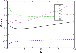
Figure 1: (Color online) Minimum expectation value of $H_{\Omega}$ calculated by a single configuration, $\Phi^{uA}_{KL=0\,M=0}$, Eq. (69), as a function of $K$. The minimum is searched for by varying $\theta,\phi,\zeta$ on the meshes discretized with $M_{\theta}=30$, $M_{\phi}=20$, and $M_{\zeta}=30$ under the constraint that $R_{\rm rms}$ is kept to 1.54 fm. The contributions of $T_{\Omega}$, the nuclear potentials (two-body $V_{\rm 2B}$, and three-body $V_{\rm 3B}$) as well as the Coulomb potential ($V_{\rm C}$) to the minimum energy are also drawn. The curve denoted $H$ is the variation of the total energy.

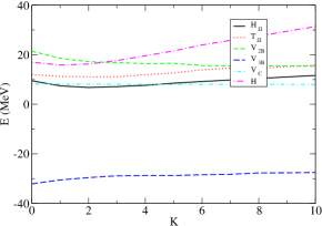
Figure 2: (Color online) The same as Fig. 1 but for $L^{\pi}=2^{+}$.

Table 2: The properties of the single configuration used in Figs. 1 and 2. $\sigma$ is the standard deviation and Overlap is the overlap integral with $K=4$ ($L=0$) or $K=2$ ($L=2$) basis function.

			$L=0$				$L=2$
$K$			$\sigma$	Overlap			$\sigma$	Overlap
0			0.577	0.923			0.477	0.977
1			0.480	0.973			0.431	0.995
2			0.450	0.991			0.400	1.000
3			0.435	0.998			0.374	0.996
4			0.419	1.000			0.378	0.985
5			0.413	0.999			0.381	0.978
6			0.403	0.996			0.373	0.952
7			0.399	0.992			0.365	0.941
8			0.394	0.987			0.338	0.929
9			0.389	0.981			0.338	0.919
10			0.382	0.975			0.332	0.909
11			0.370	0.967
12			0.370	0.962
13			0.358	0.952
14			0.364	0.950
15			0.354	0.940
16			0.356	0.936
17			0.346	0.927
18			0.342	0.919
19			0.334	0.909
20			0.335	0.905

Table 2 lists some properties of the single configuration used in Figs. 1 and 2. It is noted that the standard deviation $\sigma$ decreases as $K$ increases. The configuration with $K=4$ giving the energy minimum for $L=0$ has $\sigma=0.419$. Roughly speaking, this $\sigma$ value corresponds to the degree of localization, $(\sqrt[4]{1+\sigma^{2}}-1)R_{\rm rms}\approx 0.064$ fm around $R_{\rm rms}$. If we want to use more localized configurations, we have to increase $K$. Since the overlap with the $K=4$ configuration decreases very slowly as listed in Overlap column, the energy loss may not be very large. In $L=2$ case, the $K$ dependence of $\sigma$ and the overlap integral appears to decrease faster than the $L=0$ case.

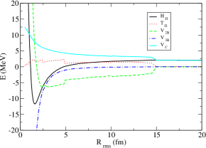
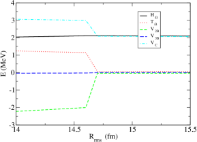
Figure 3: (Color online) (a) Minimum expectation value of $H_{\Omega}$ calculated by a single configuration, $\Phi^{uA}_{K\,L=0\,M=0}$, as a function of $R_{\rm rms}$. The minimum is searched for by varying $K$ as well as $u$ and $A$ that are discretized on the meshes with $M_{\theta}=30$, $M_{\phi}=21$, and $M_{\zeta}=45$. The contributions of $T_{\Omega}$, $V_{\rm 2B}$, $V_{\rm 3B}$, and $V_{\rm C}$ to the minimum energy are also drawn. (b) An enlarged figure of (a) in $R_{\rm rms}=14.0-15.5$ fm.

Figure 3(a) plots the minimum expectation value of $H_{\Omega}$ for $L^{\pi}=0^{+}$ as a function of $R_{\rm rms}$. The minimum energy is obtained by a single configuration determined similarly to the case of Fig. 1, but with slightly finer meshes. We learn how each term of $H_{\Omega}$ responds to the expansion of the system as $R_{\rm rms}$ increases. The $H_{\Omega}$ curve shows a minimum around $R_{\rm rms}$=1.6 fm, and reaches a broad tiny peak at 14.6-14.7 fm, where the contribution of each piece of $H_{\Omega}$ displays a sudden change as magnified in Fig. 3(b). Before the peak, $V_{\rm C}$, $T_{\Omega}$, and $V_{\rm 2B}$ are main contributors to the $H_{\Omega}$ curve, whereas after the peak both contributions of $T_{\Omega}$ and $V_{\rm 2B}$ get small and $V_{\rm C}$ plays a dominant role. Note, however, that the contribution of $V_{\rm 2B}$ persists up to large distances beyond 14 fm, despite the fact that the range of $V_{\alpha\alpha}$ is much shorter than that value. This long-range effect is due to the $\alpha\alpha$ resonance.

Although the minimum expectation value of $H_{\Omega}$ changes smoothly with $R_{\rm rms}$ as seen in Fig. 3(a), the contributions of $T_{\Omega}$ and $V_{\rm 2B}$ show some kinks, especially when $R_{\rm rms}$ changes from 1.6 to 1.7, 2.4 to 2.5, and 4.8 to 4.9 fm. At these points the optimal $K$ value also changes as follows: 4$\to$3, 3$\to$ 2, and 2$\to$1, respectively. However, the minimum expectation value of $H_{\Omega}$ is often not very sensitive to the change of $K$ but several $K$ configurations give almost equal results, whereas the contribution of $T_{\Omega}$ seems to be more sensitive to $K$. This is understood from the degree of localization of the CG. In fact, the $\sigma$ value of $\Phi^{uA}_{KLM}$ decreases with increasing $K$, and hence the contribution of $T_{\Omega}$ tends to increase.

Now we mix various configurations to solve Eq. (18). The constrained equation is solved at the following four points: $R_{\rm rms}$=1.6, 2.5, 5.0, 14.5 fm. The lowest adiabatic channel energy of Ref. suno16 exhibits different character at these points, a steep slope close to the minimum, and a broad plateau close to the three-$\alpha$ threshold. The CG basis functions are generated by including different $K,\theta,\phi$, and $\zeta$ parameters. $K$ is tested up to 20. The mesh points are discretized with $M_{\theta}=30$, $M_{\phi}=21$, and $M_{\zeta}=45$. To avoid possible linear-dependence of the generated basis functions, we exclude any basis function that has overlap of more than 0.95 with other basis functions. We also exclude any configuration whose expectation value of $H_{\Omega}$ is larger than a cut-off energy, $E_{c}$. The value of $E_{c}$ is a bit arbitrary, and it is taken fairly large compared to the expected lowest adiabatic channel energy. The actual basis size is around 250. Note that the basis functions all have $\langle\rho^{2}\rangle=R^{2}$ but they have different $\sigma$ values within $\sigma\leqq 1$.

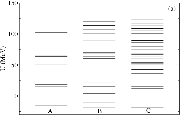
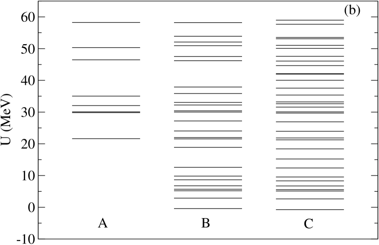
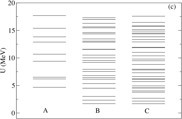
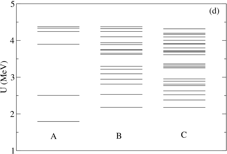
Figure 4: (a) Adiabatic channel energies $U$ at $R_{\rm rms}=1.6$ fm. The basis functions are restricted to have the standard deviation $\sigma\leqq 0.5$ in case A, and $\sigma\leqq 0.75$ in case B, while all the basis functions selected are allowed in case C. See the text for detail. Figures (b), (c), and (d) are the same as (a) but for $R_{\rm rms}=2.5,\,5.0$, and $14.5$ fm, respectively.

In order to see how a spectrum of the adiabatic channel energies changes as the basis size increases, we have tested three calculations: Case A adopts only those basis functions with $\sigma\leqq 0.5$, case B those with $\sigma\leqq 0.75$, and case C is a full basis calculation. In each case we calculate the $\sigma$ value of $\Phi^{JM\pi}_{R\nu}$ and if it is not larger than $\sigma$ that characterizes each case, we accept that $\Phi^{JM\pi}_{R\nu}$ as a solution, otherwise it is discarded. Figure 4 plots the adiabatic channel energies in each case at four $R_{\rm rms}$ radii. The solution of the constrained equations, (18) and (19), appears to be obtained stably. With the increase of the basis size from case A to case C, the density of the adiabatic channel energies considerably increases. Note the different energy scale in Fig. 4(a) to 4(d).

It is interesting to compare the present adiabatic channel energies with those of Ref. suno16 . The latter uses basis functions quite different from ours: At each $\rho$, the channel wave function is expanded in terms of a combination of the product of the Wigner $D$ function and fifth-order basis splines for the two hyperangles. It includes no $\rho$-dependence. In contrast to this, our channel wave function has finite $\rho$-dependence, and therefore receives influence from the adiabatic Hamiltonian at nearby $\rho$ values. Thus both energies need not be necessarily the same but a comparison may indicate characteristics of different types of calculations. Three lowest adiabatic channel energies in MeV obtained in suno16 are $-17.5,\,15.9,\,49.7$ at $R_{\rm rms}=1.6$ fm, $-4.38,\,5.55,\,21.0$ at 2.5 fm, $0.86,\,3.81,\,5.38$ at 5.0 fm, and $0.46,\,0.83,\,1.16$ at 14.5 fm, respectively. Our corresponding energies are $-18.3,\,-16.0\,-11.3$ at 1.6 fm, $-0.75,\,2.63,\,5.12$ at 2.5 fm, $1.68,\,2.16,\,2.68$ at 5.0 fm, and $2.18,\,2.38,\,2.52$ at 14.5 fm. The energy spacing of our calculation is much narrower than that of Ref. suno16 . Which of the two calculations gives lower value for the lowest channel energy seems to depend on $R_{\rm rms}$. At $R_{\rm rms}=2.5$ fm, the calculation of case C actually gives four energies that are lower than $-0.75$ MeV. Since their $\sigma$ values are larger than 1, they are not drawn in Fig. 4(b). Note, however, that the highest one among the four is predicted to be $-4.09$ MeV with $\sigma=1.008$. A calculation with a slightly larger basis set or an optimized basis set would easily predict the lowest adiabatic channel energy around $-4.4$ MeV. The same thing applies to Fig. 4(d). The lowest energy of case C is higher than that of case A. A few solutions of case C are, however, lower than the lowest adiabatic channel energy of case A, but they are not shown because their $\sigma$ values are larger than 1. One of them is located at 1.79 MeV and has $\sigma=1.08$. It is still considerably higher than the lowest energy, $0.46$ MeV, of Ref. suno16 .

V Summary

We have formulated hyperspherical calculations using the flexibility of the correlated Gaussians. Differently from conventional hyperspherical methods, the channel wave function and the adiabatic channel energy are defined by solving the hyperradius-constrained eigenvalue equation of the adiabatic Hamiltonian. This approach enables us to perform standard configuration interaction calculations.

This work takes a non-conventional venue by allowing the spread of the value of the hyperradius for a given basis function. While in previous hyperspherical calculations, e.g. in suno16 , the basis functions belong to a given hyperradius, in the present work “the basis functions are localized”, that is, the hyperradii of the basis functions reside in a narrow region around a predefined hyperradius. This approach has its advantages and disadvantages. A slight disadvantage is that one can not define a sharp hyperradius, so that the direct comparison to conventional calculations is not simple, whereas an advantage is that the basis functions directly couple the neighboring regions which may help to resolve complicated dynamical processes. A further advantage is the easier access to larger systems.

The present formulation is expected to have many applications. As an example, we just mention one problem, the fragmentation or decay of a nucleus into several $\alpha$ particles at large distances, as discussed in girod13 ; royer15 ; royer14 . The approaches employed there have limitations in taking into account important effects such as couplings with other configurations, the angular momentum dependence of the adiabatic potential, and the removal of spurious center-of-mass excitations. Since the issue is exactly concerned with how the system evolves as it expands, it is worthwhile attempting at resolving those problems in the hyperspherical approach.

Appendix A Solving a constrained eigenvalue problem

The aim of this appendix is to solve a problem of obtaining the eigenvalues and corresponding eigenfunctions of a Hermitian operator $H$ with a constraint. It is formulated as follows: Let $Q$ be a positive-definite Hermitian operator, and let ($\phi_{1},\phi_{2},\ldots,\phi_{n}$) be a given set of normalized, independent basis functions. Obtain, in the space spanned by the set, as many $\Phi$’s possible that make the expectation value of $H$

$$\frac{\langle\Phi|H|\Phi\rangle}{\langle\Phi|\Phi\rangle}$$ (78)

stationary under the constraint

$$\frac{\langle\Phi|Q|\Phi\rangle}{\langle\Phi|\Phi\rangle}=q,$$ (79)

where $q$ is a positive constant. The condition $\langle\phi_{i}|Q|\phi_{i}\rangle=q$ is assumed for each $\phi_{i}$ in the text. It may not be absolutely necessary, however, although the number of solutions may depend on how many basis functions satisfy the condition.

This type of problem appears in several cases. See, for example, Ref. flocard73 for the optimization of $\Phi$ and Ref. kukulin78 for the determination of $\Phi$ free from some configurations. The present problem has distinct differences from those cases in that the available configuration space is preset and several solutions are requested if possible.

We construct an orthonormal set, $(\psi_{1},\psi_{2},\ldots,\psi_{n})$, that makes $Q$ diagonal. To do this, we first diagonalize the overlap matrix $(\langle\phi_{i}|\phi_{j}\rangle)$:

$$\sum_{j=1}^{n}\langle\phi_{i}|\phi_{j}\rangle u^{(k)}_{j}=b_{k}u^{(k)}_{i},$$ (80)

where $\sum_{i=1}^{n}u^{(k)}_{i}u^{(l)}_{i}=\delta_{kl}$. The basis set $u_{k}$ defined by

$$u_{k}=\frac{1}{\sqrt{b_{k}}}\sum_{i=1}^{n}u^{(k)}_{i}\phi_{i}\ \ \ (k=1,\ldots,n)$$ (81)

is orthonormal, $\langle u_{k}|u_{l}\rangle=\delta_{kl}$. Next, diagonalizing $Q$ in the set $u_{k}$,

$$\sum_{j=1}^{n}\langle u_{i}|Q|u_{j}\rangle\psi^{(k)}_{j}=q_{k}\psi^{(k)}_{i},$$ (82)

with $\sum_{i=1}^{n}\psi^{(k)}_{i}\psi^{(l)}_{i}=\delta_{kl}$, we construct the set $\psi_{k}$ as

$$\psi_{k}=\sum_{i=1}^{n}\psi^{(k)}_{i}u_{i},$$ (83)

which has the desired property, $\langle\psi_{k}|\psi_{l}\rangle=\delta_{kl}$, and $\langle\psi_{k}|Q|\psi_{l}\rangle=q_{k}\delta_{kl}$. It is easy to express $\psi_{i}$ in terms of the original set $\phi_{i}$’s.

We attempt to obtain $\Phi$’s step by step. Defining a Hermitian operator $H^{\prime}$ with a Lagrange multiplier $\lambda$,

$$H^{\prime}(\lambda)=H-\lambda(Q-q),$$ (84)

we solve the eigenvalue problem,

$$H^{\prime}(\lambda)\Phi(\lambda)=E^{\prime}(\lambda)\Phi(\lambda),$$ (85)

using the set $\psi_{i}$, and calculate the expectation value,

$$F(\lambda) =\langle\Phi(\lambda)|Q-q|\Phi(\lambda)\rangle$$

$$=\langle\Phi(\lambda)|Q|\Phi(\lambda)\rangle-q,$$ (86)

where $\Phi(\lambda)$ is normalized. Focusing always on the lowest-energy solution for any $\lambda$, we vary $\lambda$ to find a zero of $F(\lambda)$: $F(\lambda_{1})=0$. Then $\Phi(\lambda_{1})$ satisfies the constraint (79) and that is the solution to be found: $\Phi_{1}=\Phi(\lambda_{1})$ with the energy $E_{1}=E^{\prime}(\lambda_{1})$.

To determine the next solution, we define a configuration space of dimension $(n-1)$ by removing $\Phi_{1}$ from the set $(\psi_{1},\psi_{2},\ldots,\psi_{n})$, and follow the above procedure to find a successful solution $\Phi_{2}$. This process continues until no new solution is found. Clearly $\Phi_{i}$’s determined in this way are orthogonal to each other.

We can show that $\Phi_{i}$ and $\Phi_{j}$ for $i\neq j$ have no coupling matrix element of $H$ if $\lambda_{i}\neq\lambda_{j}$. Since both functions are orthogonal, the matrix element of $H$ reduces to that of $Q$ as follows:

$$\langle\Phi_{j}|H|\Phi_{i}\rangle =\langle\Phi_{j}|H^{\prime}(\lambda_{i})+\lambda_{i}(Q-q)|\Phi_{i}\rangle$$

$$=E^{\prime}(\lambda_{i})\langle\Phi_{j}|\Phi_{i}\rangle+\lambda_{i}\langle\Phi_{j}|Q-q|\Phi_{i}\rangle$$

$$=\lambda_{i}\langle\Phi_{j}|Q|\Phi_{i}\rangle.$$ (87)

Because of $\langle\Phi_{j}|H|\Phi_{i}\rangle=\langle\Phi_{i}|H|\Phi_{j}\rangle^{*}=\lambda_{j}\langle\Phi_{i}|Q|\Phi_{j}\rangle^{*}=\lambda_{j}\langle\Phi_{j}|Q|\Phi_{i}\rangle$, it follows that

$$(\lambda_{i}-\lambda_{j})\langle\Phi_{j}|Q|\Phi_{i}\rangle=0.$$ (88)

If $\lambda_{i}\neq\lambda_{j}$, $\langle\Phi_{j}|Q|\Phi_{i}\rangle$ vanishes and consequently $\langle\Phi_{j}|H|\Phi_{i}\rangle$ must vanish.

If $\lambda_{i}$ and $\lambda_{j}$ are accidentally equal, the above argument does not apply and it is not clear whether or not $H$ has the coupling matrix element.

Appendix B Examples of correlated-Gaussian matrix element

We show the examples of Eq. (30) that appear frequently. For ${\cal O}(\bm{x})$, let us consider the following terms:

$${\rm(i)}\ \ \ \ {\widetilde{\bm{w}}}\bm{x},$$

$${\rm(ii)}\ \ \ ({\widetilde{\bm{w}}}\bm{x})({\widetilde{{\bm{w}}^{\prime}}}\bm{x}),$$

$${\rm(iii)}\ \ \ {\widetilde{\bm{x}}}C\bm{x},$$

$${\rm(iv)}\ \ \ ({\widetilde{\bm{w}}}\bm{x})({\widetilde{\bm{x}}}C\bm{x}),$$

$${\rm(v)}\ \ \ \ ({\widetilde{\bm{x}}}C\bm{x})({\widetilde{\bm{x}}}C^{\prime}\bm{x}).$$ (89)

Here $\bm{w}$ and ${\bm{w}}^{\prime}$ are column vectors of dimension $(N-1)$ whose elements are 3-dimensional vectors, and $C$ and $C^{\prime}$ are $(N-1)\times(N-1)$ symmetric matrices, and they are all independent of $\bm{x}$. The integral of Eq. (30) is easily obtained. Corresponding to (i)-(v) classes, ${\cal P_{O}}$ reads

$${\rm(i)}\ \ \ \frac{1}{2}\widetilde{\bm{w}}B^{-1}\bm{v},$$

$${\rm(ii)}\ \ \ \frac{1}{2}\widetilde{\bm{w}}B^{-1}{\bm{w}}^{\prime}+\frac{1}{4}\widetilde{\bm{w}}B^{-1}\bm{v}\,\widetilde{{\bm{w}}^{\prime}}B^{-1}\bm{v},$$

$${\rm(iii)}\ \ \ \frac{3}{2}{\rm Tr}B^{-1}C+\frac{1}{4}\widetilde{\bm{v}}B^{-1}CB^{-1}\bm{v},$$

$${\rm(iv)}\ \ \ \frac{1}{2}\widetilde{\bm{w}}B^{-1}CB^{-1}\bm{v}+\frac{3}{4}(\widetilde{\bm{w}}B^{-1}\bm{v})\,{\rm Tr}B^{-1}C$$

$$\qquad\ \ +\frac{1}{8}(\widetilde{\bm{w}}B^{-1}\bm{v})(\widetilde{\bm{v}}B^{-1}CB^{-1}\bm{v}),$$

$${\rm(v)}\ \ \ \frac{3}{2}{\rm Tr}B^{-1}CB^{-1}C^{\prime}+\frac{1}{2}\widetilde{\bm{v}}B^{-1}CB^{-1}C^{\prime}B^{-1}\bm{v}$$

$$\qquad\ \ +\Big{(}\frac{3}{2}{\rm Tr}B^{-1}C+\frac{1}{4}\widetilde{\bm{v}}B^{-1}CB^{-1}\bm{v}\Big{)}$$

$$\qquad\ \ \times\Big{(}\frac{3}{2}{\rm Tr}B^{-1}C^{\prime}+\frac{1}{4}\widetilde{\bm{v}}B^{-1}C^{\prime}B^{-1}\bm{v}\Big{)}.$$ (90)

As an example, we show how to obtain the matrix element of $\widetilde{\bm{x}}C\bm{x}$ belonging to class (iii). The corresponding ${\cal P_{O}}$ reads

$$\frac{3}{2}{\rm Tr}B^{-1}C+\frac{1}{4}\widetilde{\bm{v}}G_{1}\bm{v}$$ (91)

with $G_{1}=B^{-1}CB^{-1}$, and it comprises four terms:

$$T_{000}=\frac{3}{2}{\rm Tr}B^{-1}C,\ \ \ T_{100}=\frac{1}{4}\widetilde{u}G_{1}u,$$

$$T_{010}=\frac{1}{4}\widetilde{u^{\prime}}G_{1}u^{\prime},\ \ \ T_{001}=\frac{1}{2}\widetilde{u}G_{1}u^{\prime},$$ (92)

where $T_{kk^{\prime}l}$ is an abbreviation of $T_{kk^{\prime}l}(u^{\prime}A^{\prime},uA)$. Equation (48) immediately gives us the following result:

$$\langle f^{u^{\prime}A^{\prime}}_{K^{\prime}LM}|\widetilde{\bm{x}}C\bm{x}|f^{uA}_{KLM}\rangle$$

$$=\langle f^{u^{\prime}A^{\prime}}_{K^{\prime}LM}|f^{uA}_{KLM}\rangle\Big{[}\ \frac{3}{2}{\rm Tr}B^{-1}C+\frac{\widetilde{u}G_{1}u}{\widetilde{u}B^{-1}u}F^{KK^{\prime}L}_{100}(z)$$

$$\ \ +\frac{\widetilde{u^{\prime}}G_{1}u^{\prime}}{\widetilde{u^{\prime}}B^{-1}u^{\prime}}F^{KK^{\prime}L}_{010}(z)+\frac{\widetilde{u}G_{1}u^{\prime}}{\widetilde{u}B^{-1}u^{\prime}}F^{KK^{\prime}L}_{001}(z)\Big{]}.$$ (93)

The matrix element of $(\widetilde{\bm{x}}C\bm{x})^{2}$ is obtained similarly:

$$\langle f^{u^{\prime}A^{\prime}}_{K^{\prime}LM}|(\widetilde{\bm{x}}C\bm{x})^{2}|f^{uA}_{KLM}\rangle=\langle f^{u^{\prime}A^{\prime}}_{K^{\prime}LM}|f^{uA}_{KLM}\rangle\Big{[}\,\frac{3}{2}{\rm Tr}G_{1}C+\frac{9}{4}({\rm Tr}B^{-1}C)^{2}+(2\widetilde{u}G_{2}u+3{\rm Tr}B^{-1}C\widetilde{u}G_{1}u)\frac{1}{\widetilde{u}B^{-1}u}F^{KK^{\prime}L}_{100}(z)$$

$$+(2\widetilde{u^{\prime}}G_{2}u^{\prime}+3{\rm Tr}B^{-1}C\widetilde{u^{\prime}}G_{1}u^{\prime})\frac{1}{\widetilde{u^{\prime}}B^{-1}u^{\prime}}F^{KK^{\prime}L}_{010}(z)+(2\widetilde{u}G_{2}u^{\prime}+3{\rm Tr}B^{-1}C\widetilde{u}G_{1}u^{\prime})\frac{1}{\widetilde{u}B^{-1}u^{\prime}}F^{KK^{\prime}L}_{001}(z)$$

$$+\frac{(\widetilde{u}G_{1}u)^{2}}{(\widetilde{u}B^{-1}u)^{2}}F^{KK^{\prime}L}_{200}(z)+\frac{(\widetilde{u^{\prime}}G_{1}u^{\prime})^{2}}{(\widetilde{u^{\prime}}B^{-1}u^{\prime})^{2}}F^{KK^{\prime}L}_{020}(z)+\frac{(\widetilde{u}G_{1}u^{\prime})^{2}}{(\widetilde{u}B^{-1}u^{\prime})^{2}}F^{KK^{\prime}L}_{002}(z)$$

$$+2\frac{(\widetilde{u}G_{1}u)(\widetilde{u^{\prime}}G_{1}u^{\prime})}{(\widetilde{u}B^{-1}u)(\widetilde{u^{\prime}}B^{-1}u^{\prime})}F^{KK^{\prime}L}_{110}(z)+2\frac{(\widetilde{u}G_{1}u)(\widetilde{u}G_{1}u^{\prime})}{(\widetilde{u}B^{-1}u)(\widetilde{u}B^{-1}u^{\prime})}F^{KK^{\prime}L}_{101}(z)+2\frac{(\widetilde{u^{\prime}}G_{1}u^{\prime})(\widetilde{u^{\prime}}G_{1}u)}{(\widetilde{u^{\prime}}B^{-1}u^{\prime})(\widetilde{u^{\prime}}B^{-1}u)}F^{KK^{\prime}L}_{011}(z)\Big{]},$$ (94)

where $G_{2}=B^{-1}CB^{-1}CB^{-1}$.

References

- (1) M. V. Zhukov, B. V. Danilin, D. V. Fedorov, J. M. Bang, I. J. Thompson, and J. S. Vaagen, Phys. Rep. 231, 151 (1993).
- (2) C. D. Lin, Phys. Rep. 257, 1 (1995).
- (3) R. Krivec, Few-Body Syst. 25, 199 (1998).
- (4) E. Nielsen, D. V. Fedorov, A. S. Jensen, and E. Garrido, Phys. Rep. 347, 373 (2001).
- (5) C. H. Greene, P. Giannakeas, and J. Pérez-Ríos, Rev. Mod. Phys. 89, 035006 (2017).
- (6) I. J. Thompson, B. V. Danilin, V. D. Efros, J. S. Vaagen, J. M. Bang, and M. V. Zhukov, Phys. Rev. C 61, 024318 (2000).
- (7) J. Macek, J. Phys. B 1, 831 (1968).
- (8) A. A. Kvitsinsky and V. V. Kostrykin, J. Math. Phys. 32, 2802 (1991).
- (9) N. B. Nguyen, F. M. Nunes, and I. J. Thompson, Phys. Rev. C 87, 054615 (2013).
- (10) S. Ishikawa, Phys. Rev. C 87, 055804 (2013).
- (11) H. Suno, Y. Suzuki, and P. Descouvemont, Phys. Rev. C 94, 054607 (2016).
- (12) H. Suno, Y. Suzuki, and P. Descouvemont, Phys. Rev. C 91, 014004 (2015).
- (13) N. Barnea, W. Leidemann, and G. Orlandini, Phys. Rev. C 61, 054001 (2000).
- (14) N. Barnea, W. Leidemann, and G. Orlandini, Phys. Rev. C 67, 054003 (2003).
- (15) N. Barnea, W. Leidemann, and G. Orlandini, Phys. Rev. C 81, 064001 (2010).
- (16) S. Bacca, N. Barnea, and A. Schwenk, Phys. Rev. C 86, 034321 (2012).
- (17) N. K. Timofeyuk, Phys. Rev. C 65, 064306 (2002).
- (18) N. K. Timofeyuk, Phys. Rev. C 78, 054314 (2008).
- (19) M. Gattobigio, A. Kievsky, and M. Viviani, Phys. Rev. C 83, 024001 (2011).
- (20) J. von Stecher and C. H. Greene, Phys. Rev. A 80, 022504 (2009).
- (21) S. T. Rittenhouse, J. von Stecher, J. P. D’Incao, N. P. Mehta, and C. H. Greene, J. Phys. B: At. Mol. Opt. Phys. 44, 172001 (2011).
- (22) D. Rakshit and D. Blume, Phys. Rev. A 86, 062513 (2012).
- (23) K. M. Daily and C. H. Greene, Phys. Rev. A 89, 012503 (2014).
- (24) S. F. Boys, Proc. R. Soc. London, Ser. A 258, 402 (1960).
- (25) K. Singer, Proc. R. Soc. London, Ser. A 258, 412 (1960).
- (26) K. Varga and Y. Suzuki, Phys. Rev. C 52, 2885 (1995).
- (27) Y. Suzuki and K. Varga, Stochastic Variational Approach to Quantum-Mechanical Few-Body Problems, Lecture Notes in Physics, m 54, (Springer, Berlin, 1998).
- (28) Y. Suzuki, J. Usukura and K. Varga, J. Phys. B: At. Mol. Opt. Phys. 31, 31 (1998).
- (29) K. Varga, Y. Suzuki, and R. G. Lovas, Nucl. Phys. A 571, 447 (1994).
- (30) J. Mitroy, S. Bubin, W. Horiuchi, Y. Suzuki, L. Adamowicz, W. Cencek, K. Szalewicz, J. Komasa, D. Blume, and K. Varga, Rev. Mod. Phys. 85, 693 (2013).
- (31) W. Horiuchi and Y. Suzuki, Phys. Rev. C 89, 011304 (2014).
- (32) D. Mikami, W. Horiuchi, and Y. Suzuki, Phys. Rev. C 89, 064302 (2014).
- (33) Y. Suzuki, Prog. Theor. Exp. Phys. 2015, 043D05.
- (34) O. I. Tolstikhin, S. Watanabe, and M. Matsuzawa, J. Phys. B: At. Mol. Opt. Phys. 29, L 389, (1996).
- (35) H. Suno, J. Chem. Phys. 134, 064318 (2011).
- (36) Y. Suzuki, W. Horiuchi, M. Orabi and K. Arai, Few-Body Syst. 42, 33 (2008).
- (37) S. Aoyama, K. Arai, Y. Suzuki, P. Descouvemont, and D. Baye, Few-Body Syst. 52, 97 (2012).
- (38) Y. Suzuki and W. Horiuchi, Phys. Rev. C 95, 044320 (2017).
- (39) A. Erdélyi, W. Magnus, F. Oberhettinger, and F. G. Tricomi, Higher Transcendental Functions, Vol. I, (MacGraw-Hill, New York, 1953).
- (40) M. Abramowitz and I. A. Stegun, Handbook of Mathmatical Functions with Formulas, Graphs, and Mathematical Tables (Dover, Mineola, New York, 1970).
- (41) Y. Suzuki and M. Takahashi, Phys. Rev. C 65, 064318 (2002).
- (42) S. Ali and A. R. Bodmer, Nucl. Phys. 80, 99 (1966).
- (43) M. Girod and P. Schuck, Phys. Rev. Lett. 111, 132503 (2013).
- (44) G. Royer, G. Rmasamy, and P. Eudes, Phys. Rev. C 92, 054308 (2015).
- (45) G. Royer, A. Escudie, and B. Sublard, Phys. Rev. C 90, 024607 (2014).
- (46) H. Flocard, P. Quentin, A. K. Kerman, and D. Vautherin, Nucl. Phys. A 203, 433 (1973).
- (47) V. I. Kukulin and V. N. Pomerantsev, Ann. Phys. 111, (1978) 330.