Abstract

Large models are prevalent in modern machine learning scenarios, including deep learning, recommender systems, etc., which can have millions or even billions of parameters. Parallel algorithms have become an essential solution technique to many large-scale machine learning jobs. In this paper, we propose a model parallel proximal stochastic gradient algorithm, AsyB-ProxSGD, to deal with large models using model parallel blockwise updates while in the meantime handling a large amount of training data using proximal stochastic gradient descent (ProxSGD). In our algorithm, worker nodes communicate with the parameter servers asynchronously, and each worker performs proximal stochastic gradient for only one block of model parameters during each iteration. Our proposed algorithm generalizes ProxSGD to the asynchronous and model parallel setting. We prove that AsyB-ProxSGD achieves a convergence rate of $O(1/\sqrt{K})$ to stationary points for nonconvex problems under constant minibatch sizes, where $K$ is the total number of block updates. This rate matches the best-known rates of convergence for a wide range of gradient-like algorithms. Furthermore, we show that when the number of workers is bounded by $O(K^{1/4})$, we can expect AsyB-ProxSGD to achieve linear speedup as the number of workers increases. We implement the proposed algorithm on MXNet and demonstrate its convergence behavior and near-linear speedup on a real-world dataset involving both a large model size and large amounts of data.

1 Introduction

Many machine learning problems can be formulated as the following general minimization framework:

$$\begin{split}\mathop{\min}_{x\in d}&\quad\Psi(x):=\frac{1}{n}\sum_{i=1}^{n}f_{i}(x)+h(x),\end{split}$$ (1)

where $f_{i}(x)$ is typically a smooth yet possibly nonconvex loss function of the $i$-th sample, and $h(x)$ is a convex yet nonsmooth regularizer term that promotes some structures. Examples include deep learning with regularization Dean et al. (2012); Chen et al. (2015); Zhang et al. (2015), LASSO Tibshirani et al. (2005), sparse logistic regression Liu et al. (2009), robust matrix completion Xu et al. (2010); Sun and Luo (2015), and sparse support vector machine (SVM) Friedman et al. (2001).

Many classical deterministic (non-stochastic) algorithms are available to solve problem (1), including the proximal gradient (ProxGD) method Parikh et al. (2014) and its accelerated variants Li and Lin (2015) as well as the alternating direction method of multipliers (ADMM) Hong et al. (2016). These methods leverage the so-called proximal operators Parikh et al. (2014) to handle the nonsmoothness in the problem. However, these algorithms require calculating the gradient of all $n$ samples in each iteration, which is expensive in modern machine learning problems. The trend to deal with large volumes of data is the use of stochastic algorithms. As the number of training samples $n$ increases, the cost of updating the model $x$ taking into account all error gradients becomes prohibitive. To tackle this issue, stochastic algorithms make it possible to update $x$ using only a small subset of all training samples at a time.

Stochastic gradient descent (SGD) is one of the first algorithms widely implemented in an asynchronous parallel fashion; its convergence rates and speedup properties have been analyzed for both convex Agarwal and Duchi (2011); Mania et al. (2017) and nonconvex Lian et al. (2015) optimization problems. Nevertheless, SGD is mainly applicable to the case of smooth optimization, and yet is not suitable for problems with a nonsmooth term in the objective function, e.g., an $\ell_{1}$ norm regularizer. In fact, such nonsmooth regularizers are commonplace in many practical machine learning problems or constrained optimization problems. In these cases, SGD becomes ineffective, as it is hard to obtain gradients for a nonsmooth objective function.

With rapidly growing data volumes and model complexity, the need to scale up machine learning has sparked broad interests in developing efficient parallel optimization algorithms. A typical parallel optimization algorithm usually decomposes the original problem into multiple subproblems, each handled by a worker node. Each worker iteratively downloads the global model parameters and computes its local gradients to be sent to the master node or servers for model updates. Recently, asynchronous parallel optimization algorithms Niu et al. (2011); Li et al. (2014b); Lian et al. (2015), exemplified by the Parameter Server architecture Li et al. (2014a), have been widely deployed in industry to solve practical large-scale machine learning problems. Asynchronous algorithms can largely reduce overhead and speedup training, since each worker may individually perform model updates in the system without synchronization.

Existing parallel algorithms fall into two categories: data parallelism and model parallelism. In data parallelism, each worker takes a subset of training samples $i$ and calculates their loss functions $f_{i}$’s and/or gradients in parallel. For example, a typical implementation of parallel SGD is to divide a minibatch with $N$ samples into several smaller minibatches (each with $N^{\prime}$ samples), and each worker computes gradients on $N^{\prime}$ samples. This is preferred when the size of data $n$ is large. In model parallelism, the model parameters $x$ is partitioned into $M$ blocks, where $x_{j}\in d_{j}$ with $d_{j}\in\mathbb{N}_{+}$ and $\sum_{j=1}^{M}d_{j}=d$. Since proximal operator on $x$ can be decomposed into those on individual blocks Parikh et al. (2014), proximal gradient and its stochastic version (proximal stochastic gradient descent or ProxSGD) is again a natural candidate to solve (1). Zhou et al. (2016) shows that Block Proximal Gradient Descent works in an asynchronous parallel mode, and in the meantime proves that Block ProxSGD can converge to critical points when the maximum staleness is bounded. However, theoretical understanding of the behavior of Asynchronous Block ProxSGD, a more useful algorithm in practical Parameter Servers, is a gap yet to be filled.

In this paper, we propose AsyB-ProxSGD (Asynchronous Block Proximal Stochastic Gradient Descent), an extension of proximal stochastic gradient (ProxSGD) algorithm to the model parallel paradigm and to the partially asynchronous protocol (PAP) setting. In AsyB-ProxSGD, workers asynchronously communicate with the parameter servers, which collectively store model parameters in blocks. In an iteration, each worker pulls the latest yet possibly outdated model from servers, calculates partial gradients for only one block based on stochastic samples, and pushes the gradients to the corresponding server. As workers can update different blocks in parallel, AsyB-ProxSGD is different from traditional data parallel ProxSGD can handle both a large model size $d$ and a large number $n$ of training samples, a case frequently observed in reality.

Our theoretical contribution is summarized as follows. We prove that AsyB-ProxSGD can converge to stationary points of the nonconvex and nonsmooth problem (1) with an ergodic convergence rate of $O(1/\sqrt{K})$, where $K$ is the total number of times that any block in $x$ is updated. This rate matches the convergence rate known for asynchronous SGD. The latter, however, is suitable only for smooth problems. To our best knowledge, this is the first work that provides convergence rate guarantees for ProxSGD in a model parallel mode, especially in an asynchronous setting. We also provide a linear speedup guarantee as the number of workers increases, provided that the number of workers is bounded by $O({K}^{1/4})$. This result has laid down a theoretical ground for the scalability and performance of AsyB-ProxSGD in practice. Evaluation based on a real-world dataset involving both a large model and a large dataset has corroborated our theoretical findings on the convergence and speedup behavior of AsyB-ProxSGD, under a Parameter Server implementation.

2 Preliminaries

In this section, we first introduce some notations to be used throughout the paper. Then we introduce the stochastic optimization problem to be studied. Finally, we introduce proximal operators and enumerate fundamental assumptions made in the model.

We use $\lVert{x}\rVert$ to denote the $\ell_{2}$ norm of the vector $x$, and $\langle{x,y}\rangle$ to denote the inner product of two vectors $x$ and $y$. We use $g(x)$ to denote the “true” gradient $\nabla f(x)$ and use $G(x;\xi)$ to denote the stochastic gradient $\nabla F(x;\xi)$ for a function $f(x)$. Let $\nabla_{j}$ be the derivative w.r.t. $x_{j}$, the $j$-th coordinate of $x$; and let $G_{j}$ and $g_{j}$ represent $\nabla_{j}F(x;\xi)$ and $\nabla_{j}f(x)$, respectively. For a random variable or vector $X$, let $\mathbb{E}[X|\mathcal{F}]$ be the conditional expectation of $X$ w.r.t. a sigma algebra $\mathcal{F}$.

2.1 Stochastic Optimization Problems

In this paper, we consider the following stochastic optimization problem instead of the original deterministic version (1):

$$\begin{split}\mathop{\min}_{x\in d}&\quad\Psi(x):=\mathbb{E}_{\xi}[F(x;\xi)]+h(x),\end{split}$$ (2)

where the stochastic nature comes from the random variable $\xi$, which in our problem settings, represents a random index selected from the training set $\{1,\ldots,n\}$. Therefore, (2) attempts to minimize the expected loss of a training sample plus a regularizer $h(x)$. When it comes to large models, we decompose $x$ into $M$ blocks, and rewrite (2) into the following block optimization form:

$$\mathop{\min}_{x\in d}\Psi(x):=\mathbb{E}_{\xi}[F(x_{1},\ldots,x_{M};\xi)]+\sum_{j=1}^{M}h_{j}(x_{j}),$$ (3)

where $x=(x_{1},\ldots,x_{M})$, $x_{j}\in d_{j}$ for those $d_{j}\in\mathbb{N}_{+}$ and $\sum_{j=1}^{M}d_{j}=d$, and $h(x)=\sum_{j=1}^{M}h_{j}(x_{j})$.

In this work, we assume all $h_{j}$’s for problem (3) are proper, closed and convex, yet not necessarily smooth. To handle the potential non-smoothness, we introduce the following generalized notion of derivatives to be used in convergence analysis.

Definition 1 (Subdifferential e.g., Parikh et al. (2014)).

We say a vector $p\in d$ is a subgradient of the function $h:d\to$ at $x\in\mathrm{dom}\ h$, if for all $z\in\mathrm{dom}\ h$,

$$h(z)\geq h(x)+\langle{p,z-x}\rangle.$$ (4)

Moreover, denote the set of all such subgradients at $x$ by $\partial h(x)$, which is called the subdifferential of $h$ at $x$.

For problems (2) and  (3), we define the critical point as follows:

Definition 2 (Critical point Attouch et al. (2013)).

A point $x\in d$ is a critical point of $\Psi$, iff $0\in\nabla f(x)+\partial h(x)$.

2.2 Proximal Gradient Descent

The proximal operator is fundamental to many algorithms to solve problem (1) as well as its stochastic variants (2) and (3).

Definition 3 (Proximal operator).

The proximal operator $\mathbf{prox}$ of a point $x\in d$ under a proper and closed function $h$ with parameter $\eta>0$ is defined as:

$$\mathbf{prox}_{\eta h}(x)=\mathop{\arg\min}_{y\in d}\left\{h(y)+\frac{1}{2\eta}\lVert{y-x}\rVert^{2}\right\}.$$ (5)

In its vanilla version, proximal gradient descent performs the following iterative updates:

$$x^{k+1}\leftarrow\mathbf{prox}_{\eta_{k}h}(x^{k}-\eta_{k}\nabla f(x^{k})),$$

for $k=1,2,\ldots$, where $\eta_{k}>0$ is the step size at iteration $k$.

To solve stochastic optimization problems (2) and (3), we need a variant called proximal stochastic gradient descent (ProxSGD), with its update rule at iteration $k$ given by

$$x^{k+1}\leftarrow\mathbf{prox}_{\eta_{k}h}\left(x^{k}-\frac{\eta_{k}}{\lvert\Xi_{k}\rvert}\sum_{\xi\in\Xi_{k}}\nabla F(x^{k};\xi)\right).$$

In ProxSGD, the gradient $\nabla f$ is replaced by the gradients from a random subset of training samples, denoted by $\Xi_{k}$ at iteration $k$. Since $\xi$ is a random variable indicating a random index in $\{1,\ldots,n\}$, $F(x;\xi)$ is a random loss function for the random sample $\xi$, such that $f(x):=\mathbb{E}_{\xi}[F(x;\xi)]$.

With these definitions, we now introduce our metric used in ergodic convergence analysis:

$$P(x,g,\eta):=\frac{1}{\eta}(x-\mathbf{prox}_{\eta h}(x-\eta g)),$$

which is also called the gradient mapping in the literature, e.g., Parikh et al. (2014). For non-convex problems, it is a standard approach to measure convergence (to a stationary point) by gradient mapping according to the following lemma:

Lemma 1 (Non-convex Convergence Attouch et al. (2013)).

A point $x$ is a critical point of (2) iff. $P(x,g,\eta)=0$.

Therefore, we can use the following definition as a convergence metric:

Definition 4 (Iteration complexity Reddi et al. (2016)).

A solution $x$ is called $\epsilon$-accurate, if $\mathbb{E}[\lVert{P(x,g,\eta)}\rVert^{2}]\leq\epsilon$ for some $\eta>0$. If an algorithm needs at least $K$ iterations to find an $\epsilon$-accurate solution, its iteration complexity is $K$.

We make the following assumptions throughout the paper. Other algorithm specific assumptions will be introduced later in the corresponding sections.

We assume that $f(\cdot)$ is a smooth function with the following properties:

Assumption 1 (Lipschitz Gradient).

For function $f$ there are Lipschitz constants $L_{j},L>0$ such that

$$\lVert{\nabla f(x)-\nabla f(y)}\rVert\leq L\lVert{x-y}\rVert,\forall x,y\in d,$$ (6)

$$\lVert{\nabla_{j}f(x)-\nabla_{j}f(x+\alpha e_{j})}\rVert\leq L_{\max}|\alpha|,\forall x\in d,$$ (7)

where $e_{j}$ is an indicator vector that is only valid at block $j$ with value 1, and vanishes to zero at other blocks. Clearly we have $L_{\max}\leq L$.

As discussed above, assume that $h$ (or $h_{j}$) is a proper, closed and convex function, which is yet not necessarily smooth. If the algorithm has been executed for $k$ iterations, we let $\mathcal{F}_{k}$ denote the set that consists of all the samples used up to iteration $k$. Since $\mathcal{F}_{k}\subseteq\mathcal{F}_{k^{\prime}}$ for all $k\leq k^{\prime}$, the collection of all such $\mathcal{F}_{k}$ forms a filtration. Under such settings, we can restrict our attention to those stochastic gradients with an unbiased estimate and bounded variance, which are common in the analysis of stochastic gradient descent or stochastic proximal gradient algorithms, e.g., Lian et al. (2015); Ghadimi et al. (2016).

Assumption 2 (Unbiased gradient).

For any $k$, we have $\mathbb{E}[G_{k}|\mathcal{F}_{k}]=g_{k}$.

Assumption 3 (Bounded variance).

The variance of the stochastic gradient is bounded by $\mathbb{E}[\lVert{G(x;\xi)-\nabla f(x)}\rVert^{2}]\leq\sigma^{2}$.

2.3 Parallel Stochastic Optimization

Recent years have witnessed rapid development of parallel and distributed computation frameworks for large-scale machine learning problems. One popular architecture is called parameter server Dean et al. (2012); Li et al. (2014a), which consists of some worker nodes and server nodes. In this architecture, one or multiple master machines play the role of parameter servers, which maintain the model $x$. All other machines are worker nodes that communicate with servers for training machine learning models. In particular, each worker has two types of requests: pull the current model $x$ from servers, and push the computed gradients to servers.

Before proposing our AsyB-ProxSGD algorithm in the next section, let us first introduce its synchronous version. Suppose we execute ProxSGD with a minibatch of 128 random samples on 8 workers and our goal is to use these 8 workers to train a model with 8 blocks. We can let each worker randomly take 128 samples, compute a summed partial gradient w.r.t one block (say, block $j$) on them, and push it to server $j$. In synchronous case, server $j$ will finally receive 8 summed partial gradients on 8 blocks (each partial gradient contains information of 128 samples) in each iteration. This server then updates the model by performing the proximal gradient descent step. In general, if we divide the model into $M$ blocks, each worker will be assigned to update only one block using a minibatch of $N$ samples and they can do updating in parallel in an iteration.

Note that in this scenario, all workers have to calculate the whole minibatch of the computation. Thanks to the decomposition property of proximal operator Parikh et al. (2014), updating blocks can be done in parallel by servers, which corresponds to model parallelism in the literature (e.g., Niu et al. (2011); Zhou et al. (2016); Pan et al. (2016)). Another type of parallelism is called data parallelism, in which each worker uses only part of $N$ random samples in the minibatch to compute a full gradient on $x$ (e.g., Agarwal and Duchi (2011); Ho et al. (2013)). We handle the issue of large $n$ by using stochastic algorithms, and our main focus is to handle the large model challenge by model parallelism.

3 AsyB-ProxSGD: Asynchronous Block Proximal Stochastic Gradient

We now present our main contribution in this paper, Asynchronous Block Proximal Stochastic Gradient (AsyB-ProxSGD) algorithm. Recall that asynchronous algorithm tries to alleviate random delays in computation and communication in different iterations. When model is big, it is hard to put the whole model in a single node (a single machine or device), and we have to split it into $M$ blocks. In this case, no single node maintains all of the parameters in memory and the nodes can update in parallel. The idea of model parallelism has been used in many applications, including deep learning Dean et al. (2012) and factorization machine Li et al. (2016).

We now formally introduce how our proposed algorithm works. The main idea of our proposed algorithm is to update block $x_{j}$ in parallel by different workers. In Algorithm 1, the first step is to ensure that the staleness is upper bounded by $T$, which is essential to ensure convergence. Here we use $\hat{x}$ to emphasize that the pulled model parameters $x$ may not be consistent with that stored on parameter servers. Since blocks are scattered on multiple servers, different blocks may be not consistent with updates and thus results in different delays. For example, suppose the server stores model $x=(x_{1},x_{2})$, and we have two workers that updates $x_{1}$ and $x_{2}$ in parallel. Our expectation is that $x$ is updated by them and it becomes $x^{\prime}=(x_{1}^{\prime},x_{2}^{\prime})$. However, in partially asynchronous protocol (PAP) where workers may skip synchronization, the following case may happen. At time 1, worker 1 pushes $x_{1}^{\prime}$ and pulls $x_{2}$; thus, worker 1 gets $(x_{1}^{\prime},x_{2})$. At time 2, worker 2 pushes $x_{2}^{\prime}$ and pulls $x_{1}^{\prime}$; thus, worker 2 gets $(x_{1}^{\prime},x_{2}^{\prime})$. We can see that the next update by worker 1 is based on $(x_{1}^{\prime},x_{2})$, which has different delays on two blocks.

Let us discuss this in more implementation details for distributed clusters. In distributed clusters, we split a large model $x$ into $M$ blocks, and one server only maintains a single block $x_{j}$ to achieve model parallelism. Thus, different block may be updated at different iterations by different workers. The same phenomenon also exist in shared memory systems (i.e., a single machine with multiple CPU cores or GPUs, etc.). In these systems, the model is stored on the main memory and we can regard it as a “logical” server. In these systems, “reading” and “writing” can be done simultaneously, thus block $x_{j}$ may be “pulled” while it is being updated. In summary, model parameters $x$ may be inconsistent with any actual state on the server side.

In our algorithm, workers can update multiple blocks in parallel, and this is the spirit of model parallelism here. However, we note that on the server side, push request is usually more time consuming than pull request since it needs additional computations of the proximal operator. Therefore, we should let workers gather more stochastic gradients before pushing to the sever, and that is the reason we let each worker to compute gradients on all $N$ samples in a minibatch. That is, a worker iteration $t$ should compute

$$\hat{G}_{j_{t}}^{t}:=\frac{1}{N}\sum_{i=1}^{N}\hat{G}_{j_{t}}(\hat{x}^{t};\xi_{i,t}),$$

where $j_{t}$ is the index of block to be updated at iteration $t$, and $\hat{G}_{j_{t}}(\hat{x}^{t};\xi_{i,t})$ is the partial gradient w.r.t. block $j_{t}$ at model $\hat{x}^{t}$ pulled at iteration $t$ and on sample $\xi_{i,t}$.

Algorithm 1 AsyB-ProxSGD: Block PAP Stochastic Gradient

Server $j$ executes:

1:Initialize $x^{0}$.

2:loop

3:     if Pull Request from a worker is received then

4:         Send $x_{j}$ to the worker.

5:     end if

6:     if Push Request (gradient $G_{j}$) from a worker is received then

7:         $x_{j}\leftarrow\mathbf{prox}_{\eta h_{j}}(x_{j}-\eta G_{j})$.

8:     end if

9:end loop

Worker asynchronously performs on block $j$:

1:Pull $x^{0}$ to initialize.

2:for $t=0,1,\ldots$ do

3:     Wait until all iterations before $t-T$ are finished at all workers.

4:     Randomly choose $N$ training samples indexed by $\xi_{t,1},\ldots,\xi_{t,N}$.

5:     Calculate $G^{t}_{j}=\frac{1}{N}\sum_{i=1}^{N}\nabla_{j}F(x^{t};\xi_{t,i})$.

6:     Push $G^{t}_{j}$ to server $j$.

7:     Pull the current model $x$ from servers: $x^{t+1}\leftarrow x$.

8:end for

4 Convergence Analysis

To facilitate the analysis of Algorithm 1, we rewrite it in an equivalent global view (from the server’s perspective), as described in Algorithm 2. In this algorithm, we define one iteration as the time to update any single block of $x$ and to successfully store it at the corresponding server. We use a counter $k$ to record how many times the model $x$ has been updated; $k$ increments every time a push request (model update request) is completed for a single block. Note that such a counter $k$ is not required by workers to compute gradients and is different from the counter $t$ in Algorithm 1—$t$ is maintained by each worker to count how many sample gradients have been computed locally.

In particular, for every worker, it takes $N$ stochastic sample gradients and aggregates them by averaging:

$$\hat{G}_{j_{k}}^{k}:=\frac{1}{N}\sum_{i=1}^{N}\nabla_{j_{k}}F(x^{k-\mathbf{d}_{k}};\xi_{k,i}),$$ (8)

where $j_{k}$ is the random index chosen at iteration $k$, $\mathbf{d}_{k}=(d_{k,1},\ldots,d_{k,M})$ denotes the delay vector, i.e., the delays of different blocks in $\hat{x}^{k}$ when computing the gradient for sample $\xi_{k,i}$ at iteration $k$, and $d_{k,j}$ is the delay of a specific block $x_{j}$. In addition, we denote $\hat{x}:=x^{k-\mathbf{d}_{k}}:=(x_{1}^{k-d_{k,1}},\ldots,x_{M}^{k-d_{k,M}})$ as a vector of model parameters pulled from the server side. Then, the server updates $x^{k}$ to $x^{k+1}$ using proximal gradient descent.

Algorithm 2 AsyB-ProxSGD (from a Global Perspective)

1:Initialize $x^{1}$.

2:for $k=1,\ldots,K$ do

3:     Randomly select $N$ training samples indexed by $\xi_{k,1},\ldots,\xi_{k,N}$.

4:     Randomly select a coordinate index $j_{k}$ from $\{1,\ldots,M\}$.

5:     Calculate the averaged gradient $\hat{G}_{j_{k}}^{k}$ according to (8).

6:     for $j=1,\ldots,M$ do

7:         if $j=j_{k}$ then

8:              $x_{j}^{k+1}\leftarrow\mathbf{prox}_{\eta_{k}h_{j}}(x_{j}^{k}-\eta_{k}\hat{G}_{j}^{k})$.

9:         else

10:              $x_{j}^{k+1}\leftarrow x_{j}^{k}$.

11:         end if

12:     end for

13:end for

4.1 Assumptions and Metrics

To analyze Algorithm (2), we make the following common assumptions on the delay and independence Niu et al. (2011); Liu and Wright (2015); Avron et al. (2015):

Assumption 4 (Bounded delay).

There exists an constant $T$ such that for all $k$, all values in delay vector $\mathbf{d}_{k}$ are upper bounded by $T$: $0\leq d_{k,j}\leq T$ for all $j$.

Assumption 5 (Independence).

All random variables including selected indices $\{j_{k}\}$ and samples $\{\xi_{k,i}\}$ for all $k$ and $i$ in Algorithm 2 are mutually independent.

The assumption of bounded delay is to guarantee that gradients from workers should not be too old. Note that the maximum delay $T$ is roughly proportional to the number of workers in practice. We can enforce all workers to wait for others if it runs too fast, like step 3 of workers in Algorithm 1. This setting is also called partially synchronous parallel Ho et al. (2013); Li et al. (2014b); Zhou et al. (2016) in the literature. Another assumption on independence can be met by selecting samples with replacement, which can be implemented using some distributed file systems like HDFS Borthakur et al. (2008). These two assumptions are common in convergence analysis for asynchronous parallel algorithms, e.g., Lian et al. (2015); Davis et al. (2016).

4.2 Theoretical Results

We present our main convergence theorem as follows:

Theorem 1.

If the step length sequence $\{\eta_{k}\}$ in Algorithm 1 satisfies

$$\eta_{k}\leq\frac{1}{16L_{\max}},\quad 6\eta_{k}L^{2}T\sum_{l=1}^{T}\eta_{k+l}\leq M^{2},$$ (9)

for all $k=1,2,\ldots,K$, we have the following ergodic convergence rate for Algorithm  2:

$$\begin{split}&\quad\ \frac{\sum_{k=1}^{K}(\eta_{k}-8L_{\max}\eta_{k}^{2})\lVert{P(x^{k},g^{k},\eta_{k})}\rVert^{2}}{\sum_{k=1}^{K}\eta_{k}-8L_{\max}\eta_{k}^{2}}\\ &\leq\frac{8M(\Psi(x^{1})-\Psi(x^{*}))}{\sum_{k=1}^{K}\eta_{k}-8L_{\max}\eta_{k}^{2}}\\ &\quad+\frac{8M\sum_{k=1}^{K}\left(\frac{L\eta_{k}^{2}}{MN}+\frac{3\eta_{k}L^{2}T\sum_{l=1}^{T}\eta_{k-l}^{2}}{2M^{3}N}\right)\sigma^{2}}{\sum_{k=1}^{K}\eta_{k}-8L_{\max}\eta_{k}^{2}},\end{split}$$ (10)

where the expectation is taken in terms of all the random variables in Algorithm 2.

Taking a closer look at Theorem 1, we can properly choose the step size $\eta_{k}$ as a constant value and obtain the following results on convergence rate:

Corollary 1.

Let the step length be a constant, i.e.,

$$\eta:=\sqrt{\frac{(\Psi(x_{1})-\Psi(x^{*}))MN}{LK\sigma^{2}}}.$$ (11)

If the delay bound $T$ satisfies

$$K\geq\frac{128(\Psi(x_{1})-\Psi(x_{*}))NL}{M^{3}\sigma^{2}}(T+1)^{4},$$ (12)

then the output of Algorithm 2 satisfies the following ergodic convergence rate as

$$\begin{split}&\quad\mathop{\min}_{k=1,\ldots,K}\mathbb{E}[\lVert{P(x_{k},g_{k},\eta_{k})}\rVert^{2}]\\ &\leq\frac{1}{K}\sum_{k=1}^{K}\mathbb{E}[\lVert{P(x_{k},g_{k},\eta_{k})}\rVert^{2}]\\ &\leq 32\sqrt{\frac{2(\Psi(x_{1})-\Psi(x_{*}))LM\sigma^{2}}{KN}}.\end{split}$$ (13)

Remark 1. (Linear speedup w.r.t. the staleness) When the maximum delay $T$ is bounded by $O(K^{1/4})$, we can see that the gradient mapping $\mathbb{E}[P(x,g,\eta)]$ decreases regardless of $T$, and thus linear speedup is achievable (if other parameters are constants). In other words, we can see that by (12) and (13), as long as $T$ is no more than $O(K^{1/4})$, the iteration complexity (from a global perspective) to achieve $\epsilon$-optimality is $O(1/\epsilon^{2})$, which is independent from $T$.

Remark 2. (Linear speedup w.r.t. number of workers) We note that the delay bound $T$ is roughly proportional to the number of workers, so the total iterations w.r.t. $T$ can be an indicator of convergence w.r.t. the number of workers. As the iteration complexity is $O(1/\epsilon^{2})$ to achieve $\epsilon$-optimality, and it is independent from $T$, we can conclude that the total iterations will be shortened to $1/T$ of a single worker’s iterations if $\Theta(T)$ workers work in parallel. This shows that our algorithm nearly achieves linear speedup.

Remark 3. (Consistency with ProxSGD) When $T=0$, our proposed AsyB-ProxSGD reduces to the vanilla proximal stochastic gradient descent (ProxSGD) (e.g., Ghadimi et al. (2016)). Thus, the iteration complexity is $O(1/\epsilon^{2})$ according to (13), attaining the same result as that in Ghadimi et al. (2016) yet without assuming increased minibatch sizes.

5 Experiments

(a) Iteration vs. Objective

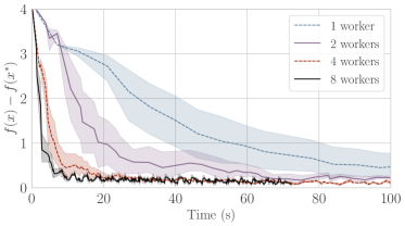
(b) Time vs. Objective

Figure 1: Convergence of AsyB-ProxSGD on the sparse logistic regression problem under different numbers of workers. In this figure, the number of servers is fixed to 8.

We now present numerical results to confirm that our proposed algorithms can be used to solve the challenging non-convex non-smooth problems in machine learning.

Setup: In our experiments, we consider the sparse logistic regression problem:

$$\mathop{\min}_{x}\frac{1}{n}\sum_{i=1}^{n}\log(1+\exp(-b_{i}\cdot a_{i}^{\top}x))+\lambda_{1}\lVert{x}\rVert+\frac{\lambda_{2}}{2}\lVert{x}\rVert^{2}.$$ (14)

The $\ell_{1}$-regularized logistic regression is widely used for large scale risk minimization. We consider the Avazu dataset , which is used in a click-through rate prediction competition jointly hosted by Avazu and Kaggle in 2014. In its training dataset (avazu-app), there are more than 14 million samples, 1 million features, and 4050 million nonzero entries. In other words, both $n$ and $d$ in (14) are large.

We use a cluster of 16 instances on Google Cloud. Each server or worker process uses just one core. Up to 8 instances serve as server nodes, while the other 8 instances serve as worker nodes. To show the advantage of asynchronous parallelism, we set up four experiments adopting 1, 2, 4, and 8 worker nodes, respectively. For all experiments, the whole dataset is shuffled and all workers have a copy of this dataset. When computing a stochastic gradient, each worker takes one minibatch of random samples from its own copy. This way, each sample is used by a worker with an equal probability empirically to mimic the scenario of our analysis.

We consider the suboptimality gap as our performance metric, which is defined as the gap between $f(x)$ and $f(x^{*})$. Here we estimate the optimal value $\hat{x}$ by performing $5\times$ as many iterations as needed for convergence. The hyper-parameters are set as follows. For all experiments, the coefficients are set as $\lambda_{1}=0.1$ and $\lambda_{2}=0.001$. We set the minibatch size to 8192. The step size is set according to $\eta_{k}:=0.1/\sqrt{1.0+k}$ at iteration $k\geq 0$.

Implementation:

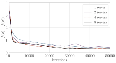
(a) Iteration vs. Objective

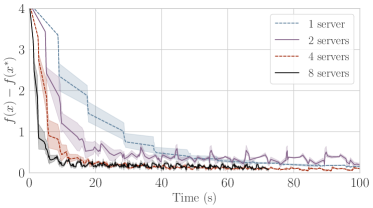
(b) Time vs. Objective

Figure 2: Convergence of AsyB-ProxSGD on the sparse logistic regression problem under different numbers of servers. In this figure, we use 8 workers with different numbers of servers.

We implemented our algorithm on MXNet Chen et al. (2015), a flexible and efficient deep learning library with support for distributed machine learning. Due to the sparse nature of the dataset, the model $x$ is stored as a sparse ndarray, and in each iteration, a worker only pulls those blocks of $x$ that are actively related to its sampled minibatch, and then calculates the gradient w.r.t. this minibatch of data, and pushes the gradients for those activated blocks only.

Results: Empirically, Assumption 4 (bounded delays) are observed to hold for this cluster. In our experiments, the maximum delay does not exceed 100 iterations unless some worker nodes fail. Fig. 1(a) and Fig. 1(b) show the convergence behavior of AsyB-ProxSGD algorithm in terms of objective function values. We can clearly observe the convergence of our proposed algorithm, confirming that asynchrony with tolerable delays can still lead to convergence. In addition, the running time drops in trend when the number of workers increases.

For our proposed AsyB-ProxSGD algorithm, we are particularly interested in two kinds of speedup, namely, iteration speedup and running time speedup. If we need $T_{1}$ iterations (with $T_{1}$ sample gradients processed by servers) to achieve a certain suboptimality level using one worker, and $T_{p}$ iterations to achieve the same level using $p$ workers, then the iteration speedup is defined as $p\times T_{1}/T_{p}$ Lian et al. (2015). Note that iterations are counted on the server side, which is actually the number of minibatch gradients are processed by the server. On the other hand, the time speedup is simply defined as the ratio between the running time of using one worker and that of using $p$ workers to achieve the same suboptimality level. We summarize iteration and running time speedup in Table 1.

Table 1: Iteration speedup and time speedup of AsyB-ProxSGD at the optimality level $10^{-1}$.

Workers	1	2	4	8
Iteration Speedup	1.000	2.127	3.689	6.748
Time Speedup	1.000	1.973	4.103	8.937

We further evaluate the relationship between the number of servers and the convergence behavior. Since the model has millions of parameters to be trained, storing the whole model in a single machine can be ineffective. In fact, from Fig. 2 we can even see nearly linear speedup w.r.t. the number of servers. The reason here is that, more servers can significantly decrease the length of request queue at the server side. When we have only one server, the blue dashed curve in Fig. 2(b) looks like a tilt staircase, and further investigation shows that some push requests take too long time to be processed. Therefore, we have to set more than one servers to observe parallel speedup in Fig. 1 so that servers are not the bottleneck.

6 Related Work

Robbins and Monro (1951) propose a classical stochastic approximation algorithm for solving a class of strongly convex problems, which is regarded as the seminal work of stochastic optimization problems. For nonconvex problems, Ghadimi and Lan (2013) prove that SGD has an ergodic convergence rate of $O(1/\sqrt{K})$, which is consistent with the convergence rate of SGD for convex problems. To deal with nonsmoothness, proximal gradient algorithm is widely considered and its stochastic variant is heavily studied for convex problems. Duchi and Singer (2009) show ProxSGD can converge at the rate of $O(1/\mu K)$ for $\mu$-strongly convex objective functions when the step size $\eta_{k}$ diminishes during iterations. However, for nonconvex problems, rather limited studies on ProxSGD exist so far. To our best knowledge, the seminal work on ProsSGD for nonconvex problems was done by Ghadimi et al. (2016), in which the convergence analysis is based on the assumption of an increasing minibatch size.

Updating a single block in each iteration is also referred to as block coordinate methods in the literature. Block coordinate methods for smooth problems with separable, convex constraints Tseng (1991) and general nonsmooth regularizers Razaviyayn et al. (2014); Davis (2016); Zhou et al. (2016) are proposed. However, the study on stochastic coordinate descent is limited and existing work like Liu and Wright (2015) focuses on convex problems. Xu and Yin (2015) study block stochastic proximal methods for nonconvex problems. However, they only analyze convergence to stationary points assuming an increasing minibatch size, and the convergence rate is not provided. Davis et al. (2016) presents a stochastic block coordinate method, which is the closest one with our work in this paper. However, the algorithm studied in Davis et al. (2016) depends on the use of a noise term with diminishing variance to guarantee convergence. Our convergence results of ProxSGD do not rely on the assumption of increasing batch sizes, variance reduction or the use of additional noise terms.

7 Concluding Remarks

In this paper, we propose AsyB-ProxSGD as an extension of the proximal stochastic gradient (ProxSGD) algorithm to asynchronous model parallelism setting. Our proposed algorithm aims at solving nonconvex nonsmooth optimization problems involved with large data size and model dimension. Theoretically, we prove that the AsyB-ProxSGD method has a convergence rate to critical points with the same order as ProxSGD, as long as workers have bounded delay during iterations. Our convergence result does not rely on minibatch size increasing, which is required in all existing works for ProxSGD (and its variants). We further prove that AsyB-ProxSGD can achieve linear speedup when the number of workers is bounded by $O(K^{1/4})$. We implement AsyB-ProxSGD on Parameter Server and experiments on large scale real-world dataset confirms its effectiveness.

Appendix A Auxiliary Lemmas

Lemma 2 (Ghadimi et al. [2016]).

For all $y\leftarrow\mathbf{prox}_{\eta h}(x-\eta g)$, we have:

$$\langle{g,y-x}\rangle+(h(y)-h(x))\leq-\frac{\lVert{y-x}\rVert_{2}^{2}}{\eta}.$$ (15)

Due to slightly different notations and definitions in Ghadimi et al. [2016], we provide a proof here for completeness. We refer readers to Ghadimi et al. [2016] for more details.

Proof.

By the definition of proximal function, there exists a $p\in\partial h(y)$ such that:

$$\begin{split}\langle{g+\frac{y-x}{\eta}+p,x-y}\rangle&\geq 0,\\ \langle{g,x-y}\rangle&\geq\frac{1}{\eta}\langle{y-x,y-x}\rangle+\langle{p,y-x}\rangle\\ \langle{g,x-y}\rangle+(h(x)-h(y))&\geq\frac{1}{\eta}\lVert{y-x}\rVert_{2}^{2},\end{split}$$

which proves the lemma.     $\sqcap$$\sqcup$

By applying the above lemma for each block, we have the following corollary, which is useful in convergence analysis for Algorithm LABEL:alg:abpsgd-global.

Corollary 2.

For all $y_{j}\leftarrow\mathbf{prox}_{\eta h_{j}}(x_{j}-\eta g_{j})$, we have:

$$\langle{g_{j},y_{j}-x_{j}}\rangle+(h_{j}(y_{j})-h_{j}(x_{j}))\leq-\frac{\lVert{y_{j}-x_{j}}\rVert_{2}^{2}}{\eta}.$$ (16)

Lemma 3 (Ghadimi et al. [2016]).

For all $x,g,G\in d$, if $h:d\to$ is a convex function, we have

$$\lVert{\mathbf{prox}_{\eta h}(x-\eta G)-\mathbf{prox}_{\eta h}(x-\eta g)}\rVert\leq\eta\lVert{G-g}\rVert.$$ (17)

Proof.

Let $y$ denote $\mathbf{prox}_{\eta h}(x-\eta G)$ and $z$ denote $\mathbf{prox}_{\eta h}(x-\eta g)$. By definition of the proximal operator, for all $u\in d$, we have

$$\langle{G+\frac{y-x}{\eta}+p,u-y}\rangle \geq 0,$$

$$\langle{g+\frac{z-x}{\eta}+q,u-z}\rangle \geq 0,$$

where $p\in\partial h(y)$ and $q\in\partial h(z)$. Let $z$ substitute $u$ in the first inequality and $y$ in the second one, we have

$$\langle{G+\frac{y-x}{\eta}+p,z-y}\rangle \geq 0,$$

$$\langle{g+\frac{z-x}{\eta}+q,y-z}\rangle \geq 0.$$

Then, we have

$$\langle{G,z-y}\rangle \geq\langle{\frac{y-x}{\eta},y-z}\rangle+\langle{p,y-z}\rangle,$$ (18)

$$=\frac{1}{\eta}\langle{y-z,y-z}\rangle+\frac{1}{\eta}\langle{z-x,y-z}\rangle+\langle{p,y-z}\rangle,$$ (19)

$$\geq\frac{\lVert{y-z}\rVert^{2}}{\eta}+\frac{1}{\eta}\langle{z-x,y-z}\rangle+h(y)-h(z),$$ (20)

and

$$\langle{g,y-z}\rangle \geq\langle{\frac{z-x}{\eta}+q,z-y}\rangle,$$ (21)

$$=\frac{1}{\eta}\langle{z-x,z-y}\rangle+\langle{q,z-y}\rangle$$ (22)

$$\geq\frac{1}{\eta}\langle{z-x,z-y}\rangle+h(z)-h(y).$$ (23)

By adding (20) and (23), we obtain

$$\lVert{G-g}\rVert\lVert{z-y}\rVert\geq\langle{G-g,z-y}\rangle\geq\frac{1}{\eta}\lVert{y-z}\rVert^{2},$$

which proves the lemma.     $\sqcap$$\sqcup$

Corollary 3.

For all $x_{j},g_{j},G_{j}\in d_{j}$, we have

$$\lVert{\mathbf{prox}_{\eta h_{j}}(x_{j}-\eta G_{j})-\mathbf{prox}_{\eta h_{j}}(x_{j}-\eta g_{j})}\rVert\leq\eta\lVert{G_{j}-g_{j}}\rVert.$$ (24)

Lemma 4 (Ghadimi et al. [2016]).

For any $g_{1}$ and $g_{2}$, we have

$$\lVert{P(x,g_{1},\eta)-P(x,g_{2},\eta)}\rVert\leq\lVert{g_{1}-g_{2}}\rVert.$$ (25)

Proof.

It can be obtained by directly applying Lemma 17 and the definition of gradient mapping.     $\sqcap$$\sqcup$

Corollary 4.

Let $P_{j}(x,g,\eta):=\frac{1}{\eta}(x_{j}-\mathbf{prox}_{\eta h_{j}}(x_{j}-\eta g_{j}))$. Then, for any $G_{j}$ and $g_{j}$, we have

$$\lVert{P_{j}(x,G,\eta)-P_{j}(x,g,\eta)}\rVert\leq\lVert{G-g}\rVert.$$ (26)

Lemma 5 (Reddi et al. [2016]).

Suppose we define $y=\mathbf{prox}_{\eta h}(x-\eta g)$ for some $g$. Then for $y$, the following inequality holds:

$$\begin{split}\Psi(y)\leq\Psi(z)+&\langle{y-z,\nabla f(x)-g}\rangle\\ &+\left(\frac{L}{2}-\frac{1}{2\eta}\right)\lVert{y-x}\rVert^{2}+\left(\frac{L}{2}+\frac{1}{2\eta}\right)\lVert{z-x}\rVert^{2}-\frac{1}{2\eta}\lVert{y-z}\rVert^{2},\end{split}$$ (27)

for all $z$.

Corollary 5.

Suppose we define $y_{j}=\mathbf{prox}_{\eta h_{j}}(x_{j}-\eta g_{j})$ for some $g_{j}$, and the index $j$ is chosen among $M$ indices with uniform distribution. For other $j^{\prime}\neq j$, we assume $y_{j^{\prime}}=x_{j^{\prime}}$. Then the following inequality holds:

$$\begin{split}\Psi(y)&\leq\Psi(z)+\langle{\nabla_{j}f(x)-g_{j},y_{j}-z_{j}}\rangle\\ &\quad\quad+\left(\frac{L_{j}}{2}-\frac{1}{2\eta}\right)\lVert{y_{j}-x_{j}}\rVert^{2}+\left(\frac{L_{j}}{2}+\frac{1}{2\eta}\right)\lVert{z_{j}-x_{j}}\rVert^{2}-\frac{1}{2\eta}\lVert{y_{j}-x_{j}}\rVert^{2}.\end{split}$$ (28)

for all $z$.

Proof.

From the definition of proximal operator, we have

$$\ \quad h_{j}(y_{j})+\langle{g_{j},y_{j}-x_{j}}\rangle+\frac{1}{2\eta}\lVert{y_{j}-x_{j}}\rVert^{2}+\frac{\eta}{2}\lVert{g_{j}}\rVert^{2}$$

$$\leq h_{j}(z_{j})+\langle{g_{j},z_{j}-x_{j}}\rangle+\frac{1}{2\eta}\lVert{z_{j}-x_{j}}\rVert^{2}+\frac{\eta}{2}\lVert{g_{j}}\rVert^{2}-\frac{1}{2\eta}\lVert{y_{j}-z_{j}}\rVert^{2}.$$

By rearranging the above inequality, we have

$$h_{j}(y_{j})+\langle{g_{j},y_{j}-z_{j}}\rangle\leq h_{j}(z_{j})+\frac{1}{2\eta}[\lVert{z_{j}-x_{j}}\rVert^{2}-\lVert{y_{j}-x_{j}}\rVert^{2}-\lVert{y_{j}-z_{j}}\rVert^{2}].$$ (29)

Since $f$ is $L$-Lipschitz, we have

$$f(y) \leq f(x)+\langle{\nabla_{j}f(x),y_{j}-x_{j}}\rangle+\frac{L_{j}}{2}\lVert{y_{j}-x_{j}}\rVert^{2},$$

$$f(x) \leq f(z)+\langle{\nabla_{j}f(x),x_{j}-z_{j}}\rangle+\frac{L_{j}}{2}\lVert{x_{j}-z_{j}}\rVert^{2}.$$

Adding these two inequality we have

$$f(y)\leq f(z)+\langle{\nabla_{j}f(x),y_{j}-z_{j}}\rangle+\frac{L}{2}[\lVert{y_{j}-x_{j}}\rVert^{2}+\lVert{z_{j}-x_{j}}\rVert^{2}],$$ (30)

and therefore

$$\Psi(y) \leq\Psi(z)+\langle{\nabla_{j}f(x)-g_{j},y_{j}-z_{j}}\rangle$$

$$\quad\quad+\left(\frac{L_{j}}{2}-\frac{1}{2\eta}\right)\lVert{y_{j}-x_{j}}\rVert^{2}+\left(\frac{L_{j}}{2}+\frac{1}{2\eta}\right)\lVert{z_{j}-x_{j}}\rVert^{2}-\frac{1}{2\eta}\lVert{y_{j}-x_{j}}\rVert^{2}.$$

$\sqcap$$\sqcup$

Lemma 6 (Young’s Inequality).

$$\langle{a,b}\rangle\leq\frac{1}{2\delta}\lVert{a}\rVert^{2}+\frac{\delta}{2}\lVert{b}\rVert^{2}.$$ (31)

We recall and define some notations for convergence analysis in the subsequent. We denote $\hat{G}_{j}^{k}$ as the average of delayed stochastic gradients and $\hat{g}_{j}^{k}$ as the average of delayed true gradients, respectively:

$$\hat{G}_{j}^{k} :=\frac{1}{N}\sum_{i=1}^{N}\nabla_{j}F(x_{j}^{k-\mathbf{d}_{k}};\xi_{k,i})$$

$$\hat{g}_{j}^{k} :=\frac{1}{N}\sum_{i=1}^{N}\nabla_{j}f(x_{j}^{k-\mathbf{d}_{k}}).$$

Moreover, we denote $\delta_{j}^{k}:=\hat{g}_{j}^{k}-\tilde{G}_{j}^{k}$ as the difference between these two differences.

Appendix B Convergence analysis for B-PAPSG

To simplify notations, we use $j$ instead of $j_{k}$ in this section. Since we update one block only in each iteration, we define an auxiliary function as follows:

$$P_{j}(x,g,\eta):=\frac{1}{\eta}(x_{j}-\mathbf{prox}_{\eta h_{j}}(x_{j}-\eta g_{j})),$$

where the variables $x_{j}$ and $g_{j}$ take the $j$-th coordinate.

B.1 Milestone Lemmas

Lemma 7 (Descent Lemma).

$$\mathbb{E}_{j}[\Psi(x^{k+1})|\mathcal{F}_{k}]\leq\mathbb{E}_{j}[\Psi(x^{k})|\mathcal{F}_{k}]-\frac{\eta_{k}-4L_{\max}\eta_{k}^{2}}{2M}\lVert{P(x^{k},\hat{g}^{k},\eta_{k})}\rVert^{2}+\frac{\eta_{k}}{2M}\lVert{g^{k}-\hat{g}^{k}}\rVert^{2}+\frac{L\eta_{k}^{2}}{MN}\sigma^{2}.$$ (32)

Lemma 8.

Suppose we have a sequence $\{x^{k}\}$ by Algorithm 2. Then, we have

$$\mathbb{E}[\lVert{x^{k}-x^{k-\tau}}\rVert^{2}]\leq\frac{2T\sum_{l=1}^{T}\eta_{k-l}^{2}}{MN}\sigma^{2}+2\left\lVert{\sum_{l\in K(\bm{\tau}(k))}\eta_{k-l}P_{j_{k-l}}(x^{k-l},\hat{g}^{k-l},\eta_{k-l})}\right\rVert^{2}$$ (33)

Lemma 9.

Suppose we have a sequence $\{x^{k}\}$ by Algorithm 2. Then, we have

$$\mathbb{E}[\lVert{g_{j}^{k}-\hat{g}_{j}^{k}}\rVert^{2}]\leq\frac{2L^{2}T\sum_{l=1}^{T}\eta_{k-l}^{2}}{M^{2}N}\sigma^{2}+\frac{2L^{2}T}{M^{2}}\sum_{l=1}^{T}\eta_{k-l}^{2}\lVert{P(x^{k-l},\hat{g}^{k-l},\eta_{k-l})}\rVert^{2}$$ (34)

B.2 Proof of Theorem 1

Proof.

We have

$$\lVert{P_{j}(x_{k},\hat{g}_{k},\eta_{k})}\rVert^{2}\geq\frac{1}{2}\lVert{P_{j}(x_{k},g_{k},\eta_{k})}\rVert^{2}-\lVert{g_{k}-\hat{g}_{k}}\rVert^{2}.$$

When we have $\eta_{k}\leq\frac{1}{8L_{\max}}$, we can apply the above equation following Lemma 32:

$$\quad\ \mathbb{E}_{j}[\Psi(x^{k+1})|\mathcal{F}_{k}]$$

$$\leq\mathbb{E}_{j}[\Psi(x^{k})|\mathcal{F}_{k}]-\frac{\eta_{k}-4L_{\max}\eta_{k}^{2}}{2M}\lVert{P(x^{k},\hat{g}^{k},\eta_{k})}\rVert^{2}+\frac{\eta_{k}}{2M}\lVert{g^{k}-\hat{g}^{k}}\rVert^{2}+\frac{L\eta_{k}^{2}}{MN}\sigma^{2}$$

$$\leq\mathbb{E}_{j}[\Psi(x^{k})|\mathcal{F}_{k}]-\frac{\eta_{k}-8L_{\max}\eta_{k}^{2}}{4M}\lVert{P(x^{k},\hat{g}^{k},\eta_{k})}\rVert^{2}-\frac{\eta_{k}}{4M}\lVert{P(x^{k},\hat{g}^{k},\eta_{k})}\rVert^{2}$$

$$\quad\ +\frac{\eta_{k}}{2M}\lVert{g^{k}-\hat{g}^{k}}\rVert^{2}+\frac{L\eta_{k}^{2}}{MN}\sigma^{2}$$

$$\leq\mathbb{E}_{j}[\Psi(x^{k})|\mathcal{F}_{k}]-\frac{\eta_{k}-8L_{\max}\eta_{k}^{2}}{8M}\lVert{P(x^{k},g^{k},\eta_{k})}\rVert^{2}+\frac{3\eta_{k}}{4M}\lVert{g^{k}-\hat{g}^{k}}\rVert^{2}$$

$$\quad\ -\frac{\eta_{k}}{4M}\lVert{P(x^{k},\hat{g}^{k},\eta_{k})}\rVert^{2}+\frac{L\eta_{k}^{2}}{MN}\sigma^{2}$$

By Lemma 34, we have

$$\quad\ \mathbb{E}_{j}[\Psi(x^{k+1})|\mathcal{F}_{k}]$$

$$\leq\mathbb{E}_{j}[\Psi(x^{k})|\mathcal{F}_{k}]-\frac{\eta_{k}-8L_{\max}\eta_{k}^{2}}{8M}\lVert{P(x^{k},g^{k},\eta_{k})}\rVert^{2}-\frac{\eta_{k}}{4M}\lVert{P(x^{k},\hat{g}^{k},\eta_{k})}\rVert^{2}+\frac{L\eta_{k}^{2}}{MN}\sigma^{2}$$

$$\quad+\frac{3\eta_{k}}{4M}\left(\frac{2L^{2}T\sum_{l=1}^{T}\eta_{k-l}^{2}}{M^{2}N}\sigma^{2}+\frac{2L^{2}T}{M^{2}}\sum_{l=1}^{T}\eta_{k-l}^{2}\lVert{P(x^{k-l},\hat{g}^{k-l},\eta_{k-l})}\rVert^{2}\right)$$

$$\leq\mathbb{E}_{j}[\Psi(x^{k})|\mathcal{F}_{k}]-\frac{\eta_{k}-8L_{\max}\eta_{k}^{2}}{8M}\lVert{P(x^{k},g^{k},\eta_{k})}\rVert^{2}+\left(\frac{L\eta_{k}^{2}}{MN}+\frac{3\eta_{k}L^{2}T\sum_{l=1}^{T}\eta_{k-l}^{2}}{2M^{3}N}\right)\sigma^{2}$$

$$\quad+\frac{3\eta_{k}L^{2}T}{2M^{3}}\sum_{l=1}^{T}\eta_{k-l}^{2}\lVert{P_{j_{k-l}}(x^{k-l},\hat{g}^{k-l},\eta_{k-l})}\rVert^{2}-\frac{\eta_{k}}{4M}\lVert{P(x^{k},\hat{g}^{k},\eta_{k})}\rVert^{2}$$

By taking telescope sum, we have

$$\quad\ \sum_{k=1}^{K}\frac{\eta_{k}-8L_{\max}\eta_{k}^{2}}{8M}\lVert{P(x^{k},g^{k},\eta_{k})}\rVert^{2}$$

$$\leq\Psi(x^{1})-\Psi(x^{*})+\sum_{k=1}^{K}\left(\frac{L\eta_{k}^{2}}{MN}+\frac{3\eta_{k}L^{2}T\sum_{l=1}^{T}\eta_{k-l}^{2}}{2M^{3}N}\right)\sigma^{2}$$

$$\quad-\sum_{k=1}^{K}(\frac{\eta_{k}}{4M}-\frac{3\eta_{k}^{2}L^{2}}{2M^{3}}\sum_{l=1}^{l_{k}}\eta_{k+l}^{2})\lVert{P(x^{k},\hat{g}^{k},\eta_{k})}\rVert^{2}$$

$$\leq\Psi(x^{1})-\Psi(x^{*})+\sum_{k=1}^{K}\left(\frac{L\eta_{k}^{2}}{MN}+\frac{3\eta_{k}L^{2}T\sum_{l=1}^{T}\eta_{k-l}^{2}}{2M^{3}N}\right)\sigma^{2},$$

where the last inequality follows from the assumption that $6\eta_{k}^{2}L^{2}\sum_{l=1}^{T}\eta_{k+l}\leq M^{2}$, and now we prove Theorem 1.

$\sqcap$$\sqcup$

B.3 Proof of Corollary 13

Proof.

Since the learning rate $\eta_{k}:=\eta$ is a constant, we apply it to Theorem 1 and we have:

$$\frac{1}{K}\sum_{k=1}^{K}\mathbb{E}[\lVert{P(x^{k},g^{k},\eta_{k})}\rVert^{2}]\leq\frac{16M(\Psi(x^{1})-\Psi(x^{*}))}{K\eta}+\frac{16M}{\eta}\left(\frac{L\eta^{2}}{MN}+\frac{3L^{2}T^{2}\eta^{3}}{2M^{3}N}\right)\sigma^{2}.$$ (35)

Following conditions in Corollary 13, we have

$$\eta\leq\frac{M^{2}}{16L(T+1)^{2}},$$

and thus we have

$$\frac{3LT^{2}\eta}{2M^{2}} \leq\frac{3M^{2}T^{2}}{2M^{2}\cdot 16(T+1)^{2}}\leq 1,$$

$$\frac{3L^{2}T^{2}\eta^{3}}{2M^{2}} \leq L\eta^{2}.$$

Then, we can estimate (35) from the above inequality as follows:

$$\frac{1}{K}\sum_{k=1}^{K}\mathbb{E}[\lVert{P(x^{k},g^{k},\eta_{k})}\rVert^{2}] \leq\frac{16M(\Psi(x^{1})-\Psi(x^{*}))}{K\eta}+\frac{16M}{\eta}\left(\frac{L\eta^{2}}{MN}+\frac{3L^{2}T^{2}\eta^{3}}{2M^{3}N}\right)\sigma^{2}$$

$$\leq\frac{16M(\Psi(x^{1})-\Psi(x^{*}))}{K\eta}+\frac{32L\eta}{N}\sigma^{2}$$

$$=32\sqrt{\frac{2(\Psi(x^{1})-\Psi(x^{*}))LM(T+1)\sigma^{2}}{KN}},$$

which proves the corollary.     $\sqcap$$\sqcup$

B.4 Proof of Milestone Lemmas

Proof of Lemma 32.

Recall Corollary 5:

$$\Psi(x^{k+1}) \leq\Psi(\bar{x}^{k+1})+\langle{\nabla_{j}f(x^{k})-\hat{G}_{j}^{k},x_{j}^{k+1}-\bar{x}_{j}^{k+1}}\rangle$$

$$\quad\quad+\left(\frac{L_{j}}{2}-\frac{1}{2\eta}\right)\lVert{y_{j}-x_{j}}\rVert^{2}+\left(\frac{L_{j}}{2}+\frac{1}{2\eta}\right)\lVert{z_{j}-x_{j}}\rVert^{2}-\frac{1}{2\eta}\lVert{y_{j}-x_{j}}\rVert^{2}.$$

Now we turn to bound $\Psi(\bar{x}_{j}^{k+1})$ as follows:

$$\begin{split}&\quad\ f(\bar{x}^{k+1})\\ &\leq f(x^{k})+\langle{\nabla_{j}f(x^{k}),\bar{x}_{j}^{k+1}-x_{j}^{k}}\rangle+\frac{L_{j}}{2}\lVert{\bar{x}_{j}^{k+1}-x_{j}^{k}}\rVert^{2}\\ &=f(x^{k})+\langle{g_{j}^{k},\bar{x}_{j}^{k+1}-x_{j}^{k}}\rangle+\frac{\eta_{k}^{2}L_{j}}{2}\lVert{P_{j}(x^{k},\hat{g}^{k},\eta_{k})}\rVert^{2}\\ &=f(x^{k})+\langle{\hat{g}_{j}^{k},\bar{x}_{j}^{k+1}-x_{j}^{k}}\rangle+\langle{g_{j}^{k}-\hat{g}_{j}^{k},\bar{x}_{j}^{k+1}-x_{j}^{k}}\rangle+\frac{\eta_{k}^{2}L_{j}}{2}\lVert{P_{j}(x^{k},\hat{g}^{k},\eta_{k})}\rVert^{2}\\ &=f(x^{k})-\eta_{k}\langle{\hat{g}_{j}^{k},P_{j}(x^{k},\hat{g}_{j}^{k},\eta_{k})}\rangle+\langle{g_{j}^{k}-\hat{g}_{j}^{k},\bar{x}_{j}^{k+1}-x_{j}^{k}}\rangle+\frac{\eta_{k}^{2}L_{j}}{2}\lVert{P_{j}(x^{k},\hat{g}^{k},\eta_{k})}\rVert^{2}\\ &\leq f(x^{k})-[\eta_{k}\lVert{P_{j}(x^{k},\hat{g}^{k},\eta_{k})}\rVert^{2}+h_{j}(\bar{x}_{j}^{k+1})-h_{j}(x_{j}^{k})]\\ &\quad\ +\langle{g_{j}^{k}-\hat{g}_{j}^{k},\bar{x}_{j}^{k+1}-x_{j}^{k}}\rangle+\frac{\eta_{k}^{2}L_{j}}{2}\lVert{P_{j}(x^{k},\hat{g}^{k},\eta_{k})}\rVert^{2},\end{split}$$

where the last inequality follows from Corollary 16. By rearranging terms on both sides, we have

$$\Psi(\bar{x}^{k+1})\leq\Psi(x^{k})-(\eta_{k}-\frac{\eta_{k}^{2}L_{j}}{2})\lVert{P_{j}(x^{k},\hat{g}^{k},\eta_{k})}\rVert^{2}+\langle{g_{j}^{k}-\hat{g}_{j}^{k},\bar{x}_{j}^{k+1}-x_{j}^{k}}\rangle$$ (36)

Taking the summation of (LABEL:eq:yk_baryk_async) and (36), we have

$$\begin{split}&\quad\ \Psi(x^{k+1})\\ &\leq\Psi(x^{k})+\langle{\nabla_{j}f(x^{k})-\hat{G}_{j}^{k},x_{j}^{k+1}-\bar{x}_{j}^{k+1}}\rangle\\ &\quad+\left(\frac{L_{j}}{2}-\frac{1}{2\eta}\right)\lVert{y_{j}-x_{j}}\rVert^{2}+\left(\frac{L_{j}}{2}+\frac{1}{2\eta_{k}}\right)\lVert{z_{j}-x_{j}}\rVert^{2}-\frac{1}{2\eta_{k}}\lVert{y_{j}-x_{j}}\rVert^{2}\\ &\quad-(\eta_{k}-\frac{\eta_{k}^{2}L_{j}}{2})\lVert{P_{j}(x^{k},\hat{g}_{k},\eta_{k})}\rVert^{2}+\langle{g_{j}^{k}-\hat{g}_{j}^{k},\bar{x}_{j}^{k+1}-x_{j}^{k}}\rangle\\ &=\Psi(x^{k})+\langle{\nabla_{j}f(x^{k})-\hat{g}_{j}^{k},x_{j}^{k+1}-\bar{x}_{j}^{k+1}}\rangle+\langle{\hat{g}_{j}^{k}-\hat{G}_{j}^{k},x_{j}^{k+1}-\bar{x}_{j}^{k+1}}\rangle\\ &\quad+\left(\frac{L_{j}\eta_{k}^{2}}{2}-\frac{\eta_{k}}{2}\right)\lVert{P_{j}(x^{k},\hat{G}^{k},\eta_{k})}\rVert^{2}+\left(\frac{L_{j}\eta_{k}^{2}}{2}+\frac{\eta_{k}}{2}\right)\lVert{P_{j}(x^{k},\hat{g}^{k},\eta_{k})}\rVert^{2}\\ &\quad-\frac{1}{2\eta_{k}}\lVert{x_{j}^{k+1}-\bar{x}_{j}^{k+1}}\rVert^{2}-(\eta_{k}-\frac{\eta_{k}^{2}L_{j}}{2})\lVert{P_{j}(x^{k},\hat{g}^{k},\eta_{k})}\rVert^{2}\\ &=\Psi(x^{k})+\langle{x_{j}^{k+1}-x_{j}^{k},g_{j}^{k}-\hat{g}_{j}^{k}}\rangle+\langle{x_{j}^{k+1}-\bar{x}_{j}^{k+1},\delta_{j}^{k}}\rangle+\frac{L_{j}\eta_{k}^{2}-\eta_{k}}{2}\lVert{P_{j}(x^{k},\hat{G}^{k},\eta_{k})}\rVert^{2}\\ &\quad+\frac{2L_{j}\eta_{k}^{2}-\eta_{k}}{2}\lVert{P_{j}(x^{k},\hat{g}^{k},\eta_{k})}\rVert^{2}-\frac{1}{2\eta_{k}}\lVert{x_{j}^{k+1}-\bar{x}_{j}^{k+1}}\rVert^{2}.\end{split}$$

By taking the expectation on condition of filtration $\mathcal{F}_{k}$ and $j$, we have the following equation according to Assumption 2:

$$\begin{split}&\quad\ \mathbb{E}_{j}[\Psi(x^{k+1})|\mathcal{F}_{k}]\\ &\leq\mathbb{E}_{j}[\Psi(x^{k})|\mathcal{F}_{k}]+\frac{1}{M}\mathbb{E}[\langle{x^{k+1}-x^{k},g^{k}-\hat{g}_{k}}\rangle|\mathcal{F}_{k}]+\frac{L_{\max}\eta_{k}^{2}-\eta_{k}}{2M}\mathbb{E}[\lVert{P(x^{k},\hat{G}^{k},\eta_{k})}\rVert^{2}|\mathcal{F}_{k}]\\ &\quad+\frac{2L_{\max}\eta_{k}^{2}-\eta_{k}}{2M}\lVert{P(x^{k},\hat{g}^{k},\eta_{k})}\rVert^{2}-\frac{1}{2M\eta_{k}}\lVert{x^{k+1}-\bar{x}^{k+1}}\rVert^{2}.\end{split}$$ (37)

Therefore, we have

$$\begin{split}&\quad\ \mathbb{E}_{j}[\Psi(x^{k+1})|\mathcal{F}_{k}]\\ &\leq\mathbb{E}_{j}[\Psi(x^{k})|\mathcal{F}_{k}]+\frac{1}{M}\mathbb{E}[\langle{x^{k+1}-x^{k},g^{k}-\hat{g}^{k}}\rangle|\mathcal{F}_{k}]+\frac{L_{\max}\eta_{k}^{2}-\eta_{k}}{2M}\mathbb{E}[\lVert{P(x^{k},\hat{G}^{k},\eta_{k})}\rVert^{2}|\mathcal{F}_{k}]\\ &\quad+\frac{2L_{\max}\eta_{k}^{2}-\eta_{k}}{2M}\lVert{P(x^{k},\hat{g}^{k},\eta_{k})}\rVert^{2}-\frac{1}{2M\eta_{k}}\lVert{x^{k+1}-\bar{x}^{k+1}}\rVert^{2}\\ &\leq\mathbb{E}_{j}[\Psi(x^{k})|\mathcal{F}_{k}]+\frac{\eta_{k}}{2M}\lVert{g^{k}-\hat{g}^{k}}\rVert^{2}+\frac{L_{\max}\eta_{k}^{2}}{2M}\mathbb{E}[\lVert{P(x^{k},\hat{G}^{k},\eta_{k})}\rVert^{2}|\mathcal{F}_{k}]+\frac{2L_{\max}\eta_{k}^{2}-\eta_{k}}{2M}\lVert{P(x^{k},\hat{g}^{k},\eta_{k})}\rVert^{2}\\ &\leq\mathbb{E}_{j}[\Psi(x^{k})|\mathcal{F}_{k}]\\ &\quad\ -\frac{\eta_{k}-4L_{\max}\eta_{k}^{2}}{2M}\lVert{P(x^{k},\hat{g}^{k},\eta_{k})}\rVert^{2}+\frac{\eta_{k}}{2M}\lVert{g^{k}-\hat{g}^{k}}\rVert^{2}+\frac{L\eta_{k}^{2}}{MN}\sigma^{2}.\end{split}$$

$\sqcap$$\sqcup$

Proof of Lemma 33.

$$\lVert{x^{k}-x^{k-\tau}}\rVert^{2} =\left\lVert{\sum_{l\in K(\bm{\tau}(k))}x^{k-l+1}-x^{k-l}}\right\rVert^{2}$$

$$=\left\lVert{\sum_{l\in K(\bm{\tau}(k))}\eta_{k-l}P_{j_{k-l}}(x^{k-l},\hat{G}^{k-l},\eta_{k-l})}\right\rVert^{2}$$

$$\leq 2\left\lVert{\sum_{l\in K(\bm{\tau}(k))}\eta_{k-l}(P_{j_{k-l}}(x^{k-l},\hat{G}^{k-l},\eta_{k-l})-P_{j_{k-l}}(x^{k-l},\hat{g}^{k-l},\eta_{k-l}))}\right\rVert^{2}$$

$$\quad+2\left\lVert{\sum_{l\in K(\bm{\tau}(k))}\eta_{k-l}P_{j_{k-l}}(x^{k-l},\hat{g}^{k-l},\eta_{k-l})}\right\rVert^{2}$$

$$\leq 2T\sum_{l\in K(\bm{\tau}(k))}\eta_{k-l}^{2}\left\lVert{P_{j_{k-l}}(x^{k-l},\hat{G}^{k-l},\eta_{k-l})-P_{j_{k-l}}(x^{k-l},\hat{g}^{k-l},\eta_{k-l})}\right\rVert^{2}$$

$$\quad+2\left\lVert{\sum_{l\in K(\bm{\tau}(k))}\eta_{k-l}P_{j_{k-l}}(x^{k-l},\hat{g}^{k-l},\eta_{k-l})}\right\rVert^{2}$$

$$\leq 2T\sum_{l=1}^{T}\eta_{k-l}^{2}\lVert{\hat{G}^{k-l}-\hat{g}^{k-l}}\rVert^{2}+2\left\lVert{\sum_{l\in K(\bm{\tau}(k))}\eta_{k-l}P_{j_{k-l}}(x^{k-l},\hat{g}^{k-l},\eta_{k-l})}\right\rVert^{2}$$

$$\leq\frac{2T\sum_{l=1}^{T}\eta_{k-l}^{2}}{MN}\sigma^{2}+2\left\lVert{\sum_{l\in K(\bm{\tau}(k))}\eta_{k-l}P_{j_{k-l}}(x^{k-l},\hat{g}^{k-l},\eta_{k-l})}\right\rVert^{2}$$

$\sqcap$$\sqcup$

Proof of Lemma 34.

$$\mathbb{E}[\lVert{g_{j}^{k}-\hat{g}_{j}^{k}}\rVert^{2}] =\left\lVert{\frac{1}{N}\sum_{i=1}^{N}g_{j}^{k}-\hat{g}_{j}^{k-\tau(k,i)}}\right\rVert^{2}$$

$$\leq\frac{1}{N}\sum_{i=1}^{N}\lVert{g_{j}^{k}-\hat{g}_{j}^{k-\tau(k,i)}}\rVert^{2}$$

$$\leq\frac{1}{MN}\sum_{i=1}^{N}\lVert{g^{k}-\hat{g}^{k-\tau(k,i)}}\rVert^{2}$$

$$\leq\frac{L^{2}}{MN}\sum_{i=1}^{N}\lVert{x^{k}-\hat{x}^{k-\tau(k,i)}}\rVert^{2}$$

$$\leq\frac{L^{2}}{MN}\sum_{i=1}^{N}\left(\frac{2T\sum_{l=1}^{T}\eta_{k-l}^{2}}{MN}\sigma^{2}+2\left\lVert{\sum_{l=1}^{T}\eta_{k-l}P_{j_{k-l}}(x^{k-l},\hat{g}^{k-l},\eta_{k-l})}\right\rVert^{2}\right)$$

$$\leq\frac{2L^{2}T\sum_{l=1}^{T}\eta_{k-l}^{2}}{M^{2}N}\sigma^{2}+\frac{2L^{2}T}{M^{2}}\sum_{l=1}^{T}\eta_{k-l}^{2}\lVert{P(x^{k-l},\hat{g}^{k-l},\eta_{k-l})}\rVert^{2}$$

$\sqcap$$\sqcup$

References

• Agarwal and Duchi [2011] A. Agarwal and J. C. Duchi. Distributed delayed stochastic optimization. In Advances in Neural Information Processing Systems, pages 873–881, 2011.
• Attouch et al. [2013] H. Attouch, J. Bolte, and B. F. Svaiter. Convergence of descent methods for semi-algebraic and tame problems: proximal algorithms, forward–backward splitting, and regularized gauss–seidel methods. Mathematical Programming, 137(1-2):91–129, 2013.
• Avron et al. [2015] H. Avron, A. Druinsky, and A. Gupta. Revisiting asynchronous linear solvers: Provable convergence rate through randomization. Journal of the ACM (JACM), 62(6):51, 2015.
• Borthakur et al. [2008] D. Borthakur et al. Hdfs architecture guide. Hadoop Apache Project, 53, 2008.
• Chen et al. [2015] T. Chen, M. Li, Y. Li, M. Lin, N. Wang, M. Wang, T. Xiao, B. Xu, C. Zhang, and Z. Zhang. Mxnet: A flexible and efficient machine learning library for heterogeneous distributed systems. arXiv preprint arXiv:1512.01274, 2015.
• Davis [2016] D. Davis. The asynchronous palm algorithm for nonsmooth nonconvex problems. arXiv preprint arXiv:1604.00526, 2016.
• Davis et al. [2016] D. Davis, B. Edmunds, and M. Udell. The sound of apalm clapping: Faster nonsmooth nonconvex optimization with stochastic asynchronous palm. In Advances in Neural Information Processing Systems, pages 226–234, 2016.
• Dean et al. [2012] J. Dean, G. Corrado, R. Monga, K. Chen, M. Devin, M. Mao, A. Senior, P. Tucker, K. Yang, Q. V. Le, et al. Large scale distributed deep networks. In Advances in neural information processing systems, pages 1223–1231, 2012.
• Duchi and Singer [2009] J. Duchi and Y. Singer. Efficient online and batch learning using forward backward splitting. Journal of Machine Learning Research, 10(Dec):2899–2934, 2009.
• Friedman et al. [2001] J. Friedman, T. Hastie, and R. Tibshirani. The elements of statistical learning, volume 1. Springer series in statistics Springer, Berlin, 2001.
• Ghadimi and Lan [2013] S. Ghadimi and G. Lan. Stochastic first-and zeroth-order methods for nonconvex stochastic programming. SIAM Journal on Optimization, 23(4):2341–2368, 2013.
• Ghadimi et al. [2016] S. Ghadimi, G. Lan, and H. Zhang. Mini-batch stochastic approximation methods for nonconvex stochastic composite optimization. Mathematical Programming, 155(1-2):267–305, 2016.
• Ho et al. [2013] Q. Ho, J. Cipar, H. Cui, S. Lee, J. K. Kim, P. B. Gibbons, G. A. Gibson, G. Ganger, and E. P. Xing. More effective distributed ml via a stale synchronous parallel parameter server. In Advances in neural information processing systems, pages 1223–1231, 2013.
• Hong et al. [2016] M. Hong, Z.-Q. Luo, and M. Razaviyayn. Convergence analysis of alternating direction method of multipliers for a family of nonconvex problems. SIAM Journal on Optimization, 26(1):337–364, 2016.
• Li and Lin [2015] H. Li and Z. Lin. Accelerated proximal gradient methods for nonconvex programming. In Advances in neural information processing systems, pages 379–387, 2015.
• Li et al. [2014a] M. Li, D. G. Andersen, J. W. Park, A. J. Smola, A. Ahmed, V. Josifovski, J. Long, E. J. Shekita, and B.-Y. Su. Scaling distributed machine learning with the parameter server. In 11th USENIX Symposium on Operating Systems Design and Implementation (OSDI 14), pages 583–598, 2014a.
• Li et al. [2014b] M. Li, D. G. Andersen, A. J. Smola, and K. Yu. Communication efficient distributed machine learning with the parameter server. In Advances in Neural Information Processing Systems, pages 19–27, 2014b.
• Li et al. [2016] M. Li, Z. Liu, A. J. Smola, and Y.-X. Wang. Difacto: Distributed factorization machines. In Proceedings of the Ninth ACM International Conference on Web Search and Data Mining, pages 377–386. ACM, 2016.
• Lian et al. [2015] X. Lian, Y. Huang, Y. Li, and J. Liu. Asynchronous parallel stochastic gradient for nonconvex optimization. In Advances in Neural Information Processing Systems, pages 2737–2745, 2015.
• Liu and Wright [2015] J. Liu and S. J. Wright. Asynchronous stochastic coordinate descent: Parallelism and convergence properties. SIAM Journal on Optimization, 25(1):351–376, 2015.
• Liu et al. [2009] J. Liu, J. Chen, and J. Ye. Large-scale sparse logistic regression. In Proceedings of the 15th ACM SIGKDD international conference on Knowledge discovery and data mining, pages 547–556. ACM, 2009.
• Mania et al. [2017] H. Mania, X. Pan, D. Papailiopoulos, B. Recht, K. Ramchandran, and M. I. Jordan. Perturbed iterate analysis for asynchronous stochastic optimization. SIAM Journal on Optimization, 27(4):2202–2229, jan 2017. doi: 10.1137/16m1057000. URL https://doi.org/10.1137%2F16m1057000.
• Niu et al. [2011] F. Niu, B. Recht, C. Re, and S. Wright. Hogwild: A lock-free approach to parallelizing stochastic gradient descent. In Advances in Neural Information Processing Systems, pages 693–701, 2011.
• Pan et al. [2016] X. Pan, M. Lam, S. Tu, D. Papailiopoulos, C. Zhang, M. I. Jordan, K. Ramchandran, and C. Ré. Cyclades: Conflict-free asynchronous machine learning. In Advances in Neural Information Processing Systems, pages 2568–2576, 2016.
• Parikh et al. [2014] N. Parikh, S. Boyd, et al. Proximal algorithms. Foundations and Trends® in Optimization, 1(3):127–239, 2014.
• Razaviyayn et al. [2014] M. Razaviyayn, M. Hong, Z.-Q. Luo, and J.-S. Pang. Parallel successive convex approximation for nonsmooth nonconvex optimization. In Advances in Neural Information Processing Systems, pages 1440–1448, 2014.
• Reddi et al. [2016] S. J. Reddi, S. Sra, B. Póczos, and A. J. Smola. Proximal stochastic methods for nonsmooth nonconvex finite-sum optimization. In Advances in Neural Information Processing Systems, pages 1145–1153, 2016.
• Robbins and Monro [1951] H. Robbins and S. Monro. A stochastic approximation method. The annals of mathematical statistics, pages 400–407, 1951.
• Sun and Luo [2015] R. Sun and Z.-Q. Luo. Guaranteed matrix completion via nonconvex factorization. In Foundations of Computer Science (FOCS), 2015 IEEE 56th Annual Symposium on, pages 270–289. IEEE, 2015.
• Tibshirani et al. [2005] R. Tibshirani, M. Saunders, S. Rosset, J. Zhu, and K. Knight. Sparsity and smoothness via the fused lasso. Journal of the Royal Statistical Society: Series B (Statistical Methodology), 67(1):91–108, 2005.
• Tseng [1991] P. Tseng. On the rate of convergence of a partially asynchronous gradient projection algorithm. SIAM Journal on Optimization, 1(4):603–619, 1991.
• Xu et al. [2010] H. Xu, C. Caramanis, and S. Sanghavi. Robust pca via outlier pursuit. In Advances in Neural Information Processing Systems, pages 2496–2504, 2010.
• Xu and Yin [2015] Y. Xu and W. Yin. Block stochastic gradient iteration for convex and nonconvex optimization. SIAM Journal on Optimization, 25(3):1686–1716, 2015.
• Zhang et al. [2015] S. Zhang, A. E. Choromanska, and Y. LeCun. Deep learning with elastic averaging sgd. In Advances in Neural Information Processing Systems, pages 685–693, 2015.
• Zhou et al. [2016] Y. Zhou, Y. Yu, W. Dai, Y. Liang, and E. Xing. On convergence of model parallel proximal gradient algorithm for stale synchronous parallel system. In Artificial Intelligence and Statistics, pages 713–722, 2016.