Experimental investigation of water jets under gravity

Abstract

The Plateau-Rayleigh theory essentially explains the breakup of liquid jets as due to growing perturbations along the length of the jet. The essential idea is supported by several experiments carried out in the past. Recently, the existence of a feedback mechanism in the form of recoil capillary waves was proposed to enhance the effect of the perturbations. We experimentally verify the existence of such recoil capillary waves. Using our experimental setup we further show that the wavy nature of the jet surface appears almost right after the emergence of the jet from the nozzle irrespective of the recoil capillary wave feedback. Moreover, our experimental results indicate existence of a sharp boundary, along the length of the continuous jet, beyond which gravitational effect dominates over the surface tension.

I Introduction

There have been many attempts theoretically as well as experimentally to understand the physical mechanism behind the breaking up of continuous jets into drops. However, the study of this macroscopic phenomenon continues to be of current interestEggers1 ; Eggers2 ; Lin ; Lautrup .

The problem of instability of liquid jets was investigated by Plateau and then by Rayleigh and developed a theory which came to be known as Plateau-Rayleigh theory. RayleighRay1 ; Ray2 , based on surface energy considerations of inviscid liquids, showed that perturbations of wavelengths $\lambda$ larger than $\pi$ times the jet diameter $d_{1}$ grow rapidly with time. However, it is the fastest growing perturbation ($\lambda\approx 4.508\times d_{1}$) that ultimately makes the jet column unstable against formation of droplets. ChandrasekharChandra later extended the theory to viscous liquids. Many experimental investigations have been conducted to examine the validity of Plateau-Rayleigh theory. The experiment of Goedde and Yuen, for example, applied external perturbations to study the length of the liquid jet before it breaks upGoedde .

In some recent works, Umemura and co-workersUmemura1 ; Umemura2 ; Umemura3 ; Umemura4 emphasized the idea that soon after the jet breaks up the new tip of the remaining column contracts to make its shape round once again to minimize its surface energy. The tip contraction (recoil) gives rise to upstream propagating capillary waves which upon reflection at the mouth of the nozzle move downstream with Doppler modified wavelengths. These feedback perturbations superpose with the preexisting perturbations and move down along the jet as combined perturbations. Some of these combined perturbations with the right wavelength cause the liquid column to breakup producing another contraction of the tip of the column and so on.

II Experimental set up and experiment

We set up and conduct an experiment to verify the existence and effect of the recoil capillary waves on the length of continuous water jet. We achieve this by damping the recoil capillary waves by bringing the jet in contact with a liquid surface beneath it. Moreover, when the continuous water jet smoothly merges into the water it creates ripples on the water surface in the beaker. Surface waves are observed using photographic methods and infer about the surface shape profile of the jet all along its length.

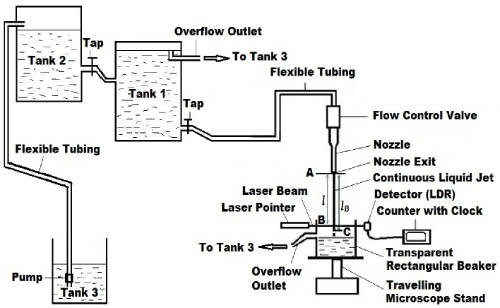
Figure 1: A sketch of the experimental set up.

Our experimental set up is similar in essentials to that of Goedde and YuenGoedde . The new and important addition is the intervening water containing beaker, Fig. 1. The details are given in Ref.Bani . The transparent rectangular beaker with a level outlet on one of its vertical sides is placed vertically below the nozzle so that the water jet falls directly on (or smoothly merges into) the water kept in the beaker. The water level in the beaker is maintained fixed by letting the excess water flow out through the level outlet. The beaker is placed on a horizontal platform fitted to the vertical stand of a travelling microscope (vernier scale least count = 0.001 cm) so that the beaker can be smoothly moved vertically and its position measured. A vertical-height adjustable laser-pointer-and-detector arrangement is also fitted to the platform so that the horizontal laser beam is incident normally on the vertical surface of the beaker and passes through the path of the water jet and then through the opposite surface of the beaker before it is collected by the detector. A digital counterDetails with a clock is connected to the detector to count the number of discontinuities in the water jet over a period of time.

Distilled water is issued vertically downward through a long glass nozzle (of length larger than about ten times its internal diameter $d$) in to the water in the beaker. The water flow rate is measured manually by collecting the jet water on a measuring cylinder for two minutes and calculating the mean value. As long as the jet remains continuous, at the level of the laser beam, the detector remains quiescent. However, a discontinuity in the jet after breakup allows the laser beam to pass through unobstructed and detected as a water drop count. We call the vertical distance between the mouth of the nozzle and the position of the laser beam as the jet-length, $l$. The vertical distance between the nozzle exit and the position of breakup of the jet, as detected by the laser-beam-counter, gives the breakup length, $l=l_{B}$.

Initially, the laser beam is made to face the continuous jet by moving the platform up closer to the nozzle, $l\approx 0$, and then the platform is gradually lowered in small steps so that $l$ increases. For each value of $l$, the number of counts is recorded for two minutes each for several times and their average calculated to obtain the mean drop-count rate. Naturally, the count rate begins from zero (at a threshold value of $l$) and then gradually keeps increasing as $l$ is increased in small steps. The jet-length $l$ at the very threshold point is termed here as the first breakup length $l_{FB}$ of the jet. The process is continued (by gradually increasing $l$) till the count rate reaches a saturation value.

Throughout the above process the water flow rate is kept fixed. The same process is then repeated for several values of flow rates. Note that after each change of flow rate, the flow and the jet are allowed to become steady before the measurement process is begun. The same experiment is repeated for nozzles of various internal diameters $d$.

For our purpose, we perform two distinct sets of experiments. In the first set (set 1), by adjusting the height of the laser beam arrangement, we let the laser beam pass just about 0.2 cm above the water surface on the beaker. In the other set (set 2) the beam is kept at a height of about 1.5 cm above the water surface. Note that for the same position of the beaker, $l=l_{1}$ for the first set is larger by 1.3 cm than $l=l_{2}$ for the second set of experiments. Crucially, as explained below, the first breakup lengths $l_{FB}$ need not be the same for both the sets.

Consider a situation wherein the jet begins to break up just about 2 mm above the water surface on the beaker. In the first set of experiments the counts just begin, that is, $l_{1}=l_{FB}$. However, if the moving tip of the remaining continuous jet touches the water surface before it gets the chance to recoil, the recoil capillary wave will get damped. On the other hand, consider a situation wherein the jet begins to breakup at about 1.5 cm above the water surface. This is the threshold point for the second set of experments, that is $l_{2}=l_{FB}$. In this case the tip of the remaining jet will have ample opportunity to recoil before it touches the water surface and hence recoil capillary waves will propagate up the jet undamped. The same will be the case even for the first set of experiments if the breakup were to take place at a somewhat larger height than 2 mm. Therefore, if the effect of recoil capillary waves on the jet breakup length is to be a reality, $l_{FB}$ for the two sets of experiment must be different but the mean values of $l_{B}$ should be the same in both the sets of experiments.

Next, we observed the effect of water jet merging smoothly into the water in the beaker with the help of an ordinary (Nikon D5300) camera. We call the vertical distance between the mouth of the nozzle and the point at which the continuous jet touches the water surface again as jet-length but denote by the upper case $L$. We have taken photographs of the waves created on the water surface keeping the water surface at various positions (values of $L$) with respect to the stationary nozzle. From a submerged position of the nozzle, the beaker arrangement was gradually lowered in stages and photographs taken. The photographs at various $L$ values show the nature of surface waves travelling towards the walls of the beaker. We measured the wavelengths of the waves (that is the mean separation between the successive crests of the waves) using the digitally stored photographs.

III Experimental results

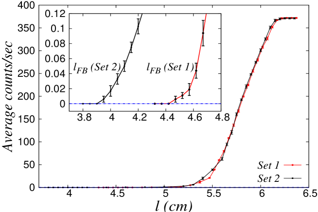
Figure 2: Average count rate (s^-1) as a function of $l$ at the flow rate of 35.0 cc/min and $d=0.78$ mm for the two sets of experiments. The magnified graph (inset) show the first (jet) breakup points in the two sets of experiments.

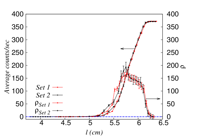
Figure 3: Average count rate (s^-1) and probability distribution as a function of $l$ at the flow rate of 35.0 cc/min and $d=0.78$ mm for the two sets of experiments. The distribution, $\rho$, of breakup length is calculated as the derivative of the count rate with respect to $l$ and the normalized distribution $\rho_{n}$ = $\rho$/100.

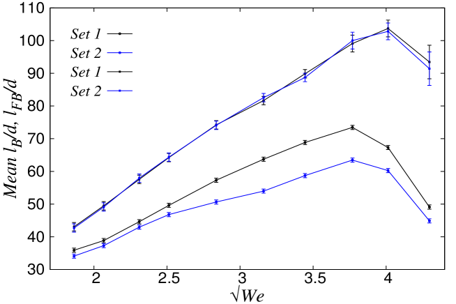
Figure 4: The first breakup length $l_{FB}/d$ (lower set of two curves) and the mean breakup length $l_{B}/d$ (upper set of two curves) as a function of $\sqrt{We}$ for $d=0.78$ mm.

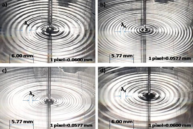
Figure 5: Photograph of the water surface in the beaker for $d=0.95$ mm and water flow rate of 40.0 cc/min. When the jet-length a)$L=0.168$ cm; b) $L=0.568$ cm; c) $L=3.668$ cm; and d) $L=4.268$ cm. The average wavelength ($\lambda_{s}$) on the water surface just appear at a) then decrease with $L$ b) and c) and then increase till it reaches d) (i.e., just before the jet breaks into droplet).

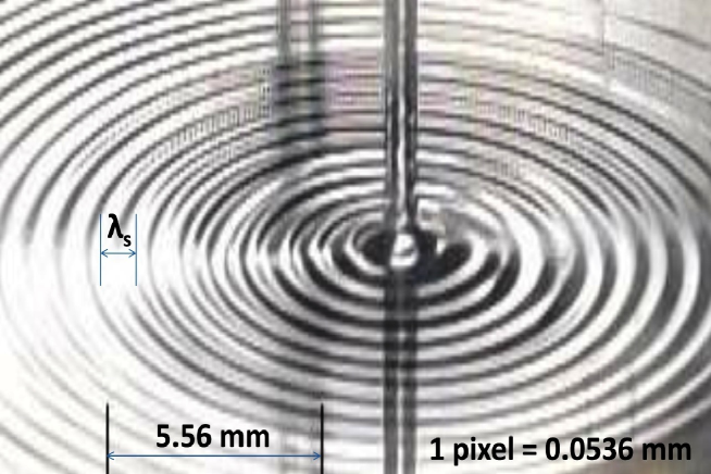
Figure 6: Photograph of the water surface in the beaker when the jet-length $L=0.942$ cm for $d=0.95$ mm and water flow rate of 50.0 cc/min.

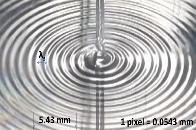
Figure 7: Photograph of the water surface in the beaker when the jet-length $L=1.295$ cm for $d=1.26$ mm and water flow rate of 72.5 cc/min.

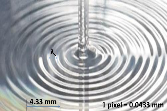
Figure 8: Photograph of the water surface in the beaker when the jet-length $L=1.806$ cm for $d=1.54$ mm and water flow rate of 120.0 cc/min.

All the measurements are done at the temperature of (25$\pm$.5)^∘C and at relative humidity of (80$\pm$4)%. However, in order to calculate the Reynolds number Re ($=\frac{\rho_{w}ud}{\mu}$) and the Weber number We ($=\frac{\rho_{w}u^{2}}{\sigma}\frac{d}{2}$) we have used the tabulated values of surface tension $\sigma=72\times 10^{-3}$ Nm^-1, coefficient of dynamic viscosity $\mu=8.9\times 10^{-4}$ kgm^-1s^-1 and density $\rho_{w}=997.05$ kgm^-3 of water. The issuing jet speed $u$ is calculated as the ratio of the flow rate and the inner area of the nozzle exit.

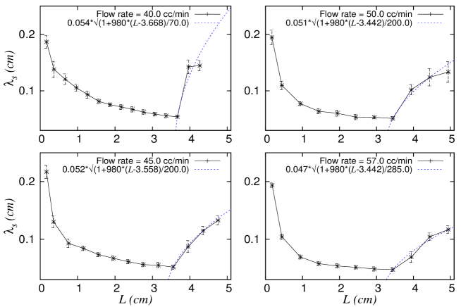
Figure 9: Average wavelength ($\lambda_{s}$) on the water surface of deep water gravity waves as a function of $L$ for d= 0.95 mm.

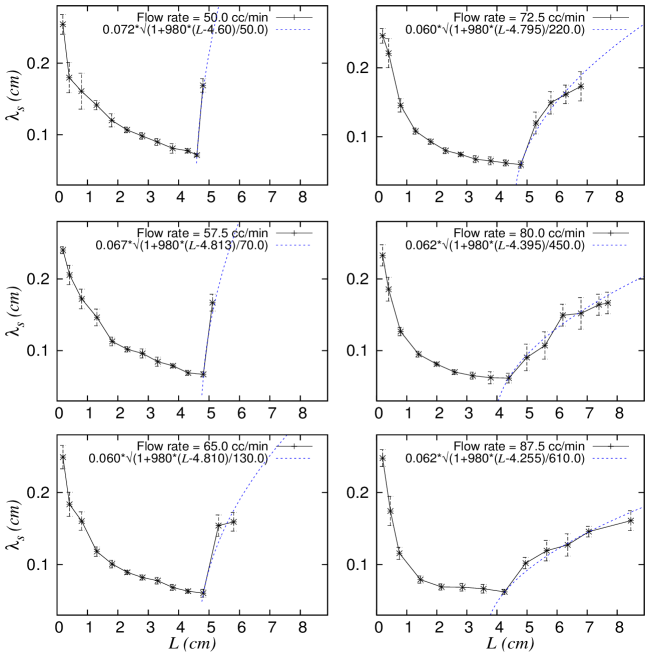
Figure 10: Average wavelength ($\lambda_{s}$) on the water surface of deep water gravity waves as a function of $L$ for d= 1.26 mm.

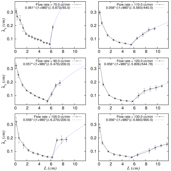
Figure 11: Average wavelength ($\lambda_{s}$) on the water surface of deep water gravity waves as a function of $L$ for d= 1.54 mm.

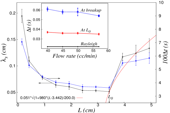
Figure 12: Average wavelength ($\lambda_{s}$) on the water surface and time period ($\Delta$t) of deep water gravity waves as a function of $L$ for d= 0.95 mm and water flow rate of 50.0 cc/min. A numerical fit to $\lambda_{s}$ (for $L>L_{0}$) is also shown.

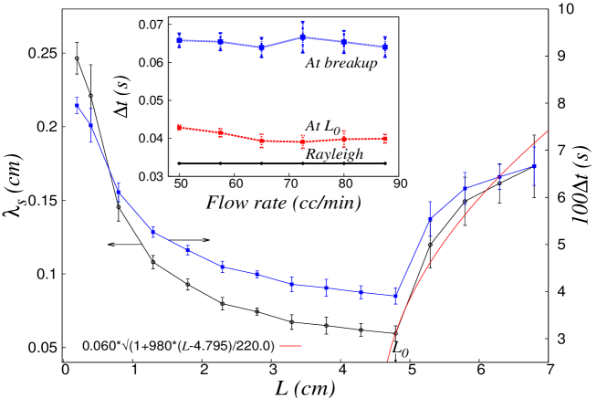
Figure 13: Average wavelength ($\lambda_{s}$) on the water surface and time period ($\Delta$t) of deep water gravity waves as a function of $L$ for d= 1.26 mm and water flow rate of 72.5 cc/min. A numerical fit to $\lambda_{s}$ (for $L>L_{0}$) is also shown.

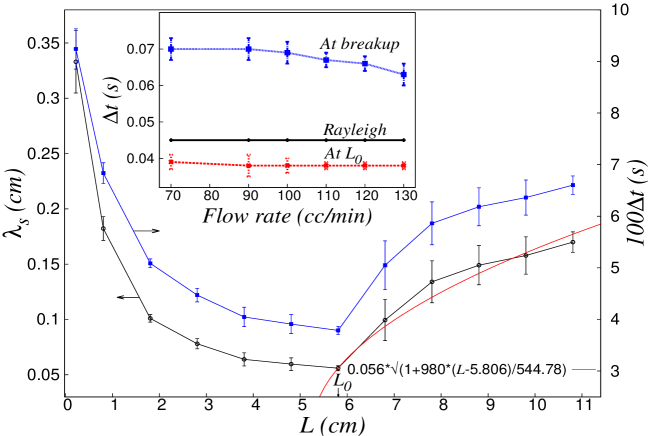
Figure 14: Average wavelength ($\lambda_{s}$) on the water surface and time period ($\Delta$t) of deep water gravity waves as a function of $L$ for d= 1.54 mm and water flow rate of 120.0 cc/min. A numerical fit to $\lambda_{s}$ (for $L>L_{0}$) is also shown.

Figure 2 shows the average number of counts (drops) per second, for a water flow rate of 35.0 cc/min and the nozzle inner diameter $d=0.78$ mm, as a function of jet-length $l$. The counts range from zero to a saturation value and $l_{B}$ are essentially distributed over a range of values due to the absence of any fixed external perturbation and presence of unavoidable noise in the laboratory as remarked by Donnelly et al Donnelly . The mean break-up length is thus calculated using the distribution of breakup lengths $l_{B}$ and it is plotted in Fig. 3.

The magnified picture of the graph for low values of count rates is shown in the inset of Fig. 2. The inset clearly shows that $l_{FB}$ as measured in the first set of experiments is larger by about 5 mm compared to $l_{FB}$ measured in the second set of experiments. Recall that in the first case the recoil capillary wave is damped whereas in the latter case it propagates freely up the jet length. The delay in the process of first breakup of the jet in the first set of experiments indicates that the effect of recoil capillary waves do exist. Or, equivalently, it shows that the tension of the water surface drags the jet down by about 5 mm before it allows the contact between them to breakup. Obviously, the effect of recoil capillary wave is small and its mere absence cannot delay the breakup indefinitely.

In Fig. 4 the mean $l_{B}$ and the $l_{FB}$ for the two sets of experiment are plotted as a function of water flow rate (or, equivalently, as a function of $\sqrt{We}$) for a nozzle of inner diameter 0.78 mm. The difference between $l_{FB}$ for the two sets persists for all flow rates. The experiment was repeated for various other nozzles with internal diameters, d= 0.69 mm,0.72 mm, 0.82 mm, 0.95 mm, 1.04 mm, 1.14 mm, 1.26 mm, 1.34 mm and 1.54 mm. In all cases the results are consistently similar to Fig. 4 and we arrive at the same conclusion about the existence of recoil capillary waves.

As mentioned earlier, Savart’s pioneering experiment together with the Plateau-Rayleigh theory stimulated further investigations on surface profile of the jet and its breakup, for exampleDonnelly ; Rutland . We capture the waves produced on the surface of the water in the beaker photographically as the continuous water jet merges into the water body. Figure 5 shows a sequence of photographs at different $L=0.168,~{}0.568,~{}3.668$, and $4.268$ cms, respectively, for nozzle diameter $d=0.95$ mm and a flow rate of $FR=$40 cc/min. Similar photpgraphs can be obtained for other nozzle diameters ($d$) flow rates $FR$ at different jet length $L$ as well. Figures 6-8 show representative photographs for $d=0.95$ mm and $FR=50$ cc/min at $L=0.942$ cm, $d=1.26$ mm, $FR=72.5$ cc/min at $L=1.295$ cm, and $d=1.54$ mm, $FR=120.0$ cc/min at $L=1.806$ cm, respectively.

We contend that the waves are produced on the water surface due to the time periodic variation of cross-section of the jet, that is, due to the periodic crossings of necks and bulges of the jet, at the position of the water surface. We vary $L$ from zero till the jet-breakup becomes imminent and take phographs of the water surface for various $L$. We find that no waves are produced on the water surface when $L$ was zero. On increasing $L$ we could discern the appearance of the circular waves for the first time when $L$ was 0.221 cm for $d=1.54$ mm and $FR=120.0$ cc/min. As we gradually lower the water surface the circular waves become sharper and then on further increasing $L$ the surface waves begin to wane. At a particular $L=L_{0}$ the waves become the least sharp. However, on further lowering the surface, the waves reappear with increased sharpness and the waves persist till ultimately the jet breaks up before touching the water surface. Figure 5 exhibits the above mentioned behavior for nozzle diameter $d=0.95$ mm and a flow rate of $FR=$40 cc/min. Similar behavior is also observed for other nozzle diameters ($d$) flow rates $FR$ at different jet length $L$ as well.

We measure the wavelengths $\lambda_{s}$ of the waves on the water surface using the photographs. Figures 9-11 show the measured wavelengths ($\lambda_{s}$) as a function of $L$, respectively, for $d=0.95,~{}1.26$ and 1.54 mm. The length scales of the waves are much smaller than the depth ($\approx$ 6 cm) of the water in the beaker. Thus these waves can be considered as deep water gravity waves. From the measured $\lambda_{s}$ we calculate the group velocities $v_{g}=\sqrt{\frac{g_{0}\lambda_{s}}{8\pi}}$ of these waves, where the acceleration due to gravity $g_{0}$=9.8 m/s². From these data we calculate the time difference ($\Delta t$) between two consecutive crests of the waves. The $\Delta t(\propto\sqrt{\lambda}_{s})$, are also plotted in Figs. 12-14 together with $\lambda_{s}$, for the same $d$ values as in Figs. 9-11. This $\Delta t$ can also be taken as the time difference between two bulges of the jet ’hitting’ the water surface.

The measured $\lambda_{s}$ initially decreases as $L$ increases and reaches a minimum value at $L=L_{0}$ and thereafter, the $\lambda_{s}$ increases with $L$. $L=L_{0}$ thus marks a sharp boundary in the nature of the water jets. We conjecture that the minimum $\lambda_{s}$ corresponds to the fastest growing Rayleigh perturbation in the jet and not the one at the breakup point $L=l_{B}$. This is partially supported by roughly similar values of $\Delta t$. For instance, in the inset of Fig. 14, $\Delta t\approx 0.038$ s at the minimum of $\lambda_{s}$ (at $L=L_{0}$) is roughly equal to the time scale $\tau=\frac{2\pi}{\omega}\approx 0.045$ s obtained from the estimate of the frequency $\omega$ at the maximum of the dispersion curve of the Plateau-Rayleigh theory and measured by Goedde and Yuen, (Fig. 7 of Ref.Goedde ). Moreover, the $\Delta t$ at the breakup point ($L=l_{B}$) of the jet is comparatively far different from $\tau=0.045$.

The competition between various modes of Rayleigh perturbations makes the jet-surface profile variation dynamic before $\lambda_{s}$ becomes a minimum. In other words, the jet-surface profile changes along the length ($L<L_{0}$) of the jet satisfying the stability conditions of Rayleigh theory and affected very little by gravity. This is the only way we can explain the variation of $\Delta t$, for example in Fig. 14, from about 0.09s to 0.04s keeping the constancy of mean mass flow rate of water at any section of the jet.

We contend that for $L<L_{0}$, the effect of surface tension dominates over the gravitational effect on the jet whereas at larger $L>L_{0}$ the gravitational effect plays a dominant role making the surface profile of the jet nonsinusoidal. The nonsinusoidal surface profile can also be seen from the high speed photographs of Ref.Rutland .

In the spirit of Ref.Scriven , and considering $\lambda_{s}$ to be proportional to the difference in jet length between two bulgings, we numerically fit $\lambda_{s}(L)$ of the waves on the water surface of the beaker (Figs. 9-14) as $\lambda_{s}(L)=\lambda_{s}(L_{0})\sqrt{1+\frac{2g_{0}(L-L_{0})}{u_{0}^{2}}}$ taking $u_{0}$ as a fitting parameter. As can be seen the fit is reasonable. We could similarly fit the data for all other nozzles in a range of flow rates. Our contention of dominance of gravitational effect for $L>L_{0}$ thus has good experimental support.

IV Conclusion

In conclusion, our experiment verifies the existence of recoil capillary waves and its effect on jet breakup and points out the relative importance of Rayleigh perturbations and gravitational effects on the jet surface profile. The photographs of surface waves created by the jets on the water surface helps us measure the wavelegths of the surface waves. The behavior of the surface wave lengths show a sharp transition as a function of the jet length. The jet length $L_{0}$ at the transition point is different for different nozzle diameters and flow rates. For $L<L_{0}$ Rayleigh perturbations dominate whereas for $L>L_{0}$ gravitaional effect is more important.

References

- (1) J. Eggers, Rev. Mod. Phys. 69, 865 (1997).
- (2) J. Eggers, and E. Villermaux, Rep. Prog. Phys. 71, 036601 (2008).
- (3) S. P. Lin, Breakup of Liquid Sheets and Jets, Cambridge University Press, 2010.
- (4) B. Lautrup, Physics of Continuous Matter, Second Edition, CRC Press, Boca Raton, 2011.
- (5) Lord, J. W. S. Rayleigh, Proc. London Math. Soc. 10, 4 (1879).
- (6) J. W. S. Rayleigh, The Theory of Sound, Vol. II, pp. 351-375, Dover Publications, New York, 1945.
- (7) S. Chandrasekhar, Hydrodynamic and Hydromagnetic Stability, Dover Publications, New York, 1961.
- (8) E. F. Goedde, and M. C. Yuen, J. Fluid Mech. 40, 495 (1970).
- (9) A. Umemura, Phys. Rev. E 83, 046307 (2011).
- (10) A. Umemura, S. Kawanabe, S. Suzuki, and J. Osaka, Phys. Rev. E 84, 036309 (2011).
- (11) A. Umemura, and J. Osaka, J. Fluid Mech. 752, 184 (2014).
- (12) A. Umemura, J. Fluid Mech. 575, 665 (2014); ibid 797, 146 (2016).
- (13) W. K. Bani, and M. C. Mahato, arXiv:1608.04915v1 [physics.flu-dyn].
- (14) We have used a (3.5-4.99 mW) Taurus Series 635 nm (Class IIIa) red laser pointer, a photoconductive LDR (1K) sensor (detector), a UA741CN Op Amp, a SN74LS14N Hex Inverter Schmidt Trigger, a 74ALS04BN Hex Inverter, HCF4033BEs and CD4026BEs decade counters, a NE555P timer, HEF4082BPs AND Gate, Common Cathode 7-Segment single digit LED display in the experimental set up.
- (15) R. J. Donnelly, and W. Glaberson, Proc. Roy. Soc. A 290, 547(1966).
- (16) D. F. Rutland, and G. J. Jameson, J. Fluid Mech. 46, 267 (1971).
- (17) L. E. Scriven, and R. L. Pigford, A.I.Ch.E Journal 5, 397(1959).