Diagonal Slice Four-Wave Mixing: Natural Separation of Coherent Broadening Mechanisms

Abstract

We present an ultrafast coherent spectroscopy data acquisition scheme that samples slices of the time domain used in multidimensional coherent spectroscopy to achieve faster data collection than full spectra. We derive analytical expressions for resonance lineshapes using this technique that completely separate homogeneous and inhomogeneous broadening contributions into separate projected lineshapes for arbitrary inhomogeneous broadening. These lineshape expressions are also valid for slices taken from full multidimensional spectra and allow direct measurement of the parameters contributing to the lineshapes in those spectra as well as our own.

Multidimensional Coherent Spectroscopy (MDCS) is a powerful spectroscopic tool for measuring dephasing and coherent dynamics of electronic and vibrational resonances on ultrafast timescales [1, 2, 3, 4, 5]. MDCS was first implemented in nuclear magnetic resonance (NMR) experiments using radio frequencies [6, 7, 8, 9], was then used to study vibrational coupling in the IR [10], and has recently been extended to electronic resonances in the visible and phonons in solids at terahertz frequencies [11, 12, 13].

An advantange of MDCS is that the coupling between resonances becomes obvious and seperable because they are spread across multiple frequency dimensions; a result not available in linear spectroscopy. Because of this, MDCS provides a clear visualization of the qualitative dynamics of the system and rich quantitative information on material properties that are accessible through analysis of the resonance lineshapes present in the spectra. For example, homogeneous and inhomogeneous mechanisms broaden the resonance in orthogonal directions in a MDCS spectrum, allowing straightforward separation and identification of these contributions [14].

While powerful and intuitive, it is difficult to quantify material properties due to the increased complexity of multidimensional lineshapes. One dimensional lineshape analysis has historically enabled measurement of the oscillator strength [15], excitation lifetime [16, 17], homogeneous and inhomogeneous linewidths [18, 19, 20], and chemical shifts [21]. The most common approach to optical multidimensional data sets employs quasi one-dimensional lineshape analysis of frequency-domain slices [22], although other approaches exist [23, 24, 25]. That method required taking data slices from the frequency domain for lineshape fitting. The frequency slice approach can be used to measure changes in the homogeneous response of an inhomogeneous distribution [26, 27, 14]. However, all extracted slices depend on both homogeneous and inhomogeneous broadening. This problem can be mitigated by simultaneous fitting of diagonal and cross-diagonal lineshapes or fitting entire MDCS spectra [22, 23]. However, to our knowledge, no MDCS lineshape analysis has completely separated homogeneous and inhomogeneous broadening.

In this letter, we present diagonal slice four-wave mixing (DS-FWM), a data acquisition scheme for rapidly measuring material properties accessible in a MDCS spectrum without acquiring a full MDCS data set.

Critically, our analysis determines both a time-domain basis and frequency-domain analytic functions that are orthogonal with respect to the broadening mechanisms found in MDCS by utilizing time slices from the rephasing pulse sequence in either the diagonal or cross-diagonal directions. We derive analytical expressions for the complex signal response in which different broadening mechanisms are decoupled along different time axes, using perturbative solutions to the optical Bloch equations (OBEs). Analytical expressions for frequency domain projections are derived by applying the projection-slice theorem to the time-domain slices. The resulting frequency-domain expressions completely separate the homogeneous and inhomogeneous broadening, fit simulated resonances and experimental data from GaAs quantum wells (QWs), and demonstrate excellent agreement with previously used lineshape analysis.

The Projection-Slice Theorem states that the Fourier transform of a slice in two dimensions is equivalent to a projection onto that axis in the Fourier domain [24]. Mathematically,

$$P(k_{x})=\mathcal{F}[S(x)]=\int_{-\infty}^{\infty}S(x)e^{-i2\pi k_{x}x}dx,$$ (1)

where $S(x)$ denotes a slice in any arbitrary $x$ direction and $P(k_{x})$ denotes a projection onto the same $k_{x}$ axis in the Fourier domain. We consider only the rephasing pulse sequence for a sample with inhomogeneous broadening. This system will exhibit a photon-echo at $t=\tau$, where $\tau,\,T=0,\,t$ are the inter-pulse delays between the first-second ($\tau$), second-third ($T$), and third-fourth ($t$) pulses. Note, in the present analysis the signal is assumed to be a third order coherence mapped onto a fourth order population by a fourth pulse in contrast to heterodyning schemes [28, 29].

The perturbative time-domain solution to the OBEs for an inhomogeneously broadened ensemble of two-level systems interacting with this pulse sequence is;

$$s(t,\tau)=s_{0,0}e^{-\left(\gamma\left(t+\tau\right)+i\omega_{0}\left(t-\tau\right)+\sigma^{2}\left(t-\tau\right)^{2}/2\right)}\Theta(t)\Theta(\tau),$$ (2)

where $s_{0,0}$ is the signal amplitude at time zero, $\omega_{0}$ is the center frequency of the resonance, $\gamma$ and $\sigma$ are the homogeneous and inhomogeneous dephasing rates, $\Theta$ denotes a unit step function that enforces causality between the pulses and the signal, and $\tau$ ($t$) is the time delay corresponding to absorption (emission) processes. In the frequency domain, $\omega_{\tau}$ ($\omega_{t}$) is the frequency axis for absorption (emission) processes. Recent work has extended the formalism of spectral analysis to include non-delta function pulses [30], pulses with chirp [31], and non-Gaussian responses [32]. However, in this study these considerations are excluded in that delta function pulses and Gaussian inhomogeneous broadening are assumed.

We can now rewrite Eq. (1) in terms of physical parameters relevant to MDCS data,

$$P(\omega_{t}+\omega_{\tau})=\int_{-\infty}^{\infty}S(t+\tau)e^{i2\pi(t+\tau)(\omega_{t}+\omega_{\tau})}d(t+\tau).$$ (3)

The two orthogonal time axes $t^{\prime}=\frac{\left(t+\tau\right)}{\sqrt[]{2}}$ and $\tau^{\prime}=\frac{\left(t-\tau\right)}{\sqrt[]{2}}$ (shown in Fig. 1) correspond to the diagonal and cross-diagonal directions in the MDCS time domain, and allow Eq. 2 to be rewritten in this new basis. The signal normalized to $s_{0,0}$ in this new basis is

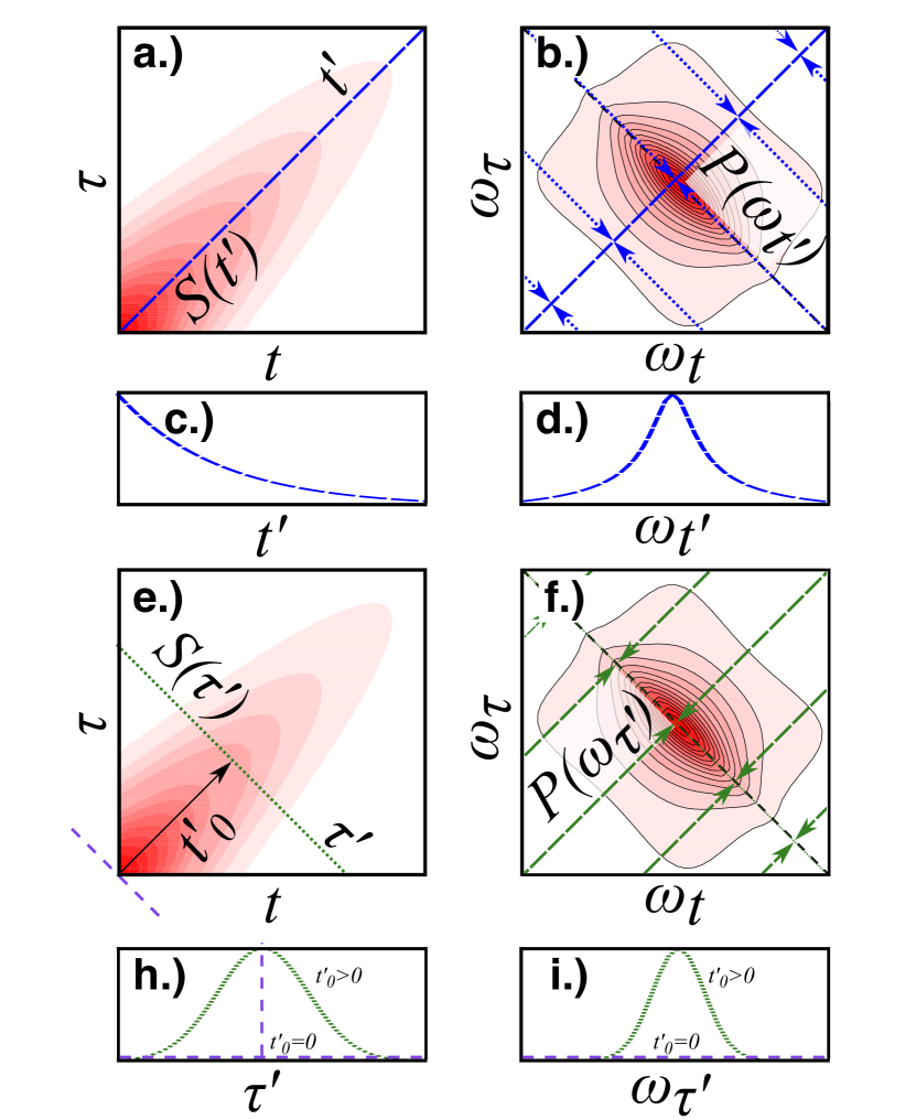
Figure 1: Diagram showing the rotated coordinate system in the MDCS time [a.), e.)] and frequency domains [b.), f.)], along with the slices [c.), h.)], and associated projections [d.), i.)], that are the focus of this work. The dashed lines in a.) and e.) represent the data slices in the time domain and arrow tipped lines in b.) and f.) represent bins that are integrated in the projections. All plots show the simulated rephasing amplitude.

$$s(t^{\prime},\tau^{\prime})=e^{-\left(\sqrt[]{2}\gamma t^{\prime}+\,i\,\,\sqrt[]{2}\omega_{0}\tau^{\prime}+\,\sigma^{2}\tau^{\prime 2}\right)}\Theta(t^{\prime}-\tau^{\prime})\Theta(t^{\prime}+\tau^{\prime}).$$ (4)

This form of the signal simplifies the contribution of homogeneous and inhomogeneous broadening to the diagonal ($t^{\prime}$) and cross-diagonal ($\tau^{\prime}$) linewidths, at the cost of adding complexity to the step functions involved.

The Fourier transform of time domain slices provides simplified expressions in both the time and frequency domains.

A slice along $t^{\prime}$, at $\tau^{\prime}=0$, gives

$$S(t^{\prime},\tau^{\prime}=0)=e^{-\sqrt[]{2}\gamma t^{\prime}}\Theta^{2}(t^{\prime})$$ (5)

and a slice along $\tau^{\prime}$, at a fixed $t^{\prime}=t^{\prime}_{0}$, results in the expression

$$s(t^{\prime}=t_{0}^{\prime},\tau^{\prime})=e^{-\left(\sqrt[]{2}\gamma t_{0}^{\prime}+i\,\,\sqrt[]{2}\omega_{0}\tau^{\prime}+\sigma^{2}\tau^{\prime 2}\right)}\Theta(t_{0}^{\prime}-\tau^{\prime})\Theta(t_{0}^{\prime}+\tau^{\prime}),$$ (6)

where $t^{\prime}_{0}$ is the intercept of the slice on the $t^{\prime}$ axis. We note here that $t^{\prime}_{0}$ must be greater than zero to retrieve any meaningful information from a dataset that does not extend to negative delays. As shown by the purple dashed line in Fig. 1 [e.), h.), i.)], a slice along $t^{\prime}_{0}=0$ gives a delta function in time that when Fourier transformed becomes a constant in the frequency domain. Likewise, a slice at $t^{\prime}_{0}<0$ will be zero everywhere due to the step functions enforcing causality.

Fourier transforming Eq. 5 gives

$$P(\omega_{t^{\prime}})=\frac{1}{\sqrt[]{2\pi}\left(\sqrt[]{2}\gamma-i\omega_{t^{\prime}}\right)},$$ (7)

with an absorptive (dispersive) Lorentzian component for the real (imaginary) part of the lineshape. The absolute value of this complex lineshape is a square root Lorentzian, with a full-width at half-maximum (FWHM) of $\sqrt[]{2}\gamma$. The Fourier transform of the $\tau^{\prime}$ slice gives

$$P(\omega_{\tau^{\prime}}) =e^{-\sqrt[]{2}t_{0}^{\prime}\gamma}\,\,\frac{e^{-\left(\frac{\sqrt[]{2}\omega_{0}-\omega_{\tau^{\prime}}}{2\sigma}\right)^{2}}}{4\sigma}$$ (8)

$$\bigg{(}Erf\left[t_{0}^{\prime}\sigma+\frac{i\left(\sqrt[]{2}\omega_{0}-\omega_{\tau^{\prime}}\right)}{2\sigma}\right]$$

$$+Erf\left[t_{0}^{\prime}\sigma-\frac{i\left(\sqrt[]{2}\omega_{0}-\omega_{\tau^{\prime}}\right)}{2\sigma}\right]\bigg{)}$$

which does have a $\gamma$ dependent term, but only as a constant scaling factor that does not affect the lineshape. Here $Erf$ denotes an error function. The expression in Eq. 8 has a Gaussian lineshape with a FWHM of $4\,\,\sqrt[]{ln\left(2\right)}\sigma$.

The expressions in Eqs. 7 and 8 are analytical projections onto the $\omega_{t^{\prime}}$ and $\omega_{\tau^{\prime}}$ axes, respectively. The use of the projection-slice theorem to arrive at these expressions is similar to the treatment of NMR spectra in [24] with the important distinction that we use only the $t^{\prime}$ and $\tau^{\prime}$ directions to take advantage of their isolated $\gamma$ and $\sigma$ dependent behavior.

These expressions show the advantage of using the frequency projection as the basis for lineshape analysis: complete separation of the inhomogeneous and homogeneous broadening via their independent axes. These expressions thus improve upon previous analysis [22, 23] that resulted in coupled expressions for the different broadening mechanisms.

The disadvantage of DS-FWM is that taking a projection removes the individual information content providing only an average material response [33]. Thus projections onto the frequency axis may be a more natural basis for considering single resonances or ensemble responses as a whole, while slices along the frequency axis are better suited to studying the response of individual oscillators in an ensemble.

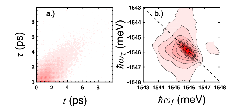
Figure 2: Experimental MDCS data from GaAs QWs in the a.) Time and b.) frequency domain corresponding to the DS-FWM data shown in Figs. 3 and 4. Both spectra are absolute value rephasing spectra.

To validate the derived expressions we use them to fit simulated and experimental data. The experimental setup used is described in [34, 35], with the signal collected via photoluminescence (PL). This signal choice provides a direct analog to optical Ramsey spectroscopy in atomic physics. Briefly, a pulsed Ti:Sapphire oscillator (Spectra-Physics Tsunami), with $90\,fs$ pulses and a bandwidth of $30\,meV$ is split into four identical copies, each with a precisely controlled delay via mechanical translation stages. Each beam is passed through an acousto-optic modulator (AOM) (Isomet 1205-C) where it is given a unique carrier frequency shift with a distinct radio frequency (RF). The resulting pulse train undergoes dynamic, pulse to pulse, phase cycling that averages out unwanted signal contributions and forces the signal PL to beat at RF frequencies specific to the desired quantum pathway.

This signal choice requires that all data must be collected in the time domain, point by point. This can significantly increase the number of points, and hence the acquisition time to acquire a MDCS spectrum as compared to measurements using a spectrometer. However, by only collecting data along the $t^{\prime}$ and $\tau^{\prime}$ directions, we can measure the homogeneous and inhomogeneous linewidths in a similar amount of time that a coherently detected MDCS experiment could with no ambiguity or mixing of the broadening contributions. DS-FWM provides a greatly simplified analysis to extract many of the most important physical parameters accessible with MDCS. We realize data collection along the $t^{\prime}$ and $\tau^{\prime}$ axes by simultaneously stepping the stages that control $t$ and $\tau$ time delays in our experiment and collecting data at each point. This treatment is similar to the radial sampling used in some NMR experiments to reduce data collection time [36], with the difference that we do not reconstruct full MDCS datasets from our projections.

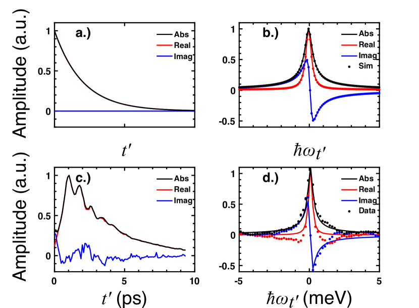
Figure 3: Time [a.), c.)] and frequency [b.), d.)] domain DS-FWM data for a simulated resonance [a.), b.)] and GaAs QWs [c.), d.)]. All data was taken in the $\tau^{\prime}$ direction and fit using Eq. 7. Dots show the data and solid lines show the function with best fit parameters $\left(\gamma=0.1051\,meV\right)$.

To verify the derived DS-FWM expressions, we fit both simulated and experimental data to our complex functions. The sample used in this experiment consists of four $GaAs$ QWs surrounded by $Al_{0.3}Ga_{0.7}As$ barriers. It has been previously shown that strained bulk $GaAs$ [37] and ’natural quantum dots’ [38] can be present in QW samples, in addition to the light hole (LH) exciton that is present in the sample. Here, we isolate the resonance of the heavy-hole (HH) exciton in the well by checking its frequency in a PL spectrum (Ocean Optics USB2000) and tuning the excitation frequency to the HH PL frequency, with as little overlap with the LH exciton as possible. The sample is kept at a temperature below 10K by a recirculating liquid Helium cryostat (Montana Instruments Cryostation). For simulated data of a single resonance with $\frac{\sigma}{\gamma}\approx 3$, both the diagonal, and cross-diagonal, projection is fit with $r^{2}\approx.9999$. We then took DS-FWM spectra, in both the $t^{\prime}$ and $\tau^{\prime}$ directions. The experimental $\omega_{t^{\prime}}$ projection was fit to our expressions with $r^{2}\approx.9682$ and the $\omega_{\tau^{\prime}}$ projections fit the data with $r^{2}\approx 0.9718$. The results of these fits can be seen in Figs. 3 and 4. We acknowledge that the sample system was not the ideal single resonance assumed by the derivation, as can clearly be seen in the beating of the GaAs QW time-domain data in Figs. 2 and 3. The LH exciton of the quantum well has a small signal that is present in the DS-FWM spectra but is much weaker than the HH resonance and should not significantly contribute to the projected lineshapes. Furthermore, we note that we have normalized the amplitude of our projections to unity in our treatment of the data. Normalizing the data in this way forfeits our ability to extract oscillator strengths from our fits, as we are focused on the broadening contributions of the resonance.

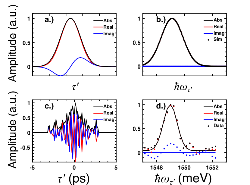
Figure 4: Time [a.), c.)] and frequency [b.), d.)] domain DS-FWM data for a simulated resonance [a.), b.)] and GaAs QWs [c.), d.)]. All data was taken in the $\tau^{\prime}$ direction and fit using Eq. 7. Dots show the data and solid lines show the function with best fit parameters $\left(\omega_{0}=1548.97,\,\sigma=0.306\,meV\right)$.

We note that this procedure may be performed directly by the experiment in the time domain by only collecting data in the $t^{\prime}$ and $\tau^{\prime}$ directions or in the analysis of a full MDCS spectrum by extracting data slices from a larger data set. We have performed our analysis using each of these procedures and seen no significant difference in the results. We also note that any MDCS experiment that collects all data in the time domain, such as those that detect a population with a fourth readout pulse as opposed to an emitted electric field or those that use a fourth pulse for heterodyne detection on a photodiode, is already set up to take DS-FWM spectra, although the potential of a simplified experimental setup that collects data slices only along $t^{\prime}$ and $\tau^{\prime}$ in the MDCS time domain is very promising. Such an experiment could access critically relevant material parameters $\left(\gamma,\sigma,\omega_{0}\right)$ without the data collection times and experimental complexity of many MDCS experiments.

In this letter, we have presented a data collection scheme for ultrafast coherent spectroscopy and an associated lineshape analysis that is applicable to MDCS spectra as well as DS-FWM spectra. We have derived analytical expressions for slices along the $t^{\prime}$ and $\tau^{\prime}$ axes in the MDCS time domain, as well as expressions for the associated frequency domain $\omega_{t^{\prime}}$ and $\omega_{\tau^{\prime}}$ projections and shown that these projections completely separate the homogeneous and inhomogeneous broadening mechanisms to the lineshape. We have fit these expressions to both simulated and experimental data and shown excellent agreement. The technique presented here offers a deeper insight into the nature of lineshape broadening in coherent spectroscopy as well as a protocol for faster data collection to find key material parameters.

National Science Foundation (NSF) (1511199, 1553905).

The authors thank Christopher Smallwood and Matthew Day for advice on photoluminescence detection and for sharing their design of a custom amplifier circuit, as well as Samuel Alperin and Jasmine Knudsen for helpful discussions concerning the manuscript. T.M.A. acknowledges support from a National Research Council (NRC) Research Associate Program (RAP) award at the National Institute of Standards and Technology (NIST).

© 2018 Optical Society of America. Users may use, reuse, and build upon the article, or use the article for text or data mining, so long as such uses are for non-commercial purposes and appropriate attribution is maintained. All other rights are reserved.

References

- [1] Steven T Cundiff. Coherent spectroscopy of semiconductors. Optics Express, 16(7):4639, 2008.
- [2] David M. Jonas. Two Dimensional Femtosecond Spectroscopy. Annual Review of Physical Chemistry, 54(1):425–463, 2003.
- [3] Minhaeng Cho. Coherent two-dimensional optical spectroscopy. Chem. Rev., 108(4):1331–1418, 2008.
- [4] Gaël Nardin. Multidimensional coherent optical spectroscopy of semiconductor nanostructures: a review. Semiconductor Science and Technology, 31(2):023001, 2016.
- [5] Robert W. Boyd. Nonlinear Optics. Book, page 613, 2008.
- [6] W. P. Aue, E. Bartholdi, and R. R. Ernst. Two-dimensional spectroscopy. Application to nuclear magnetic resonance. The Journal of Chemical Physics, 64(5):2229–2246, 1976.
- [7] J. Jeener, B. H. Meier, P. Bachmann, and R. R. Ernst. Investigation of exchange processes by two-dimensional NMR spectroscopy. The Journal of Chemical Physics, 71(11):4546–4553, 1979.
- [8] Richard R. Ernst, Geoffrey Bodenhausen, and Alexander Wokaun. Principles of Nuclear Magnetic Resonance in One and Two Dimensions. Clarendon, New York, 1987.
- [9] Richard Ernst. Richard Ernst Nobel Lecture - NMR Spectroscopy.
- [10] Peter Hamm, Manho Lim, and Robin M. Hochstrasser. Structure of the Amide I Band of Peptides Measured by Femtosecond Nonlinear-Infrared Spectroscopy. The Journal of Physical Chemistry B, 102(31):6123–6138, 1998.
- [11] John D. Hybl, Allison W. Albrecht, Sarah M. Gallagher Faeder, and David M. Jonas. Two-dimensional electronic spectroscopy. Chemical Physics Letters, 297(3-4):307–313, 1998.
- [12] W. Kuehn, K. Reimann, M. Woerner, T. Elsaesser, R. Hey, and U. Schade. Strong correlation of electronic and lattice excitations in GaAs/AlGaAs semiconductor quantum wells revealed by two-dimensional terahertz spectroscopy. Physical Review Letters, 107(6):2–6, 2011.
- [13] W. Kuehn, K. Reimann, M. Woerner, and T. Elsaesser. Phase-resolved two-dimensional spectroscopy based on collinear n -wave mixing in the ultrafast time domain. Journal of Chemical Physics, 130(16), 2009.
- [14] Alan D. Bristow, Tianhao Zhang, Mark E. Siemens, Steven T. Cundiff, and R. P. Mirin. Separating homogeneous and inhomogeneous line widths of heavy- and light-hole excitons in weakly disordered semiconductor quantum wells. Journal of Physical Chemistry B, 115(18):5365–5371, 2011.
- [15] M. V. Belousov, N. N. Ledentsov, M. V. Maximov, P. D. Wang, I. N. Yasievich, N. N. Faleev, I. A. Kozin, V. M. Ustinov, P. S. Kop’ev, and C. M. Sotomayor Torres. Energy levels and exciton oscillator strength in submonolayer InAs-GaAs heterostructures. Physical Review B, 51(20):14346–14351, 1995.
- [16] R. P. Stanley, J. Hegarty, R. Fischer, J. Feldmann, E. O. Göbel, R. D. Feldman, and R. F. Austin. Hot-exciton relaxation in CdxZn1-xTe/ZnTe multiple quantum wells. Physical Review Letters, 67(1):128–131, 1991.
- [17] M. Wegener, D. S. Chemla, S. Schmitt-Rink, and W. Schäfer. Line shape of time-resolved four-wave mixing. Physical Review A, 42(9):5675–5683, 1990.
- [18] G. Noll, U. Siegner, S. G. Shevel, and E. O. Göbel. Picosecond stimulated photon echo due to intrinsic excitations in semiconductor mixed crystals. Physical Review Letters, 64(7):792–795, 1990.
- [19] H. Schwab, V. G. Lyssenko, and J. M. Hvam. Spontaneous photon echo from bound excitons in CdSe. Physical Review B, 44(8):3999–4001, 1991.
- [20] J. Erland, K. H. Pantke, V. Mizeikis, V. G. Lyssenko, and J. M. Hvam. Spectrally resolved four-wave mixing in semiconductors: Influence of inhomogeneous broadening. Physical Review B, 50(20):15047–15055, 1994.
- [21] Steve C F Au-Yeung and Donald R. Eaton. A model for estimating Co nmr chemical shifts and line widths and its application to.pdf. Can. J. Chem, 61(8):2431–2441, 1983.
- [22] Mark E Siemens, Galan Moody, Hebin Li, Alan D Bristow, and Steven T Cundiff. Resonance lineshapes in two-dimensional Fourier transform spectroscopy. Optics express, 18(17):17699–17708, 2010.
- [23] Joshua D Bell, Rebecca Conrad, and Mark E Siemens. Analytical calculation of two-dimensional spectra. Optics Letters, 40(7):1157, 2015.
- [24] K. Nagayama, P. Bachmann, K. Wuthrich, and R. R. Ernst. The use of cross-sections and of projections in two-dimensional NMR spectroscopy. Journal of Magnetic Resonance (1969), 31(1):133–148, 1978.
- [25] Andrei Tokmakoff. Two-dimensional line shapes derived from coherent third-order nonlinear spectroscopy. Journal of Physical Chemistry A, 104(18):4247–4255, 2000.
- [26] Steven T. Cundiff, Alan D. Bristow, Mark Siemens, Hebin Li, Galan Moody, Denis Karaiskaj, Xingcan Dai, and Tianhao Zhang. Optical 2-d fourier transform spectroscopy of excitons in semiconductor nanostructures. IEEE Journal on Selected Topics in Quantum Electronics, 18(1):318–328, 2012.
- [27] Steven T. Cundiff. Optical two-dimensional Fourier transform spectroscopy of semiconductor nanostructures [Invited]. Journal of the Optical Society of America B, 29(2):A69, 2012.
- [28] Eric W. Martin and Steven T. Cundiff. Inducing coherent quantum dot interactions. Physical Review B, 97(8):081301, 2018.
- [29] Ch J. Bordé, Ch Salomon, S. Avrillier, A. Van Lerberghe, Ch Bréant, D. Bassi, and G. Scoles. Optical Ramsey fringes with traveling waves. Physical Review A, 30(4):1836–1848, 1984.
- [30] Christopher Smallwood, Travis Autry, and Steven Cundiff. Analytical solutions to the finite-pulse Bloch model for multidimensional coherent spectroscopy. Journal of the Optical Society of America B, 34(2), 2016.
- [31] Daniel D. Kohler, Blaise J. Thompson, and John C. Wright. Frequency-domain coherent multidimensional spectroscopy when dephasing rivals pulsewidth: Disentangling material and instrument response. Journal of Chemical Physics, 147(8), 2017.
- [32] Marwa H. Farag, Bernhard J. Hoenders, Jasper Knoester, and Thomas L.C. Jansen. Spectral line shapes in linear absorption and two-dimensional spectroscopy with skewed frequency distributions. Journal of Chemical Physics, 146(23), 2017.
- [33] G. Moody, M. E. Siemens, A. D. Bristow, X. Dai, D. Karaiskaj, A. S. Bracker, D. Gammon, and S. T. Cundiff. Exciton-exciton and exciton-phonon interactions in an interfacial GaAs quantum dot ensemble. Physical Review B - Condensed Matter and Materials Physics, 83(11):1–7, 2011.
- [34] Gaël Nardin, Travis M. Autry, Kevin L. Silverman, and S. T. Cundiff. Multidimensional coherent photocurrent spectroscopy of a semiconductor nanostructure. Optics Express, 21(23):28617, 2013.
- [35] Patrick F. Tekavec, Geoffrey A. Lott, and Andrew H. Marcus. Fluorescence-detected two-dimensional electronic coherence spectroscopy by acousto-optic phase modulation. Journal of Chemical Physics, 127(21), 2007.
- [36] Eriks Kupče and Ray Freeman. Fast multidimensional NMR: Radial sampling of evolution space. Journal of Magnetic Resonance, 173(2):317–321, 2005.
- [37] Brian L. Wilmer, Daniel Webber, Joseph M. Ashley, Kimberley C. Hall, and Alan D. Bristow. Role of strain on the coherent properties of GaAs excitons and biexcitons. Physical Review B, 94(7):1–7, 2016.
- [38] G. Moody, M. E. Siemens, A. D. Bristow, X. Dai, A. S. Bracker, D. Gammon, and S. T. Cundiff. Exciton relaxation and coupling dynamics in a GaAs/AlxGa 1-xAs quantum well and quantum dot ensemble. Physical Review B - Condensed Matter and Materials Physics, 83(24):1–7, 2011.