Tsallis holographic dark energy in the brane cosmology

Abstract

We study some cosmological features of Tsallis holographic dark energy (THDE) in Cyclic, DGP and RS II braneworlds. In our setup, a flat FRW universe is considered filled by a pressureless source and THDE with the Hubble radius as the IR cutoff, while there is no interaction between them. Our result shows that although suitable behavior can be obtained for the system parameters such as the deceleration parameter, the models are not always stable during the cosmic evolution at the classical level.

I Introduction

Due to the weakness of general relativity to describe the current accelerated universe Riess ; roos , physicists try to eliminate this difficulty by $i$) introducing amazing energy sources, called dark energy, $ii$) modifying the general relativity theory or even a combination of these. Braneworld scenario is an interesting approach to modify the Einstein theory, and Dvali-Gabadadze-Porrati (DGP) braneworld, the second model of Randall and Sundrum (RS II) and the Cyclic model of Steinhardt and Turok are three pioneering models in this regard dgp ; 18 ; Steinhardt . There is also another Cyclic model motivated by both the braneworld and loop quantum cosmology scenarios Ashtekar ; bc ; Brown. Freese ; Baum Frampton ; X.Zhang . The basic idea behind the braneworld hypothesis is that our universe is a brane embedded in a higher dimensional bulk, while only gravity can penetrate the bulk, and as well as the energy-momentum distribution, other forces are limited to the brane dgp ; 18 .

In the DGP braneworld model the $4$-dimensional FRW universe is embedded in a $5$D Minkowski bulk. DGP braneworld has two branches of solutions corresponding to $\epsilon=+1$ and $\epsilon=-1$. Although, the first case provides a self-accelerating solution for the current universe, it suffers from the ghost instability problem Koyama . The normal branch of $\epsilon=-1$ requires dark energy to describe the accelerated universe. On the other hand, the idea that our universe may consist of an infinite cycle of expansions and contractions leads to an interesting model for the universe called the cyclic universe Tolman . A new version of this model has been proposed Ashtekar ; bc which suffers from two main problems Brown. Freese ; Baum Frampton ; X.Zhang . These problems, including the black hole and entropy problems Brown. Freese ; Baum Frampton ; X.Zhang , are solved by considering the phantom dark energy (PDE) Brown. Freese ; Baum Frampton .

Holographic principle permits us to establish an upper bound for the energy density of quantum fields in vacuum Cohen . Using the Bekenstein entropy and this principle, a model for dark energy has been proposed called holographic dark energy (HDE) and suffers from the stability problem HDE1 ; HDE2 ; HDE3 ; HDE4 ; HDE5 ; stab . This idea has been employed in order to model dark energy by the energy density of quantum fields in vacuum, in the DGP, RSII and cyclic universes DGP ; Ghaffari ; RS ; Saridakis ; Cyclic1 ; Cyclic2 .

Since gravity is a long-range interaction, it may satisfy the non-extensive probability distributions non3 . This view leads to interesting results in gravitational and cosmological setups non1 ; non2 ; non30 ; non4 ; non5 ; non6 ; non7 ; non8 ; non9 ; non10 ; non11 . Recently, using the Tsallis generalized entropy non3 and holographic hypothesis, a new holographic model for dark energy has been introduced, in which the Hubble radius plays the role of the IR cutoff, as Tavayef

$$\rho_{D}=BH^{4-2\delta},$$ (1)

where $H=\frac{\dot{a}}{a}$ is the Hubble parameter. The cosmological features of this dark energy model in various cosmological setups can be found in Refs. THDE1 ; THDE2 ; THDE3 ; THDE4 .

Here, we are interested in studying some cosmological consequences of employing Eq. (1) in the DGP dgp , RS II 18 and Cyclic Ashtekar ; bc models. Sine the WMAP data indicates a flat FRW universe, we consider a flat FRW universe, in which there is no mutual interaction between the cosmos sectors. In order to achieve this goal, we study some cosmological features of THDE in Cyclic model in the next section. Secs. ($3$) and ($4$) include its cosmological consequences in the DGP and RS II braneworlds, respectively. The classical stability of the models are also studied in the $5$th section. The last section is devoted to a summary.

II THDE in Cyclic Universe

Effective field theory of loop quantum cosmology modifies the Friedmann equation as Ashtekar

$$H^{2}=\frac{\rho}{3m_{p}^{2}}(1-\frac{\rho}{\rho_{c}}),$$ (2)

where $\rho$ is the total energy density of the fluid filling the cosmos, and $\rho_{c}$ denotes the critical density constrained by quantum gravity and different from the usual critical density ($\rho_{cr}=3m_{p}^{2}H^{2}$). This modified Friedmann equation can also be obtained in the framework of braneworld scenario bc ; X.Zhang . In our model, the cosmos includes also dark matter (DM) and DE, which do not interact mutually, and hence, the total energy-momentum conservation law is decomposed as

$$\dot{\rho}_{D}+3H(1+\omega_{D})\rho_{D}=0,$$ (3)

$$\dot{\rho}_{m}+3H\rho_{m}=0\rightarrow\rho_{m}=\rho_{0}(1+z)^{3},$$ (4)

where $\rho_{0}$ is an integral constant, and we used the $1+z=\frac{1}{a}$ relation between the redshift $z$ and the scale factor $a$ while its current time values has been normalized to one. $\rho_{m}$ and $\rho_{D}$ also denote the energy density of DM and DE, respectively, and $\omega_{D}$ is the equation of state (EoS) parameter of dark energy. We define the dimensionless density parameters as

$$\Omega_{m}=\frac{\rho_{m}}{\rho_{cr}}=\frac{\rho_{m}}{3m_{p}^{2}H^{2}}~{}~{}~{}\Omega_{D}=\frac{\rho_{D}}{\rho_{cr}}=\frac{\rho_{D}}{3m_{p}^{2}H^{2}},$$ (5)

and insert them in Eq. (2) to obtain

$$\Omega_{D}=(1-\Omega_{m})+\frac{\Omega_{D}+\Omega_{m}}{\frac{\rho_{c}}{\rho_{cr}}-(\Omega_{D}+\Omega_{m})}.$$ (6)

The use of Eqs. (4) and (6) leads to

$$\Omega_{D}(z\rightarrow-1)\approx 1+\frac{\Omega_{D}}{\frac{\rho_{c}}{\rho_{cr}}-\Omega_{D}}.$$ (7)

at the $z\rightarrow-1$ limit. This equation clearly indicates that, at this limit, we have $\Omega_{D}>1$, if $\rho_{c}>\rho_{D}$ (see Ref. Cyclic1 for more details). Now, combining Eq. (5) with Eq. (1), we find

$$\Omega_{D}=\frac{B}{3m_{p}^{2}}H^{2-2\delta},$$ (8)

for the DE dimensionless density parameter. Now, defining $u=\frac{\Omega_{m}}{\Omega_{D}}$, using the time derivative of Eq. (2), and combining the results with Eqs. (5) and (2), we arrive at

$$\frac{\dot{H}}{H^{2}}=\frac{-3u\Big{(}2-\Omega_{D}(1+u)\Big{)}}{2(\delta-2)(2-\Omega_{D}(1+u))+2(u+1)},$$ (9)

which can finally be used to write

$$\Omega^{\prime}_{D}=\frac{d\Omega_{D}}{d\ln a}=\frac{\dot{\Omega}_{D}}{H}=\frac{-3u(1-\delta)\Omega_{D}\Big{(}2-\Omega_{D}(1+u)\Big{)}}{(\delta-2)(2-\Omega_{D}(1+u))+u+1},$$ (10)

where dot denotes derivative with respect to time. Calculations of the EoS and parameter of THDE and deceleration parameter also lead to

$$\omega_{D}=-1+\frac{u(2-\delta)\Big{(}2-\Omega_{D}(1+u)\Big{)}}{(\delta-2)(2-\Omega_{D}(1+u))+u+1}.$$ (11)

and

$$q=-1-\frac{\dot{H}}{H^{2}}=-1+\frac{3u\Big{(}2-\Omega_{D}(1+u)\Big{)}}{2(\delta-2)(2-\Omega_{D}(1+u))+2(u+1)},$$ (12)

respectively.

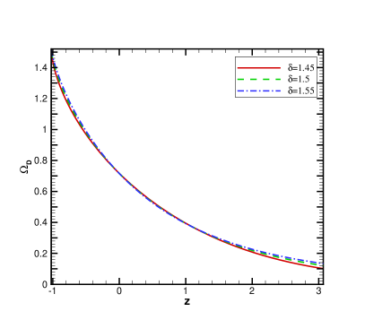
Figure 1: $\Omega_{D}$ versus $z$ for $\Omega_{D0}=0\cdot 73$, $u_{0}=0\cdot 3$, and some values of $\delta$.

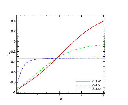
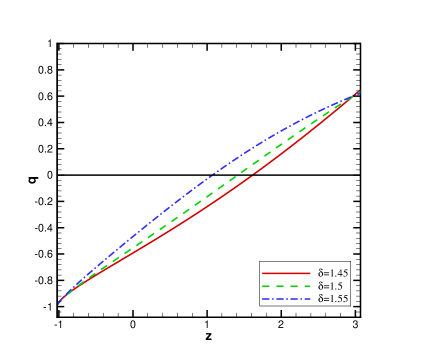
Figure 2: $\omega_{D}$ and $q$ versus $z$ for $\Omega_{D0}=0\cdot 73$ and some values of $\delta$ and $u_{0}=0\cdot 3$.

In Figs. 1 and 2, the behavior of the dimensionless density, EoS and deceleration parameters have been plotted against redshift $z$ by considering $\Omega_{D0}=0\cdot 73$ and $u_{0}=0\cdot 3$ for the current universe. As it is apparent from Fig. 2 and also confirmed by Eq. (11), we have $w_{D}\approx-1$ for DE dominant regime (or equally $u\approx 0$) which means that THDE in a cyclic universe simulates the cosmological constant model of DE at the late time. The results of employing original holographic dark energy model HDE5 in cyclic cosmology are also recovered at the $\delta=1$ limit Cyclic2 . In summary, the phantom line is not crossed in this model ($w_{D}\geq-1$), and the transition redshift $z_{t}$ from a deceleration phase to an accelerated universe lies within the interval $0\cdot 35<z_{t}<1$.

III THDE in DGP braneworld

For a flat FRW brane embedded in a Minkowski bulk, the Friedmann equation takes the form Deffayet ; Copeland

$$H^{2}=\Big{(}\sqrt{\frac{\rho}{3M_{\rm pl}^{2}}+\frac{1}{4r^{2}_{c}}}+\frac{\epsilon}{2r_{c}}\Big{)}^{2},$$ (13)

where $\rho$ includes the energy density of DM, $\rho_{m}$, and DE, $\rho_{D}$, on the brane, and $r_{c}=\frac{M_{\rm pl}^{2}}{2M_{5}^{3}}=\frac{G_{5}}{2G_{4}}$ denotes the crossover length scale between the small and large distances Deffayet . It is obvious that this equation is reduced to

$$H^{2}=\frac{\rho}{3M_{\rm pl}^{2}},$$ (14)

for $r_{c}\gg 1$, nothing but the standard Friedmann equation in flat FRW spacetime. Eq. (13) can also be written as

$$H^{2}-\frac{\epsilon}{r_{c}}H=\frac{\rho}{3M_{\rm pl}^{2}},$$ (15)

which reduces to

$$H^{2}=\frac{\rho^{2}}{36M_{5}^{6}},$$ (16)

for $\epsilon=-1$ and $r_{c}\ll H^{-1}$ RSII . This result clearly proves that this branch does not give the self-accelerating solution which compels us to consider a DE component on the brane to describe the current accelerated universe. Using Eq. (5) and $\Omega_{r_{c}}=\frac{1}{4H^{2}r_{c}^{2}}$, one can rewrite Eq. (15) as

$$\Omega_{m}+\Omega_{D}+2\epsilon\sqrt{\Omega_{r_{c}}}=1.$$ (17)

For a THDE (1) with the Hubble radius as IR cut off $(L=H^{-1})$, by using (5), we obtain

$$\Omega_{D}=\frac{BH^{2-2\delta}}{3M^{2}_{p}}.$$ (18)

Bearing in mind the time derivative of Eq. (1)

$$\dot{\rho}_{D}=2(2-\delta)\rho_{D}\frac{\dot{H}}{H},$$ (19)

and combining it with Eq. (18) and its time derivative, one finds

$$\Omega_{D}^{\prime}=2\Omega_{D}(1-\delta)\frac{\dot{H}}{H^{2}},$$ (20)

where prime denotes the derivative respect to $x=\ln a$, and we used $\dot{\Omega}_{D}=H\Omega_{D}^{\prime}$ to write the above relation. Now, combining the time derivative of Eq. (15) with Eqs. (4), (5) and (19), we get

$$\frac{\dot{H}}{H^{2}}=\frac{-3(1-\Omega_{D}-2\epsilon\sqrt{\Omega_{r_{c}}})}{2(\delta-2)\Omega_{D}-2\epsilon\sqrt{\Omega_{r_{c}}}+2},$$ (21)

which can be inserted into (20), to reach at

$$\Omega_{D}^{\prime}=\frac{3\Omega_{D}(1-\delta)(\Omega_{D}+2\epsilon\sqrt{\Omega_{r_{c}}}-1)}{(\delta-2)\Omega_{D}-\epsilon\sqrt{\Omega_{r_{c}}}+1}.$$ (22)

In the limiting case $r_{c}\gg 1$ (or equally $\Omega_{r_{c}}\rightarrow 0$), $\Omega_{D}$ of THDE in the Einstein theory Tavayef is restored, a desired result recovering the original HDE ($\Omega_{D}=const$) for $\delta=1$. The evolution of $\Omega_{D}$ as a function of redshift $z$ is plotted in Fig. (3) for different values of the parameter $\delta$, whenever $\epsilon=1$, $\Omega_{D}(z=0)\equiv\Omega_{D0}=0\cdot 73$ and $\Omega_{r_{c}}(z=0)=0\cdot 002$ Xu . Clearly, this figure indicates that we have $\Omega_{D}\rightarrow 0$ and $\Omega_{D}\rightarrow 1$, at the early Universe ($z\rightarrow\infty$) and the late time ($z\rightarrow-1$), respectively.

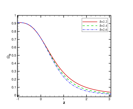
Figure 3: The evolution of $\Omega_{D}$ versus $z$ for $\Omega_{D0}=0\cdot 73$, $\Omega_{r_{c}0}=0\cdot 002$ Xu and some values of $\delta$.

Calculations of the EoS and deceleration parameters lead to

$$\omega_{D}=-1+\frac{(2-\delta)(1-\Omega_{D}-2\epsilon\sqrt{\Omega_{r_{c}}})}{(\delta-2)\Omega_{D}-\epsilon\sqrt{\Omega_{r_{c}}}+1},$$ (23)

and

$$q=-1+\frac{3(1-\Omega_{D}-2\epsilon\sqrt{\Omega_{r_{c}}})}{2(\delta-2)\Omega_{D}-2\epsilon\sqrt{\Omega_{r_{c}}}+2},$$ (24)

respectively, which are plotted in Fig. 4. One can easily see that for $r_{c}\gg 1$ $(\Omega_{r_{c}}\rightarrow 0)$, where the effects of extra dimension are negligible, the general relativity is recovered, and hence, Eqs. (23) and (24) decrease to their respective relations Tavayef . It is worth mentioning that, in the limiting case $\delta=1$, the relations of Ref. Ghaffari , as the desired result, are obtained. From Fig. 4, it is obvious that the model can cover the current accelerated universe even in the absence of a interaction between DM and DE. We also see that $\omega_{D}(z\rightarrow-1)\rightarrow-1$ which means that the model mimics the cosmological constant behavior at future. The transition redshift ($z_{t}$) from the acceleration phase to an accelerated phase lies within the $0\cdot 5<z_{t}<0\cdot 9$ range, which is completely consistent with the recent observations Daly ; Komatsu ; Salvatelli .

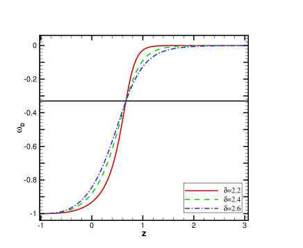
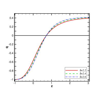
Figure 4: The evolution of the EoS parameter $\omega_{D}$ and deceletarion parameter $q$ versus redshift parameter $z$ for Tsallis HDE in DGP braneworld. We have taken $\epsilon=1$ and $\Omega_{r_{c}}=0\cdot 002$Xu as the initial conditions.

IV THDE in RS II braneworld

In RS II braneworld scenario, the modified Friedmann equation on the brane is written as

$$H^{2}+\frac{k}{a^{2}}=\frac{8\pi}{3M_{p}^{2}}\rho+\frac{8\pi}{3M_{p}^{2}}\rho_{\Lambda}$$ (25)

where $\rho$ denotes the total energy density of the pressureless source, $\rho_{m}$, and DE, $\rho_{\Lambda}$, on the brane, and $M_{p}^{2}=\frac{1}{8\pi G}$ is the reduced Planck mass. Following RS , the energy density of the four dimensional effective DE is given by

$$\rho_{\Lambda}\equiv\rho_{\Lambda 4}=\frac{M_{p}^{2}}{32\pi M_{5}^{3}}\rho_{\Lambda 5}+\frac{3M_{p}^{3}}{2\pi\Big{(}\frac{L_{5}}{8\pi}-2r_{c}\Big{)}^{2}},$$ (26)

where $\rho_{\Lambda 5}$ is the 5D bulk holographic dark energy, whichfor Tsallis HDE takes the following form

$$\rho_{\Lambda 5}=\frac{3c^{2}B}{4\pi}M_{5}^{3}L^{2\delta-4},$$ (27)

combined with Eq. (26) to get

$$\rho_{\Lambda}=\frac{3Bc^{2}M_{p}^{2}}{128\pi^{2}}L^{2\delta-4}+\frac{3M_{p}^{3}}{2\pi\Big{(}\frac{L_{5}}{8\pi}-2r_{c}\Big{)}^{2}},$$ (28)

for the effective $4$D THDE density. We can eliminate the second term in relation (28) for large values of $L$. Moreover, since $\rho_{\Lambda}\equiv\rho_{\Lambda 4}$ RS , we have

$$\rho_{\Lambda}=\frac{3Bc^{2}M_{p}^{2}}{128\pi^{2}}H^{4-2\delta}.$$ (29)

Using the definition (5), one can write Eq. (25) as follows

$$1+\Omega_{k}=\Omega_{m}+2\Omega_{\Lambda},$$ (30)

where

$$\Omega_{\Lambda}=\frac{Bc^{2}}{16\pi}H^{2-2\delta}.$$ (31)

Since the WMAP data indicates a flat FRW universe roos , we focus on the $k=0$ case from now on. In this manner, Eq. (30) indicates that whenever $\Omega_{m}$ is negligible, $\Omega_{\Lambda}$ gains its maximum value ($\frac{1}{2}$). Now, it is a matter of calculations to show that

$$\frac{\dot{H}}{H^{2}}=\frac{3(2\Omega_{\Lambda}-1)}{1+2\Omega_{\Lambda}(\delta-2)},$$ (32)

and

$$\Omega^{\prime}_{\Lambda}=\Omega_{\Lambda}(1-\delta)\frac{3(2\Omega_{\Lambda}-1)}{1+2\Omega_{\Lambda}(\delta-2)}.$$ (33)

The behavior of $\Omega_{D}$ against $z$ is plotted in Fig. 5, where the initial condition $\Omega_{D}(z=0)\equiv\Omega_{D0}=0\cdot 73$ has been considered. From this figure we clearly see that at the early universe ($z\rightarrow\infty$) we have $\Omega_{D}\rightarrow 0$, while at the late time ($z\rightarrow-1$), while DE will dominate and DM is ignorable, we have $\Omega_{D}\rightarrow 0\cdot 5$ in full agreement with Eq. (30).

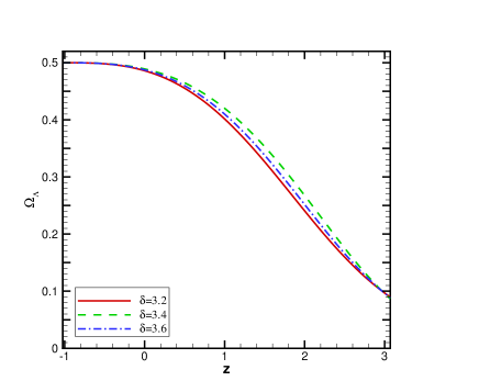
Figure 5: $\Omega_{D}$ for THDE in RS II braneworld. Here, we have taken $\Omega_{D0}=0\cdot 73$ as the initial condition.

For the EoS and deceleration parameters, one obtains

$$\omega_{\Lambda}=\frac{1-\delta}{1+2\Omega_{\Lambda}(\delta-2)},$$ (34)

and

$$q=-1-\frac{\dot{H}}{H^{2}}=-1+\frac{3(2\Omega_{\Lambda}-1)}{1+2\Omega_{\Lambda}(\delta-2)},$$ (35)

respectively. They are also depicted for different values of $\delta$ in Fig. 6. Our results indicate that the THDE model with the Hubble cutoff in the RSII braneworld can model the current accelerated universe, and admits the $0\cdot 5<z_{t}<0\cdot 9$ interval for the transition redshift, a result in full accordance with the recent observations Daly ; Komatsu ; Salvatelli .

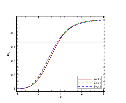
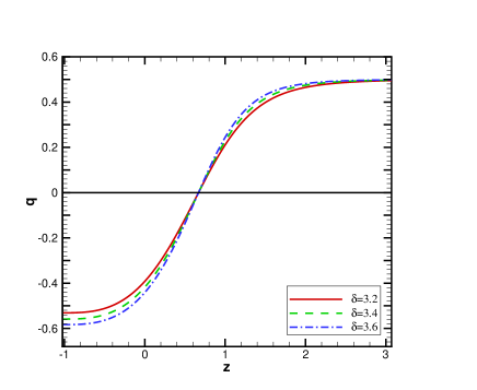
Figure 6: $\omega_{D}$ and $q$ versus $z$ for THDE in RS II brane for some values of $\delta$.

V Stability

In this section we would like to study the stability of models against small perturbations by using the squared of the sound speed ($v_{s}^{2}$). In fact, it can be found out by finding the sign of $v_{s}^{2}$. For $v_{s}^{2}>0$ the given perturbation propagates in the environment, and thus, the model is stable against perturbations. The squared sound speed $v_{s}^{2}$ is given by

$$v_{s}^{2}=\frac{dp}{d\rho_{D}}=\frac{\dot{p}}{\dot{\rho}_{D}},$$ (36)

where $P=P_{D}=\omega_{D}\rho_{D}$, and finally, we get

$$v_{s}^{2}=\omega_{D}+\frac{\dot{\omega}_{D}\rho_{D}}{\dot{\rho}_{D}}.$$ (37)

V.1 THDE in Cyclic univrse

By taking the time derivative of Eq. (11) and combining the result with Eqs. (9), (10) and (37), we can finally obtain the explicit expression of $v_{s}^{2}$ for THDE in cyclic universe. Since this expression is too long, we do not demonstrate it here, and we only plot it in Fig. 7 showing that, depending on the values of $\delta$, THDE in cyclic cosmology can not meet the stability requirement for all values of $\Omega_{D}$ (or equally $z$).

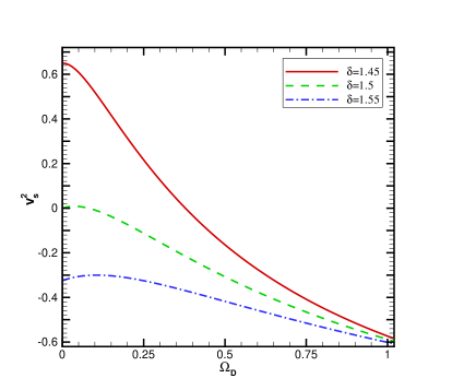
Figure 7: $v_{s}^{2}$ versus $\Omega_{D}$ for THDE in cyclic universe.

V.2 THDE in DGP braneworld

In this manner, calculations lead to

$$v_{s}^{2}=-1+\frac{(2-\delta)(1-\Omega_{D}-2\epsilon\sqrt{\Omega_{r_{c}}})}{(\delta-2)\Omega_{D}-\epsilon\sqrt{\Omega_{r_{c}}}+1}+$$ (38)

$$\frac{\Omega_{D}(\delta-1)\Big{(}(\delta-2)(1-2\epsilon\sqrt{\Omega_{r_{c}}})-\epsilon\sqrt{\Omega_{r_{c}}}+1\Big{)}}{((\delta-2)\Omega_{D}-\epsilon\sqrt{\Omega_{r_{c}}}+1)^{2}},$$

where behavior is shown in Fig 8 against $\Omega_{D}$. Clearly, we see that $v_{s}^{2}$ is ever negative indicating that THDE in DGP braneworld is always unstable against the perturbations for $2<\delta$. It is useful to note here that other values of $\delta$ cannot produce acceptable behavior for the system parameters including $\Omega_{D}$, $q$ and $\omega_{D}$.

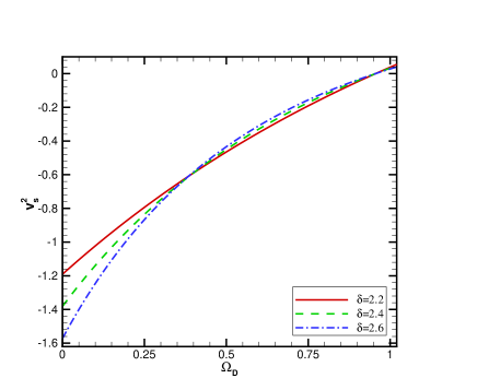
Figure 8: The evolution of $v_{s}^{2}$ versus $\Omega_{D}$ for THDE model in DGP braneworld, where $\epsilon=+1$ and $\Omega_{r_{c}0}=0\cdot 002$Xu .

V.3 THDE in RSII braneworld

Using Eqs. (37), (32), (33), and the time derivative of Eq. (34), one can find

$$v_{s}^{2}=\frac{(1-\delta)(1-2\Omega_{D})}{(1+2(2-\delta)\Omega_{D})^{2}},$$ (39)

where behavior is shown in Fig. 9. We conclude that THDE in RSII braneworld is stable for $\frac{1}{2}<\Omega_{D}<1$ while $\delta>1$. This result is in agreement with Eq. (39), and indeed, this Eq. (39) tells that the model is also stable for $0<\Omega_{D}<1/2$ whenever $0<\delta<1$.

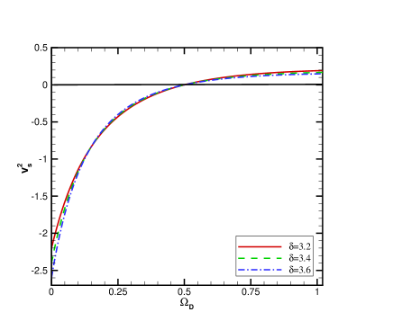
Figure 9: $v_{s}^{2}$ versus $\Omega_{D}$ for THDE in RS II braneworld.

VI CONCLUSION

We studied the cosmological consequences of THDE in the Cyclic, DGP and RS II models. In our study, we focused on a flat FRW brane filled with a pressureless dark matter and THDE, while there is no mutual interaction between them. Although all models may describe the current accelerated universe, none of them are always stable against small perturbations during the cosmic evolution, at least at the classical level. In fact, those values of $\delta$ leading the stable models can not produce acceptable behavior for $\omega_{D}$, $q$ and $\Omega_{D}$.