A Constraint-Reduced MPC Algorithm for Convex Quadratic Programming, with a Modified Active Set Identification Scheme

Abstract

A constraint-reduced Mehrotra–Predictor–Corrector algorithm for convex quadratic programming is proposed. (At each iteration, such algorithms use only a subset of the inequality constraints in constructing the search direction, resulting in CPU savings.) The proposed algorithm makes use of a regularization scheme to cater to cases where the reduced constraint matrix is rank deficient. Global and local convergence properties are established under arbitrary working-set selection rules subject to satisfaction of a general condition. A modified active-set identification scheme that fulfills this condition is introduced. Numerical tests show great promise for the proposed algorithm, in particular for its active-set identification scheme. While the focus of the present paper is on dense systems, application of the main ideas to large sparse systems is briefly discussed.

1 Introduction

Consider a strictly feasible convex quadratic program (CQP) in standard inequality form,

$$\operatorname*{minimize}_{\mathbf{x}\in\mathbb{R}^{n}}\>f(\mathbf{x}):=\frac{1}{2}\mathbf{x}^{T}H\mathbf{x}+\mathbf{c}^{T}\mathbf{x}\quad\mbox{subject to}\>A\mathbf{x}\geq\mathbf{b}\>,$$ (P)

where $\mathbf{x}\in\mathbb{R}^{n}$ is the vector of optimization variables, $f\colon\mathbb{R}^{n}\to\mathbb{R}$ is the objective function with $\mathbf{c}\in\mathbb{R}^{n}$ and $H\in\mathbb{R}^{n\times n}$ a symmetric positive semi-definite matrix, $A\in\mathbb{R}^{m\times n}$ and $\mathbf{b}\in\mathbb{R}^{m}$, with $m>0$, define the $m$ linear inequality constraints, and (here and elsewhere) all inequalities ($\geq$ or $\leq$) are meant component-wise. $H$, $A$, and $\mathbf{c}$ are not all zero. The dual problem associated to (P) is

$$\operatorname*{maximize}_{\mathbf{x}\in\mathbb{R}^{n},\,\boldsymbol{\lambda}\in\mathbb{R}^{m}}\>-\frac{1}{2}\mathbf{x}^{T}H\mathbf{x}+\mathbf{b}^{T}\boldsymbol{\lambda}\quad\mbox{subject to}\>H\mathbf{x}+\mathbf{c}-A^{T}\boldsymbol{\lambda}=\mathbf{0},\quad\boldsymbol{\lambda}\geq\mathbf{0}\>,$$ (D)

where $\boldsymbol{\lambda}\in\mathbb{R}^{m}$ is the vector of multipliers. Since the objective function $f$ is convex and the constraints are linear, solving (P)–(D) is equivalent to solving the Karush-Kuhn-Tucker (KKT) system

$$H\mathbf{x}-A^{T}\boldsymbol{\lambda}+\mathbf{c}=\mathbf{0},\quad A\mathbf{x}-\mathbf{b}-\mathbf{s}=\mathbf{0},\quad S\boldsymbol{\lambda}=\mathbf{0},\quad\mathbf{s},\boldsymbol{\lambda}\geq\mathbf{0}\>,$$ (1)

where $\mathbf{s}\in\mathbb{R}^{n}$ is a vector of slack variables associated to the inequality constraints in (P), and $S=\operatorname{diag}(\mathbf{s})$.

Primal–dual interior–point methods (PDIPM) solve (P)–(D) by iteratively applying a Newton-like iteration to the three equations in (1). Especially popular for its numerical behavior is S. Mehrotra’s predictor–corrector (MPC) variant, which was introduced in Mehrotra-1992 for the case of linear optimization (i.e., $H=\mathbf{0}$) with straightforward extension to CQP (e.g., (Nocedal-Wright-2006, , Section 16.6)). (Extension to linear complementarity problems was studied in Zhang1995 .)

A number of authors have paid special attention to “imbalanced” problems, in which the number of active constraints at the solution is small compared to the total number of constraints (in particular, cases in which $m\gg n$). In solving such problems, while most constraints are in a sense redundant, traditional IPMs devote much effort per iteration to solving large systems of linear equations that involve all $m$ constraints. In the 1990s, work toward reducing the computational burden by using only a small portion (“working set”) of the constraints in the search direction computation focused mainly on linear optimization Ye1990 ; DantzigYe91 ; Tone1993 ; DenHer:94 . This was also the case for TAW-06 , which may have been the first to consider such “constraint-reduction” schemes in the context of PDIPMs (vs. purely dual interior–point methods), and for its extensions HT12 ; WNTO-2012 ; WTA-2014 . Exceptions include the works of Jung et al. JOT-08 ; JOT-12 and of Park et al. Park-OLeary-2015 ; Park2016 ; in the former, an extension to CQP was considered, with an affine-scaling variant used as the “base” algorithm; in the latter, a constraint-reduced PDIPM for semi-definite optimization (which includes CQP as a special case) was proposed, for which polynomial complexity was proved. Another exception is the “QP-free” algorithm for inequality-constrained (smooth) nonlinear programming of Chen et al. CWH06 . There, a constraint-reduction approach is used where working sets are selected by means of the Facchinei–Fischer–Kanzow active set identification technique FFK98 .

In the linear-optimization case, the size of the working set is usually kept above (or no lower than) the number $n$ of variables in (P). It is indeed known that, in that case, if the set of solutions to (P) is nonempty and bounded, then a solution exists at which at least $n$ constraints are active. Further if fewer than $n$ constraints are included in the linear system that defines the search direction, then the default (Newton-KKT) system matrix is structurally singular.

When $H\not=\mathbf{0}$ though, the number of active constraints at solutions may be much less than $n$ and, at strictly feasible iterates, the Newton-KKT matrix is non-singular whenever the subspace spanned by the columns of $H$ and the working-set columns of $A^{T}$ has (full) dimension $n$. (In particular, of course, if $H$ is non-singular (i.e., is positive definite) the Newton-KKT matrix is non-singular even when the working set is empty—in which case the unconstrained Newton direction is obtained.) Hence, when solving a CQP, forcing the working set to have size at least $n$ is usually wasteful.

The present paper proposes a constraint-reduced MPC algorithm for CQP. The work borrows from JOT-12 (affine-scaling, convex quadratic programming) and is significantly inspired from WNTO-2012 (MPC, linear optimization), but improves on both in a number of ways—even for the case of linear optimization (i.e., when $H=\mathbf{0}$). Specifically,

• in contrast with JOT-12 ; WNTO-2012 (and CWH06 ), it does not involve a (CPU-expensive) rank estimation combined with an increase of the size of the working set when a rank condition fails; rather, it makes use of a regularization scheme adapted from WTA-2014 ;

• a general condition (Condition CSR) to be satisfied by the constraint-selection rule is proposed which, when satisfied, guarantees global and local quadratic convergence of the overall algorithm (under appropriate assumptions);

• a specific constraint-selection rule is introduced which, like in CWH06 (but unlike in JOT-12 ), does not impose any a priori lower bound on the size of the working set; this rule involves a modified active set identification scheme that builds on results from FFK98 ; numerical comparison shows that the new rule outperforms previously used rules.

Other improvements over JOT-12 ; WNTO-2012 include (i) a modified stopping criterion and a proof of termination of the algorithm (in JOT-12 ; WNTO-2012 , termination is only guaranteed under uniqueness of primal-dual solution and strict complementarity), (ii) a potentially larger value of the “mixing parameter” in the definition of the primal search direction (see footnote 2(iii)), and (iii) an improved update formula (compared to that used in WTA-2014 ) for the regularization parameter, which fosters a smooth evolution of the regularized Hessian $W$ from an initial (matrix) value $H+R$, where $R$ is specified by the user, at a rate no faster than that required for local q-quadratic convergence.

In Section 2 below, we introduce the proposed algorithm (Algorithm 2.2) and a general condition (Condition CSR) to be satisfied by the constraint-selection rule, and we state global and local quadratic convergence results for Algorithm 2.2, subject to Condition CSR. We conclude the section by proposing a specific rule (Rule R), and proving that it satisfies Condition CSR. Numerical results are reported in Section 3. While the focus of the present paper is on dense systems, application of the main ideas to large sparse systems is briefly discussed in the Conclusion (Section 4), which also includes other concluding remarks. Convergence proofs are given in two appendices.

The following notation is used throughout the paper. To the number $m$ of inequality constraints, we associate the index set $\mathbf{m}:=\{1,2,\ldots,m\}$. The primal feasible and primal strictly feasible sets are

$$\mathcal{F}_{P}:=\{\mathbf{x}\in\mathbb{R}^{n}:A\mathbf{x}\geq\mathbf{b}\}\quad\mbox{and}\quad\mathcal{F}_{P}^{o}:=\{\mathbf{x}\in\mathbb{R}^{n}:A\mathbf{x}>\mathbf{b}\},$$

and the primal and primal-dual solution sets are

$$\mathcal{F}_{P}^{*}:=\{\mathbf{x}\in\mathcal{F}_{P}:f(\mathbf{x})\leq f(\tilde{\mathbf{x}}),\,\forall\tilde{\mathbf{x}}\in\mathcal{F}_{P}\}\quad\mbox{and}\quad\mathcal{F}^{*}:=\{(\mathbf{x},\boldsymbol{\lambda}):\eqref{eq:KKT}{\rm~{}holds}\}\>.$$

Of course, $\mathbf{x}^{*}\in\mathcal{F}_{P}^{*}$ if and only if, for some $\boldsymbol{\lambda}^{*}\in\mathbb{R}^{m}$, $(\mathbf{x}^{*},\boldsymbol{\lambda}^{*})\in\mathcal{F}^{*}$ Also, we term stationary a point $\hat{\mathbf{x}}\in\mathcal{F}_{P}$ for which there exists $\hat{\boldsymbol{\lambda}}\in\mathbb{R}^{m}$ such that $(\hat{\mathbf{x}},\hat{\boldsymbol{\lambda}})$ satisfies (1) except possibly for non-negativity of the components of $\hat{\boldsymbol{\lambda}}$. Next, for $\mathbf{x}\in\mathcal{F}_{P}$, the (primal) active-constraint set at $\mathbf{x}$ is

$$\mathcal{A}(\mathbf{x}):=\{i\in\mathbf{m}:\mathbf{a}_{i}^{T}\mathbf{x}=b_{i}\}\>,$$

where $\mathbf{a}_{i}$ is the transpose of the $i$-th row of $A$. Given a subset $Q\subseteq\mathbf{m}$, $Q^{\textup{c}}$ indicates its complement in $\mathbf{m}$ and $|Q|$ its cardinality; for a vector $\mathbf{v}\in\mathbb{R}^{m}$, $\mathbf{v}_{Q}$ is a sub-vector consisting of those entries with index in $Q$, and for an $m\times n$ matrix $L$, $L_{Q}$ is a $|Q|\times n$ sub-matrix of $L$ consisting of those rows with index in $Q$. An exception to this rule, which should not create any confusion, is that for an $m\times m$ diagonal matrix $V=\operatorname{diag}(\mathbf{v})$, $V_{Q}$ is $\operatorname{diag}(\mathbf{v}_{Q})$, a $|Q|\times|Q|$ diagonal sub-matrix of $V$. For symmetric matrices $W$ and $H$, $W\succeq H$ (resp. $W\succ H$) means that $W-H$ is positive semi-definite (resp. positive definite). Finally, given a vector $\mathbf{v}$, $[\mathbf{v}]_{+}$ and $[\mathbf{v}]_{-}$ denote the positive and negative parts of $\mathbf{v}$, i.e., vectors with components respectively given by $\max\{v_{i},0\}$ and $\min\{v_{i},0\}$, $\mathbf{1}$ is a vector of all ones, and given a Euclidean space $\mathbb{R}^{p}$, the ball centered at $\mathbf{v}^{*}\in\mathbb{R}^{p}$ with radius $\rho>0$ is denoted by $B(\mathbf{v}^{*},\rho):=\{\mathbf{v}\in\mathbb{R}^{p}:\|\mathbf{v}-\mathbf{v}^{*}\|\leq\rho\}$.

2 A Regularized, Constraint-Reduced MPC Iteration

2.1 A Modified MPC Algorithm

In WNTO-2012 , a constraint-reduced MPC algorithm was proposed for linear optimization problems, as a constraint-reduced extension of a globally and locally superlinearly convergent variant of Mehrotra’s original algorithm Mehrotra-1992 ; Wright-1997 . Transposed to the CQP context, that variant proceeds as follows.

In a first step (following the basic MPC paradigm), given ($\mathbf{x}$, $\boldsymbol{\lambda}$, $\mathbf{s}$) with $\boldsymbol{\lambda}>\mathbf{0}$, $\mathbf{s}>\mathbf{0}$, it computes the primal–dual affine-scaling direction $(\Delta\mathbf{x}^{\textup{a}},\,\Delta\boldsymbol{\lambda}^{\textup{a}},\,\Delta\mathbf{s}^{\textup{a}})$ at $(\mathbf{x},\boldsymbol{\lambda},\mathbf{s})$, viz., the Newton direction for the solution of the equations portion of (1). Thus, it solves

$$J(H,A,\mathbf{s},\boldsymbol{\lambda})\left[\begin{array}[]{c}\Delta\mathbf{x}^{\textup{a}}\\ \Delta\boldsymbol{\lambda}^{\textup{a}}\\ \Delta\mathbf{s}^{\textup{a}}\end{array}\right]=\left[\begin{array}[]{c}-\nabla f(\mathbf{x})+A^{T}\boldsymbol{\lambda}\\ \mathbf{0}\\ -S\boldsymbol{\lambda}\end{array}\right]\>,$$ (2)

where, given a symmetric matrix $W\succeq\mathbf{0}$, we define

$$J(W,A,\mathbf{s},\boldsymbol{\lambda}):=\left[\begin{array}[]{ccc}W&-A^{T}&\mathbf{0}\\ A&\mathbf{0}&-I\\ \mathbf{0}&S&\Lambda\end{array}\right],$$

with $\Lambda=\operatorname{diag}(\boldsymbol{\lambda})$. Conditions for unique solvability of system (2) are given in the following standard result (invoked in its full form later in this paper); see, e.g., (JungThesis, , Lemma B.1).

Lemma 1

Suppose $s_{i},\lambda_{i}\geq 0$ for all $i$ and $W\succeq\mathbf{0}$. Then $J(W,A,\mathbf{s},\boldsymbol{\lambda})$ is invertible if and only if the following three conditions hold:

1. $s_{i}+\lambda_{i}>0$ for all $i$;

2. $A_{\{i:s_{i}=0\}}$ has full row rank; and

3. $\left[W\,\,\left(A_{\{i:\lambda_{i}\neq 0\}}\right)^{T}\right]$ has full row rank.

In particular, with $\boldsymbol{\lambda}>\mathbf{0}$ and $\mathbf{s}>\mathbf{0}$, $J(H,A,\mathbf{s},\boldsymbol{\lambda})$ is invertible if and only if $[H\,\,A^{T}]$ has full row rank. By means of two steps of block Gaussian elimination, system (2) reduces to the normal system

$$M\Delta\mathbf{x}^{\textup{a}} =-\nabla f(\mathbf{x}),$$ (3)

$$\Delta\mathbf{s}^{\textup{a}} =A\Delta\mathbf{x}^{\textup{a}},$$

$$\Delta\boldsymbol{\lambda}^{\textup{a}} =-\boldsymbol{\lambda}-S^{-1}\Lambda\Delta\mathbf{s}^{\textup{a}}\>,$$

where $M$ is given by

$$M:=H+A^{T}S^{-1}\Lambda A=H+\sum_{i=1}^{m}\frac{\lambda_{i}}{s_{i}}\mathbf{a}_{i}\mathbf{a}_{i}^{T}\>.$$ (4)

Given positive definite $S$ and $\Lambda$, $M$ is invertible whenever $J(H,A,\mathbf{s},\boldsymbol{\lambda})$ is.

In a second step, MPC algorithms construct a centering/corrector direction, which in the CQP case (e.g., (Nocedal-Wright-2006, , Section 16.6)) is the solution $(\Delta\mathbf{x}^{\textup{c}},\,\Delta\boldsymbol{\lambda}^{\textup{c}},\,\Delta\mathbf{s}^{\textup{c}})$ to (same coefficient matrix as in (2))

$$J(H,A,\mathbf{s},\boldsymbol{\lambda})\left[\begin{array}[]{c}\Delta\mathbf{x}^{\textup{c}}\\ \Delta\boldsymbol{\lambda}^{\textup{c}}\\ \Delta\mathbf{s}^{\textup{c}}\end{array}\right]=\left[\begin{array}[]{c}\mathbf{0}\\ \mathbf{0}\\ \sigma\mu\mathbf{1}-\Delta S^{\textup{a}}\Delta\boldsymbol{\lambda}^{\textup{a}}\end{array}\right]\>,$$ (5)

where $\mu:=\mathbf{s}^{T}\boldsymbol{\lambda}/m$ is the “duality measure” and $\sigma:=(1-\alpha^{\textup{a}})^{3}$ is the centering parameter, with

$$\alpha^{\textup{a}}:=\text{argmax}\{\alpha\in[0,\,1]\,|\,\mathbf{s}+\alpha\Delta\mathbf{s}^{\textup{a}}\geq\mathbf{0},\,\,\boldsymbol{\lambda}+\alpha\Delta\boldsymbol{\lambda}^{\textup{a}}\geq\mathbf{0}\}\>.$$

While most MPC algorithms use as search direction the sum of the affine-scaling and centering/corrector directions, to force global convergence, we borrow from WNTO-2012 and define

$$(\Delta\mathbf{x},\,\Delta\boldsymbol{\lambda},\,\Delta\mathbf{s})=(\Delta\mathbf{x}^{\textup{a}},\,\Delta\boldsymbol{\lambda}^{\textup{a}},\,\Delta\mathbf{s}^{\textup{a}})+\gamma(\Delta\mathbf{x}^{\textup{c}},\,\Delta\boldsymbol{\lambda}^{\textup{c}},\,\Delta\mathbf{s}^{\textup{c}}),$$ (6)

where the “mixing” parameter $\gamma\in[0,\,1]$ is one when $\Delta\mathbf{x}^{\textup{c}}=\mathbf{0}$ and otherwise

$$\gamma:=\min\left\{\gamma_{1},\,\tau\frac{\|\Delta\mathbf{x}^{\textup{a}}\|}{\|\Delta\mathbf{x}^{\textup{c}}\|},\,\tau\frac{\|\Delta\mathbf{x}^{\textup{a}}\|}{\sigma\mu}\right\},$$ (7)

where $\tau\in[0,1)$ and

$$\gamma_{1}:=\text{argmax}\left\{\tilde{\gamma}\in[0,\,1]~{}|~{}f(\mathbf{x})-f(\mathbf{x}+\Delta\mathbf{x}^{\textup{a}}+\tilde{\gamma}\Delta\mathbf{x}^{\textup{c}})\geq\omega(f(\mathbf{x})-f(\mathbf{x}+\Delta\mathbf{x}^{\textup{a}}))\right\},$$ (8)

with $\omega\in(0,\,1)$. The first term in (7) guarantees that the search direction is a direction of significant descent for the objective function (which in our context is central to forcing global convergence) while the other two terms ensures that the magnitude of the centering/corrector direction is not too large compared to the magnitude of the affine-scaling direction.

As for the line search, we again borrow from WNTO-2012 , where specific safeguards are imposed to guarantee global and local q-quadratic convergence. We set

$$\bar{\alpha}_{\textup{p}} :=\text{argmax}\{\alpha:\mathbf{s}+\alpha\Delta\mathbf{s}\geq\mathbf{0}\},\quad \alpha_{\textup{p}}:=\min\{1,\,\max\{\varkappa\bar{\alpha}_{\textup{p}},\,\bar{\alpha}_{\textup{p}}-\|\Delta\mathbf{x}\|\}\},$$

$$\bar{\alpha}_{\textup{d}} :=\text{argmax}\{\alpha:\boldsymbol{\lambda}+\alpha\Delta\boldsymbol{\lambda}\geq\mathbf{0}\},\quad \alpha_{\textup{d}}:=\min\{1,\,\max\{\varkappa\bar{\alpha}_{\textup{d}},\,\bar{\alpha}_{\textup{d}}-\|\Delta\mathbf{x}\|\}\}\>,$$

with $\varkappa\in(0,1)$, then

$$(\mathbf{x}^{+},\mathbf{s}^{+}):=(\mathbf{x},\mathbf{s})+\alpha_{\textup{p}}(\Delta\mathbf{x},\Delta\mathbf{s})\>.$$

and finally

$$\lambda^{+}_{i}:=\min\{\lambda^{\text{max}},\,\max\{{\lambda}_{i}+\alpha_{\textup{d}}\Delta\lambda_{i},\,\min\{\underline{\lambda},\,\chi\}\}\},\,i=1,\ldots,m\>,$$ (9)

where $\lambda^{\text{max}}>0$ and $\underline{\lambda}\in(0,\lambda^{\text{max}})$ are algorithm parameters, and

$$\chi:=\|\Delta\mathbf{x}^{\textup{a}}\|^{\nu}+\|[{\boldsymbol{\lambda}}+\Delta\boldsymbol{\lambda}^{\textup{a}}]_{-}\|^{\nu}\>,$$

with $\nu\geq 2$.

We verified via numerical tests that for the problems considered in Section 3, the modified MPC algorithm outlined in this section is at least as efficient as the MPC algorithm for CQPs given in (Nocedal-Wright-2006, , Algorithm 16.4).

2.2 A Regularized Constraint-Reduced MPC Algorithm

In the modified MPC algorithm described in Section 2.1, the main computational cost is incurred in forming the normal matrix $M$ (see (4)), which requires approximately $mn^{2}/2$ multiplications (at each iteration) if $A$ is dense, regardless of how many of the $m$ inequality constraints in (P) are active at the solution. This may be wasteful when few of these constraints are active at the solution, in particular (generically) when $m\gg n$ (imbalanced problems). The constraint-reduction mechanism introduced in TAW-06 and used in JOT-12 in the context of an affine-scaling algorithm for the solution of CQPs modifies $M$ by limiting the sum in (4) to a wisely selected small subset of terms, indexed by an index set $Q\subseteq\mathbf{m}$ referred to as the working set.

Given a working set $Q$, the constraint-reduction technique produces an approximate affine-scaling direction by solving a “reduced” version of the Newton system (2), viz.

$$J(H,A_{Q},\mathbf{s}_{Q},\boldsymbol{\lambda}_{Q})\left[\begin{array}[]{c}\Delta\mathbf{x}^{\textup{a}}\\ \Delta\boldsymbol{\lambda}_{Q}^{\textup{a}}\\ \Delta\mathbf{s}_{Q}^{\textup{a}}\end{array}\right]=\left[\begin{array}[]{c}-\nabla f(\mathbf{x})+(A_{Q})^{T}\boldsymbol{\lambda}_{Q}\\ \mathbf{0}\\ -S_{Q}\boldsymbol{\lambda}_{Q}\end{array}\right]\>.$$ (10)

Just like the full system, when $\mathbf{s}_{Q}>\mathbf{0}$, the reduced system (10) is equivalent to the reduced normal system

$$\tilde{M}_{(Q)}\Delta\mathbf{x}^{\textup{a}} =-\nabla f(\mathbf{x})\>,$$ (11)

$$\Delta\mathbf{s}_{Q}^{\textup{a}} =A_{Q}\Delta\mathbf{x}^{\textup{a}}\>,$$

$$\Delta\boldsymbol{\lambda}^{\textup{a}}_{Q} =-\boldsymbol{\lambda}_{Q}-S_{Q}^{-1}\Lambda_{Q}\Delta\mathbf{s}_{Q}^{\textup{a}}\>,$$

where the “reduced” $\tilde{M}_{(Q)}$ (still of size $n\times n$) is given by

$$\tilde{M}_{(Q)}:=H+(A_{Q})^{T}S_{Q}^{-1}\Lambda_{Q}A_{Q}=H+\sum_{i\in Q}\frac{\lambda_{i}}{s_{i}}\mathbf{a}_{i}\mathbf{a}_{i}^{T}\>.$$

When $A$ is dense, the cost of forming $\tilde{M}_{(Q)}$ is approximately $qn^{2}/2$, where $q:=|Q|$, leading to significant savings when $q\ll m$.

One difficulty that may arise, when substituting $A_{Q}$ for $A$ in the Newton-KKT matrix, is that the resulting linear system might no longer be uniquely solvable. Indeed, even when $[H\,\,A^{T}]$ has full row rank, $[H\,\,(A_{Q})^{T}]$ may be rank-deficient, so the third condition in Lemma 1 would not hold. A possible remedy is to regularize the linear system. In the context of linear optimization, such regularization was implemented in Gill-1994 and explored in Saunders-Tomlin-1996 by effectively adding a fixed scalar multiple of identity matrix into the normal matrix to improve numerical stability of the Cholesky factorization. A more general regularization was proposed in Altman-Gondzio-1999 where diagonal matrices that are adjusted dynamically based on the pivot values in the Cholesky factorization were used for regularization. On the other hand, quadratic regularization was applied to obtain better preconditioners in Castro-Cuesta-2011 , where a hybrid scheme of the Cholesky factorization and a preconditioned conjugate gradient method is used to solve linear systems arising in primal block-angular problems. In Castro-Cuesta-2011 , the regularization dies out when optimality is approached.

Applying regularization to address rank-deficiency of the normal matrix due to constraint reduction was first considered in WTA-2014 , in the context of linear optimization. There a similar regularization as in Gill-1994 ; Saunders-Tomlin-1996 is applied, while the scheme lets the regularization die out as a solution to the optimization problem is approached, to preserve fast local convergence. Adapting such approach to the present context, we replace $J(H,A_{Q},\mathbf{s}_{Q},\boldsymbol{\lambda}_{Q})$ by $J(W,A_{Q},\mathbf{s}_{Q},\boldsymbol{\lambda}_{Q})$ and $\tilde{M}_{(Q)}$ by

$$M_{(Q)}:=W+(A_{Q})^{T}S_{Q}^{-1}\Lambda_{Q}A_{Q}\>,$$ (12)

with $W:=H+\varrho R$, where $\varrho\in(0,1]$ is a regularization parameter that is updated at each iteration and $R\succeq\mathbf{0}$ a constant symmetric matrix such that $H+R\succ\mathbf{0}$. Thus the inequality $W\succeq H$ is enforced, ensuring $f(\mathbf{x}+\Delta\mathbf{x}^{\textup{a}})<f(\mathbf{x})$ (see Proposition 2 below), which in our context is critical for global convergence. In the proposed algorithm, the modified coefficient matrix is used in the computation of both a modified affine-scaling direction and a modified centering/corrector direction, which thus solves

$$J(W,A_{Q},\mathbf{s}_{Q},\boldsymbol{\lambda}_{Q})\left[\begin{array}[]{c}\Delta\mathbf{x}^{\textup{c}}\\ \Delta\boldsymbol{\lambda}_{Q}^{\textup{c}}\\ \Delta\mathbf{s}_{Q}^{\textup{c}}\end{array}\right]=\left[\begin{array}[]{c}\mathbf{0}\\ \mathbf{0}\\ \sigma\mu_{(Q)}\mathbf{1}-\Delta S_{Q}^{\textup{a}}\Delta\boldsymbol{\lambda}_{Q}^{\textup{a}}\end{array}\right]\>.$$ (13)

In the bottom block of the right-hand side of (13) (compared to (5)) we have substituted $\Delta S_{Q}^{\textup{a}}$ and $\Delta\boldsymbol{\lambda}_{Q}^{\textup{a}}$ for $\Delta S^{\textup{a}}$ and $\Delta\boldsymbol{\lambda}^{\textup{a}}$, and replaced $\mu$ with

$$\mu_{(Q)}:=\begin{cases}\mathbf{s}_{Q}^{T}\boldsymbol{\lambda}_{Q}/q\>,&\text{if }q\neq 0\\ 0\>,&\text{otherwise}\end{cases}\>,$$ (14)

the duality measure for the “reduced” problem. The corresponding normal equation system is given by

$$M_{(Q)}\Delta\mathbf{x}^{\textup{c}} =(A_{Q})^{T}S_{Q}^{-1}(\sigma\mu_{(Q)}\mathbf{1}-\Delta S_{Q}^{\textup{a}}\Delta\boldsymbol{\lambda}_{Q}^{\textup{a}}),$$ (15)

$$\Delta\mathbf{s}_{Q}^{\textup{c}} =A_{Q}\Delta\mathbf{x}^{\textup{c}},$$

$$\Delta\boldsymbol{\lambda}_{Q}^{\textup{c}} =S_{Q}^{-1}(-\Lambda_{Q}\Delta\mathbf{s}_{Q}^{\textup{c}}+\sigma\mu_{(Q)}\mathbf{1}-\Delta S_{Q}^{\textup{a}}\Delta\boldsymbol{\lambda}_{Q}^{\textup{a}})\>.$$

A partial search direction for the constraint-reduced MPC algorithm at $(\mathbf{x},\,\boldsymbol{\lambda},\,\mathbf{s})$ is then given by (see (6))

$$(\Delta\mathbf{x},\,\Delta\boldsymbol{\lambda}_{Q},\,\Delta\mathbf{s}_{Q})=(\Delta\mathbf{x}^{\textup{a}},\,\Delta\boldsymbol{\lambda}^{\textup{a}}_{Q},\,\Delta\mathbf{s}^{\textup{a}}_{Q})+\gamma(\Delta\mathbf{x}^{\textup{c}},\,\Delta\boldsymbol{\lambda}^{\textup{c}}_{Q},\,\Delta\mathbf{s}^{\textup{c}}_{Q}),$$ (16)

where $\gamma$ is given by (7)–(8), with $\mu_{(Q)}$ replacing $\mu$.

Algorithm 2.2, including a stopping criterion, a simple update rule for $\varrho$, and update rules (adapted from WNTO-2012 ) for the components $\lambda_{i}$ of the dual variable with $i\in Q^{\textup{c}}$, but with the constraint-selection rule (in Step 2) left unspecified, is formally stated below. Its core, Iteration 2.2, takes as input the current iterates $\mathbf{x}$, $\mathbf{s}>0$, $\boldsymbol{\lambda}>0$, $\tilde{\boldsymbol{\lambda}}$, and produces the next iterates $\mathbf{x}^{+}$, $\mathbf{s}^{+}>0$, $\boldsymbol{\lambda}^{+}>0$, $\tilde{\boldsymbol{\lambda}}^{+}$, used as input to the next iteration. Here $\tilde{\boldsymbol{\lambda}}$, with possibly $\tilde{\boldsymbol{\lambda}}\not\geq 0$, is asymptotically slightly closer to optimality than $\boldsymbol{\lambda}$, and is used in the stopping criterion. While dual feasibility of $(\mathbf{x},\boldsymbol{\lambda})$ is not enforced along the sequence of iterates, a primal strictly feasible starting point $\mathbf{x}\in\mathcal{F}_{P}^{o}$ is required, and primal feasibility of subsequent iterates is enforced, as it allows for monotone descent of $f$, which in the present context is key to global convergence. (An extension of Algorithm 2.2 that allows for infeasible starting points is discussed in Section 2.3 below.) Algorithm 2.2 makes use (in its stopping criterion and $\varrho$ update) of an “error” function $E\colon\mathbb{R}^{n}\times\mathbb{R}^{m}\to\mathbb{R}$ (also used in the constraint-selection Rule R in Section 2.6 below) given by

$$E(\mathbf{x},\boldsymbol{\lambda}):=\left\|(\|\mathbf{v}(\mathbf{x},\boldsymbol{\lambda})\|,\|\mathbf{w}(\mathbf{x},\boldsymbol{\lambda})\|)\right\|\>,$$ (17)

where

$$\mathbf{v}(\mathbf{x},\boldsymbol{\lambda}):=H\mathbf{x}+\mathbf{c}-A^{T}\boldsymbol{\lambda},\quad w_{i}(\mathbf{x},\boldsymbol{\lambda}):=\min\{|s_{i}|,|\lambda_{i}|\},~{}i=1,\ldots,m,$$ (18)

with $\mathbf{s}:=A\mathbf{x}-\mathbf{b}$, and where the norms are arbitrary. Here $E$ measures both dual feasibility (via $\mathbf{v}$) and complementary slackness (via $\mathbf{w}$). Note that, for $\mathbf{x}\in\mathcal{F}_{P}$ and $\boldsymbol{\lambda}\geq\mathbf{0}$, $E(\mathbf{x},\boldsymbol{\lambda})=0$ if and only if $(\mathbf{x},\boldsymbol{\lambda})$ solves (P)–(D).

 

Algorithm CR-MPC: A Constraint-Reduced variant of MPC Algorithm for CQP

1:Parameters: $\varepsilon\geq 0$, $\tau\in[0,1)$, $\omega\in(0,1)$, $\varkappa\in(0,1)$, $\nu\geq 2$, $\lambda^{\max}>0$, $\underline{\lambda}\in(0,\lambda^{\max})$, and $\bar{E}>0$. A symmetric $n\times n$ matrix $R\succeq\mathbf{0}$ such that $H+R\succ\mathbf{0}$.

2:Initialization: $\mathbf{x}\in\mathcal{F}_{P}^{o}$, $\boldsymbol{\lambda}>\mathbf{0}$, $\mathbf{s}:=A\mathbf{x}-\mathbf{b}>\mathbf{0}$, $\tilde{\boldsymbol{\lambda}}:=\boldsymbol{\lambda}$.

3:Iteration CR-MPC:

4:Step 1. Terminate if either (i) $\nabla f(\mathbf{x})=\mathbf{0}$, in which case $(\mathbf{x},\mathbf{0})$ is optimal for (P)–(D), or (ii)

$$\min\left\{E(\mathbf{x},\boldsymbol{\lambda}),E(\mathbf{x},[\tilde{\boldsymbol{\lambda}}]_{+})\right\}<\varepsilon,$$ (19)

in which case $(\mathbf{x},[\tilde{\boldsymbol{\lambda}}]_{+})$ is declared $\varepsilon$-optimal for (P)–(D) if $E(\mathbf{x},\boldsymbol{\lambda})\geq E(\mathbf{x},[\tilde{\boldsymbol{\lambda}}]_{+})$, and $(\mathbf{x},\boldsymbol{\lambda})$ is otherwise.

5:Step 2. Select a working set $Q$. Set $q:=|Q|$. Set $\varrho:=\min\{1,\frac{E(\mathbf{x},\boldsymbol{\lambda})}{\bar{E}}\}$. Set $W:=H+\varrho R$.

6:Step 3. Compute approximate normal matrix $M_{(Q)}:=W+\sum_{i\in Q}\frac{\lambda_{i}}{s_{i}}\mathbf{a}_{i}\mathbf{a}_{i}^{T}$.

7:Step 4. Solve

$$M_{(Q)}\Delta\mathbf{x}^{\textup{a}}=-\nabla f(\mathbf{x})\>,$$ (20)

and set

$$\Delta\mathbf{s}^{\textup{a}}:=A\Delta\mathbf{x}^{\textup{a}}\>,\quad\Delta\boldsymbol{\lambda}^{\textup{a}}_{Q}:=-\boldsymbol{\lambda}_{Q}-S_{Q}^{-1}\Lambda_{Q}\Delta\mathbf{s}_{Q}^{\textup{a}}\>.$$ (21)

8:Step 5. Compute the affine-scaling step

$$\alpha^{\textup{a}}:=\text{argmax}\{\alpha\in[0,\,1]\,|\,\mathbf{s}+\alpha\Delta\mathbf{s}^{\textup{a}}\geq\mathbf{0},\,\,\boldsymbol{\lambda}_{Q}+\alpha\Delta\boldsymbol{\lambda}^{\textup{a}}_{Q}\geq\mathbf{0}\}\>.$$ (22)

9:Step 6. Set $\mu_{(Q)}$ as in (14). Compute centering parameter $\sigma:=(1-\alpha^{\textup{a}})^{3}$.

10:Step 7. Solve (13) for the corrector direction $(\Delta\mathbf{x}^{\textup{c}},\,\Delta\boldsymbol{\lambda}_{Q}^{\textup{c}},\,\Delta\mathbf{s}_{Q}^{\textup{c}})$, and set $\Delta\mathbf{s}^{\textup{c}}:=A\Delta\mathbf{x}^{\textup{c}}$.

11:Step 8. If $q=0$, set $\gamma:=0$. Otherwise, compute $\gamma$ as in (7)–(8), with $\mu_{(Q)}$ replacing $\mu$. Compute the search direction

$$(\Delta\mathbf{x},\,\Delta\boldsymbol{\lambda}_{Q},\,\Delta\mathbf{s}):=(\Delta\mathbf{x}^{\textup{a}},\,\Delta\boldsymbol{\lambda}_{Q}^{\textup{a}},\,\Delta\mathbf{s}^{\textup{a}})+\gamma(\Delta\mathbf{x}^{\textup{c}},\,\Delta\boldsymbol{\lambda}_{Q}^{\textup{c}},\,\Delta\mathbf{s}^{\textup{c}})\>.$$ (23)

Set $\tilde{\lambda}^{+}_{i}=\lambda_{i}+\Delta\lambda_{i}$, $\forall i\in Q$, and $\tilde{\lambda}^{+}_{i}=0$, $\forall i\in Q^{\textup{c}}$.

12:Step 9. Compute the primal and dual steps $\alpha_{\textup{p}}$ and $\alpha_{\textup{d}}$ by

$$\bar{\alpha}_{\textup{p}} :=\text{argmax}\{\alpha:\mathbf{s}+\alpha\Delta\mathbf{s}\geq\mathbf{0}\},\quad \alpha_{\textup{p}}:=\min\{1,\,\max\{\varkappa\bar{\alpha}_{\textup{p}},\,\bar{\alpha}_{\textup{p}}-\|\Delta\mathbf{x}\|\}\},$$ (24)

$$\bar{\alpha}_{\textup{d}} :=\text{argmax}\{\alpha:\boldsymbol{\lambda}_{Q}+\alpha\Delta\boldsymbol{\lambda}_{Q}\geq\mathbf{0}\},\quad \alpha_{\textup{d}}:=\min\{1,\,\max\{\varkappa\bar{\alpha}_{\textup{d}},\,\bar{\alpha}_{\textup{d}}-\|\Delta\mathbf{x}\|\}\}\>.$$

13:Step 10. Updates:

$$(\mathbf{x}^{+},\mathbf{s}^{+}):=(\mathbf{x},\mathbf{s})+(\alpha_{\textup{p}}\Delta\mathbf{x},\alpha_{\textup{p}}\Delta\mathbf{s})\>.$$ (25)

Set $\chi:=\|\Delta\mathbf{x}^{\textup{a}}\|^{\nu}+\|[\boldsymbol{\lambda}_{Q}+\Delta\boldsymbol{\lambda}_{Q}^{\textup{a}}]_{-}\|^{\nu}$. Set

$$\lambda^{+}_{i}:=\max\{\min\{\lambda_{i}+\alpha_{\textup{d}}\Delta\lambda_{i},\,\lambda^{\text{max}}\},\,\min\{\chi,\,\underline{\lambda}\}\},\,\forall i\in Q\>.$$ (26)

Set $\mu_{(Q)}^{+}:={(\mathbf{s}_{Q}^{+})^{T}(\boldsymbol{\lambda}_{Q}^{+})}/{q}$ if $q\neq 0$, otherwise set $\mu_{(Q)}^{+}:=0$. Set

$$\lambda^{+}_{i}:=\max\{\min\{{\mu_{(Q)}^{+}}/{s_{i}^{+}},\,\lambda^{\text{max}}\},\,\min\{\chi,\,\underline{\lambda}\}\},\,\forall i\in Q^{\textup{c}}\>.$$ (27)

 

A few more comments are in order concerning Algorithm 2.2. First, the stopping criterion is a variation on that of JOT-12 ; WNTO-2012 , involving both $\boldsymbol{\lambda}$ and $[\tilde{\boldsymbol{\lambda}}]_{+}$ instead of only $\boldsymbol{\lambda}$; in fact the latter will fail when the parameter $\lambda^{\max}$ (see (26)–(27)) is not large enough and may fail when second order sufficient conditions are not satisfied, while we prove below (Theorem 2.1(iv)) that the new criterion is eventually satisfied indeed, in that the iterate $(\mathbf{x},\boldsymbol{\lambda})$ converges to a solution (even if it is not unique), be it on a mere subsequence. Second, our update formula for the regularization parameter $\varrho$ in Step 2 improves on that in WTA-2014 ($\varrho^{+}=\min\{\chi,\chi_{\max}\}$ in the notation of this paper, where $\chi_{\max}$ is a user-defined constant) as it fosters a “smooth” evolution of $W$ from the initial value of $H+R$, with $R$ specified by the user, at a rate no faster than that required for local q-quadratic convergence. And third, $R\succeq 0$ should be selected to compensate for possible ill-conditioning of $H$—so as to mitigate possible early ill-conditioning of $M_{(Q)}$. (Note that a nonzero $R$ may be beneficial even when $H$ is non-singular.)

It is readily established that, starting from a strictly feasible point, regardless of the choice made for $Q$ in Step 2, Algorithm 2.2 either stops at Step 1 after finitely many iterations, or generates infinite sequences $\{E_{k}\}_{k=0}^{\infty}$, $\{\mathbf{x}^{k}\}_{k=0}^{\infty}$, $\{\boldsymbol{\lambda}^{k}\}_{k=0}^{\infty}$, $\{\tilde{\boldsymbol{\lambda}}^{k}\}_{k=0}^{\infty}$, $\{\mathbf{s}^{k}\}_{k=0}^{\infty}$, $\{\chi_{k}\}_{k=0}^{\infty}$, $\{Q_{k}\}_{k=0}^{\infty}$, $\{\varrho_{k}\}_{k=0}^{\infty}$, and $\{W_{k}\}_{k=0}^{\infty}$, with $\mathbf{s}^{k}=A\mathbf{x}^{k}-\mathbf{b}>\mathbf{0}$ and $\boldsymbol{\lambda}^{k}>\mathbf{0}$ for all $k$. ($E_{0}$, $\chi_{0}$, $\varrho_{0}$, and $W_{0}$ correspond to the values of $E_{k}$, $\chi_{k}$, $\varrho_{k}$, and $W_{k}$ computed in the initial iteration, while the other initial values are provided in the “Initialization” step.) Indeed, if the algorithm does not terminate at Step 1, then $\nabla f(\mathbf{x})\not=\mathbf{0}$, i.e., $\Delta\mathbf{x}^{\textup{a}}\not=\mathbf{0}$ (from (20), since $M_{(Q)}$ is invertible); it follows that $\Delta\mathbf{x}\not=\mathbf{0}$ (if $\Delta\mathbf{x}^{\textup{c}}\not=\mathbf{0}$, since $\tau\in[0,1)$, (7) yields $\gamma<\|\Delta\mathbf{x}^{\textup{a}}\|/\|\Delta\mathbf{x}^{\textup{c}}\|$) and, since $\Delta\mathbf{x}^{\textup{a}}\not=\mathbf{0}$ implies $\chi>0$, (24), (23), (25), (26), and (27) imply that $\mathbf{s}^{+}=A\mathbf{x}^{+}-\mathbf{b}>\mathbf{0}$ and $\boldsymbol{\lambda}^{+}>\mathbf{0}$. From now on, we assume that infinite sequences are generated.

2.3 Extensions: Infeasible Starting Point, Equality Constraints

Because, in our constraint-reduction context, convergence is achieved by enforcing descent of the objective function at every iteration, infeasible starts cannot be accommodated as, e.g., in S. Mehrotra’s original paper Mehrotra-1992 . The penalty-function approach proposed and analyzed in (He-Thesis, , Chapter 3) in the context of constraint-reduced affine scaling for CQP (adapted from a scheme introduced in TWBUL-2003 for a nonlinear optimization context) fits right in however. (Also see HT12 for the linear optimization case.) Translated to the notation of the present paper, it substitutes for (P)–(D) the primal-dual pair

$$\operatorname*{minimize}_{\mathbf{x}\in\mathbb{R}^{n},\,\mathbf{z}\in\mathbb{R}^{m}}\>f(\mathbf{x})+\varphi\mathbf{1}^{T}\mathbf{z}\quad\mbox{s.t.~{}}\>A\mathbf{x}+\mathbf{z}\geq\mathbf{b}\>,\mathbf{z}\geq\mathbf{0}\>,$$ (P_φ)

$$\operatorname*{maximize}_{\mathbf{x}\in\mathbb{R}^{n},\,\boldsymbol{\lambda}\in\mathbb{R}^{m},\mathbf{u}\in\mathbb{R}^{m}}\>-\frac{1}{2}\mathbf{x}^{T}H\mathbf{x}+\mathbf{b}^{T}\boldsymbol{\lambda}\mbox{~{}s.t.~{}}\>H\mathbf{x}+\mathbf{c}-A^{T}\boldsymbol{\lambda}=\mathbf{0}\>,\boldsymbol{\lambda}+\mathbf{u}=\varphi\mathbf{1},(\boldsymbol{\lambda},\mathbf{u})\geq\mathbf{0},$$ (D_φ)

with $\varphi>0$ a scalar penalty parameter, for which primal-strictly-feasible points $(\mathbf{x},\mathbf{z})$ are readily available. Hence, given $\varphi$, this problem can be handled by Algorithm 2.2. Such $\ell_{1}$ penalty function is known to be exact, i.e., for some unknown, sufficiently large (but still moderate) value of $\varphi$, solutions $(\mathbf{x}^{*},\mathbf{z}^{*})$ to (P_φ) are such that $\mathbf{x}^{*}$ solves (P); further (He-Thesis ; HT12 ), $\mathbf{z}^{*}=\mathbf{0}$. In He-Thesis ; HT12 , an adaptive scheme is proposed for increasing $\varphi$ to such value. Applying this scheme on (P_φ)–(D_φ) allows Algorithm 2.2 to handle infeasible starting points for (P)–(D). We refer the reader to (He-Thesis, , Chapter 3) for details.

Linear equality constraints of course can be handled by first projecting the problem on the associated affine space, and then run Algorithm 2.2 on that affine space. A weakness of this approach though is that it does not adequately extend to the case of sparse problems (discussed in the Conclusion section (Section 4) of this paper), as projection may destroy sparsity. An alternative approach is, again, via augmentation: Given the constraints $C\mathbf{x}=\mathbf{d}$, with $\mathbf{d}\in\mathbb{R}^{p}$, solve the problem

$$\operatorname*{minimize}_{\mathbf{x}\in\mathbb{R}^{n},\,\mathbf{y}\in\mathbb{R}^{p}}\>f(\mathbf{x})+\varphi\mathbf{1}^{T}\mathbf{y}\quad\mbox{s.t.~{}}\>C\mathbf{x}+\mathbf{y}\geq\mathbf{d}\>,~{}C\mathbf{x}-\mathbf{y}\leq\mathbf{d}\>.$$ (28)

(Note that, taken together, the two constraints imply $\mathbf{y}\geq\mathbf{0}$.) Again, given $\varphi>0$ and using the same adaptive scheme from He-Thesis ; HT12 , this problem can be tackled by Algorithm 2.2.

2.4 A Class of Constraint-Selection Rules

Of course, the quality of the search directions is highly dependent on the choice of the working set $Q$. Several constraint-selection rules have been proposed for constraint-reduced algorithms on various classes of optimization problems, such as linear optimization WNTO-2012 ; WTA-2014 ; TAW-06 , convex quadratic optimization JOT-12 ; JOT-08 , semi-definite optimization Park-OLeary-2015 ; Park2016 , and nonlinear optimization CWH06 . In WNTO-2012 ; TAW-06 ; WTA-2014 , the cardinality $q$ of $Q$ is constant and decided at the outset. Because in the non-degenerate case the set of active constraints at the solution of (P) with $H=\mathbf{0}$ is at least equal to the number $n$ of primal variables, $q\geq n$ is usually enforced in that context. In JOT-12 , which like this paper deals with quadratic problems, $q$ was allowed to vary from iteration from iteration, but $q\geq n$ was still enforced throughout (owing to the fact that, in the regular case, there are no more than $n$ active constraints at the solution). Here we propose to again allow $q$ to vary, but in addition to not a priori impose a positive lower bound on $q$.

The convergence results stated in Section 2.5 below are valid with any constraint-selection rule that satisfies the following condition.

Condition CSR

Let $\{(\mathbf{x}^{k},\boldsymbol{\lambda}^{k})\}$ be the sequence constructed by Algorithm 2.2 with the constraint-selection rule under consideration, and let $Q_{k}$ be the working set generated by the constraint-selection rule at iteration $k$. Then the following holds: (i) if $\{(\mathbf{x}^{k},\boldsymbol{\lambda}^{k})\}$ is bounded away from $\mathcal{F}^{*}$, then, for all limit points $\mathbf{x}^{\prime}$ such that $\{\mathbf{x}^{k}\}\to\mathbf{x}^{\prime}$ on some infinite index set $K$, $\mathcal{A}(\mathbf{x}^{\prime})\subseteq Q_{k}$ for all large enough $k\in K$; and (ii) if (P)–(D) has a unique solution $(\mathbf{x}^{*},\boldsymbol{\lambda}^{*})$ and strict complementarity holds at $\mathbf{x}^{*}$, and if $\{\mathbf{x}^{k}\}\to\mathbf{x}^{*}$, then $\mathcal{A}(\mathbf{x}^{*})\subseteq Q_{k}$ for all $k$ large enough.

Condition CSR(i) aims at preventing convergence to non-optimal primal point, and hence (given a bounded sequence of iterates) forcing convergence to solution points. Condition CSR(ii) is important for fast local convergence to set in. A specific rule that satisfies Condition CSR, Rule R, used in our numerical experiments, is presented in Section 2.6 below.

2.5 Convergence Properties

The following standard assumptions are used in portions of the analysis.

Assumption 1

$\mathcal{F}_{P}^{o}$ is nonempty and $\mathcal{F}_{P}^{*}$ is nonempty and bounded  .

Assumption 2

At every stationary point $\mathbf{x}$, $A_{\mathcal{A}(\mathbf{x})}$ has full row rank.

Assumption 3

There exists a (unique) $\mathbf{x}^{*}$ where the second-order sufficient condition of optimality with strict complementarity holds, with (unique) $\boldsymbol{\lambda}^{*}$.

Assumption 3, mostly used in the local analysis, subsumes Assumption 9.

Theorem 2.1, proved in Appendix A, addresses global convergence.

Theorem 2.1

Suppose that the constraint-selection rule invoked in Step 2 of Algorithm 2.2 satisfies Condition CSR. First suppose that $\varepsilon=0$, that the iteration never stops, and that Assumptions 9 and 2 hold. Then (i) the infinite sequence $\{\mathbf{x}^{k}\}$ it constructs converges to the primal solution set $\mathcal{F}_{P}^{*}$; if in addition, Assumption 3 holds, then (ii) $\{(\mathbf{x}^{k},\tilde{\boldsymbol{\lambda}}^{k})\}$ converges to the unique primal–dual solution $(\mathbf{x}^{*},\boldsymbol{\lambda}^{*})$ and $\{(\mathbf{x}^{k},\boldsymbol{\lambda}^{k})\}$ converges to $(\mathbf{x}^{*},\boldsymbol{\xi}^{*})$, with $\xi^{*}_{i}:=\min\{\lambda_{i},\lambda^{\max}\}$ for all $i\in\mathbf{m}$, and (iii) for sufficiently large $k$, the working set $Q_{k}$ contains $\mathcal{A}(\mathbf{x}^{*})$.

Finally, suppose again that Assumptions 9 and 2 hold. Then (iv) if $\varepsilon>0$, Algorithm 2.2 stops (in Step 1) after finitely many iterations.

Fast local convergence is addressed next; Theorem 2.2 is proved in Appendix B.

Theorem 2.2

Suppose that Assumption 3 holds, that $\varepsilon=0$, that the iteration never stops, and that $\lambda^{*}_{i}<\lambda^{\rm{max}}$ for all $i\in\mathbf{m}$. Then there exist $\rho>0$ and $C>0$ such that, if $\|(\mathbf{x}-\mathbf{x}^{*},{\boldsymbol{\lambda}}-{\boldsymbol{\lambda}}^{*})\|<\rho$ and $Q\supseteq\mathcal{A}(\mathbf{x}^{*})$, then

$$\|(\mathbf{x}^{+}-\mathbf{x}^{*},\tilde{\boldsymbol{\lambda}}^{+}-{\boldsymbol{\lambda}}^{*})\|\leq C\|(\mathbf{x}-\mathbf{x}^{*},{\boldsymbol{\lambda}}-{\boldsymbol{\lambda}}^{*})\|^{2}.$$ (29)

When the constraint-selection rule satisfies Condition CSR(ii), local q-quadratic convergence is an immediate consequence of Theorems 2.1 and 2.2.

Corollary 1

Suppose that Assumptions 9–3 hold, that $\varepsilon=0$, that the iteration never stops, and that $\lambda^{*}_{i}<\lambda^{\rm{max}}$ for all $i\in\mathbf{m}$. Further suppose that the constraint-selection rule invoked in Step 2 satisfies Condition CSR. Then Algorithm 2.2 is locally q-quadratically convergent. Specifically, there exists $C>0$ such that, given any initial point $(\mathbf{x}^{0},\boldsymbol{\lambda}^{0})$, for some $k^{\prime}>0$,

$$\mathcal{A}(\mathbf{x}^{*})\subseteq Q_{k}\quad\mbox{and}\quad\|(\mathbf{x}^{k+1}-\mathbf{x}^{*},{\boldsymbol{\lambda}}^{k+1}-{\boldsymbol{\lambda}}^{*})\|\leq C\|(\mathbf{x}^{k}-\mathbf{x}^{*},{\boldsymbol{\lambda}}^{k}-{\boldsymbol{\lambda}}^{*})\|^{2}\>,\quad\forall k>k^{\prime}\>.$$

The foregoing theorems and corollary (essentially) extend to the case of infeasible starting point discussed in Section 2.3. The proof follows the lines of that in (He-Thesis, , Theorem 3.2). While Assumptions 9 and 3 remain unchanged, Assumption 2 must be tightened to: For every $\mathbf{x}\in\mathbb{R}^{n}$, $\{\mathbf{a}_{i}:\mathbf{a}_{i}^{T}\mathbf{x}\leq b_{i}\}$ is a linearly independent set. (While this assumption appears to be rather restrictive—a milder condition is used in (He-Thesis, , Theorem 3.2) and HT12 , but we believe it is insufficient—footnote 10 applies here as well.)

Subject to such tightening of Assumption 2, Theorem 2.1 still holds. Further, Theorem 2.2 and Corollary 1 (local quadratic convergence) also hold, but for the augmented set of primal–dual variables, $(\mathbf{x},\mathbf{z},\boldsymbol{\lambda},\mathbf{u})$. While proving the results for $(\mathbf{x},\boldsymbol{\lambda})$ might turn out to be possible, an immediate consequence of q-quadratic convergence for $(\mathbf{x},\mathbf{z},\boldsymbol{\lambda},\mathbf{u})$ is r-quadratic convergence for $(\mathbf{x},\boldsymbol{\lambda})$.

Under the same assumptions, Theorems 2.1 and 2.2 and Corollary 1 still hold in the presence of equality constraints $C\mathbf{x}=\mathbf{d}$ via transforming the problem to (28), provided $\{\mathbf{a}_{i}:\mathbf{a}_{i}^{T}\mathbf{x}\leq b_{i}\}\cup\{\mathbf{c}_{i}:i=1,\ldots,p\}$ is a linearly independent set for every $\mathbf{x}\in\mathbb{R}^{n}$, with $\mathbf{c}_{i}$ the $i$th row of $C$. Note that it may be beneficial to choose $\mathbf{x}^{0}$ to lie on the affine space defined by $C\mathbf{x}=\mathbf{d}$, in which case the components of $\mathbf{y}^{0}$ can be chosen quite small, and to include the constraint $\mathbf{y}\leq c\mathbf{y}^{0}$ for some $c>1$ as suggested in footnote 11.

2.6 A New Constraint-Selection Rule

The proposed Rule R, stated below, first computes a threshold value based on the amount of decrease of the error $E_{k}:=E(\mathbf{x}^{k},\boldsymbol{\lambda}^{k})$, and then selects the working set by including all constraints with slack values less than the computed threshold.

1:Parameters: $\bar{\delta}>0$, $0<\beta<\theta<1$.

2:Input: Iteration: $k$, Slack variable: $\mathbf{s}^{k}$, Error: $E_{\min}$ (when $k>0)$, $E_{k}:=E(\mathbf{x}^{k},\boldsymbol{\lambda}^{k})$, Threshold: $\delta_{k-1}$.

3:Output: Working set: $Q_{k}$, Threshold: $\delta_{k}$, Error: $E_{\min}$.

4:if $k=0$ then

5:     $\delta_{k}:=\bar{\delta}$

6:     $E_{\min}:=E_{k}$

7:else if $E_{k}\leq\beta E_{\min}$ then

8:     $\delta_{k}:=\theta\delta_{k-1}$

9:     $E_{\min}:=E_{k}$

10:else

11:     $\delta_{k}:=\delta_{k-1}$

12:end if

13:Select $Q_{k}:=\{i\in\mathbf{m}\,|\,s^{k}_{i}\leq\delta_{k}\}$.

Rule R Proposed Constraint-Selection Rule

A property of $E$ that plays a key role in proving that Rule R satisfies Condition CSR is stated next; it does not require strict complementarity. It was established in FFK98 , within the proof of Theorem 3.12 (equation (3.13)); also see (Hager-Gowda-99, , Theorem 1), (Wright-02, , Theorem A.1), as well as (Cartis2016, , Lemma 2, with the “vector of perturbations” set to zero) for an equivalent, yet global inequality in the case of linear optimization ($H=\mathbf{0}$), under an additional dual (primal in the context of Cartis2016 ) feasibility assumption ($(H\mathbf{x})-A^{T}\boldsymbol{\lambda}+\mathbf{c}=\mathbf{0}$). A self-contained proof in the case of CQP is given here for the sake of completeness and ease of reference.

Lemma 2

Suppose $(\mathbf{x}^{*},\boldsymbol{\lambda}^{*})$ solves (P)–(D), let $\mathcal{I}:=\{i\in\mathbf{m}:\lambda_{i}^{*}>0\}$, and suppose that (i) $A_{\mathcal{A}(\mathbf{x}^{*})}$ and (ii) $[H~{}(A_{\mathcal{I}})^{T}]$ have full row rank. Then there exists $c>0$ and some neighborhood $V$ of the origin such that

$$E(\mathbf{x},\boldsymbol{\lambda})\geq c\|(\mathbf{x}-\mathbf{x}^{*},\boldsymbol{\lambda}-\boldsymbol{\lambda}^{*})\|{\rm~{}~{}whenever~{}~{}}(\mathbf{x}-\mathbf{x}^{*},\boldsymbol{\lambda}-\boldsymbol{\lambda}^{*})\in V.$$

Proof

Let $\mathbf{z}^{*}:=(\mathbf{x}^{*},\boldsymbol{\lambda}^{*})\in\mathbb{R}^{n+m}$, let $\mathbf{s}:=A\mathbf{x}-\mathbf{b}$, $\mathbf{s}^{*}:=A\mathbf{x}^{*}-\mathbf{b}$, and let $\Psi\colon\mathbb{R}^{n+m}\to\mathbb{R}$ be given by $\Psi(\boldsymbol{\zeta}):=E(\mathbf{z}^{*}+\boldsymbol{\zeta})$. We show that, restricted to an appropriate punctured convex neighborhood of the origin, $\Psi$ is strictly positive and absolutely homogeneous, so that the convex hull $\hat{\Psi}$ of such restriction generates a norm on $\mathbb{R}^{n+m}$, proving the claim (with $c=1$ for the norm generated by $\hat{\Psi}$). To proceed, let $\boldsymbol{\zeta}^{x}\in\mathbb{R}^{n}$ and $\boldsymbol{\zeta}^{\lambda}\in\mathbb{R}^{m}$ denote respectively the first $n$ and last $m$ components of $\boldsymbol{\zeta}$, and let $\boldsymbol{\zeta}^{s}:=A\boldsymbol{\zeta}^{x}$.

First, since $\mathbf{v}(\mathbf{z}^{*})=\mathbf{0}$, $\mathbf{v}(\mathbf{z}^{*}+\boldsymbol{\zeta})=H\boldsymbol{\zeta}^{x}-A^{T}\boldsymbol{\zeta}^{\lambda}$ is linear in $\boldsymbol{\zeta}$, making its norm absolutely homogeneous in $\boldsymbol{\zeta}$; and since $s_{i}=s_{i}^{*}+\zeta^{s}_{i}$ and $\lambda_{i}=\lambda_{i}^{*}+\zeta^{\lambda}_{i}$, complementarity slackness ($s_{i}^{*}\lambda_{i}^{*}=0$) implies that $\|\mathbf{w}(\mathbf{x}^{*}+\boldsymbol{\zeta}^{x},\boldsymbol{\lambda}^{*}+\boldsymbol{\zeta}^{\lambda})\|$ is absolutely homogeneous in $\boldsymbol{\zeta}$ as well, in some neighborhood $V_{1}$ of the origin. Hence $\Psi$ is indeed absolutely homogeneous in $V_{1}$.

Next, turning to strict positiveness and proceeding by contradiction, suppose that for every $\delta>0$ there exists $\boldsymbol{\zeta}\not=\mathbf{0}$, with $\|\boldsymbol{\zeta}\|<\delta$, such that $\Psi(\boldsymbol{\zeta})=0$, i.e., $\mathbf{v}(\mathbf{z}^{*}+\boldsymbol{\zeta})=\mathbf{0}$ and $\mathbf{w}(\mathbf{z}^{*}+\boldsymbol{\zeta})=\mathbf{0}$. In view of (i), which implies uniqueness (over all of $\mathbb{R}^{m}$) of the KKT multiplier vector associated to $\mathbf{x}^{*}$, and given that $\boldsymbol{\zeta}\not=\mathbf{0}$, we must have $\boldsymbol{\zeta}^{x}\not=\mathbf{0}$. In view of (ii), this implies that $H\boldsymbol{\zeta}^{x}$ and $\boldsymbol{\zeta}^{s}_{\mathcal{I}}=A_{\mathcal{I}}\boldsymbol{\zeta}^{x}$ cannot vanish concurrently. On the other hand, for $i\in\mathcal{I}$ and for small enough $\delta$, $w_{i}(\mathbf{z}^{*}+\boldsymbol{\zeta})=0$ implies $\zeta^{s}_{i}=0$. Hence, $H\boldsymbol{\zeta}^{x}$ cannot vanish, and it must hold that $(\boldsymbol{\zeta}^{x})^{T}H\boldsymbol{\zeta}^{x}>0$. Since $\mathbf{v}(\mathbf{z}^{*}+\boldsymbol{\zeta})=H\boldsymbol{\zeta}^{x}-A^{T}\boldsymbol{\zeta}^{\lambda}$, we conclude from $\mathbf{v}(\mathbf{z}^{*}+\boldsymbol{\zeta})=\mathbf{0}$ that $(\boldsymbol{\zeta}^{x})^{T}A^{T}\boldsymbol{\zeta}^{\lambda}>0$, i.e., $(\boldsymbol{\zeta}^{s})^{T}\boldsymbol{\zeta}^{\lambda}>0$. Now, the argument that shows that $\zeta^{s}_{i}=0$ when $\lambda^{*}_{i}>0$ also shows that $\zeta^{\lambda}_{i}=0$ when $s^{*}_{i}>0$. Hence our inequality reduces to $\sum_{\{i:s^{*}_{i}=\lambda^{*}_{i}=0\}}\zeta^{s}_{i}\zeta^{\lambda}_{i}>0$, in contradiction with $\mathbf{w}(\mathbf{z}^{*}+\boldsymbol{\zeta})=\mathbf{0}$. Taking $V$ to be a convex neighborhood of the origin contained in $V_{1}\cap\{\boldsymbol{\zeta}:\|\boldsymbol{\zeta}\|<\delta\}$ completes the proof. $\Box$

Proposition 1

Algorithm 2.2 with Rule R satisfies Condition CSR.

Proof

To prove that Condition CSR(i) holds, let $\{(\mathbf{x}^{k},\boldsymbol{\lambda}^{k})\}$ be bounded away from $\mathcal{F}^{*}$, let $\mathbf{x}^{\prime}$ be a limit point of $\{\mathbf{x}^{k}\}$, and let $K$ be an infinite subsequence such that $\{\mathbf{x}^{k}\}\to\mathbf{x}^{\prime}$ on $K$. By (17)–(18), $\{E_{k}\}$ is bounded away from zero so that, under Rule R, there exists $\delta^{\prime}>0$ such that $\delta_{k}>\delta^{\prime}$ for all $k$. Now, with $\mathbf{s}^{\prime}:=A\mathbf{x}^{\prime}-\mathbf{b}$ and $\mathbf{s}^{k}:=A\mathbf{x}^{k}-\mathbf{b}$ for all $k$, since $\mathbf{s}^{\prime}_{\mathcal{A}(\mathbf{x}^{\prime})}=\mathbf{0}$, we have that, for all $i\in\mathcal{A}(\mathbf{x}^{\prime})$, $s_{i}^{k}<\delta^{\prime}$ for all large enough $k\in K$. Hence, for all large enough $k\in K$,

$$s_{i}^{k}<\delta^{\prime}<\delta_{k}\>,\quad\forall i\in\mathcal{A}(\mathbf{x}^{\prime})\>.$$

Since Rule R chooses the working set $Q_{k}:=\{i\in\mathbf{m}\,|\,s^{k}_{i}\leq\delta_{k}\}$ for all $k$, we conclude that $\mathcal{A}(\mathbf{x}^{\prime})\subseteq Q_{k}$ for all large enough $k\in K$, which proves Claim (i).

Turning now to Condition CSR (ii), suppose that (P)–(D) has a unique solution $(\mathbf{x}^{*},\boldsymbol{\lambda}^{*})$, that strict complementarity holds at $\mathbf{x}^{*}$, and that $\{\mathbf{x}^{k}\}\to\mathbf{x}^{*}$. If $\delta_{k}$ is reduced no more than finitely many times, then of course it is bounded away from zero, and the proof concludes as for Condition CSR(i); thus suppose $\{\delta_{k}\}\to 0$. Let $K:=\{k\geq 1:\delta_{k}=\theta\delta_{k-1}\}$ (an infinite index set) and, for given $k$, let $\ell(k)$ be the cardinality of $\{k^{\prime}\leq k:k^{\prime}\in K\}$. Then we have $\delta_{k}=\bar{\delta}\theta^{\ell(k)}$ for all $k$ and $E_{k}\leq\beta^{\ell(k)}E_{0}$ for all $k\in K$. Since $\beta<\theta$ (see Rule R), this implies that  $\{\frac{E_{k}}{\delta_{k}}\}_{k\in K}\to 0$. And from the definition of $E_{k}$ and uniqueness of the solution to (P)–(D), it follows that $\{\boldsymbol{\lambda}^{k}\}\to\boldsymbol{\lambda}^{*}$ as $k\to\infty$, $k\in K$. We use these two facts to prove that, for all $i\in\mathcal{A}(\mathbf{x}^{*})$ and some $k_{0}$,

$$s_{i}^{k}\leq\delta_{k}\quad\forall k\geq k_{0};$$ (30)

in view of Rule R, this will complete the proof of Claim (ii). From Lemma 2, there exist $C>0$ and $\eta>0$ such that

$$\|(\mathbf{x}-\mathbf{x}^{*},\boldsymbol{\psi}-\boldsymbol{\lambda}^{*})\|\leq CE(\mathbf{x},\boldsymbol{\psi})$$

for all $(\mathbf{x},\boldsymbol{\psi})$ satisfying $\|(\mathbf{x}-\mathbf{x}^{*},\boldsymbol{\psi}-\boldsymbol{\lambda}^{*})\|<\eta$. Since $\{\frac{E_{k}}{\delta_{k}}\}_{k\in K}\to 0$ and $\{\boldsymbol{\lambda}^{k}-\boldsymbol{\lambda}^{*}\}_{k\in K}\to\mathbf{0}$, and since $\|\mathbf{s}^{k}-\mathbf{s}^{*}\|\leq\|A\|\|\mathbf{x}^{k}-\mathbf{x}^{*}\|$ (since $\mathbf{s}^{k}-\mathbf{s}^{*}=A(\mathbf{x}^{k}-\mathbf{x}^{*})$), there exists $k_{0}$ such that, for all $i\in\mathcal{A}(\mathbf{x}^{*})$,

$$s_{i}^{k}\leq\|A\|\|(\mathbf{x}^{k}-\mathbf{x}^{*},\boldsymbol{\lambda}^{k}-\boldsymbol{\lambda}^{*})\|\leq\|A\|CE_{k}\leq\delta_{k},\quad\forall k\in K,~{}k\geq k_{0},$$ (31)

establishing (30) for $k\in K$. It remains to show that (30) does hold for all $k$ large enough. Let $\rho$ and $C$ be as in Theorem 2.2 and without loss of generality suppose $C\rho\leq\theta$. Since $\{(\mathbf{x}^{k}-\mathbf{x}^{*},\boldsymbol{\lambda}^{k}-\boldsymbol{\lambda}^{*})\}_{k\in K}\to\mathbf{0}$, there exists $k\in K$ (w.l.o.g. $k\geq k_{0}$), such that $\|(\mathbf{x}^{k}-\mathbf{x}^{*},\boldsymbol{\lambda}^{k}-\boldsymbol{\lambda}^{*})\|<\rho$. Theorem 2.2 together with (31) then imply that

$$\|(\mathbf{x}^{k+1}-\mathbf{x}^{*},{\boldsymbol{\lambda}}^{k+1}-{\boldsymbol{\lambda}}^{*})\|\leq C\|(\mathbf{x}^{k}-\mathbf{x}^{*},{\boldsymbol{\lambda}}^{k}-{\boldsymbol{\lambda}}^{*})\|^{2}<\theta\|(\mathbf{x}^{k}-\mathbf{x}^{*},{\boldsymbol{\lambda}}^{k}-{\boldsymbol{\lambda}}^{*})\|\leq\theta\delta_{k}/\|A\|.$$

(When $A=\mathbf{0}$, Proposition 1 holds trivially.) Hence, $\|(\mathbf{x}^{k+1}-\mathbf{x}^{*},{\boldsymbol{\lambda}}^{k+1}-{\boldsymbol{\lambda}}^{*})\|<\rho$ and since (in view of Rule R) $\delta_{k+1}$ is equal to either $\delta_{k}$ or $\theta\delta_{k}$ and $\theta\in(0,1)$, we get, for all $i\in\mathcal{A}(\mathbf{x}^{*})$,

$$s_{i}^{k+1}\leq\|A\|\|(\mathbf{x}^{k+1}-\mathbf{x}^{*},\boldsymbol{\lambda}^{k+1}-\boldsymbol{\lambda}^{*})\|\leq\delta_{k+1},$$

so that $\mathcal{A}(\mathbf{x}^{*})\subseteq Q_{k+1}$. Theorem 2.2 can be applied recursively, yielding $\mathcal{A}(\mathbf{x}^{*})\subseteq Q_{k}$ for all $k$ large enough, concluding the proof of Claim (ii). $\Box$

Note that if a constraint-selection rule satisfies Condition CSR, rules derived from it by replacing $Q_{k}$ by a superset of it also satisfy Condition CSR so that our convergence results still hold. Such augmentation of $Q_{k}$ is often helpful; e.g., see Section 5.3 in WNTO-2012 . Note however that the following corollary to Theorems 2.1–2.2 and Proposition 1, proved in Appendix A, of course does not apply when Rule R is thus augmented.

Corollary 2

Suppose that Rule R is used in Step 2 of Algorithm 2.2, $\varepsilon=0$, and that Assumptions 9–3 hold. Let $(\mathbf{x}^{*},\boldsymbol{\lambda}^{*})$ be the unique primal–dual solution. Further suppose that $\lambda_{i}^{*}<\lambda^{\max}$ for all $i\in\mathbf{m}$. Then, for sufficiently large $k$, Rule R gives $Q_{k}=\mathcal{A}(\mathbf{x}^{*})$.

3 Numerical Experiments

We report computational results obtained with Algorithm 2.2 on randomly generated problems and on data-fitting problems of various sizes. Comparisons are made across different constraint-selection rules, including the unreduced case ($Q=\mathbf{m}$).

3.1 Other Constraint-Selection Rules

As noted, the convergence properties of Algorithm 2.2 that are given in Section 2.5 hold with any working-set selection rule that satisfies Condition CSR. The rules used in the numerical tests are our Rule R, Rule JOT of JOT-12 , Rule FFK–CWH of FFK98 ; CWH06 , and Rule All ($Q=\mathbf{m}$, i.e., no reduction). The details of Rule JOT and Rule FFK–CWH are stated below.
1:Parameters: $\kappa>0$, $q_{U}\in[n,m]$ (integer). 2:Input: Iteration: $k$, Slack variable: $\mathbf{s}^{k}$, Duality measure: $\mu:=(\boldsymbol{\lambda}^{k})^{T}\mathbf{s}^{k}/m$. 3:Output: Working set: $Q_{k}$. 4:Set $q:=\min\{\max\{n,\lceil{\mu^{\kappa}m}\rceil\},q_{U}\}$, and let $\eta$ be the $q$-th smallest slack value. 5:Select $Q_{k}:=\{i\in\mathbf{m}\,|\,s^{k}_{i}\leq\eta\}$. Rule JOT
   1:Parameter: $0<r<1$. 2:Input: Iteration: $k$, Slack variable: $\mathbf{s}^{k}$, Error: $E_{k}:=E(\mathbf{x}^{k},\boldsymbol{\lambda}^{k})$ (see (17)). 3:Output: Working set: $Q_{k}$. 4:Select $Q_{k}:=\{i\in\mathbf{m}\,|\,s^{k}_{i}\leq(E_{k})^{r}\}$. Rule FFK–CWH

Note that the thresholds in Rule R and Rule FFK–CWH depend on both the duality measure $\mu$ and dual feasibility (see (17)) and these two rules impose no restriction on $|Q|$. On the other hand, the threshold in Rule JOT involves only $\mu$, while it is required that $|Q|\geq n$ . In addition, it is readily verified that Rule FFK–CWH satisfies Condition CSR, and that so does Rule JOT under Assumption 2.

It is worth noting that Rule R, Rule FFK–CWH, and Rule JOT all select constraints by comparing the values of primal slack variables $s_{i}$ to some threshold values (independent of $i$), while the associated dual variables $\lambda_{i}$ are not taken into account individually. Of course, variations with respect to such choice are possible. In fact, it was shown in FFK98 (also see an implementation in CWH06 ) that the strongly active constraint set $\{i\in\mathbf{m}\colon\lambda_{i}^{*}>0\}$ can be (asymptotically) identified at iteration $k$ by the set $\{i\in\mathbf{m}\colon\lambda_{i}^{k}\geq\delta_{k}\}$ with a properly chosen threshold $\delta_{k}$. Modifying the constraint selection rules considered in the present paper to include such information might improve the efficiency of the rules, especially when the constraints are poorly scaled. (Such modification does not affect the convergence properties of Algorithm 2.2 as long as the modified rules still satisfy Condition CSR.) Numerical tests were carried out with an “augmented” Rule R that also includes $\{i\in\mathbf{m}\colon\lambda_{i}^{k}\geq\delta_{k}\}$ (with the same $\delta_{k}$ as in the original Rule R). The results suggest that, on the class of imbalanced problems considered in this section, while introducing some overhead, such augmentation (with the same $\delta_{k}$) brings no benefit.

3.2 Implementation Details

All numerical tests were run with a Matlab implementation of Algorithm 2.2 on a machine with Intel(R) Core(TM) i5-4200 CPU(3.1GHz), 4GB RAM, Windows 7 Enterprise, and Matlab 7.12.0(R2011a). In the implementation, $E(\mathbf{x},\boldsymbol{\lambda})$ (see (17)–(18)) is normalized via division by the factor of $\max\{\|{A}\|_{\infty},\,\|H\|_{\infty},\,\|\mathbf{c}\|_{\infty}\}$, and 2-norms are used in (17) and Steps 9 and 10. In addition, for scaling purposes (see, for example, JOT-12 ), we used the normalized constraints $(DA)\mathbf{x}\geq D\mathbf{b}$, where $D=\operatorname{diag}{(1/\|\mathbf{a}_{i}\|_{2})}$.

To highlight the significance of constraint-selection rules, a dense direct Cholesky solver was used to solve normal equations (20) and (15). Following TAW-06 and JOT-12 , we set $s_{i}:=\max\{s_{i},10^{-14}\}$ for all $i$ when computing $M_{(Q)}$ in (12). Such safeguard prevents $M_{(Q)}$ from being too ill-conditioned and mitigates numerical difficulties in solving (20) and (15). When the Cholesky factorization of the modified $M_{(Q)}$ failed, we then doubled the regularization parameter $\varrho$ and recomputed $M_{(Q)}$ in (12), and repeated this process until $M_{(Q)}$ was successfully factored.

In the implementation, Algorithm 2.2 is set to terminate as soon as either the stopping criterion (19) is satisfied or the iteration count reaches $200$. The algorithm parameter values used in the tests were $\varepsilon=10^{-8}$, $\tau=0.5$, $\omega=0.9$, $\varkappa=0.98$, $\nu=3$, $\lambda^{\max}=10^{30}$, $\underline{\lambda}=10^{-6}$, $R=I_{n\times n}$ (the $n\times n$ identity matrix), and $\bar{E}=E(\mathbf{x}^{0},\boldsymbol{\lambda}^{0})$, as suggested in footnote 5. The parameters in Rule R were given values $\beta=0.4$, $\theta=0.5$, and $\bar{\delta}=$ the $2n$-th smallest initial slack value. In Rule JOT, $\kappa=0.25$ is used as in JOT-12 , and $q_{U}=m$ was selected (although $q_{U}=3n$ is suggested as a “good heuristic” in JOT-12 ) to protect against a possible very large number of active constraints at the solution; the numerical results in JOT-12 suggest that there is no significant downside in using $q_{U}=m$. In Rule FFK–CWH, $r=0.5$ is used as in FFK98 ; CWH06 .

3.3 Randomly Generated Problems

We first applied Algorithm 2.2 on imbalanced ($m\gg n$) randomly generated problems; we used $m:=10\,000$ and $n$ ranging from $10$ to $500$. Problems of the form (P) were generated in a similar way as those used in TAW-06 ; WNTO-2012 ; JOT-12 . The entries of $A$ and $\mathbf{c}$ were taken from a standard normal distribution $\mathcal{N}(0,1)$, those of $\mathbf{x}^{0}$ and $\mathbf{s}^{0}$ from uniform distributions $\mathcal{U}(0,1)$ and $\mathcal{U}(1,2)$, respectively, and we set $\mathbf{b}:=A\mathbf{x}^{0}-\mathbf{s}^{0}$, which guarantees that $\mathbf{x}^{0}$ is strictly feasible. We considered two sub-classes of problems: (i) strongly convex, with $H$ diagonal and positive, with random diagonal entries from $\mathcal{U}(0,1)$, and (ii) linear, with $H=\mathbf{0}$. We solved $50$ randomly generated problems for each sub-class of $H$ and for each problem size, and report the results averaged over the $50$ problems. There was no instance of failure on these problems. Figure 1 shows the results. (We also ran tests with $H$ rank-deficient but nonzero, with similar results.)

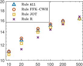
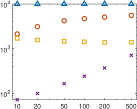
[Iteration count]    [Average $|Q|$]  [Computation time (sec)]

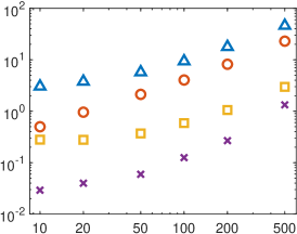
(b) Strongly convex QP: $H\succ\mathbf{0}$

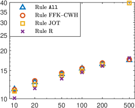
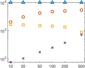
[Iteration count]    [Average $|Q|$]  [Computation time (sec)]

(c) linear optimization: $H=\mathbf{0}$

Figure 1: Randomly generated problems with $m=10\,000$ constraints– Numerical results on two types of randomly generated problems. In each figure, the $x$-axis is the number of variables ($n$) and the $y$-axis is iteration count, average size of working set, or computation time, all averaged over the 50 problem instances and plotted in logarithmic scale. The results of Rule All, Rule FFK–CWH, Rule JOT, and Rule R are plotted as blue triangles, red circles, yellow squares, and purple crosses, respectively.

It is clear from the plots that, in terms of computation time, Rule R outperforms other constraint-selection rules for the randomly generated problems we tested. When the number of variables ($n$) is $1\%\sim 5\%$ of the number of constraints ($m$) (i.e, $n$=100 to 500), Algorithm 2.2 with Rule R is two to five times faster than with the second best rule, or 20 to 50 times faster than the unreduced algorithm (Rule All). When $n$ is lowered to less than $1\%$ of $m$ (i.e., $n<100$), the time advantage of using Rule R further doubles. Note that, as $n$ decreases, Rule R is asymptotically more restrictive than Rule FFK–CWH and Rule JOT. We believe this may be the key reason that Rule R outperforms other rules, especially on problems with small $n$.

3.4 Data-Fitting Problems

We also applied Algorithm 2.2 on CQPs arising from two instances of a data-fitting problem: trigonometric curve fitting to noisy observed data points. This problem was formulated in TAW-06 as a linear optimization problem, and then in JOT-12 reformulated as a CQP by imposing a regularization term. The CQP formulation of this problem, taken from JOT-12 , is as follows. Let $g:[0,1]\to\mathbb{R}$ be a given function of time, and let $\bar{\mathbf{b}}:=[\bar{b}_{1},\dots,\bar{b}_{\bar{m}}]^{T}\in\mathbb{R}^{\bar{m}}$ be a vector that collects noisy observations of $g$ at sample time $t=t_{1},\dots,t_{\bar{m}}$. The problem aims at finding a trigonometric expansion $u(t)$ from the noisy data $\bar{\mathbf{b}}$ that best approximates $g$. Here $u(t):=\sum_{j=1}^{\bar{n}}\bar{x}_{j}\psi_{j}(t)$, with the trigonometric basis

$$\psi_{j}(t):=\begin{cases}\cos(2(j-1)\pi t)\>,&j=1,\dots,\lceil\frac{\bar{n}}{2}\rceil\\ \sin(2(j-\lceil\frac{\bar{n}}{2}\rceil)\pi t)&j=\lceil\frac{\bar{n}}{2}\rceil+1,\dots,\bar{n}\end{cases}\>.$$

Equivalently, $u(t)=\bar{A}\bar{\mathbf{x}}$, where $\bar{\mathbf{x}}:=[\bar{x}_{1},\dots,\bar{x}_{\bar{n}}]^{T}$ and $\bar{A}$ is a $\bar{m}\times\bar{n}$ matrix with entries $\bar{a}_{ij}=\psi_{j}(t_{i})$. Based on a regularized minimax approach, the problem is then formulated as

$$\operatorname*{minimize}_{\bar{\mathbf{x}}\in\mathbb{R}^{\bar{n}}}\|\bar{A}\bar{\mathbf{x}}-\bar{\mathbf{b}}\|_{\infty}+\frac{1}{2}\bar{\alpha}\bar{\mathbf{x}}^{T}\bar{H}\bar{\mathbf{x}}\>,$$

where $\bar{H}\succeq\mathbf{0}$ is a symmetric $\bar{n}\times\bar{n}$ matrix, $\bar{\alpha}$ is a regularization parameter, and $\bar{\mathbf{x}}^{T}\bar{H}\bar{\mathbf{x}}$ is a regularization term that helps resist over-fitting. This problem can be rewritten as

$$\operatorname*{minimize}_{\bar{\mathbf{x}}\in\mathbb{R}^{\bar{n}}v\in\mathbb{R}} v+\frac{1}{2}\bar{\alpha}\bar{\mathbf{x}}^{T}\bar{H}\bar{\mathbf{x}}$$

subject to $$\bar{A}\bar{\mathbf{x}}-\bar{\mathbf{b}}\geq-v\mathbf{1}\>,$$

$$- \bar{A}\bar{\mathbf{x}}+\bar{\mathbf{b}}\geq-v\mathbf{1}\>,$$

which is a CQP in the form of (P) with number of variables $n=\bar{n}+1$ and number of constraints $m=2\bar{m}$.

Following JOT-12 , we tested Algorithm 2.2 on this problem with two target functions

$$g(t)=\sin(10t)\cos(25t^{2})\quad\mbox{and}\quad g(t)=\sin(5t^{3})\cos^{2}(10t)\>.$$

In each case, as in JOT-12 , we sampled the data uniformly in time and set $\bar{b}_{i}:=g(\frac{i-1}{\bar{m}})+\epsilon_{i}$, where $\epsilon_{i}$ is an independent and identically distributed noise that takes values from $\mathcal{N}(0,0.09)$, for $i=1,\dots,\bar{m}$ and, as in JOT-12 , the regularization parameters were chosen as $\bar{\alpha}:=10^{-6}$ and $\bar{H}=\operatorname{diag}(\bar{\mathbf{h}})$, with $\bar{h}_{1}:=0$ and $\bar{h}_{j}=\bar{h}_{j+\lceil\frac{\bar{n}}{2}\rceil-1}:=2(j-1)\pi$, for $j=2,\dots,\lceil\frac{\bar{n}}{2}\rceil$, and $\bar{h}_{\bar{n}}:=2(\lfloor\frac{\bar{n}}{2}\rfloor)\pi$.

Figure 2 reports our numerical results. Since these problems involve noise, we solved the problem $50$ times for each target function and report the average results. (The average is not reported—the corresponding symbol is not plotted—for problems on which one or more of the 50 runs failed, i.e., did not converge when iteration count reaches 200.) The sizes of the tested problems are $m:=10\,000$ and $n$ ranging from 10 to 500.

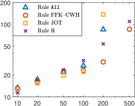
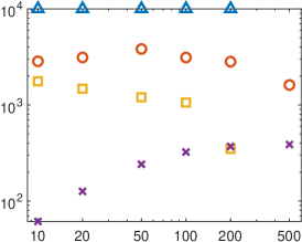
[Iteration count]    [Average $|Q|$]  [Computation time (sec)]

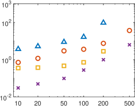
(b) $g(t)=\sin(10t)\cos(25t^{2})$

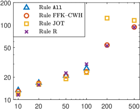
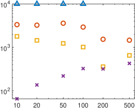
[Iteration count]    [Average $|Q|$]  [Computation time (sec)]

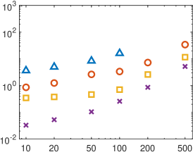
(c) $g(t)=\sin(5t^{3})\cos^{2}(10t)$

Figure 2: Data-fitting problems with $m=10\,000$ constraints – Numerical results on two data-fitting problems. In each figure, the $x$-axis is the number of variables ($n$) and the $y$-axis is iteration count, average size of working set, or computation time, all averaged over the 50 problem instances and plotted in logarithmic scale. The results of Rule All, Rule FFK–CWH, Rule JOT, and Rule R are plotted as blue triangles, red circles, yellow squares, and purple crosses, respectively.

The results show that Rule R still outperforms other constraint-selection rules in terms of computation time, especially on problems with relatively small $n$. In general, Rule R is two to ten times faster than the second best rule. We observe in Figure 2 that Rule JOT and Rule All failed to converge within $200$ iterations in a few instances on problems with relatively large $n$. Numerical results suggest that these failures are due to ill-conditioning of $M_{Q}$ apparently producing poor search directions. Thus, we conjecture that accurate identification of active constraints not only reduces computation time, but also alleviates the ill-conditioning issue of $M_{Q}$ near optimal points.

3.5 Comparison with Broadly Used, Mature Code

With a view toward calibrating the performance of Algorithm 2.2 reported in Sections 3.3 and 3.4, we carried out a numerical comparison with two widely used solvers, SDPT3 Toh-Todd-Tutuncu-1999 ; Tutuncu-Toh-Todd-2003 and SeDuMi Sturm-1999 . The tests were performed on the problems considered in Sections 3.3 and 3.4 with sizes $m=10\,000$ and $n=10,\,20,\,50,\,100,\,200,\,500$. For 2.2, the exact same implementation, including starting points and stopping criterion, as outlined in Section 3.2 was used. As for the SDPT3 and SeDuMi solvers, we set the solver precision to $10^{-8}$ and let the solvers decide the starting points.

Table 1 reports the iteration counts and computation time of SDPT3, SeDuMi, and Algorithm 2.2 with Rule All and Rule R, on each type of tested problems. The numbers in Table 1 are average values over 50 runs and over all six tested values of $n$. These results show that, for such significantly imbalanced problems, constraint reduction brings a clear edge. In particular, for such problems, Algorithm 2.2 with Rule R shows a significantly better time-performance than two mature solvers.

	Randomly generated problems				Data fitting problems
Algorithm	$H\succ\mathbf{0}$		$H=\mathbf{0}$		$\sin(10t)\cos(25t^{2})$		$\sin(5t^{3})\cos^{2}(10t)$
	iteration	time	iteration	time	iteration	time	iteration	time
SDPT3	23.6	35.8	21.2	22.3	26.2	46.1	26.7	48.7
SeDuMi	22.0	4.0	16.3	4.4	26.9	5.1	26.1	5.5
Rule All	14.1	16.5	14.7	18.7	48.8	94.3	54.3	119.4
Rule R	13.2	0.3	14.3	0.4	38.7	1.4	43.8	1.6

Table 1: Comparison of Algorithm 2.2 with popular codes – This table reports the iteration count and computation time (sec) for each of the compared algorithms on each type of tested problems, averaged over 50 runs. Every reported number is also averaged over various problems sizes: $m=10\,000$ and $n=10,\,20,\,50,\,100,\,200,\,500$.

4 Conclusion

Convergence properties of the constraint-reduced algorithm proposed in this paper, which includes a number of novelties, were proved independently of the choice of the working-set selection rule, provided the rule satisfies Condition CSR. Under a specific such rule, based on a modified active-set identification scheme, the algorithm performs remarkably well in practice, both on randomly generated problems (CQPs as well as linear optimization problems) as well as data-fitting problems.

Of course, while the focus of the present paper was on dense problems, the concept of constraint reduction also applies to imbalanced large, sparse problems. Indeed, whichever technique is used for solving the Newton-KKT system, solving instead a reduced Newton-KKT system, of like sparsity but of drastically reduced size, is bound to bring in major computational savings when the total number of inequality constraints is much larger than the number of inequality constraints that are active at the solution—at least when the number of variables is reasonably small compared to the number of inequality constraints. In the case of sparse problems, the main computation cost in an IPM iteration would be that of a (sparse) Cholesky factorization or, in an iterative approach to solving the linear system, would be linked to the number of necessary iterations for reaching needed accuracy. In both cases, a major reduction in the dimension of the Newton-KKT system is bound to reduce the computation time, and like savings as in the dense case should be expected.

Appendix

The following results are used in the proofs in Appendices A and B. Here we assume that $Q\subseteq\mathbf{m}$ and $W$ is symmetric, with $W\succeq H\succ\mathbf{0}$. First, from (10) and (13), the approximate MPC search direction $(\Delta\mathbf{x},\Delta\boldsymbol{\lambda}_{Q},\Delta\mathbf{s}_{Q})$ defined in (16) solves

$$J(W,A_{Q},\mathbf{s}_{Q},\boldsymbol{\lambda}_{Q})\left[\begin{array}[]{c}\Delta\mathbf{x}\\ \Delta\boldsymbol{\lambda}_{Q}\\ \Delta\mathbf{s}_{Q}\end{array}\right]=\left[\begin{array}[]{c}-\nabla f(\mathbf{x})+(A_{Q})^{T}\boldsymbol{\lambda}_{Q}\\ \mathbf{0}\\ -S_{Q}\boldsymbol{\lambda}_{Q}+\gamma\sigma\mu_{(Q)}\mathbf{1}-\gamma\Delta S_{Q}^{\textup{a}}\Delta\boldsymbol{\lambda}_{Q}^{\textup{a}}\end{array}\right]\>,$$ (32)

and equivalently, when $\mathbf{s}_{Q}>\mathbf{0}$, from (20), (21) and (15),

$$M_{(Q)} \Delta\mathbf{x}=-\nabla f(\mathbf{x})+(A_{Q})^{T}S_{Q}^{-1}(\gamma\sigma\mu_{(Q)}\mathbf{1}-\gamma\Delta S_{Q}^{\textup{a}}\Delta\boldsymbol{\lambda}_{Q}^{\textup{a}}),$$ (33)

$$\Delta\mathbf{s}_{Q}=A_{Q}\Delta\mathbf{x},$$

$$\Delta\boldsymbol{\lambda}_{Q}=-\boldsymbol{\lambda}_{Q}+S_{Q}^{-1}(-\Lambda_{Q}\Delta\mathbf{s}_{Q}+\gamma\sigma\mu_{(Q)}\mathbf{1}-\gamma\Delta S_{Q}^{\textup{a}}\Delta\boldsymbol{\lambda}_{Q}^{\textup{a}})\>.$$

Next, with $\tilde{\boldsymbol{\lambda}}^{+}$ and $\tilde{\boldsymbol{\lambda}}^{\textup{a},+}$ given by

$$\tilde{\lambda}^{+}_{i}:=\begin{cases}\lambda_{i}+\Delta\lambda_{i}&i\in Q,\\ 0&i\in Q^{\textup{c}},\end{cases}\quad\text{ and }\quad\tilde{\lambda}_{i}^{\textup{a},+}:=\begin{cases}\lambda_{i}+\Delta\lambda_{i}^{\textup{a}}&i\in Q,\\ 0&i\in Q^{\textup{c}},\end{cases}$$ (34)

from the last equation of (33) and from (21), we have

$$\tilde{\boldsymbol{\lambda}}_{Q}^{+}=S_{Q}^{-1}(-\Lambda_{Q}\Delta\mathbf{s}_{Q}+\gamma\sigma\mu_{(Q)}\mathbf{1}-\gamma\Delta S^{\textup{a}}_{Q}\Delta\boldsymbol{\lambda}_{Q}^{\textup{a}})\>,$$ (35)

$$\tilde{\boldsymbol{\lambda}}^{\textup{a},+}_{Q}=-S_{Q}^{-1}\Lambda_{Q}\Delta\mathbf{s}^{\textup{a}}_{Q}=-S_{Q}^{-1}\Lambda_{Q}A_{Q}\Delta\mathbf{x}^{\textup{a}}_{Q}\>,$$ (36)

and hence

$$(\Delta\mathbf{x}^{\textup{a}})^{T}(A_{Q})^{T}\tilde{\boldsymbol{\lambda}}_{Q}^{\textup{a},+}=-(\Delta\mathbf{x}^{\textup{a}})^{T}(A_{Q})^{T}S_{Q}^{-1}\Lambda_{Q}A_{Q}\Delta\mathbf{x}^{\textup{a}}\leq 0\>,$$ (37)

so that, when in addition $\boldsymbol{\lambda}>\mathbf{0}$, $(\Delta\mathbf{x}^{\textup{a}})^{T}(A_{Q})^{T}\tilde{\boldsymbol{\lambda}}^{\textup{a},+}=0$ if and only if $A_{Q}\Delta\mathbf{x}^{\textup{a}}=\mathbf{0}$. Also, (20) yields

$$\nabla f(\mathbf{x})^{T}\Delta\mathbf{x}^{\textup{a}}=-{(\Delta\mathbf{x}^{\textup{a}})}^{T}M_{(Q)}\Delta\mathbf{x}^{\textup{a}}=-{(\Delta\mathbf{x}^{\textup{a}})}^{T}W\Delta\mathbf{x}^{\textup{a}}-{(\Delta\mathbf{x}^{\textup{a}})}^{T}(A_{Q})^{T}S_{Q}^{-1}\Lambda_{Q}A_{Q}\Delta\mathbf{x}^{\textup{a}}\>.$$ (38)

Since $W\succeq H$, it follows from (37) that,

$$\nabla f(\mathbf{x})^{T}\Delta\mathbf{x}^{\textup{a}}+{(\Delta\mathbf{x}^{\textup{a}})}^{T}H\Delta\mathbf{x}^{\textup{a}}\leq 0\>.$$ (39)

In addition, when $S_{Q}\succ\mathbf{0}$, $\Lambda_{Q}\succ\mathbf{0}$ and since $W\succeq\mathbf{0}$, the right-hand side of (38) is strictly negative as long as $W\Delta\mathbf{x}^{\textup{a}}$ and $A_{Q}\Delta\mathbf{x}^{\textup{a}}$ are not both zero. In particular, when $[W~{}(A_{Q})^{T}]$ has full row rank,

$$\nabla f(\mathbf{x})^{T}\Delta\mathbf{x}^{\textup{a}}<0\quad{\rm if}~{}\Delta\mathbf{x}^{\textup{a}}\not=\mathbf{0}\>.$$ (40)

Finally, we state and prove two technical lemmas.

Lemma 3

Given an infinite index set $K$, $\{\Delta\mathbf{x}^{k}\}\to\mathbf{0}$ as $k\to\infty$, $k\in K$ if and only if $\{\Delta\mathbf{x}^{\textup{a},k}\}\to\mathbf{0}$ as $k\to\infty$, $k\in K$.

Proof

We show that $\|\Delta\mathbf{x}^{k}\|$ is sandwiched between constant multiples of $\|\Delta\mathbf{x}^{\textup{a},k}\|$. We have from the search direction given in (16) that, for all $k$, $\|\Delta\mathbf{x}^{k}-\Delta\mathbf{x}^{\textup{a},k}\|=\|\gamma\Delta\mathbf{x}^{\textup{c},k}\|\leq\tau\|\Delta\mathbf{x}^{\textup{a},k}\|$, where $\tau\in(0,1)$ and the inequality follows from (7). Apply triangle inequality leads to $(1-\tau)\|\Delta\mathbf{x}^{\textup{a},k}\|\leq\|\Delta\mathbf{x}^{k}\|\leq(1+\tau)\|\Delta\mathbf{x}^{\textup{a},k}\|$ for all $k$, proving the claim. $\Box$

Lemma 4

Suppose Assumption 9 holds. Let $Q\subset\mathbf{m}$, $\mathcal{A}\subseteq Q$, $\mathbf{x}\in\mathcal{F}_{P}^{o}$, $\mathbf{s}:=A\mathbf{x}-\mathbf{b}~{}(>\mathbf{0})$, and $\boldsymbol{\lambda}>\mathbf{0}$ enjoy the following property: With $\Delta\boldsymbol{\lambda}_{Q}$, $\Delta\boldsymbol{\lambda}^{\textup{a}}_{Q}$, $\Delta\mathbf{s}$, and $\Delta\mathbf{s}^{\textup{a}}$ produced by Iteration 2.2, $\lambda_{i}+\Delta\lambda_{i}>0$ for all $i\in\mathcal{A}$ and $s_{i}+\Delta s_{i}>0$ for all $i\in Q\setminus\mathcal{A}$. Then

$$\bar{\alpha}_{\textup{d}}\geq\min\left\{1,\,\min_{i\in Q\setminus\mathcal{A}}\left\{\frac{s_{i}}{|s_{i}+\Delta s_{i}^{\textup{a}}|}\right\},\,\min_{i\in Q\setminus\mathcal{A}}\left\{\frac{s_{i}-|\Delta s_{i}^{\textup{a}}|}{|s_{i}+\Delta s_{i}|}\right\}\right\}$$ (41)

and

$$\bar{\alpha}_{\textup{p}}\geq\min\left\{1,\,\min_{i\in\mathcal{A}}\left\{\frac{\lambda_{i}}{|\lambda_{i}+\Delta\lambda_{i}^{\textup{a}}|}\right\},\,\min_{i\in\mathcal{A}}\left\{\frac{\lambda_{i}-|\Delta\lambda_{i}^{\textup{a}}|}{|\lambda_{i}+\Delta\lambda_{i}|}\right\}\right\}\>.$$ (42)

Proof

If $\bar{\alpha}_{\textup{d}}\geq 1$, (41) holds trivially, hence suppose $\bar{\alpha}_{\textup{d}}<1$. Then, from the definition of $\bar{\alpha}_{\textup{d}}$ in (24), we know that there exists some index $i_{0}\in Q$ such that

$$\Delta\lambda_{i_{0}}<-\lambda_{i_{0}}<0\quad\text{ and }\quad\bar{\alpha}_{\textup{d}}=\frac{\lambda_{i_{0}}}{|\Delta\lambda_{i_{0}}|}\>.$$ (43)

Since $\lambda_{i}+\Delta\lambda_{i}>0$ for all $i\in\mathcal{A}$, we have $i_{0}\in Q\setminus\mathcal{A}$. Now we consider two cases: $|\Delta\lambda_{i_{0}}^{\textup{a}}|\geq|\Delta\lambda_{i_{0}}|$ and $|\Delta\lambda_{i_{0}}^{\textup{a}}|<|\Delta\lambda_{i_{0}}|$. If $|\Delta\lambda_{i_{0}}^{\textup{a}}|\geq|\Delta\lambda_{i_{0}}|$, then, since the second equation in (21) is equivalently written as $\lambda_{i}s_{i}+s_{i}\Delta\lambda_{i}^{\textup{a}}+\lambda_{i}\Delta s_{i}^{\textup{a}}=0$ for all $i\in Q$ and since $\lambda_{s}s_{i}>0$ for all $i\in\mathbf{m}$, it follows from (43) that

$$\bar{\alpha}_{\textup{d}}=\frac{\lambda_{i_{0}}}{|\Delta\lambda_{i_{0}}|}\geq\frac{\lambda_{i_{0}}}{|\Delta\lambda_{i_{0}}^{\textup{a}}|}=\frac{s_{i_{0}}}{|s_{i_{0}}+\Delta s_{i_{0}}^{\textup{a}}|}\>,$$

proving (41). To conclude, suppose now that $|\Delta\lambda_{i_{0}}^{\textup{a}}|<|\Delta\lambda_{i_{0}}|$. Since (i) $s_{i}+\Delta s_{i}>0$ for $i\in Q\setminus\mathcal{A}$; (ii) $\gamma$, $\sigma$, and $\mu_{(Q)}$ in (35) are non-negative; and (iii) $\Delta\lambda_{i_{0}}<0$ (from (43)), (34)–(35) yield

$${\lambda}_{i_{0}}(s_{i_{0}}+\Delta s_{i_{0}})\geq s_{i_{0}}|\Delta\lambda_{i_{0}}|-\gamma|\Delta s_{i_{0}}^{\textup{a}}||\Delta\lambda_{i_{0}}^{\textup{a}}|\>.$$

Applying this inequality to (43) leads to

$$\bar{\alpha}_{\textup{d}}=\frac{\lambda_{i_{0}}}{|\Delta\lambda_{i_{0}}|}\geq\frac{s_{i_{0}}}{|s_{i_{0}}+\Delta s_{i_{0}}|}-\frac{\gamma|\Delta\lambda_{i_{0}}^{\textup{a}}||\Delta s_{i_{0}}^{\textup{a}}|}{|s_{i_{0}}+\Delta s_{i_{0}}||\Delta\lambda_{i_{0}}|}\geq\frac{s_{i_{0}}-|\Delta s_{i_{0}}^{\textup{a}}|}{|s_{i_{0}}+\Delta s_{i_{0}}|},$$

where the last inequality holds since $\gamma\leq 1$ and $|\Delta\lambda_{i_{0}}^{\textup{a}}|<|\Delta\lambda_{i_{0}}|$. Following a very similar argument that flips the roles of $\mathbf{s}$ and $\boldsymbol{\lambda}$, one can prove that (42) also holds. $\Box$

Appendix A Proof of Theorem 2.1 and Corollary 12

Parts of this proof are inspired from TZ:94 , JOT-12 , JungThesis , WNTO-2012 , and WTA-2014 . Throughout, we assume that the constraint-selection rule used by the algorithm is such that Condition CSR is satisfied and (except in the proof of Lemma 13) we let $\varepsilon=0$ and assume that the iteration never stops.

A central feature of Algorithm 2.2, which plays a key role in the convergence proofs, is that it forces descent with respect of the primal objective function. The next proposition establishes some related facts.

Proposition 2

Suppose $\boldsymbol{\lambda}>\mathbf{0}$ and $\mathbf{s}>\mathbf{0}$, and $W$ satisfies $W\succ\mathbf{0}$ and $W\succeq H$. If $\Delta\mathbf{x}^{\textup{a}}\neq\mathbf{0}$, then the following inequalities hold:

$$f(\mathbf{x}+\alpha\Delta\mathbf{x}^{\textup{a}})<f(\mathbf{x})\>,\quad\forall\alpha\in(0,2)\>,$$ (44)

$$\frac{\partial}{\partial\alpha}f(\mathbf{x}+\alpha\Delta\mathbf{x}^{\textup{a}})<0\>,\quad\forall\alpha\in[0,1]\>,$$ (45)

$$f(\mathbf{x})-f(\mathbf{x}+\alpha\Delta\mathbf{x})\geq\frac{\omega}{2}(f(\mathbf{x})-f(\mathbf{x}+\alpha\Delta\mathbf{x}^{\textup{a}}))\>,\quad\forall\alpha\in[0,1]\>,$$ (46)

$$f(\mathbf{x}+\alpha\Delta\mathbf{x})<f(\mathbf{x})\>,\quad\forall\alpha\in(0,1]\>.$$ (47)

Proof

When $f(\mathbf{x}+\alpha\Delta\mathbf{x}^{\textup{a}})$ is linear in $\alpha$, i.e., when $(\Delta\mathbf{x}^{\textup{a}})^{T}H\Delta\mathbf{x}^{\textup{a}}=0$, then in view of (40), (44)–(45) hold trivially. When, on the other hand, $(\Delta\mathbf{x}^{\textup{a}})^{T}H\Delta\mathbf{x}^{\textup{a}}>0$, $f(\mathbf{x}+\alpha\Delta\mathbf{x}^{\textup{a}})$ is quadratic and strictly convex in $\alpha$ and is minimized at

$$\hat{\alpha}=-\frac{\nabla f(\mathbf{x})^{T}\Delta\mathbf{x}^{\textup{a}}}{{(\Delta\mathbf{x}^{\textup{a}})}^{T}H\Delta\mathbf{x}^{\textup{a}}}=1+\frac{{(\Delta\mathbf{x}^{\textup{a}})}^{T}\left(W-H+(A_{Q})^{T}S_{Q}^{-1}\Lambda_{Q}A_{Q}\right)\Delta\mathbf{x}^{\textup{a}}}{(\Delta\mathbf{x}^{\textup{a}})^{T}H\Delta\mathbf{x}^{\textup{a}}}\geq 1,$$

where we have used (38), (37), and the fact that $W\succeq H$, and (44)–(45) again follow. Next, note that, since $\omega>0$,

$$\psi(\theta):=\omega(f(\mathbf{x})-f(\mathbf{x}+\Delta\mathbf{x}^{\textup{a}}))-(f(\mathbf{x})-f(\mathbf{x}+\Delta\mathbf{x}^{\textup{a}}+\theta\Delta\mathbf{x}^{\textup{c}}))\>$$

is quadratic and convex. Now, since $\gamma_{1}$ satisfies the constraints in its definition (8), we see that $\psi(\gamma_{1})\leq 0$, and since $\omega\leq 1$, it follows from (44) that $\psi(0)=(\omega-1)(f(\mathbf{x})-f(\mathbf{x}+\Delta\mathbf{x}^{\textup{a}}))\leq 0$. Since $\gamma\in[0,\gamma_{1}]$ (see (7)), it follows that $\psi(\gamma)\leq 0$, i.e., since from (16) $\Delta\mathbf{x}=\Delta\mathbf{x}^{\textup{a}}+\gamma\Delta\mathbf{x}^{\textup{c}}$,

$$f(\mathbf{x})-f(\mathbf{x}+\Delta\mathbf{x})\geq\omega(f(\mathbf{x})-f(\mathbf{x}+\Delta\mathbf{x}^{\textup{a}}))\>,$$

i.e.,

$$-\nabla f(\mathbf{x})^{T}\Delta\mathbf{x}-\frac{1}{2}{\Delta\mathbf{x}}^{T}H\Delta\mathbf{x}\geq\omega\left(-\nabla f(\mathbf{x})^{T}\Delta\mathbf{x}^{\textup{a}}-\frac{1}{2}{(\Delta\mathbf{x}^{\textup{a}})}^{T}H\Delta\mathbf{x}^{\textup{a}}\right).$$ (48)

Now, for all $\alpha\in[0,1]$, invoking (48), (39), and the fact that $H\succeq\mathbf{0}$, we can write

$$f(\mathbf{x})-f(\mathbf{x}+\alpha\Delta\mathbf{x})=-\alpha\nabla f(\mathbf{x})^{T}\Delta\mathbf{x}-\frac{\alpha^{2}}{2}{\Delta\mathbf{x}}^{T}H\Delta\mathbf{x} \geq\alpha\left(-\nabla f(\mathbf{x})^{T}\Delta\mathbf{x}-\frac{1}{2}{\Delta\mathbf{x}}^{T}H\Delta\mathbf{x}\right)$$

$$\geq\omega\alpha\left(-\nabla f(\mathbf{x})^{T}\Delta\mathbf{x}^{\textup{a}}-\frac{1}{2}{(\Delta\mathbf{x}^{\textup{a}})}^{T}H\Delta\mathbf{x}^{\textup{a}}\right)$$

$$=\frac{\omega\alpha}{2}\left(-\nabla f(\mathbf{x})^{T}\Delta\mathbf{x}^{\textup{a}}-\left(\nabla f(\mathbf{x})^{T}\Delta\mathbf{x}^{\textup{a}}+{(\Delta\mathbf{x}^{\textup{a}})}^{T}H\Delta\mathbf{x}^{\textup{a}}\right)\right) \geq\frac{\alpha\omega}{2}\left(-\nabla f(\mathbf{x})^{T}\Delta\mathbf{x}^{\textup{a}}\right)$$

$$\geq\frac{\alpha\omega}{2}\left(-\nabla f(\mathbf{x})^{T}\Delta\mathbf{x}^{\textup{a}}-\frac{\alpha}{2}{(\Delta\mathbf{x}^{\textup{a}})}^{T}H\Delta\mathbf{x}^{\textup{a}}\right) =\frac{\omega}{2}(f(\mathbf{x})-f(\mathbf{x}+\alpha\Delta\mathbf{x}^{\textup{a}}))\>,$$

proving (46). Finally, since $\omega>0$, (47) is a direct consequence of (46) and (44). $\Box$

Given that the iterates are primal-feasible, an immediate consequence of Proposition 2 is that the primal sequence is bounded.

Lemma 5

Suppose Assumption 9 holds. Then $\{\mathbf{x}^{k}\}$ is bounded.

We are now ready to prove a key result, relating two successive iterates, that plays a central role in the remainder of the proof of Theorem 2.1.

Proposition 3

Suppose Assumptions 9 and 2 hold, and either $\{(\mathbf{x}^{k},\boldsymbol{\lambda}^{k})\}$ is bounded away from $\mathcal{F}^{*}$, or Assumption 3 also holds and $\{\mathbf{x}^{k}\}$ converges to the unique primal solution $\mathbf{x}^{*}$. Let $K$ be an infinite index set such that

$$\left(\inf_{k\in K}\{\chi_{k-1}\}=\right)~{}\inf\left\{\|\Delta\mathbf{x}^{\textup{a},k-1}\|^{\nu}+\|[\tilde{\boldsymbol{\lambda}}^{\textup{a},k}_{Q_{k-1}}]_{-}\|^{\nu}\colon k\in K\right\}>0\>.$$ (49)

Then $\{\Delta\mathbf{x}^{k}\}\to\mathbf{0}$ as $k\to\infty$, $k\in K$.

Proof

From Lemma 5, $\{\mathbf{x}^{k}\}$ is bounded, and hence so is $\{\mathbf{s}^{k}\}$; by construction, $\mathbf{s}^{k}$ and $\boldsymbol{\lambda}^{k}$ have positive components for all $k$, and $\{\boldsymbol{\lambda}^{k}\}$ ((26)–(27)) and $\{W_{k}\}$ are bounded. Further, for any infinite index set $K^{\prime}$ such that (49) holds, (26) and (27) imply that all components of $\{\boldsymbol{\lambda}^{k}\}$ are bounded away from zero on $K^{\prime}$. Since, in addition, $Q_{k}$ can take no more than finitely many different (set) values, it follows that there exist $\hat{\mathbf{x}}$, $\hat{\boldsymbol{\lambda}}>\mathbf{0}$, $\hat{W}\succeq\mathbf{0}$, an index set $\hat{Q}\subseteq\mathbf{m}$, and some infinite index set $\hat{K}\subseteq K^{\prime}$ such that

$$\{\mathbf{x}^{k}\} \to\hat{\mathbf{x}}\text{ as }k\to\infty\>,\>k\in\hat{K}\>,$$

$$\{\mathbf{s}^{k}\} \to\hat{\mathbf{s}}:=\{A\hat{\mathbf{x}}-\mathbf{b}\}\geq\mathbf{0}\text{ as }k\to\infty\>,\>k\in\hat{K}\>.$$ (50)

$$\{\boldsymbol{\lambda}^{k}\} \to\hat{\boldsymbol{\lambda}}>\mathbf{0}\text{ as }k\to\infty\>,\>k\in\hat{K}\>,$$ (51)

$$\{W_{k}\} \to\hat{W}\text{ as }k\to\infty\>,\>k\in\hat{K}\>,$$

$$Q_{k} =\hat{Q}\>,\>\forall k\in\hat{K}\>.$$ (52)

Next, under the stated assumptions, $J(\hat{W},A_{\hat{Q}},\hat{\mathbf{s}}_{\hat{Q}},\hat{\boldsymbol{\lambda}}_{\hat{Q}})$ is non-singular. Indeed, if $\{(\mathbf{x}^{k},\boldsymbol{\lambda}^{k})\}$ is bounded away from $\mathcal{F}^{*}$, then $E(\mathbf{x}^{k},\boldsymbol{\lambda}^{k})$ is bounded away from zero and since $H+R\succ\mathbf{0}$, $W_{k}=H+\varrho_{k}R=H+\min\left\{1,\frac{E(\mathbf{x}^{k},\boldsymbol{\lambda}^{k})}{\bar{E}}\right\}R$ is bounded away from singularity and the claim follows from Assumption 2 and Lemma 1. On the other hand, if Assumption 3 also holds and $\{\mathbf{x}^{k}\}\to\mathbf{x}^{*}$, then the claim follows from Condition CSR(ii) and Lemma 1. As a consequence of this claim, and by continuity of $J$, it follows from Newton-KKT systems (10) and (32) that there exist $\Delta\hat{\mathbf{x}}^{\textup{a}}$, $\Delta\hat{\mathbf{x}}$, $\bar{\boldsymbol{\lambda}}^{\textup{a}}_{\hat{Q}}$, $\bar{\boldsymbol{\lambda}}_{\hat{Q}}$ such that

$$\{\Delta\mathbf{x}^{\textup{a},k}\} \to\Delta\hat{\mathbf{x}}^{\textup{a}}\text{ as }k\to\infty\>,\>k\in\hat{K}\>,$$ (53)

$$\{\Delta\mathbf{x}^{k}\} \to\Delta\hat{\mathbf{x}}\text{ as }k\to\infty\>,\>k\in\hat{K}\>,$$

$$\{\Delta\mathbf{s}^{k}\} \to\Delta\hat{\mathbf{s}}:=A\Delta\hat{\mathbf{x}}\text{ as }k\to\infty\>,\>k\in\hat{K}\>,$$ (54)

$$\{\tilde{\boldsymbol{\lambda}}^{\textup{a},k+1}_{\hat{Q}}\} \to\bar{\boldsymbol{\lambda}}^{\textup{a}}_{\hat{Q}}\text{ as }k\to\infty\>,\>k\in\hat{K}\>,$$ (55)

$$\{\tilde{\boldsymbol{\lambda}}^{k+1}_{\hat{Q}}\} \to\bar{\boldsymbol{\lambda}}_{\hat{Q}}\text{ as }k\to\infty\>,\>k\in\hat{K}\>,$$ (56)

The remainder of the proof proceeds by contradiction. Thus suppose that, for the infinite index set $K$ in the statement of this lemma, $\{\Delta\mathbf{x}^{k}\}\not\to\mathbf{0}$ as $k\to\infty$, $k\in K$, i.e., for some $K^{\prime\prime}\subseteq K$, $\|\Delta\mathbf{x}^{k}\|$ is bounded away from zero on $K^{\prime\prime}$. Use $K^{\prime\prime}$ as our $K^{\prime}$ above, so that (since $\hat{K}\subseteq K^{\prime}$), $\|\Delta\mathbf{x}^{k}\|$ is bounded away from zero on $\hat{K}$. Then, in view of Lemma 3 (w.l.o.g.),

$$\inf_{k\in\hat{K}}\|\Delta\mathbf{x}^{\textup{a},k}\|>0\>.$$ (57)

In addition, we have $\mathcal{A}(\hat{\mathbf{x}})\subseteq\hat{Q}$, an implication of Condition CSR(i) when $\{(\mathbf{x}^{k},\boldsymbol{\lambda}^{k})\}$ is bounded away from $\mathcal{F}^{*}$ and of Condition CSR(ii) when Assumption 3 holds and $\{\mathbf{x}^{k}\}$ converges to $\mathbf{x}^{*}$. With these facts in hand, we next show that the sequence of primal step sizes $\{\alpha_{\textup{p}}^{k}\}$ is bounded away from zero for $k\in\hat{K}$. To this end, let us define

$$\tilde{\boldsymbol{\lambda}}^{\prime,k+1}:=-(S^{k})^{-1}\Lambda^{k}\Delta\mathbf{s}^{k}\>,\quad\forall k\>,$$ (58)

so that, for all $i\in\mathbf{m}$ and all $k$, $\tilde{\lambda}_{i}^{\prime,k+1}>0$ if and only if $\Delta s_{i}^{k}<0$, and the primal portion of (24) can be written as

$$\bar{\alpha}_{\textup{p}}^{k} :=\begin{cases}\infty&\text{if }\tilde{\boldsymbol{\lambda}}^{\prime,k+1}\leq\mathbf{0}\>,\\ \min_{i}\left\{\frac{\lambda_{i}^{k}}{\tilde{\lambda}_{i}^{\prime,k+1}}:\tilde{\lambda}_{i}^{\prime,k+1}>0\right\}&\text{otherwise.}\end{cases}$$

$$\alpha_{\textup{p}}^{k} :=\min\left\{1,\,\max\{\varkappa\bar{\alpha}_{\textup{p}},\,\bar{\alpha}_{\textup{p}}-\|\Delta\mathbf{x}^{k}\|\}\right\}\>.$$

Clearly, it is now sufficient to show that, for all $i$, $\{\tilde{\lambda}_{i}^{\prime,k+1}\}$ is bounded above on $\hat{K}$. On the one hand, this is clearly so for $i\not\in\hat{Q}$ (whence $i\not\in\mathcal{A}(\hat{\mathbf{x}})$), in view of (58) and (54), since $\{\boldsymbol{\lambda}^{k}\}$ is bounded and $\{s_{i}^{k}\}$ is bounded away from zero on $\hat{K}$ for $i\not\in\mathcal{A}(\hat{\mathbf{x}})$ (from (50)). On the other hand, in view of (52), subtracting (58) from (35) yields, for all $k\in\hat{K}$,

$$\tilde{\boldsymbol{\lambda}}^{\prime k+1}_{\hat{Q}}=\tilde{\boldsymbol{\lambda}}^{k+1}_{\hat{Q}}-\gamma_{k}\sigma_{k}\mu_{({\hat{Q}})}^{k}(S_{\hat{Q}}^{k})^{-1}\mathbf{1}+\gamma_{k}(S_{\hat{Q}}^{k})^{-1}\Delta S_{\hat{Q}}^{\textup{a},k}\Delta\boldsymbol{\lambda}_{\hat{Q}}^{\textup{a},k}\>.$$

From (56), $\{\tilde{\boldsymbol{\lambda}}^{k+1}_{\hat{Q}}\}$ is bounded on $\hat{K}$, and clearly the second term in the right-hand side of the above equation is non-positive component-wise. As for the third term, the second equation in (21) gives $(S_{Q_{k}}^{k})^{-1}\Delta S_{Q_{k}}^{\textup{a},k}=(\Lambda_{Q_{k}}^{k})^{-1}\tilde{\Lambda}_{Q_{k}}^{\textup{a},k+1}$, so that we have

$$\gamma_{k}(S_{\hat{Q}}^{k})^{-1}\Delta S_{\hat{Q}}^{\textup{a},k}\Delta\boldsymbol{\lambda}_{\hat{Q}}^{\textup{a},k}=\gamma_{k}(\Lambda_{\hat{Q}}^{k})^{-1}\tilde{\Lambda}_{\hat{Q}}^{\textup{a},k+1}\Delta\boldsymbol{\lambda}_{\hat{Q}}^{\textup{a},k}\>,\quad\forall k\in\hat{K}\>,$$

which is bounded on $\hat{K}$ since, from (51), (55), and the definition (34) of $\{\tilde{\lambda}^{\textup{a},+}\}$, both $\{\tilde{\Lambda}_{\hat{Q}}^{\textup{a},k+1}\}$ and $\{\Delta\boldsymbol{\lambda}_{\hat{Q}}^{\textup{a},k}\}$ are bounded, and from (51), $\{\boldsymbol{\lambda}^{k}_{\hat{Q}}\}$ is bounded away from zero on $\hat{K}$. Therefore, $\{\tilde{\lambda}_{i}^{\prime,k+1}\}$ is bounded above on $\hat{K}$ for $i\in\hat{Q}$ as well, proving that $\{{\alpha}_{\textup{p}}^{k}\}$ is bounded away from zero on $\hat{K}$, i.e., that there exists $\underline{\alpha}>0$ such that $\alpha_{\textup{p}}^{k}>\underline{\alpha}$, for all $k\in\hat{K}$, as claimed. Without loss of generality, choose $\underline{\alpha}$ in $(0,1)$.

Finally, we show that $\{f(\mathbf{x}^{k})\}\to-\infty$ as $k\to\infty$ on $\hat{K}$, which contradicts boundedness of $\{\mathbf{x}^{k}\}$ (Lemma 5). For all $k\in\hat{K}$, since $\Delta\mathbf{x}^{\textup{a},k}\neq\mathbf{0}$ (by (57)) and $\alpha_{\textup{p}}^{k}\in(\underline{\alpha},1]$, Proposition 2 implies that $\{f(\mathbf{x}^{k})\}$ is monotonically decreasing and that, for all $k\in\hat{K}$,

$$f(\mathbf{x}^{k}+\alpha_{\textup{p}}^{k}\Delta\mathbf{x}^{\textup{a},k})<f(\mathbf{x}^{k}+\underline{\alpha}\Delta\mathbf{x}^{\textup{a},k})\>.$$

Expanding the right-hand side yields

$$f(\mathbf{x}^{k}+\underline{\alpha}\Delta\mathbf{x}^{\textup{a},k})=f(\mathbf{x}^{k})+\underline{\alpha}\nabla f(\mathbf{x}^{k})^{T}\Delta\mathbf{x}^{\textup{a},k}+\frac{\underline{\alpha}^{2}}{2}(\Delta\mathbf{x}^{\textup{a},k})^{T}H\Delta\mathbf{x}^{\textup{a},k}$$

$$=f(\mathbf{x}^{k})+\underline{\alpha}\left(\nabla f(\mathbf{x}^{k})^{T}\Delta\mathbf{x}^{\textup{a},k}+(\Delta\mathbf{x}^{\textup{a},k})^{T}H\Delta\mathbf{x}^{\textup{a},k}\right)-\left(\underline{\alpha}-\frac{\underline{\alpha}^{2}}{2}\right)(\Delta\mathbf{x}^{\textup{a},k})^{T}H\Delta\mathbf{x}^{\textup{a},k}\>,$$

where the sum of the last two terms tends to a strictly negative limit as $k\to\infty$, $k\in\hat{K}$. Indeed, in view of (39), the second term is non-positive and (i) if $(\Delta\hat{\mathbf{x}}^{\textup{a}})^{T}H\Delta\hat{\mathbf{x}}^{\textup{a}}>0$, since $\underline{\alpha}>\underline{\alpha}^{2}/2$, from (53) and (57), the third term tends to a negative limit, and (ii) if $(\Delta\hat{\mathbf{x}}^{\textup{a}})^{T}H\Delta\hat{\mathbf{x}}^{\textup{a}}=0$ then the sum of the last two terms tends to $\underline{\alpha}\nabla f(\hat{\mathbf{x}})^{T}\Delta\hat{\mathbf{x}}^{\textup{a}}$ which is also strictly negative in view of (40), since we either have $\hat{W}\succ\mathbf{0}$ (in the case that $\{(\mathbf{x}^{k},\boldsymbol{\lambda}^{k})\}$ bounded away from $\mathcal{F}^{*}$) or at least $[\hat{W}\,(A_{\hat{Q}})^{T}]$ full row rank (in the case that Assumption 3 holds and using the fact that $\mathcal{A}(\hat{\mathbf{x}})\subseteq\hat{Q}$). It follows that, for some $\delta>0$, $f(\mathbf{x}^{k}+\alpha_{\textup{p}}^{k}\Delta\mathbf{x}^{\textup{a},k})<f(\mathbf{x}^{k})-\delta$ for all $k\in\hat{K}$ large enough. Proposition 2 (eq. (46)) then gives that $f(\mathbf{x}^{k+1}):=f(\mathbf{x}^{k}+\alpha_{\textup{p}}^{k}\Delta\mathbf{x}^{k})<f(\mathbf{x}^{k})-\frac{\omega}{2}\delta$ for all $k\in\hat{K}$ large enough, where $\omega>0$ is an algorithm parameter. Since $\{f(\mathbf{x}^{k})\}$ is monotonically decreasing, the proof is now complete. $\Box$

We now conclude the proof of Theorem 2.1 via a string of eight lemmas, each of which builds on the previous one. First, on any subsequence, if $\{\Delta\mathbf{x}^{\textup{a},k}\}$ tends to zero, then $\{\mathbf{x}^{k}\}$ approaches stationary points. (Here both $\{\tilde{\boldsymbol{\lambda}}^{\textup{a},k+1}\}$ and $\{\tilde{\boldsymbol{\lambda}}^{k+1}\}$ are as defined in (34).)

Lemma 6

Suppose that Assumption 9 holds and that $\{\mathbf{x}^{k}\}$ converges to some limit point $\hat{\mathbf{x}}$ on an infinite index set $K$. If $\{\Delta\mathbf{x}^{\textup{a},k}\}$ converges to zero on $K$, then (i) $\hat{\mathbf{x}}$ is stationary and

$$\nabla f(\mathbf{x}^{k})-\left(A_{\mathcal{A}(\hat{\mathbf{x}})}\right)^{T}\tilde{\boldsymbol{\lambda}}^{\textup{a},k+1}_{\mathcal{A}(\hat{\mathbf{x}})}\to\mathbf{0}\>,\text{ as }k\to\infty\>,\,k\in K\>.$$ (59)

If, in addition, Assumption 2 holds, then (ii) $\{\tilde{\boldsymbol{\lambda}}^{\textup{a},k+1}\}$ and $\{\tilde{\boldsymbol{\lambda}}^{k+1}\}$ converge on $K$ to $\hat{\boldsymbol{\lambda}}$, the unique multiplier associated with $\hat{\mathbf{x}}$.

Proof

Suppose $\{\mathbf{x}^{k}\}\to\hat{\mathbf{x}}$ on $K$ and $\{\Delta\mathbf{x}^{\textup{a},k}\}\to\mathbf{0}$ on $K$. Let $\mathbf{s}^{k}:=A\mathbf{x}^{k}-\mathbf{b}(>\mathbf{0})$ for all $k\in K$ and $\hat{\mathbf{s}}:=A\hat{\mathbf{x}}-\mathbf{b}(\geq\mathbf{0})$, so that $\{\mathbf{s}^{k}\}\to\hat{\mathbf{s}}$ on $K$. As a first step toward proving Claim (i), we show that, for any $i\not\in\mathcal{A}(\hat{\mathbf{x}})$, $\{\tilde{\lambda}_{i}^{\textup{a},k+1}\}\to 0$ on $K$. For $i\not\in\mathcal{A}(\hat{\mathbf{x}})$, since $\hat{s}_{i}>0$, $\{s_{i}^{k}\}$ is bounded away from zero on $K$. Since it follows from (34) and (36) that, for all $k$,

$$\tilde{\lambda}_{i}^{\textup{a},k+1}=0\>,\,\forall i\not\in Q_{k}\quad\text{and}\quad\tilde{\lambda}_{i}^{\textup{a},k+1}=-{(s_{i}^{k})}^{-1}\lambda_{i}^{k}\Delta s_{i}^{\textup{a},k}\>,\,\forall i\in Q_{k}\>,$$

and since $\{\lambda_{i}^{k}\}$ is bounded (by construction) and $\Delta\mathbf{s}^{\textup{a},k}=A\Delta\mathbf{x}^{\textup{a},k}$ (by (21)), we have $\{\tilde{\lambda}_{i}^{\textup{a},k+1}\}\to 0$ on $K$. To complete the proof of Claim (i), note that the first equation of (10) (with $H$ replaced by $W$) yields

$$\nabla f(\mathbf{x}^{k})-(A_{Q_{k}})^{T}\tilde{\boldsymbol{\lambda}}^{\textup{a},k+1}_{Q_{k}}=-W_{k}\Delta\mathbf{x}^{\textup{a},k}\>.$$

Since (i) $\{\tilde{\lambda}^{\textup{a},k+1}_{i}\}\to 0$ on $K$ for $i\not\in\mathcal{A}(\hat{\mathbf{x}})$, (ii) $\{W_{k}\}$ is bounded (since $H\preceq W_{k}\preceq H+R$), (iii) $\{\Delta\mathbf{x}^{\textup{a},k}\}\to\mathbf{0}$ on $K$, and (iv) by definition (34), $\tilde{\lambda}_{i}^{\textup{a},+}=0$ for $i\in Q^{\textup{c}}$, we conclude that (59) holds, hence $\{\left(A_{\mathcal{A}(\hat{\mathbf{x}})}\right)^{T}\tilde{\boldsymbol{\lambda}}^{\textup{a},k+1}_{\mathcal{A}(\hat{\mathbf{x}})}\}$ converges (since $\nabla f(\mathbf{x}^{k})$ does) as $k\to\infty$, $k\in K$, to a point in the range of $\left(A_{\mathcal{A}(\hat{\mathbf{x}})}\right)^{T}$, say $\left(A_{\mathcal{A}(\hat{\mathbf{x}})}\right)^{T}\hat{\boldsymbol{\lambda}}_{\mathcal{A}(\hat{\mathbf{x}})}$. We get $\nabla f(\hat{\mathbf{x}})-\left(A_{\mathcal{A}(\hat{\mathbf{x}})}\right)^{T}\hat{\boldsymbol{\lambda}}_{\mathcal{A}(\hat{\mathbf{x}})}=\mathbf{0}$, proving Claim (i). Finally, Claim (ii) follows from (59), Assumption 2, and the fact that for $i\not\in\mathcal{A}(\hat{\mathbf{x}})$, $\{\tilde{\lambda}_{i}^{\textup{a},k+1}\}\to 0$ as $k\to\infty$, $k\in K$, noting that the same argument applies to $\{\tilde{\boldsymbol{\lambda}}^{k+1}\}$, using a modified version of (59), with $\tilde{\boldsymbol{\lambda}}$ replacing $\tilde{\boldsymbol{\lambda}}^{\textup{a}}$, obtained by starting from the first equation of (32) instead of that of (10) and using the fact, proved next, that $\{\tilde{\lambda}_{i}^{k+1}\}\to 0$ on $K$ for all $i\not\in\mathcal{A}(\hat{\mathbf{x}})$. From its definition in (34) and the last equation in (33), we have that, for all $k$,

$$\tilde{\lambda}_{i}^{k+1}=0\>,\quad \forall i\not\in Q_{k}\>,$$

$$\tilde{\lambda}_{i}^{k+1}={(s_{i}^{k})}^{-1}(-\lambda_{i}^{k}\Delta s_{i}^{k}+\gamma_{k}\sigma_{k}\mu_{(Q_{k})}^{(k)}-\gamma_{k}\Delta s_{i}^{\textup{a},k}\Delta\lambda_{i}^{\textup{a},k})\>,\quad \forall i\in Q_{k}\>.$$

Since $\{\tilde{\lambda}_{i}^{\textup{a},k+1}\}$ converges (to zero) on $K$, $\{\Delta\lambda_{i}^{\textup{a},k}\}$ is bounded on $K$. Furthermore, from its definition (7)–(8) (see also (16)), $\{\gamma_{k}\}$ is bounded and $|\gamma_{k}\sigma_{k}\mu_{(Q_{k})}^{(k)}|\leq\tau\|\Delta\mathbf{x}^{\textup{a},k}\|$ for all $k$. Since $\Delta\mathbf{s}^{\textup{a},k}=A\Delta\mathbf{x}^{\textup{a},k}$ and $\Delta\mathbf{s}^{k}=A\Delta\mathbf{x}^{k}$, in view of Lemma 3, it follows that, for $i\not\in\mathcal{A}(\hat{\mathbf{x}})$, $\{\tilde{\lambda}_{i}^{k+1}\}\to 0$ on $K$. $\Box$

Lemma 6, combined with Proposition 3 via a contradiction argument, then implies that (on a subsequence), if $\{\mathbf{x}^{k}\}$ does not approach $\mathcal{F}_{P}^{*}$, then $\{\Delta\mathbf{x}^{k}\}$ approaches zero.

Lemma 7

Suppose that Assumptions 9 and 2 hold and that $\{\mathbf{x}^{k}\}$ is bounded away from $\mathcal{F}_{P}^{*}$ on some infinite index set $K$. Then $\{\Delta\mathbf{x}^{k}\}\to\mathbf{0}$ as $k\to\infty$, $k\in K$.

Proof

Proceeding by contradiction, let $K$ be an infinite index set such that $\{\mathbf{x}^{k}\}$ is bounded away from $\mathcal{F}_{P}^{*}$ on $K$ and $\{\Delta\mathbf{x}^{k}\}\not\to\mathbf{0}$ as $k\to\infty$, $k\in K$. Then, in view of Proposition 3 and boundedness of $\{\mathbf{x}^{k}\}$ (Lemma 5), there exist $\hat{Q}\subseteq\mathbf{m}$, $\hat{\mathbf{x}}\not\in\mathcal{F}_{P}^{*}$, and an infinite index set $\hat{K}\subseteq K$ such that $Q_{k}=\hat{Q}$ for all $k\in\hat{K}$ and

$$\{\mathbf{x}^{k}\}\to\hat{\mathbf{x}}\>,\text{ as }k\to\infty,\>k\in\hat{K}\>,$$

$$\{\Delta\mathbf{x}^{\textup{a},k-1}\}\to\mathbf{0}\>,\text{ as }k\to\infty,\>k\in\hat{K}\>,$$

$$\{[\tilde{\boldsymbol{\lambda}}^{\textup{a},k}_{\hat{Q}}]_{-}\}\to\mathbf{0}\>,\text{ as }k\to\infty,\>k\in\hat{K}\>.$$

On the other hand, from (25), (16) and (7)–(8),

$$\|\mathbf{x}^{k}-\mathbf{x}^{k-1}\|=\|\alpha_{\textup{p}}^{k-1}\Delta\mathbf{x}^{k-1}\|\leq\|\Delta\mathbf{x}^{k-1}\|\leq(1+\tau)\|\Delta\mathbf{x}^{\textup{a},k-1}\|\>,$$

which implies that $\{\mathbf{x}^{k-1}\}\to\hat{\mathbf{x}}$ as $k\to\infty$, $k\in\hat{K}$. It then follows from Lemma 6 that $\hat{\mathbf{x}}$ is stationary and that $[\tilde{\boldsymbol{\lambda}}^{\textup{a},k}_{\mathcal{A}(\hat{\mathbf{x}})}]_{+}$ converges to the associated multiplier vector. Hence the multipliers are non-negative, contradicting the fact that $\hat{\mathbf{x}}\not\in\mathcal{F}_{P}^{*}$. $\Box$

A contradiction argument based on Lemmas 6 and 7 then shows that $\{\mathbf{x}^{k}\}$ approaches the set of stationary points of (P).

Lemma 8

Suppose Assumptions 9 and 2 hold. Then the sequence $\{\mathbf{x}^{k}\}$ approaches the set of stationary points of (P), i.e., there exists a sequence $\{\hat{\mathbf{x}}^{k}\}$ of stationary points such that $\|\mathbf{x}^{k}-\hat{\mathbf{x}}^{k}\|$ goes to zero as $k\to\infty$.

Proof

Proceeding by contradiction, suppose the claim does not hold, i.e., (invoking Lemma 5) suppose $\{\mathbf{x}^{k}\}$ converges to some non-stationary point $\hat{\mathbf{x}}$ on some infinite index set $K$. Then $\{\Delta\mathbf{x}^{\textup{a},k}\}$ does not converge to zero on $K$ (Lemma 6(i)) and nor does $\{\Delta\mathbf{x}^{k}\}$ (Lemma 3). Since $\hat{\mathbf{x}}$ is non-stationary, this is in contradiction with Lemma 7. $\Box$

The next technical result, proved in (TZ:94, , Lemma 3.6), invokes analogues of Lemmas 5, 7 and 8.

Lemma 9

Suppose Assumptions 9 and 2 hold. Suppose $\{\mathbf{x}^{k}\}$ is bounded away from $\mathcal{F}_{P}^{*}$. Let $\hat{\mathbf{x}}$ and $\hat{\mathbf{x}}^{\prime}$ be limit points of $\{\mathbf{x}^{k}\}$ and let $\hat{\boldsymbol{\lambda}}$ and $\hat{\boldsymbol{\lambda}}^{\prime}$ be the associated KKT multipliers. Then $\hat{\boldsymbol{\lambda}}=\hat{\boldsymbol{\lambda}}^{\prime}$.

Convergence of $\{\mathbf{x}^{k}\}$ to $\mathcal{F}_{P}^{*}$ ensues, proving Claim (i) of Theorem 2.1.

Lemma 10

Suppose Assumptions 9 and 2 hold. Then $\{\mathbf{x}^{k}\}$ converges to $\mathcal{F}_{P}^{*}$.

Proof

We proceed by contradiction. Thus suppose $\{\mathbf{x}^{k}\}$ does not converge to $\mathcal{F}_{P}^{*}$. Then, since $\{\mathbf{x}^{k}\}$ is bounded (Lemma 5), (by Proposition 2) $\{f(\mathbf{x}^{k})\}$ is a bounded, monotonically decreasing sequence, and it has at least one limit point $\hat{\mathbf{x}}$ that is not in $\mathcal{F}_{P}^{*}$. Hence, $f(\hat{\mathbf{x}})=\inf_{k}f(\mathbf{x}^{k})$. Then, by Lemmas 7 and 3, $\{\Delta\mathbf{x}^{k}\}$ and $\{\Delta\mathbf{x}^{\textup{a},k}\}$ converge to zero as $k\to\infty$. It follows from Lemmas 6 and 9 that all limit points of $\{\mathbf{x}^{k}\}$ are stationary, and that both $\{\tilde{\boldsymbol{\lambda}}^{\textup{a},k}\}$ and $\{\tilde{\boldsymbol{\lambda}}^{k}\}$ converge to $\hat{\boldsymbol{\lambda}}$, the common KKT multiplier vector associated to all limit points of $\{\mathbf{x}^{k}\}$. Since $\hat{\mathbf{x}}\not\in\mathcal{F}_{P}^{*}$, there exists $i_{0}$ such that $\hat{\lambda}_{i_{0}}<0$, so that, for some $\hat{k}>0$,

$$\tilde{\lambda}_{i_{0}}^{\textup{a},k+1}<0\>\text{ and }\tilde{\lambda}_{i_{0}}^{k+1}<0\>,\quad\forall k>\hat{k}\>,$$ (60)

which, in view of Step 8 of the algorithm, implies that $i_{0}\in Q_{k}$ for all $k>\hat{k}$. Then (36) gives

$$\Delta s_{i_{0}}^{\textup{a},k}=-(\lambda_{i_{0}}^{k})^{-1}s_{i_{0}}^{k}\tilde{\lambda}_{i_{0}}^{\textup{a},k+1}\>,\quad\forall k>\hat{k}\>,$$

where $s_{i_{0}}^{k}>0$, $\lambda_{i_{0}}^{k}>0$ by construction. Thus, in view of (60), $\Delta s_{i_{0}}^{\textup{a},k}>0$ for all $k>\hat{k}$. On the other hand, the last equation of (33) gives

$$\Delta s_{i_{0}}^{k}=(\lambda_{i_{0}}^{k})^{-1}(-s_{i_{0}}^{k}\tilde{\lambda}_{i_{0}}^{k+1}+\gamma_{k}\sigma_{k}\mu_{(Q_{k})}^{k}-\gamma_{k}\Delta s_{i_{0}}^{\textup{a},k}\Delta\lambda_{i_{0}}^{\textup{a},k}),\quad\forall k>\hat{k}\>,$$ (61)

where $\gamma_{k}\geq 0$, $\sigma_{k}\geq 0$, and $\mu_{(Q_{k})}^{k}\geq 0$ by construction. Further, for $k>\hat{k}$, $\Delta\lambda_{i_{0}}^{\textup{a},k}<0$ since $\lambda_{i_{0}}^{k}>0$ and $\tilde{\lambda}_{i_{0}}^{\textup{a},k+1}(=\lambda_{i_{0}}^{k}+\Delta\lambda_{i_{0}}^{\textup{a},k})<0$. It follows that all terms in (61) are non-negative and the first term is positive, so that $\Delta s_{i_{0}}^{k}>0$ for all $k>k^{\prime}$. Moreover, for all $k>\hat{k}$, we have $s_{i_{0}}^{k+1}=s_{i_{0}}^{k}+\alpha_{\textup{p}}^{k}\Delta s_{i_{0}}^{k}>s_{i_{0}}^{k}>0$, where $\alpha_{\textup{p}}^{k}>0$ since $\mathbf{s}^{k}>\mathbf{0}$. Since $\{\mathbf{s}^{k}\}$ is bounded (Lemma 5), we then conclude that $\{s_{i_{0}}^{k}\}\to\hat{s}_{i_{0}}>0$ so that $\hat{s}_{i_{0}}\hat{\lambda}_{i_{0}}<0$, in contradiction with the stationarity of limit points. $\Box$

Under strict complementarity, the next lemma then establishes appropriate convergence of the multipliers, setting the stage for the proof of part (ii) of Theorem 2.1 in the following lemma.

Lemma 11

Suppose Assumptions 9 to 3 hold and let $(\mathbf{x}^{*},\boldsymbol{\lambda}^{*})$ be the unique primal-dual solution. Then, given any infinite index set $K$ such that $\{\Delta\mathbf{x}^{\textup{a},k}\}_{k\in K}\to\mathbf{0}$, it holds that $\{\boldsymbol{\lambda}^{k+1}\}_{k\in K}\to\boldsymbol{\xi}^{*}$, where $\xi_{i}^{*}:=\min\{\lambda^{*}_{i},\lambda^{\max}\}$, for all $i\in\mathbf{m}$.

Proof

Lemma 10 guarantees that $\{\mathbf{x}^{k}\}\to\mathbf{x}^{*}$. Let $K$ be an infinite index set such that $\{\Delta\mathbf{x}^{\textup{a},k}\}_{k\in K}\to\mathbf{0}$. Then, in view of Lemma 6(ii), $\{\tilde{\boldsymbol{\lambda}}^{\textup{a},k+1}\}_{k\in K}\to\boldsymbol{\lambda}^{*}\geq\mathbf{0}$. Accordingly, $\{\chi_{k}\}=\{\|\Delta\mathbf{x}^{\textup{a},k}\|^{\nu}+\|[\tilde{\boldsymbol{\lambda}}^{\textup{a},k+1}_{Q_{k}}]_{-}\|^{\nu}\}\to 0$ as $k\to\infty$, $k\in K$. Hence, in view of (26) and (27), the proof will be complete if we show that $\{\mathbf{\breve{\text{$\boldsymbol{\lambda}$}}}^{k+1}\}_{k\in K}\to\boldsymbol{\lambda}^{*}$, where

$$\mathbf{\breve{\text{$\lambda$}}}^{k+1}_{i}:=\lambda^{k}_{i}+\alpha_{\textup{d}}^{k}\Delta\lambda^{k}_{i}\>,\quad i\in Q_{k},\quad\mbox{and}\quad\mathbf{\breve{\text{$\lambda$}}}^{k+1}_{i}:=\mu^{k+1}_{(Q_{k})}/s_{i}^{k+1}\>,\quad i\in Q^{\textup{c}}_{k}\>,$$

or equivalently, $\{\tilde{\boldsymbol{\lambda}}^{k+1}-\mathbf{\breve{\text{$\boldsymbol{\lambda}$}}}^{k+1}\}_{k\in K}\to\mathbf{0}$, which we do now.

For every $Q\subseteq\mathbf{m}$, define the index set $K(Q):=\{k\in K:Q_{k}=Q\}$, and let $\mathcal{Q}:=\{Q\subseteq\mathbf{m}:|K(Q)|=\infty\}$. We first show that for all $Q\in\mathcal{Q}$, $\{\tilde{\boldsymbol{\lambda}}^{k+1}_{Q}-\mathbf{\breve{\text{$\boldsymbol{\lambda}$}}}^{k+1}_{Q}\}_{k\in K(Q)}\to\mathbf{0}$. For $Q\in\mathcal{Q}$, the definition (34) of $\tilde{\boldsymbol{\lambda}}^{+}$ yields

$$\|\tilde{\boldsymbol{\lambda}}^{k+1}_{Q}-\mathbf{\breve{\text{$\boldsymbol{\lambda}$}}}^{k+1}_{Q}\|=(1-\alpha_{\textup{d}}^{k})\|\Delta\boldsymbol{\lambda}^{k}_{Q}\|,\quad k\in K(Q)\>.$$

Since boundedness of $\{\boldsymbol{\lambda}^{k}_{Q}\}$ (by construction) and of $\{\tilde{\boldsymbol{\lambda}}^{k+1}_{Q}\}_{k\in K}$ (=$\{\boldsymbol{\lambda}^{k}_{Q}+\Delta\boldsymbol{\lambda}^{k}_{Q})\}_{k\in K}$) (by Lemma 6(ii)) implies boundedness of $\{\Delta\boldsymbol{\lambda}^{k}_{Q}\}_{k\in K}$, we only need $\{\alpha_{\textup{d}}^{k}\}_{k\in K(Q)}\to 1$ in order to guarantee that $\|\tilde{\boldsymbol{\lambda}}^{k+1}_{Q}-\mathbf{\breve{\text{$\boldsymbol{\lambda}$}}}^{k+1}_{Q}\|\to 0$ on $K(Q)$. Now, $\{\Delta\mathbf{x}^{\textup{a},k}\}_{k\in K}\to\mathbf{0}$ implies that $\{\Delta\mathbf{s}^{\textup{a},k}\}_{k\in K}\to\mathbf{0}$, and from Lemma 3 that $\{\Delta\mathbf{x}^{k}\}_{k\in K}\to\mathbf{0}$, implying that $\{\Delta\mathbf{s}^{k}\}_{k\in K}\to\mathbf{0}$; and $\{\mathbf{x}^{k}\}\to\mathbf{x}^{*}$ yields $\{\mathbf{s}^{k}\}\to\mathbf{s}^{*}:=A\mathbf{x}^{*}-\mathbf{b}$, so $s_{i}^{k}+\Delta s_{i}^{k}>0$ for all $i\in\mathcal{A}(\mathbf{x}^{*})^{\rm c}$, $k\in K$ large enough. Moreover, Assumption 3 gives $\lambda_{i}^{*}>0$ for all $i\in\mathcal{A}(\mathbf{x}^{*})$ so that, for sufficiently large $k\in K$, $\tilde{\lambda}_{i}^{k+1}>0$ for all $i\in\mathcal{A}(\mathbf{x}^{*})$, and Condition CSR(ii) implies that $\mathcal{A}(\mathbf{x}^{*})\subseteq Q$, so Lemma 4 applies, with $\mathcal{A}:=\mathcal{A}(\mathbf{x}^{*})$. It follows that $\{\bar{\alpha}_{\textup{d}}^{k}\}_{k\in K}\to 1$, since all terms on the right-hand side of (41) converge to one on $K$. Thus, from the definition of $\alpha_{\textup{d}}^{k}$ in (24) and the fact that $\{\Delta\mathbf{x}^{k}\}_{k\in K}\to\mathbf{0}$, we have $\{\alpha_{\textup{d}}^{k}\}_{k\in K}\to 1$ indeed, establishing that $\{\tilde{\boldsymbol{\lambda}}^{k+1}_{Q}-\mathbf{\breve{\text{$\boldsymbol{\lambda}$}}}^{k+1}_{Q}\}_{k\in K(Q)}\to\mathbf{0}$.

It remains to show that, for all $Q\in\mathcal{Q}$, $\{\tilde{\boldsymbol{\lambda}}^{k+1}_{Q^{\textup{c}}}-\mathbf{\breve{\text{$\boldsymbol{\lambda}$}}}^{k+1}_{Q^{\textup{c}}}\}_{k\in K(Q)}\to\mathbf{0}$. To show this, we first note that, since $\{\chi_{k}\}_{k\in K}\to 0$, it follows from (26) and (27) and the fact established above that $\{\mathbf{\breve{\text{$\boldsymbol{\lambda}$}}}^{k+1}_{Q}\}_{K(Q)}\to\boldsymbol{\lambda}_{Q}^{*}$ that, for all $Q\in\mathcal{Q}$,

$$\{\boldsymbol{\lambda}^{k+1}_{Q}\}\to\boldsymbol{\xi}^{*}_{Q},\quad k\to\infty,~{}k\in K(Q).$$ (62)

Next, from (26), (27), and the definition (34) of $\tilde{\boldsymbol{\lambda}}^{+}$, we have, for $Q\in\mathcal{Q}$ and sufficiently large $k\in K(Q)$,

$$|\tilde{\lambda}_{i}^{k+1}-\mathbf{\breve{\text{$\lambda$}}}_{i}^{k+1}|=\mathbf{\breve{\text{$\lambda$}}}_{i}^{k+1}=\frac{\mu_{(Q)}^{k+1}}{s_{i}^{k+1}},\quad i\in Q^{\textup{c}}\>.$$ (63)

Clearly, since $\mathcal{A}(\mathbf{x}^{*})\subseteq Q$, we have $s_{i}^{*}>0$ for $i\in Q^{\textup{c}}$. Hence, since $\{\Delta\mathbf{s}^{k}\}_{k\in K}\to\mathbf{0}$, $\{s_{i}^{k+1}\}$ is bounded away from zero on $K$ for $i\in Q^{\textup{c}}$. When $Q$ is empty, the right-hand side of (63) is set to zero (see definition (14) of $\mu_{(Q)}$). When $Q$ is not empty, since $\xi_{i}^{*}=0$ whenever $\lambda_{i}^{*}=0$, (62) and complementary slackness gives

$$\left\{\mu_{(Q)}^{k+1}\right\}=\left\{\frac{(\mathbf{s}^{k+1}_{Q})^{T}\boldsymbol{\lambda}^{k+1}_{Q}}{|Q|}\right\}\to\left\{\frac{(\mathbf{s}^{*}_{Q})^{T}\boldsymbol{\xi}^{*}_{Q}}{|Q|}\right\}=0,\quad k\in K(Q)\>,$$

and it follows from (63) that $\{\tilde{\boldsymbol{\lambda}}^{k+1}_{Q^{\textup{c}}}-\mathbf{\breve{\text{$\boldsymbol{\lambda}$}}}^{k+1}_{Q^{\textup{c}}}\}_{k\in K(Q)}\to\mathbf{0}$, completing the proof. $\Box$

Claim (ii) of Theorem 2.1 can now be proved.

Lemma 12

Suppose Assumptions 9 to 3 hold and let $(\mathbf{x}^{*},\boldsymbol{\lambda}^{*})$ be the unique primal-dual solution. Then $\{\tilde{\boldsymbol{\lambda}}^{k}\}\to\boldsymbol{\lambda}^{*}$ and $\{\boldsymbol{\lambda}^{k}\}\to\boldsymbol{\xi}^{*}$, with $\xi_{i}^{*}:=\min\{\lambda^{*}_{i},\lambda^{\max}\}$ for all $i\in\mathbf{m}$.

Proof

Again, Lemma 10 guarantees that $\{\mathbf{x}^{k}\}\to\mathbf{x}^{*}$ and $\{\mathbf{s}^{k}\}\to\mathbf{s}^{*}:=A\mathbf{x}^{*}-\mathbf{b}$. Note that if $\{\Delta\mathbf{x}^{\textup{a},k}\}\to\mathbf{0}$, the claims are immediate consequences of Lemmas 6 and 11. We now prove by contradiction that $\{\Delta\mathbf{x}^{\textup{a},k}\}\to\mathbf{0}$. Thus, suppose that for some infinite index set $K$, $\inf_{k\in K}\|\Delta\mathbf{x}^{\textup{a},k}\|>0$. Then, Lemma 3 gives $\inf_{k\in K}\|\Delta\mathbf{x}^{k}\|>0$. It follows from Proposition 3 that, on some infinite index set $K^{\prime}\subseteq K$, $\{\Delta\mathbf{x}^{\textup{a},k-1}\}\to\mathbf{0}$ and $\{[\tilde{\boldsymbol{\lambda}}^{\textup{a},k}]_{-}\}\to\mathbf{0}$. Since $Q_{k}$ is selected from a finite set and $\{W_{k}\}$ is bounded, we can assume without loss of generality that $Q_{k}=Q$ on $K^{\prime}$ for some $Q\subseteq\mathbf{m}$, and that $\{W_{k}\}\to W^{*}\succeq H$ on $K^{\prime}$. Further, from Lemma 11, $\{\boldsymbol{\lambda}^{k}\}_{k\in K^{\prime}}\to\boldsymbol{\xi}^{*}$. Therefore, $\{J(W_{k},A_{Q_{k}},\mathbf{s}_{Q_{k}},\boldsymbol{\lambda}_{Q_{k}})\}_{k\in K^{\prime}}\to J(W^{*},A_{Q},\mathbf{s}_{Q}^{*},\boldsymbol{\xi}_{Q}^{*})$, and in view of Assumptions 2 and 3 and Lemma 1, $J(W^{*},A_{Q},\mathbf{s}_{Q}^{*},\boldsymbol{\xi}_{Q}^{*})$ is non-singular (since $(\mathbf{x}^{*},\boldsymbol{\lambda}^{*})$ is optimal). It follows from (10), with $W$ substituted for $H$, that $\{\Delta\mathbf{x}^{\textup{a},k}\}\to\mathbf{0}$ on $K^{\prime}$, a contradiction, proving that $\{\Delta\mathbf{x}^{\textup{a},k}\}\to\mathbf{0}$. $\Box$

Claim (iv) of Theorem 2.1 follows as well.

Lemma 13

Suppose Assumptions 9 and 2 hold and $\varepsilon>0$. Then Algorithm 2.2 terminates (in Step 1) after finitely many iterations.

Proof

If $\{(\mathbf{x}^{k},\boldsymbol{\lambda}^{k})\}$ has a limit point in $\mathcal{F}^{*}$, then $\inf_{k}\{E_{k}\}=0$, proving the claim. Thus, suppose that $\{(\mathbf{x}^{k},\boldsymbol{\lambda}^{k})\}$ is bounded away from $\mathcal{F}^{*}$. In view of Lemmas 5 and 10, $\{\mathbf{x}^{k}\}$ has a limit point $\mathbf{x}^{*}\in\mathcal{F}_{P}^{*}$. Assumption 2 then implies that there exists a unique KKT multiplier vector $\boldsymbol{\lambda}^{*}\geq\mathbf{0}$ associated to $\mathbf{x}^{*}$. If $(\mathbf{x}^{*},\boldsymbol{\lambda}^{*})\in\mathcal{F}^{*}$ is a limit point of $\{(\mathbf{x}^{k},\tilde{\boldsymbol{\lambda}}^{k})\}$, which also implies that $\inf_{k}\{E(\mathbf{x}^{k},\tilde{\boldsymbol{\lambda}}^{k})\}=0$, then in view of the stopping criterion, the claim again follows. Thus, further suppose that there is an infinite index set $K$ such that $\{\mathbf{x}^{k}\}_{k\in K}\to\mathbf{x}^{*}$, but $\inf_{k\in K}\|\tilde{\boldsymbol{\lambda}}^{k}-\boldsymbol{\lambda}^{*}\|>0$. It then follows from Lemma 6(ii) that $\{\Delta\mathbf{x}^{\textup{a},k-1}\}_{k\in K}\not\to\mathbf{0}$, and from Lemma 3 that $\{\Delta\mathbf{x}^{k-1}\}_{k\in K}\not\to\mathbf{0}$. Proposition 3 and Lemma 3 then imply that $\{\Delta\mathbf{x}^{\textup{a},k-2}\}_{k\in K^{\prime}}\to\mathbf{0}$ and $\{\Delta\mathbf{x}^{k-2}\}_{k\in K^{\prime}}\to\mathbf{0}$ for some infinite index set $K^{\prime}\subseteq K$. Next, from Lemmas 5 and 10, we have $\{\mathbf{x}^{k-2}\}_{k\in K^{\prime\prime}}\to\mathbf{x}^{**}\in\mathcal{F}_{P}^{*}$ for some infinite index set $K^{\prime\prime}\subseteq K^{\prime}$, and in view of Lemma 6(ii) $\{\tilde{\boldsymbol{\lambda}}^{k-1}\}_{k\in K^{\prime\prime}}\to\boldsymbol{\lambda}^{**}$, where $\boldsymbol{\lambda}^{**}$ is the KKT multiplier associated to $\mathbf{x}^{**}$. Since $\alpha_{\textup{p}}^{k}\in[0,1]$ for all $k$, we also have $\{\mathbf{x}^{k-1}\}_{k\in K^{\prime\prime}}=\{\mathbf{x}^{k-2}+\alpha_{\textup{p}}^{k-2}\Delta\mathbf{x}^{k-2}\}_{k\in K^{\prime\prime}}\to\mathbf{x}^{**}$, i.e., $\{(\mathbf{x}^{k-1},\tilde{\boldsymbol{\lambda}}^{k-1})\}_{k\in K^{\prime\prime}}\to(\mathbf{x}^{**},\boldsymbol{\lambda}^{**})\in\mathcal{F}^{*}$, completing the proof. $\Box$

Proof of Theorem 2.1. Claim (i) was proved in Lemma 10 and Claim (ii) in Lemma 12, Claim (iii) is a direct consequence of Condition CSR(ii), and Claim (iv) was proved in Lemma 13.

Proof of Corollary 12. From Theorem 2.1, $\{(\mathbf{x}^{k},\boldsymbol{\lambda}^{k})\}\to(\mathbf{x}^{*},\boldsymbol{\lambda}^{*})$, i.e., $\{E_{k}\}\to 0$. It follows that (i) in view of Proposition 1 and Condition CSR(ii) $Q_{k}\supseteq\mathcal{A}(x^{*})$ for all $k$ large enough, and (ii) in view of Rule R, $\{\delta_{k}\}\to 0$, so that $Q_{k}$ eventually excludes all indexes that are not in $\mathcal{A}(\mathbf{x}^{*})$. $\Box$

Appendix B Proof of Theorem 2.2

Parts of this proof are adapted from JungThesis ; TZ:94 ; WNTO-2012 . Throughout, we assume that Assumption 3 holds (so that Assumption 9 also holds), that $\varepsilon=0$ and that the iteration never stops, and that $\lambda^{*}_{i}<\lambda^{\max}$ for all $i$.

Newton’s method plays the central role in the local analysis. The following lemma is standard or readily proved; see, e.g., (TZ:94, , Proposition 3.10).

Lemma 14

Let $\Phi\colon\mathbb{R}^{n}\to\mathbb{R}^{n}$ be twice continuously differentiable and let $\mathbf{t}^{*}\in\mathbb{R}^{n}$ such that $\Phi(\mathbf{t}^{*})=\mathbf{0}$. Suppose there exists $\rho>0$ such that $\frac{\partial\Phi}{\partial\mathbf{t}}(\mathbf{t})$ is non-singular for all $\mathbf{t}\in B(\mathbf{t}^{*},\rho)$. Define $\Delta^{\rm N}\mathbf{t}$ to be the Newton increment at $\mathbf{t}$, i.e., $\Delta^{\rm N}\mathbf{t}=-\left(\frac{\partial\Phi}{\partial\mathbf{t}}(\mathbf{t})\right)^{-1}\Phi(\mathbf{t})$. Then, given any $c>0$, there exists $c^{*}>0$ such that, for all $\mathbf{t}\in B(\mathbf{t}^{*},\rho)$, if $\mathbf{t}^{+}\in\mathbb{R}^{n}$ satisfies

$$\min\{|t_{i}^{+}-t_{i}^{*}|,|t_{i}^{+}-(t_{i}+(\Delta^{\rm N}t)_{i})|\}\leq c\,\max\{\|\Delta^{\rm N}\mathbf{t}\|^{2},\|\mathbf{t}-\mathbf{t}^{*}\|^{2}\},\quad i=1,\ldots,n\>,$$ (64)

then

$$\|\mathbf{t}^{+}-\mathbf{t}^{*}\|\leq c^{*}\|\mathbf{t}-\mathbf{t}^{*}\|^{2}\>.$$

For convenience, define $\mathbf{z}:=(\mathbf{x},\boldsymbol{\lambda})$ (as well as $\mathbf{z}^{*}:=(\mathbf{x}^{*},\boldsymbol{\lambda}^{*})$, etc.). For $\mathbf{z}\in\mathcal{F}^{o}:=\{\mathbf{z}:\mathbf{x}\in\mathcal{F}_{P}^{o},\,\boldsymbol{\lambda}>\mathbf{0}\}$, define

$$\varrho(\mathbf{z}):=\min\left\{1,\frac{E(\mathbf{x},\boldsymbol{\lambda})}{\bar{E}}\right\}\quad\mbox{and}\quad W(\mathbf{z}):=H+\varrho(\mathbf{z})R\>.\quad$$

The gist of the remainder of this appendix is to apply Lemma 14 to

$$\Phi_{Q}(\mathbf{z}):=\left[\begin{array}[]{c}H\mathbf{x}-(A_{Q})^{T}\boldsymbol{\lambda}_{Q}+\mathbf{c}\\ \Lambda_{Q}(A_{Q}\mathbf{x}-\mathbf{b}_{Q})\end{array}\right]\>,\quad Q\subseteq\mathbf{m}.$$

(Note that $\Phi_{Q}(\mathbf{z}^{*})=\mathbf{0}$.) Let $\mathbf{z}_{Q}:=(\mathbf{x},\boldsymbol{\lambda}_{Q})$, then the step taken on the $Q$ components along the search direction generated by the Algorithm 2.2 is analogously given by $\mathbf{\breve{\text{$\mathbf{z}$}}}^{+}_{Q}:=(\mathbf{x}^{+},\mathbf{\breve{\text{$\boldsymbol{\lambda}$}}}_{Q}^{+})$ with $\mathbf{\breve{\text{$\boldsymbol{\lambda}$}}}_{Q}^{+}:=\boldsymbol{\lambda}_{Q}+\alpha_{\textup{d}}\Delta\boldsymbol{\lambda}_{Q}$. The first major step of the proof is achieved by Proposition 4 below, where the focus is on $\mathbf{\breve{\text{$\mathbf{z}$}}}^{+}_{Q}$ rather than on $\mathbf{z}^{+}$. Thus we compare $\mathbf{\breve{\text{$\mathbf{z}$}}}^{+}_{Q}$, with $Q\in\mathcal{Q}^{*}$ to the $Q$ components of the (unregularized) Newton step, i.e., $\mathbf{z}_{Q}+(\Delta^{\rm N}\mathbf{z})_{Q}$. Define

$$\mathscr{A}:=\left[\begin{array}[]{cc}\alpha_{\textup{p}}I_{n}&\mathbf{0}\\ \mathbf{0}&\alpha_{\textup{d}}I_{|Q|}\end{array}\right]\>,\quad\mbox{and}\quad\alpha:=\min\{\alpha_{\textup{p}},\alpha_{\textup{d}}\}\>.$$

The difference between the CR-MPC iteration and the Newton iteration can be written as

$$\|\mathbf{\breve{\text{$\mathbf{z}$}}}^{+}_{Q}-(\mathbf{z}_{Q}+(\Delta^{\rm N}\mathbf{z})_{Q})\|$$ (65)

$$\leq\|\mathbf{\breve{\text{$\mathbf{z}$}}}^{+}_{Q}-(\mathbf{z}_{Q}+\Delta\mathbf{z}_{Q})\|+\|\Delta\mathbf{z}_{Q}-\Delta\mathbf{z}^{\textup{a}}_{Q}\|+\|\Delta\mathbf{z}^{\textup{a}}_{Q}-\Delta\mathbf{z}^{0}_{Q}\|+\|\Delta\mathbf{z}^{0}_{Q}-(\Delta^{\rm N}\mathbf{z})_{Q}\|$$

$$=\|(I-\mathscr{A})\Delta\mathbf{z}_{Q}\|+\gamma\|\Delta\mathbf{z}^{\textup{c}}_{Q}\|+\|\Delta\mathbf{z}^{\textup{a}}_{Q}-\Delta\mathbf{z}^{0}_{Q}\|+\|\Delta\mathbf{z}^{0}_{Q}-(\Delta^{\rm N}\mathbf{z})_{Q}\|$$

$$\leq(1-\alpha)\|\Delta\mathbf{z}_{Q}\|+\|\Delta\mathbf{z}^{\textup{c}}_{Q}\|+\|\Delta\mathbf{z}^{\textup{a}}_{Q}-\Delta\mathbf{z}^{0}_{Q}\|+\|\Delta\mathbf{z}^{0}_{Q}-(\Delta^{\rm N}\mathbf{z})_{Q}\|\>,$$

where $\Delta\mathbf{z}_{Q}:=(\Delta\mathbf{x},\Delta\boldsymbol{\lambda}_{Q})$, $\Delta\mathbf{z}^{\textup{a}}_{Q}:=(\Delta\mathbf{x}^{\textup{a}},\Delta\boldsymbol{\lambda}^{\textup{a}}_{Q})$, $\Delta\mathbf{z}^{\textup{c}}_{Q}:=(\Delta\mathbf{x}^{\textup{c}},\Delta\boldsymbol{\lambda}^{\textup{c}}_{Q})$, and $\Delta\mathbf{z}^{0}_{Q}$ is the (constraint-reduced) affine-scaling direction for the original (unregularized) system (so $\Delta^{\rm N}\mathbf{z}=\Delta\mathbf{z}^{0}_{\mathbf{m}}$).

Let

$$J_{a}(W,A,\mathbf{s},\boldsymbol{\lambda}):=\left[\begin{array}[]{cc}W&-A^{T}\\ \Lambda A&S\end{array}\right]\>.$$

The following readily proved lemma will be of help. (For details, see Lemmas B.15 and B.16 in JungThesis ; also Lemmas 13 and 1 in TAW-06 )

Lemma 15

Let $\mathbf{s},\boldsymbol{\lambda}\in\mathbb{R}^{m}$ and $Q\subseteq\mathbf{m}$ be arbitrary and let $W$ be symmetric, with $W\succeq H$. Then (i) $J_{a}(W,A_{Q},\mathbf{s}_{Q},\boldsymbol{\lambda}_{Q})$ is non-singular if and only if $J(W,A_{Q},\mathbf{s}_{Q},\boldsymbol{\lambda}_{Q})$ is, and (ii) if $\mathcal{A}(\mathbf{x}^{*})\subseteq Q$, then $J(W,A_{Q},\mathbf{s}_{Q}^{*},\boldsymbol{\lambda}_{Q}^{*})$ is non-singular (and so is $J_{a}(W,A_{Q},\mathbf{s}_{Q}^{*},\boldsymbol{\lambda}_{Q}^{*})$).

With $\mathbf{s}:=A\mathbf{x}-\mathbf{b}$, $J_{a}(H,A_{Q},\mathbf{s}_{Q},\boldsymbol{\lambda}_{Q})$, the system matrix for the (constraint-reduced) original (unregularized) “augmented” system, is the Jacobian of $\Phi_{Q}(\mathbf{z})$, i.e.,

$$J_{a}(H,A_{Q},\mathbf{s}_{Q},\boldsymbol{\lambda}_{Q})\Delta\mathbf{z}^{0}_{Q}=-\Phi_{Q}(\mathbf{z})\>,$$

and its regularized version $J_{a}(W(\mathbf{z}),A_{Q},\mathbf{s}_{Q},\boldsymbol{\lambda}_{Q})$ satisfies (among other systems solved by Algorithm 2.2)

$$J_{a}(W(\mathbf{z}),A_{Q},\mathbf{s}_{Q},\boldsymbol{\lambda}_{Q})\Delta\mathbf{z}^{\textup{a}}_{Q}=-\Phi_{Q}(\mathbf{z})\>.$$

Next, we verify that $J_{a}(W(\mathbf{z}),A_{Q},\mathbf{s}_{Q},\boldsymbol{\lambda}_{Q})$ is non-singular near $\mathbf{z}^{*}$ (so that $\Delta\mathbf{z}^{0}_{Q}$ and $\Delta\mathbf{z}^{\textup{a}}_{Q}$ in (65) are well defined) and establish other useful local properties. For convenience, we define

$$\mathcal{Q}^{*}:=\{Q\subseteq\mathbf{m}:\mathcal{A}(\mathbf{x}^{*})\subseteq Q\}\>.$$

and

$$\tilde{\mathbf{s}}^{+}:=\mathbf{s}+\Delta\mathbf{s},\qquad\tilde{\mathbf{s}}^{\textup{a},+}:=\mathbf{s}+\Delta\mathbf{s}^{\textup{a}}.$$

Lemma 16

Let $\epsilon^{*}:=\min\{1,\min_{i\in\mathbf{m}}(\lambda_{i}^{*}+s_{i}^{*})\}$. There exist $\rho^{*}>0$ and $r>0$, such that, for all $\mathbf{z}\in\mathcal{F}^{o}\cap B(\mathbf{z}^{*},\rho^{*})$ and all $Q\in\mathcal{Q}^{*}$, the following hold:

1. $\|J_{a}(W(\mathbf{z}),A_{Q},\boldsymbol{\lambda}_{Q},\mathbf{s}_{Q})^{-1}\|\leq r$,

2. $\max\{\|\Delta\mathbf{z}^{\textup{a}}_{Q}\|,\|\Delta\mathbf{z}_{Q}\|,\|\Delta\mathbf{s}^{\textup{a}}_{Q}\|,\|\Delta\mathbf{s}_{Q}\|\}<\epsilon^{*}/4$,

3. $\min\{\lambda_{i},\tilde{\lambda}_{i}^{\textup{a},+},\tilde{\lambda}_{i}^{+}\}>\epsilon^{*}/2,\,\forall i\in\mathcal{A}(\mathbf{x}^{*})$,
   $\max\{\lambda_{i},\tilde{\lambda}_{i}^{\textup{a},+},\tilde{\lambda}_{i}^{+}\}<\epsilon^{*}/2,\,\forall i\in\mathbf{m}\setminus\mathcal{A}(\mathbf{x}^{*})$,
   $\max\{s_{i},\tilde{s}_{i}^{\textup{a},+},\tilde{s}_{i}^{+}\}<\epsilon^{*}/2,\,\forall i\in\mathcal{A}(\mathbf{x}^{*})$,
   $\min\{s_{i},\tilde{s}_{i}^{\textup{a},+},\tilde{s}_{i}^{+}\}>\epsilon^{*}/2,\,\forall i\in\mathbf{m}\setminus\mathcal{A}(\mathbf{x}^{*})$.

4. $\tilde{\lambda}_{i}^{+}<\lambda^{\max},\,\forall i\in\mathbf{m}$.

Proof

Claim (i) follows from Lemma 15, continuity of $J_{a}(W(\mathbf{z}),A_{Q},\boldsymbol{\lambda}_{Q},\mathbf{s}_{Q})$ (and the fact that $W(\mathbf{z}^{*})=H$). Claims (ii) and (iv) follow from Claim (i), Lemma 15, continuity of the right-hand sides of (10) and (32), which are zero at the solution, definition (34) of $\tilde{\boldsymbol{\lambda}}^{+}$, and our assumption that $\lambda^{*}_{i}<\lambda^{\max}$ for all $i\in\mathbf{m}$. Claim (iii) is true due to strict complementary slackness, the definition of $\epsilon^{*}$, and Claim (ii). $\Box$

In preparation for Proposition 4, Lemmas 17–20 provide bounds on the four terms in the last line of (65). The $\rho^{*}$ used in these lemmas comes from Lemma 16. The proofs of Lemmas 17, 18, and 20 are omitted, as they are very similar to those of Lemmas A.9 and A.10 in the supplementary materials of WNTO-2012 (where an MPC algorithm for linear optimization problems is considered) and of Lemma B.19 in JungThesis (also Lemma 16 inTAW-06 ).

Lemma 17

There exists a constant $c_{1}>0$ such that, for all $\mathbf{z}\in\mathcal{F}^{o}\cap B(\mathbf{z}^{*},\rho^{*})$, and for all $Q\in\mathcal{Q}^{*}$,

$$\|\Delta\mathbf{z}^{\textup{c}}_{Q}\|\leq c_{1}\|\Delta\mathbf{z}^{\textup{a}}_{Q}\|^{2}\>.$$

Note that an upper bound on the magnitude of the MPC search direction $\Delta\mathbf{z}_{Q}$ can be obtained by using Lemma 17 and Lemma 16(ii), viz.

$$\|\Delta\mathbf{z}_{Q}\|\leq\|\Delta\mathbf{z}^{\textup{a}}_{Q}\|+\|\Delta\mathbf{z}^{\textup{c}}_{Q}\|\leq\|\Delta\mathbf{z}^{\textup{a}}_{Q}\|+c_{1}\|\Delta\mathbf{z}^{\textup{a}}_{Q}\|^{2}\leq\left(1+c_{1}\frac{\epsilon^{*}}{4}\right)\|\Delta\mathbf{z}^{\textup{a}}_{Q}\|\>.$$ (66)

This bound is used in the proofs of Lemma 18 and Proposition 4.

Lemma 18

There exists a constant $c_{2}>0$ such that, for all $\mathbf{z}\in\mathcal{F}^{o}\cap B(\mathbf{z}^{*},\rho^{*})$, and for all $Q\in\mathcal{Q}^{*}$,

$$|1-\alpha|\leq c_{2}\|\Delta\mathbf{z}^{\textup{a}}_{Q}\|\>.$$

Lemma 19

There exists a constant $c_{3}>0$ such that, for all $\mathbf{z}\in\mathcal{F}^{o}\cap B(\mathbf{z}^{*},\rho^{*})$ and all $Q\in\mathcal{Q}^{*}$,

$$\|\Delta\mathbf{z}^{\textup{a}}_{Q}-\Delta\mathbf{z}^{0}_{Q}\|\leq c_{3}\|\mathbf{z}-\mathbf{z}^{*}\|^{2}.$$

Proof

We have

$$\Delta\mathbf{z}^{\textup{a}}_{Q}-\Delta\mathbf{z}^{0}_{Q}=-(J_{a}(W(\mathbf{z}),A_{Q},\mathbf{s}_{Q},\boldsymbol{\lambda}_{Q})^{-1}-J_{a}(H,A_{Q},\mathbf{s}_{Q},\boldsymbol{\lambda}_{Q})^{-1})\Phi_{Q}(\mathbf{z})$$

so that there exist $c_{31}>0$ such that, for all $\mathbf{z}\in\mathcal{F}^{o}\cap B(\mathbf{z}^{*},\rho^{*})$ and all $Q\in\mathcal{Q}^{*}$,

$$\|\Delta\mathbf{z}^{\textup{a}}_{Q}-\Delta\mathbf{z}^{0}_{Q}\|\leq c_{31}\|W(\mathbf{z})-H\|\|\mathbf{z}-\mathbf{z}^{*}\|\>,$$

where the second inequality follows from Lemma 16(i). Since $W(\mathbf{z})-H=\varrho(\mathbf{z})R$, $|\varrho(\mathbf{z})|\leq c_{32}|E(\mathbf{z})|$, and $|E(\mathbf{z})|\leq c_{33}\|\mathbf{z}-\mathbf{z}^{*}\|$, for some $c_{32}>0$ and $c_{33}>0$, the proof is complete. $\Box$

Lemma 20

There exists a constant $c_{4}>0$ such that, for all $\mathbf{z}\in\mathcal{F}^{o}\cap B(\mathbf{z}^{*},\rho^{*})$, and for all $Q\in\mathcal{Q}^{*}$,

$$\|\Delta\mathbf{z}^{0}_{Q}-(\Delta^{\rm N}\mathbf{z})_{Q}\|\leq c_{4}\|\mathbf{z}-\mathbf{z}^{*}\|\|(\Delta^{\rm N}\mathbf{z})_{Q}\|\>.$$

With Lemmas 17–20 in hand, we return to inequality (65).

Proposition 4

There exists a constant $c_{5}>0$ such that, for all $\mathbf{z}\in\mathcal{F}^{o}\cap B(\mathbf{z}^{*},\rho^{*})$, and for all $Q\in\mathcal{Q}^{*}$,

$$\|\mathbf{\breve{\text{$\mathbf{z}$}}}^{+}_{Q}-(\mathbf{z}_{Q}+(\Delta^{\rm N}\mathbf{z})_{Q})\|\leq c_{5}\max\{\|\Delta^{\rm N}\mathbf{z}\|^{2},\|\mathbf{z}-\mathbf{z}^{*}\|^{2}\}\>.$$ (67)

Proof

Let $\mathbf{z}\in\mathcal{F}^{o}\cap B(\mathbf{z}^{*},\rho^{*})$ and $Q\in\mathcal{Q}^{*}$. It follows from (65), Lemmas 17–20, and (66) that

$$\|\mathbf{\breve{\text{$\mathbf{z}$}}}^{+}_{Q}-(\mathbf{z}_{Q}+(\Delta^{\rm N}\mathbf{z})_{Q})\| \leq(1-\alpha)\|\Delta\mathbf{z}_{Q}\|+\|\Delta\mathbf{z}^{\textup{c}}_{Q}\|+\|\Delta\mathbf{z}^{\textup{a}}_{Q}-\Delta\mathbf{z}^{0}_{Q}\|+\|\Delta\mathbf{z}^{0}_{Q}-(\Delta^{\rm N}\mathbf{z})_{Q}\|$$

$$\leq c_{2}\|\Delta\mathbf{z}^{\textup{a}}_{Q}\|\|\Delta\mathbf{z}_{Q}\|+c_{1}\|\Delta\mathbf{z}^{\textup{a}}_{Q}\|^{2}+c_{3}\|\mathbf{z}-\mathbf{z}^{*}\|^{2}+c_{4}\|\mathbf{z}-\mathbf{z}^{*}\|\|(\Delta^{\rm N}\mathbf{z})_{Q}\|$$

$$\leq\left(c_{2}\left(1+c_{1}\frac{\epsilon^{*}}{4}\right)+c_{1}\right)\|\Delta\mathbf{z}^{\textup{a}}_{Q}\|^{2}+c_{3}\|\mathbf{z}-\mathbf{z}^{*}\|^{2}+c_{4}\|\mathbf{z}-\mathbf{z}^{*}\|\|(\Delta^{\rm N}\mathbf{z})_{Q}\|\>.$$

Also, by Lemmas 19 and 20, we have

$$\|\Delta\mathbf{z}^{\textup{a}}_{Q}\| \leq\|\Delta\mathbf{z}^{\textup{a}}_{Q}-\Delta\mathbf{z}^{0}_{Q}\|+\|\Delta\mathbf{z}^{0}_{Q}-(\Delta^{\rm N}\mathbf{z})_{Q}\|+\|(\Delta^{\rm N}\mathbf{z})_{Q}\|$$ (68)

$$\leq c_{3}\|\mathbf{z}-\mathbf{z}^{*}\|^{2}+c_{4}\|\mathbf{z}-\mathbf{z}^{*}\|\|(\Delta^{\rm N}\mathbf{z})_{Q}\|+\|(\Delta^{\rm N}\mathbf{z})_{Q}\|\>.$$

The claim follows (in view of boundedness of $\mathcal{F}^{o}\cap B(\mathbf{z}^{*},\rho^{*})$). $\Box$

With Proposition 4 established, we proceed to the second major step of the proof of Theorem 2.2: to show that (67) still holds when $\mathbf{z}^{+}$ is substituted for $\mathbf{\breve{\text{$\mathbf{z}$}}}^{+}_{Q}$.

Proof of Theorem 2.2. Again, let $\rho^{*}$ be as given in Lemma 16. Let $\mathbf{z}\in\mathcal{F}^{o}\cap B(\mathbf{z}^{*},\rho^{*})$ and $Q\in\mathcal{Q}^{*}$. Let $\rho:=\rho^{*}$, $\mathbf{t}:=\mathbf{z}$, and $\mathbf{t}^{*}:=\mathbf{z}^{*}$. Then the desired q-quadratic convergence is a direct consequence of Lemma 14, provided that the condition (64) is satisfied. Hence, we now show that there exists some constant $c>0$ such that, for each $i\in\mathbf{m}$,

$$\min\{|z_{i}^{+}-z_{i}^{*}|,|z_{i}^{+}-(z_{i}+(\Delta^{\rm N}z)_{i})|\}\leq c\,\max\{\|\Delta^{\rm N}\mathbf{z}\|^{2},\|\mathbf{z}-\mathbf{z}^{*}\|^{2}\}\>.$$ (69)

As per Proposition 4, (69) holds for $i\in Q$ with $z_{i}^{+}$ replaced with $\mathbf{\breve{\text{$z$}}}_{i}^{+}$. In particular, (69) holds for the $\mathbf{x}^{+}$ components of $\mathbf{z}^{+}$. It remains to show that (69) holds for the $\boldsymbol{\lambda}^{+}$ components of $\mathbf{z}^{+}$. Firstly, for all $i\in\mathcal{A}(\mathbf{x}^{*})$, we show that $\lambda_{i}^{+}=\mathbf{\breve{\text{$\lambda$}}}_{i}^{+}$, thus (69) holds for all $\lambda^{+}_{i}$ such that $i\in\mathcal{A}(\mathbf{x}^{*})$ by Proposition 4. From the fact that $\boldsymbol{\lambda}>\mathbf{0}$ ($\mathbf{z}\in\mathcal{F}^{o}$) and Lemma 16(ii), and since $\nu\geq 2$, it follows that

$$\chi:=\|\Delta\mathbf{x}^{\textup{a}}\|^{\nu}+\|[\tilde{\boldsymbol{\lambda}}^{\textup{a},+}_{Q}]_{-}\|^{\nu}\leq\|\Delta\mathbf{x}^{\textup{a}}\|^{\nu}+\|\Delta\boldsymbol{\lambda}^{\textup{a}}_{Q}\|^{\nu}\leq 2\left(\frac{\epsilon^{*}}{4}\right)^{\nu}\leq\frac{\epsilon^{*}}{2}\>,$$ (70)

so that $\min\{\chi,\underline{\lambda}\}\leq\epsilon^{*}/2$. Also, from Lemma 16(iii) and the fact that $\mathbf{\breve{\text{$\boldsymbol{\lambda}$}}}_{Q}^{+}$ is a convex combination of $\boldsymbol{\lambda}_{Q}$ and $\tilde{\boldsymbol{\lambda}}_{Q}^{+}$, we have, for all $i\in\mathcal{A}(\mathbf{x}^{*})$,

$$\frac{\epsilon^{*}}{2}<\min\{\lambda_{i},\tilde{\lambda}_{i}^{+}\}\leq\mathbf{\breve{\text{$\lambda$}}}_{i}^{+}\>.$$ (71)

Hence, from (70), (71), Lemma 16(iv), and (26), we conclude that $\lambda_{i}^{+}=\mathbf{\breve{\text{$\lambda$}}}_{i}^{+}$ for all $i\in\mathcal{A}(\mathbf{x}^{*})$. Secondly, we prove that there exists $d_{1}>0$ such that

$$\|\boldsymbol{\lambda}_{Q\setminus\mathcal{A}(\mathbf{x}^{*})}^{+}\|=\|\boldsymbol{\lambda}_{Q\setminus\mathcal{A}(\mathbf{x}^{*})}^{+}-\boldsymbol{\lambda}_{Q\setminus\mathcal{A}(\mathbf{x}^{*})}^{*}\|\leq d_{1}\max\{\|\Delta^{\rm N}\mathbf{z}\|^{2},\|\mathbf{z}-\mathbf{z}^{*}\|^{2}\}\quad\forall i\in Q\setminus\mathcal{A}(\mathbf{x}^{*})\>,$$ (72)

thus establishing (69) for $\lambda_{i}^{+}$ with $i\in Q\setminus\mathcal{A}(\mathbf{x}^{*})$. For $i\in Q\setminus\mathcal{A}(\mathbf{x}^{*})$, we know from (26) that, either $\lambda_{i}^{+}=\min\{\lambda^{\max},\mathbf{\breve{\text{$\lambda$}}}_{i}^{+}\}$, or $\lambda_{i}^{+}=\min\{\underline{\lambda},\|\Delta\mathbf{x}^{\textup{a}}\|^{\nu}+\|[\tilde{\boldsymbol{\lambda}}^{\textup{a},+}_{Q}]_{-}\|^{\nu}\}$. In the former case, we have

$$|\lambda_{i}^{+}|\leq|\mathbf{\breve{\text{$\lambda$}}}_{i}^{+}|=|\mathbf{\breve{\text{$\lambda$}}}_{i}^{+}-\lambda_{i}^{*}| \leq|\mathbf{\breve{\text{$\lambda$}}}_{i}^{+}-(\lambda_{i}+(\Delta^{\rm N}\lambda)_{i})|+|(\lambda_{i}+(\Delta^{\rm N}\lambda)_{i})-\lambda_{i}^{*}|$$

$$\leq d_{2}\max\{\|\Delta^{\rm N}\mathbf{z}\|^{2},\|\mathbf{z}-\mathbf{z}^{*}\|^{2}\}+d_{3}\|\mathbf{z}-\mathbf{z}^{*}\|^{2}\>,$$

for some $d_{2}>0$, $d_{3}>0$. Here the last inequality follows from Proposition 4 and the quadratic rate of the Newton step given in Lemma 14. In the latter case, since $\boldsymbol{\lambda}>\mathbf{0}$, we obtain

$$|\lambda_{i}^{+}|\leq\|\Delta\mathbf{x}^{\textup{a}}\|^{\nu}+\|[[\tilde{\boldsymbol{\lambda}}^{\textup{a},+}_{Q}]_{-}\|^{\nu}\leq\|\Delta\mathbf{x}^{\textup{a}}\|^{\nu}+\|\Delta\boldsymbol{\lambda}^{\textup{a}}_{Q}\|^{\nu}=\|\Delta\mathbf{z}^{\textup{a}}_{Q}\|^{\nu}\leq d_{4}\max\{\|\Delta^{\rm N}\mathbf{z}\|^{2},\|\mathbf{z}-\mathbf{z}^{*}\|^{2}\}\>,$$ (73)

for some $d_{4}>0$. Here the equality is from the definition of $\Delta\mathbf{z}^{\textup{a}}$ and the last inequality follows from $\nu\geq 2$, (68), and boundedness of $\mathcal{F}^{o}\cap B(\mathbf{z}^{*},\rho^{*})$. Hence, we have established (72). Thirdly and finally, consider the case that $i\in Q^{\textup{c}}$. Since $\mathcal{A}(\mathbf{x}^{*})\subseteq Q$, $\boldsymbol{\lambda}_{Q^{\textup{c}}}^{*}=\mathbf{0}$ and it follows from (27) that, either $\lambda_{i}^{+}=\min\{\lambda^{\max},{\mu_{(Q)}^{+}}/{s_{i}^{+}}\}$, or $\lambda_{i}^{+}=\min\{\underline{\lambda},\|\Delta\mathbf{x}^{\textup{a}}\|^{\nu}+\|[\tilde{\boldsymbol{\lambda}}^{\textup{a}}_{Q}]_{-}\|^{\nu}\}$. In the latter case, the bound in (73) follows. In the former case, we have

$$|\lambda_{i}^{+}-\lambda_{i}^{*}|=|\lambda_{i}^{+}|\leq{\mu_{(Q)}^{+}}/{s_{i}^{+}}\>.$$

By definition, $s_{i}^{+}:=s_{i}+\alpha_{\textup{p}}\Delta s_{i}$ is a convex combination of $s_{i}$ and $\tilde{s}_{i}^{+}$. Thus, Lemma 16(iii) gives that $s_{i}^{+}\geq\min\{s_{i},\tilde{s}_{i}^{+}\}>\epsilon^{*}/2$. Then using the definition of $\mu_{(Q)}^{+}$ (see Step 10 of Algorithm 2.2) leads to

$$|\lambda_{i}^{+}-\lambda_{i}^{*}|\leq\begin{cases}\frac{2}{\epsilon^{*}|Q|}\left((\mathbf{s}_{\mathcal{A}(\mathbf{x}^{*})}^{+})^{T}(\boldsymbol{\lambda}_{\mathcal{A}(\mathbf{x}^{*})}^{+})+(\mathbf{s}_{Q\setminus\mathcal{A}(\mathbf{x}^{*})}^{+})^{T}(\boldsymbol{\lambda}_{Q\setminus\mathcal{A}(\mathbf{x}^{*})}^{+})\right),&\text{if }|Q|\neq 0\\ 0\>,&\text{otherwise}\end{cases}\>.$$

Since $\mathbf{z}\in B(\mathbf{z}^{*},\rho^{*})$, $\boldsymbol{\lambda}_{\mathcal{A}(\mathbf{x}^{*})}^{+}$ and $\mathbf{s}_{Q\setminus\mathcal{A}(\mathbf{x}^{*})}^{+}$ are bounded by Lemma 16(ii). Also, by definition, $\mathbf{s}_{\mathcal{A}(\mathbf{x}^{*})}^{*}=\mathbf{0}$. Thus there exist $d_{5}>0$ and $d_{6}>0$ such that

$$|\lambda_{i}^{+}-\lambda_{i}^{*}|\leq d_{5}\|\mathbf{s}_{\mathcal{A}(\mathbf{x}^{*})}^{+}-\mathbf{s}_{\mathcal{A}(\mathbf{x}^{*})}^{*}\|+d_{6}\|\boldsymbol{\lambda}_{Q\setminus\mathcal{A}(\mathbf{x}^{*})}^{+}\|\>.$$

Having already established that the second term is bounded by the right-hand side of (72), and we are left to prove that the first term also is. By definition,

$$\|\mathbf{s}_{\mathcal{A}(\mathbf{x}^{*})}^{+}-\mathbf{s}_{\mathcal{A}(\mathbf{x}^{*})}^{*}\|=\|A_{\mathcal{A}(\mathbf{x}^{*})}\mathbf{x}^{+}-A_{\mathcal{A}(\mathbf{x}^{*})}\mathbf{x}^{*}\|\leq\|A\mathbf{x}^{+}-A\mathbf{x}^{*}\|\leq\|A\|\|\mathbf{\breve{\text{$\mathbf{z}$}}}_{Q}^{+}-\mathbf{z}_{Q}^{*}\|\>.$$

Applying Proposition 4 and Lemma 14, we get

$$\|\mathbf{s}_{\mathcal{A}(\mathbf{x}^{*})}^{+}-\mathbf{s}_{\mathcal{A}(\mathbf{x}^{*})}^{*}\| \leq\|A\|\|\mathbf{\breve{\text{$\mathbf{z}$}}}_{Q}^{+}-(\mathbf{z}_{Q}+(\Delta^{\rm N}\mathbf{z})_{Q})\|+\|A\|\|(\mathbf{z}_{Q}+(\Delta^{\rm N}\mathbf{z})_{Q})-\mathbf{z}_{Q}^{*}\|$$

$$\leq d_{7}\max\{\|\Delta^{\rm N}\mathbf{z}\|^{2},\|\mathbf{z}-\mathbf{z}^{*}\|^{2}\}+d_{8}\|\mathbf{z}-\mathbf{z}^{*}\|^{2}\>,$$

for some $d_{7}>0$, $d_{8}>0$. Hence, we established (69) for all $i\in\mathbf{m}$, thus proving the q-quadratic convergence rate. $\Box$

References

- (1) Altman, A., Gondzio, J.: Regularized symmetric indefinite systems in interior point methods for linear and quadratic optimization. Optim. Methods Softw. 11(1-4), 275–302 (1999)
- (2) Bertsimas, D., Tsitsiklis, J.: Introduction to Linear Optimization. Athena (1997)
- (3) Cartis, C., Yan, Y.: Active-set prediction for interior point methods using controlled perturbations. Comput. Optim. Appl. 63(3), 639–684 (2016)
- (4) Castro, J., Cuesta, J.: Quadratic regularizations in an interior-point method for primal block-angular problems. Math. Prog. 130(2), 415–445 (2011)
- (5) Chen, L., Wang, Y., He, G.: A feasible active set QP-free method for nonlinear programming. SIAM J. Optimiz. 17(2), 401–429 (2006)
- (6) Dantzig, G.B., Ye, Y.: A build-up interior-point method for linear programming: Affine scaling form. Tech. rep., University of Iowa, Iowa City, IA 52242, USA (July 1991)
- (7) Drummond, L., Svaiter, B.: On well definedness of the central path. J. Optim. Theory and Appl. 102(2), 223–237 (1999)
- (8) Facchinei, F., Fischer, A., Kanzow, C.: On the accurate identification of active constraints. SIAM J Optimiz. 9(1), 14–32 (1998)
- (9) Gill, P.E., Murray, W., Ponceleón, D.B., Saunders, M.A.: Solving reduced KKT systems in barrier methods for linear programming. In: G.A. Watson, D. Griffiths (eds.) Numerical Analysis 1993, pp. 89–104. Pitman Research Notes in Mathematics 303, Longmans Press (1994)
- (10) Grant, M., Boyd, S.: Graph implementations for nonsmooth convex programs. In: V. Blondel, S. Boyd, H. Kimura (eds.) Recent Advances in Learning and Control, Lecture Notes in Control and Information Sciences, pp. 95–110. Springer-Verlag Limited (2008). http://stanford.edu/~boyd/graph_dcp.html
- (11) Grant, M., Boyd, S.: CVX: Matlab software for disciplined convex programming, Version 2.1. http://cvxr.com/cvx (2014)
- (12) Hager, W.W., Seetharama Gowda, M.: Stability in the presence of degeneracy and error estimation. Math. Prog. 85(1), 181–192 (1999)
- (13) He, M.: Infeasible constraint reduction for linear and convex quadratic optimization. Ph.D. thesis, University of Maryland (2011). URL: http://hdl.handle.net/1903/12772
- (14) He, M.Y., Tits, A.L.: Infeasible constraint-reduced interior-point methods for linear optimization. Optim. Methods Softw. 27(4-5), 801–825 (2012)
- (15) Hertog, D., Roos, C., Terlaky, T.: Adding and deleting constraints in the logarithmic barrier method for LP. In: D.Z. Du, J. Sun (eds.) Advances in Optimization and Approximation, pp. 166–185. Kluwer Academic Publishers, Dordrecht, The Netherlands (1994)
- (16) Jung, J.H.: Adaptive constraint reduction for convex quadratic programming and training support vector machines. Ph.D. thesis, University of Maryland (2008). URL: http://hdl.handle.net/1903/8020
- (17) Jung, J.H., O’Leary, D.P., Tits, A.L.: Adaptive constraint reduction for training support vector machines. Electron. T. Numer. Ana. 31, 156–177 (2008)
- (18) Jung, J.H., O’Leary, D.P., Tits, A.L.: Adaptive constraint reduction for convex quadratic programming. Comput. Optim. Appl. 51(1), 125 – 157 (2012)
- (19) Laiu, M.P.: Positive filtered PN method for linear transport equations and the associated optimization algorithm. Ph.D. thesis, University of Maryland (2016). URL: http://hdl.handle.net/1903/18732
- (20) Laiu, M.P., Hauck, C.D., McClarren, R.G., O’Leary, D.P., Tits, A.L.: Positive filtered PN moment closures for linear kinetic equations. SIAM J. Numer. Anal. 54(6), 3214–3238 (2016)
- (21) Mehrotra, S.: On the implementation of a primal-dual interior point method. SIAM J. Optim. 2(4), 575–601 (1992)
- (22) Nocedal, J., Wright, S.: Numerical Optimization. Springer Series in Operations Research and Financial Engineering. Springer New York (2006)
- (23) Park, S.: A constraint-reduced algorithm for semidefinite optimization problems with superlinear convergence. J. Optimiz. Theory App. 170(2), 512–527 (2016)
- (24) Park, S., O’Leary, D.P.: A polynomial time constraint-reduced algorithm for semidefinite optimization problems. J. Optimiz. Theory App. 166(2), 558–571 (2015)
- (25) Saunders, M.A., Tomlin, J.A.: Solving regularized linear programs using barrier methods and KKT systems. Tech. rep., SOL 96-4. Department of Operations Research, Stanford University (1996)
- (26) Sturm, J.: Using SeDuMi 1.02, a MATLAB toolbox for optimization over symmetric cones. Optim. Methods Softw. 11–12, 625–653 (1999). Version 1.05 available from http://fewcal.kub.nl/sturm
- (27) Tits, A., Wächter, A., Bakhtiari, S., Urban, T., Lawrence, C.: A primal-dual interior-point method for nonlinear programming with strong global and local convergence properties. SIAM J. Optimiz. 14(1), 173–199 (2003)
- (28) Tits, A.L., Absil, P.A., Woessner, W.P.: Constraint reduction for linear programs with many inequality constraints. SIAM J. Optimiz. 17(1), 119 – 146 (2006)
- (29) Tits, A.L., Zhou, J.L.: A simple, quadratically convergent algorithm for linear and convex quadratic programming. In: W. Hager, D. Hearn, P. Pardalos (eds.) Large Scale Optimization: State of the Art, pp. 411–427. Kluwer Academic Publishers (1994)
- (30) Toh, K.C., Todd, M.J., Tütüncü, R.H.: SDPT3 – A Matlab software package for semidefinite programming, Version 1.3. Optim. Methods Softw. 11(1-4), 545–581 (1999)
- (31) Tone, K.: An active-set strategy in an interior point method for linear programming. Math. Prog. 59(1), 345–360 (1993)
- (32) Tütüncü, R.H., Toh, K.C., Todd, M.J.: Solving semidefinite-quadratic-linear programs using SDPT3. Mathe. Prog. 95(2), 189–217 (2003)
- (33) Winternitz, L.: Primal-dual interior-point algorithms for linear programming problems with many inequality constraints. Ph.D. thesis, University of Maryland (2010). URL: http://hdl.handle.net/1903/10400
- (34) Winternitz, L.B., Nicholls, S.O., Tits, A.L., O’Leary, D.P.: A constraint-reduced variant of Mehrotra’s predictor-corrector algorithm. Comput. Optim. Appl. 51(1), 1001 – 1036 (2012)
- (35) Winternitz, L.B., Tits, A.L., Absil, P.A.: Addressing rank degeneracy in constraint-reduced interior-point methods for linear optimization. J. Optimiz. Theory App. 160(1), 127–157 (2014)
- (36) Wright, S.J.: Primal-Dual Interior-Point Methods. SIAM (1997)
- (37) Wright, S.J.: Modifying SQP for degenerate problems. SIAM J. Optimiz. 13(2), 470–497 (2002)
- (38) Ye, Y.: A “build-down” scheme for linear programming. Math. Prog. 46(1), 61–72 (1990)
- (39) Zhang, Y., Zhang, D.: On polynomiality of the Mehrotra-type predictor–corrector interior-point algorithms. Math. Prog. 68(1), 303–318 (1995)