Various methods for queue length and traffic volume estimation using probe vehicle trajectories

^aDepartment of Mechanical Engineering, University of Michigan, Ann Arbor, MI, USA

^bDidi Chuxing Inc., Beijing, China

^cDepartment of Civil and Environmental Engineering, University of Michigan, Ann Arbor, MI, USA

^dUniversity of Michigan Transportation Research Institute, University of Michigan, Ann Arbor, MI, USA

Abstract

The rapid development of connected vehicle technology and the emergence of ride-hailing services have enabled the collection of a tremendous amount of probe vehicle trajectory data. Due to the large scale, the trajectory data have become a potential substitute for the widely used fixed-location sensors in terms of the performance measures of transportation networks. Specifically, for traffic volume and queue length estimation, most of the trajectory data based methods in the existing literature either require high market penetration of the probe vehicles to identify the shockwave or require the prior information about the queue length distribution and the penetration rate, which may not be feasible in the real world. To overcome the limitations of the existing methods, this paper proposes a series of novel methods based on probability theory. By exploiting the stopping positions of the probe vehicles in the queues, the proposed methods try to establish and solve a single-variable equation for the penetration rate of the probe vehicles. Once the penetration rate is obtained, it can be used to project the total queue length and the total traffic volume. The validation results using both simulation data and real-world data show that the methods would be accurate enough for assistance in performance measures and traffic signal control at intersections, even when the penetration rate of the probe vehicles is very low.

Keywords: Probe vehicle, Queue length estimation, Penetration rate, Traffic volume estimation

1 Introduction and Motivation

Traffic volumes and queue lengths are important performance measures for signalized intersections. Conventional approaches for traffic volume measurement and queue length estimation are primarily based on fixed-location sensors, such as loop detectors (Liu et al., 2009; Lee et al., 2015; An et al., 2018). However, the installation and maintenance of the fixed-location sensors are very costly, calling for urgent needs of new alternatives of data sources. This gap can be now fulfilled, thanks to the rapid development of connected vehicle technology and the emergence of ride-hailing services. The global positioning system (GPS) devices on the connected vehicles or the smartphones in the ride-hailing vehicles could record the trajectories of these probe vehicles, providing rich information about the traffic conditions in transportation networks.

Based on the probe vehicle trajectory data, a wide range of methods have been proposed for estimating the queue lengths and traffic volumes at the signalized intersections (Guo et al., 2019). A stream of literature solves the problem from the perspective of probability theory and statistics. Comert and Cetin (2009) showed that given the penetration rate of the probe vehicles and the distribution of queue lengths, the positions of the last probe vehicles in the queues alone would be sufficient for cycle-by-cycle queue length estimation. Comert and Cetin (2009) also analyzed the relationship between the probe vehicle market penetration ratio and estimation accuracy. Comert and Cetin (2011) extended their work to both spatial and temporal dimensions by considering the time when the probe vehicles joined the queues. In 2013, Comert studied the effect of the data from stop line detection (Comert, 2013a) and proposed another simple analytical model (Comert, 2013b). Li et al. (2013) formulated the dynamics of the queue length as a state transition process and employed a Kalman filter to estimate the queue length cycle by cycle. With the assumption of Poisson distribution, Comert (2016) summarized a series of methods of queue length estimation and penetration rate estimation and evaluated the estimators systematically. As for traffic volume estimation, Zheng and Liu (2017) applied maximum likelihood estimation, assuming the vehicle arrivals at the intersections follow a time-varying Poisson process. The model was validated using the trajectory data collected from connected vehicles and taxis. Zhan et al. (2017) studied citywide traffic volume estimation using large-scale trajectory data, by combining some machine learning techniques and the traditional traffic flow theory. Wang et al. (2019) constructed a three-layer Bayesian network to capture the relationship between vehicle arrival processes and the timing information in probe vehicle trajectory data. The average arrival rate was inferred from the Bayesian network by applying the Expectation-Maximization algorithm. There is also a stream of literature that applies the shockwave theory to probe vehicle data (Ban et al., 2011; Cetin, 2012; Hao et al., 2015; Hao and Ban, 2015; Ramezani and Geroliminis, 2015; Li et al., 2017; Rompis et al., 2018), or combines probe vehicle data and loop detector data (Badillo et al., 2012; Cai et al., 2014; Wang et al., 2017; Shahrbabaki et al., 2018), to estimate or predict the queue lengths. Since these studies are not closely related to this paper methodologically, they will not be introduced in detail.

Most of the existing literature introduced above on queue length estimation focuses on cycle-by-cycle estimation and requires the prior information about the penetration rate of the probe vehicles and the distribution of queue lengths. However, the prior information is usually not available. Although a recent study by Wong et al. (2019a) proposed a novel method that provides an unbiased estimator for the probe vehicle penetration rate solely based on probe vehicle trajectory data, the method cannot handle the cases when some of the queues are empty. As for traffic volume estimation, the model developed by Zheng and Liu (2017) assumes the vehicle arrivals in each cycle follow a time-varying Poisson process, which might not be reasonable in over-saturation cases when the arrival process, the queueing process, and the departure process are all different. Although the method proposed by Zhan et al. (2017) can be applied in large scale, it requires the ground-truth traffic volume data on some road segments to build a connection between their high-level features and the actual volume categories, which implies that the method depends on not only the trajectory data but also other sources of data. Zhao et al. (2019) proposed a simplified method of finding the penetration rate of the probe vehicles based on Bayes’ theorem. Extending the method in Zhao et al. (2019), this paper aims to propose a general framework and a series of methods that can estimate queue length and traffic volume both accurately and efficiently.

Estimating the states of the whole population from a small portion of it (Wong and Wong, 2015, 2016a), in nature, has to build a connection between the small portion and the whole population by their common features. When the traffic is flowing, it is difficult to infer how many regular vehicles are around the probe vehicles. Consequently, it is almost impossible to estimate the penetration rate of the probe vehicles in the traffic. However, when the vehicles are stopping at the intersections, because the empirical value of the space headway is usually around 7.5 m/veh, the number of vehicles in front of the last probe vehicle can be roughly inferred. Although the number of vehicles behind the last probe vehicle is still unknown, the incomplete information could still provide an opportunity to estimate the penetration rate of the probe vehicles. According to the penetration rate, the total queue length and the total traffic volume can be projected by scaling up the number of probe vehicles in the queues and in the traffic, respectively (Wong and Wong, 2016b; Wong et al., 2019b). The proposed methods in this paper take the stopping positions at the intersections as the common characteristics between the probe vehicles and the regular vehicles. Since the proposed methods in this paper have few external dependencies, they could overcome the limitations of the existing methods and be applied to a broader range of scenarios. The methods have been validated by both simulation and large-scale real-world data, showing good accuracy.

The rest of this paper is organized as follows. In Section 2, a detailed description of the problem will be given. Depending upon the existence of the probe vehicles, the queues over different cycles will be categorized into two classes: the observable queues (with probe vehicles) and the hidden queues (without probe vehicles). It will also be shown that the total traffic volume and the total queue length can be easily obtained once the probe vehicle penetration rate is known. Section 3 will present four different estimators of the total length of the observable queues. Section 4 will present two different estimators of the total length of the hidden queues. In Section 5, two methods for estimating the penetration rate of the probe vehicles will be proposed, which combine the various estimators presented in Section 3 and Section 4. The proposed methods are validated and evaluated in Section 6. Finally, there will be some concluding remarks in Section 7.

2 Problem Statement

When the vehicles are stopping at the intersections due to the traffic lights, some vehicles in the queue might be the probe vehicles of which the trajectories could be recorded by the onboard GPS devices. For a specific movement and a specific time slot, the vehicle arrival process is assumed to be stationary; the probe vehicles are assumed to be homogeneously mixed with other vehicles. Let $p$ denote the penetration rate of the probe vehicles, that is, when arbitrarily selecting a vehicle from the queue, its probability of being a probe vehicle is $p$, where $p\in(0,1)$.

Suppose the trajectory data of the probe vehicles are collected for $C$ cycles. In each cycle, the positions of the probe vehicles in the queue can be easily extracted from the trajectory data. The average space headway when vehicles are stopping at the intersections is assumed to be known empirically, which is a common assumption in the relevant literature. Then, with the knowledge of the position of the stop bar, the number of vehicles in front of the last probe vehicle can also be inferred, although the number of vehicles behind the last probe vehicle is still unknown. Denote the queue length in the $i$th cycle by a random variable $Q_{i},\forall i\in\{1,2,\dots,C\}$. Denote the number of probe vehicles in the $i$th cycle by a random variable $N_{i}$. Denote the observed partial queue in the $i$th cycle by a tuple $q_{i}$ consisting of “0”s and “1”s which represent regular vehicles and probe vehicles, respectively. Denote the length of the observed partial queue by $\left|q_{i}\right|$. Apparently, $Q_{i}\geq\left|q_{i}\right|\geq N_{i},\forall i\in\{1,2,\dots,C\}$.

Figure 1 illustrates what can be easily inferred from the trajectory data. $Q_{1}$, $Q_{2}$, $Q_{4}$, $Q_{5}$, $Q_{7}$, and $Q_{9}$ are (partially) observable because of the probe vehicles in the queues. $Q_{3}$, $Q_{6}$, and $Q_{8}$ are hidden because there are no probe vehicles. Denote the total length of the observable queues and the total length of the hidden queues by $Q^{obs}$ and $Q^{hid}$, respectively. In Figure 1, $Q^{obs}=Q_{1}+Q_{2}+Q_{4}+Q_{5}+Q_{7}+Q_{9}=30$ and $Q^{hid}=Q_{3}+Q_{6}+Q_{8}=7$. In the $i$th cycle, if the queue is observable, then denote the positions of the first and the last probe vehicles by $S_{i}$ and $T_{i}$, respectively.

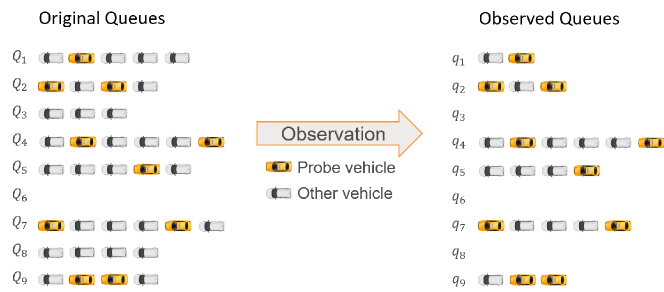
Figure 1: Observation process

Define a binary random variable $X_{i}^{l}$ to indicate if the queue length in the $i$th cycle is $l$, that is,

$$X_{i}^{l}=\begin{cases}1,&Q_{i}=l\\ 0,&Q_{i}\neq l\end{cases},$$ (1)

where $l\in\left\{0,1,\dots,L_{max}\right\}$ and $L_{max}$ is an upper bound of the queue length. Denote the number of queues of length $l$ in all the cycles by $C_{l}$. Obviously, $C=\sum_{l=0}^{L_{max}}C_{l}$ and $C_{l}=\sum_{i=1}^{C}X_{i}^{l}$.

To estimate the traffic volume and the total queue length for a specific movement and a specific time slot, the key step is to find the penetration rate $p$. Denote the total number of probe vehicles in the queues by $Q^{probe}$ and denote the traffic volume of probe vehicles by $V^{probe}$. Since $Q^{probe}$ and $V^{probe}$ can be easily obtained from the trajectory data by counting the number of probe vehicles in the queues and in the traffic flows, once $p$ is known, equation (2) and equation (3) can give an estimate of the total queue length and the total traffic volume, respectively (Wong et al., 2019b; Wong and Wong, 2019; Zhao et al., 2019).

$$\hat{Q}^{all}=\frac{Q^{probe}}{p}.$$ (2)

$$\hat{V}^{all}=\frac{V^{probe}}{p}.$$ (3)

Table 1 summarizes the notations defined above.

Table 1: Notations

Notation	Description
$C$	The total number of cycles
$Q_{i}$	The queue length in the $i$th cycle
$q_{i}$	The observed partial queue in the $i$th cycle
$N_{i}$	The number of probe vehicles in the $i$th cycle
$S_{i}$	The position of the first probe vehicle in the $i$th cycle
$T_{i}$	The position of the last probe vehicle in the $i$th cycle
$X_{i}^{l}$	A binary variable to indicate if the queue length in the $i$th cycle is $l$
$C_{l}$	The total number of queues of length $l$
$L_{max}$	An upper bound of the queue length
$Q^{obs}$	The total length of all the (partially) observable queues
$Q^{hid}$	The total length of the hidden queues
$Q^{probe}$	The total number of probe vehicles in all the queues
$V^{probe}$	The traffic volume of probe vehicles

3 Estimation of $Q^{obs}$

$Q^{obs}$ can be estimated through two approaches. Estimator 1, 2, and 3 are based on the fact that the probe vehicles are expected to segregate the regular vehicles equally. These estimators only require the number of stopping probe vehicles in each cycle and the stopping positions of the first and the last probe vehicles in the queues, all of which can be easily extracted from the trajectory data. Therefore, the estimators are constant values. By contrast, estimator 4 is based on Bayes’ theorem, which relies on the penetration rate $p$. Thus, estimator 4 is a function of $p$.

3.1 Estimator 1 using the first probe vehicles in the queues

Theorem

1:

For any integer $n_{i}\geq 1$, given that $N_{i}=n_{i}$ in the $i$th cycle,

$$\mathbb{E}(Q_{i}\mid N_{i}=n_{i})=\mathbb{E}(S_{i}\mid N_{i}=n_{i})(n_{i}+1)-1.$$ (4)

The proof is in Appendix A.

Theorem 1 states that given the number of probe vehicles in an observable queue, the expected queue length can be obtained from the expected stopping position of the first probe vehicle. Based on Theorem 1, given the number of probe vehicles in each cycle, the expected total length of the observable queues can be expressed as

$$\sum_{i:n_{i}\neq 0}\mathbb{E}(Q_{i}\mid N_{i}=n_{i}) =\sum_{i:n_{i}\neq 0}\left(\mathbb{E}\left(S_{i}\mid N_{i}=n_{i}\right)\left(n_{i}+1\right)-1\right).$$ (5)

$$=\sum_{i:n_{i}\neq 0}\mathbb{E}\left(S_{i}\mid N_{i}=n_{i}\right)\left(n_{i}+1\right)-\sum_{i:n_{i}\neq 0}1$$ (6)

$$=\sum_{j=1}^{L_{max}}\sum_{i:n_{i}=j}\mathbb{E}\left(S_{i}\mid N_{i}=j\right)\left(j+1\right)-\sum_{i:n_{i}\neq 0}1$$ (7)

$$=\sum_{j=1}^{L_{max}}\left(j+1\right)\sum_{i:n_{i}=j}\mathbb{E}\left(S_{i}\mid N_{i}=j\right)-\sum_{i:n_{i}\neq 0}1.$$ (8)

Therefore, given the position of the first stopping probe vehicle $S_{i}=s_{i}$ in the $i$th cycle, $\forall i\in\{1,2,,\dots,C\}$, by substituting the sample mean $\frac{\sum_{i:n_{i}=j}s_{i}}{\sum_{i:n_{i}=j}1}$ for the expected value $\mathbb{E}\left(S_{i}\mid N_{i}=j\right),\forall j\geq 1$, $Q^{obs}$ can be estimated by

$$\hat{Q}_{1}^{obs} =\sum_{j=1}^{L_{max}}\left(j+1\right)\sum_{i:n_{i}=j}s_{i}-\sum_{i:n_{i}\neq 0}1$$ (9)

$$=\sum_{j=1}^{L_{max}}\sum_{i:n_{i}=j}s_{i}\left(j+1\right)-\sum_{i:n_{i}\neq 0}1$$ (10)

$$=\sum_{i:n_{i}\neq 0}s_{i}\left(n_{i}+1\right)-\sum_{i:n_{i}\neq 0}1$$ (11)

$$=\sum_{i:n_{i}\neq 0}\left(s_{i}\left(n_{i}+1\right)-1\right).$$ (12)

3.2 Estimator 2 using the last probe vehicles in the queues

Theorem

2:

For any integer $n_{i}\geq 1$, given that $N_{i}=n_{i}$ in the $i$th cycle,

$$\mathbb{E}(Q_{i}\mid N_{i}=n_{i})=\mathbb{E}(T_{i}\mid N_{i}=n_{i})\frac{n_{i}+1}{n_{i}}-1.$$ (13)

The proof is in Appendix A.

Theorem 2 states that given the number of probe vehicles in an observable queue, the expected queue length can be obtained from the expected stopping position of the last probe vehicle. Based on Theorem 2, given the number of probe vehicles in each cycle, the expected total length of observable queues can be expressed as

$$\sum_{i:n_{i}\neq 0}\mathbb{E}(Q_{i}\mid N_{i}=n_{i})=\sum_{i:n_{i}\neq 0}\left(\mathbb{E}(T_{i}\mid N_{i}=n_{i})\frac{n_{i}+1}{n_{i}}-1\right).$$ (14)

Following the similar derivations with estimator 1, given the position of the last stopping probe vehicle $T_{i}=t_{i}$ in the $i$th cycle, $\forall i\in\{1,2,\dots,C\}$, by substituting the sample mean $\frac{\sum_{i:n_{i}=j}t_{i}}{\sum_{i:n_{i}=j}1}$ for the expected value $\mathbb{E}\left(T_{i}\mid N_{i}=j\right),\forall j\geq 1$, $Q^{obs}$ can be estimated by

$$\hat{Q}_{2}^{obs}=\sum_{i:n_{i}\neq 0}\left(t_{i}\frac{n_{i}+1}{n_{i}}-1\right).$$ (15)

3.3 Estimator 3 using the first and the last probe vehicles in the queues

Theorem

3:

For any integer $n_{i}\geq 1$, given that $N_{i}=n_{i}$ in the $i$th cycle,

$$\mathbb{E}(Q_{i}\mid N_{i}=n_{i})=\mathbb{E}(S_{i}\mid N_{i}=n_{i})+\mathbb{E}(T_{i}\mid N_{i}=n_{i})-1,$$ (16)

$$\mathbb{E}(Q_{i}\mid N_{i}\geq 1)=\mathbb{E}(S_{i}\mid N_{i}\geq 1)+\mathbb{E}(T_{i}\mid N_{i}\geq 1)-1.$$ (17)

The proof is in Appendix A.

Theorem 3 states that given the number of probe vehicles in an observable queue, the expected queue length can be obtained from the expected stopping positions of the first and the last probe vehicles. Based on Theorem 3, given the number of probe vehicles in each cycle, the expected total length of the observable queues can be expressed as

$$\sum_{i:n_{i}\neq 0}\mathbb{E}(Q_{i}\mid N_{i}=n_{i})=\sum_{i:n_{i}\neq 0}\left(\mathbb{E}(S_{i}\mid N_{i}=n_{i})+\mathbb{E}(T_{i}\mid N_{i}=n_{i})-1\right).$$ (18)

Therefore, by substituting the sample means $\frac{\sum_{i:n_{i}=j}s_{i}}{\sum_{i:n_{i}=j}1}$ and $\frac{\sum_{i:n_{i}=j}t_{i}}{\sum_{i:n_{i}=j}1}$ for the expected values $\mathbb{E}(S_{i}\mid N_{i}=n_{i})$ and $\mathbb{E}(T_{i}\mid N_{i}=n_{i}),\forall j\geq 1$, respectively, $Q^{obs}$ can be estimated by

$$\hat{Q}_{3}^{obs}=\sum_{i:n_{i}\neq 0}\left(s_{i}+t_{i}-1\right).$$ (19)

The mechanism behind $\hat{Q}_{3}^{obs}$ is intuitive. Take Figure 2 for example. The queue in the $k$th cycle is the reverse of the queue in the $j$th cycle, which implies that the number of vehicles behind the last probe vehicle in the $j$th cycle is equal to the number of vehicles in front of the first probe vehicle in the $k$th cycle. Because of the symmetry, these two queues have the same probability of occurring. Therefore, even though the number of vehicles behind the last probe vehicle in a cycle is unknown, as long as the sample size is sufficient, the missing number could be compensated by the number of vehicles in front of the first probe vehicle in another cycle. Essentially, $\hat{Q}_{3}^{obs}$ is obtained by summing up the position of the last probe vehicle $t_{i}$ and the number of vehicles in front of the first probe vehicle $s_{i}-1$, which could be regarded as a compensation of the missing vehicles in the rear.

Figure 2: The missing information compensated by another queue

3.4 Estimator 4 based on Bayes’ theorem

Given all the observed partial queues, as derived in Zhao et al. (2019), the conditional expectation of the total length of the observable queues can be expressed as

$$\sum_{i:n_{i}\neq 0}\mathbb{E}(Q_{i}\mid q_{i}) =\sum_{i:n_{i}\neq 0}\sum_{l=1}^{L_{max}}\frac{P(Q_{i}=l)P(q_{i}\mid Q_{i}=l)}{\sum_{j=0}^{L_{max}}P(Q_{i}=j)P(q_{i}\mid Q_{i}=j)}l$$ (20)

$$=\sum_{i:n_{i}\neq 0}\sum_{l=\left|q_{i}\right|}^{L_{max}}\frac{\mathbb{E}(C_{l})p^{n_{i}}\left(1-p\right)^{l-n_{i}}}{\sum_{j=\left|q_{i}\right|}^{L_{max}}\mathbb{E}(C_{j})p^{n_{i}}\left(1-p\right)^{j-n_{i}}}l$$ (21)

$$=\sum_{i:n_{i}\neq 0}\sum_{l=\left|q_{i}\right|}^{L_{max}}\frac{p\mathbb{E}(C_{l})}{\sum_{j=\left|q_{i}\right|}^{L_{max}}p\mathbb{E}(C_{j})\left(1-p\right)^{j-l}}l.$$ (22)

$C_{l}$, the number of cycles with queues of length $l$, equals to the difference between the count of stopping vehicles at position $l+1$ and the count of stopping vehicles at position $l$, as illustrated by the first two diagrams in Figure 3. Since the probe vehicles are assumed to be homogeneously mixed with other vehicles, the histogram of the stopping positions of the probe vehicles is a $p$ scaled-down version of the histogram of the stopping positions of all the vehicles. Therefore, $\hat{C}_{l}$, the difference between $\bar{c}_{l}$, the count of stopping probe vehicles at position $l+1$, and $\bar{c}_{l+1}$, the count of stopping probe vehicles at position $l$, can be used to approximate $p\mathbb{E}(C_{l})$. When the difference is negative, a least-squares method can be applied to ensure the nonnegativity of $\hat{C}_{l}$ (Zhao et al., 2019).

Figure 3: The relationship between the distributions of queue lengths and stopping positions

Once $\hat{C}_{l}$ is obtained, replacing $p\mathbb{E}(C_{l})$ in equation (22) by its approximation $\hat{C}_{l}$ gives an estimate of $Q^{obs}$

$$\hat{Q}_{4}^{obs}(p)=\sum_{i:n_{i}\neq 0}\sum_{l=\left|q_{i}\right|}^{L_{max}}\frac{\hat{C}_{l}}{\sum_{j=\left|q_{i}\right|}^{L_{max}}\hat{C}_{j}\left(1-p\right)^{j-l}}l,$$ (23)

which is a function of the penetration rate $p$.

4 Estimation of $Q^{hid}$

After estimating $Q^{obs}$, the following question is how to estimate $Q^{hid}$, as there is no probe vehicle in the corresponding cycles. Fortunately, the fact that no probe vehicle is in the queues also contains information. In this section, two estimators of $Q^{hid}$ will be presented. Similar to $\hat{Q}_{4}^{obs}(p)$, estimator 1 of $Q^{hid}$ applies Bayes’ theorem to the hidden queues directly. Estimator 2 utilizes the ratio between the probability of being observable and the probability of being hidden for each queue, to estimate the total length of the hidden queues.

4.1 Estimator 1 based on Bayes’ theorem

Similar to equation (22), given the fact that no probe vehicle is observed in the hidden queues, the expected total length of the hidden queues can be expressed as

$$\sum_{i:n_{i}=0}\mathbb{E}(Q_{i}\mid q_{i}) =\sum_{i:n_{i}=0}\sum_{l=0}^{L_{max}}\frac{P(Q_{i}=l)P(q_{i}\mid Q_{i}=l)}{\sum_{j=0}^{L_{max}}P(Q_{i}=l)P(q_{i}\mid Q_{i}=j)}l.$$ (24)

$$=\sum_{i:n_{i}\neq 0}\sum_{l=0}^{L_{max}}\frac{p\mathbb{E}(C_{l})}{\sum_{j=0}^{L_{max}}p\mathbb{E}(C_{j})\left(1-p\right)^{j-l}}l.$$ (25)

Therefore, an estimator of $Q^{hid}$ can be given by

$$\hat{Q}_{1}^{hid}(p) =\sum_{i:n_{i}=0}\sum_{l=0}^{L_{max}}\frac{\hat{C}_{l}}{\sum_{j=0}^{L_{max}}\hat{C}_{j}\left(1-p\right)^{j-l}}l.$$ (26)

Please note that different from equation (23), the summation over $l$ in equation (26) starts from $0$, because when $q_{i}$ is an empty tuple,

$$P(q_{i}\mid Q_{i}=l)=(1-p)^{l}.$$ (27)

Here shows how to find $\hat{C}_{0}$, an estimate of $p\mathbb{E}(C_{0})$.

In all the queues, the expected counts of queues of length 0 is

$$\mathbb{E}(C_{0})=C-\sum_{l=1}^{L_{max}}\mathbb{E}(C_{l}).$$ (28)

Therefore, multiplying $p$ on the two sides of the equation gives

$$p\mathbb{E}(C_{0})=pC-\sum_{l=1}^{L_{max}}p\mathbb{E}(C_{l}).$$ (29)

$\hat{C}_{0}$, an estimate of $p\mathbb{E}(C_{0})$, can be easily given by

$$\hat{C}_{0}=pC-\sum_{l=1}^{L_{max}}\hat{C}_{l}.$$ (30)

All the parameters except $p$ on the right-hand side of equation (26) can be calculated, therefore, $\hat{Q}_{1}^{hid}(p)$ is a function of only $p$. If stop line detection (such as loop detectors) data are available, $\hat{C}_{0}$ can be more easily obtained.

4.2 Estimator 2 using the probabilities of being observed and being hidden

Among the observable queues, $\forall l\in\{1,2,\dots,L_{max}\}$, the expected counts of queues of length $l$ can be expressed as

$$\sum_{i:n_{i}\neq 0}\mathbb{E}\left(X_{i}^{l}\mid q_{i}\right) =\sum_{i:n_{i}\neq 0}\left(P(X_{i}^{l}=1\mid q_{i})\cdot 1+P(X_{i}^{l}=0\mid q_{i})\cdot 0\right)$$ (31)

$$=\sum_{i:n_{i}\neq 0}\left(P(Q_{i}=l\mid q_{i})\cdot 1+P(Q_{i}\neq l\mid q_{i})\cdot 0\right)$$ (32)

$$=\sum_{i:n_{i}\neq 0}P(Q_{i}=l\mid q_{i}).$$ (33)

For a queue of length $l$, the probability of being hidden (without any probe vehicle) is $(1-p)^{l}$; the probability of being observed (with at least one probe vehicle) is $1-(1-p)^{l}$. Therefore, the expected total length of the hidden queues can be estimated by

$$\sum_{l=1}^{L_{max}}\left(\frac{(1-p)^{l}}{1-(1-p)^{l}}\sum_{i:n_{i}\neq 0}\mathbb{E}\left(X_{i}^{l}\mid q_{i}\right)\right)l =\sum_{l=1}^{L_{max}}\frac{(1-p)^{l}}{1-(1-p)^{l}}\sum_{i:n_{i}\neq 0}P(Q_{i}=l\mid q_{i})l$$ (34)

$$=\sum_{i:n_{i}\neq 0}\sum_{l=1}^{L_{max}}\frac{(1-p)^{l}}{1-(1-p)^{l}}\frac{P(Q_{i}=l)P(q_{i}\mid Q_{i}=l)}{\sum_{j=0}^{L_{max}}P(Q_{i}=j)P(q_{i}\mid Q_{i}=j)}l$$ (35)

$$=\sum_{i:n_{i}\neq 0}\sum_{l=\left|q_{i}\right|}^{L_{max}}\frac{(1-p)^{l}}{1-(1-p)^{l}}\frac{p\mathbb{E}(C_{l})}{\sum_{j=\left|q_{i}\right|}^{L_{max}}p\mathbb{E}(C_{j})\left(1-p\right)^{j-l}}l.$$ (36)

Then, an estimator of $Q^{hid}$, the total length of the hidden queues, can be defined as

$$\hat{Q}_{2}^{hid}(p) =\sum_{i:n_{i}\neq 0}\sum_{l=\left|q_{i}\right|}^{L_{max}}\frac{\left(1-p\right)^{l}}{1-\left(1-p\right)^{l}}\frac{\hat{C}_{l}}{\sum_{j=\left|q_{i}\right|}^{L_{max}}\hat{C}_{j}\left(1-p\right)^{j-l}}l.$$ (37)

5 Estimation of Penetration Rate

In this section, two different methods for penetration rate estimation will be presented. The methodology is to establish an equation with only a single unknown variable $p$ using the estimators developed in the previous sections. Then, an estimate of $p$ can be obtained by solving the equation. Method 1 is based upon the equivalence between the different estimators. Method 2 exploits the fact that the portion of probe vehicles in the queues is approximately equal to the penetration rate.

5.1 Method 1

When estimating $Q^{obs}$, estimator 1, 2, and 3 can generate constant results, whereas estimator 4 is a function of $p$. Since the four estimators are of the same variable $Q^{obs}$, it is intuitive to establish the following single-variable equation

$$\hat{Q}_{i}^{obs}=\hat{Q}_{4}^{obs}(p),\forall i=1,2,3.$$ (38)

Solving the equation will yield an estimate of the penetration rate $p$. Similarly, when estimating $Q_{hid}$, both estimator 1 and estimator 2 are functions of $p$. Therefore, another single-variable equation can be given by

$$\hat{Q}_{1}^{hid}(p)=\hat{Q}_{2}^{hid}(p).$$ (39)

A more general formulation of this method can be expressed as follows.

$$\hat{Q}_{i}^{obs}(p)+\hat{Q}_{j}^{hid}(p)=\hat{Q}_{m}^{obs}(p)+\hat{Q}_{n}^{hid}(p).$$ (40)

As long as it is an equation with a single unknown variable $p$, solving it will give an estimate of the penetration rate. Both the left-hand side and the right-hand side of equation (40) can be regarded as estimators of the total queue length.

5.2 Method 2

Another way to establish a single-variable equation for $p$ is shown by equation (41).

$$\frac{Q^{probe}}{\hat{Q}_{i}^{obs}(p)+\hat{Q}_{j}^{hid}(p)}=p,\forall i=1,2,3,4,\forall j=1,2,$$ (41)

The left-hand side of equation (41) could be interpreted as an estimate of the portion of probe vehicles in the queues. The right-hand side is the penetration rate which should be approximately equal to the left-hand side. Similarly, solving this equation yields an estimate of $p$.

In practice, it is usually hard to find $p$ by solving equation (38), (39), (40), or (41) directly. Instead, an iterative algorithm should be applied. One may search $p$ from an upper bound to 0 with a small step size until the difference between the left-hand side and the right-hand side reaches certain stopping criteria. The upper bound can be taken as $\frac{Q^{probe}}{\sum_{i}\left|q_{i}\right|}$ since it is an overestimate of the penetration rate $p$.

Once $p$ is estimated, equation (2) and equation (3) can be used to estimate the total queue length and the total traffic volume, respectively.

6 Validation and Evaluation

6.1 Simulation

The focus of this test is on the estimation of penetration rate and queue length. Unlike the existing methods (Comert and Cetin, 2009; Comert, 2016; Zheng and Liu, 2017), the proposed methods in this paper do not require the prior information about the penetration rate and the queue length distribution. For demonstration purposes, the testing dataset is generated by a simulation of Poisson processes, although any other stochastic process can also be applied. The penetration rate of the probe vehicles is enumerated from 0.01 to 0.99 with a step size of 0.01 in each test, in order to test the robustness of the proposed methods.

6.1.1 The comparison of different methods

Figure 4 shows the results of penetration rate estimation using six different submethods introduced in Section 5. The simulation data are generated by a Poisson process with an average arrival rate during the red phase $\lambda=10$ for 1,000 cycles. The horizontal axes represent the ground truth of the penetration rates. The vertical axes represent the estimated values. The used measure of the estimation accuracy is the mean absolute percentage error (MAPE). As Figure 4 shows, the dots in blue are very close to the diagonals, which implies that the methods can estimate the penetration rate very accurately. Figure 5 shows the results of queue length estimation using the different submethods. The horizontal axes represent the penetration rates, and the vertical axes represent the estimated average queue lengths. The results show that the higher the penetration rate is, the better the estimation results tend to be. It is intuitive because when the penetration rate is very low, only a tiny portion of vehicles can be observed. By contrast, if the penetration rate is very close to 100%, there will be little missing information and the estimation results would be more accurate.

In general, method 2 outperforms method 1. To better understand the mechanism behind method 2, define an inverse proportional function

$$f(x)=\frac{M}{x},$$

where $M$ is a positive constant. When $x\gg\sqrt{M}$, the absolute value of the derivative is $\left|f^{\prime}(x)\right|=\frac{M}{x^{2}}\ll 1$. In method 2, as equation (41) shows, the denominator of the left-hand side is $\hat{Q}_{i}^{obs}(p)+\hat{Q}_{j}^{hid}(p)$, which is much larger than $\sqrt{Q^{probe}}$. Therefore, due to the property of the inverse proportional function, the error in $\hat{Q}_{i}^{obs}(p)+\hat{Q}_{j}^{hid}(p)$ only results in an error of $p$ which is orders of magnitude smaller. That is why method 2 generally outperforms method 1.

Among the estimators of $Q^{obs}$, $\hat{Q}_{1}^{obs}$ scales up the stopping positions of the first probe vehicle by a relatively large scaling factor $(n_{i}+1)$ in each cycle, and thus usually results in large variances when estimating $Q^{obs}$. $\hat{Q}_{2}^{obs}$ scales up the stopping positions of the last probe vehicle with a relatively smaller scaling factor $\frac{n_{i}+1}{n_{i}}$, which results in smaller variances than $\hat{Q}_{1}^{obs}$. $\hat{Q}_{3}^{obs}$ estimates $Q^{obs}$ by summing up the stopping positions of the first and the last probe vehicles in each cycle. Since there is no scaling up factor, the estimation accuracy is even better. $\hat{Q}_{4}^{obs}$ is a function of the penetration rate $p$. The queue length distribution required in the calculation is approximated by aggregating the stopping positions of all the probe vehicles. The performance of $\hat{Q}_{4}^{obs}$ is similar to $\hat{Q}_{3}^{obs}$. As for the estimators of $Q^{hid}$, $\hat{Q}_{2}^{hid}$ generally has an edge over $\hat{Q}_{1}^{hid}$, as it usually gives better results than $\hat{Q}_{1}^{hid}$. In addition, $\hat{Q}_{1}^{hid}$ requires the signal timing information such as the number of cycles which is not necessarily needed by $\hat{Q}_{2}^{hid}$.

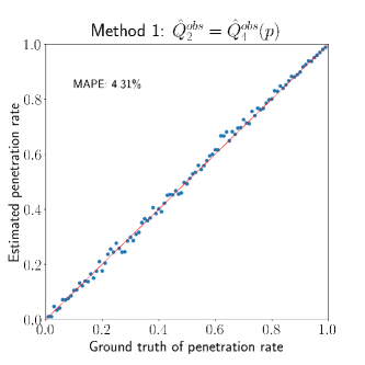
(a)

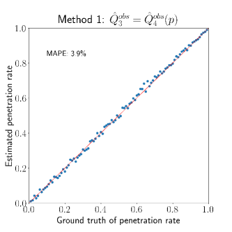
(b)

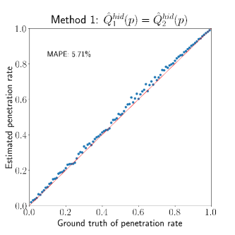
(c)

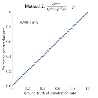
(d)

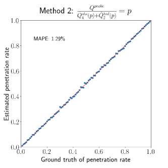
(e)

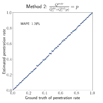
(f)

Figure 4: The results of penetration rate estimation using different methods

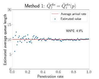
(a)

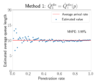
(b)

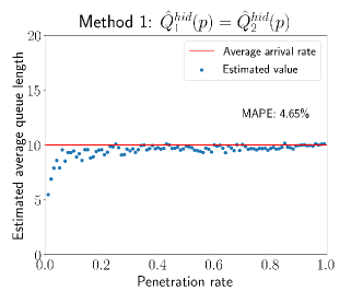
(c)

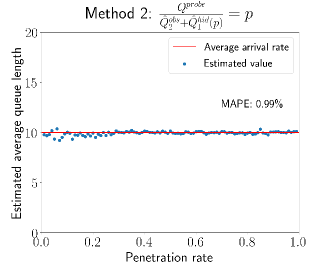
(d)

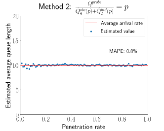
(e)

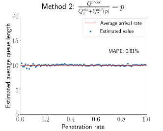
(f)

Figure 5: The results of queue length estimation using different methods

6.1.2 The effect of sample size

In order to demonstrate the impact of sample size on the estimation accuracy, the data of 100 cycles, 200 cycles, 500 cycles, and 1,000 cycles are used in four rounds of tests, respectively. The submethod $\frac{Q^{probe}}{\hat{Q}_{3}^{obs}(p)+\hat{Q}_{2}^{hid}(p)}=p$ is applied. The results in Figure 6 and Figure 7 show that better results can be obtained when the sample size is larger.

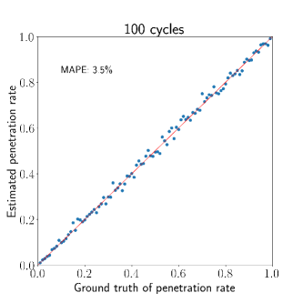
(a)

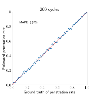
(b)

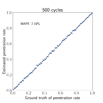
(c)

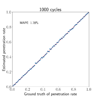
(d)

Figure 6: The results of penetration rate estimation with different sample sizes

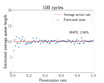
(a)

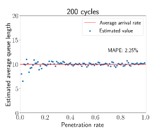
(b)

(c)

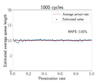
(d)

Figure 7: The results of queue length estimation with different sample sizes

6.1.3 The effect of the arrival rate during the red phase

To study the impact of the arrival rate on the estimation accuracy, the same submethod is applied to four different Poisson processes of which the average arrival rates are 3, 5, 10, and 15, respectively. In each test, 1,000 cycles of data are used. The results in Figure 8 and Figure 9 show that the larger the arrival rate is, the more accurate the estimation tends to be. The reason is that a higher arrival rate implies more observations of the probe vehicles, which could generally improve the estimation accuracy.

(a)

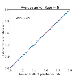
(b)

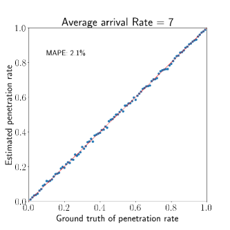
(c)

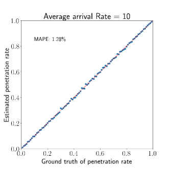
(d)

Figure 8: The results of penetration rate estimation with different arrival rates

(a)

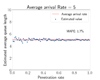
(b)

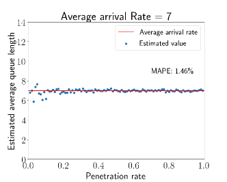
(c)

(d)

Figure 9: The results of queue length estimation with different arrival rates

6.1.4 The effect of overflow queues

In previous subsections, it is assumed that the queue in each cycle can be entirely discharged, that is, there are no overflow queues. In the real world, the number of vehicles arriving at an intersection in a cycle might exceed the number of vehicles the traffic signal can serve. To investigate the impact of the overflow queues on the estimation accuracy, the cases with overflow queues are also simulated. The simulation set-up of the overflow queues is similar to Comert and Cetin (2009). The average arrival rates in the green phase and in the red phase are set to 10. The maximum number of vehicles that can be served in each cycle is set to 22. The estimation results for penetration rates and queue lengths are shown in Figure 10. Since the simulation captures the effect of overflow queues, the average queue length is different from the average arrival rate in the red phase.

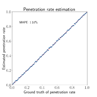
(a)

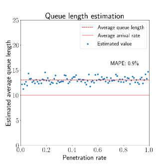
(b)

Figure 10: The estimation results of the cases with overflow queues: (a) penetration rate estimation, (b) queue length estimation

6.2 Real-world data

The proposed methods are also tested using real-world data. The focus of this test is on traffic volume estimation. Queue length estimation is not validated using real-world data because the ground truth of queue lengths is not available. The trajectory data are collected by Didi Chuxing from the vehicles offering its ride-hailing services in an area in Suzhou, Jiangsu Province, China, shown in Figure 11. The data of the 15 workdays from May 8, 2018, to May 28, 2018, are used for validation. The GPS trajectories of the Didi vehicles in the selected area are mapped onto the transportation network by a map matching algorithm (Newson and Krumm, 2009). For each movement and each one-hour time slot, the “snapshots” of the trajectory data are taken to extract the observed partial queues. Due to the accuracy of the trajectory data, the average space headway for the queueing vehicles could not be easily estimated. Therefore, its value is empirically set to 7.5 m/veh for the peak hours and 8.0 m/veh for the off-peak hours. For the movements with multiple lanes, since the accuracy of the trajectory data cannot reach the lane level, the stopping vehicles are randomly assigned to the different lanes. The random assignment process is repeated for 50 times to get an average estimate. Signal timing information from other data sources is not necessarily needed, as the trajectory data of the probe vehicles already contain some signal timing information. For instance, if the observed partial queue changes from $(0,0,1,0,0,0,1)$ to $(0,0,0,0,0,0,1)$, then it can be inferred that the latter queue is in the green phase because the first probe vehicle in the former queue has moved away. In general, the cycle length of the traffic signal ranges from 2 min to 3 min in the selected area. Therefore, for each movement and each time slot, the number of signal cycles of the evaluation period is in the range of 300 to 450.

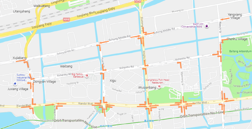
Figure 11: The studied movements in Suzhou

The methodology in this paper does not apply to the right-turn movements, as there might not be queues. Also, due to the accuracy of the data, it is almost impossible to deal with the lanes with mixed movements. The studied movements are represented by the arrows in Figure 11. In total, 22 through movements and 31 left-turn movements are studied.

Most of the signalized intersections in the selected area are covered by the camera-based automatic vehicle identification systems (AVIS) that can record the timestamps when vehicles go through the intersections. Nevertheless, not all the vehicles could be successfully identified by the cameras, and thus the vehicle counts given by the cameras are always smaller than the actual traffic volumes. Therefore, for each camera, its identification rate is estimated by the ratio of the number of identified Didi Vehicles and the total number of Didi vehicles passing the camera. Then, the real “ground truth” of the traffic volumes are projected by dividing the vehicle counts by the estimated identification rates. The estimated identification rates of three representative cameras during May 8, 2018, to May 15, 2018, are shown in Figure 12. The identification rates mostly vary from 80% to 100% during the day time, whereas the performance of the cameras becomes very unstable during the night time. Camera 1 outperforms camera 2 and camera 3 at night likely due to better lighting conditions. Considering the unstable accuracy during the night time, we only used the data collected from 8:00 to 19:00 for the validation.

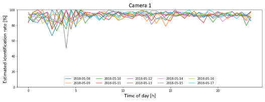
(a)

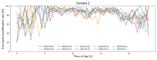
(b)

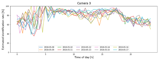
(c)

Figure 12: Accuracy of three typical cameras: (a) camera 1, (b) camera 2, (c) camera 3

6.2.1 Results

Figure 13 shows the results of traffic volume estimation for the studied through movements in six different time slots. The estimation results show that the applied method $\frac{Q^{probe}}{\hat{Q}_{3}^{obs}+\hat{Q}_{2}^{hid}(p)}=p$ can estimate traffic volume very accurately, which would be sufficient for most applications of mid-term or long-term signal control and performance measures. Figure 14 shows the results for the left-turn movements. The undermined performance further verifies the effect of the arrival rate on the estimation accuracy studied using the simulation data, since the traffic volumes of the left-turn movements are much smaller compared to the through movements.

Compared to the results of the simulation data, the estimation accuracy is undermined when the method is applied to the real-world data, due to the following reasons. First, although the map matching algorithm (Newson and Krumm, 2009) can mitigate the effect of GPS errors at the data preprocessing stage, the errors in the real-world trajectory data could still influence the estimation accuracy. Second, in the real world, for each movement and each one-hour time slot, the penetration rate and the queueing pattern might slightly vary during the studied 15 workdays. Third, the average space headway for the queueing vehicles is set empirically, which might introduce some biases into the results. If the data with better accuracy are available, the value of the average space headway should be estimated independently for each movement and each time slot.

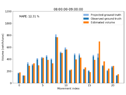
(a)

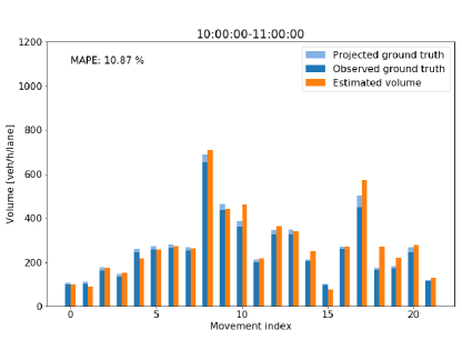
(b)

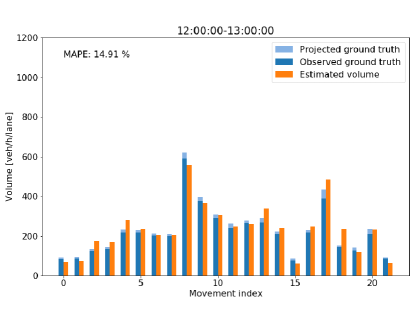
(c)

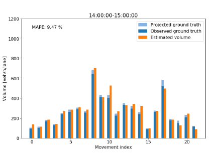
(d)

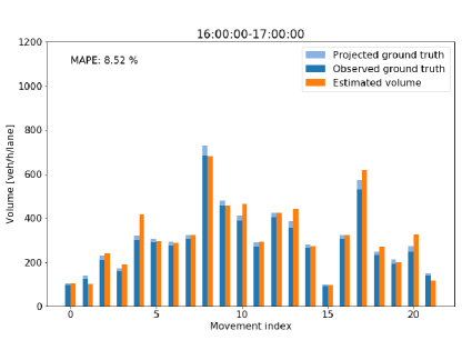
(e)

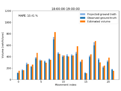
(f)

Figure 13: Traffic volume estimation results for the through movements in different TODs: (a) 08:00-09:00, (b) 10:00-11:00, (c) 12:00-13:00, (d) 14:00-15:00, (e) 16:00-17:00, (f) 18:00-19:00

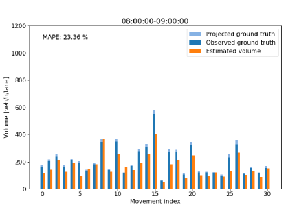
(a)

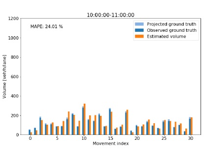
(b)

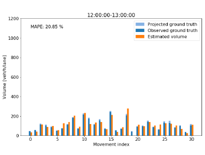
(c)

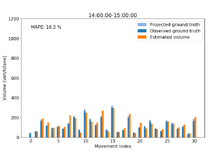
(d)

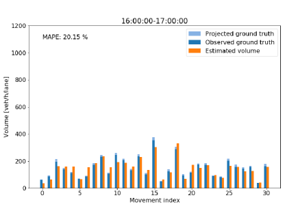
(e)

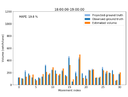
(f)

Figure 14: Traffic volume estimation results for the left-turn movements in different TODs: (a) 08:00-09:00, (b) 10:00-11:00, (c) 12:00-13:00, (d) 14:00-15:00, (e) 16:00-17:00, (f) 18:00-19:00

7 Conclusions

This paper proposes a general framework and a series of methods for the trajectory-based queue length and traffic volume estimation. For each specific movement and each specific time slot, the penetration rate of the probe vehicles is estimated by using the aggregated historical trajectory data of the probe vehicles. Once the penetration rate is estimated, it can be used to project the queue length and the traffic volume.

The proposed methods do not assume the type of vehicle arrival process or the queueing process. Therefore, the proposed methods are adaptable to both under-saturation and over-saturation cases. The proposed methods do not require high penetration rates and would be feasible for use in reality nowadays. The tests by both the simulation and the real-world data show good estimation accuracy, indicating that the proposed methods could be used for traffic signal control and performance measures at signalized intersections.

There are certain limitations in the current work that should be addressed in the future. For instance, the proposed methods in this paper take the stopping positions of the probe vehicles as the features to infer the penetration rate of the probe vehicles. However, there might not be queues forming at the non-signalized intersections or in the right-turn movements. Also, the queueing patterns in the shared left-through (right-through) lanes could be different from other left-turn (right-turn) lanes or through lanes. Therefore, when applying the proposed methods to these cases, additional care is required.

Appendix A

Definitions

For $k,n\in\mathbb{N}$ and $n\geq k$,

$$C_{n}^{k}=\frac{n!}{k!(n-k)!},$$ (A.1)

$$A_{n}^{k}=\frac{n!}{(n-k)!}.$$ (A.2)

Theorem 1

For conciseness, $Q_{i},N_{i},S_{i},T_{i},n_{i},s_{i},t_{i}$ are represented by $Q,N,S,T,n,s,t$, respectively.

$$\mathbb{E}(S\mid N=n,Q=l) =\frac{l+1}{n+1},$$ (A.3)

$$\mathbb{E}(Q\mid N=n)=\mathbb{E}(S\mid N=n)(n+1)-1,$$ (A.4)

where $n\geq 1$.

Proof:

$$\mathbb{E}(S\mid N=n,Q=l) =\sum_{j=1}^{l-n+1}P(S=j\mid N=n,Q=l)j$$ (A.5)

$$=\sum_{j=1}^{l-n+1}\frac{nC_{l-n}^{j-1}A_{j-1}^{j-1}A_{l-j}^{l-j}}{A_{l}^{l}}j$$ (A.6)

$$=\sum_{j=1}^{l-n+1}\frac{nA_{l-j}^{n-1}}{A_{l}^{n}}i$$ (A.7)

$$=\frac{n}{A_{l}^{n}}\sum_{j=1}^{l-n+1}A_{l-j}^{n-1}j$$ (A.8)

$$=\frac{n}{A_{l}^{n}}\sum_{k=0}^{l-n}A_{n+k-1}^{n-1}(l-n+1-k)$$ (A.9)

$$=\frac{n}{A_{l}^{n}}\sum_{k=0}^{l-n}A_{n+k-1}^{n-1}(l+1)-\frac{n}{A_{l}^{n}}\sum_{k=0}^{l-n}A_{n+k-1}^{n-1}(n+k)$$ (A.10)

$$=(l+1)\sum_{k=0}^{l-n}\frac{(n+k-1)!(l-n)!n!}{k!l!(n-1)!}-\frac{n}{A_{l}^{n}}\sum_{k=0}^{l-n}A_{n+k}^{n}$$ (A.11)

$$=\frac{l+1}{C_{l}^{n}}\sum_{k=0}^{l-n}C_{n+k-1}^{n-1}-\frac{n}{C_{l}^{n}}\sum_{k=0}^{l-n}C_{n+k}^{n}$$ (A.12)

$$=(l+1)\frac{C_{l}^{n}}{C_{l}^{n}}-n\frac{C_{l+1}^{n+1}}{C_{l}^{n}}$$ (A.13)

$$=(l+1)-n\frac{l+1}{n+1}$$ (A.14)

$$=\frac{l+1}{n+1}$$ (A.15)

Chu’s theorem (Merris, 2003) is applied when converting equation (A.12) to equation (A.13).

Then, based on the results above,

$$\mathbb{E}(S\mid N=n) =\sum_{j=1}^{L_{max}}P(S=j\mid N=n)j$$ (A.16)

$$=\sum_{j=1}^{L_{max}}\sum_{l=j+n-1}^{L_{max}}P(S=j\mid N=n,Q=l)P(Q=l\mid N=n)j$$ (A.17)

$$=\sum_{l=n}^{L_{max}}\sum_{j=1}^{l-n+1}P(S=j\mid N=n,Q=l)P(Q=l\mid N=n)j$$ (A.18)

$$=\sum_{l=n}^{L_{max}}P(Q=l\mid N=n)\sum_{j=1}^{l-n+1}P(S=j\mid N=n,Q=l)j$$ (A.19)

$$=\sum_{l=n}^{L_{max}}P(Q=l\mid N=n)\mathbb{E}(S\mid N=n,Q=l)$$ (A.20)

$$=\sum_{l=n}^{L_{max}}P(Q=l\mid N=n)\frac{l+1}{n+1}$$ (A.21)

$$=\frac{1}{n+1}\sum_{l=n}^{L_{max}}P(Q=l\mid N=n)(l+1)$$ (A.22)

$$=\frac{1}{n+1}\left(\mathbb{E}(Q\mid N=n)+1\right).$$ (A.23)

This is equivalent to

$$\mathbb{E}(Q\mid N=n)=\mathbb{E}(S\mid N=n)(n+1)-1.$$ (A.24)

Theorem 2

For conciseness, $Q_{i},N_{i},S_{i},T_{i},n_{i},s_{i},t_{i}$ are represented by $Q,N,S,T,n,s,t$, respectively.

$$\mathbb{E}(T\mid N=n,Q=l) =n\frac{l+1}{n+1},$$ (A.25)

$$\mathbb{E}(Q\mid N=n)=\mathbb{E}(T\mid N=n)\frac{n+1}{n}-1,$$ (A.26)

where $n\geq 1$.

Proof:

$$\mathbb{E}(T\mid N=n,Q=l) =\sum_{j=n}^{l}P(T=j\mid N=n,Q=l)j$$ (A.27)

$$=\sum_{j=n}^{l}\frac{nC_{l-n}^{l-j}A_{j-1}^{j-1}A_{l-j}^{l-j}}{A_{l}^{l}}j$$ (A.28)

$$=\sum_{j=n}^{l}\frac{nA_{j-1}^{n-1}}{A_{l}^{n}}j$$ (A.29)

$$=n\sum_{j=n}^{l}\frac{A_{j}^{n}}{A_{l}^{n}}$$ (A.30)

$$=n\sum_{j=n}^{l}\frac{C_{j}^{n}}{C_{l}^{n}}$$ (A.31)

$$=\frac{n}{C_{l}^{n}}\sum_{k=0}^{l-n}C_{n+k}^{n}$$ (A.32)

$$=\frac{nC_{l+1}^{n+1}}{C_{l}^{n}}$$ (A.33)

$$=n\frac{l+1}{n+1}$$ (A.34)

Then, based on the results above,

$$\mathbb{E}(T\mid N=n) =\sum_{j=n}^{L_{max}}P(T=j\mid N=n)j$$ (A.35)

$$=\sum_{j=n}^{L_{max}}\sum_{l=j}^{L_{max}}P(T=j\mid N=n,Q=l)P(Q=l\mid N=n)j$$ (A.36)

$$=\sum_{l=n}^{L_{max}}\sum_{j=n}^{l}P(T=j\mid N=n,Q=l)P(Q=l\mid N=n)j$$ (A.37)

$$=\sum_{l=n}^{L_{max}}P(Q=l\mid N=n)\sum_{j=n}^{l}P(T=j\mid N=n,Q=l)j$$ (A.38)

$$=\sum_{l=n}^{L_{max}}P(Q=l\mid N=n)\mathbb{E}(T\mid N=n,Q=l)$$ (A.39)

$$=\sum_{l=n}^{L_{max}}P(Q=l\mid N=n)n\frac{l+1}{n+1}$$ (A.40)

$$=\frac{n}{n+1}\sum_{l=n}^{L_{max}}P(Q=l\mid N=n)(l+1)$$ (A.41)

$$=\frac{n}{n+1}\left(\mathbb{E}(Q\mid N=n)+1\right).$$ (A.42)

This is equivalent to

$$\mathbb{E}(Q\mid N=n)=\mathbb{E}(T\mid N=n)\frac{n+1}{n}-1.$$ (A.43)

Theorem 3

For conciseness, $Q_{i},N_{i},S_{i},T_{i},n_{i},s_{i},t_{i}$ are represented by $Q,N,S,T,n,s,t$, respectively.

$$\mathbb{E}(Q\mid N\geq 1)=\mathbb{E}(S\mid N\geq 1)+\mathbb{E}(T\mid N\geq 1)-1$$ (A.44)

Proof:

First of all,

$$P(S=j\mid N\geq 1,Q=l)=p(1-p)^{j-1},\text{ if }1\leq j\leq l.$$ (A.45)

$$P(T=l-j+1\mid N\geq 1,Q=l) =p(1-p)^{l-(l-j+1)}$$ (A.46)

$$=p(1-p)^{j-1}$$ (A.47)

$$=P(S=j\mid N\geq 1,Q=l),\text{ if }1\leq j\leq l.$$ (A.48)

Then,

$$\mathbb{E}(S\mid N\geq 1) =\sum_{j=1}^{L_{max}}P(S=j\mid N\geq 1)j$$ (A.49)

$$=\sum_{j=1}^{L_{max}}\sum_{l=j}^{L_{max}}P(S=j\mid N\geq 1,Q=l)P(Q=l\mid N\geq 1)j$$ (A.50)

$$=\sum_{l=1}^{L_{max}}\sum_{j=1}^{l}P(S=j\mid N\geq 1,Q=l)P(Q=l\mid N\geq 1)j$$ (A.51)

$$=\sum_{l=1}^{L_{max}}\sum_{j=1}^{l}P(T=l-j+1\mid N\geq 1,Q=l)P(Q=l\mid N\geq 1)j$$ (A.52)

$$=\sum_{l=1}^{L_{max}}\sum_{k=1}^{l}P(T=k\mid N\geq 1,Q=l)P(Q=l\mid N\geq 1)(l-k+1)$$ (A.53)

$$\mathbb{E}(T\mid N\geq 1) =\sum_{k=1}^{L_{max}}P(T=k\mid N\geq 1)k$$ (A.54)

$$=\sum_{k=1}^{L_{max}}\sum_{l=k}^{L_{max}}P(T=k\mid N\geq 1,Q=l)P(Q=l\mid N\geq 1)k$$ (A.55)

$$=\sum_{l=1}^{L_{max}}\sum_{k=1}^{l}P(T=k\mid N\geq 1,Q=l)P(Q=l\mid N\geq 1)k$$ (A.56)

Therefore,

$$\mathbb{E}(S\mid N\geq 1)+\mathbb{E}(T\mid N\geq 1)-1 =\sum_{l=1}^{L_{max}}\sum_{k=1}^{l}P(T=k\mid N\geq 1,Q=l)P(Q=l\mid N\geq 1)(l-1)+1$$ (A.57)

$$=\sum_{l=1}^{L_{max}}P(Q=l\mid N\geq 1)(l-1)+1$$ (A.58)

$$=\sum_{l=1}^{L_{max}}P(Q=l\mid N\geq 1)l$$ (A.59)

$$=\mathbb{E}(Q\mid N\geq 1)$$ (A.60)

Alternatively, Theorem 3 can also be proved by combining Theorem 1 and Theorem 2.

References

- An et al. (2018) An, C., Wu, Y.-J., Xia, J., Huang, W., 2018. Real-time queue length estimation using event-based advance detector data. Journal of Intelligent Transportation Systems 22 (4), 277–290.
- Badillo et al. (2012) Badillo, B. E., Rakha, H., Rioux, T. W., Abrams, M., 2012. Queue length estimation using conventional vehicle detector and probe vehicle data. In: Intelligent Transportation Systems (ITSC), 2012 15th International IEEE Conference on. IEEE, pp. 1674–1681.
- Ban et al. (2011) Ban, X. J., Hao, P., Sun, Z., 2011. Real time queue length estimation for signalized intersections using travel times from mobile sensors. Transportation Research Part C: Emerging Technologies 19 (6), 1133–1156.
- Cai et al. (2014) Cai, Q., Wang, Z., Zheng, L., Wu, B., Wang, Y., 2014. Shock wave approach for estimating queue length at signalized intersections by fusing data from point and mobile sensors. Transportation Research Record: Journal of the Transportation Research Board 2422, 79–87.
- Cetin (2012) Cetin, M., 2012. Estimating queue dynamics at signalized intersections from probe vehicle data: Methodology based on kinematic wave model. Transportation Research Record: Journal of the Transportation Research Board 2315 (1), 164–172.
- Comert (2013a) Comert, G., 2013a. Effect of stop line detection in queue length estimation at traffic signals from probe vehicles data. European Journal of Operational Research 226 (1), 67–76.
- Comert (2013b) Comert, G., 2013b. Simple analytical models for estimating the queue lengths from probe vehicles at traffic signals. Transportation Research Part B: Methodological 55, 59–74.
- Comert (2016) Comert, G., 2016. Queue length estimation from probe vehicles at isolated intersections: Estimators for primary parameters. European Journal of Operational Research 252 (2), 502–521.
- Comert and Cetin (2009) Comert, G., Cetin, M., 2009. Queue length estimation from probe vehicle location and the impacts of sample size. European Journal of Operational Research 197 (1), 196–202.
- Comert and Cetin (2011) Comert, G., Cetin, M., 2011. Analytical evaluation of the error in queue length estimation at traffic signals from probe vehicle data. IEEE Transactions on Intelligent Transportation Systems 12 (2), 563–573.
- Guo et al. (2019) Guo, Q., Li, L., Ban, X. J., 2019. Urban traffic signal control with connected and automated vehicles: A survey. Transportation Research Part C: Emerging Technologies 101, 313–334.
- Hao and Ban (2015) Hao, P., Ban, X. J., 2015. Long queue estimation for signalized intersections using mobile data. Transportation Research Part B: Methodological 82, 54–73.
- Hao et al. (2015) Hao, P., Ban, X. J., Whon Yu, J., 2015. Kinematic equation-based vehicle queue location estimation method for signalized intersections using mobile sensor data. Journal of Intelligent Transportation Systems 19 (3), 256–272.
- Lee et al. (2015) Lee, S., Wong, S. C., Li, Y. C., 2015. Real-time estimation of lane-based queue lengths at isolated signalized junctions. Transportation Research Part C: Emerging Technologies 56, 1–17.
- Li et al. (2017) Li, F., Tang, K., Yao, J., Li, K., 2017. Real-time queue length estimation for signalized intersections using vehicle trajectory data. Transportation Research Record: Journal of the Transportation Research Board 2623, 49–59.
- Li et al. (2013) Li, J., Zhou, K., Shladover, S. E., Skabardonis, A., 2013. Estimating queue length under connected vehicle technology: Using probe vehicle, loop detector, fused data. Transportation Research Record: Journal of the Transportation Research Board 2366 (1), 17–22.
- Liu et al. (2009) Liu, H. X., Wu, X., Ma, W., Hu, H., 2009. Real-time queue length estimation for congested signalized intersections. Transportation Research Part C: Emerging Technologies 17 (4), 412–427.
- Merris (2003) Merris, R., 2003. Combinatorics. Vol. 67. John Wiley & Sons.
- Newson and Krumm (2009) Newson, P., Krumm, J., 2009. Hidden markov map matching through noise and sparseness. In: Proceedings of the 17th ACM SIGSPATIAL International Conference on Advances in Geographic Information Systems. ACM, pp. 336–343.
- Ramezani and Geroliminis (2015) Ramezani, M., Geroliminis, N., 2015. Queue profile estimation in congested urban networks with probe data. Computer-Aided Civil and Infrastructure Engineering 30 (6), 414–432.
- Rompis et al. (2018) Rompis, S. Y., Cetin, M., Habtemichael, F., 2018. Probe vehicle lane identification for queue length estimation at intersections. Journal of Intelligent Transportation Systems 22 (1), 10–25.
- Shahrbabaki et al. (2018) Shahrbabaki, M. R., Safavi, A. A., Papageorgiou, M., Papamichail, I., 2018. A data fusion approach for real-time traffic state estimation in urban signalized links. Transportation Research Part C: Emerging Technologies 92, 525–548.
- Wang et al. (2019) Wang, S., Huang, W., Lo, H. K., 2019. Traffic parameters estimation for signalized intersections based on combined shockwave analysis and bayesian network. Transportation Research Part C: Emerging Technologies 104, 22–37.
- Wang et al. (2017) Wang, Z., Cai, Q., Wu, B., Zheng, L., Wang, Y., 2017. Shockwave-based queue estimation approach for undersaturated and oversaturated signalized intersections using multi-source detection data. Journal of Intelligent Transportation Systems 21 (3), 167–178.
- Wong et al. (2019a) Wong, W., Shen, S., Zhao, Y., Liu, H. X., 2019a. On the estimation of connected vehicle penetration rate based on single-source connected vehicle data. Transportation Research Part B: Methodological 126, 169–191.
- Wong and Wong (2015) Wong, W., Wong, S., 2015. Systematic bias in transport model calibration arising from the variability of linear data projection. Transportation Research Part B: Methodological 75, 1–18.
- Wong and Wong (2019) Wong, W., Wong, S., 2019. Unbiased estimation methods of nonlinear transport models based on linearly projected data. Transportation Science 53 (3), 665–682.
- Wong and Wong (2016a) Wong, W., Wong, S. C., 2016a. Biased standard error estimations in transport model calibration due to heteroscedasticity arising from the variability of linear data projection. Transportation Research Part B: Methodological 88, 72–92.
- Wong and Wong (2016b) Wong, W., Wong, S. C., 2016b. Evaluation of the impact of traffic incidents using gps data. Proceedings of the Institution of Civil Engineers-Transport 169 (3), 148–162.
- Wong et al. (2019b) Wong, W., Wong, S. C., Liu, H. X., 2019b. Bootstrap standard error estimations of nonlinear transport models based on linearly projected data. Transportmetrica A: Transport Science 15 (2), 602–630.
- Zhan et al. (2017) Zhan, X., Zheng, Y., Yi, X., Ukkusuri, S. V., 2017. Citywide traffic volume estimation using trajectory data. IEEE Transactions on Knowledge & Data Engineering 2, 272–285.
- Zhao et al. (2019) Zhao, Y., Zheng, J., Wong, W., Wang, X., Meng, Y., Liu, H. X., 2019. Estimation of queue lengths, probe vehicle penetration rates, and traffic volumes at signalized intersections using probe vehicle trajectories. Transportation Research Record: Journal of the Transportation Research Board.
- Zheng and Liu (2017) Zheng, J., Liu, H. X., 2017. Estimating traffic volumes for signalized intersections using connected vehicle data. Transportation Research Part C: Emerging Technologies 79, 347–362.