Topological quantum matter with cold atoms

Abstract

This is an introductory review of the physics of topological quantum matter with cold atoms. Topological quantum phases, originally discovered and investigated in condensed matter physics, have recently been explored in a range of different systems, which produced both fascinating physics findings and exciting opportunities for applications. Among the physical systems that have been considered to realize and probe these intriguing phases, ultracold atoms become promising platforms due to their high flexibility and controllability. Quantum simulation of topological phases with cold atomic gases is a rapidly evolving field, and recent theoretical and experimental developments reveal that some toy models originally proposed in condensed matter physics have been realized with this artificial quantum system. The purpose of this article is to introduce these developments. The article begins with a tutorial review of topological invariants and the methods to control parameters in the Hamiltonians of neutral atoms. Next, topological quantum phases in optical lattices are introduced in some detail, especially several celebrated models, such as the Su-Schrieffer-Heeger model, the Hofstadter-Harper model, the Haldane model and the Kane-Mele model. The theoretical proposals and experimental implementations of these models are discussed. Notably, many of these models cannot be directly realized in conventional solid-state experiments. The newly developed methods for probing the intrinsic properties of the topological phases in cold atom systems are also reviewed. Finally, some topological phases with cold atoms in the continuum and in the presence of interactions are discussed, and an outlook on future work is given.

67.85.-d Ultracold gases, trapped gases; 03.75.Ss Degenerate Fermi gases; 73.43.Nq Quantum phase transitions; 71.10.Fd Lattices Fermi models; 03.75.Lm Tunneling Josephson effect, Boson-Einstein condensates in periodic potentials, solitons, vortices, and topological excitations; 03.65.Vf Phases: geometric, dynamic or topological

Contents

1. Introduction                                                                                              3

2. Topological invariants in momentum space                                                                     6
    2.1. Gauge fields in momentum space                                                              6
    2.2. Quantized Zak phase                                                                              7
    2.3. Chern numbers                                                                                     8
     2.4. Spin Chern number and $\mathbb{Z}_{2}$ topological invariants                                        9
    2.5. The Hopf invariant                                                                                  9

3. Engineering the Hamiltonian of atoms                                                                    10
    3.1. Laser cooling                                                                                      10
    3.2. Effective interactions                                                                             11
    3.3. Dipole potentials and optical lattices                                                             12
    3.4. Artificial magnetic fields and spin-orbit couplings                                                17
         3.4.1. Geometric gauge potentials                                                                        17
         3.4.2. Laser-assisted tunneling                                                                          21
         3.4.3. Periodically driven systems                                                                       23

4. Topological quantum matter in optical lattices                                                          26
    4.1. One-dimension                                                                                          27
         4.1.1. SSH model and Rice-Mele model                                                                     27
         4.1.2. Topological pumping                                                                               34
         4.1.3. 1D AIII class topological insulators                                                              37
         4.1.4. Creutz ladder model                                                                               39
         4.1.5. Aubry-Andre-Harper model                                                                          40
    4.2. Two-dimension                                                                                          42
         4.2.1. Graphene-like physics and Dirac fermions                                                          42
         4.2.2. Hofstadter model                                                                                  49
         4.2.3. Haldane model                                                                                     54
         4.2.4. Kane-Mele model                                                                                   58
    4.3. Three-dimension                                                                                        60
         4.3.1. 3D Dirac fermions                                                                                 60
         4.3.2. Weyl semimetals and Weyl fermions                                                                 61
         4.3.3. Topological nodal-line semimetals                                                                 65
         4.3.4. 3D $\mathbb{Z}_{2}$ topological insulators                                                                  67
         4.3.5. 3D Chiral topological insulators                                                                  69
         4.3.6. Hopf topological insulators                                                                       72
         4.3.7. Integer quantum Hall effect in 3D                                                                 75
    4.4. Higher and synthetic dimensions                                                                        78
    4.5. Higher-spin topological quasiparticles                                                                 82

5. Probing methods                                                                                         86
    5.1. Detection of Dirac points and topological transition                                                   86
    5.2. Interferometer in momentum space                                                                       87
    5.3. Hall drift of accelerated wave packets                                                                 90
    5.4. Streda formula and density profiles                                                                    92
    5.5. Tomography of Bloch states                                                                             93
    5.6. Spin polarization at high symmetry momenta                                                             96
    5.7. Topological pumping approach                                                                           98
    5.8. Detection of topological edge states                                                                   99

6. Topological quantum matter in continuous form                                                           99
    6.1. Jackiw-Rebbi model with topological solitons                                                           99
    6.2. Topological defects in Bose-Einstein condensates                                                      101
    6.3. Spin Hall effect in atomic gases                                                                      105

7. Topological quantum matter with interactions                                                           106
    7.1. Spin chains                                                                                           106
         7.1.1. Spin-1/2 chain                                                                                   106
         7.1.2. Spin-1 chain and Haldane phase                                                                   109
    7.2. Kitaev chain model                                                                                    111
    7.3. 1D Anyon-Hubbard model                                                                                116
    7.4. Bosonic quantum Hall states                                                                           118
         7.4.1. Single-component Bose-Hubbard model                                                              119
         7.4.2. Two-component Bose-Hubbard model                                                                 121
    7.5. Kitaev honeycomb model                                                                                122

8. Conclusion and outlook                                                                                 125
    8.1. Unconventional topological bands                                                                      125
    8.2. Other interacting topological phases                                                                  126
    8.3. Non-equilibrium dynamics and band topology                                                            127
    8.4. Topological states in open or dissipative systems                                                     128

Acknowledgements                                                                                                 129
Disclosure statement                                                                                                 129
Funding                                                                                                    129
Appendix A. Formulas of topological invariants                                                                   129

References                                                                                                 141

1 Introduction

Topology is an important mathematical discipline, starting its prosperity in the early part of the twentieth century. It is concerned with the properties of space that are preserved under continuous deformations, such as stretching, crumpling, and bending, but not tearing or gluing. Topological methods have recently played increasingly important roles in physics, and it is now difficult to think of an area of physics where topology does not apply. In early development in this field, Paul Dirac used topological concepts to show that there are magnetic monopole solutions to Maxwell’s equations [1], and Sir Roger Penrose also used topological methods to show that singularities are a generic feature of gravitational collapse [2]. However, it was not until the 1970’s that topology really came to prominence in physics, and that was thanks to its introduction into gauge theories and condensed matter physics.

What we now know as “topological quantum states” of condensed matter may go back to the Su-Schrieffer-Heeger model for conducting polymers with topological solitons in the 1970’s [3, 4, 5] and were encountered around 1980 [6], with the experimental discovery of the integer [7] and fractional [8] quantum Hall effects (QHE) in the two-dimensional (2D) electron systems, as well as the theoretical discovery of the entangled gapped spin-liquid states in quantum integer-spin chains [9]. Until then, phases of matter have been largely classified based on symmetries and symmetries breaking known as the Landau paradigm. The discovery of the “quantum topological matter” made it clear that the paradigm based on symmetries is insufficient, as the quantum Hall phases do not break any symmetry and would seem “trivial” from the symmetry standpoint.

A topological phase is an exotic form of matter characterized by non-local properties rather than local order parameters. An early milestone was the discovery by David Thouless and collaborators in 1982 of a remarkable formula [Thouless-Kohmoto-Nightingale-den Nijs (TKNN) formula] for QHE [10], which was soon recognized by Barry Simon as the first Chern invariant for the mathematically termed $U(1)$ fiber bundles in topology [11] with an essential connection to the geometric phase discovered by Michael Berry [12]. The identification of the TKNN formula as a topological invariant marked the beginning of the recognition that topology would play an important role in classifying quantum states. The TKNN result was originally obtained for the band structure of electrons in uniform magnetic fields. In 1988, F. D. M. Haldane realized that the necessary condition for a QHE was not a magnetic field, but broken time-reversal invariance [13]. He investigated a graphene-like tight-binding toy model (now called the Haldane model) with next-nearest-neighbor hopping and averaged zero magnetic field, constructing the first model for the QHE without Landau levels. The QHE without Landau levels is now known as the quantum anomalous Hall effect or Chern insulator, and is the first topological insulator discovered, although it is one with a broken time reversal symmetry (TRS). D. J. Thouless, J. M. Kostrlitz, and F. D. M. Haldane were awarded the 2016 Nobel Prize in physics “for theoretical discoveries of topological phase transitions and topological phases of matter”.

Another major development in this field is the discovery of topological insulators with TRS in 2-4 dimensions [14, 15]. S.-C. Zhang and J. Hu predicated a kind of four-dimensional QHE, which is characterized by the second Chern number [16]. It is the first topological insulator with TRS predicted and only recently was experimentally realized with ultracold atoms [17]. C. Kane and E. Mele [18, 19] theoretically combined two conjugate copies of the Haldane model, one for spin-up electrons for which the valence band has Chern number $\pm 1$ and one for spin-down electrons where the valence band has the opposite Chern number $\mp 1$. Since the total Chern number of the band vanishes, there is no QHE. However, they discovered that so long as the TRS is unbroken, the system has a previously unexpected $\mathbb{Z}_{2}$ topological invariant related to Kramers degeneracy. Independently, B. A. Bernevig, T. L. Hughes, and S.-C. Zhang [20] predicted the quantum spin Hall effect [21] in quantum well structures of HgCdTe, which is known as a state of 2D topological insulators, paving the way to its experimental discovery [22]. The 3D generalization of this $\mathbb{Z}_{2}$ invariant was independently and simultaneously predicted in 2007 by three groups [6], which led to the experimental discovery of the 3D time reversal invariant topological insulators. The discovery of topological insulators signaled the start of a wider search for topological phases of matter, and this continues to be fertile ground. Since topological quantum numbers are fairly insensitive to local imperfections and perturbations, topological protection offers fascinating possibilities for applications in quantum technology.

Besides topological insulators, topological phases are generalized to topological (semi)metals, such as Weyl and Dirac semimetals in 3D solids [23, 24], and new topological materials are being discovered and developed at an impressive rate, the possibilities for creating and probing exotic topological phases would be greatly enhanced if these phases could be realized in systems that are easily tuned. Ultracold atoms with their flexibility could provide such a platform. In particular, some idealized model Hamiltonians for topological quantum matter, which are unrealistic in other quantum systems, can be realized with ultracold atoms in optical lattices (OLs). Below, we briefly summarize the toolbox that has been developed to create and probe topological quantum matter with cold atoms.

i) The lattice structure of a single-particle energy band in a solid is fundamental for some topological quantum phases. For instance, both the topological insulators proposed by Handane and Kane and Mele exist in a honeycomb lattice, while spin liquid states favor a Kagome lattice. Ultracold atoms can be trapped in the potential minima formed by the laser beams. By changing the angles, wavelengths and polizations of the laser beams, one can create different lattice geometries. OLs with various geometric structures, such as square/cubic, triangular, honeycomb, and Kagome lattice, and superlattice structures, have been experimentally realized (see the review on engineering novel OLs [25]). In addition, OLs provide convenient ways to control various factors in cold atoms such as the strength of interatomic interactions, the band structures, the spin composition, and the levels of disorder more easily than in real crystals.

ii) A necessary condition for the QHE or topological insulators with broken TRS is a magnetic field (flux). Although atomic gases are neutral particles, artificial gauge fields can be realized for them [26, 27]. Therefore, one can use atomic gases to simulate charged quantum particles, such as electrons in external electromagnetic fields. Artificial magnetic fields for atomic gases have been implemented through several ways: rotating an isotropic 2D harmonic trap, generating a space-dependent geometric phase by dressing the atom-light interaction, and suitably shaking an OL. Importantly, the methods based on the atom-light interaction and shaking lattices are well-suited for implementing an artificial gauge field in an OL. Artificial gauge fields, combined with OLs, lead to the realization of several celebrated toy models proposed but unrealistic in condensed matter physics. For instance, the Haldane model [28] and the Hofstadter model [29, 30] have been directly realized for the first time with ultracold gases.

iii) Spin-orbit coupling (SOC) is a basic ingredient for a $\mathbb{Z}_{2}$ topological insulator with TRS. It can also be realized by a non-Abelian geometric phase due to the atom-laser interaction. To simulate an SOC of spin-1/2 particles, one can use a configuration where two atomic dressed states form a degenerate manifold at every point in the laser field. When an atom prepared in a state in the manifold slowly moves along a closed trajectory, a non-Abelian geometric phase is accumulated in the wave function, and an SOC is generated if the non-Abelian geometric phase is space dependent. Recently, one-dimensional (1D) and 2D SOCs for bosonic and fermionic atoms have been experimentally created in the continuum or OLs [31, 32, 33, 34, 35, 36], which are the first step towards the simulation of a topological insulator with TRS.

iv) The concept of synthetic dimensions offers an additional advantage for the experimental exploration of topological states in cold gases. One kind of synthetic dimension consists of interpreting a set of addressable internal states of an atom, e.g. Zeeman sublevels of a hyperfine state as fictitious lattice sites; this defines an extra spatial dimension coined synthetic dimension. Therefore, driving transitions between different internal states corresponds to inducing hopping processes along the synthetic dimension. In turn, loading atoms into a real N-dimensional spatial OL potentially allows one to simulate systems of $N+1$ spatial dimensions. Synthetic dimensions were recently realized in 1D OLs for investigating the chiral edge states in the 2D QHE [37, 38, 39]. Notably a dynamical version of the 4D QHE [16, 40, 41] has been experimentally achieved with cold atoms in a 2D optical superlattice with two synthetic dimensions [17].

v) Besides the possibility of engineering single particle Hamiltonians, there are several methods to flexibly tune complex many-body interactions in cold atoms. Strong correlation plays important roles for some typical topological quantum matter, such as fractional quantum Hall states and spin liquids. More recently, there has been intense interest in the possibility of realizing fractional quantum Hall states in lattice systems: the fractional Chern insulators. The tunability of atomic on-site interactions [42] or long-range dipole-dipole interactions in ultracold dipolar gases [43, 44] opens up the possibility of realizing various new topological states with strong correlations, including fractional anyonic statistics, an unambiguous signature of topological phases.

vi) Compared with condensed-matter systems, ultracold atoms allow detailed studies of the relation between dynamics and topology as the timescales are experimentally easier to access. For example, time-dependent OLs constitute a powerful tool for engineering atomic gases with topological properties. Recently, the identification of non-equilibrium signatures of topology in the dynamics of such systems has been reported by using time- and momentum-resolved full state tomography for spin-polarized fermionic atoms in driven OLs [45, 46, 47]. These results pave the way for a deeper understanding of the connection between topological phases and non-equilibrium dynamics.

vii) Another remarkable advantage for studying topological phases with cold atoms is that the topological invariants can be directly detected in this system. For example, the Chern number has been directly detected by measuring the quantized center-of-mass response [48]. It can also be observed through the Berry-curvature-reconstruction scheme [45, 46] or by measuring the spin polarization of an atomic cloud at highly-symmetric points of the Brillouin zone (BZ) [36]. Furthermore, nontrivial edge states can be visualized in real space since the high-resolution addressing techniques offer the possibility of directly loading atoms into the edge states and cold atoms can be visualized by imaging the atomic cloud in-situ. Momentum distributions and band populations can also be obtained through time-of-flight imaging and band-mapping, respectively.

In this review, we take a closer look at the merger of two fields: topological quantum matter as discussed in condensed matter physics and ultracold atoms. Both are active fields of research with a large amount of literature. For readers interested in more specialized reviews of quantum simulation with ultracold atoms, we recommend review articles [49, 50, 51, 26, 52, 53, 54, 27, 55, 56, 57, 58, 59]. For readers interested in more dedicated reviews on topological phases in condensed matter, we recommend Refs. [14, 15, 23, 60, 61, 24]. The aim of this review is to satisfy the needs of both newcomers and experts in this interdisciplinary field. To cater to the needs of newcomers, we devote Sec. 2 to a tutorial-style introduction to topological invariants commonly used in condensed matter physics, and the more general introductions are put in the Appendix A. In Sec. 3, we describe how the Hamiltonians can be fully engineered in cold atom systems. A reader new to condensed matter physics or ultracold atomic physics would find these two sections beneficial. In Sec. 4, our emphasis is on recent theoretical and experimental developments on how to realize various topological states (models) or phenomena in different OL systems. In Sec. 5, we introduce the developed methods for probing topological invariants and other intrinsic properties of the topological phases in cold atom systems. In Sec. 6 and Sec. 7, we move beyond single-particle physics of Bloch bands in lattice systems to describe some quantum matter in the continuum and interacting many-body phases that have topologically nontrivial properties. Finally, an outlook on future work and a brief conclusion are given.

2 Topological invariants in momentum space

The purpose of this section is to briefly introduce various topological invariants referenced in the following sections. The more general introduction of topological invariants with the derivations of many formulas in this section are put in the Appendix A.

2.1 Gauge fields in momentum space

We denote the momentum-space Hamiltonian of an insulator as $\mathcal{H}(\mathbf{k})$ with $\mathbf{k}$ in the first Brillouin zone (BZ), and assume finite number of bands, namely $\mathcal{H}(\mathbf{k})$ is a $(M+N)$-dimensional matrix at each $\mathbf{k}$, where $M$ and $N$ are numbers of conduction and valence bands, respectively. At each $\mathbf{k}$, $\mathcal{H}(\mathbf{k})$ can be diagonalized and the conduction and valence eigenpairs are $(E_{+,a},\leavevmode\nobreak\ |+,\mathbf{k},a\rangle)$ and $(E_{-,b},\leavevmode\nobreak\ |-,\mathbf{k},b\rangle)$, respectively, with $a=1,\cdots,M$ and $b=1,\cdots,N$. At each $\mathbf{k}$, valence states $|-,\mathbf{k},b\rangle$ span an $N$ dimensional vector space and these vector space spread smoothly over the whole BZ. We can define the Berry connection (gauge potential) as

$$\mathcal{A}_{b,b^{\prime}}^{\mu}(\mathbf{k})=\langle-,\mathbf{k},b|\frac{\partial}{\partial k_{\mu}}|-,\mathbf{k},b^{\prime}\rangle$$ (1)

with $\mu=1,2,\cdots,d$ labeling momentum coordinates. Accordingly, the Berry curvature (gauge field strength) is given by

$$\mathcal{F}^{\mu\nu}=\partial^{\mu}\mathcal{A}^{\nu}-\partial^{\nu}\mathcal{A}^{\mu}+[\mathcal{A}^{\mu},\mathcal{A}^{\nu}].$$ (2)

To have a basic idea of the Berry connection and curvature in momentum space, we take a general two-band model as an example. The Hamiltonian reads

$$\mathcal{H}_{2b}(\mathbf{k})=\mathbf{d}(\mathbf{k})\cdot\sigma,$$ (3)

where $\sigma_{i}$ with $i=1,2,3$ are the Pauli matrices. Strictly speaking, the term $\epsilon(\mathbf{k})\mathrm{1}_{2}$ should also be added into Eq. (3). But it is ignored here because it is irrelevant to the topology of the band structure, noticing that it only shifts the energy spectrum and does not affect eigenstates. As the spectrum is given by $E_{\pm}(\mathbf{k})=\pm|\mathbf{d}(\mathbf{k})|$, for insulator $|\mathbf{d}(\mathbf{k})|$ is not equal to zero for all $\mathbf{k}$. The valence eigenstates can be represented by $|-,\mathbf{k}\rangle=e^{-i\sigma_{3}\phi(\mathbf{k})/2}e^{-i\sigma_{2}\theta(\mathbf{k})/2}|\downarrow\rangle$, where $\theta(\mathbf{k})$ and $\phi(\mathbf{k})$ are the standard spherical coordinates of $\hat{\mathbf{d}}(\mathbf{k})\equiv\mathbf{d}(\mathbf{k})/|\mathbf{d}(\mathbf{k})|$, and $|\downarrow\rangle$ is the negative eigenstate of $\sigma_{3}$. The Berry connection can be straightforwardly derived as

$$\mathcal{A}^{\mu}(\mathbf{k})=\frac{i}{2}\text{cos}\theta(\mathbf{k})\,\partial^{\mu}\phi(\mathbf{k}).$$ (4)

Under the $U(1)$ gauge transformation $|-,\mathbf{k}\rangle\rightarrow e^{i\varphi(\mathbf{k})}|-,\mathbf{k}\rangle$, the Berry connection $\mathcal{A}^{\mu}(\mathbf{k})$ is transformed to be $\mathcal{A}^{\mu}(\mathbf{k})+i\partial_{k_{\mu}}\varphi(\mathbf{k})$. But the Berry curvature is invariant under gauge transformations, and is given from Eq. (2) by $\mathcal{F}^{\mu\nu}(\mathbf{k})=-\frac{i}{2}\text{sin}\theta(\mathbf{k})[\partial^{\mu}\theta(\mathbf{k})\partial^{\nu}\phi(\mathbf{k})-\partial^{\nu}\theta(\mathbf{k})\partial^{\mu}\phi(\mathbf{k})]$, which can be recast in terms of $\hat{\mathbf{d}}(\mathbf{k})$ as

$$\mathcal{F}^{\mu\nu}(\mathbf{k})=\frac{1}{2i}\hat{\mathbf{d}}\cdot(\partial^{\mu}\hat{\mathbf{d}}\times\partial^{\nu}\hat{\mathbf{d}}).$$ (5)

2.2 Quantized Zak phase

The simplest example of topological invariant in momentum space is the so-called quantized Zak phase. The Zak phase is a Berry’s phase picked up by a particle moving across a 1D BZ [62]. For a given Bloch wave $\psi_{k}(x)$ with quasimomentum $k$, the Zak phase can be conveniently expressed through the cell-periodic Bloch function $u_{k}(x)=e^{-ikx}\psi_{k}(x)$:

$$\gamma=i\int_{-G/2}^{G/2}\mathcal{A}_{k}dk,$$ (6)

where the gauge potential in Eq. (1) is given by $\mathcal{A}_{k}=\langle u_{k}|\partial_{k}|u_{k}\rangle$ and $G=2\pi/a$ is the reciprocal lattice vector and $a$ is the lattice period. As $i\partial_{k}$ in Eq. (6) is the position operator, physically $\gamma a/(2\pi)$ is just the center of the Wannier function corresponding to $u_{k}(x)$. Accordingly, it is noticed that the Zak phase $\gamma$, Eq. (6), is well defined module $2\pi$, because a shift of the lattice origin by $d$, which corresponds to $u_{k}(x)\rightarrow e^{ikd}u_{k}(x)$, changes Eq. (6) by $2\pi d/a$. So the Zak phase $\gamma$ can be any real number mod $2\pi$, and therefore is not a topological invariant. However, certain symmetries can quantize it into integers in units of $\pi$. The quantization of Eq. (6) was first discussed in 1D band theory by Zak taking into account the inversion symmetry [62]. In order to preserve the inversion symmetry, the wanner-function center has to be either concentrated at lattice sites or at the midpoints of lattice sites.

A paradigmatic 1D model with the topological invariant being the Zak phase is provided by the Su-Schrieffer-Heeger model of polyacetylene [3], which exhibits two topologically distinct phases. A unit cell in this model has two sites with sublattice symmetry, which quantizes the Zak phase. Accordingly the cell-periodic wave function $u_{k}$ can be viewed as a two-component spinor $u_{k}=(\alpha_{k},\beta_{k})$, and the Zak phase, Eq. (6), in units of $\pi$ takes an simple form $\nu_{Z}=(i/\pi)\int_{-G/2}^{G/2}(\alpha_{k}^{*}\partial_{k}\alpha_{k}+\beta_{k}^{*}\partial_{k}\beta_{k})dk$.

2.3 Chern numbers

The second example of the topological invariants in momentum space is the famous Chern number, which can be formulated for any even-dimensional spaces. For $2n$ dimensions, the corresponding Chern number is called the $n$th Chern number, and the corresponding integrand is called the $n$th Chern character. We first introduce the first Chern number (conventionally called Chern number), which appears in 2D momentum space $\mathbf{k}=(k_{x},k_{y})$. The BZ forms a torus $\mathbb{T}^{2}$ and the Chern number for a $2$D insulator is given as

$${C}=\frac{i}{2\pi}\int_{\mathbb{T}^{2}}d^{2}k\leavevmode\nobreak\ \mathrm{tr}\mathcal{F}^{xy}.$$ (7)

Noticing that the trace over the commutator in Eq. (2) vanishes, we find that the Chern number essentially comes from the Abelian connection $a^{\mu}=\mathrm{tr}\mathcal{A}^{\mu}$, which is just the sum of the Abelian Berry connection of all valence bands, namely, that $a^{j}=\sum_{\alpha}\langle\mathbf{k},\alpha|\partial/\partial k_{j}|\mathbf{k},\alpha\rangle$ with $\alpha$ labeling the valence bands. Accordingly the Chern number of Eq. (7) can be rewritten in terms of the Abelian connection as

$${C}=\frac{i}{2\pi}\int\int_{BZ}f^{xy}\mathbf{(k)}dk_{x}dk_{y},\ \ \ f^{xy}\mathbf{(k)}=\frac{\partial a^{y}\mathbf{(k)}}{\partial k_{x}}-\frac{\partial a^{x}\mathbf{(k)}}{\partial k_{y}},$$ (8)

The Chern number of Eq. (7) is also called the Thouless-Kohmoto-Nightingale-den Nijs (TKNN) invariant, which was shown to be the transverse conductance in units of $e^{2}/h$ using the Kubo formula, and therefore is the topological invariant to characterize the integer quantum Hall effect [10]. A nonvanishing transverse conductance requires the TRS breaking, which is consistent with Eq. (7), since $i\mathcal{F}$ is odd under TRS. For the two-band model of Eq. (3), the Chern number can be expressed explicitly by

$$C=\frac{1}{4\pi}\int\int_{BZ}\leavevmode\nobreak\ \hat{\mathbf{d}}\cdot(\partial_{k_{x}}\hat{\mathbf{d}}\times\partial_{k_{y}}\hat{\mathbf{d}})dk_{x}dk_{y},$$ (9)

which can be derived by directly substituting Eq. (5) into Eq. (8).

If $n=2$, the second Chern number for a $4$D insulator is given by

$${C}_{2}=-\frac{1}{32\pi^{2}}\int_{\mathbb{T}^{4}}d^{4}k\leavevmode\nobreak\ \epsilon_{\mu\nu\lambda\sigma}\mathrm{tr}\mathcal{F}^{\mu\nu}\mathcal{F}^{\lambda\sigma}.$$ (10)

For more than one valence bands, the second Chern number, Eq. (10), cannot be expressed in terms of the Abelian Berry connection $a^{\mu}(\mathbf{k})$, which is in contrast to the first Chern number, and therefore is essentially non-Abelian. It was predicted that the second Chern number ${C}_{2}$ can be used to characterize a quantum Hall effect in 4D space [16], which was realized in a recent experiment with ultracold atoms loaded in an optical lattice with synthetic dimensions [17]. Furthermore, in contrast to that all systems with TRS have vanishing first Chern number, the second Chern number of Eq. (10) can preserve TRS, namely, that there exist nontrivial time-reversal-invariant $4$D Chern insulators. In addition, the meaning of the second Chern number for electromagnetic response can be found in Refs. [63, 64].

Let us consider isolated gap-closing points in a $(2n+1)$D BZ, where the Berry connection is not well-defined. Although the Berry connection is singular at any gap-closing point, a $(2n)$D sphere $\mathbb{S}^{2n}$ can be chosen to enclose it, restricted on which the spectrum is gapped with the well-defined Berry connection. Accordingly the Chern number can be calculated on the $\mathbb{S}^{2n}$, and is referred to as the monopole charge of the singular point. For monopoles in $3$D space, the monopole charge can be calculated by the Abelian Berry connection $a^{\mu}=\mathrm{tr}\mathcal{A}^{\mu}$, and therefore are termed as Abelian monopoles. For instance the Weyl points described by the Hamiltonian $\mathcal{H}_{W}(\mathbf{k})=\pm\mathbf{k}\cdot\sigma$ can be interpreted as unit Abelian monopoles in momentum space for the respective Abelian gauge field of valence band restricted on $\mathbb{S}^{2}$ surrounding the origin. The monopole charges defined in higher dimensions are introduced in the Appendix.

2.4 Spin Chern number and $\mathbb{Z}_{2}$ topological invariants

We further consider particles with spin-1/2 (or pseudo-spin-1/2) in 2D momentum space. If the $U(1)$ spin-rotation symmetry to any specific direction (denoted as $z$-direction here) is preserved, the corresponding spin polarization $s=\uparrow,\downarrow$ is a good quantum number, and therefore the notation $|\mathbf{k},\alpha\rangle$ of valence bands used above should be refined as $|\mathbf{k},\alpha,s\rangle$. Then each spin $s$ can be individually assigned a Chern number $C_{s}$ as that of Eq. (8), which is the sum of the Chern numbers of all valence bands with the corresponding spin $s$ and naturally integer valued. As a topological insulator it is now characterized by two topological indices, the usual Chern number $C$ and the spin Chern number $C_{s}$ [65], respectively given by

$$C=C_{\uparrow}+C_{\downarrow},\ \ \ \ C_{s}=(C_{\uparrow}-C_{\downarrow})/2.$$ (11)

Provided TRS is preserved (thus $C=0$) as well as the $U(1)$ spin-rotation symmetry, the spin Chern number $C_{s}$ is also integer valued. In this case $C_{s}$ can be used to characterized the quantum spin Hall effect [65].

Notably, the $U(1)$ spin-rotation symmetry can usually be broken by generic spin-orbital couplings and therefore is not a good symmetry, but TRS is still preserved in the absence of magnetic field. In the general situation with only TRS, the spin Chern number $C_{s}$ is no longer well-defined and should be replaced by a $\mathbb{Z}_{2}$ topological invariant for characterizing the 2D topological insulators with TRS [19, 21, 20], which was first proposed by Kane and Mele in Ref. [18]. The $\mathbb{Z}_{2}$ topological invariants proposed there can be generalized to characterize 3D time-reversal-invariant topological insulators. These $\mathbb{Z}_{2}$ topological invariants are briefly introduced in the Appendix A.

2.5 The Hopf invariant

There is a kind of topological insulator restricted in both two bands and three dimensions. For a two-band insulator, the Hamiltonian (3) at each $\mathbf{k}$ can be topologically regarded as a point $\hat{d}(\mathbf{k})$ on a unit sphere $\mathbb{S}^{2}$, and thereby it gives a mapping from the $3$D BZ to $\mathbb{S}^{2}$. Because of the homotopy group $\pi_{3}(\mathbb{S}^{2})\cong\mathbb{Z}$, there exist (strong) $3$D two-band topological insulators with $\mathbb{Z}$ classification, which is termed the Hopf insulators [66]. The corresponding topological invariant is called the Hopf invariant [67, 66], and is given by

$$\nu_{H}=-\frac{1}{4\pi^{2}}\int_{\mathbb{T}^{3}}d^{3}k\leavevmode\nobreak\ \epsilon_{\mu\nu\lambda}\mathcal{A}^{\mu}\partial^{\nu}\mathcal{A}^{\lambda},$$ (12)

where $\mathcal{A}^{\mu}=\langle-,\mathbf{k}|\partial_{k_{\mu}}|-,\mathbf{k}\rangle$ is the Berry connection of the valence band defined in Eq. (1).

3 Engineering the Hamiltonian of atoms

For particles of mass $m$ and index $i$, charge $q$ and magnetic moment $\mathbf{\mu}_{B}$, in an electromagnetic field described by the vector potential $\mathbf{A}=(A_{x},A_{y},A_{z})$ and scalar potential $V(\mathbf{r})$, the Hamiltonian is given by

$$H=\sum_{i}\left[\frac{1}{2m}(\mathbf{p}_{i}-q\mathbf{A})^{2}+V(\mathbf{r}_{i})-\mathbf{\mu}_{B}\cdot\mathbf{B}(\mathbf{r}_{i})\right]+U_{\text{int}},$$ (13)

where $\mathbf{p}_{i}=-i\hbar\nabla_{i}$ is the momentum operator, $\mathbf{B}$ is the magnetic field, and $U_{\text{int}}$ is the Hamiltonian caused by the interaction between particles. One of the great advantages of ultracold atomic systems is that, all terms in the Hamiltonian (13) are tunable in experiments, and thus many exotic quantum phases, including various topological phases addressed latter in this review, can be realized. In this section, we first briefly review the methods to modify the mean kinetic energy $\langle p_{i}^{2}\rangle/2m$ related to the temperature and the interaction $U_{\text{int}}$, and then address more detailed the approaches to engineer the so-called artificial gauge fields for neutral atoms (the vector potential $\mathbf{A}$, the scalar potential $V(\mathbf{r}_{i})$, and the effective Zeeman field $\mathbf{B}(\mathbf{r}_{i})$), which are fundamentally important in creating various exotic topological phases.

3.1 Laser cooling

The mean kinetic energy of the atoms $\langle p_{i}^{2}\rangle/2m$ is mainly determined by the temperature of the atomic cloud and can be controlled by laser cooling, which refers to a number of techniques in which atomic samples are cooled down to near absolute zero. Laser cooling techniques rely on the fact that when an atom absorbs and re-emits a photon its momentum changes. For an ensemble of particles, their temperature is proportional to the variance in their velocities. That is, more homogeneous velocities among particles corresponds to a lower temperature. Laser cooling techniques combine atomic spectroscopy with the mechanical effect of light to compress the velocity distribution of an ensemble of particles, thereby cooling the particles. A Nobel prize was awarded to three physicists, S. Chu, C. N. Cohen-Tannoudji, and W. D. Phillips, for their achievements of laser cooling of atoms in 1997.

The first proposal of laser cooling by Hänsch and Schawlow in 1974 [68] was based upon Doppler cooling in a two-level atom. It was suggested that the Doppler effect due to the thermal motion of atoms could be exploited to make them absorb laser light at a different rate depending on whether they moved away from or toward the laser. Consider an atom irradiated by counterpropagating laser beams that are tuned to the low frequency side of atomic resonance. The beam counterpropagating with the atom will be Doppler shifted towards resonance, thus increasing the probability of photon absorption. The beam co-propagating with the atom will be frequency-shifted away from resonance, so there will be a net absorption of photons opposing the motion of the atom. The net momentum kick felt by the atom could then be used to slow itself down. By surrounding the atom with three pairs of counter-propagating beams along the $x$, $y$ and $z$ axes, one can generate a drag force opposing the velocity of the atom. The term ”optical molasses” was coined to describe this situation.

When this simple principle was finally applied in the early 1980s, it immediately led to low temperatures only a few hundreds of micro-Kelvins above absolute zero. As an example, the mean velocity of a ⁸⁷Rb atomic gas in temperature of $100$ mK is about $0.17$ m/s, which is much slower than the velocity of several hundred meters per second at room temperature. Ultracold atoms also turned out to be an ideal raw material for the realization of magnetic traps for neutral atoms. Held in place by magnetic dipole forces, such atomic gases can then be evaporatively cooled by successively lowering the trap depth, thus letting the most energetic atoms escape and allowing the remaining ones to rethermalize. In this way, the fundamental limitations of laser cooling due to photon scattering can be overcome and the temperature as low as a few nano-Kelvins can be reached. The mean velocity of a ⁸⁷Rb atomic gas in temperature of $1$ nK is about $5.3\times 10^{-4}$ m/s.

3.2 Effective interactions

The term $U_{\text{int}}$ in Eq. (13) is induced by interatomic interactions and can be manipulated with a powerful method called the Feshbach resonance (for a review, see Ref. [42]). The fundamental result for the atom-atom scattering is that under appropriate conditions, the effective interaction potential $U_{\text{int}}(\mathbf{r}=\mathbf{r}_{i}-\mathbf{r}_{j})$ of two atoms (particle indices $i$ and $j$) of reduced mass $m_{r}$ can be replaced by a delta function of strength $2\pi\hbar^{2}a_{s}/m_{r}$, where $a_{s}$ is the low-energy $s$-wave scattering length. As for two similar particles with mass $m$, the commonly quoted form of the effective interaction is

$$U_{\text{int}}(\mathbf{r})=\frac{4\pi a_{s}\hbar^{2}}{m}\delta(\mathbf{r}).$$ (14)

Alternative, it can be understood in the following way: the mean interaction energy of the many-body system is given by the expression

$$\langle E_{\text{int}}\rangle=\frac{1}{2}\frac{4\pi a_{s}\hbar^{2}}{m}\sum_{ij}|\Psi(r_{ij}\rightarrow 0)|^{2},$$ (15)

where $\Psi$ is the many-body wave function and the notation $r_{ij}\rightarrow 0$ means that the separation $r_{ij}$ of the two atoms, while large compared to $a_{s}$, is small compared to any other characteristic length (e.g., thermal de Broglie wavelength, interparticle spacing, etc). The conditions necessary for the validity of Eq. (15) in the time-independent case are the following: First, the orbital angular momentum $l\neq 0$ scattering must be negligible. Second, the existence of the limit $r_{ij}\rightarrow 0$ implies the condition $k_{c}a_{s}\ll 1$, where $k_{c}$ is the characteristic wave-vector scale of the many-body wave function $\Psi$ (for a very general argument, see Ref. [69]).

The scattering length $a_{s}$ can be manipulated by a Feshbach resonance [42]. It occurs when the bound molecular state in the closed channel energetically approaches the scattering state in the open channel. Then even weak coupling can lead to strong mixing between the two channels. The energy difference can be controlled via a magnetic field when the corresponding magnetic moments are different. This leads to a magnetically tuned Feshbach resonance. The magnetic tuning method is the common way to achieve resonant coupling and it has found numerous applications. A magnetically tuned Feshbach resonance without inelastic two-body channels can be described by a simple expression, introduced by Moerdijk et al. [70], for the s-wave scattering length $a_{s}$ as a function of the magnetic field strength $B$,

$$a_{s}(B)=a_{0}\left(1-\frac{\Delta_{\text{rw}}}{B-B_{0}}\right).$$ (16)

The background scattering length $a_{0}$ represents the off resonant value. The parameter $B_{0}$ denotes the resonance position, where the scattering length diverges $(a_{s}\rightarrow\pm\infty)$, and the parameter $\Delta_{\text{rw}}$ is the resonance width. Note that both $a_{0}$ and $\Delta_{\text{rw}}$ can be positive or negative, thus the interaction energy $U_{\text{int}}$ can be positive or negative and even infinity by just controlling the magnetic field strength $B$. Alternatively, resonant coupling can be achieved by optical methods, leading to optical Feshbach resonances with many conceptual similarities to the magnetically tuned case. Such resonances are promising for cases where magnetically tunable resonances are absent.

3.3 Dipole potentials and optical lattices

The dipole potentials. The potentials $V(\mathbf{r})$ in Eq. (13) can be manipulated with the laser beams. As for the topological band structures reviewed in this paper, we are particularly interested in OLs formed by the light-atom interactions. OLs and other optical traps work on the principle of the ac Stark shift. In order to understand the origin of light-induced atomic forces and their applications in laser cooling and trapping it is instructive to consider an atom oscillating in an electric field. When an atom is subjected to a laser field, the electric field $\mathbf{E}$ induces a dipole moment $\mathbf{p}_{d}$ in the atom as the protons and surrounding electrons are pulled in opposite directions. The dipole moment is proportional to the applied field, $\mathbf{p}_{d}=\alpha(\omega)\mathbf{E}$, where the complex polarizability of the atoms $\alpha(\omega)$ is a function of the laser light’s angular frequency $\omega$. The potential felt by the atoms is equivalent to the ac Stark shift and is defined as

$$V(\mathbf{r})=-\frac{1}{2}\langle\mathbf{p}_{d}\cdot\mathbf{E}\rangle=-\frac{1}{2}\alpha(\omega)\langle\mathbf{E}^{2}(t)\rangle,$$ (17)

where the angular brackets $\langle\cdot\rangle$ indicate a time average in one cycle.

For a two-level atomic system, away from resonance and with negligible excited state saturation, the dipole potential can be derived semiclassically. To perform such a calculation, the polarizability is obtained by using Lorentz s model of an electron bound to an atom with an oscillation frequency equal to the optical transition angular frequency $\omega_{0}$. The natural line width has a Lorentzian profile as the Fourier transform of an exponential decay is a Lorentzian. Then the dipole potential calculated by the two-level model is given as

$$V(\mathbf{r})=-\frac{3\pi c^{2}\Gamma}{2\omega_{0}^{3}}\left(\frac{1}{\omega_{0}-\omega}+\frac{1}{\omega_{0}+\omega}\right)I(\mathbf{r}),$$ (18)

where $\Gamma$ is the natural line width of the excited state and has a Lorentzian profile, and $I(\mathbf{r})=\epsilon_{0}c|\mathbf{E}(\mathbf{r})|^{2}/2$ is the laser intensity at the position $\mathbf{r}$. For small detuning $\Delta_{d}=\omega-\omega_{0}$ and $\omega/\omega_{0}\approx 1$, the rotating wave approximation can be made and the $1/(\omega_{0}+\omega)$ term in Eq. (18) can be ignored. Under such an assumption, the scale of the dipole potential $V(\mathbf{r})\propto I(\mathbf{r})/\Delta_{d}$. Therefore, a blue-detuned laser (i.e., the frequency of the light field is larger than the atomic transition frequency ($\Delta_{d}>0$)) will produce a positive AC-stark shift. The resulting dipole potential will be such that its gradient, which results in a force on the atom, points in the direction of decreasing field. On the other hand, an atom will be attracted to the red-detuned ($\Delta_{d}<0$) regions of high intensity.

Optical lattices. A stable optical trap can be realized by simply focusing a laser beam along the $z$ direction to a waist of size $w$ under the red-detuned condition. If the cross section of the laser beam is a Gaussian form, with ${w}_{0}$ and $z_{R}={w}^{2}_{0}\pi/\lambda$ being the spot (waist) and Rayleigh lengths, respectively, the resulting dipole potential is given as

$$V(r,z)=V_{0}\exp\left(-\frac{2r^{2}}{{w}^{2}_{0}\sqrt{1+(z/z_{R})^{2}}}\right),$$ (19)

where the trap depth $V_{0}=I_{p}/\Delta_{d}$ with $I_{p}$ being the peak intensity of the beam. Expanding this expression at the waist $z=0$ around $r=0$, we obtain that in the harmonic approximation the radial trap frequency in such a potential is given by $\omega_{\perp}=\sqrt{2V_{0}/m}/w_{0}$. Besides this radial trapping force, there is also a longitudinal force acting on the atoms. However, this force is much less than the radial one owing to the much larger length scale given by the Rayleith length $z_{R}$. To confine the atoms tightly in all spatial directions, one can use several crossed dipole traps or superpose an additional magnetic trap.

The possibility to create dipole potentials proportional to the laser intensity allows for the creation of OL potentials from standing light waves [71], as artificial crystals of light to trap ultracold atoms. As an example, we first address how to realize a 1D lattice created by two counterpropagating laser beams with wave vectors $\mathbf{k}_{L}$ and $-\mathbf{k}_{L}$. We consider two identical laser beams of peak intensity $I_{p}$ and make them counterpropagate in such a way that their cross sections completely overlap. In addition, we also arrange their polarizations to be parallel. In this case, the two beams can create an interference pattern, with a distance $\lambda_{L}/2$ ($\lambda_{L}=2\pi/k_{L}$ and $k_{L}=|\mathbf{k}_{L}|$) between two maxima or minima of the resulting light intensity. Therefore, the potential seen by the atoms is simply given by

$$V_{\text{lat}}(x)=V_{0}\text{cos}^{2}(\pi x/d),$$ (20)

where the lattice spacing $d=\lambda_{L}/2$ and $V_{0}$ is the lattice depth.

Note that mimicking solid-state crystals with an OL has the great advantage that, in general, the two obvious parameters in Eq.(20), the lattice depth $V_{0}$ and the lattice spacing $d$ can be easily controlled by changing the laser fields. Rather than directly calculating the lattice depth $V_{0}$ from the atomic polarizability in Eq. (17), one typically uses the saturation intensity $I_{0}$ of the transition and obtains $V_{0}=\eta\hbar\Gamma\frac{\Gamma}{\Delta}\frac{I_{p}}{I_{0}}$, where the prefactor $\eta$ of the order unit depends on the level structure of the atom in question through the Clebsh-Gordan coefficients of the various possible transitions between sublevels. Thus, the lattice depth $V_{0}$ is proportional to the laser intensity $I_{p}$, which can be easily controlled by using an acousto-optic modulator. This device allows for a precise and fast (less than a microsecond) control of the lattice beam intensity and introduces a frequency shift of the laser light of tens of MHz. Typically, the lattice depth is measured in units of the recoil energy $E_{R}=\pi^{2}\hbar^{/}(2md^{2})$, and often the dimensionless parameter $s=V_{0}/E_{R}$ is used. It corresponds to the kinetic energy required to localize a particle on the length of a lattice constant $d$. Recoil energies are of the order of several kilohertz, roughly corresponding to microkelvin or several picoelectron volts. The lattice depth can take values of up to hundreds of recoil energies. On the other hand, the lattice spacing $d=\lambda_{L}/2$ between two adjacent wells of a lattice can be enhanced by making the two counterpropagating beams intersect at an angle $\theta<\pi$. Assuming that the polarizations of the two beams are perpendicular to the plane spanned by them, this will give rise to a periodic potential with lattice constant $d(\theta)=d/\text{cos}(\theta/2)\geq d$.

In experiments, a 1D OL can be created in several ways. The simplest way is to take a linearly polarized laser beam and retro-reflect it with a high-quality mirror. If the retro-reflected beam is replaced by a second phase-coherent laser beam, which can be obtained by dividing a laser beam in two with a polarized beam splitter, we can introduce a frequency shift $\delta\nu_{L}$ between the two lattice beams. The periodic lattice potential will now no longer be stationary but move at a velocity $v_{\text{lat}}=\delta\nu_{L}d$. If the frequency difference is varied at a rate $\delta\dot{\nu}_{L}$, the lattice potential will be accelerated with $a_{\text{lat}}=\delta\dot{\nu}_{L}d$. Therefore, there will be a force $F=ma_{\text{lat}}=m\delta\dot{\nu}_{L}d$, acting on the atoms in the rest frame of the lattice. We shall see latter that this gives a powerful tool for manipulating the atoms in an OL.

A superlattice or disordered lattice can be realized with two pairs of counterpropagating beams. We consider two counterpropagating beams, where the polarizations are perpendicular and the wave vectors are $k^{L}_{1}$ and $k^{L}_{2}$, respectively. In this case, each pair can form a lattice which is similar to that of Eq. (20), and the resulting total potential is then given by

$$V_{\text{lat}}(x)=s_{1}E_{R1}\text{cos}^{2}(\pi x/d_{1})+s_{2}E_{R2}\text{cos}^{2}(\pi x/d_{2}),$$ (21)

where $d_{j}=\pi/k_{j}^{L}$ $(j=1,2)$, and $s_{1}$ and $s_{2}$ measure the height of the lattices in units of the recoil energies. A superlattice with the period $pq$ is created when the ratio $d_{1}/d_{2}=p/q$ (with $p,q$ being integers) is a rational number. For instance, a dimerized lattice with two sites per unit cell is realized when $d_{1}/d_{2}=1/2$, which is the famous Su-Schrieffer-Heeger model with a topological band structure (see Sec. 4.1.1). On the other hand, a disordered lattice can be formed when the ratio $d_{1}/d_{2}$ is an irrational number. Especially, when $s_{2}\ll s_{1}$ the disordering lattice has the only effect to scramble the energies, which are nonperiodically modulated at the length scale of the beating between the two lattices $(2/\lambda_{1}^{L}-2/\lambda_{2}^{L})^{-1}$ with $\lambda_{j}^{L}=2\pi/k_{j}^{L}$. Theoretical and experimental works have demonstrated that in finite-sized systems this quasi-periodic potential can mimic a truly random potential and allow the observation of a band gap [72, 73]. Alternatively, for a system of ultracold atoms in a lattice one can introduce controllable disorders by using laser speckles [74].

By combining standing waves in different directions or by creating more complex interference patterns, one can create various 2D and 3D lattice structures. To create a 2D lattice potential for example, one can use two orthogonal sets of counter propagating laser beams. In this case the lattice potential has the form

$$\begin{split}V_{\text{lat}}(x,y)=&V_{0}[\text{cos}^{2}(k_{L}x)+\text{cos}^{2}(k_{L}y)+2\mathbf{\epsilon}_{1}\cdot\mathbf{\epsilon}_{2}\text{cos}\phi\text{cos}(k_{L}x)\text{cos}(k_{L}y)],\end{split}$$ (22)

where $\mathbf{\epsilon}_{1}$ and $\mathbf{\epsilon}_{2}$ are polarization vectors of the counter propagating set and $\phi$ is the relative phase between them. In derivation of this equation, we have assumed that the two pairs of laser beams have the same wave vector magnitude $k_{L}$ and the same laser density $I_{p}$. A simple square lattice can be created by choosing orthogonal polarizations between the standing waves. In this case the interference term vanishes and the resulting potential is just the sum of two superimposed 1D lattice potentials. Even if the polarization of the two pair of beams is the same, they can be made independent by detuning the common frequency of one pair of beams from that the other. A more general class of 2D lattices can be created from the interference of three laser beams [75, 76, 77, 25], which in general yield non-separable lattices. Such lattices can provide better control over the number of nearest-neighbor sites and allow for the exploration of richer topological physics, such as the honeycomb lattices for the Haldane model or Kane-Mele model. Moreover, 3D lattices can be created with more laser beams. For example, a simple cubic lattice

$$V_{\text{lat}}(x,y,z)=V_{0}[\text{cos}^{2}(k_{L}x)+\text{cos}^{2}(k_{L}y)+\text{cos}^{2}(k_{L}z)]$$

can be formed with three orthogonal sets of counter propagating laser beams when they have the same wave vector magnitude $k_{L}$ and the same laser density $I_{p}$, but have orthogonal polarizations.

The tight-binding Hamiltonian. A useful tool to describe the particles in OLs is the tight-binding approximation. It deals with cases in which the overlap between localized Wannier functions at different sites is enough to require corrections to the picture of isolated particles but not too much as to render the picture of localized wave functions completely irrelevant. In this regime, one can only take into account overlap between Wannier functions in nearest neighbor sites as a very good approximation. Wannier functions are a set of orthonormalized wave functions that fully describes particles in a band that are maximally localized at the lattice sites. They can form a useful basis to describe the dynamics of interacting atoms in a lattice. Furthermore, if initially the atoms are prepared in the lowest band, the dynamics can be restricted to remain in this band. In the absence of the gauge potential and Zeeman field, the Hamiltonian in Eq. (13) for the interacting particles in OLs is given by

$$H=-\frac{\hbar^{2}}{2m}\sum_{i}\nabla^{2}_{i}+V_{\text{lat}}(\mathbf{x})+V(\mathbf{x})+U_{\text{int}},$$ (23)

where $V_{\text{lat}}(\mathbf{x})$ is the periodic lattice potential, and $V(\mathbf{x})$ denotes any additional slowly-varying external potential that might be present (such as a harmonic confinement used to trap the atoms). In the grand canonical ensemble, the second-quantized Hamiltonian reads

$$H_{2}=\int\Psi^{\dagger}(\mathbf{x})\left[\frac{\hbar^{2}}{2m}\nabla^{2}+V_{\text{lat}}(\mathbf{x})+V(\mathbf{x})+U_{\text{int}}-\mu\right]\Psi(\mathbf{x})d\mathbf{x},$$ (24)

where $\Psi^{\dagger}(\mathbf{x})$ is the bosonic or fermionic field operator that creates an atom at the position $\mathbf{x}$, and $\mu$ is the chemical potential and acts as a Lagrange multiplier to the mean number of atoms in the grand canonical ensemble.

We first consider the noninteracting situation. For sufficiently deep lattice potentials, the atomic field operators can be expanded in terms of localized Wannier functions. Assuming that the vibrational energy splitting between bands is the largest energy scale of the system, atoms can be loaded only in the lowest band, where they will reside under controlled conditions. Then one can restrict the basis to include only lowest band Wannier functions $w_{0}(\mathbf{x})$, i.e., $\Psi(\mathbf{x})=\sum_{j}a_{j}w_{0}(\mathbf{x}-\mathbf{x}_{j})$, where $a_{j}$ is the annihilation operator at site $j$ which obeys bosonic or fermonic canonical commutation relations. The sum is taken over the total number of lattice sites. If $\Psi(\mathbf{x})$ in this form is inserted in Eq. (24), and only the tunneling processes between nearest neighbor sites are kept (Next-nearest-neighbor tunneling amplitudes are typically two orders of magnitude smaller than nearest-neighbor ones and they can be neglected.), one obtains the single-particle Hamiltonian

$$H=-\sum_{\langle i,j\rangle}J_{ij}a_{i}^{\dagger}a_{j}+\sum_{j}(V_{j}-\mu)a_{j}^{\dagger}a_{j},$$ (25)

where $V_{j}=V(\mathbf{x}_{j})$ and the notation $\langle i,j\rangle$ restricts the sum to nearest-neighbor sites. $J_{ij}$ is the tunneling matrix element between the nearest neighboring lattice sites $i$ and $j$

$$J_{ij}=-\int dxw_{0}^{*}(x-x_{i})\left[-\frac{\hbar^{2}}{2m}\nabla^{2}+V_{\text{lat}}(\mathbf{x})\right]w_{0}(x-x_{i+1}),$$ (26)

Equation (25) is a general noninteracting tight-binding Hamiltonian for atoms in OLs.

The Hubbard models. For interacting atoms in an OL, the Hubbard model can be considered an improvement on the single-particle tight-binding model [78, 50]. The Hubbard model was originally proposed in 1963 to describe electrons in solids and has since been the focus of particular interest as a model for high-temperature superconductivity. The particles can either be fermions, as in Hubbard’s original work and named the (Fermi-) Hubbard model, or bosons, which is referred to as the Bose-Hubbard model. For strong interactions, it can give behaviors qualitatively different from those of the single-particle model and correctly predict the existence of the so-called Mott insulators, which are prevented from becoming conductive by the strong repulsion between the particles. The Hubbard model is a good approximation for particles in a periodic potential at sufficiently low temperatures where all the particles are in the lowest Bloch band, as long as any long-range interactions between the particles can be ignored. If interactions between particles on different sites of the lattice are included, the model is often referred to as the “extended Hubbard model”.

The simplest nontrivial model that describes interacting bosons in a periodic potential is the Bose-Hubbard Hamiltonian. It can be derived from Eq. (25) with the additional interacting term $U_{\text{int}}$. In the grand canonical ensemble and assuming the interactions are dominated by s-wave interactions, i.e., $U_{\text{int}}=\frac{2\pi a_{s}\hbar^{2}}{m}|\Psi(\mathbf{x})|^{2}$, the Bose-Hubbard Hamiltonian is given by [79],

$$H_{\text{BH}}=-J\sum_{\langle i,j\rangle}b_{i}^{\dagger}b_{j}+\sum_{j}(V_{j}-\mu)b_{j}^{\dagger}b_{j}+\frac{U}{2}\sum_{j}b_{j}^{\dagger}b_{j}^{\dagger}b_{j}b_{j},$$ (27)

where $U=(4\pi a_{s}\hbar^{2}/m)\int|w_{0}(\mathbf{x})|^{4}d\mathbf{x}$ accounts for interatomic interactions and measures the strength of the repulsion of two atoms on the same lattice site. To express that the atoms are bosons, the notation of the annihilation operator in Eq. (27) is explicitly denoted as $b_{j}$. While the parameter $J$ decreases exponentially with lattice depth $V_{0}$, $U$ increases as a power law of $V_{0}^{D/4}$, where $D$ is the dimensionality of the lattice. The Bose-Hubbard model has been used to describe many different systems in solid-state physics, such as short correlation length superconductors, Josephson arrays, critical behaviors of ⁴He and, recently, cold atoms in OLs. The Bose-Hubbard Hamiltonian exhibits a quantum phase transition from a superfluid to a Mott insulator state [80]. Its phase diagram has been intensively studied via analytical and numerical approaches with many different techniques and experimentally confirmed using ultracold atomic systems in 1D, 2D, and 3D lattice geometries [78, 50].

The ultracold atomic system also provides an almost ideal experimental realization of the originally proposed Fermi-Hubbard model with highly tunable parameters [81]. To simulate the spin-1/2 electrons in condensed matter physics, we may need two-component Fermi gas trapped in OLs. The Fermi-Hubbard Hamiltonian then takes the form

$$H_{\text{FH}}=-J\sum_{\langle i,j\rangle,\sigma}({{c}}_{i,\sigma}^{\dagger}{{c}}_{j,\sigma}+h.c.)+U\sum_{i=1}^{N}{{n}}_{i,\uparrow}{{n}}_{i,\downarrow}+\sum_{j}\epsilon_{j}n_{j}.$$ (28)

Here the annihilation operator for spin $\sigma$ on $j$-th site is denoted as $c_{j,\sigma}$, and $n_{j,\sigma}=c_{j,\sigma}^{\dagger}c_{j,\sigma}$ is the spin-density operator, with the total density operator $n_{j}=n_{j,\uparrow}+n_{j,\downarrow}$. The last term takes account of the additional confinement $V(\mathbf{x})$ of the atom trap, which is usually harmonic, with $\epsilon_{j}$ the corresponding energy offset on the $j$-th lattice site.

Experimentally, the tunnel amplitude in the Hubbard models is controlled by the intensity of the standing laser waves. This allows for a variation of the dimensionality of the system and enables tuning of the kinetic energy. The energy width of the lowest band is $W=4JD$. Due to the low kinetic energy of the atoms, two atoms of different spins usually interact via s-wave scattering and the coupling constant is given by $g=4\pi a_{s}/m$. With this, the Hubbard interaction $U$ can be tuned to negative or positive values by exploiting Feshbach resonances. However, a single component Fermi gas is effectively noninteracting because Pauli’s principle does not allow $s$-wave collisions of even parity.

3.4 Artificial magnetic fields and spin-orbit couplings

A magnetic field plays a crucial role in topological quantum matter with broken TRS, whereas an SOC is a basic ingredient for those having TRS. Atoms are, however, electrically neutral; therefore, it is highly desirable to make them behave as charged particles in an electromagnetic field. This capability has been explored and demonstrated in a series of publications, including several nice review papers [51, 26, 54, 27, 55, 56]. In this section we describe three typical methods (geometric gauge potentials, laser-assisted tunneling and periodically driven OLs) to generate artificial magnetic fields and SOCs for ultracold neutral atoms.

3.4.1 Geometric gauge potentials

When a quantum particle with internal structure moves adiabatically in a closed path, Mead [82] and Berry [12] discovered that a geometric phase, in addition to the usual dynamic phase, is accumulated on the wave function of the particle. This geometric phase is a generalization of Aharonov-Bohm phase [83] that a charged particle moving in a magnetic field acquires. Therefore, an artificial magnetic field can emerge in cold atom systems when the atomic center-of-mass motion is coupled to its internal degrees of freedom through laser-atom interaction. Based on this geometric phase approach, Refs. [84, 85, 86, 87, 88] proposed setups for systematically engineering vector potentials associated with a non-zero artificial magnetic field for quantum degenerate gases, and they have been experimentally realized for both bosonic [89, 90] and fermionic atoms [91]. When the local atomic internal states dressed by the laser fields have degeneracies, effective non-Abelian gauge potentials can be formed [92, 93, 94, 95, 96], manifesting as artificial SOCs in Bose-Einstein condensations [97, 98, 99, 100, 101] or degenerate Fermi gases [102, 103]. The artificial SOCs have been experimentally realized by several groups [31, 32, 33, 34, 104, 105, 106, 107, 35], and they lead to an atomic spin Hall effect [84, 108], which has been experimentally demonstrated [104].

To understand these artificial gauge fields, we consider the adiabatic motion of neutral atoms with $N$ internal levels in stationary laser fields. The full Hamiltonian of the atoms reads

$$H=\frac{\mathbf{p}^{2}}{2m}+V(\mathbf{r})+H_{\text{AL}}$$ (29)

where $H_{\text{AL}}$ represents the laser-atom interaction. $H_{\text{AL}}$ depends on the position of the atoms and is a $N\times N$ matrix in the representation of the internal energy levels $|j\rangle$. In addition, the potential $V(\mathbf{r})$ is assumed to be diagonal in the internal states $|j\rangle$ with the form $V(\mathbf{r})=\sum_{j=1}^{N}V_{j}(\mathbf{r})|j\rangle\langle j|$. In this case, the full quantum state of the atoms (including both the internal and the motional degrees of freedom) can then be expanded to $|\Phi(\mathbf{r})\rangle=\sum_{j=1}^{N}\phi_{j}(\mathbf{r})|j\rangle$.

We may discuss the problem in the representation of the dressed states $|\chi_{n}\rangle$ that are eigenvectors of the Hamiltonian $H_{\text{AL}}$, that is, $H_{\text{AL}}$ $|\chi_{n}\rangle=\varepsilon_{n}|\chi_{n}\rangle$. Then the dressed states $|\chi\rangle=(|\chi_{1}\rangle,|\chi_{2}\rangle,\cdots,|\chi_{N}\rangle)^{\top}$ (with $\top$ denoting the transposition) are related to the original internal states $|j\rangle$ with the relation $|\chi\rangle=U(|1\rangle,|2\rangle,\cdots,|N\rangle)^{\top}$, where the transform matrix $U$ is a unitary operator. In the new basis $|\chi\rangle$, the full quantum state of the atom $|\Phi(\mathbf{r})\rangle$ is written as $|\Phi(\mathbf{r})\rangle=\sum_{j}\psi_{j}(\mathbf{r})|\chi_{j}(\mathbf{r})\rangle$, where the wave functions $|\Psi\rangle=(|\psi_{1}\rangle,|\psi_{2}\rangle,\cdots,|\psi_{N}\rangle)^{\top}$ obey the Schrödinger equation $i\hbar\frac{\partial}{\partial{t}}|\Psi\rangle=H_{\text{eff}}|\Psi\rangle$, with the effective Hamiltonian $H_{\text{eff}}=UHU^{\dagger}$ taking the following form:

$$H_{\text{eff}}=\frac{1}{2m}(-i\hbar\nabla-\mathbf{A})^{2}+\varepsilon I_{N}+\tilde{V}(\mathbf{r}).$$ (30)

Here $\mathbf{A}=i\hbar U\nabla U^{\dagger}$, $\tilde{V}(\mathbf{r})=UV(\mathbf{r})U^{\dagger}$, $\varepsilon=(\varepsilon_{1},\varepsilon_{2},\cdots,\varepsilon_{N})^{\top}$, and $I_{N}$ is the $N\times N$ unit matrix [92, 109, 84]. In the derivation we have used the operator identity $U\mathbf{P}^{2}U^{\dagger}=\left(-i\hbar\nabla-i\hbar U\nabla U^{\dagger}\right)^{2}$ because of $\nabla(U^{\dagger}U)=0$. From Eq. (30), one can see that in the dressed basis the atoms can be considered as moving in an induced (artificial) vector potential $\mathbf{{A}}$ and a scalar potential $\tilde{V}(\mathbf{r})$, where the potential $\mathbf{A}$ is usually called the Mead-Berry vector potential [12, 82]. They come from the spatial dependence of the atomic dressed states with the elements

$$\mathbf{A}_{mn}=i\hbar\langle\chi_{m}(\mathbf{r})|\nabla\chi_{n}(\mathbf{r})\rangle,\ \ \ \tilde{V}_{mn}=\langle\chi_{m}(\mathbf{r})|V(\mathbf{r})|\chi_{n}(\mathbf{r})\rangle.$$ (31)

Abelian gauge potential. An Abelian $U(1)$ gauge potential is induced for each dressed states provided that the off-diagonal elements of the matrices $\mathbf{A}$ and $\tilde{V}$ are much smaller than the energy difference between any pair of the dressed states, which implies that the eigenstates must be non-degenerate. In this case an adiabatic approximation can be applied which is equivalent to neglecting the transitions between the specific dressed state $|\chi_{n}\rangle$ and the remaining $|\chi_{l}\rangle$ with $n\not=l$. Therefore, atoms in the dressed state $|\chi_{n}\rangle$ evolve according to a separately effective Hamiltonian $H_{n}$. We project the full Hamiltonian in Eq. (30) to the specific state $|\chi_{n}\rangle$ and obtain an effective Hamiltonian given by

$$H_{n}=\frac{1}{2m}(-i\hbar\nabla-\mathbf{A}_{n})^{2}+\varepsilon_{n}+\tilde{V}_{n}+\tilde{V}^{\prime}_{n},$$ (32)

where $\mathbf{A}_{n}=\mathbf{A}_{mn}\delta_{nn}$, $\tilde{V}_{n}=\tilde{V}_{mn}\delta_{nn}$ and $\tilde{V}_{n}^{\prime}=\frac{1}{2m}\sum_{l\not=n}^{N}\mathbf{A}_{n,l}\cdot\mathbf{A}_{l,n}$. So an Abelian gauge potential $\mathbf{U}(1)$ is induced for the neutral atoms.

Non-Abelian gauge potential. A non-Abelian gauge potential introduced by Wilczek and Zee [109] can also be induced in this way if there are degenerate (or nearly degenerate) dressed states [92]. In this case the adiabatic approximation fails and then the off-diagonal couplings between the degenerate dressed states can no longer be ignored. Assume that the first $q$ atomic dressed states among the total $N$ states are degenerate, and these levels are well separated from the remaining $N-q$ states, we neglect the transitions from the first $q$ atomic dressed states to the remaining states. In this way, we can project the full Hamiltonian onto this subspace. Under this condition, the wave function in the subspace $\tilde{\Psi}=\left(\psi_{1},\dots,\psi_{q}\right)^{\top}$ is again governed by the Schrödinger equation $i\hbar\frac{\partial}{\partial t}\tilde{\Psi}=\tilde{H}_{\text{eff}}\tilde{\Psi}$, where the effective Hamiltonian reads

$$\tilde{H}_{\text{eff}}=\frac{1}{2m}(-i\hbar\nabla-\mathbf{A})^{2}+\varepsilon I_{q}+\tilde{V}+\tilde{V}^{\prime}.$$ (33)

Here the matrices $\mathbf{A}$, $\varepsilon I_{q}$, and $\tilde{V}$ are the truncated $q\times q$ matrices in Eq. (30). The projection of the term $\mathbf{A}^{2}$ in Eq. (30) to the $q$ dimensional subspace cannot entirely be expressed in terms of the truncated matrix $\mathbf{A}$. This gives rise to an additional scalar potential $\tilde{V}^{\prime}$ which is also a $q\times q$ matrix,

$$\tilde{V}^{\prime}_{n,j}=\frac{1}{2m}\sum_{l=q+1}^{N}\mathbf{A}_{n,l}\cdot\mathbf{A}_{l,j}=\frac{\hbar^{2}}{2m}\left(\langle\nabla\chi_{n}|\nabla\chi_{j}\rangle+\sum_{k=1}^{q}\langle\chi_{n}|\nabla\chi_{k}\rangle\langle\chi_{k}|\nabla\chi_{j}\rangle\right)$$ (34)

with $n,j\in(1,\dots,q)$. Since the adiabatic states $|\chi_{1}\rangle\dots|\chi_{q}\rangle$ are degenerate, any basis generated by a local unitary transformation $U(\mathbf{r})$ within the subspace is equivalent. The corresponding local basis change as $\tilde{\Psi}\rightarrow U(\mathbf{r})\tilde{\Psi},$ which leads to a transformation of the potentials according to

$$\mathbf{A}\rightarrow U(\mathbf{r})\mathbf{A}U^{{\dagger}}(\mathbf{r})-i\hbar\left[\nabla U(\mathbf{r})\right]U^{{\dagger}}(\mathbf{r}),\leavevmode\nobreak\ \leavevmode\nobreak\ \tilde{V}\rightarrow U(\mathbf{r})\tilde{V}U^{{\dagger}}(\mathbf{r}).$$ (35)

These transformation rules show the gauge character of the potentials $\mathbf{A}$ and $\tilde{V}$. The vector potential $\mathbf{A}$ is related to a curvature (an effective “magnetic” field) $\mathbf{B}$ as:

$$B_{i}=\frac{1}{2}\epsilon_{ikl}F_{kl},\leavevmode\nobreak\ \leavevmode\nobreak\ F_{kl}=\partial_{k}A_{l}-\partial_{l}A_{k}-\frac{i}{\hbar}[A_{k},A_{l}].$$ (36)

Note that the term $\frac{1}{2}\varepsilon_{ikl}[A_{k},A_{l}]=(\mathbf{A}\times\mathbf{A})_{i}$ does not vanish in general, since the components of $\mathbf{A}$ do not necessarily commute. This term reflects the non-Abelian character of the gauge potentials. The generalized “magnetic” field transforms under local rotations of the degenerate dressed basis as $\mathbf{B}\rightarrow U(\mathbf{r})\mathbf{B}U^{{\dagger}}(\mathbf{r}).$ Thus, as expected, $\mathbf{B}$ is a true gauge field. In the following, we employ this general scheme to create laser-induced gauge potentials for ultracold atoms using two typical laser-atom interacting configurations.

Spin-dependent gauge potentials in three-level $\Lambda$-type atoms. We first take an atomic gas with each atom having a $\Lambda$-type level configuration as an example to illustrate the above idea [86, 84, 85]. As shown in Fig. 1(a), the ground states $|1\rangle$ and $|2\rangle$ are coupled to an excited state $|0\rangle$ through spatially varying laser fields, with the corresponding Rabi frequencies $\Omega_{1}$ and $\Omega_{2}$, respectively. We assume off-resonant couplings for the single-photon transitions with the same large detuning $\Delta_{d}$. In this case the atom-laser interaction Hamiltonian $H_{\text{AL}}$ in the basis $\left\{|1\rangle,|2\rangle,|0\rangle\right\}$ is given by

$$H_{\text{AL}}=\left(\begin{array}[]{lll}0&0&\Omega_{1}\\ 0&0&\Omega_{2}\\ \Omega_{1}^{\ast}&\Omega_{2}^{\ast}&\Delta_{d}\end{array}\right).$$ (37)

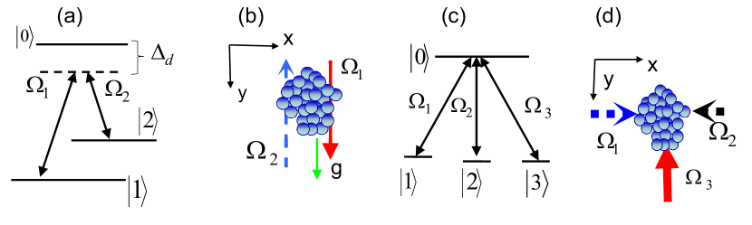
Figure 1: (Color online) Schematic of atom-laser interactions for artificial gauge potentials. (a) Three-level $\Lambda$-type atoms interacting with laser beams characterized by the Rabi frequencies $\Omega_{1}$ and $\Omega_{2}$ through the Raman-type coupling with a large single-photon detuning $\Delta_{d}$. (b) The configuration of the Raman laser beams for a spin Hall effect. (c) and (d) Atoms with tripod-level configuration interacting with three laser beams characterized by the Rabi frequencies $\Omega_{1}$, $\Omega_{2}$, and $\Omega_{3}$.

We may parameterize the Rabi frequencies through $\Omega_{1}=\Omega\text{sin}\theta e^{i\varphi}$ and $\Omega_{2}=\Omega\text{cos}\theta$, with $\Omega=\sqrt{|\Omega_{1}|^{2}+|\Omega_{2}|^{2}}$ ($\theta$ and $\varphi$ are in general spatially varying). We are interested in the subspace spanned by the two lowest dressed states $\left\{|\chi_{1}\rangle,|\chi_{2}\rangle\right\}$ (called respectively the dark and the bright states). This gives an effective spin-1/2 system, and in the spin language we also denote $|\chi_{\uparrow}\rangle\equiv|\chi_{1}\rangle$ and $|\chi_{\downarrow}\rangle\equiv|\chi_{2}\rangle$. In the case of a large detuning ($\Delta_{d}\gg\Omega$), both states $|\chi_{\uparrow}\rangle$ and $|\chi_{\downarrow}\rangle$ have negligible contribution from the initial excited state $|0\rangle$, so they are stable under atomic spontaneous emission. Furthermore, we assume the adiabatic condition, which requires that the off-diagonal elements of the matrices $\mathbf{\tilde{A}}$ and $\tilde{V}$ are much smaller than the eigenenergy differences $\left|\lambda_{i}-\lambda_{j}\right|$ ($i,j=1,2,0$) of the states $|\chi_{i}\rangle$. This gives the quantitative condition $\Delta_{D}\ll\Omega^{2}/\Delta_{d}$, where $\Delta_{D}=\text{cos}^{2}\theta|\mathbf{v}\cdot\nabla(\tan\theta e^{i\varphi})|$ ($\mathbf{v}$ is the typical velocity of the atom) represents the two-photon Doppler detuning [85]. Under this adiabatic condition, the effective Hamiltonian for the wave function $\Psi$ in the subspace spanned by $\left\{|\chi_{\uparrow}\rangle,|\chi_{\downarrow}\rangle\right\}$ is [84]

$$H_{\text{eff}}=\left(\begin{array}[]{cc}H_{\uparrow}&0\\ 0&H_{\downarrow}\end{array}\right),$$ (38)

where $H_{\sigma}=\frac{1}{2m}(-i\hbar\nabla-\mathbf{A}_{\sigma})^{2}+V_{\sigma}(\mathbf{r})$ $\left(\sigma=\uparrow,\downarrow\right)$. The gauge potentials $\mathbf{A}_{\sigma}$ can be obtained as $\mathbf{A}_{\uparrow}=-\mathbf{A}_{\downarrow}=-\hbar\text{sin}^{2}\theta\nabla\varphi,$ and the related gauge field

$$\mathbf{B}_{\sigma}=\nabla\times\mathbf{A}_{\sigma}=-\eta_{\sigma}\hbar\text{sin}(2\theta)\nabla\theta\times\nabla\varphi,$$ (39)

where $\eta_{\uparrow}=-\eta_{\downarrow}=1$. We obtain precisely a spin-dependent gauge field that is critical for the spin Hall effect. A typical scheme to generate atomic spin Hall effect is shown in Fig 1(b), which was demonstrated experimentally in Ref. [104].

Spin-orbit couplings in a tripod configuration. The second example we address is an $SU(2)$ non-Abelian gauge field created in a tripod-level configuration [93, 94, 95, 96]. Consider the adiabatic motion of atoms in $x$-$y$ plane with each having a tripod-level structure in a laser field as shown in Fig. 1(c) and (d). The atoms in three lower levels $|1\rangle$, $|2\rangle$ and $|3\rangle$ are coupled with an excited level $|0\rangle$ through three laser beams characterized by the Rabi frequencies $\Omega_{1}=\Omega\text{sin}\theta\mathrm{e}^{-i\kappa x}/\sqrt{2}$, $\Omega_{2}=\Omega\text{sin}\theta\mathrm{e}^{i\kappa x}/\sqrt{2}$, and $\Omega_{3}=\Omega\text{cos}\theta\mathrm{e}^{-i\kappa y}$, respectively, where $\Omega=\sqrt{|\Omega_{1}|^{2}+|\Omega_{2}|^{2}+|\Omega_{3}|^{2}}$ is the total Rabi frequency and the mixing angle $\theta$ defines the relative intensity. The atom-laser interaction Hamiltonian $H_{\text{AL}}$ in the interaction representation reads

$$H_{\text{AL}}=-\hbar\sum_{j=1}^{3}\Omega_{j}|0\rangle\langle j|+\mathrm{H.c.}.$$ (40)

Diagonalizing this Hamiltonian yields two degenerate dark states with zero energy as well as two bright states separated from the dark states by the energies $\pm\hbar\Omega$. If $\Omega$ is sufficiently large compared to the two-photon detuning due to the laser mismatch and/or Doppler shift, the adiabatic approximation is justified and one can safely study only the internal states of an atom evolving within the dark state manifold. In this case, the non-Abelian gauge potential $\mathbf{A}$ in the present configuration of the light field can be obtained as

$$\mathbf{A}=\hbar\kappa\left(\begin{array}[]{cc}\mathbf{e}_{y}&-\mathbf{e}_{x}\text{cos}\theta\\ -\mathbf{e}_{x}\text{cos}\theta&\mathbf{e}_{y}\text{cos}^{2}\theta\end{array}\right).$$ (41)

Furthermore, let the mixing angle $\theta=\theta_{0}$ with $\text{cos}\theta_{0}=\sqrt{2}-1$, such that $\text{sin}^{2}\theta_{0}=2\text{cos}\theta_{0}$. Thus, the vector potential takes a symmetric form $\mathbf{A}=\hbar\kappa^{\prime}(-\mathbf{e}_{x}\sigma_{x}+\mathbf{e}_{y}\sigma_{z})+\hbar\kappa_{0}\mathbf{e}_{y}I_{2},$ where $\kappa^{\prime}=\kappa\text{cos}\theta_{0}$ and $\kappa_{0}=\kappa(1-\text{cos}\theta_{0})$. Using a unitary transformation $\tilde{H}^{\prime}=U^{{\dagger}}\tilde{H}U$ with $U=\exp(-i\kappa_{0}y)\exp\left(-i\frac{\pi}{4}\sigma_{x}\right)$, one obtains the Hamiltonian for the atomic motion

$$H=\frac{1}{2m}[(p_{x}+\hbar\kappa^{\prime}\sigma_{x})^{2}+(p_{y}+\hbar\kappa^{\prime}\sigma_{y})^{2}]+V.$$ (42)

This Hamiltonian provides a coupling between the atomic center-of-mass motion and the internal pseudospin degrees of freedom, thus giving rise to an effective SOC.

However, the two degenerate dark states in this tripod configuration are not the lowest-energy states, so the atoms may quickly decay out of the dark states due to collisions and other relaxation processes. This problem may be solved by using the blue-detuned lasers [110] or a closed loop Raman coupling configuration [111]. Furthermore, the combination of an SOC and an effective perpendicular Zeeman field is required for the emergence of topological superfluid. To this end, five or two additional laser beams superposing into the above tripod configuration were proposed [112, 103]. However, locking the phases of these laser beams is challenging in experiments. It was thus proposed and then experimentally demonstrated that controlling polarizations of the Raman lasers is sufficient to generate simultaneously an effective SOC and a perpendicular Zeeman field for atoms [35, 113].

3.4.2 Laser-assisted tunneling

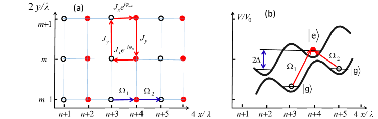
Figure 2: (Color online) Scheme for realizing artificial magnetic fields based on laser-assisted tunneling [114]. Open (closed) circles denote atoms in state $|g\rangle$ $(|e\rangle)$. (a) Hopping in the $y$-direction $J_{y}$ is the same for particles in states $|e\rangle$ and $|g\rangle$, while the $x$-direction hopping is laser-assisted. (b) Laser-assisted tunneling along the $x$-direction. Adjacent sites are set off by an energy $\Delta$. The laser $\Omega_{1}$ is resonant for transitions $|g\rangle$ and $|e\rangle$ while $\Omega_{2}$ is resonant for transitions $|e\rangle$ and $|g\rangle$ due to the offset of the lattice sites. The atoms hopping around one plaquette get phase shifts of $2\pi\alpha$ due to the created artificial magnetic fields.

Laser-induced tunneling was the first method proposed to generate artificial magnetic fields in OLs [114], and it was used to experimentally realize the Hofstadter-Harper model [48]. Furthermore, this method was further proposed to simulate artificial SOCs in OLs [115, 116, 117], and was implemented very recently in an experiment realizing artificial 2D SOC in a Raman OL [36]. In this section we illustrate the basic idea of laser-induced tunneling, following the original proposal in Ref. [114]. We then introduce recent developments in Sec. 4.

Consider a gas of atoms trapped in a 3D OL created by standing wave laser fields, which generates a potential for the atoms $V(\mathbf{r})=V_{0x}\text{sin}^{2}(kx)+V_{0y}\text{sin}^{2}(ky)+V_{0z}\text{sin}^{2}(kz)$ with $k=2\pi/\lambda$ being the wave vector of the light. We assume the lattice to trap atoms in two different internal hyperfine states $|e\rangle$ and $|g\rangle$ and the depth of the lattice in the $x-$ and $z-$directions to be so large that hopping in these directions due to kinetic energy is prohibited. Furthermore, we assume that adjusting the polarization of the lasers that confine the particles in the $x$-direction allows us to place the potential well trapping atoms in the different internal states at distances $\lambda/4$ with respect to each other, as shown in Fig. 2(a). Therefore, the resulting 2D lattice has a lattice constant (disregarding the internal state) in the $x$-direction of $a_{x}=\lambda/4$ and in the $y$-direction of $a_{y}=\lambda/2$. We focus on one layer of the OL in the $xy$-plane since in the following, there will neither be hopping nor interactions between different layers. The dynamics of atoms occupying the lowest Bloch band of this OL can be described by the Hamiltonian

$$H_{l}=\sum_{n,m}J_{y}(a^{\dagger}_{n,m}a_{n,m-1}+h.c.)+\sum_{n\in even,m}\omega_{eg}a^{\dagger}_{n,m}a_{n,m},$$

where $J_{y}$ is the hopping strength for particles to tunnel between adjacent sites along the $y$-direction. The energy difference between the two hyperfine states is $\omega_{eg}>0$ and the operators $a_{n,m}$ ($a^{\dagger}_{n,m})$ are destruction (creation) operators for atoms in the lowest motional band located at the site $x_{n,m}=(x_{n},y_{m})$, where $x_{n}=n\lambda/4$ and $y_{m}=m\lambda/2$.

In addition, there is an energy offset of $\Delta$ between two adjacent sites in the $x$-direction, as shown in Fig. 2(b). This can be achieved by accelerating the OL along the $x$-axis with a constant acceleration $a_{\text{acc}}$, which induces an additional potential energy term $H_{\text{acc}}=Ma_{\text{acc}}x$ with $M$ being the mass of the atoms. Alternatively, if both of the internal atomic states $|e\rangle$ and $|g\rangle$ have the same static polarizability $\mu$ an inhomogeneous static electric field of the form $E(x)=\delta Ex$, where $\delta E$ is the slope of the electric field in the $x$-direction, can be applied to the OL, which leads to a potential energy term $H_{\text{acc}}=\mu_{p}\delta Ex$. We keep this additional potential energy small compared to the OL potential and treat $H_{\text{acc}}$ as a perturbation. In second quantization this yields $H_{\text{acc}}=\Delta\sum_{n,m}na^{\dagger}_{n,m}a_{n,m}$, where $\Delta=\mu_{p}\delta E\lambda/4$ in the case of an inhomogeneous electric field and $\Delta=Ma_{\text{acc}}\lambda/4$ when the lattice is accelerated. The condition for this perturbation treatment to be valid is $\delta<<\nu_{x}$ with $\nu_{x}=4\sqrt{E_{R}V_{0x}}$ being the trapping frequency of the OL in the $x$-direction. Here $E_{R}=k^{2}/2M$ is the recoil energy.

Finally, the laser-induced tunneling can be activated along the $x$-direction by coupling two internal states $|g\rangle$ and $|e\rangle$ with two additional lasers forming Raman transitions. The Raman beams consist of two running plane waves chosen to give space-dependent Rabi frequencies of the form $\Omega_{1,2}=\Omega e^{\pm iqy},$ where $\Omega$ denotes the magnitude of the Rabi frequencies, and $\pm\Delta$ is the detuning. We assume the lasers not to excite any transitions to higher-lying Bloch bands with detuning of the order of $\Delta$, i.e. $\Omega\ll\Delta\ll\nu_{x}$. Then the lasers $\Omega_{1(2)}$ will only drive transitions $n-1\leftrightarrow n$ if $n$ is even (odd) and we can neglect any influence of the nonresonant transitions. Then one can find the following Hamiltonian describing the effect of the Raman lasers

$$H_{\text{AL}}=\sum_{n,m}(\gamma_{n,m}a^{\dagger}_{n,m}a_{n-1,m}+h.c.)-\sum_{n,m}\Delta a^{\dagger}_{n,m}a_{n,m}.$$

Here the matrix elements $\gamma_{nm}$ can be written as

$$\gamma_{n,m}=\frac{1}{2}e^{2i\pi\alpha m}\Omega\Gamma_{y}(\alpha)\Gamma_{x},$$

where $\alpha=q\lambda/4\pi$, and the matrix elements

$$\Gamma_{x}=\int dxw^{\star}(x)w(x-\lambda/4),\ \ \ \Gamma_{y}(\alpha)=\int dyw^{\star}(y)\text{cos}(4\pi\alpha m)w(y),$$

with $w(\mathbf{r})=w(x)w(y)w(z)$ being the Wannier function. To achieve a symmetric Hamiltonian, we assume hopping amplitudes $J_{x}=\Omega\Gamma_{x}\Gamma_{y}/2=J_{y}=J$, and thus the total Hamiltonian describing the configuration is given by

$$H_{\alpha}=J\sum_{n,m}\left(e^{2i\pi\alpha m}a^{\dagger}_{n,m}a_{n+1,m}+a^{\dagger}_{n,m}a_{n,m+1}+h.c.\right).$$

This Hamiltonian $H_{\alpha}$ is equivalent to the Hamiltonian for electrons with charge $e$ moving on a lattice in an external magnetic field $B=2\pi\alpha/A_{\text{cell}}e$, where $A_{\text{cell}}$ is the area of one elementary cell.

3.4.3 Periodically driven systems

Driving cold-atom systems periodically in time is a powerful method to engineer effective magnetic fields or SOCs, and thus can trigger topological quantum phases. For instance, the OL shaking method has been used to experimentally realize the Hofstadter model [118, 30, 29]. Modulating a honeycomb OL also led to the experimental realization of the Haldane model [28].

We first describe two simple examples to illustrate the basic concept of creating artificial gauge fields with the periodically driven method. In the first example we consider ultracold atoms trapped in a 1D shaken bichromatic OL [119]. This lattice is generated by the superposition of two shaken OLs. The single-particle Hamiltonian of an atom in this 1D shaken lattice system reads

$$H_{s}=\frac{p_{x}^{2}}{2m}+V_{1}\text{sin}^{2}[k_{1}(x-x_{1}(t))]+V_{2}\text{sin}^{2}[k_{2}(x-x_{2}(t)+\phi)],$$ (43)

where $V_{i}$, $k_{i}=2\pi/\lambda_{i}$, and $\lambda_{i}\ (i=1,2)$ are the lattice depth, laser wave vector and wavelength, respectively; and $\phi$ is the phase of the second laser, $x_{i}(t)=b\text{sin}(\omega t)$ is the periodic time-dependent lattice shaking. Here we assume that the two lattices experience the same shaking amplitude $b$ and frequency $\omega$. Experimentally, a shaking sinusoidal lattice can be realized through a modulation of the driving frequency and by changing the relative phase of the acousto-optic modulators. The tunneling between neighboring sites decreases exponentially with the intensity of the lasers creating the lattice, whereas the shape of the wavepacket (the Wannier functions) has a much weaker dependence. Therefore, by varying the laser intensity, one can rapidly vary the tunneling. With a unitary rotation, the Hamiltonian is transferred to a new frame $x\rightarrow x+b\text{sin}(\omega t)$

$$H_{r}=\frac{(p_{x}-A_{x})^{2}}{2m}+V_{1}\text{sin}^{2}(k_{1}x)+V_{2}\text{sin}^{2}(k_{2}x+\phi),$$ (44)

with a shaking-induced vector potential $A_{x}=m\omega\text{cos}(\omega t)$ [119].

The second example is the topological phases of a 2D honeycomb lattice proposed by Haldane [13], which can also be realized with the method of shaking lattices [28, 120]. We consider the following time-dependent lattice potential

$$V(x,y,t) =-V_{\overline{X}}\text{cos}^{2}[k_{r}(x+b\text{cos}\omega t)+\theta/2]-V_{{X}}\text{cos}^{2}[k_{r}(x+b\text{cos}\omega t)]$$

$$-V_{Y}\text{cos}^{2}[k_{r}(y+b\text{sin}\omega t)]-2\alpha\sqrt{V_{X}V_{Y}}\text{cos}[k_{r}(x+b\text{cos}\omega t)]\text{cos}[k_{r}(y+b\text{sin}\omega t)],$$

which leads to a honeycomb lattice realized by the ETH group when $b=0$ [77]. Here $\theta$ controls the energy offset between two sublattices $A$ and $B$ in the honeycomb lattice. The $b\not=0$ case describes a shaking lattice in both $x$ and $y$ directions with a phase difference $\pi/2$. Similar to the 1D case, transferring into the moving frame $x\rightarrow x+b\text{cos}(\omega t)$ and $y\rightarrow y+b\text{sin}(\omega t)$, one obtains a Hamiltonian with time-dependent vector potential term

$$H(t)=\frac{1}{2m}\left[\mathbf{p}-\mathbf{A}(t)\right]+V(x,y),$$ (46)

where $A_{x}(t)=m\omega b\text{sin}(\omega t)$ and $A_{y}(t)=-m\omega b\text{cos}(\omega t)$ [120]. It is equivalent to a Hamiltonian that describes a particle in an ac electrical field in the 2D plane $\mathbf{E}(t)=m\omega^{2}b(\text{cos}(\omega t),\text{sin}(\omega t))$. The phase diagram in this Hamiltonian has been calculated in Ref. [120], and it shows a similar phase diagram with that of the Haldane model [13]; i.e., it contains topological trivial and nontrivial phases characterized by a Chern number. This shaking lattice method has been experimentally used to realize the Haldane model [28], as addressed in detail in Sec. 4.2.3.

After addressing the basic ideas, we now turn to some general frameworks that describe periodically driven quantum systems. A general theoretical treatment of periodically driven quantum systems is based on the Floquet theory. For a periodically driven Hamiltonian ${H}(t)$ with period $\tau$, its Floquet operator ${\hat{F}_{o}}$ is defined as

$${\hat{F}_{o}}\equiv U(\tau_{i}+\tau,\tau_{i})=\mathcal{T}\exp\left[-i\int_{\tau_{i}}^{\tau+\tau_{i}}H(t)dt\right],$$ (47)

where $\tau_{i}$ is the initial time, and $\mathcal{T}$ denotes the required time-ordered integral as the Hamiltonian at different times do not necessarily commute. The eigenvalue and eigenstates of the Floquet ${\hat{F}_{o}}$ are given by

$${\hat{F}_{o}}|\varphi_{n}\rangle=e^{-i\epsilon_{n}\tau}|\varphi_{n}\rangle,$$ (48)

where $\epsilon_{n}\in(-\pi/\tau,\pi/\tau)$ is the quasi-energy. A general method to explore the topological phases, which is free from any further approximation, is to numerically evaluate Floquet operator $\hat{F}_{o}$ according to Eq. (47) and determine its eigenvalues and eigenfunctions from Eq. (48). If a periodically driven system exhibits nontrivial topology, there must be in-gap quasi-energies $\epsilon_{n}$ and their corresponding wave functions $\varphi$ are spatially well localized at the edge of the system [120].

A physically more transparent method is introducing a time-independent effective Hamiltonian $H_{\text{eff}}$ via the Floquet operator [120, 121]

$$U(\tau_{f},\tau_{i})=e^{-iK(\tau_{f})}e^{-i\tau H_{eff}}e^{iK(\tau_{i})},$$ (49)

where we impose that (1) $H_{\text{eff}}$ is a time-independent operator, (2) $K(t)$ is a time-periodic operator $K(t+\tau)=K(t)$ with zero average over one period, and (3) $H_{\text{eff}}$ does not dependent on the starting time $\tau_{i}$, which can be realized by transferring all undesired terms into the kick operator $K(\tau_{i})$. Similarly, $H_{\text{eff}}$ does not depend on the final time $\tau_{f}$. Equation (49) shows that the initial (final) phase of the Hamiltonian at time $\tau_{i}$ ($\tau_{f}$) may have an important impact on the dynamics. However, the topological phenomena in the periodically driven systems can be connected to those in equilibrium systems described by the effective Hamiltonian $H_{\text{eff}}$. Consider a static system described by a Hamiltonian $H_{0}$ that is driven by a time-periodic modulation $V(t)$, whose period $\tau=2\pi/\omega$ is assumed to be much smaller compared to any characteristic time scale in the problem. In this high-frequency regime, one can obtain the effective Hamiltonian by using a perturbation expansion.

We consider a time-periodic Hamiltonian $H(t)=H_{0}+V(t)$ with

$$V(t)=\sum_{j=1}^{\infty}[V^{(j)}e^{ij\omega t}+V^{(-j)}e^{-ij\omega t}]$$

between times $\tau_{i}$ and $\tau_{f}$, with the period of the driving $\tau=2\pi/\omega$. The time-dependent potential has been explicitly expanded with its Fourier’s form. By using a perturbation expansion in powers of $1/\omega$, one can obtain [121]

$$H_{\text{eff}} = H_{0}+\frac{1}{\omega}\sum_{j=1}^{\infty}\{\frac{1}{j}[V^{(j)},V^{(-j)}]$$ (50)

$$+ \frac{1}{2\omega^{2}}([[V^{(j)},H_{0}],V^{(-j)}]+[[V^{(-j)},H_{0}],V^{(j)}]\}+\mathcal{O}(\tau^{3}),$$

$$K(t) = \int^{t}V(t^{\prime})dt^{\prime}+\mathcal{(}\tau^{2}).$$ (51)

In Eq. (50), the second-order terms that mix different harmonics have been omitted.

To understand the emergence of topological nontrivial phases, we usually write the Hamiltonian into momentum space. As for two-band systems, the general Hamiltonian in momentum space $\mathbf{k}$ can be rewritten as $H_{\text{eff}}=\mathbf{B}(\mathbf{k})\cdot\mathbf{\sigma}$. By using this kind of perturbation expansion, one can obtain the explicit expressions of $\mathbf{B}(\mathbf{k})$ for the models described in Eqs. (43) and (3.4.3) [119, 120], which shows that the nontrivial topological phases can be induced in the periodically driven OLs.

The perturbation expression in Eq. (50) can also be used in the derivation of the effective Hamiltonian for the general situation where a pulse sequence is characterized by the repeated $N$-step sequence

$$\gamma_{N}=\{H_{0}+V_{1},H_{0}+V_{2},\cdots,H_{0}+V_{N}\},$$ (52)

where the $V_{m}$’s are arbitrary operators [121]. For simplicity, we assume that the duration of each step is $\tau/N$, and we further impose that $\sum_{m=1}^{N}V_{m}=0$. The Hamiltonian $\gamma_{N}$ can be expanded in terms of the harmonics $H(t)=H_{0}+\sum_{j\not=0}V_{j}e^{ij\omega t},$ where

$$V_{j}=\frac{1}{2\pi i}\sum_{m=1}^{N}\frac{1}{j}e^{-i2\pi jm/N}(e^{ij(2\pi/N)}-1)V_{m}.$$

By applying Eqs. (50) and (51), one can derive the effective Hamiltonian and the initial-kick operator as

$$H_{\text{eff}} = H_{0}+\frac{2\pi i}{N^{3}\omega}\sum_{m<n=2}^{N}\mathcal{C}_{m,n}[V_{m},V_{n}]+\frac{\pi^{2}(N-1)^{2}}{6N^{4}\omega^{2}}\sum_{m=1}^{N}[[V_{m},H_{0}],V_{m}]$$ (53)

$$\ \ \ +\frac{\pi^{2}}{6N^{4}\omega^{2}}\sum_{m<N=2}^{N}\mathcal{D}_{m,n}\left([[V_{m},H_{0}],V_{n}]+[[V_{n},H_{0}],V_{m}]\right)+\mathcal{O}(1/\omega^{3}),$$

$$K(0) = \frac{2\pi}{N^{2}\omega}\sum_{m=1}^{N}mV_{m}+\mathcal{O}(1/\omega^{2}),$$ (54)

where $\mathcal{C}_{m,n}=N/2+m-n$ and $\mathcal{D}_{m,n}=1+N^{2}-6N(n-m)+6(n-m)^{2}$. The above equations show that the initial kick $K(0)$ depends on the way the pulse sequence starts, whereas the effective Hamiltonian $H_{\text{eff}}$ is independent of this choice: redefining the operators $V_{m}\rightarrow V_{m+j}$ with an integer $j$ results in a change in $K(0)$ but leaves $H_{\text{eff}}$ invariant. The expressions are useful for engineering effective Hamiltonians with artificial gauge fields. In view of this fact, we illustrate the case $N=4$ in the following.

Consider the following four-step sequence:

$$\gamma_{4}=\{{H}_{0}+{L_{1}},{H}_{0}+{L_{2}},{H}_{0}-{L_{1}},{H}_{0}-{L_{2}}\},$$ (55)

we obtain

$${H}_{\text{eff}} = {H}_{0}+\frac{i\pi}{8\omega}[{L_{1}},{L_{2}}]+\frac{\pi^{2}}{48\omega^{2}}\left([[{L_{1}},H_{0}],{L_{1}}]+[[{L_{2}},H_{0}],{L_{2}}]\right)+\mathcal{O}(1/\omega^{3}),$$ (56)

$${K}(0) = -\frac{\pi}{4\omega}({L_{1}}+{L_{2}})+\mathcal{O}(1/\omega^{2}).$$ (57)

We first consider atoms moving in a two-dimensional free space, such that ${H}_{0}=({p}_{x}^{2}+{p}_{y}^{2})/2m$. We drive the system with a pulse sequence (55) with the operator

$${L_{1}}=({p}_{x}^{2}-{p}_{y}^{2})/2m,\ \ {L_{2}}=\kappa{x}{y}.$$

The corresponding effective Hamiltonian is given by Eq. (56), which yields, up to the second order $(1/\omega^{2})$

$${H}_{\text{eff}}=\frac{1}{2m}[({p}_{x}-A_{x})^{2}+({p}_{y}-A_{y})^{2}]+\frac{m\omega_{h}^{2}}{2}({x}^{2}+{y}^{2}),$$

where $\mathbf{A}=(A_{x},A_{y})=(-m\Omega y,m\Omega x)$ with $\Omega=\pi\kappa/(8m\omega)$ and $\omega_{h}=\sqrt{5/3}\Omega$. It corresponds to the realization of a perpendicular and uniform artificial magnetic field $\mathbf{B}=2m\Omega\mathbf{e}_{z}=\pi\kappa/(4\omega)\mathbf{e}_{z}$. An early version of this scheme for artificial magnetic fields was proposed to realize fractional QHE with bosonic atoms in OLs [122].

The similar four-step sequence can also be used to generate SOCs. Considering the operators ${H}_{0}=({p}_{x}^{2}+{p}_{y}^{2})$ and

$${L_{1}}=({p}_{x}^{2}-{p}_{y}^{2}),\ \ {L_{2}}=\kappa({x}\sigma_{x}-{y}\sigma_{y}).$$

The time evolution of the driven system is characterized by the effective Hamiltonian

$${H}_{\text{eff}}=\frac{{p}_{x}^{2}+{p}_{y}^{2}}{2m}+\lambda_{R}(\sigma_{x}{p}_{x}+\sigma_{y}{p}_{y})+\Omega_{SO}{L}_{z}\sigma_{z}+\mathcal{O}(1/\omega^{3}),$$ (58)

where $\lambda_{R}=\pi\kappa/(8m\omega)$ and $\Omega_{SO}=-(8m/3)\lambda_{R}^{2}$. The term ${H}_{R}=\lambda_{R}{\mathbf{p}}\cdot\mathbf{\sigma}$ is the Rashba SOC, and ${H}_{L\sigma}=\Omega_{SO}{L}_{z}\sigma_{z}$ is the so-called ”intrinsic” or ”helical” SOC, which is responsible for the quantum spin Hall effect in topological insulators. The combination of these two terms appears in the Kane-Mele model (see Sec. 4.2.4).

4 Topological quantum matter in optical lattices

In the previous section, we introduced the techniques for engineering the Hamiltonian of cold atoms, specially the techniques of creating artificial magnetic fields and SOCs. The use of these techniques in OLs has led to the realization and characterization of some topological states for cold atoms. Compared with conventional solid-state systems, cold atoms offer an ideal platform with great controllability to study topological models. For instance, the laser fields that couple hyperfine states of atoms can be used to synthesize effective physical fields, such as gauge fields, SOCs, and Zeeman fields. The forms and strengths of those synthetic fields are tunable as they are determined by the atom-laser coupling configurations. The structure of an OL can be designed via several counterpropagating lasers to realize various unconventional lattice potentials, which include the double-well superlattices, honeycomb lattices, spin-dependent lattices, and so on.

This section systematically discusses some important lattice models with topological quantities originally introduced in condensed matter theories and describes their proposed schemes as well as current implementation methods. The topological bands and phenomena in these models can be created and detected with cold atoms in OLs. These lattice models range from 1D to 3D and even higher-dimension geometries, which can be implemented with OLs of various geometric structures. These systems mainly focus on energy bands in the absence of interactions, and hence the topological phenomena addressed here correspond to the single-particle physics. Some advances in their extension to the interacting regime will also be briefly discussed.

This section is divided into five parts. In the first, we describe some basic topological models with nontrivial bands realized in 1D OLs, which include the famous Su-Schrieffer-Heeger (SSH) model and its implementation for topological pumping. In the second part we discuss the physics of Dirac fermions, the topological properties of the Hofstadter model, Haldane model and Kane-Mele model, and their experimental realization and detection in 2D OLs. Some typical 3D topological insulating states of $\mathbb{Z}_{2}$ or $\mathbb{Z}$ types and topological gapless (semimetal) states with emergent Dirac or Weyl fermions in 3D OLs are presented in the third part. The last two parts are respectively devoted to topological states in higher dimensions with the newly developed synthetic dimension technique and unconventional topological quasi-particles with higher pseudospins for cold atoms in OLs, both of which are currently absent or extremely challenging to realize in condensed matter systems.

4.1 One-dimension

4.1.1 Su-Schrieffer-Heeger model and Rice-Mele model

The SSH model [3, 4] for polyacetylene is the simplest 1D model of band topology in condensed matter physics. Such a model describes the polyacetylene with free fermions moving in a 1D chain with dimerized tunneling amplitudes. The essence of the SSH model is manifested by two topological characters. The first character is the nontrivial Zak phase that describes distinct topological phases in 1D lattice systems with zero-energy edge modes in a finite chain with open boundaries. The second one is the topological solitons with fractional particle numbers, which emerge on the domain walls in the lattice potential to separate two dimerization structures. The physics of such a dimerized lattice with two sites per unit cell is captured by the SSH Hamiltonian

$$H_{\text{SSH}}=-\sum_{n}(Ja_{n}^{{\dagger}}b_{n}+J^{\prime}a_{n}^{{\dagger}}b_{n-1}+h.c.),$$ (59)

where $J$ and $J^{\prime}$ denote the modulated hopping amplitudes, and $a_{n}^{{\dagger}}$($b_{n}^{{\dagger}}$) are the creation operators for a particle on the sublattice site $a_{n}$($b_{n}$) in the $n$th lattice cell, as shown in Fig. 3(a). Written in momentum space, the Hamiltonian (59) takes the form $H_{\text{SSH}}=\sum_{k}\Psi_{k}^{{\dagger}}\mathcal{H}_{\text{SSH}}(k)\Psi_{k}$ with $\Psi_{k}^{{\dagger}}=\left(a_{k}^{{\dagger}},b_{k}^{{\dagger}}\right)$ and

$$\mathcal{H}_{\text{SSH}}(k)=-[J+J^{\prime}\text{cos}(ka)]\sigma_{x}-J^{\prime}\text{sin}(ka)\sigma_{y},$$ (60)

where $a$ denotes the lattice spacing. Consequently, there are two bands with the energy dispersion $E_{\pm}=\pm\sqrt{[J+J^{\prime}\text{cos}(ka)]^{2}+[J^{\prime}\text{sin}(ka)]^{2}}$.

It can be found that $\mathcal{H}_{\text{SSH}}(k)$ possesses the chiral symmetry $\sigma_{z}\mathcal{H}_{\text{SSH}}(k)\sigma_{z}=-\mathcal{H}_{\text{SSH}}(k)$ and the TRS $\hat{T}\mathcal{H}_{\text{SSH}}(k)\hat{T}^{-1}=\mathcal{H}_{\text{SSH}}(-k)$, where $\hat{T}=\hat{\mathcal{K}}$ with $\hat{\mathcal{K}}$ being the complex conjugate operator. Note that the chiral symmetry here is a sublattice symmetry and requires that hoppings only exist between two sublattices. The chiral symmetry gives rise to an additional particle-hole (charge-conjugation) symmetry because for any eigenstate $|u_{E}\rangle$ with energy $E$ there exists a corresponding eigenstate $|u_{-E}\rangle=\sigma_{z}|u_{E}\rangle$ with energy $-E$. Thus, the SSH model is classified in the BDI class of topological insulators [123]. It is known that the SSH model has two topologically distinct phases with different dimerization configurations, $D1$ for $J>J^{\prime}$ and $D2$ for $J<J^{\prime}$, separated by a topological phase transition point at $J=J^{\prime}$. The topological features can be characterized by the Zak phase [62]

$$\varphi_{Zak}=i\int^{G/2}_{-G/2}\langle u_{\pm}(k)|\partial_{k}|u_{\pm}(k)\rangle dk,$$ (61)

where $G=2\pi/d$ is the reciprocal lattice vector with $d=2a$ and $|u_{\pm}(k)\rangle$ denote the Bloch wave functions of the higher ($+$) and lower ($-$) bands. The Zak phase in each lattice configuration is a gauge dependent quantity depending on the choice of origin of the unit cell. For our choice, the Zak phase $\varphi_{Zak}=0$ for $D1$ and there is no edge state, yielding a trivial insulating phase. For $D2$, $\varphi_{Zak}=\pi$ and the system hosts two degenerate zero-energy edge states, yielding a gapped topologically nontrivial phase. The difference between the Zak phases for the two dimerization configurations is well defined as $\delta\varphi_{Zak}=\pi$, which is gauge invariant and thus can be used to identify the different topological characters of the Bloch bands. In the topologically nontrivial phase, there are two degenerate zero-energy modes respectively localized at two edges of the system under the open boundary condition.

Another topological feature in the SSH model is that a kink (anti-kink) domain between the two dimerization configurations gives rise to an undegenerate, isolated soliton (anti-soliton) state on the domain, which is a zero-energy mid-gap state. Due to the particle-hole ambiguity of the energy spectrum, the zero mode takes the fractional fermion number $\mathcal{N}=\frac{1}{2}$ ($\mathcal{N}=-\frac{1}{2}$) when this mode is occupied (unoccupied). The soliton state is topologically protected in the sense that it is impossible to remove it without closing the bulk energy gap, which is due to the fact that it is on an interface between topologically distinct phases. Historically, such topological solitons with fractional particle numbers were first found in a 1D modified Dirac equation in the context of the field theory by Jackiw and Rebbi [124] (see Sec. 6.1), and the SSH model provides the first physical demonstration of this remarkable phenomenon in lattice systems.

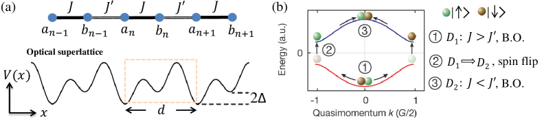
Figure 3: (Color online) (a) Schematic illustration of the 1D optical superlattice for realizing the SSH model ($\Delta=0$) and the Rice-Mele model ($\Delta\neq 0$) in the experiment [125]. The yellow box denotes the unit cell containing two sites with staggered hopping strengths ($J$ and $J^{\prime}$) and tunable energy offset (2$\Delta$). (b) Schematic illustration of experimental three-step sequence of measuring the Zak phase difference $\delta\varphi_{Zak}$, based on a combination of spin-dependent Bloch oscillation (B.O.) and Ramsey interferometry [125]. The preparation and state evolution of the atomic gas in a superposition of two spin-states with opposite magnetic moment (brown and green balls) are described in the text.

The SSH model was generalized to describe the linearly conjugated diatomic polymers with the Rice-Mele Hamiltonian [126]

$$H_{\text{RM}} = -\sum_{n}(Ja_{n}^{{\dagger}}b_{n}+J^{\prime}a_{n}^{{\dagger}}b_{n-1}+h.c)+\Delta\sum_{n}(a_{n}^{{\dagger}}a_{n}-b_{n}^{{\dagger}}b_{n}),$$ (62)

where $\Delta$ is the energy offset between neighboring lattice sites. For a heteropolar dimer configuration with $\Delta\neq 0$, the particle-hole symmetry (and chiral symmetry) in the original SSH model is broken. Consequently, the Zak phase is fractional in units of $\pi$ and depends on the energy offset $\Delta$. Strictly, the Rice-Mele model is not topological in the theory of topological classification with symmetry [61]. However, one can investigate the existence of edge modes to determine which configuration has nontrivial properties in this case, noting that the two edge modes in the topological phase are no longer degenerate when $\Delta\neq 0$. If there is a domain wall in the Rice-Mele model, where a Dirac Hamiltonian emerges in the continuum limit as the generalized Jackiw-Rebbi model (see Sec. 6.1), the unpaired soliton state in general has non-zero energy and carries an irrational particle number [126, 127, 128]. The Rice-Mele/SSH model with band topology (geometry) provides a paradigmatic system for studying topological quantum pumps [129, 130, 131] (see Sec. 4.1.2).

Compared with conventional solid-state materials, cold atom systems offer a perfectly clean platform with high controllability to study topological states of matter. The first scheme to simulate the SSH/Rice-Mele model along this direction was proposed to engineer the spatial profiles of the hopping amplitudes for cold atoms in a 1D optical superlattice in such a way that an optically induced defect as the domain wall carries fractional particle numbers in the lattice [132, 133, 134]. In the proposed system, a two-species gas of fermionic atoms is trapped in a state-dependent OL, where the internal states are denoted by $|\uparrow\rangle$ and $|\downarrow\rangle$. The two atomic species experience different optical potentials that are shifted relative to each other by $\lambda/4$, where $\lambda$ is the wavelength of light of the confining OL. Such a state-dependent OL is achieved when the laser beam is blue detuned from the internal transition of the atoms in $|\uparrow\rangle$ and red detuned by the same amount from the internal transition of the atoms in $|\downarrow\rangle$. When the lattice is sufficiently deep, each site is assumed to support one mode function that is weakly coupled to two nearest-neighbor sites, such that the hopping of the atoms between adjacent lattice sites only occurs as a result of driving by coherent electromagnetic fields. The coupling could be a far-off-resonant optical Raman transition via an intermediate atomic level. In this way, the required dimerized OL with the alternating hopping for atoms can be realized by using coupling lasers of proper two-photon Rabi frequency. Since the laser phase directly modulates the hopping configuration, when there is a jump in one particular lattice site in the laser phase, it will generate a domain wall to separate the $D1$ and $D2$ configurations [132]. The topological soliton states in the domain wall in this OL system are tunable via the atom-laser coupling parameters. A similar proposal based on a 1D spin-dependent OL for synthesizing SSH/Rice-Mele models with fully tunable parameters in the absence of domains was also presented in Ref.[135].

Creation and measurement of the fractionalized soliton modes in the domain walls are experimentally challenging. It was suggested that the fractional particle number could be detected via far-off-resonant light scattering in the atomic gases trapped in OLs [133, 134]. By measuring the intensity of the scattered light, one can detect the fractional expectation value of the atom number and its fluctuations. It was recently demonstrated that the fractional particle number in the SSH/Rice-Mele model can be simulated in the momentum-time parameter space in terms of Berry curvature without a spatial domain wall [136]. In the simulation, a hopping modulation is adiabatically tuned to form a kink-type configuration, and the induced current plays the role of an analogous soliton distributing in the time domain. Thus the mimicked fractional particle number is expressed by the particle transport and can be detected from the center-of-mass motion of an atomic cloud. Two feasible experimental setups of OLs for realizing the required SSH Hamiltonian with tunable parameters and time-varying hopping modulation were presented in Ref. [136].

Other schemes for creating 1D topological bands and soliton/edge states have recently been proposed by using cold atoms trapped in double-well OLs. The authors in Ref. [137] considered a single species of fermionic atoms occupying an $sp$ orbital ladder of the two wells, where the staggered hopping pattern for realizing the topological phase naturally arises. In the noninteracting limit, the $sp$ orbital ladder naturally reproduces the SSH model with a quantized Zak phase and fractionalized zero-energy edge states. The stability of the topological phase against atomic interactions and the emergence of topological flat bands of edge modes in the presence of inter-ladder coupling were also discussed [137]. It was shown that an atomic gas of attractively interacting fermions in a 1D periodically shaken OL can give rise to the emergent Rice-Mele model with controlled domain walls, which comes from the density-wave ground state [138]. By using cold atoms in a spin-dependent optical double-well lattice, one may realize a two-leg generalized SSH model with glide reflection symmetry [139], which is topologically characterized by Wilson lines and automatical fractionalization without producing domains in the lattice due to the interplay between the glide symmetry and atomic repulsive interactions.

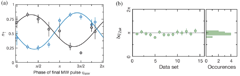
Figure 4: (Color online) Determination of the Zak phase. (a) The atom number in the two spin states $N_{\uparrow,\downarrow}$ is measured following the sequence and the fraction of atoms in the $|\!\!\uparrow\rangle$ spin state $n_{\uparrow}=N_{\uparrow}/(N_{\uparrow}+N_{\downarrow})$ is plotted as a function of the phase of the final microwave $\pi/2$-pulse. The difference in the phases of the two Ramsey fringes yields the Zak phase difference $\delta\varphi_{\text{Zak}}$. Blue (black) circles correspond to the fringe in which the dimerization was (not) swapped. (b) Measured relative phases for 14 identical experimental runs (left), which give an average value of $\delta\varphi_{\text{Zak}}=0.97(2)\pi$. The corresponding histogram is shown on the right with a binning of $0.05\pi$. Reprinted by permission from Macmillan Publishers Ltd: Atala et al.[125], copyright© (2013).

The SSH/Rice-Mele model described by the Hamiltonian (62) with the tunable energy offset $\Delta$ has already been experimentally realized with a Bose-Einstein condensate (BEC) of ⁸⁷Rb trapped in a 1D optical superlattice [125]. The superlattice potential shown in Fig. 3(a) is created by superimposing two standing optical waves of short- and long-wavelengths differing by a factor of two ($\lambda_{l}=2\lambda_{s}=1534$nm), which leads to the total lattice potential $V(x)=V_{l}\text{sin}^{2}(k_{L}x+\phi/2)+V_{s}\text{sin}^{2}(2k_{L}x+\pi/2)$, where $k_{L}$ is the wave vector of the short wavelength trapping lasers, and $V_{1}$ and $V_{s}$ are the corresponding strengths of the two standing waves. The lattice potential can be controlled by varying the laser intensity of long-wavelength standing-wave lasers to make the system well described by the SSH/Rice-Mele Hamiltonian in the tight-binding regime. Phase control between the two standing wave fields enables one to fully control $\phi$ for tuning the atomic hopping. This makes the OL into the $D1$ or $D2$ configuration with ease. In the experiment, switching between $\phi=0$ and $\phi=\pi$ was used to rapidly access the two different dimerized configurations with $\Delta=0$, whereas a tunable energy offset $\Delta\neq 0$ was also introduced by tuning $\phi$ slightly away from these symmetry points.

Moreover, the Zak phase $\delta\varphi_{Zak}$ characterizing the topological Bloch bands was detected, even though the atoms used in the experiment are bosons. A three-step sequence shown in Fig. 3(b) was employed, which is based on a combination of spin-dependent Bloch oscillations and Ramsey interferometry [125]. The first step is to start with an atomic condensate in the state $|\downarrow,k=0\rangle$ and bring it into a coherent superposition state $1/\sqrt{2}(|\uparrow,k=0\rangle+|\downarrow,k=0\rangle)$ using a microwave $\pi/2$-pulse. Here $\sigma=\uparrow,\downarrow$ denotes two spin states of the atoms with opposite magnetic moment and $k$ is the central momentum of the condensate. Then a magnetic field gradient is applied to create a constant force in opposite directions for the two spin components, leading to spin-dependent Bloch oscillations. In this process, the atomic wavepacket evolves into the coherent superposition state $1/\sqrt{2}(|\uparrow,k\rangle+e^{i\delta\varphi}|\downarrow,-k\rangle)$. When the two states reach the band edge, the differential phase between them is given by $\delta\varphi=\varphi_{Zak}+\delta\varphi_{\text{Zeeman}}$, where $\delta\varphi_{\text{Zeeman}}$ denotes the Zeeman phase difference induced by the magnetic field. For the TRS Hamiltonian here, the dynamical phase acquired during the adiabatic evolution is equal for the two spin states and thus cancels in the total phase difference. The second step is to eliminate the Zeeman phase difference by applying a spin-echo $\pi$-pulse and switching dimerization configurations following the first step. For atoms located at the band edge $k=\pm G/2$, this non-adiabatic dimerization switch induces a transition to the upper band of the SSH/Rice-Mele model. The sequence is finally completed by letting the spin components further evolve in the upper band until they return to the band center $k=0$. At this point, a final $\pi/2$-pulse with phase $\varphi_{MW}$ is applied in order to make the two spin components interfere and read out their relative phase $\delta\varphi_{Zak}$ through the resulting Ramsey fringe. Experimental results for the two Ramsey fringes obtained with and without dimerization swapping during the state evolution are shown in Fig. 4(a), and the obtained phase differences are shown in Fig. 4(b), together with the corresponding histogram. Thus, the Zak phase difference between the two dimerized configurations was determined to be $\delta\varphi_{\text{Zak}}=0.97(2)\pi$, which agrees well with theoretical prediction of the topological Bloch bands in the SSH model. This method was used to further study the dependence of the Zak phase on the offset energy $\delta\varphi_{\text{Zak}}(\Delta)$, which corresponds to the Rice-Mele model with the fractional Zak phase. This work establishes a general approach for probing the topological invariant in topological Bloch bands in OLs. The measurement technique can be extended to more complicated topological models, such as detecting the Chern numbers of the Hofstadter model and the Haldane model [48, 28], and the $\pi$ Berry flux associated with a Dirac point in 2D OL systems [140].

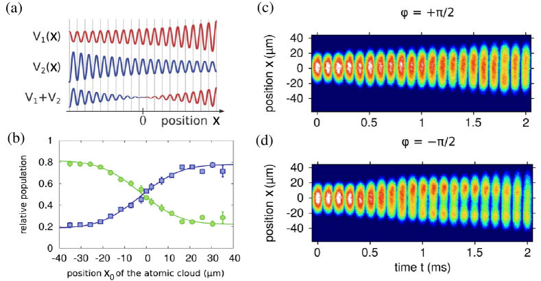
Figure 5: (Color online) Realizing the interface and probing the topological bound state from temporal evolution of atomic clouds. (a) The 1D OL with spatially varying lattice depth from the amplitude-chirped lattice potentials $V_{1,2}(x)$, which increases (decreases) along $x$ for positive (negative) values of the Raman detuning. (b) Measured spatial variation of band ordering. Relative atomic population transferred into the upper (green circles) and lower (blue squares) band on loading from an initial state with an atomic cloud centered at position $x_{0}$. Series of absorption images for a relative phase of the initially prepared atomic wavepacket of (c) $\varphi=+\pi/2$ and (d) $\varphi=-\pi/2$ for different holding times in the lattice. For $\varphi=+\pi/2$, trapping of atoms in the topological edge state was observed, while for $\varphi=-\pi/2$, the cloud splits up. Reprinted with permission from Leder et al. [141].

After measuring the bulk topological index in the SSH model, cold atom experiments have begun to probe topological boundary states at the intersection of two different topological phases. Recently, two different approaches for synthesizing and observing topological soliton states in the SSH model using BECs in 1D OLs were experimentally developed [141, 142]. In the first experiment [141], the authors used a 1D OL for cold rubidium atoms with a spatially chirped amplitude to create a domain wall and then directly observed the soliton state by optical real-space imaging of atoms confined at the interface. The lattice potential is realized using a rubidium atomic three level configuration with two ground states of different spin projections and one excited state. To achieve a topological interface, two four-photon potentials $V_{1}(x)$ and $V_{2}(x)$ with opposite spatial variation of the Raman coupling are superimposed, as shown in Fig. 5(a). This gives rise to a 1D lattice potential $V(x)=V_{1}(x)+V_{2}(x)\approx 2a\cdot x\text{cos}(4k_{L}x)$, creating a zero crossing at $x=0$, where $k_{L}=2\pi/\lambda$ with $\lambda$ being the wavelength of the laser beams. For $x>0$ ($x<0$) the maxima (minima) of the potential are located at integer multiples of $\lambda/4$, This phase change is reflected in the inversion of ordering bands, which cannot be transformed into each other by continuous deformation without closing the gap. For such a situation a non-degenerate topologically protected bound state localized around $x=0$, where the bands intersect, is expected in the SSH model. The dynamics of atoms in such a structure near the band crossing is described by the Dirac Hamiltonian with a spatially dependent effective mass (the Jackiw-Rebbi model) in the continuum limit with good accuracy, as the width of the topological bound state is two orders of magnitude larger than the lattice spacing [141]. To verify the band inversion on sign change of $x$, the adiabatically expanded atomic cloud centered at different lateral positions $x_{0}$ along the lattice beam axis was transferred to the state $\phi_{\text{i}}(x)=\frac{1}{\sqrt{2}}\phi_{x}(x-x_{0})(e^{2ikx}+e^{-2ikx})$ via two simultaneously performed Bragg pulses. The band populations following activation of the lattice were determined. For $x<0$, loading is enhanced in the lower band, while for $x>0$ most atoms are transferred into the upper band, and near $x=0$ the curves cross, as shown in Fig. 5(b). This experimentally verifies the spatial variation of the band structure and the exhibition of a topological interface at $x=0$. Next in the experiments, the atoms were loaded into the interface and the topological bound state was observed via an initial state $\phi_{\text{i}}(x)=\frac{1}{\sqrt{2}}\phi_{x}(x)(e^{2ikx}+e^{-i\varphi}e^{-2ikx})$ with $\varphi=\pi/2$. The atomic wavepacket was centered at $x=0$, after which the lattice beams were activated and a series of atomic absorption images were recorded after a variable holding time in Fig. 5(c). This shows that the atomic cloud remains trapped at the expected position of the topological bound state. On the other hand, for a phase of $\varphi=-\pi/2$, no such trapping in the bound state was observed, as shown in Fig. 5(d). As expected, there is no overlap with the topological bound state when the initially prepared atomic wavepacket is $\pi$ out of phase, such that the wavepacket is split into two spatially diverging paths. Further evidence for the successful population of the topological bound state was obtained from the phase ($\varphi$) dependence and the dependence of the initial atomic momentum width on loading efficiency.

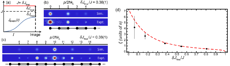
Figure 6: (Color online) Adiabatic preparation of the topological bound state in the momentum-space lattice. (a) Time sequence of the smooth ramp of the weak tunneling links (blue), holding the strong (red) links fixed. (b) Simulated (top) and averaged experimental (bottom) absorption images for an adiabatically loaded edge-defect lattice. (c) Same as (b), but for an adiabatically loaded central-defect lattice. (d) Decay length of the atomic distribution on even sites of the edge-defect lattice vs. $\delta J_{\text{final}}/J$. The dashed line represents the results of a numerical simulation of the experimental sequence. Reprinted with permission from Meier et al.[142].

In another experiment [142], a momentum-space lattice was used to simulate the hard-wall boundaries in the SSH model and the simulated topological bound state was then observed by site-resolved detection of the populations in the lattice. The physics of the SSH lattice model was emulated by using the controlled evolution of momentum-space distributions of cold atomic gases [143, 144]. Controlled coupling between discrete free-particle momentum states is achieved through stimulated two-photon Bragg transitions, driven by counterpropagating laser fields detuned far from atomic resonance. The lasers coherently coupled 21 discrete atomic momentum states in the experiment [142], creating a ”momentum-space lattice” of states in which atomic population may reside [see, e.g., Figs. 6(b,c)]. The momentum states are characterized by site indices $n$ and momenta $p_{n}=2n\hbar k_{L}$. The coupling between these states is fully controlled through 20 distinct two-photon Bragg diffraction processes, allowing simulation of 1D tight-binding models with local control of all site energies and tunneling terms. This enables one to create the hard-wall boundaries and lattice defects in the SSH model. The authors then directly probed the topological bound states in the SSH model simulated in such an OL through quench dynamics, phase-sensitive injection, and adiabatic preparation. The first detection method is to abruptly expose the condensate atoms initially localized at only a single lattice site and observe the ensuing quench dynamics with single-site resolution. When population was injected onto a defect site, a large overlap with the topological bound state was found, resulting in a relative lack of dynamics as compared to injection at any other lattice site. The second method is to probe the inherent sensitivity of the bound state to a controlled relative phase of initialized states, following a Hamiltonian quench. It was observed that the dynamics is nearly absent when the phase matches that of the bound state, while defect-site population is immediately reduced when the phase does not match. Lastly, the topological mid-gap bound state was directly probed through a quantum annealing procedure. The bound eigenstate was initially prepared in the fully dimerized limit of the time-dependent SSH Hamiltonian [142]

$$H_{\text{SSH}}(t)=-\sum_{n\in\text{odd}}{(J+\delta J_{\text{final}})(c^{\dagger}_{n+1}c_{n}+\text{h.c.})}-\sum_{n\in\text{even}}{J_{\text{even}}(t)(c^{\dagger}_{n+1}c_{n}+\text{h.c.})}\ ,$$ (63)

with only the odd tunneling links present at a strength $J_{\text{odd}}=J+\delta J_{\text{final}}$. Atomic population was injected at the decoupled zeroth site, identically overlapping with the mid-gap state. Next, the tunneling on the even links was slowly increased from zero to $J-\delta J_{\text{final}}$, as depicted by the smooth ramp in Fig. 6(a). For adiabatic ramping, the atomic wavefunctions should follow the eigenstate of $H_{\text{SSH}}(t)$. This adiabatic preparation method was performed for a lattice with the defect on the left edge and at its center, as shown in Fig. 6(b) and 6(c), respectively. As known in the SSH model, the amplitude of the mid-gap state wavefunction is largest at the defect site and decays exponentially into the bulk. The decay length $\xi$ (in units of the spacing between lattice sites) should scale roughly as the inverse of the energy gap. Thus, highly localized mid-gap states for $\delta J_{\text{final}}/J\sim 1$ (dimerized limit) and full delocalization over all 21 sites for $\delta J_{\text{final}}/J\ll 1$ (uniform limit) are expected. By tuning the normalized tunneling imbalance in the experiment, one can achieve a direct exploration of the mid-gap state’s localization decay length as a function of $\delta J_{\text{final}}/J$, as shown in Fig. 6(d). The technique of creating momentum-space lattices with direct and full control of tunneling configuration demonstrated in this work has been extended to create 2D artificial flux lattices for cold atoms [145].

4.1.2 Topological pumping

Quantum pumping as originally proposed by Thouless  [129] entails the transport of charge in a 1D periodic potential through an adiabatic cyclic evolution of the underlying Hamiltonian. In contrast to classical pumping, the transported charge is quantized and purely determined by the topology of the pump cycle, which is related to the Chern number. Topological pumping can be generalized to interacting systems [130], and is robust against moderate perturbations and finite-size effects.

Topological Thouless pumping is closely related to the modern theory of polarization. Consider a lattice site at $x=R$ in a 1D periodic lattice, with the Bloch function of the lowest band $|\psi_{k}\rangle=e^{ikx}|u_{k}\rangle$, the corresponding Wannier function is given by

$$|R\rangle=\frac{1}{\sqrt{N}}\sum_{k=-\pi/d}^{\pi/d}e^{-ikR}|\psi_{k}\rangle=\sqrt{\frac{d}{L}}\sum_{k=-\pi/d}^{\pi/d}e^{ik(x-R)}|u_{k}\rangle,$$ (64)

where $N=L/d$ is the number of unit cells in the system with $L$ being the system length and $d$ being the lattice constant. The expected shift of the Wannier center from the lattice site $R$ at time $t$ is denoted by the polarization

$$P(t)=\langle R(t)|x-R|R(t)\rangle=\frac{d}{L}\sum_{-\pi/d}^{\pi/d}\langle u_{k}(t)|i{\partial_{k}}|u_{k}(t)\rangle=d\int_{-\pi/d}^{\pi/d}\frac{dk}{2\pi}A_{k}(k,t).$$ (65)

Here $A_{k}(k,t)=i\langle u_{k}(t)|\partial_{k}|u_{k}(t)\rangle$ is the Berry connection, and its integration over the first BZ is the Zak phase in Eq. (61). The spatial shift of the Wannier function after one pumping cycle at $t=T$ can be represented by the change of the polarization $\Delta P=\int_{0}^{T}dt\frac{\partial P}{\partial t}$, which can be obtained by using Stokes’s formula as

$$\Delta P=\frac{d}{2\pi}\int_{-\pi/d}^{\pi/d}dk\int_{0}^{T}dt\left[{\partial_{t}}A_{k}(k,t)-{\partial_{k}}A_{t}(k,t)\right].$$ (66)

Such an integral over two parameters corresponds to a topological invariant, i.e., the first Chern number $\mathcal{C}$ in a $k$-$t$ BZ:

$$C=\frac{1}{2\pi}\int_{-\pi/d}^{\pi/d}dk\int_{0}^{T}dt\mathcal{F}(k,t),$$ (67)

with $\mathcal{F}(k,t)={\partial_{t}}A_{k}(k,t)-{\partial_{k}}A_{t}(k,t)$ as the Berry curvature. Thus the shift of the Wannier center after one pumping cycle is quantized in units of the lattice constant of a unit cell: $\Delta P=Cd$. This indicates that the transported particle in the adiabatic cyclic evolution is quantized and related to topological Bloch bands. The SSH/RM model can serve as a pictorial model for implementing the topological pumping [131].

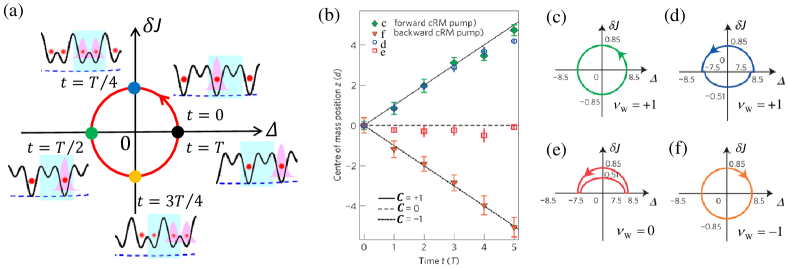
Figure 7: (Color online) Topological pumping in the Rice-Mele OL. (a) A pump cycle sketched in $\delta J$-$\Delta$ space with schematic of the pumping sequence. The pink shaded packet indicates the wave function of a particular atom initially localized at the unit cell. The wave function shifts to right as the pumping proceeds and moves the atom to the next unit cell after one pump cycle. (b) Results of four typical topological/trivial pumping (characterized by the Chern number $C=\pm 1,0$) with schematic pumping sequences in the $\delta J$-$\Delta$ plane shown in (c-f) and the winding number $\nu_{\text{w}}$ of each trajectory around the origin. (c) Charge pumped during a simple Rice-Mele pumping; (d) topologically nontrivial pumping; (e) topologically trivial pumping; and (f) negative sweep pumping. Reprinted by permission from Macmillan Publishers Ltd: Nakajima et al.[146], copyright© (2016).

Although topological charge pumping was first proposed more than thirty years ago, it has not yet been directly realized in condensed matter experiments. With ultracold atoms in tunable optical superlattices, the implementation of topological pumping has been extensively discussed [147, 148, 119, 149, 136, 150, 151, 152, 153, 154, 155]. In the context of the SSH/Rice-Mele model, it was theoretically demonstrated that the quantized particle pumping characterized by the non-zero Chern number can be realized in the cold atom systems [148, 119, 136], which is robust with respect to some perturbations in realistic experiments, such as nonzero temperature and the effects of finite sizes, non-adiabatic evolutions and trapping potentials. Moreover, as an extension of Thouless pumping, the topological pumping of interacting bosoinc and fermionic atoms trapped in OLs for specific models was also studied [147, 149, 151, 152, 153, 156]. For example, in the strongly interacting region, the bosonic atoms share the same transport properties as non-interacting fermions with quantized transport [147, 156]. Due to the degeneracy of the many-body ground states of the interacting bosons or fermions, the so-called topological fractional pumping (fractional values of the pumped particle) related to the many-body Chern number can be realized at certain fractional fillings [149, 151, 152, 153].

Recently, topological pumping has been realized in two experiments [146, 157] with ultracold fermionic and bosonic atoms in 1D optical superlattices, respectively. In the experiment in Ref. [146], an ultracold Fermi gas of ytterbium atoms ¹⁷¹Yb was loaded into a dynamically controlled optical superlattice, occupying the lowest energy band. The superlattice is formed by superimposing a long lattice $V_{L}$ and a short lattice $V_{S}$ with periodicity difference by a factor of two, and its time-dependent potential takes the form

$$V(x,t)=-V_{S}(t)\text{cos}^{2}\left(\frac{2\pi x}{d}\right)-V_{L}(t)\text{cos}^{2}\left(\frac{\pi x}{d}-\phi(t)\right),$$ (68)

where $\phi$ is the phase difference between the two lattices. By slowly sweeping $\phi$ over time, the lattice potential returns to its initial configuration whenever $\phi$ changes by $\pi$, thus completing a pumping cycle. The ability to tune all parameters of the lattice potential independently in a dynamic way offers the opportunity to realize various pumping protocols. In the absence of a static short lattice, $V(x,t)$ describes the simple sliding lattice that Thouless originally proposed [129]. In addition to this term, the double well lattice shown in Fig. 7 is realized, which can be described by the tight-binding Rice-Mele Hamiltonian in Eq. (62) for the alternating pumping. Figure 7 shows the schematics of the continuous pumping protocol as a closed trajectory in the $\delta J$-$\Delta$ parameter plane, where $\delta J\equiv(J-J^{\prime})/2$ is the modulation of the dimerization configurations. By sweeping the phase linearly in time $\phi(t)=\pi t/T$, one can periodically modulate the hopping amplitudes and on-site energies. In the experiment, topological pumping was detected as a shift of the center-of-mass of the atomic cloud measured with in situ imaging and the first Chern number $C$ of the pumping procedure was extracted from the average shift of the center-of-mass per pumping cycle, which is consistent with the ideal value $C=0,\pm 1$. The topological nature of the pumping was revealed by the pumping trajectories’ clear dependence on the topology in parameter space (denoted by the winding number $\nu_{\text{w}}$) as to whether or not a trajectory encloses the degenerate point. Pumping in the sliding lattice was demonstrated to be topologically equivalent to the continuous Rice-Mele pumping because of the same Chern numbers of the first band, which can be connected by a smooth crossover without closing the gap to the second band. It was also verified that the topological pumping indeed works in the quantum regime by varying the pumping speed and the temperature in the experiment [146].

In another experiment [157], the authors realized the topological pumping with ultracold bosonic atoms ⁸⁷Rb forming a Mott insulator in a similar dynamically controlled optical superlattice. Due to the large on-site interaction, each atom is localized on an individual double well, resulting in homogeneous delocalization over the entire first BZ. By taking in situ images of the atomic cloud in the lattice, they also observed a quantized deflection per pump cycle. The genuine quantum nature of the pumps was revealed by a counterintuitive reversed deflection of particles in the first excited band and a controlled topological transition in higher bands when tuning the superlattice parameters.

Also with bosonic atoms, a quantum geometric pump for a BEC in the lowest Bloch band of a tunable bipartite magnetic lattice was realized [158]. In contrast to the topological pumping yielding quantized pumping set by the global topological properties of the filled bands, the geometric pumping for a BEC occupying just a single crystal momentum state exhibits non-quantized particle pumping set by local geometrical properties of the band structure. For each pump cycle, a non-quantized overall displacement and a temporal modulation of the atomic wave packet’s position in each unit cell (i.e., the polarization) were observed [158].

These cold atom systems can be extended to implement more complex quantum pumping schemes, including spin degrees of freedom and in higher dimensions [159]. Analogous to Thouless pumping, topological pumping for spins without a net transport of charge may be constructed by imposing the TRS [160]. A spin pump with spin conservation can be composed of two independent pumps, where up and down spins have inverted Berry curvature and are transported in opposite directions. Spin pumps could serve as spin current sources for spintronic applications.

In a recent experiment [159], quantum spin pumping was implemented with ultracold bosonic atoms in two hyperfine states in a spin-dependent dynamically controlled optical superlattice, where each spin component is localized to a Mott insulator with negligible interspin interaction. In addition, the two spin components are coupled via spin-isotropic on-site interactions. For strong interactions $U\gg J$ (tunneling $J$ is suppressed) and unit filling, the system can be described by a 1D spin chain [159]:

$$\begin{aligned} H_{\text{SP}}=-\frac{1}{4}\sum_{n}\left[J_{\text{ex}}+(-1)^{n}\delta J_{\text{ex}}\right]\left({S}^{+}_{n}{S}^{-}_{n+1}+\text{h.c.}\right)+\frac{\Delta}{2}\sum_{n}(-1)^{n}{S}^{z}_{n}\end{aligned}$$ (69)

with spin-dependent tilt $\Delta$ and alternating exchange coupling $\frac{1}{2}\left(J_{\text{ex}}\pm\delta J_{\text{ex}}\right)$. For large tilts $\Delta\gg\frac{1}{2}\left(J_{\text{ex}}+\delta J_{\text{ex}}\right)$ the many-body ground state forms an antiferromagnetic ordered spins, while for strong exchange coupling $\frac{1}{2}\left(J_{\text{ex}}+\delta J_{\text{ex}}\right)\gg\Delta$ dimerized entangled pairs are favored. Varying $\delta J_{\text{ex}}$ and $\Delta$ during the pump cycle modulates ($\delta J_{\text{ex}},\Delta$) in the interacting 1D spin chain and encircles the degeneracy point, as shown in Fig. 8(a). After a full cycle, the two spin components move by a lattice site in opposite directions. This leads to a quantized spin transport described by the $\mathbb{Z}_{2}$ invariant as in the topologically equivalent case of independent spins [160]. Such a spin pump can be regarded as a dynamical version of the quantum spin Hall effect, where the parameter $\phi$ (the phase of the superlattice) is an additional dimension in a generalized 2D momentum space. The atomic spin current was measured and the net spin transport was further verified through in situ measurements of the spin-dependent center-of-mass displacement, as shown in Fig. 8(b).

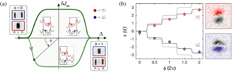
Figure 8: (Color online) Spin pumping in a spin chain of cold atoms. (a) A spin pump cycle in parameter space (green) of spin-dependent tilt $\Delta$ and exchange coupling dimerization $\delta J_{\text{ex}}$. The path can be parametrized by the angle $\phi$, acting as the pump parameter. The insets in the quadrants show the local mapping of globally tilted double wells to the corresponding local superlattice tilts with the black rectangles indicating the decoupled double wells. Between $\phi=0$ and $\pi$, $\left|\uparrow\right>$ and $\left|\downarrow\right>$ spins exchange their position, which can be observed by site-resolved band mapping images detecting the spin occupation on the left (L) and right (R) sites. (b) Center-of-mass position of up (red) and down (blue) spins as a function of $\phi$. Different absorption images of both sequences for $\left|\uparrow\right>$ and $\left|\downarrow\right>$ spins are shown on the right side. The solid lines depict the calculated motion of a localized spin for the ideal case (light gray) and for a reduced ground state occupation and a pump efficiency per half pump cycle that was determined independently through a band mapping sequence (gray). Reprinted with permission from Schweizer et al. [159]. Copyright© (2016) by the American Physical Society.

4.1.3 1D AIII class topological insulators

The topological or trivial character of a 1D insulator is completely determined by the presence or absence of chiral symmetry [123, 161, 61]. There are two distinct classes of 1D topological insulators, as chiral symmetry is the composition of time-reversal and charge-conjugation (particle-hole) symmetries. The first class is invariant under both the two symmetries and is called the BDI symmetry class represented by the SSH model. The second one is the AIII class with broken time-reversal and charge-conjugation symmetries, which still lacks experimental realization in condensed matter materials. The topology of the AIII class phase is quantified by an integer winding number. Recently, several works have been presented to study the 1D AIII class topological insulator using cold fermionic atoms in OLs [162, 163, 164, 165].

A simple dimerized lattice model for realizing the AIII class topological insulator was proposed in Ref. [163]. The Hamiltonian is given by

$$H_{\text{AIII}}=-\sum_{n}\left(Ja_{n}^{\dagger}b_{n}+J^{\prime}e^{i\theta}a_{n}^{\dagger}b_{n-1}+\text{h.c.}\right),$$ (70)

which is a generalization of the SSH model by introducing an acquired complex phase factor $e^{i\theta}$ ($\theta$ is a phase difference between the inter-cell and extra-cell hoppings) when particles tunnel from one unit cell to the next. It is worth noting that for open boundary conditions, the Hamiltonian $H_{\text{AIII}}$ in Eq. 70 is equivalent to $H_{\text{SSH}}$ in Eq. 59 through the gauge transformations, $(a^{\dagger}_{n},b_{n}^{\dagger})\rightarrow e^{-in\theta}(a^{\dagger}_{n},b_{n}^{\dagger})$. However, under the periodic boundary conditions, it is equivalent to the SSH model in a ring of $N$ lattice sites threaded by a magnetic flux $\phi=N\theta$. Therefore, under the periodic boundary conditions, this Hamiltonian still corresponds to the SSH model for $\theta=0$, while in the presence of this extra phase $\theta\neq 0,\pi$ (and $N\theta\neq 2m\pi$ with $m$ an integer), the model enters the AIII symmetry class. This model can be realized with spinless cold atoms by combining a 1D optical superlattice with the Raman assisted tunneling [163]. The Bloch Hamiltonian in this model is given by $\mathcal{H}_{\text{AIII}}(k)=-\left[J+J^{\prime}\text{cos}(k-\theta)\right]\sigma_{x}-J^{\prime}\text{sin}(k-\theta)\sigma_{y}$, which exhibits chiral symmetry for any value of $\theta$ since $\sigma_{z}\mathcal{H}_{\text{AIII}}(k)\sigma_{z}=-\mathcal{H}_{\text{AIII}}(k)$. For $\theta\neq 0,\pi$, it is not time reversal symmetric and thereby not charge-conjugation symmetric because $\mathcal{H}_{\text{AIII}}^{*}(-k)\neq\mathcal{H}_{\text{AIII}}(k)$ and no $2\times 2$ unitary transformation $U$ such that $U\mathcal{H}_{\text{AIII}}^{*}(-k)U^{\dagger}=\mathcal{H}_{\text{AIII}}(k)$ in this case.

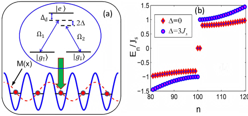
Figure 9: (Color online) Proposed optical Raman lattice for realizing the Hamiltonian (71). (a) Cold fermions trapped in 1D optical lattice with internal three-level $\Lambda$-type configuration coupled to radiation. (b) Energy spectra with open boundary condition in the topological ($\Delta=0$) and trivial ($\Delta=3J_{s}$) phases. The SO coupled hopping $J_{\rm so}=0.4J_{s}$. Reprinted with permission from Liu et al.[162]. Copyright© (2013) by the American Physical Society.

Another proposed model of 1D AIII class topological insulator is using spin-orbit-coupled fermionic atoms in an optical Raman lattice [162]. The atoms with the internal three-level $\Lambda$-type configuration are coupled through the transitions $|g_{\uparrow}\rangle,|g_{\downarrow}\rangle\rightarrow|e\rangle$ driven by the laser fields with Rabi-frequencies $\Omega_{1}(x)=\Omega_{0}\text{sin}(k_{0}x/2)$ and $\Omega_{2}(x)=\Omega_{0}\text{cos}(k_{0}x/2)$, as shown in Fig. 9(a). In the presence of a large one-photon detuning $|\Delta_{d}|\gg\Omega_{0}$ and a small two-photon detuning $2|\Delta|\ll\Omega_{0}$ for the transitions, the system Hamiltonian reads $H=H_{0}+H_{1}$, with $H_{0}=\sum_{\sigma=\uparrow,\downarrow}\bigr{[}\frac{p_{x}^{2}}{2m}+V_{\sigma}(x)\bigr{]}|g_{\sigma}\rangle\langle g_{\sigma}|+2\hbar\Delta|g_{\downarrow}\rangle\langle g_{\downarrow}|$, and $H_{1}=\hbar\Delta_{d}|e\rangle\langle e|-\hbar\bigr{(}\Omega_{1}|e\rangle\langle g_{\uparrow}|+\Omega_{2}|e\rangle\langle g_{\downarrow}|+{\rm H.c.}\bigr{)}$. Here the potentials $V_{\uparrow,\downarrow}(x)=-V_{0}\text{sin}^{2}(k_{0}x)$ form a 1D spin-independent OL. For $|\Delta_{d}|\gg\Omega_{0}$, the lasers $\Omega_{1,2}$ induce a two-photon Raman transition between $|g_{\uparrow}\rangle$ and $|g_{\downarrow}\rangle$. The effect of the small two-photon detuning is equivalent to a tunable Zeeman field along $z$ axis $\Gamma_{z}=\hbar\Delta$. Eliminating the excited state by $|e\rangle\approx\frac{1}{\Delta}(\Omega_{1}^{*}|g_{\uparrow}\rangle+\Omega_{2}^{*}|g_{\downarrow}\rangle)$ yields the effective Hamiltonian

$$H_{\rm eff} = \frac{p_{x}^{2}}{2m}+\sum_{\sigma=\uparrow,\downarrow}\bigr{[}V_{\sigma}(x)+\Gamma_{z}\sigma_{z}\bigr{]}|g_{\sigma}\rangle\langle g_{\sigma}|-\bigr{[}M(x)|g_{\uparrow}\rangle\langle g_{\downarrow}|+{\rm H.c.}\bigr{]},$$ (71)

where $M(x)=M_{0}\text{sin}(k_{0}x)$ with $M_{0}=\hbar\Omega_{0}^{2}/2\Delta_{d}$ represents a transverse Zeeman field induced by the Raman process. In the tight-binding regime, the system Hamiltonian can be recast into [162]

$$\tilde{H}_{\text{AIII}}=-J_{s}\sum_{<i,j>}(c_{i\uparrow}^{{\dagger}}c_{j\uparrow}-c_{i\downarrow}^{{\dagger}}c_{j\downarrow})+\sum_{j}\Gamma_{z}(n_{j\uparrow}-n_{j\downarrow})+\sum_{j}J_{{\rm so}}(c_{j\uparrow}^{\dagger}c_{j+1\downarrow}-c_{j\uparrow}^{\dagger}c_{j-1\downarrow})+{\rm H.c.}.$$ (72)

Here time reversal and charge conjugation operators are respectively defined by ${\hat{T}}=i\hat{K}\sigma_{y}$ with $\hat{K}$ being the complex conjugation, and ${\hat{C}}:(c_{\sigma},\ c^{\dagger}_{\sigma})\longmapsto(\sigma_{z})_{\sigma\sigma^{\prime}}(c^{\dagger}_{\sigma^{\prime}},c_{\sigma^{\prime}})$. The topological phase in this free-fermion system belongs to the chiral AIII class because while both ${\hat{T}}$ and ${\hat{C}}$ are broken in $\tilde{H}_{\text{AIII}}$, the chiral symmetry, defined as their product, is reserved since $({\hat{C}\hat{T}})\tilde{H}_{\text{AIII}}({\hat{C}\hat{T}})^{-1}=\tilde{H}_{\text{AIII}}$, with $({\hat{C}\hat{T}})^{2}=1$. In particular, this Hamiltonian describes a 1D topological insulator for $|\Gamma_{z}|<2J_{s}$ with two mid-gap zero edge modes and otherwise a trivial insulator, with the bulk gap $E_{g}=\mbox{min}\{|2J_{s}-|\Gamma_{z}||,2|J_{\rm so}|\}$, as shown in Fig. 9(b). It was shown that the zero edge modes in this 1D AIII topological insulator are spin polarized, with left and right edge spins polarized to opposite directions and forming a topological spin qubit of cold atoms [162]. A similar Raman lattice scheme was proposed to simulate symmetry-protected topological states using alkaline-earth-like atoms [164]. The interaction-driven topological phase transition for interacting fermionic atoms and a $\mathbb{Z}_{4}$ reduction of the 1D AIII class was also studied [162, 164].

A recent experiment [165] was reported to realize the 1D symmetry-protected topological state with cold fermionic atoms of ¹⁷³Yb in the optical Raman lattice. The experimental setup is similar as that proposed in Ref. [162], except that the potential forms a spin-dependent lattice with spin-dependent hopping strengths that explicitly break the locally defined chiral symmetry. In this case, the topological phase is protected by a magnetic group symmetry (defined as the product of time-reversal and mirror symmetries) and a nonlocal chiral symmetry. The topology of the cold atom system was measured via Bloch states at symmetric momenta and the spin dynamics after a quench between trivial and topological phases [165]. This work may open the way to explore the symmetry-protected topological states with ultracold atoms, including the chiral AIII class by considering spin-independent rather than spin-dependent OLs. Further generalization of this study to higher dimensional systems or interacting regimes also offers the simulation of quantum phases beyond natural conditions in solid-state materials.

4.1.4 Creutz ladder model

Initially introduced in the context of lattice gauge theory, the Creutz model [166] has gained a foothold in condensed matter physics as a versatile model to study fractionalization, Dirac fermions, and topological phases [167]. The model describes free fermions hopping on a two-leg ladder pierced by a $\pi$ magnetic flux. The Creutz ladder shown in Fig. 10(a) is described by the following Hamiltonian

$$H_{\text{CL}}=\frac{1}{2}\sum_{n}\big{[}\Omega c_{n}^{\dagger}\sigma_{x}c_{n}+c^{\dagger}_{n+1}(iJ_{0}\sigma_{z}-J_{1}\sigma_{x})c_{n}\big{]}+{\rm H.c.},$$ (73)

where $n$ is the site index containing up and down legs as the spin basis for the Pauli matrices, with the particle annihilation operators $c_{n}=(c_{nu},c_{nd})$. The fermions can jump from one site to the nearest-neighboring site within the same leg with a complex amplitude $\pm iJ_{0}$, i.e., gaining or losing a Peierls phase $\pi/2$. The fermions can hop between sites with amplitude $J_{1}$ while flipping between the legs, mimicking an SOC, and also horizontally along the legs with amplitude $\Omega$, mimicking a Zeeman field along $x$ axis. The corresponding Bloch Hamiltonian is given by $\mathcal{H}_{\text{CL}}(k)=J_{0}\text{sin}k\sigma_{z}+(w-J_{1}\text{cos}k)\sigma_{x}$. Consequently, there are two bands with the energy dispersion $E_{\pm}=\pm\sqrt{(J_{0}\text{sin}k)^{2}+(\Omega-J_{1}\text{cos}k)^{2}}$, as shown in Fig. 10(b). For periodic boundary conditions, the bands display a pair of massive Dirac fermions with different Wilson masses $m_{0}=J_{1}-\Omega$ at $k=0$ and $m_{\pi}=J_{1}+\Omega$ at $k=\pi$. When $J_{1}=\Omega$ ($J_{1}=-\Omega$), the system is gapless with a Dirac cone at momentum $k=0$ ($k=\pi$). When both $J_{1}$ and $\Omega$ vanish, the system exhibits two Dirac cones.

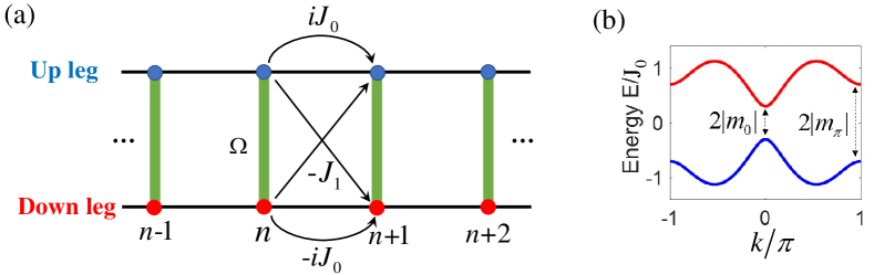
Figure 10: (Color online) (a) The Creutz ladder with up and down legs. Each lattice site encompasses a vertical bond with two leg states, containing an on-site coupling $\Omega$ and a leg-conserving hopping $\pm iJ_{0}$ and a leg-flip hopping $-J_{1}$, respectively. (b) Energy dispersion of the Creutz ladder model with gapped Dirac cones at $k=0$ and $\pi$ for $\Omega\neq\pm J_{1}$. The 1D Dirac points exhibit when $\Omega=\pm J_{1}$.

The Creutz ladder model is classified in the BDI class of topological insulators since the Hamiltonian has the particle-hole symmetry $\sigma_{z}\mathcal{H}_{\text{CL}}^{*}(k)\sigma_{z}=-\mathcal{H}_{\text{CL}}(-k)$, the TRS $\sigma_{x}\mathcal{H}_{\text{CL}}^{*}(k)\sigma_{x}=\mathcal{H}_{\text{CL}}(-k)$, and a chiral symmetry represented by $\sigma_{y}$ with $\{\mathcal{H}_{\text{CL}}(k),\sigma_{y}\}=0$. Therefore, the Creutz ladder is in the same symmetry class as the SSH model, exhibiting nontrivial band topology and edge states. In the SSH model, there are only two phases with different dimerization configurations. In the Creutz ladder model of fully gapped insulators, there are three phases distinguished by their bulk band topology as characterized by the Zak phase for all values of the parameters $(J_{1},\Omega)$: a trivial insulator with $\varphi_{Zak}=0$ when $|J_{1}/\Omega|<1$, two nontrivial insulators with $\varphi_{Zak}=\pi$ when $|J_{1}/\Omega|<1$ and $J_{1}>0$, and with $\varphi_{Zak}=-\pi$ when $|J_{1}/\Omega|<1$ and $J_{1}<0$. Equivalently, the band topology can be characterized by the winding number $\nu_{\text{w}}$ defined from the complex phase of the Bloch vectors: $\nu_{\text{w}}=\frac{1}{2}\big{[}\text{sgn}(\Omega+J_{1})-\text{sgn}(\Omega-J_{1})\big{]}$. In the topologically nontrivial phase there are two zero-energy bound states at the edges of the ladder with half fractional particle numbers.

Several recent works proposed schemes to realize and study the topological properties of the Creutz ladder model with cold atoms [168, 169, 170, 171, 172, 155, 173]. The general scheme of using cold atoms with artificial SOCs in a ladder-like OL under a synthetic magnetic field was suggested for simulation of the Creutz ladder [168]. The experimental setups capable of implementing the tunable Creutz ladder model were proposed in Refs. [170, 172, 155]. Several protocols that can be used to extract the topological properties in the Creutz model from atomic density and momentum distribution measurements as well as topological quantum pumping were presented [169, 170, 155]. By engineering a quantum walk with cold atoms, one can observe the topological phases and the bound states in the Creutz model [171]. By adding an energy imbalance between the two legs of the ladder, the symmetry class of the topological insulator changes from BDI to AIII [172]. Moreover, the interaction-induced topological phase transition in the presence of interatomic interactions in the optical Creutz ladder were investigated [170, 172]. A topological insulating phase protected by the inversion symmetry was found in a three-leg ladder model [173]. Notably, the realization of an optical two-leg ladder for ultracold bosonic atoms exposed to a uniform artificial magnetic field created by laser-assisted tunnelling has been experimentally achieved [174]. In the experiment, the atomic current on either leg of the ladder and the momentum distribution were observed for demonstrating chiral Meissner-like edge currents. Very recently, an experimental realization of a three-leg chiral ladder with ultracold fermionic atoms was reported [175], where the legs were formed by the orbital states of a 1D optical lattice and the complex inter-leg links were generated by the orbital-changing Raman transitions.

4.1.5 Aubry-André-Harper model

Recently, the topological properties of 1D quasiperiodic lattices have been theoretically and experimentally revealed in the context of cold atoms and photonic quasicrystals [176, 177]. The system exhibits topological edge states and nontrivial Chern numbers, equivalent to those of 2D quantum Hall systems on periodic lattices. The tight-binding Hamiltonian of the 1D quasiperiodic lattices takes the form:

$$H_{\text{AAH}}=-J\sum_{n}(c^{\dagger}_{n}c_{n+1}+\mathrm{H.c.})+\sum_{n}V_{n}c^{\dagger}_{n}c_{n},$$ (74)

where $V_{n}=V\text{cos}(2\pi\alpha n+\phi)$ is the spatially modulated on-site potential with $V$ being the strength, $\phi$ being the tunable modulation phase, and $\alpha$ controlling the periodicity of the modulation. When $\alpha$ is rational (irrational), the modulation is commensurate (incommensurate). Alternatively, the system Hamiltonian can be rewritten as

$$H_{\text{AAH}}\psi_{n}=-J(\psi_{n+1}+\psi_{n-1})+V\text{cos}(2\pi\alpha n+\phi)\psi_{n},$$ (75)

where $\psi_{n}$ is the wave function at site $n$. Historically, this model is known as the Aubry-André model [178] or Harper model [179].

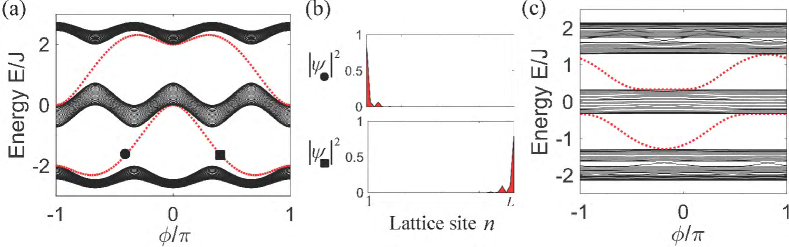
Figure 11: (Color online) Energy spectrum of the Aubry-André-Harper model as a function of the phase $\phi$ for (a) $\alpha=1/3$, $V=J=1$; and (b) $\alpha=(\sqrt{5}+1)/2$, $V=0.5$, $J=1$ under the open boundary condition in a lattice of site $L=98$. The density distribution of two typical in-gap edge states (red dotted lines) is depicted.

Figure 11 shows the energy spectrum of the Aubry-André-Harper model as a function of the modulation phase $\phi$ for a finite lattice of the length $L$ under the open boundary condition. In the commensurate potential ($\alpha=1/3$), the spectrum changes periodically as $\phi$ varies from $0$ to $2\pi$. The position of the edge states in the gaps also varies continuously with the change of $\phi$, which is localized either on the left or on the right boundary of the system. In the incommensurate potential ($\alpha=(\sqrt{5}+1)/2$), the spectrum is broken into a fractal set of bands; however, the in-gap edge states also exhibit and sweep across the gaps.

Due to the bulk-edge correspondence, the in-gap edge states are generally associated with the topologically nontrivial bulk bands. It was revealed that the topological properties in the 1D quasiperiodic lattices are assigned nontrivial Chern numbers in a 2D quantum Hall system [176, 177]. Specifically, the Aubry-André-Harper model is connected to the Hofstadter model (see Sec. 4.2.2), which describes electrons hopping on a 2D square lattice in a perpendicular magnetic field, with the eigenvalue problem described by the Harper equation: $-J_{x}(\psi_{n-1}+\psi_{n+1})-2J_{y}\text{cos}(2\pi\alpha n-k_{y})\psi_{n}=E(k_{y})\psi_{n}$, where $J_{x}$ ($J_{y}$) is the hopping amplitude along the $x$ ($y$) direction. By substitutions of $J\rightarrow J_{x}$, $V\rightarrow-2J_{y}$, and $\phi\rightarrow-k_{y}$, the current 1D problem can be mapped to the lattice version of the 2D integer QHE problem. Adiabatically varying $\phi$ from $0$ to $2\pi$ for each Bloch band forms an effective 2D manifold of Hamiltonian $H(k,\phi)$ in the $k$-$\phi$ parameter space, where the first Chern number can be defined.

For cold atoms, the Aubry-André-Harper model has been experimentally realized in 1D optical superlattices for studying localization phenomena [73, 180]. In the experiments, the quasiperiodic lattices were created using a primary 1D OL $V_{1}$ and an additional weak lattice $V_{2}$, with the wave numbers $k_{1}$ and $k_{2}$, respectively. For deep potentials, the atomic system is governed by the tight-binding Hamiltonian $H=H_{1}+H_{2}$, with $H_{1}=-J\sum_{n}(c_{n+1}^{\dagger}c_{n}+c_{n-1}^{\dagger}c_{n})$ from the primary lattice, and $H_{\text{2}}=V_{2}\sum_{n}c^{\dagger}_{n}c_{n}\text{cos}(2\pi\alpha n+\phi)$ from the interference of the perturbation lattice, where $V_{2}\sim J\ll V_{1}$, $\alpha=k_{2}/k_{1}$, and $\phi$ is the tunable relative phase. It was suggested that the energy spectrum and the Chern numbers can be revealed by observing the density profile of trapped fermionic atoms [176], which display plateaus with their positions uniquely determined by varying the parameter $\alpha$ of the optical superlattices. Another method to create and study quasiperiodic OLs underlying all quasicrystals by the abstract cut-and-project construction was recently proposed [181].

It was shown that the commensurate off-diagonal Aubry-André-Harper model is topologically nontrivial in the gapless regime and supports zero-energy edge modes [182], which is attributed to the topological properties of the 1D Majorana chain of $\mathbb{Z}_{2}$ class. By generalizing the spinless Aubry-André-Harper model to a spinfull version, which can be realized with spin-1/2 atoms in a spin-dependent quasiperiodic OL, one can realize the $\mathbb{Z}_{2}$ topological insulators and the topological spin pumping [183]. The phases of ultracold spin-1/2 bosons with SOCs in the quasiperiodic optical lattice were also studied [184]. In the presence of the pairings or interactions, the topological superconducting phase with Majorana end modes [185, 186, 187], the fractional topological phases connecting to the 2D fractional QHE [188], and the topological Bose-Mott insulators [189] in the quasiperiodic lattices have been theoretically investigated.

4.2 Two-dimension

4.2.1 Graphene-like physics and Dirac fermions

The graphene material, formed with a single layer of carbon atoms arranged in a honeycomb lattice with its low-energy quasipaticles described by the massless Dirac equation [190], has recently attracted strong interest in condensed-matter physics. The crystal structure of graphene, as shown in Fig. 12(a), consists of sublattices A (solid) and B (open). Its energy spectrum is shown in Fig. 12 (b), where two inequivalent points denoted as $\mathbf{K}$ and $\mathbf{K}^{\prime}$ are Dirac points. At a Dirac point, two energy bands intersect linearly and the quasiparticles in the vicinity of these points are described by the Hamiltonian $H_{D}$ and are frequently called “Dirac fermions”, where $H_{D}$ is the Dirac Hamiltonian in two spatial dimensions given by

$$H_{D}=v_{x}\sigma_{x}p_{x}+v_{y}\sigma_{y}p_{y}+\Delta_{g}\sigma_{z}.$$ (76)

Here $\sigma_{x,y,z}$ are the three Pauli matrices. Compared with the standard energy-momentum relation for the relativistic Dirac particles, here $\Delta_{g}$ and $v_{x,y}$ denote rest energy and the effective velocity of light respectively. For $\Delta_{g}\neq 0$, the energy spectrum with a gap denotes the massive Dirac fermions , as shown in Fig. 12(b). In graphene, by contrast, the Dirac points appear at the corners ($\mathbf{K}$ and $\mathbf{K}^{\prime}$ points) where the dispersion relation of the honeycomb lattice shows the conical intersection between the first and second bands. Here, the low-energy fermionic excitations are the massless Dirac fermions described by the Dirac Hamiltonian (76) with $\Delta_{g}=0$, $v_{x}=\pm v_{y}=\pm v$. Moreover, the associated Berry phases of the Dirac points are $\pm\pi$ [190, 191, 140] where the corresponding Berry curvatures have the form

$$\Omega_{n}=\pm\pi\delta\big{(}\mathbf{k}-\mathbf{K}_{n}\big{)}.$$ (77)

Here $\mathbf{K}_{n}$ denotes the Dirac points $\mathbf{K}$ or $\mathbf{K}^{\prime}$. One can see that the Berry curvatures tend to infinity at Dirac points. Here the Dirac points with the quantization of Berry phase (to $0$ and $\pi$) require symmetry protection, which can be the composition of inversion and time reversal symmetries. This is in contrast to Weyl points in 3D (see Sec. 4.3.2), which do not require any symmetry protection at all.

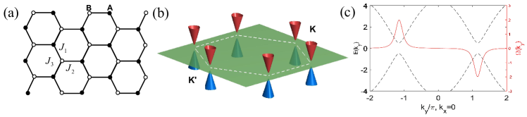
Figure 12: (Color online) (a) Crystal structure of a honeycomb lattice consisting of sublattices A (solid) and B (open). The nearest-neighbor hopping amplitudes denoted as $J_{1}$, $J_{2}$, $J_{3}$ corresponding to the three different directions. (b) Energy bands of the low-energy excitations with a gap. The first BZ is outlined by the dashed line, and two inequivalent valleys are labelled $\mathbf{K}$ and $\mathbf{K}^{\prime}$, respectively. Reprinted with permission from Xiao et al.[192]. Copyright© (2007) by the American Physical Society. (c) The energy spectrum (dashed) and Berry curvature (solid) of the conduction bands of a honeycomb lattice with broken inversion symmetry.

Since the relativistic Dirac fermions were found in graphene, a substantial amount of effort has been devoted to the understanding of exotic relativistic effects in solid-state systems and other artificial quantum systems [14, 23, 52]. Given these exciting results and the state-of-the-art technologies in quantum control of atoms, one topic that naturally arises is how to mimic the graphene and the relativistic quasiparticles with cold atoms in a similar 2D hexagonal lattice [76, 193, 194, 195, 196]. In cold atomic systems, it is easy to realize the anisotropy Hamiltonian with mass term $\Delta_{g}\neq 0$ and $v_{x}\neq v_{y}$ due to the highly controllable experimental parameters [76]. Furthermore, the detection of the Berry curvature can spread over a finite range, which provides a feasible way to measure the Berry phase over the first BZ in reciprocal space [140]. In addition to the honeycomb lattice, Dirac fermions can emerge in some lattices of other geometric structures [197, 198, 199, 200, 201, 202, 203, 204, 205].

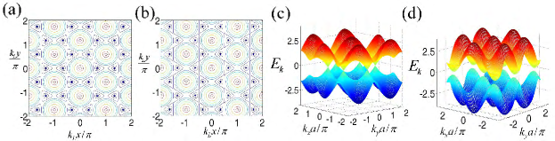
Figure 13: (Color online) The honeycomb optical lattices. (a),(b) The contours with three potentials described in Eq. (78). The minima of the potentials are denoted by the solid dots. All $V^{0}_{j}$ are the same in (a), and $V^{0}_{1}=V^{0}_{2}=0.91V^{0}_{3}$ in (b). The dispersion relations are shown in (c) for $\beta=1$ (gapless state) and (d) for $\beta=2.5$ (gapped state). Reprinted with permission from Zhu et al.[76]. Copyright© (2007) by the American Physical Society.

Simulating Dirac equations with cold atoms loaded in a honeycomb OL was initially proposed in Ref. [76]. In the proposal, single-component fermionic atoms (e.g., spin-polarized atoms ⁴⁰K, ⁶Li, etc.) trapped in a 2D ($x$-$y$ plane) hexagonal OL are considered. The hexagonal OL is constructed by three standing-wave laser beams with the corresponding potential

$$V(x,y)=\sum_{j=1,2,3}V_{j}^{0}\text{sin}^{2}\Big{[}k_{L}(x\text{cos}\theta_{j}+y\text{sin}\theta_{j})+\frac{\pi}{2}\Big{]},$$ (78)

where $\theta_{1}=\pi/3$, $\theta_{2}=2\pi/3$, $\theta_{3}=0$, and $k_{L}$ is the optical wave vector. It is easy to tune the potential barriers $V^{0}_{j}$ by varying the laser intensities along different directions to form a standard hexagonal lattice for $V^{0}_{1}=V^{0}_{2}=V^{0}_{3}$, or a hexagonal lattice with a finite anisotropy for different $V^{0}_{j}$ as depicted in Fig. 13(a) and 13(b), respectively. The tight-binding Hamiltonian of the system is then given by

$$H=-\sum_{\langle i,j\rangle}J_{ij}(a^{\dagger}_{i}b_{j}+{\rm H.c.}),$$ (79)

where $\langle i,j\rangle$ represents the neighboring sites, $a_{i}$ and $b_{j}$ denote the fermionic mode operators for the sublattices A and B, respectively. The tunneling amplitudes $J_{ij}$ depend on the tunneling directions in an anisotropic hexagonal lattice, denoted as $J_{1}$, $J_{2}$, and $J_{3}$ corresponding to the three different directions as illustrated in Fig. 12(a). For simplicity, assume $J_{1}=J_{2}=J$ and $J_{3}=\beta J$ with $\beta$ being the anisotropy parameter. As the atomic tunneling rate in an OL is exponentially sensitive to the potential barrier, this control provides an effective method to control the anisotropy of the atomic tunneling by laser intensities. The first BZ of this system also has a hexagonal shape in the momentum space with only two of the six corners in Fig. 12(b) being inequivalent, corresponding to two different sites $A$ and $B$ in each cell in the real hexagonal lattice, usually denoted as $\bf K$ and ${\bf K}^{\prime}$. One can choose ${\mathbf{K}}=(2\pi/a)(1/\sqrt{3},1)$ and ${\mathbf{K}^{\prime}}=-{\mathbf{K}}$, where $a=2\pi/(\sqrt{3}k_{L})$ is the lattice spacing. Taking a Fourier transform $a^{\dagger}_{i}=(1/\sqrt{N})\sum_{{\mathbf{k}}}{\rm exp}(i{\mathbf{k}}\cdot{\mathbf{A}}_{i})a_{\mathbf{k}}^{\dagger}$ and $b^{\dagger}_{j}=(1/\sqrt{N})\sum_{{\mathbf{k}}}{\rm exp}(i{\mathbf{k}}\cdot{\mathbf{B}}_{j})b_{\mathbf{k}}^{\dagger}$, where ${\mathbf{A}}_{i}$ (${\mathbf{B}}_{j}$) represents the position of the site in sublattice $A$ ($B$) and $N$ is the number of sites of the sublattice, the Hamiltonian (79) can be diagonalized with the expression of energy spectrum[76]

$$E_{\mathbf{k}}=\pm J\sqrt{2+\beta^{2}+2\text{cos}(k_{y}a)+4\beta\text{cos}(\sqrt{3}k_{x}a/2)\text{cos}(k_{y}a/2)}.$$ (80)

As plotted in Fig. 13(c) and 13(d), there are two branches of the dispersion relation, corresponding to the $\pm$ sign in Eq. (80). When $0<\beta<2$, the two branches touch with each other, and a Dirac cone structure appears around the touching points. It has the same standard Dirac cones as the graphene material with $\beta=1$ [190, 191, 206]. The Dirac cones squeeze in the $x$ or $y$ direction when $\beta$ deviates from $1$, but they still touch each other. When $\beta>2$, a finite energy gap $\Delta_{g}=|J|(\beta-2)$ appears between the two branches. So, across the point $\beta=2$, the topology of the Fermi surface changes, corresponding to a quantum phase transition without breaking any local symmetry [207]. Such a topological phase transition associated with the production or annihilation of a pair of Dirac points has been investigated in Ref.[208]. The evolution of the Dirac points in the hexagonal lattice by varying the asymmetric hopping and the resulting phase transition was also studied in Ref.[194]. With this phase transition, the system changes its behavior from a semimetal to an insulator at the half filling case (which means one atom per cell; note that each cell has two sites). Around half filling, the Fermi surface is close to the touching points, and one can expand the momentum ${\mathbf{k}}$ around one of the touching points ${\mathbf{K}}\equiv(k_{x}^{0},k_{y}^{0})$ as $(k_{x},k_{y})=(k_{x}^{0}+q_{x},k_{y}^{0}+q_{y})$. Up to the second order of $q_{x}$ and $q_{y}$, the energy spectrum (80) becomes

$$E_{\mathbf{q}}=\pm\sqrt{\Delta_{g}^{2}+v_{x}^{2}q_{x}^{2}+v_{y}^{2}q_{y}^{2}},$$ (81)

where $\Delta_{g}=0$, $v_{x}=\sqrt{3}\beta Ja/2$, and $v_{y}=Ja\sqrt{1-\beta^{2}/4}$ for $0<\beta<2$; $\Delta_{g}=|J|(\beta-2)$, $v_{x}=Ja\sqrt{3\beta/2}$, and $v_{y}=Ja\sqrt{\beta/2-1}$ for $\beta>2$. This simplified energy sprectrum $E_{\mathbf{q}}$ is actually a good approximation (named long wavelength approximation) as long as $q_{x}$, $q_{y}\lesssim 1/2a$. The wave function for the quasiparticles around half filling then satisfies the Dirac equation $i\hbar\partial_{t}\Psi=H_{D}\Psi$, where the relativistic Hamiltonian $H_{D}$ is the Dirac Hamiltonian with the form

$$H_{D}=\tau_{z}v_{x}\sigma_{x}q_{x}+v_{y}\sigma_{y}q_{y}+\Delta_{g}\sigma_{z},$$ (82)

where $\tau_{z}=\pm 1$ labels the two inequivalent valleys in Fig. 13(d). The corresponding Berry curvature is concentrated in the valleys and has opposite signs in the two inequivalent valleys. The symmetry property of the Berry curvature $\Omega(k)$: it is an odd function in the presence of TRS and even in the presence of inversion symmetry, as shown in Fig. 12(c). From Eq. (82), we can obtain the Berry curvature near the valleys for the conduction band[192]

$$\Omega(q)=\tau_{z}\frac{v_{x}v_{y}\Delta_{g}}{2(\Delta_{g}^{2}+v_{x}v_{y}q^{2})^{3/2}}.$$ (83)

Through an analogy to the graphene physics, one can realize both massive and massless Dirac fermions and observe the phase transition between them by controlling the lattice anisotropy [76]. This proposal was demonstrated to be experimentally feasible in Ref. [195], where the temperature requirement and critical imperfections in the laser configuration were considered in detail. Even in the presence of a harmonic confining potential, the Dirac points are found to survive [209]. In the presence of atomic interactions, the many-body physics of Dirac particles in graphene-type lattices, such as novel BCS-BEC crossover [210], topological phase transition between gapless and gapped superfluid [196] and even charge and bond ordered states with the $p$-orbital band of lattices [193, 211], have been investigated. Notably, a honeycomb lattice has been realized and investigated using a BEC [212, 213], but no signatures of Dirac points were observed. Even so, these important theoretical works pave the way for mimicking relativistic Dirac fermions and the aforementioned beyond-graphene physics with controllable systems.

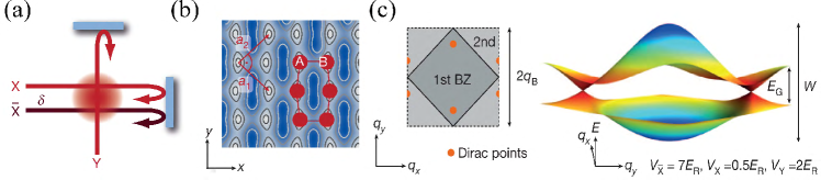
Figure 14: (Color online) Optical lattice with adjustable geometry. (a) Three retro-reflected laser beams create the 2D lattice potential of Eq.(84). (b) The real-space potential of the honeycomb lattice. (c) Left: sketch of the first and second BZs of the honeycomb lattice, indicating the positions of the Dirac points. Right: the energy spectrum of honeycomb lattice in the first BZ showing the linear intersection of the bands at the two Dirac points. The color scale illustrates lines of constant energy. $W$ and $E_{G}$ denote the full bandwidth and the minimum energy gap at the edges of the BZ, respectively; $q_{B}=2\pi/\lambda$ is the Bloch wavevector. Reprinted by permission from Macmillan Publishers Ltd: Tarruell et al.[77], copyright© (2012).

Subsequently, an experiment to realize Dirac points with adjustable properties using single-component ultracold fermionic atoms in a tunable honeycomb OL was reported in Ref. [77]. Furthermore, an artificial graphene consisting of a two-component ultracold atomic Fermi gas with tunable interactions was realized [214]. To create and manipulate Dirac points, the authors studied an ultracold Fermi gas of ⁴⁰K atoms in a 2D tunable OL [77]. In the experimental setup, three retro-reflected laser beams of wavelength $\lambda=1,064$nm are arranged to form the adjustable honeycomb OL, as shown in Fig. 14(a). The interference of two perpendicular beams $X$ and $Y$ can form a chequerboard lattice of spacing $\lambda/\sqrt{2}$. The third beam $\bar{X}$, collinear with $X$ but detuned by a frequency $\delta$, creates an additional standing wave with a spacing of $\lambda/2$. The yielding potential takes the form

$$V(x,y) =-V_{\bar{X}}\text{cos}^{2}(kx+\theta/2)-V_{X}\text{cos}^{2}(kx)$$ (84)

$$-V_{Y}\text{cos}^{2}(ky)-2\alpha\sqrt{V_{X}V_{Y}}\text{cos}(kx)\text{cos}(ky)\text{cos}(\varphi),$$

where $V_{\bar{X}}$, $V_{X}$ and $V_{Y}$ denote the single-beam lattice depths, $\alpha$ is the visibility of the interference pattern and $k=2\pi/\lambda$. Varying the relative intensities of the beams can realize various lattice structures, such as the chequerboard, triangle, square and honeycomb lattices. We focus on the honeycomb lattice with real-space potential as shown in Fig. 14(b). The primitive lattice vectors are perpendicular, leading to a square BZ with two Dirac points inside, as shown in Fig. 14(c). This lattice is called a brick-wall lattice, which is topologically equivalent to the honeycomb lattice.

The Dirac points here were characterized by probing the energy split between the two lowest-energy bands through inter-band transitions. They are topological defects in the band structure with the associated Berry phases $\pm\pi$, which guarantee their stability while a perturbation only moves the positions of Dirac points. However, breaking the inversion symmetry of the potential by introducing an energy offset $\Delta$ between the sublattices opens an energy gap at the Dirac points, as shown in the insets of Fig. 15(a). The band structure can be measured with the Bloch-Landau-Zener-oscillation technique [77, 215, 216] (see Sec. 5.1), and the results are plotted in Fig. 15(a), where the total fraction of atoms transferred to the second band $\xi$ is plotted as a function of the detuning $\delta$. The maximum indicates the point of inversion symmetry, where $\Delta=0$ and the gap at the Dirac point vanishes. Therefore, one can identify the points of maximum transfer with the Dirac points. To investigate how breaking the inversion symmetry of the lattice affects the Dirac points, the authors varied the sublattice offset $\Delta$, which is controlled by the frequency detuning $\delta$ between the lattice beams, and measured the total fraction of atoms transferred $\xi$. The population in the second band decreases symmetrically on both sides of the peak as the gap increases, indicating the transition from massless to massive Dirac fermions.

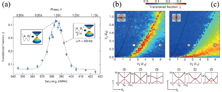
Figure 15: (Color online) Energy offset and topological transition. (a) The total fraction $\xi$ of atoms transferred to the second band as a function of the detuning $\delta$, which controls the sublattice energy offset $\Delta$. The maximum indicates the Dirac point. Insets: away from the peak, the atoms behave as Dirac fermions with a tunable mass. Solid line is a Gaussian fit to the data.The topological transition occurs along $q_{x}$ (b) and $q_{y}$ (c) directions in the quasi-momentum space. The dashed line is the theoretical result for the transition line, and the dotted line indicates the transition from the triangular lattice to the dimer lattice. The bottom diagrams show cuts of the band structure along the $q_{x}$ axis ($q_{y}$;(b)) and $q_{y}$ axis ($q_{x}$; (c)) for the values of $V_{X}$ and $V_{\bar{X}}$ indicated. Reprinted by permission from Macmillan Publishers Ltd: Tarruell et al.[77], copyright© (2012).

The position of the Dirac points inside the BZ and the slope of the associated linear dispersion relation are determined by the relative strength of the tunnel couplings (i.e., $J_{2}/J_{1},J_{3}/J_{1}$) [76, 194, 217], which can be adjusted simply by controlling the intensity of the laser beams. Therefore, it was observed that the positions of the Dirac points continuously approach the corners of the BZ when the tunnelling in the $x$ direction gradually increases by decreasing the intensity of $\bar{\text{X}}$. When they reach the corners of the BZ, the two Dirac points merge, annihilating each other. Beyond this critical point, a finite band gap appears for all quasimomenta of the BZ. This situation signals the transition between band structures of two different topologies, one containing two Dirac points and the other containing none. This corresponds to a Lifshitz phase transition from a semimetallic phase to a band-insulating phase in 2D honeycomb lattices at half-filling [76, 194]. The topological transition line was experimentally mapped out by recording the fraction of atoms transferred to the second band, $\xi$, as a function of the lattice depths $V_{\bar{\text{X}}}$ and $V_{X}$, while keeping the value of $V_{Y}/E_{R}$. The results are shown in Fig. 15(b). There the onset of population transfer to the second band signals the appearance of Dirac points in the band structure of the lattice. For a given value of $V_{X}$, the transferred fraction, $\xi$, decreases again for large values of $V_{\bar{\text{X}}}$, as the Dirac points lie beyond the momentum width of the cloud. The $\xi$ as a function of $q_{y}$ for a 1D lattice structure ($V_{\bar{\text{X}}}\gg V_{\text{X}}$) was obtained in Fig. 15(c), where the transition line is clearly demonstrated. This work opens the way to realize and investigate other topological models with cold atoms in OLs, such as the Haldane model [13] and Kane-Mele model [18, 19] to be addressed in Sec. 4.2.3 and 4.2.4, respectively.

After the realization of the Dirac points in the honeycomb OL using ultracold atoms, a further experiment to detect the $\pi$ Berry flux located at each Dirac point by realizing an atomic interferometer was reported [140]. The idea of detecting the Berry flux is analogous to using an Aharonov-Bohm interferometer to measure a magnetic flux in real space. As we know, the Aharonov-Bohm effect describes a charged particle wave packet being split into two parts that encircle a given area in real space [Fig. 16(a)]. Any magnetic flux through the enclosed area gives rise to a measurable phase difference between the two components. In analogy to the magnetic field, the Berry curvature $\Omega_{n}$ for a single Bloch band in the reciprocal space can be probed by forming an interferometer on a closed path in reciprocal space [Fig. 16(b)]. The geometric phase acquired along the path can be calculated from the Berry connection $\mathbf{A}_{n}(\mathbf{k})$, which is given by $\mathbf{A}_{n}(\mathbf{k})=\langle u^{n}_{\mathbf{k}}|i\nabla_{\mathbf{k}}|u^{n}_{\mathbf{k}}\rangle$. Here, $|u^{n}_{\mathbf{k}}(r)\rangle$ is the cell-periodic part of the Bloch wave function $|\psi^{n}_{\mathbf{k}}(\mathbf{r})\rangle=e^{i\mathbf{k}\cdot\mathbf{r}}|u^{n}_{\mathbf{k}}(r)\rangle$ with quasimomentum $\mathbf{k}$ in the $n$th band. Accordingly, the phase along a closed loop in reciprocal space is

$$\varphi_{\text{Berry}}=\oint_{\mathcal{L}}\mathbf{A}_{n}(\mathbf{k})d\mathbf{k}=\int_{S^{2}}\Omega_{n}(\mathbf{k})d^{2}\mathbf{k}.$$ (85)

where $S$ is the area enclosed by the path $\mathcal{L}=\partial_{S}$, and $\Omega_{n}(\mathbf{k})=\nabla\times\mathbf{A}_{n}(\mathbf{k})$.

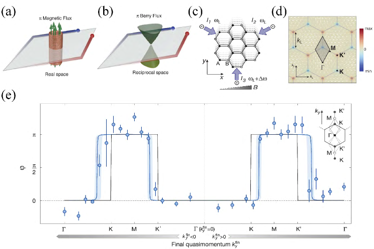
Figure 16: (Color online) Aharonov-Bohm analogy and geometric properties of the hexagonal lattice. (a) In the Aharonov-Bohm effect, electrons encircle a magnetic flux in real space. (b) In the interferometer, the particles encircle the $\pi$ Berry flux of a Dirac point in reciprocal space. (c) Sketch of the hexagonal lattice in real space, which is realized by interfering three laser beams (arrows) of intensity $I_{i}$ and frequency $w_{L}$, with linear out-of-plane polarizations. A linear frequency sweep of the third lattice beam creates a uniform lattice acceleration along the y direction. A magnetic field gradient along the $x$ axis creates an additional spin-dependent force. (d) Dirac points are located at the corners ($\mathbf{K}$ and $\mathbf{K}^{\prime}$ points) of the BZ (gray hexagons). Black diamond is a typical interferometer path. (e) Summary of phase shifts measured relative to the zero-area reference interferometer for different final quasimomenta $k_{y}^{fin}$ (Inset shows the interferometer paths). Lines follow ab initio theory using a full band structure calculation with no momentum spread $\sigma_{k}=0$ and perfectly localized Berry curvature $\delta k_{\Omega}=0$ (black) or $\sigma_{k}=0.21k_{L}$ and $\delta k_{\Omega}\simeq 10^{-4}k_{L}$ (blue). Reprinted from Duca et al.[140]. Reprinted with permission from AAAS.

In the experimental setup, the graphene-like hexagonal OL for ultracold ⁸⁷Rb atoms is implemented by superimposing three linearly polarized blue-detuned running waves at 120(1)^∘ angles (Fig. 16(c)). Fig. 16(d) shows that the resulting dispersion relation includes two inequivalent Dirac points with opposite Berry fluxes $\pm\pi$ located at $\mathbf{K}$ and $\mathbf{K}^{\prime}$, respectively. The interferometer sequence begins with an almost pure ⁸⁷Rb BEC in the state $|\uparrow\rangle=|F=2,m_{F}=1\rangle$ at quasimomentum $k=0$ in a $V_{0}=1$ $E_{r}$ deep lattice, where $E_{r}=h^{2}/(2m\lambda^{2}_{L})\approx h\times 4$ kHz is the recoil energy and $h$ is Planck’s constant. In fact, the method of detecting the Berry phase here is a 2D extension of the Zak phase’s measurement addressed in Sec. 4.1.1. The first step is to create a coherent superposition of $|\uparrow\rangle$ and $|\downarrow\rangle=|F=1,m_{F}=1\rangle$ states by using a resonant $\pi/2$-microwave pulse. Then a magnetic field gradient along $x$ axis is applied to create a constant force in opposite directions for the two spin components. Meanwhile, an orthogonal, spin-independent force from lattice acceleration is created by a linear frequency sweep of the third lattice beam and can move atoms along the $y$ direction [Fig. 16(c,d)]. As a consequence, the two spin components move symmetrically along the interferometer path in reciprocal space. After an evolution time $\tau$, a spin-echo $\pi$-microwave pulse is applied to swap the states $|\uparrow\rangle$ and $\downarrow\rangle$. Subsequently, the two atomic wave packets experience opposite magnetic forces in the $x$ direction, such that both spin components arrive at the same quasimomentum $k^{fin}$ after an additional evolution time $\tau$. At this point, the coherent superposition state is given by $|\psi^{fin}\rangle\propto|\uparrow,k^{fin}\rangle+e^{i\varphi}|\downarrow,k^{fin}\rangle$ with relative phase $\varphi$. Finally, a second $\pi/2$-pulse with a variable phase $\varphi_{MW}$ is applied in order to close the interferometer and convert the phase information into spin population fractions $n_{\uparrow,\downarrow}\propto 1\pm\text{cos}(\varphi+\varphi_{MW})$. Notably, the phase difference $\varphi=\varphi_{B}+\varphi_{d}$ consists of the geometric phase $\varphi_{B}$ and any difference in dynamical phases $\varphi_{d}$ between the two paths of the interferometer and is equal to the Berry phase of the region enclosed by the interferometer. This is because the dynamical contribution should vanish due to the symmetry of the paths and the use of the spin-echo sequence. To ascertain that the measured phase is truly of geometric origin, the authors additionally employed a zero-area reference interferometer, which comprises a V-shaped path produced by reversing the lattice acceleration after the $\pi$-microwave pulse.

The experimental results for detecting the Berry phase (flux) of the varying region enclosed by the interferometer are shown in Fig. 16(e). The results show that a phase difference $\varphi\simeq\pi$ when a Dirac point is enclosed in the measurement loop, which agrees well with the theoretical prediction of the Berry phase for a single Dirac point. In contrast, the phase difference vanishes when enclosing zero or two Dirac points. The shift in the phase jump results from the momentum spread $\sigma_{k}$, the broadening of the edges is caused by $\delta k_{\Omega}$, and the shaded area accounts for a variation in $\sigma_{k}=0.14-0.28k_{L}$. The contrast is limited by inhomogeneous broadening of the microwave transition, the finite momentum spread of the condensate, and, for large final quasimomenta, the dynamical instability of the Gross-Pitaevskii equation.

4.2.2 Hofstadter model

The celebrated Hofstadter model (also named as the Hofstadter-Harper model) describes charged particles moving in a 2D periodic lattice under a uniform magnetic flux per unit cell [218]. In the tight-binding regime, the single-particle energy spectrum depends sensitively on the number of flux quanta per unit cell and a band splits into narrow magnetic bands. At high magnetic fields, the self-similar energy spectrum was predicted to emerge, known as the Hofstadter butterfly. Moreover, for filled bands of non-interacting fermions when the Fermi energy lies in one of the band gaps, the Hall conductance of the system is quantized [10]. In this case, the Hofstadter model realizes the paradigmatic example of a topological insulator that breaks TRS and can be characterized by the first Chern numbers.

Consider the non-interacting spinless particles moving in a 2D square lattice in the presence of an artificial magnetic field, which are described by the Hofstadter Hamiltonian [218]

$$H_{H}=-J\sum_{m,n}\big{(}a^{\dagger}_{m+1,n}a_{m,n}+e^{i\varphi_{m,n}}a^{\dagger}_{m,n+1}a_{m,n}+\mathrm{h.c.}\big{)},$$ (86)

where $a^{\dagger}_{m,n}$ ($a_{m,n}$) is the creation (annihilation) operator of a particle at lattice site $(m,n)$, and $\varphi_{m,n}$ denotes the spatially-varying hopping phase induced by a magnetic flux $2\pi\phi$. Taking the Landau gauge, the Hofstadter Hamiltonian can be rewritten as

$$H_{H}=-J\sum_{m,n}\left(a^{\dagger}_{m+1,n}a_{m,n}+\mathrm{e}^{i2\pi m\phi}a^{\dagger}_{m,n+1}a_{m,n}+\mathrm{h.c.}\right).$$ (87)

With $y=na$ as the periodic coordinates on the system, this Hamiltonian can be diagonalized as a block Hamiltonian $H_{H}=\bigoplus{H}_{x}(k_{y})$, where $k_{y}$ is the quasimomenta along the periodic directions. The decoupled block Hamiltonian takes the form

$${H}_{x}(k_{y})=-J\sum_{m}(a^{\dagger}_{m+1}a_{m}+\text{h.c.})-\sum_{m}V_{m}a^{\dagger}_{m}a_{m},$$ (88)

where $V_{m}=2J\text{cos}(2\pi\phi m+k_{y}a)$. The single-particle wave function is written as $\Psi_{mn}=e^{ik_{y}y}\psi_{m}$, and then the Schrödinger equation $H_{x}(k_{y})\Psi_{mn}=E\Psi_{mn}$ reduces to the Harper equation [179]

$$-J(\psi_{m-1}+\psi_{m+1})-V_{m}\psi_{m}=E\psi_{m}.$$ (89)

For rational fluxes $\phi=p/q$ with $p$ and $q$ being relatively prime integers, and under the periodic boundary condition along $x$ axis, the wave function $\psi_{m}$ satisfies $\psi_{m}=e^{ik_{x}x}u_{m}(\mathbf{k})$ with $u_{m}(\mathbf{k})=u_{m+q}(\mathbf{k})$. In this case, the spectrum of this system consists of $q$ energy bands and each band has a reduced (magnetic) BZ: $-\pi/qa\leq k_{x}\leq\pi/qa$, $-\pi/a\leq k_{y}\leq\pi/a$. In term of the reduced Bloch wave function $u_{m}(\mathbf{k})$, Eq. (89) becomes

$$-J(e^{ik_{x}}u_{m-1}+e^{-ik_{x}}u_{m+1})-V_{m}u_{m}=E(\mathbf{k})u_{m}.$$ (90)

Since $u_{m}(\mathbf{k})=u_{m+q}(\mathbf{k})$, the problem of solving the equation (90) reduces to solving the eigenvalue equation, $M\Upsilon=E\Upsilon$, where $\Upsilon=(u_{1},...,u_{q})$ is the Bloch wave function for the $q$ bands and $M$ is the $q\times q$ matrix. The Hofstadter energy spectrum is displayed in Fig. 17, where the band gaps form continuous regions in the $\phi-E$ plane. When the Fermi energy lies in a gap, the system is an insulator, and the topological nature and the Hall conductance of the insulator do not change as long as the Fermi level remains within the same gap [10]. When the Fermi energy is in the gap between two bands $N$ and $N+1$, the quantized Hall conductance is $\sigma_{xy}=Ce^{2}/h$ with the topological Chern number

$$C=\frac{1}{2\pi}\sum_{n\leqslant N}\int_{-\pi/qa}^{\pi/qa}dk_{x}\int_{-\pi/a}^{\pi/a}dk_{y}F_{xy}^{(n)}(\textbf{k}),$$ (91)

where $F_{xy}^{(n)}$ is the Berry curvature of the $n$-th subband. As marked in Fig. 17, the largest two gaps correspond to topological insulators with the Chern number $C=\pm 1$, and the second largest ones have $C=\pm 2$.

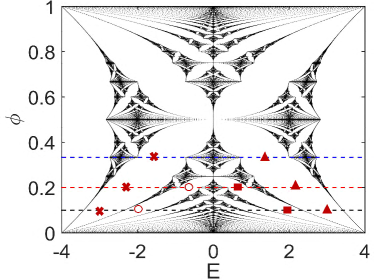
Figure 17: (Color online) Hofstadter-butterfly energy spectrum. Dashed lines represent the Fermi energy for different values of $\phi$, namely $\phi=1/3$, $1/5$, and $1/10$. Regions marked by $\times$ and $\blacktriangle$ have the band Chern numbers $C=\pm 1$; those marked by $\circ$ and $\blacksquare$ have $C=\pm 2$.

Despite its mathematical elegance, the Hofstadter butterfly and the topological Hofstadter insulator can hardly be realized in traditional solid-state systems because the magnetic field needs to be thousands of Tesla for electrons in order to create a magnetic flux comparable to one flux quantum per unit cell. However, some quantum Hall features associated with the fractal Hofstadter spectrum for low-energy Dirac fermions were recently observed in graphene superlattices and van der Waals heterostructures. [219, 220].

Recent theoretical and experimental advances in the creation of synthetic gauge fields for neutral atoms provide an excellent platform to simulate the physics of charged particles in magnetic fields. The concept of coupling two or several internal states to realize artificial magnetic fields was suggested in 2D OLs [114, 221, 222], which can be used to realize the Hofstadter model. In the proposals, the crucial element is the laser-assisted hopping between neighboring sites by Raman transitions. Because of the spatial variation of the Raman coupling, the wave function of an atom tunneling from one lattice site to another acquires an effective spatially-varying Berry phase. This method can also create non-Abelian U(2) gauge potentials acting on cold atoms in the OLs, leading to generalized Hofstadter butterfly spectra with new fractal structures and topological properties [222, 223].

The laser-assisted hopping scheme was further proposed by using a long-lived metastable excited state for alkaline-earth or ytterbium atoms in an optical superlattice to produce uniform magnetic fields for realizing the Hofstadter Hamiltonian [224]. It was also suggested to realize the uniform synthetic magnetic fields for neutral atoms by periodically shaking square OLs, and thus provided the Floquet realization of the Hofstadter Hamiltonian [225, 226, 121, 227, 228]. The atomic gas of noninteracting spinless fermions in a rotating OL was considered to study the Hofstadter butterfly and to measure the quantized Hall conductance of the Hofstadter insulator from density profiles using the Středa formula [229]. The evolution of the Hofstadter butterfly in a tunable OL among the square, checkerboard, and honeycomb structures was studied [230, 231]. A method for detecting topological Chern numbers in the Hofstadter bands by simply counting the number of local maxima in the momentum distribution from time-of-flight images of ultracold atoms was presented [232]. The detection of the fractal energy spectrum of the Hofstadter model from the density distributions of ultracold fermions in an external trap and under finite temperatures was analyzed [233]. The chiral edge states in the Hofstadter insulator may be created by using a steep confining potential in the OLs, and then they can be detected from the atomic Bragg spectroscopy and from their dynamics after the potential is suddenly removed [234, 235].

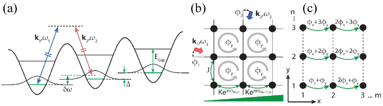
Figure 18: (Color online) (a) Raman-assisted tunneling in the lowest band of a tilted lattice with an energy offset $\Delta$ between neighboring sites. (b) Experimental geometry to generate uniform magnetic fields using a pair of far-detuned laser beams and a uniform potential energy gradient. (c) A schematic depicting the position-dependent phases of the tunneling process with resulting magnetic flux quanta per unit cell $\alpha=\phi_{y}/2\pi$. Reprinted with permission from Miyake et al.[29]. Copyright© (2013) by the American Physical Society.

Experimentally, the laser-assisted technique was used to generate large staggered magnetic fields for ultracold bosonic atoms [118], where the two internal states in the proposals [114, 224] were replaced by doubling the unit cell of the OL using superlattices. Two experiments were subsequently implemented for realizing the Hosftadter Hamiltonian based on the generation of homogeneous and tunable artificial magnetic fields with ultracold atoms in tilted OLs [29, 30]. In the experiments, the bosonic atoms were loaded in a square OL with a tilt potential along the $y$ direction, as shown in Fig. 18. The atomic tunneling in this direction was then suppressed by the linear tilt of energy per lattice site $\Delta\gg J$, which can be created with magnetic field gradients, gravity, or an ac Stark shift gradient. The tunneling is resonantly restored by the laser-assisted hopping method with two far-detuned Raman beams of two-photon Rabi frequency $\Omega$, frequency detuning $\delta\omega=\omega_{1}-\omega_{2}=\Delta/\hbar$, and momentum transfer $\delta\mathbf{k}=\mathbf{k_{1}}-\mathbf{k_{2}}\equiv(\delta k_{x},\delta k_{y})$, as shown in Fig. 18(a). Here the two Raman beams couple different sites, but do not change the internal state of the atoms, similar to the scheme proposed in Ref. [236]. In the dressed atom picture (for resonant tunneling along the $x$ axis) and high-frequency limit ($\delta\omega\gg J/\hbar$), the tilt disappears and time averaging over rapidly oscillating Raman beams yields an effective time-independent Hamiltonian for the lattice system, which takes the single-band form ($\Delta<E_{\text{Gap}}$) of the Hofstadter Hamiltonian:

$$\tilde{H}_{H}=-\sum_{m,n}\big{(}Ke^{-i\phi_{m,n}}a^{\dagger}_{m+1,n}a_{m,n}+Ja^{\dagger}_{m,n+1}a_{m,n}+h.c.\big{)}.$$ (92)

The induced hopping strength $K$ along the $x$ axis and the spatially-varying phase $\phi_{m,n}=\delta\mathbf{k}\cdot\mathbf{R}_{m,n}=m\phi_{x}+n\phi_{y}$ correspond to the vector potential $\mathbf{A}=\hbar(\delta k_{x}x+\delta k_{y}y)/a\>\hat{\mathbf{x}}$ instead of the simple Landau gauge. Adding up the accumulated phases around a closed path leads to an enclosed phase $\phi_{y}=\delta k_{y}a$ per lattice unit cell of area $a^{2}$, thus realizing the Hofstadter Hamiltonian with the magnetic flux $\alpha=\phi_{y}/2\pi$. When the frequencies of the Raman beams are similar to those used for the OL, one can tune the magnetic flux over the full range between zero and one by adjusting the angle between the Raman beams.

In the experiments, the laser-assisted tunneling processes was characterized by studying the expansion of the atoms in the lattice [29], and the local distribution of fluxes were determined through the observation of cyclotron orbits of the atoms on lattice plaquettes [30]. Since the laser-assisted hopping used does not require near-resonant light for connecting hyperfine states, this method can be implemented for any atoms, including fermionic atoms. Moreover, for two atomic spin states $|\uparrow,\downarrow\rangle$ with opposite magnetic moments and the titled potential created by a magnetic field gradient, two different spin components experience opposite directions of the magnetic field [30, 237], and the system naturally realizes the time reversal symmetric spinfull Hofstadter Hamiltonian:

$$H_{\uparrow,\downarrow}=-\sum_{m,n}\big{(}Ke^{\pm i\phi_{m,n}}a^{\dagger}_{m+1,n}a_{m,n}+Ja^{\dagger}_{m,n+1}a_{m,n}+h.c.\big{)},$$ (93)

which gives rise to the quantum spin Hall effect, topologically characterized by a $\mathbb{Z}_{2}$ spin Chern number. In a recent experiment [238], the weakly interacting ground state of the Hofstadter Hamiltonian (92) was studied, which for bosonic atoms is a superfluid BEC.

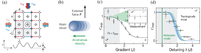
Figure 19: (Color online) Measurements of the Chern number of Hofstadter bands with ultracold bosonic atoms. (a) The setup consists of a 2D OL with a staggered potential. The magnetic unit cell (gray shaded area) is four times larger than the usual lattice unit cell. (b) The Chern number is extracted from the transverse displacement of the atomic cloud, in response to an external force generated by an optical gradient. Measured Chern number $C_{\mathrm{exp}}$ as a function of (c) gradient strength $Fa$; and (d) staggered detuning $\delta$. Reprinted by permission from Macmillan Publishers Ltd: Aidelsburger et al.[48], copyright © (2014).

The Chern numbers of the Hofstadter bands have been measured with ultracold bosonic atoms from the transverse deflection of an atomic cloud as a Hall response [48]. The experimental setup consisted of an ultracold gas of ⁸⁷Rb atoms loaded into a two-dimensional lattice created by two orthogonal standing waves with wavelength $\lambda_{s}=767\,\mathrm{nm}$. An additional standing wave with twice the wavelength $\lambda_{L}=2\lambda_{s}$ was superimposed along $x$ to create the staggered potential as shown in Fig. 19(a), with an energy offset $\Delta$ much larger than the bare tunneling $J_{x}$. The modulation restoring resonant tunneling was created by two additional pairs of far-detuned laser beams with wave number $k_{L}=2\pi/\lambda_{L}$ and frequency $\omega=\Delta/\hbar$. This system realized an effective time-independent Hofstadter Hamiltonian with the magnetic flux $\alpha=\pi/2$. In contrast to previous experiments generating uniform flux in tilted OLs [29, 30], this scheme does not rely on magnetic field gradients, providing a higher degree of experimental control. The incoherent distribution of bosonic atoms (where the population within each band is homogeneous in momentum space) was then loaded into the lowest Hofstadter band via an experimental sequence using an auxiliary superlattice potential, which introduces a staggered detuning $\delta$ along both directions [48]. For $\delta>2J$ the topology of the bands is trivial and all Chern numbers are zero. When crossing the topological phase transition at $\delta=2J$ (the spectral gaps close), the system enters the topologically non-trivial regime, where the lowest band has a Chern number $C=1$. The Chern numbers were finally extracted from the transverse Hall drift by exploiting Bloch oscillations. Under a constant force $\mathbf{F}=F\hat{\mathbf{e}}_{y}$, atoms on a lattice undergo Bloch oscillations along the $y$ direction. The cloud also experiences a net perpendicular (Hall) drift shown in Fig. 19(b) when the energy bands have a nonzero Berry curvature, which leads to an anomalous velocity that can be isolated by uniformly populating the bands. In the absence of inter-band transitions, the contribution of the $n$-th band to the center-of-mass motion along the $x$ direction can be written in terms of its band Chern number $C_{n}$ [48]:

$$x_{n}(t)=-\frac{4a^{2}F}{h}\,C_{n}\,t=-4a\,C_{n}\,\frac{t}{\tau_{B}},$$ (94)

where the factor $4a^{2}$ corresponds to the extended unit cell and $\tau_{B}=h/(Fa)$ is the characteristic time scale for Bloch oscillations. The center-of-mass evolution of the atomic cloud was measured in-situ with opposite directions of the flux $\alpha$ for subtracting the differential shift $x(t,\alpha)-x(t,-\alpha)=2x(t)$, as shown in Fig. 19(c), where the deflection is symmetric with respect to the direction of the applied force and gives an experimental Chern number $C_{\mathrm{exp}}\approx 1$. The measured drifts for $\alpha=0$ and for a staggered-flux distribution do not show any significant displacement, corresponding to zero Chern number. The dependence of the Chern-number measurement with respect to the force was studied, as shown in Fig. 19(d).

The chiral edge states of the Hofstadter lattice were experimentally observed in a ribbon geometry with an ultracold gas of neutral fermions [37] and bosons [38] subjected to an artificial gauge field and a synthetic dimension (see Sec. 4.4 for synthetic dimensions). Very recently, the following interacting Hofstadter model of bosons in the two-body limit was realized in OLs [239]:

$$H=-\sum_{i,j}\big{(}Ke^{-i\phi_{i,j}}a^{\dagger}_{i+1,j}a_{i,j}+Ja^{\dagger}_{i,j+1}a_{i,j}+h.c.\big{)}+\frac{U}{2}\sum_{i,j}n_{i,j}(n_{i,j}-1),$$ (95)

where $U$ is an on-site repulsive interaction energy. Through microscopic atomic control and detection [239], it was shown that the inter-particle interactions affect the populating of chiral bands, giving rise to chiral dynamics whose multi-particle correlations indicate both bound and free-particle characteristics. The novel form of interaction-induced chirality observed in these experiments provides the key piece for future investigations of highly entangled topological phases of many-body systems. The superfluid pairing and vortex lattices for interacting fermions in OLs under a uniform magnetic field was studied [240]. The Hofstadter-Hubbard model on a cylinder geometry with fermionic cold atoms in OLs was shown to allow one to probe the Hall response as a realization of Laughlin’s charge pump [241].

4.2.3 Haldane model

The well-known QHE in 2D electron systems is usually associated with the presence of a uniform externally generated magnetic field, which splits the electron energy spectrum into discrete Landau levels. In order to realize the integer QHE seen in the Landau-level problem while keeping the translational symmetry of the lattice, in 1988, Haldane proposed a spinless fermion model for the integer QHE without Landau levels[13]. He proposed that the QHE may result from the broken TRS without any net magnetic flux through the unit cell of a 2D hexagonal lattice, as illustrated in Fig. 20(a). The Haldane model based on breaking both time reversal and inversion symmetries is the first example of a topological Chern insulator, and the Hamiltonian is as follows

$$H=J_{1}\sum_{\langle{i,j}\rangle}c_{i}^{\dagger}{c_{j}}+J_{2}\sum_{\langle\langle{i,j}\rangle\rangle}e^{-iv_{ij}\phi}{c_{i}^{\dagger}{c_{j}}}+\sum_{i}{\epsilon_{i}c_{i}^{\dagger}{c_{i}}}.$$ (96)

Here the on-site energy $\epsilon_{i}$ is $\pm{M}$, depending on whether $i$ is on the $A$ or $B$ sublattice, $J_{1}$ is the nearest-neighbor-hopping energy, $J_{2}$ is the next-nearest-neighbor energy, and

$$v_{ij}=\text{sgn}(\hat{\mathbf{d}}_{i}\times\hat{\mathbf{d}}_{j})_{z}=\pm 1,$$ (97)

where $\hat{\mathbf{d}}_{i,j}$ are the unit vectors along the two bonds constituting the next-nearest neighbors the particle traverses going from site $j$ to $i$. As depicted in Fig. 20(a), a periodic magnetic flux density $\mathbf{B}(r)$ is added normal to the plane with the full symmetry of the lattice and with zero net flux through the unit cell. Thus, the flux $\phi_{a}$ and the flux $\phi_{b}$ in the regions $a$ and $b$ respectively has the relation $\phi_{b}=-\phi_{a}$: since the net flux is zero and the next-neighbor hoppings form closed loops in the hexagonal cell, the hopping terms $J_{1}$ are not affected but the hopping terms $J_{2}$ acquire a phase $\phi=2\pi(2\phi_{a}+\phi_{b})/\phi_{0}$ where $\phi_{0}$ is the flux quanta.

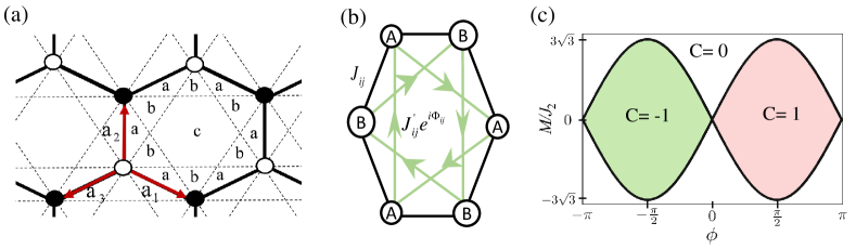
Figure 20: (Color online) (a) The Haldane honeycomb model showing nearest-neighbor bonds (solid lines) and next-nearest-neighbor bonds (dashed lines). The white and black dots represents the two sublattice sites $A$ and $B$ with different on-site energy $M$ and $-M$. The areas $a$ and $b$ are threaded by the magnetic flux $\phi_{a}$ and $\phi_{b}=-\phi_{a}$, respectively. The area $c$ has no flux. (b) A distorted honeycomb lattice realized in the experiment [28]. (c) Phases of the Haldane model.

Under the periodic condition, we can diagonalize the Haldane Hamiltonian by using the basis of a two-component spinor $c^{\dagger}_{k}=(c^{\dagger}_{k,A},c^{\dagger}_{k,B})$ of Bloch states constructed on the two sublattices. Let $\mathbf{a}_{1}$, $\mathbf{a}_{2}$, $\mathbf{a}_{3}$ be the displacements from a $B$ site to its three nearest-neighbor $A$ sites, as shown in Fig. 20(a), then $\mathbf{a}_{1}=(\frac{\sqrt{3}}{2}a,-\frac{1}{2}a),$ $\mathbf{a}_{2}=(0,a),$ $\mathbf{a}_{3}=(-\frac{\sqrt{3}}{2}a,-\frac{1}{2}a),$ where $a$ is the bond length. Taking a Fourier transform $c^{\dagger}_{i}=(1/\sqrt{N})\sum_{k}{e^{i\mathbf{k}\cdot\mathbf{r}_{i}}}c^{\dagger}_{k}$, where $\mathbf{r}_{i}$ represents the position of the site in sublattice $A$ or $B$ and $N$ is the number of sites of the sublattice, the Haldane Hamiltonian can be expressed as

$$\mathcal{H}(\mathbf{k})=\epsilon(\mathbf{k})+\mathbf{d}(\mathbf{k})\cdot\sigma,$$ (98)

where

$$\epsilon(\mathbf{k}) =2J_{2}\text{cos}{\phi}\sum^{3}_{i=1}{\text{cos}(\mathbf{k}\cdot\mathbf{b}_{i})},\leavevmode\nobreak\ \leavevmode\nobreak\ d_{1}(\mathbf{k})=J_{1}\sum^{3}_{i=1}\text{cos}(\mathbf{k}\cdot\mathbf{a}_{i}),$$ (99)

$$d_{2}(\mathbf{k}) =J_{1}\sum^{3}_{i=1}\text{sin}(\mathbf{k}\cdot\mathbf{a}_{i}),\leavevmode\nobreak\ d_{3}(\mathbf{k})=M-2J_{2}\text{sin}\phi\sum^{3}_{i=1}\text{sin}(\mathbf{k}\cdot\mathbf{b}_{i}),$$

with $\mathbf{b}_{1}=\mathbf{a}_{1}-\mathbf{a}_{2}$, $\mathbf{b}_{2}=\mathbf{a}_{3}-\mathbf{a}_{2}$, and $\mathbf{b}_{3}=\mathbf{a}_{1}-\mathbf{a}_{3}$. The BZ is a hexagon rotated $\frac{\pi}{2}$ with respect to the Wigner-Seitz unit cell: At its six corners $(\mathbf{k}\cdot\mathbf{a}_{1},\mathbf{k}\cdot\mathbf{a}_{2},\mathbf{k}\cdot\mathbf{a}_{3})$ is a permutation of $(0,\frac{2\pi}{3},-\frac{2\pi}{3})$. The two distinct corners $\mathbf{k}_{\alpha}^{0}$, are defined so that $\mathbf{k}_{\alpha}^{0}\cdot\mathbf{b}_{i}=\alpha\frac{2\pi}{3}$, $\alpha=\pm 1$. The energy spectrum of this system can be easily obtained by diagonalizing the Hamiltonian (98). There are two bands that touch only if all three Pauli matrix terms have vanishing coefficients, and only occur at the zone corner $\mathbf{k}_{\alpha}^{0}$ while $M=\alpha 3\sqrt{3}J_{2}\text{sin}{\phi}$.

To guarantee that the two bands never overlap and are separated by a finite gap unless they touch, in the following, we consider the case for $|J_{2}/J_{1}|<1/3$. One can choose the corner point $\mathbf{K}=\frac{2\pi}{3a}(1/\sqrt{3},1)$, then $(\mathbf{K}\cdot\mathbf{a}_{1},\mathbf{K}\cdot\mathbf{a}_{2},\mathbf{K}\cdot\mathbf{a}_{3})=(0,\frac{2\pi}{3},-\frac{2\pi}{3})$. We expand the Haldane Hamiltonian around the point $\mathbf{K}$ to linear order in $\mathbf{q}=\mathbf{k}-\mathbf{K}$:

$$\mathcal{H}_{+}=v(q_{x}\sigma_{x}-q_{y}\sigma_{y})+m_{+}\sigma_{z}$$ (100)

where $v=\frac{3}{2}J_{1}{a}$ and $m_{+}=M-3\sqrt{3}J_{2}\text{sin}{\phi}$. Hereafter, we ignore the $\mathbf{k}$-independent term $-3J_{2}\text{cos}{\phi}$, which plays no role in topology. At the other point $\mathbf{K}^{\prime}=-\frac{2\pi}{3a}(1/\sqrt{3},1)$, $(\mathbf{K}^{\prime}\cdot\mathbf{a}_{1},\mathbf{K}^{\prime}\cdot\mathbf{a}_{2},\mathbf{K}^{\prime}\cdot\mathbf{a}_{3})=(0,-\frac{2\pi}{3},\frac{2\pi}{3})$, around $\mathbf{K}^{\prime}$ we have

$$\mathcal{H}_{-}=v(-q_{x}\sigma_{x}-q_{y}\sigma_{y})+m_{-}\sigma_{z}$$ (101)

where $v=\frac{3}{2}J_{1}{a}$ and $m_{-}=M+3\sqrt{3}J_{2}\text{sin}{\phi}$. The Chern number of the whole system is determined by

$$C=\frac{1}{2}[\text{sgn}(m_{-})-\text{sgn}(m_{+})].$$ (102)

The phase diagram of the Haldane model as a function of $M/J_{2}$ and $\phi$ is shown in Fig. 20(c). For $\phi=0,\pi$, the model (98) is under time reversal, and the two mass $m_{+}$ and $m_{-}$ are equal, the system is trivial with $C=0$. Moreover, the system has the inversion symmetry when $M=0$. If $M$ and (or) $J_{2}\text{sin}{\phi}$ vanish, the two bands touch with gapless Dirac fermions. The model can have the nontrivial phases with $C=\pm 1$ only if $|M|<3\sqrt{3}J_{2}\text{sin}{\phi}$ and $\phi\neq 0,\pi$. Note that along the critical lines in the phase diagram where either $m_{+}$ or $m_{-}$ vanishes, the system experiences a topological phase transition, and has a low-lying massless spectrum around $\mathbf{K}$ or $\mathbf{K}^{\prime}$ simulating nondegenerate relativistic chiral Dirac fermions.

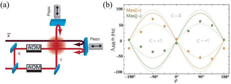
Figure 21: (Color online) (a) Laser beam set-up for forming the OL. The laser $\bar{X}$ is frequency-detuned from the other beams. Piezo-electric actuators sinusoidally modulate the retro-reflecting mirrors, with a controllable phase difference $\varphi$ that induces the complex tunneling phase $\Phi$. Acousto-optic modulators ensure the stability of the lattice geometry. (b) Topological phase diagram measured in the experiments. Solid lines show the theoretically computed topological transitions. Dotted lines represent the uncertainity of the maximum gap originating from the uncertainty of the lattice parameters. Data are the points of maximum transfer for each Dirac point. Reprinted by permission from Macmillan Publishers Ltd: Jotzu et al.[28], copyright© (2014).

Although the Haldane model has been proposed for nearly $30$ years, it has not been realized in any condensed matter systems since it is extremely hard to realize the required staggered magnetic flux assumed in the model. The technology of ultracold atoms in an OL provides an approach to realize and explore this model originally proposed in condensed matter physics. The idea of realizing and detecting the QHE of the Haldane model in an OL was first proposed in Ref. [242]. In the proposal, three standing-wave laser beams are used to construct a honeycomb OL where different on site energies in two sublattices required in the model can be implemented through tuning the phase of one laser beam. The other three standing-wave laser beams are used to create the staggered magnetic field. Firstly, to generate the honeycomb lattice with different on site energies in sublattices $A$ and $B$, the three laser beams with the same wave length but different polarizations are applied along three different directions: $\mathbf{e}_{y}$ and $\frac{\sqrt{3}}{2}\mathbf{e}_{x}\pm\frac{1}{2}\mathbf{e}_{y}$, respectively. Thus, the corresponding potential is given by

$$V=V_{0}[\text{sin}^{2}(\alpha_{+}+\frac{\pi}{2})+\text{sin}^{2}(yk^{L}_{0}+\frac{\pi}{3})\text{sin}^{2}(\alpha_{-}-\frac{\chi}{2})],$$ (103)

where $\alpha_{\pm}=\sqrt{3}xk^{L}_{0}/2\pm{yk^{L}_{0}/2}$, $V_{0}$ is the potential amplitude and $k^{L}_{0}$ is the wave vector of the laser. The ingenuity of the design is that the different site energies of sublattices $A$ and $B$ are controllable by the phase of the laser beam $\chi$. An interesting method to realize the staggered magnetic field in the Haldane model is to use two opposite-travelling standing-wave laser beams to induce Berry phase [84], which can create effective staggered magnetic fields with zero net flux per unit cell. For the two laser beams with Rabi frequencies $\Omega_{1}=\Omega_{0}\text{sin}(yk^{L}_{2}+\frac{\pi}{4})e^{ixk^{L}_{1}}$ and $\Omega_{2}=\Omega_{0}\text{sin}(yk^{L}_{2}+\frac{\pi}{4})e^{-ixk^{L}_{1}}$, the effective gauge potential is generated as $\mathbf{A}_{1}(\mathbf{r})=\hbar{k^{L}_{1}}\text{sin}(2yk^{L}_{2})\mathbf{e}_{x}.$ Here, $k^{L}_{1}=k^{L}\text{cos}\theta$ and $k^{L}_{2}=k^{L}\text{sin}\theta$ with $k^{L}$ being the wave vector of the laser and $\theta$ being the angle between the wave vector and the $\mathbf{e}_{x}$ axis. The choice of wave vector $k^{L}_{2}$ of the laser beams must be a multiple of $\frac{2\sqrt{3}\pi}{3a}$ in order to be commensurate with the OL, such as $k^{L}_{2}=\frac{2\sqrt{3}\pi}{3a}$. Since the lattice has the symmetry of point group $C_{3v}$, the other two vector potentials can be rotated by $\pm\frac{2\pi}{3}$ from the vector potential $\mathbf{A}_{1}$. Finally, the total accumulated phases along the nearest-neighbor directions are found to cancel each other out because of the symmetry of the honeycomb lattice. However, the total accumulated phases for the next-nearest-neighbor hopping are preserved as the hopping phase $\varphi=k^{L}_{1}a\text{sin}{\frac{ak^{L}_{2}}{\sqrt{3}}}$. Consequently, the total Hamiltonian of this cold atomic system is described by the Haldane model. However, in the proposal, the lasers for the honeycomb lattice and artificial magnetic fields are different and thus the required lasers are extremely complicated and hard to realize in practice.

Another scheme to realize the Haldane-like model was proposed in Ref. [243], with an orbital analogue of the anomalous QHE arising from orbital angular momentum polarization without Landau levels. This effect arises from the energy-level splitting between the on site $p_{x}-ip_{y}$ and $p_{x}+ip_{y}$ orbitals by rotating each OL site around its own center. At large rotation angular velocities, this model naturally reduces to two copies of Haldane’s quantum Hall model. An improved experimental proposal to realize the generalized Haldane model using OLs loaded with fermionic atoms in two internal states was proposed in Ref. [244]. In this simulation, the original phase factors in the next-nearest-neighbor hopping in Haldane’s paper are replaced by that in the nearest-neighbor, whose phase depends on the momentum imparted by the Raman lasers. An experimental scheme to realize the quantum anomalous Hall effect in an anisotropic square OL was proposed [203].

Instead of using the extra laser beams, one can create effective magnetic fields in the honeycomb OL by shaking the lattice [120, 28]. In $2014$, the first experimental realization of the Haldane model and the characterization of its topological band structure were reported [28], which used ultracold fermionic atoms in a periodically modulated honeycomb OL. In the experiment, the spin-polarized non-interacting ultracold Fermi gas of ⁴⁰K atoms was prepared in the OL created by several laser beams at wavelength $\lambda=1064$ nm. The lattice potential is given by

$$V(x,y,z)=-V_{\bar{X}}\text{cos}^{2}(k_{\text{lat}}x+\theta/2)-V_{X}\text{cos}^{2}(k_{\text{lat}}x)-V_{Y}\text{cos}^{2}(k_{\text{lat}}y)$$ (104)

$$-2\alpha\sqrt{V_{X}V_{Y}}\text{cos}(k_{\text{lat}}x)\text{cos}(k_{\text{lat}}y)\text{cos}(\varphi_{\text{lat}})-V_{\tilde{Z}}\text{cos}^{2}(k_{\text{lat}}z),$$

where $V_{\bar{X},X,Y,\tilde{Z}}$ are the single-beam lattice depths and $k_{\text{lat}}=2\pi/\lambda$. The energy offset $\Delta_{AB}$ can be controlled by varying $\theta$ around $\pi$ and changing the frequency detuning $\delta$ between the $\bar{X}$ and the $X$ (which has the same frequency as $Y$) beams using an acousto-optic modulator [77], as depicted in Fig. 21(a). $\varphi_{\text{lat}}$ is the relative phase of the two orthogonal retro-reflected beams $X$ and $Y$, the geometry of the lattice is actively stabilized at $\varphi_{\text{lat}}=0$, and the visibility of the interference pattern is $\alpha=0.81(1)$.

The crucial point for realizing the Haldane Hamiltonian in this experiment is the creation of the next-nearest neighbor tunneling, which is the complex tunneling with phase $\Phi_{ij}$. The complex tunneling $e^{i\Phi_{ij}}J^{\prime}_{ij}$ (see Fig. 20(b)) can be induced by circular modulation of the lattice position. The modulation applied in this experiment consists of moving the lattice along a periodic trajectory $\mathbf{r}_{\text{lat}}(t)$. Here, the time-dependence of the lattice position

$$\mathbf{r}_{\text{lat}}(t)=-A(\text{cos}[\omega{t})\mathbf{e}_{x}+\text{cos}(\omega{t}-\varphi)\mathbf{e}_{y}],$$ (105)

where $A$ is the amplitude of the motion, and $\omega/{2\pi}$ denotes the modulation frequency. Thus, after the atoms are loaded into the honeycomb lattice, a phase-modulated honeycomb lattice will be realized by ramping up the sinusoidal modulation of the lattice position $\mathbf{r}_{\text{lat}}$ along the $x$ and $y$ directions with a final amplitude of $0.087(1)\lambda$, frequency of $4.0$ kHz, and phase difference $\varphi$. This gives access to linear ($\varphi=0^{\circ}$ or $180^{\circ}$), circular ($\varphi=\pm 90^{\circ}$) and elliptical trajectories.

At this point, the effective Hamiltonian of this phase-modulated honeycomb lattice can be well described by the Haldane model, where the energy offset $\Delta_{AB}\gtrless{0}$ between sites of the $A$ and $B$ sublattices breaks inversion symmetry and opens a gap $|\Delta_{AB}|$. TRS can be broken by changing $\varphi$. This controls the imaginary part of the next-nearest-neighbor tunneling, whereas its real part, as well as the nearest-neighbor tunneling $J_{ij}$ and $\Delta_{AB}$, are mostly unaffected. To explore the topological properties of this system, the authors measured the band structure and probed the Berry curvature for the lowest band with different parameter $\Delta_{AB}$ and $\varphi$ by applying a constant force to the atoms, and it was found that orthogonal drifts are analogous to a Hall current. Meanwhile, one can map out the transition lines in the topological phase diagram of the Haldane model, as shown in Fig. 21(c), by identifying the vanishing gap at a single Dirac point.

4.2.4 Kane-Mele model

In $2005$, Kane and Mele [18, 19] generalized the Haldane model into the time reversal symmetric electron systems with spin. They introduced the spin-orbit interaction between electron spin and momentum to replace the periodic magnetic flux and predicted a new quantum phenomenon – the quantum spin Hall effect. Unlike the QHE where the magnetic field breaks TRS, the spin orbit interaction preserves TRS.

The Kane-Mele model takes the tight-binding Hamiltonian

$$H_{\text{KM}} = J\sum_{\langle{i,j}\rangle}c_{i}^{\dagger}{c_{j}}+i\lambda_{SO}\sum_{\langle\langle{i,j}\rangle\rangle}v_{ij}{c_{i}^{\dagger}{s_{z}}{c_{j}}}+i\lambda_{R}\sum_{\langle{i,j}\rangle}c_{i}^{\dagger}(\mathbf{s}\times{\mathbf{\hat{d}}_{ij}})_{z}{c_{j}}+\lambda_{v}\sum_{i}{\xi_{i}c_{i}^{\dagger}{c_{i}}}.$$ (106)

The first term is the usual nearest neighbor hopping term on a honeycomb lattice [Fig. 20(a)], where $c^{\dagger}_{i}=(c^{\dagger}_{i,\uparrow},c^{\dagger}_{i,\downarrow})$. The second term connecting next-nearest neighbors with a spin dependent amplitude is a mirror symmetric spin-orbit interaction. Here $v_{ij}=\pm 1$ is still the sign of hopping phases determined by the same form as Eq. (97). $s_{i}$ are the Pauli matrices describing the electron’s spin. The third term is a nearest neighbor Rashba term, which explicitly violates the $z\rightarrow{-z}$ mirror symmetry. The last term is a staggered sublattice potential with $\xi_{i}=\pm 1$ depending on whether $i$ is the $A$ or $B$ site, which will describe the transition between the quantum spin Hall phase and the simple insulator. If the Rashba term vanishes, the Kane-Mele model then reduces to independent copies for each spin of a Haldane model. In this case with $s_{z}$ being conserved, the distinction between graphene and a simple insulator is easily understood. Each spin has an independent Chern number $C_{\uparrow}$ and $C_{\downarrow}$. The TRS gives rise to $C_{\uparrow}+C_{\downarrow}=0$, but the difference $C_{\uparrow}-C_{\downarrow}$ is nonzero and defines a quantized spin Hall conductivity. This characterization breaks down when $s_{z}$ non-conserving terms are present ($\lambda_{R}\neq 0$), which makes the system more complicated. The electrons with spin-up and spin-down are coupled, and thus the spin Hall conductance is not quantized.

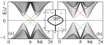
Figure 22: (Color online) Energy spectrum for a 1D zigzag strip in the (a) Quantum spin Hall phase $\lambda_{v}=0.1J$ and (b) the insulating phase $\lambda_{v}=0.4J$. In both cases $\lambda_{SO}=0.06J$ and $\lambda_{R}=0.05J$. The inset shows the phase diagram as a function of $\lambda_{v}$ and $\lambda_{R}$ for $0<\lambda_{SO}\ll{J}$. Reprinted with permission from Kane et al.[18]. Copyright© (2005) by the American Physical Society.

Following the method introduced in the Haldane model, we diagonalize the Hamiltonian by using a basis of the four-component spinor $c^{\dagger}_{k}=(c^{\dagger}_{k,A\uparrow},c^{\dagger}_{k,A\downarrow},c^{\dagger}_{k,B\uparrow},c^{\dagger}_{k,B\downarrow})$ of Bloch states constructed on the two sublattices and two spins. The generic $4\times{4}$ Hamiltonian can be written in the terms of Dirac matrices

$$\mathcal{H}_{\text{KM}}(\mathbf{k})=\sum^{5}_{a=1}d_{a}(\mathbf{k})\Gamma^{a}+\sum^{5}_{a<b=1}d_{ab}(\mathbf{k})\Gamma^{ab}.$$ (107)

Here, the five Dirac matrices are defined as

$$\Gamma^{a}=(\sigma_{x}\otimes{s_{0}},\sigma_{z}\otimes{s_{0}},\sigma_{y}\otimes{s_{x}},\sigma_{y}\otimes{s_{y}},\sigma_{y}\otimes{s_{z}})$$ (108)

(a=1,2,3,4,5); their $10$ commutators $\Gamma^{ab}=\frac{1}{2i}[\Gamma^{a},\Gamma^{b}]$, where the Pauli matrices $\sigma_{i}$ represent the sublattice indices; $\sigma_{0}$ and $s_{0}$ are the identity matrices. In this representation, the time reversal operator is given by $\hat{T}=i(\sigma_{0}\otimes{s_{y}})\hat{\mathcal{K}}$, where $\hat{\mathcal{K}}$ is the complex conjugation operator. The five Dirac matrices are even under the time reversal operator $\hat{T}$, $\hat{T}\Gamma^{a}\hat{T}^{-1}=\Gamma^{a}$, while the $10$ commutators are odd, $\hat{T}\Gamma^{ab}\hat{T}^{-1}=-\Gamma^{ab}$. To obtain a Hamiltonian preserving the TRS: $\hat{T}\mathcal{H}(\mathbf{k})\hat{T}^{-1}=\mathcal{H}(-\mathbf{k})$, the coefficients must satisfy the relations,

$$d_{a}(\mathbf{k})=d_{a}(-\mathbf{k}),\leavevmode\nobreak\ \leavevmode\nobreak\ d_{ab}(\mathbf{k})=-d_{ab}(\mathbf{-k}).$$ (109)

Therefore, the nonzero coefficients of Kane-Mele model are given by

$$d_{1}(\mathbf{k}) =J(1+2\text{cos}{x}\text{cos}{y}),d_{2}(\mathbf{k})=\lambda_{v},\leavevmode\nobreak\ \leavevmode\nobreak\ d_{3}(\mathbf{k})=\lambda_{R}(1-2\text{cos}{x}\text{cos}{y}),$$ (110)

$$d_{4}(\mathbf{k}) =-\sqrt{3}\lambda_{R}\text{sin}{x}\text{sin}{y},d_{12}(\mathbf{k})=-2J\text{cos}{x}\text{sin}{y},d_{15}(\mathbf{k})=2\lambda_{SO}(\text{sin}{2x}-2\text{sin}{x}\text{cos}{y}),$$

$$d_{23}(\mathbf{k}) =-\lambda_{R}\text{cos}{x}\text{sin}{y},\leavevmode\nobreak\ \leavevmode\nobreak\ \leavevmode\nobreak\ \leavevmode\nobreak\ d_{24}(\mathbf{k})=\sqrt{3}\lambda_{R}\text{sin}{x}\text{cos}{y},$$

with $x=\frac{\sqrt{3}}{2}k_{x}$, $y=-\frac{3}{2}k_{y}$, which are obtained through the variable transformations $\mathbf{k}\cdot\mathbf{b}_{1}=y+x$ and $\mathbf{k}\cdot\mathbf{b}_{2}=y-x$. Here $\mathbf{b}_{1}=(\frac{\sqrt{3}}{2}a,-\frac{3}{2}a)$ and $\mathbf{b}_{2}=(-\frac{\sqrt{3}}{2}a,-\frac{3}{2}a)$ are the lattice translation vectors in the honeycomb lattice shown in Fig. 20(a).

The four-band system becomes insulating when the lower two bands are fully occupied and an energy gap exists between the middle two bands. The phase diagram of the Kane-Mele model is shown in the inset of Fig. 22. For $\lambda_{R}=0$, the Hamiltonian reduces into two independent copies of Haldane Hamiltonian with different spins;we can define a spin-dependent Chern number $C_{s}$. For $\lambda_{v}>3\sqrt{3}\lambda_{SO}$, the gap is dominated by $\lambda_{v}$, and the system is a normal insulator since both Chern numbers $C_{\uparrow}$ and $C_{\downarrow}$ are zero. In contrast, for $\lambda_{v}<3\sqrt{3}\lambda_{SO}$, the corresponding Chern number becomes nonzero, $C_{\uparrow}=-C_{\downarrow}=\text{sgn}(\lambda_{SO})$. Although the total Chern number $C=C_{\uparrow}+C_{\downarrow}=0$, their difference $C_{\uparrow}-C_{\downarrow}=\pm 2$, which describes the quantum spin Hall phase with a pair of edge states crossing the bulk gap, as depicted in Fig. 22(a). For $\lambda_{R}\neq 0$, the $s_{z}$ symmetry is broken, and electrons with spin-up and spin-down mix together. Thus, we cannot introduce the spin-dependent Chern number to describe this system. Instead, Kane and Mele introduced the $\mathbb{Z}_{2}$ invariant (see Sec. A.3) to describe it.

Although the Kane-Mele model has been proposed for more than a decade, physicists still have not realized it or found such materials in condensed matter physics. To directly implement the Kane-Mele model is difficult, but the quantum spin Hall effect predicted by Kane and Mele was first experimentally realized in HgTe quantum wells [22]. Compared with conventional solid-state systems, cold atomic systems provide a perfectly clean platform with high controllability to construct and investigate the Kane-Mele-like model. There are several works in recent years proposing schemes to realize and study the topological properties of the quantum spin Hall insulators with cold atoms [245, 116, 246, 237]. An experimental scheme to simulate and detect the 2D quantum spin Hall insulator in a kagome OL was proposed in Ref. [245]. In this proposal, a kagome OL with the trimer and SOC terms can host the 2D quantum spin Hall insulator phase with only the nearest-neighbor hopping instead of the next-nearest-neighbor hopping in the Kane-Mele model. Moreover, the nearest-neighbor intrinsic SOC generated by the laser-induced-gauge-field method can be directly implemented in cold atomic experiments. Based on the investigation of the Hofstadter model on a 2D square OL [30, 29], one can construct the Kane-Mele-like model from two time-reversal copies of the spinless Hofstadter model [116, 246, 237]. Here, we briefly introduce a recent proposal on realizing time-reversal invariant topological insulators in alkali atomic gases [116], where quantum spin Hall states will emerge. In this model, particles with spin $\sigma=\uparrow,\downarrow$ experience a uniform magnetic flux per plaquette, but opposite in sign for the two spin components. The corresponding Hamiltonian is given by[116]

$$H=-J\sum_{m,n}c^{\dagger}_{m+1,n}e^{i\hat{\theta}_{x}}c_{m,n}+c^{\dagger}_{m,n+1}e^{i\hat{\theta}_{y}}c_{m,n}+\text{H.c.}+\lambda_{\text{s}}\sum_{m,n}(-1)^{m}c^{\dagger}_{m,n}c_{m,n},$$ (111)

where $c_{m,n}^{\dagger}$ is a two-component creation operator for fermonic atoms defined on a lattice site $(ma,na)$. The last term describes an on-site staggered potential with amplitude $\lambda_{\text{s}}$, along the $x$ direction, which has been introduced to drive transitions between different topological phases. The Peierls phases $\hat{\theta}_{x}=2\pi\gamma\sigma_{x}$ and $\hat{\theta}_{y}=2\pi m\Phi\sigma_{z}$ resulted from an artificial gauge field, are engineered within this tight-binding model to simulate the analog of SOCs. The effect of the $SU(2)$ link variable $\hat{U}_{y}(m)=e^{i\hat{\theta}_{y}}\propto\sigma_{z}$ is therefore analogous to the intrinsic SOC in Eq.(106). It corresponds to opposite magnetic fluxes $\pm\Phi$ for each spin component and generates quantum spin Hall phases. The link variable $\hat{U}_{x}=e^{i\hat{\theta}_{x}}\propto\text{sin}(2\pi\gamma)\sigma_{x}$ plays a role similar to the Rashba SOC in Eq. (106). For $\gamma=0$, this model corresponds to two decoupled copies of the spinless Hofstadter model. Besides, $\hat{\theta}_{x}$ mix the two spin components as they tunnel from one site to its nearest-neighbor sites. This model therefore captures the essential effects of the Kane-Mele model in a multi-band framework and offers the practical advantage of only involving nearest-neighbor hopping on a square lattice.

4.3 Three-dimension

4.3.1 3D Dirac fermions

As introduced in the previous sections, the 2D Dirac fermions have been extensively studied in graphene and honeycomb OLs. In recent years, it is of great interest to search for relativistic quasiparticles in 3D materials or artificial systems with stable band touching points, such as 3D Dirac(-like) fermions, which can exhibit transport properties different from those of 2D Dirac fermions. The Dirac equation in the Weyl representation is written as $i\hbar{\partial\Psi}/{\partial t}=H_{D}\Psi,$ where $\Psi$ denotes the four-component bispinor for 3D Dirac fermions and the Dirac Hamiltonian is given by

$$H_{D}=\left(\begin{array}[]{cc}v_{F}{\boldsymbol{\sigma}}\cdot{\mathbf{p}}&m\\ m&-v_{F}{\boldsymbol{\sigma}}\cdot{\mathbf{p}}\end{array}\right),$$ (114)

with the linear dispersion $E^{\pm}_{\rm D}=\pm\sqrt{v_{F}^{2}p^{2}+m^{2}}$. Here ${\boldsymbol{\sigma}}=(\sigma_{x},\sigma_{y},\sigma_{z})$ are Pauli matrices, ${\mathbf{p}}=(p_{x},p_{y},p_{z})$ is the 3D (quasi-)momentum, and the Fermi velocity $v_{F}$ and the mass term $m$ represent the effective speed of light and rest energy, respectively. Notably, the off-diagonal term $m$ in Eq. (114) mixes the two Weyl fermions (see the following section) of opposite chirality.

The Hamiltonian (114) can describe the transition between a 3D topological insulator and a trivial insulator in the critical case $m=0$. Recently, it was revealed that the Dirac points with fourfold degeneracies can be protected by certain symmetries [247, 248, 249] such as rotation or nonsymmorphic symmetries, which are not accidental band crossings at the transition between topological and trivial insulators. Thus, one has a topological Dirac semimetal with four band degeneracy, which can be viewed as 3D graphene, possessing 3D Dirac fermions in the bulk with linear dispersions along all momentum directions. These massless ($m=0$) 3D Dirac fermions have recently been observed in some compounds (for a comprehensive review of Dirac semimetals in 3D solids, see Ref. [24]).

Before the Dirac semimetals were discovered in materials, several schemes for simulating massless and massive 3D Dirac fermions with cold atoms in 3D OLs have been proposed [250, 251, 115, 168]. With cold fermions in an edge-centered cubic OL for proper parameters, the linear dispersion characterizing 3D Dirac-like particles with tunable mass can exhibit [250]. The system was proposed to realize 3D massless Dirac fermions in a cubic OL subjected to a synthetic frustrating magnetic field [251], and the mass term may be induced by coupling the ultracold atoms to Bragg pulses in the system. It was suggested that the massless and massive 3D relativistic fermions can also be simulated with ultracold fermionic atoms in 3D optical superlattices with Raman-assisted hopping [115, 168]. Moreover, by tuning the Raman laser intensities, the system may allow the decoupling of fermion doublers from a single Dirac fermion through inverting their effective mass [115], providing a quantum simulation of Wilson fermions [252].

4.3.2 Weyl semimetals and Weyl fermions

The Dirac equation (114) for massless particles can be rewritten in a simpler form:

$$i\hbar\frac{\partial\psi_{\pm}}{\partial t}=H_{W\pm}\psi_{\pm},\leavevmode\nobreak\ \leavevmode\nobreak\ H_{W\pm}=\pm v_{F}{\boldsymbol{\sigma}}\cdot{\mathbf{p}},$$ (115)

where $\psi_{\pm}$ are effectively two-component vectors acting as two chiral modes. This is the Weyl equation and $\psi_{\pm}$ are referred to as Weyl fermions, which propagate parallel (or antiparallel) to their spin and thus defines their chirality. There are no fundamental particles currently found to be massless Weyl fermions. In some 3D lattice systems, Weyl fermions can emerge as low-energy excitations near band crossings, and they always arise in pairs with opposite chirality and separated momenta. These systems are the so-called Weyl semimetals [253, 254, 255], which have been intensively investigated in the last couple of years. For more details, see the comprehensive review of vast theoretical and experimental studies of Weyl semimetals in 3D solids [24] and the references therein.

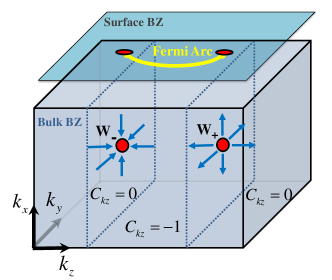
Figure 23: (Color online) A pair of Weyl points as the Berry flux monopole and anti-monopole in the bulk BZ. They are connected by surface Fermi arcs.

Let us use the following minimal two-band model for discussing the properties of Weyl semimetals in a simple cubic lattice. The Bloch Hamiltonian is given by

$$\mathcal{H}(\mathbf{k})=d_{x}(\mathbf{k})\sigma_{x}+d_{y}(\mathbf{k})\sigma_{y}+d_{z}(\mathbf{k})\sigma_{z}$$ (116)

with the Pauli matrices acting on two (pseudo-)spin states and the Bloch vectors

$$d_{x}=2J_{s}\text{sin}k_{x},\ \ d_{y}=2J_{s}\text{sin}k_{y},\ \ d_{z}=m_{z}-2J_{0}(\text{cos}k_{x}+\text{cos}k_{y}+\text{cos}k_{z}).$$ (117)

Here $J_{s}$ and $J_{0}$ denote the hopping amplitudes of spin-flipping hopping in the $xy$ plane and spin-dependent hopping along all the three dimensions, respectively, and $m_{z}$ represents the Zeeman field. For $2J_{0}<m_{z}<6J_{0}$, the bands $E_{\pm}(\mathbf{k})=\pm\sqrt{d_{x}^{2}+d_{y}^{2}+d_{z}^{2}}$ have two crossings in the first BZ located at $\mathbf{W}_{\pm}=(0,0,\pm\arccos k_{w})$ with $k_{w}=(m-4J_{0})/2J_{0}$. They are actually a pair of Weyl points (nodes) since one can obtain the effective Weyl Hamiltonian for low-energy excitations by approximating $H_{W\pm}(\mathbf{k})\approx\mathcal{H}(\mathbf{W}_{\pm}+\mathbf{q})$:

$$H_{W\pm}=v_{x}q_{x}\sigma_{y}+v_{y}q_{y}\sigma_{x}\pm v_{z}q_{z}\sigma_{z},$$ (118)

where $v_{x}=v_{y}=2J_{s}$ and $v_{z}=2J_{0}$. When the Fermi level is at $E_{F}=0$, the Fermi surface consists solely of two Weyl points and the system is the Weyl semimetal with emergent Weyl fermions. The Hamiltonian $H_{W\pm}$ can be written as $H_{\mathrm{W},\pm}=\sum_{i,j}q_{i}\alpha_{ij}\sigma_{j}$, where $[\alpha_{ij}]$ is a $3\times 3$ matrix with elements $\alpha_{xy}=\alpha_{yx}=2J_{s}$, $\alpha_{zz}=\pm 2J_{0}$ and zero otherwise. Thus the chirality of the two Weyl points $\mathbf{W}_{\pm}$ can be defined as $\chi_{\pm}=\mathrm{sgn}(\det[\alpha_{ij}])=\pm 1$, respectively. One can see that there is no matrix that anticommutes with $H_{W\pm}$ and opens a band gap since all three Pauli matrices are used up in $H_{W\pm}$. To further realize the topological stability of Weyl points, one can obtain the Berry flux

$$\mathbf{F}_{\pm}(\mathbf{k})=\pm\frac{\mathbf{k}}{2|\mathbf{k}|^{3}},$$ (119)

which is the source and sink of the Berry curvature, forming vector fields in momentum space that wraps around the Weyl points $\mathbf{W}_{\pm}$. As shown in Fig. 23, the pair of Weyl points act as the monopole and anti-monopole in the bulk BZ, which are characterized by the topological charges (Chern numbers)

$$C_{W\pm}=\frac{1}{2\pi}\oint_{S}\mathbf{F}_{\pm}(\mathbf{k})\cdot d\mathbf{S}=\pm 1=\chi_{\pm},$$ (120)

through any surface $S$ enclosing the points. This implies that the Weyl points always exhibit in pairs of opposite chirality, because the field lines of the Berry curvature must begin and end somewhere within the BZ. The only way to eliminate the Weyl points is to annihilate them pairwise by moving them at the same point in momentum space. Therefore, the stability of the Weyl points comes from their intrinsical topology. It is worth noting that unlike Dirac points, Weyl points necessitate the breaking of either (or both) time-reversal or space-inversion symmetry in lattice systems.

To further discuss the topological properties of Weyl semimetals, we consider the Bloch Hamiltonian (116,117) using the dimension reduction method. Treating $k_{z}$ as an effective parameter ($k_{z}$ being a good quantum number), we can reduce the original system to a ($k_{z}$-modified) collection of effective 2D subsystems described by $\mathcal{H}_{k_{z}}(k_{x},k_{y})$. If $k_{z}\neq\pm k_{c}$, the 2D bulk bands of $\mathcal{H}_{k_{z}}(k_{x},k_{y})$ are fully gapped and thus can be topologically characterized by the first Chern number

$$C_{k_{z}}=\frac{1}{4\pi}\int_{-\pi}^{\pi}dk_{x}\int_{-\pi}^{\pi}dk_{y}\leavevmode\nobreak\ \hat{d}\cdot\left(\partial_{k_{x}}\hat{d}\times\partial_{k_{y}}\hat{d}\right)=\left\{\begin{array}[]{ll}-1,\nobreak\leavevmode\nobreak\leavevmode&-k_{c}<k_{z}<k_{c};\\ 0,\nobreak\leavevmode\nobreak\leavevmode&|k_{z}|>k_{c},\end{array}\right.$$

where $\hat{d}\equiv\vec{d}/|\vec{d}|$. For any plane $-k_{c}<k_{z}<k_{c}$, one has $C_{k_{z}}=-1$ characterizing a Chern insulator, while elsewhere $C_{k_{z}}=0$ signals a trivial insulator. The value of $C_{k_{z}}$ changes for a topological phase transition only when the bulk gap closes at $\mathbf{W}_{\pm}=(0,0,\pm k_{c})$. From this point of view, the two Weyl points appear to be the critical points for the topological phase transitions. An important consequence is that the Fermi arc surface states arise in Weyl semimetals and terminate at the pair of Weyl points. When each of the 2D Hamiltonians $\mathcal{H}_{k_{z}}(k_{x},k_{y})$ represents a 2D Chern insulator, if one considers a surface perpendicular to the $x$ direction (still labeled by $k_{y}$ and $k_{z}$), each of the 2D Chern insulators will have a gapless chiral edge mode near the Fermi energy $E_{F}=0$. The Fermi energy will cross these states at $k_{y}=0$ for all $-k_{c}<k_{z}<k_{c}$, which leads to a Fermi arc that ends at the Weyl point projections on the surface BZ ($k_{y}$-$k_{z}$ plane), as shown in Fig. 23. In this particular model, the Fermi arc is a straight line. The Weyl fermions near the Weyl points and the Fermi arcs in a Weyl semimetals are fundamentally interesting and can give rise to exotic phenomena absent in fully gapped topological phases, such as anomalous (topological) electromagnetic responses [253, 254, 255, 24].

To realize this model of Weyl semimetals, a scheme has been proposed by using ultracold fermionic atoms in a 2D square OL subjected to experimentally realizable SOC and an artificial dimension from an external parameter space (acting as $k_{z}$) [136]. It was further shown that in the cold atom system, the simulated Weyl points can be experimentally detected by measuring the atomic transfer fractions in a Bloch-Landau-Zener oscillation, and the topological invariants of the Weyl semimetals can be measured with the particle pumping approach [136]. Another proposal to construct a Weyl semimetal was to stack 1D topological phases in double-well OLs with two artificial dimensions [256]. Similar 3D lattice models for realizing Weyl semimetals with cold atoms from stacking 2D layers of Chern insulators in checkerboard or honeycomb OLs with synthetic staggered fluxes were suggested in Refs. [257, 258, 259, 260]. The realization of chiral anomaly by using a magnetic-field gradient in the system was also discussed [258]. In these schemes, the spin degree of freedom can be encoded by two atomic internal states or sublattices, and then the required hopping terms can be realized by synthetic SOC or magnetic fields. These ingredients are well within current experimental reach of ultracold gases. It was illustrated that Weyl excitations can also emerge in 3D OL of Rydberg-dressed atomic fermions or dipolar particles [261, 262]. The Weyl points may automatically arise in the Floquet band structure during the shaking of a 3D face-centered-cubic OL without requiring sophisticated design of the tunneling [263].

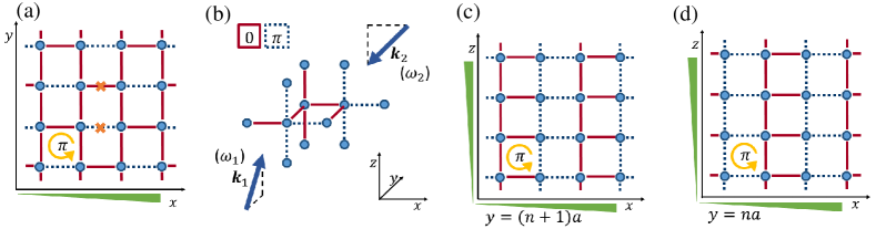
Figure 24: (Color online) Sketch of the 3D cubic lattice with engineered hopping along $x$ and $z$ directions, which possesses Weyl points in momentum space. Dashed and solid lines depict hopping with acquired phase $\pi$ and $0$, respectively. (a) The $xy$ planes of the lattice are equivalent to the lattice of the Hofstadter-Harper Hamiltonian with $\alpha=1/2$ flux. Green triangles along the axes denote the tilted directions. (b) A pair of Raman lasers enabling laser-assisted tunneling is sketched with arrows. The 3D lattice alternates stacks of 2D lattices parallel to the $xz$ plane, which is shown in (c) and (d); the hopping between these planes (along $y$) is regular. The hopping along $z$ is alternating with phase $0$ or $\pi$, depending on the position in the $xy$ plane with broken inversion symmetry. Reprinted with permission from Dubcek et al. [264]. Copyright© (2015) by the American Physical Society.

An alternative scheme to realize the Weyl semimetal phase by stacking 2D Hofstadter-Harper systems in cubic OLs was proposed in Refs.[264, 265]. A sketch of the 3D lattice with laser-assisted tunneling along both $x$ and $z$ directions is shown in Fig. 24. To realize this hopping configuration, natural tunneling ($J_{x},J_{z}$) along these directions is first suppressed by introducing a large linear tilt of energy $\Delta$ per lattice site ($J_{x},J_{z}\ll\Delta\ll E_{gap}$), which can be obtained by a linear gradient potential (e.g., gravity or magnetic field gradient) along the $\hat{x}+\hat{z}$ direction. The tunneling is then resonantly restored by two far-detuned Raman beams of frequency detuning $\delta\omega=\omega_{1}-\omega_{2}=\Delta/\hbar$, and momentum difference $\delta{\bf k}={\bf k}_{1}-{\bf k}_{2}$ [30, 29]. It yields an effective 3D Hamiltonian for the system [264]

$$H_{3D}=-\sum_{m,n,l}\left(\right.K_{x}e^{-i\Phi_{m,n,l}}a_{m+1,n,l}^{\dagger}a_{m,n,l}+$$ (121)

$$J_{y}a_{m,n+1,l}^{\dagger}a_{m,n,l}+K_{z}e^{-i\Phi_{m,n,l}}a_{m,n,l+1}^{\dagger}a_{m,n,l}+h.c.\left.\right).$$

Here, $a_{m,n,l}^{\dagger}$ ($a_{m,n,l}$) is the creation (annihilation) operator on the site $(m,n,l)$, and $\Phi_{m,n,l}=\delta{\bf k}\cdot{\bf R}_{m,n,l}=m\Phi_{x}+n\Phi_{y}+l\Phi_{z}$ are the nontrivial hopping phases, dependent on the positions ${\bf R}_{m,n,l}$. Next, the directions of the Raman lasers are chosen such that $(\Phi_{x},\Phi_{y},\Phi_{z})=\pi(1,1,2)$, i.e. $\Phi_{m,n,l}=(m+n)\pi$ (modulo $2\pi$), as schematically shown in Fig. 24(b). The 3D system can be viewed as an alternating stack of two types of 2D lattices, parallel to the $xz$ plane, as illustrated in Figs. 24(c) and 24(d); hopping between these planes is regular (along $y$). Another view is stacking of 2D lattices described by the Hofstadter-Harper Hamiltonian with $\alpha=1/2$ flux in Fig. 24(a), such that the hopping along $z$ has phases $0$ or $\pi$, for $m+n$ even or odd, respectively. The 3D lattice has two sublattices (A-B) with broken inversion symmetry and has the Bloch Hamiltonian

$$\mathcal{H}({\bf k})=-2(J_{y}\text{cos}k_{y}\sigma_{x}+K_{x}\text{sin}k_{x}\sigma_{y}-K_{z}\text{cos}k_{z}\sigma_{z}).$$ (122)

The energy spectrum of the Hamiltonian has two bands,

$$E({\bf k})=\pm 2\sqrt{K_{x}^{2}\text{sin}^{2}k_{x}+J_{y}^{2}\text{cos}^{2}k_{y}+K_{z}^{2}\text{cos}^{2}k_{z}},$$ (123)

which touch at four Weyl points within the first BZ at $(k_{x},k_{y},k_{z})=(0,\pm\pi/2,\pm\pi/2)$. The schemes for the experimental detection of the Weyl points with both ultracold bosons and fermions in the lattice were suggested [264]. The dynamics of Weyl quasiparticles in this model was investigated [266].

In 3D crystals, the generic energy dispersion near the Weyl points takes the form of the following low-energy Hamiltonian

$$\tilde{H}_{W\pm}=v_{0}q_{j}\sigma_{0}\pm v_{F}{\mathbf{q}}\cdot{\boldsymbol{\sigma}},$$ (124)

where an additional term with the Fermi velocity $v_{0}$ introduces an overall tilt of the Weyl cones. This term is forbidden by Lorentz symmetry for the Weyl Hamiltonian in vacuum but it can generically appear when expanding the Bloch Hamiltonian at the Weyl points. The energy spectrum is given by $E_{\pm}=v_{0}q_{j}\pm v_{F}|{\mathbf{q}}|$ for particle and hole bands. When $|v_{0}|<|v_{F}|$, the energy of the particle (hole) band is still positive (negative) and the Weyl point is called a type-I Weyl point as discussed previously. When $|v_{0}|>|v_{F}|$, the Weyl point is still there, but the two bands now overlap in energy in certain regions, forming particle and hole pockets. In this case, the Weyl point becomes a point at which a particle and a hole pocket touch and is dubbed a type-II Weyl point. These Weyl semimetals with broken Lorentz symmetry that have no analog in quantum field theory are called type-II Weyl semimetals [267]. Several schemes have been proposed to realize and detect type-II Weyl semimetals (points) with cold atoms in 3D OLs [268, 269, 270].

There is an additional subclass of Weyl semimetals called the multi-Weyl semimetals [271, 272, 273]. In these systems, the Weyl points carry topological charges of higher magnitude, such as $C_{W}=\pm 2$ for double-Weyl points and $C_{W}=\pm 3$ for triple-Weyl points, which may be stabilized by certain point-group crystal symmetries. Several materials have been predicted to be candidates for double- and triple-Weyl semimetals, but they are yet to be experimentally realized. The double-Weyl semimetals may be simulated with ultracold atoms in 3D OLs in the presence of synthetic non-Abelian SU(2) gauge potentials [274]. The topological properties of double-Weyl semimetals in OLs were also explored [275].

The Weyl excitations may exist in a superfluid of Fermi atoms or an atomic Bose-Hubbard system. For instance, the manifestation of anisotropic Weyl fermions in sound speeds of Fulde-Ferrell fermionic superfluids was studied [276], an anisotropic Weyl superfluid state was shown to be stable in a 3D dipolar Fermi gas [277], and the structured Weyl points may exhibit in the superfluid quasiparticle spectrum of a 3D Fermi gas subject to synthetic SOCs and Zeeman fields [278]. It was found that the energy dispersion of Bogoliubov excitations has Weyl points in both the superfluid and Mott-insulator phases in a Bose-Hubbard extension of a Weyl semimetal [279], which can be realized with ultracold bosonic atoms in 3D OLs.

4.3.3 Topological nodal-line semimetals

In 3D lattice systems, there is another kind of topological semimetals in addition to Weyl and Dirac semimetals. In contract to Weyl and Dirac semimetals that have band touching at isolated points, they have the band touching along lines in the 3D BZ, termed nodal-line semimetals [255, 280, 281]. The nodal lines can be topologically stable under certain discrete symmetry, and each carries a quantized $\pi$ Berry phase (a $\mathbb{Z}_{2}$ topological invariant). The topological nodal-line semimetal state has been predicted and recently confirmed to exist in some materials [280, 281, 282, 283, 284].

A simple two-band model of nodal-line semimetals in the continuum can be written as

$$h(\mathbf{k})=[k_{0}^{2}-(k_{x}^{2}+k_{y}^{2}+k_{z}^{2})]\sigma_{z}+k_{z}\sigma_{y},$$ (125)

which has both inversion symmetry $\hat{P}=\sigma_{z}$ and time-reversal symmetry $\hat{T}=\hat{K}$ with the complex-conjugate operator $\hat{K}$, and thus the combined $\hat{P}\hat{T}$ symmetry. It is found that the gapless points form a closed nodal line on the $k_{x}$-$k_{y}$ plane with $k_{z}=0$, which may be enclosed by a loop from the gapped region, such as a tiny circle on the $k_{y}$-$k_{z}$ plane. The circle is parametrized as $(0,k_{0}+\rho\text{cos}\phi,\rho\text{sin}\phi)$, with $\rho$ being the radius and $\phi$ the angle. If $\rho$ is sufficiently small, the Hamiltonian restricted on the circle is expanded as $h(\phi)=-2k_{0}\rho\text{cos}\phi\sigma_{z}+\rho\text{sin}\phi\sigma_{y}+\mathcal{O}(\rho^{2})$. The Berry phase of the occupied state wave function of such a Hamiltonian is quantized in units of $\pi$, which is equal to one modulo $2$, namely

$$\gamma=\frac{1}{\pi}\int\langle\psi(\phi)|i\partial_{\phi}|\psi(\phi)\rangle d\phi=1\mod 2,$$ (126)

with $|\psi(\phi)\rangle$ being the occupied state of $h(\phi)$. In a lattice system, the periodicity of the momentum coordinates allows every large circle going inside the nodal loop to have nontrivial topological charge $\gamma=1$. For straight lines inside, each may be regarded as corresponding to a 1D gapped system that is of topological band structure, leading to gapless boundary modes. If particle-hole symmetry is additionally present, these modes form the drumhead-shape surface states as a flat band over the surface BZ enclosed by the projection of the nodal line. There are still nearly flat surface bands in the absence of this additional symmetry.

Notably, the quantized $\pi$ Berry phase means that the nodal line is in the topological class of the $\mathbb{Z}_{2}$ classification [285, 286]. According to the classification theory, the topological protection of the stability of the nodal line requires only the combined $\hat{P}\hat{T}$ symmetry, rather than both $\hat{P}$ and $\hat{T}$ symmetries. In other words, the nodal line still exists for topological reasons when perturbations break both $\hat{P}$ and $\hat{T}$ symmetries but preserve $\hat{P}\hat{T}$ symmetry. In general, a $\sigma_{y}$ term with even functions of $\mathbf{k}$ and a $\sigma_{z}$ term with odd functions of $\mathbf{k}$ break both $\hat{P}$ and $\hat{T}$, which just change the shape and (or) position of the nodal line.

Several schemes were proposed to realize topological nodal-line semimetals in cold atom systems. Ref. [285] proposed to realize tunable $\hat{P}\hat{T}$-invariant topological nodal-loop states with ultracold atoms in a 3D OL, which is described by the Bloch Hamiltonian

$$\mathcal{H}(\mathbf{k})=f_{z}(\mathbf{k})\sigma_{z}-2J_{s}\text{sin}k_{z}\sigma_{y}-f_{0}(\mathbf{k})\sigma_{0}.$$ (127)

Here $f_{z}(\mathbf{k})=m_{z}-\alpha_{-}(\text{cos}k_{x}+\text{cos}k_{y})-\alpha_{+}\text{cos}k_{z}$ and $f_{0}(\mathbf{k})=\alpha_{+}(\text{cos}k_{x}+\text{cos}k_{y})+\alpha_{-}\text{cos}k_{z}$, where $m_{z}$ and $\alpha_{\pm}\equiv J_{\uparrow}\pm J_{\downarrow}$ are tunable parameters for adjusting the nodal rings, and $J_{\uparrow,\downarrow}$ are the natural hopping strengths for two spins. To realize this Hamiltonian, atoms with two hyperfine spin states are loaded in a spin-dependent 3D OL and two pairs of Raman lasers are used to create spin-flip hopping with a site-dependent phase along the $z$ direction. It was also demonstrated that the characteristic nodal ring can be detected from Bloch-Landau-Zener oscillations, the topological invariant may be measured based on the time-of-flight imaging, and the surface states may be probed via Bragg spectroscopy.

A four-band model allowing Dirac or Weyl rings was also suggested to realize with cold atoms in 3D OLs, where the superfluidity of attractive Fermi gases in the model exhibits Dirac and Weyl rings in the quasiparticle spectrum [287]. The atomic topological superfluid with ring nodal degeneracies in the bulk was proposed in Ref. [288]. An alternative model of 3D topological semimetals whose energy spectrum exhibits a nodal line acting as a vortex ring was proposed in Ref. [289], which may be realized with cold atoms. Even in a dissipative system with particle gain and loss, a novel type of topological ring was theoretically discovered [290], which is dubbed a Weyl exceptional ring consisting of exceptional points at which two eigenstates coalesce. Such a Weyl exceptional ring is characterized by both a Chern number and a quantized Berry phase, and may be realized and measured in a dissipative cold atomic gas trapped in an OL. Recently, it was theoretically found that there are other possible configurations for 1D nodal lines of band touching, such as a nodal chain [291] containing connected loops and a nodal link [292, 293, 294] hosting linked nodal rings in the BZ. A scheme to realize the topological semimetal with double-helix nodal links using cold atoms in an OL was also presented [292].

In a very recent experiment [295], a 3D topological nodal-line semimetal phase for ultracold fermions with synthetic SOCs in an optical Raman lattice was realized. The nodal lines embedded in the semimetal bands were observed by measuring the atomic spin-texture. Moreover, the realized topological band structure was confirmed by observing the band inversion lines from the dynamics of the quench from a deep trivial regime to topological semimetal phases. This work demonstrated a promising approach to explore 3D band topology for ultracold atoms in OLs.

4.3.4 3D $\mathbb{Z}_{2}$ topological insulators

Inspired by the study of 2D $\mathbb{Z}_{2}$ topological insulators [18, 20, 22], three groups of theorists independently proposed 3D generalizations of the quantum spin Hall insulators [296, 297, 298]. A single $\mathbb{Z}_{2}$ invariant $\nu$ characterizes the topology of a 2D topological insulator; in contrast, four $\mathbb{Z}_{2}$ topological invariants $\nu_{0};(\nu_{1}\nu_{2}\nu_{3})$ are needed to fully characterize a 3D $\mathbb{Z}_{2}$ topological insulator. As introduced in Sec. A.3, the mathematical formulations of the four $\mathbb{Z}_{2}$ invariants can be obtained from the 2D case, which involves the quantities $\delta_{i}$ of 8 distinct inversion invariant points $\Gamma_{i}$ in the 3D BZ. Points $\mathbf{k}=\Gamma_{i}$ in the BZ are inversion invariant since $-\Gamma_{i}=\Gamma_{i}+\mathbf{G}=\Gamma_{i}$ for a reciprocal lattice vector $\mathbf{G}$. Thus, these points are also time reversal invariant $\hat{T}\mathcal{H}(\Gamma_{i})\hat{T}^{-1}=\mathcal{H}(\Gamma_{i})$ and are called time reversal invariant momenta. The eight $\Gamma_{i}$ are expressed in terms of primitive reciprocal lattice vectors as

$$\Gamma_{i=(n_{1}n_{2}n_{3})}=(n_{1}\mathbf{b}_{1}+n_{2}\mathbf{b}_{2}+n_{3}\mathbf{b}_{3})/2,$$ (128)

where $n_{j}=0,1$ and $\mathbf{b}_{l}$ are primitive reciprocal lattice vectors. They can be regarded as the vertices of a cube.

In the 2D case with $\mathbf{b}_{3}=0$, the $\mathbb{Z}_{2}$ invariant can be determined by the quantities

$$\delta_{a}=\frac{\sqrt{\text{det}[\mathcal{U}(\Gamma_{a}})]}{\text{Pf}[\mathcal{U}(\Gamma_{a})]}=\pm 1,$$ (129)

where $\Gamma_{a}$ are the four time reversal invariant momenta with the form (128) in the 2D BZ, and $\mathcal{U}$ is the so-called sewing matrix defined by

$$\mathcal{U}_{mn}(\mathbf{k})=\langle u_{m}(-\mathbf{k})|U_{T}|u_{n}(\mathbf{k})\rangle^{*},$$ (130)

which builds from the occupied Bloch functions $|u_{m}(\mathbf{k})\rangle$ [160]. At $\mathbf{k}=\Gamma_{a}$, $\mathcal{U}_{mn}=-\mathcal{U}_{nm}$, so the Pfaffian $\text{Pf}[\mathcal{U}]$ satisfying $\text{det}[\mathcal{U}]=\text{Pf}[\mathcal{U}]^{2}$ is well defined. At this time, the single $\mathbb{Z}_{2}$ invariant $\nu$ is given by $(-1)^{\nu}=\prod_{a=1}^{4}\delta_{a}$. Similarly, the four $\mathbb{Z}_{2}$ indices $\nu_{0};(\nu_{1}\nu_{2}\nu_{3})$ in the 3D BZ can be defined in term of $\delta_{n_{1}n_{2}n_{3}}$ as

$$(-1)^{\nu_{0}}=\prod_{n_{j}=0,1}\delta_{n_{1}n_{2}n_{3}},\ \ \ \ \ (-1)^{\nu_{i=1,2,3}}=\prod_{n_{j\neq i}=0,1;n_{i}=1}\delta_{n_{1}n_{2}n_{3}}.$$ (131)

One can see that $\nu_{0}$ can be expressed as the product over all eight points, while the other three invariants $\nu_{i}$ are given by products of four $\delta_{i}$, with which $\Gamma_{i}$ reside in the same plane. If the lattice system has inversion symmetry, the problem of evaluating the $\mathbb{Z}_{2}$ invariants can be greatly simplified [299]. At the special points $\Gamma_{i}$, the Bloch states $|u_{2m}(\Gamma_{i})\rangle$ are also the parity eigenstates of the $2m$-th occupied energy band with eigenvalue $\xi_{2m}(\Gamma_{i})=\pm 1$, which shares the same eigenvalue $\xi_{2m}=\xi_{2m-1}$ with its Kramers degenerate part. The product involves the $2N$ occupied bands that can be divided into $N$ Kramers pairs. In this case, the $\mathbb{Z}_{2}$ invariants are still determined by Eq. (131) with

$$\delta_{n_{1}n_{2}n_{3}}=\prod_{m}^{N}\xi_{2m}(\Gamma_{i}).$$ (132)

According to the parity of $\nu_{0}$, the system can be divided into two classes of phases. For $\nu_{0}=0$, the system is referred to as a “weak” topological insulator with an even number of Dirac cones at the surfaces, which can be interpreted as stacked layers of the 2D quantum spin Hall insulators. The TRS does not protect their surface states and the system is not robust against disorder. For $\nu_{0}=1$, the crystal is called a “strong” topological insulator with an odd number of Dirac cones on all surfaces of the BZ. The connection between the bulk topological indices and the presence of unique metallic surface states is established. The 3D $\mathbb{Z}_{2}$ topological insulators have been theoretically predicted and then experimentally discovered in several materials, such as $\text{Bi}_{1-x}\text{Sb}_{x}$ [299, 300] as well as the “second generation” topological insulators in $\text{Bi}_{2}\text{Te}_{3}$, $\text{Sb}_{2}\text{Tb}_{3}$ [301], and $\text{Bi}_{2}\text{Se}_{3}$ [301, 302].

The realization of the $\mathbb{Z}_{2}$ topological insulators in ultracold atomic systems will allow investigation of interesting properties that cannot readily be explored in solid-state materials in a controlled way, such as the strong correlations and other perturbations in $\mathbb{Z}_{2}$ topological insulators. Based on the optical flux lattice [303] with synthetic SOC, a generic scheme was proposed to realize 2D and 3D $\mathbb{Z}_{2}$ topological insulators with cold atoms [304]. Interestingly, the proposed lattice system work in the nearly free particle regime, which allows for large gaps with the size set by the recoil energy. For an atom of $N$ internal states in an optical potential with position $\mathbf{r}$ and momentum $\mathbf{p}$, the generic Hamiltonian of the atom-laser system can be written as

$$H=\frac{\mathbf{p}^{2}}{2m}\mathds{1}_{N}+V\hat{M},$$ (133)

where $V$ has dimensions of energy, $\mathds{1}_{N}$ is the identity, and $\hat{M}(\mathbf{r})$ is a position-dependent $N\times N$ matrix acting on the internal states of the atom describing the interaction between the atom and the laser field. To realize a $\mathbb{Z}_{2}$ topological insulator, one requires $N$ to be even and the Hamiltonian invariant under time reversal: $\hat{T}\hat{M}\hat{T}^{-1}=\hat{M}$ with $\hat{T}=i(\mathds{1}_{2}\otimes\hat{\sigma}_{y})\hat{\mathcal{K}}$. The smallest nontrivial case has $N=4$ with [304]

$$\hat{M}=\begin{pmatrix}(A+B)\mathds{1}_{2}&C\mathds{1}_{2}-i\hat{\sigma}\cdot\mathbf{D}\\ C\mathds{1}_{2}+i\hat{\sigma}\cdot\mathbf{D}&(A-B)\mathds{1}_{2}\end{pmatrix},$$ (134)

where $A$, $B$ and $C$ are real parameters, and $\mathbf{D}=(D_{x},D_{y},D_{z})$ is a 3D vector.

The optical potential in Eq. (134) can be implemented by using four internal states of ¹⁷¹Yb atom (with nuclear spin $1/2$) [304]. Both the ground state (${}^{1}S_{0}=g$) and the long-lived excited state (${}^{3}P_{0}=e$) have two internal states. The magnetic field is considered to be sufficiently small that the Zeeman splitting is negligible, and all four $e$-$g$ transitions involve the same frequency $\omega_{0}=(E_{e}-E_{g})/\hbar$. Under this single photon coupling with the state-dependent potential $V_{\text{am}}$, the optical potential in the rotating wave approximation [305] is given by

$$V\hat{M}=\begin{pmatrix}(\frac{\hbar}{2}\Delta_{d}+V_{\text{am}})\mathds{1}_{2}&-i\hat{\sigma}\cdot\varepsilon d_{r}\\ i\hat{\sigma}\cdot\varepsilon d_{r}&-(\frac{\hbar}{2}\Delta_{d}+V_{\text{am}})\mathds{1}_{2}\end{pmatrix},$$ (135)

where $\Delta_{d}=\omega-\omega_{0}$ is the detuning, $d_{r}$ is the reduced dipole moment, and $\varepsilon$ represents the electric amplitude vector. For the 3D case, this optical potential can be achieved by three standing waves of linearly polarized light at the coupling frequency $\omega$: two of equal amplitude with wave vectors in the 2D plane ($\mathbf{K}_{1}$ for $y$ polarization and $\mathbf{K}_{2}$ for $z$ polarization) and one with a wave vector $\mathbf{K}_{3}$ normal to the 2D plane for $x$ polarization with an amplitude smaller by a factor of $\delta$. The corresponding electric field, detuning, and state-dependent potential in Eq. (135) are given by

$$d_{r}\varepsilon=V\big{[}\delta^{\prime},\text{cos}(\mathbf{r}\cdot\mathbf{K}_{1}),\text{cos}(\mathbf{r}\cdot\mathbf{K}_{2})\big{]},\ \ \hbar\Delta/2+V_{\text{am}}=V\big{[}c_{12}+\delta^{\prime}(\mu+c_{13}+c_{23})\big{]},$$ (136)

where $\delta^{\prime}=\delta\text{cos}(\mathbf{r}\cdot\mathbf{K}_{3})$ and $c_{ij}=\text{cos}\big{[}\mathbf{r}\cdot(\mathbf{K}_{i}+\mathbf{K}_{j})\big{]}$, with $\mathbf{K}_{1}=(1,0,0)\kappa$, $\mathbf{K}_{2}=(\text{cos}\theta,\text{sin}\theta,0)\kappa$, and $\mathbf{K}_{3}=(0,0,1)\kappa$. The amplitudes are chosen to have a common energy scale $V$, which can be interpreted as a measure of the Rabi coupling. Since $\omega\simeq\omega_{0}$, the magnitude of the wave vectors is $\kappa\simeq 2\pi/\lambda_{0}$ with $\lambda_{0}=578$ nm being the wavelength of the $e$-$g$ transition. The space-dependent $V_{\text{am}}(\mathbf{r})$ is set by a standing wave at the anti-magic wavelength $\lambda_{\text{am}}$ [224], which fixes the angle $\theta=2\text{arccos}(\pm\lambda_{0}/\lambda_{\text{am}})$. For Yb atoms, $\lambda_{0}/\lambda_{\text{am}}\simeq 1/2$, so $\theta\simeq\pm\frac{2\pi}{3}$ (let $\theta=\frac{2\pi}{3}$). The optical coupling $\hat{M}$ preserves the symmetry of a monoclinic lattice, where the lattice vectors $\mathbf{a}_{1}=(\sqrt{3}/2,-1/2,0)a$, $\mathbf{a}_{2}=(0,1,0)a$, and $\mathbf{a}_{3}=(0,0,\sqrt{3}/2)a$, with $a\equiv 4\pi/(\sqrt{3}\kappa)$. Thus, the eight time reversal invariant momenta of the 3D topological insulator in this lattice are given by $\Gamma_{mnl}=(m\mathbf{K}_{1}+n\mathbf{K}_{2}+l\mathbf{K}_{3})/2$, with $m,n,l=0,1$ and the reciprocal lattice vectors $\mathbf{K}_{i}$. In addition, the system has inversion symmetry $\hat{P}:\mathbf{r}\rightarrow-\mathbf{r}$ as the optical coupling is even under the spatial inversion. Thus the $\mathbb{Z}_{2}$ topological invariants in this system take a simple form based on Eqs. (131) and (132): The product $\prod_{m,n,l=0,1}\prod_{\alpha\in\text{filled}}\xi_{\alpha}(\Gamma_{mnl})=-1$ for $\nu_{0}=1$, where $\xi_{\alpha}(\Gamma_{mnl})$ are the parity eigenvalues of the $\alpha$th Kramers pair of bands at the momenta $\Gamma_{mnl}$.

4.3.5 3D Chiral topological insulators

As we discussed in Sec. 4.1, 1D chiral topological insulators classified in the AIII class have been extensively studied in condensed matter systems and OLs with cold atoms. Similarly, according to the ten-fold classification of topological insulators [123, 161], there are two distinct classes of 3D topological insulators protected by the chiral symmetry $\hat{S}$, which is the combination of time-reversal $\hat{T}$ and charge-conjugation $\hat{C}$ symmetries. The first class is the class AIII in the 3D cases, and the second one is the class DIII which is invariant under both $\hat{T}$ and $\hat{C}$ symmetries. The realization of 3D chiral topological insulators in condensed matter materials has been studied [306, 307]. In addition, the experimental schemes for implementing the class AIII and DIII chiral topological insulators using cold atomic gases in 3D OLs have been proposed [308, 309].

In the proposal in Ref. [308], an optical potential coupling noninteracting atoms with two spin states was constructed, which is described by the model Hamiltonian

$$H(\mathbf{p},\mathbf{r})=\frac{p^{2}}{2m}+V\big{[}\text{cos}kx+\text{cos}ky+\text{cos}kz\big{]}+\mathbf{B}_{Z}(\mathbf{r})\cdot\sigma,$$ (137)

with $\mathbf{B}_{Z}(\mathbf{r})=B_{Z}\sum_{i=1}^{4}\mathbf{b}_{i}\text{cos}(k\mathbf{b}_{i}\cdot\mathbf{r}).$ Here $k=2\pi/a$ denotes the length scale of the wave vector; $\mathbf{p}$ and $\mathbf{r}$ are the single-particle momentum and position; $\mathbf{\hat{x}}$, $\mathbf{\hat{y}}$, and $\mathbf{\hat{z}}$ are orthogonal unit vectors; and $\sigma$ represents the Pauli matrices in spin space. Moreover, the tetrahedral vectors $\mathbf{b}_{i}$ are represented as $\mathbf{b}_{1}=(-\mathbf{\hat{x}}+\mathbf{\hat{y}}+\mathbf{\hat{z}})/2$, $\mathbf{b}_{2}=(\mathbf{\hat{x}}-\mathbf{\hat{y}}+\mathbf{\hat{z}})/2$, $\mathbf{b}_{3}=(\mathbf{\hat{x}}+\mathbf{\hat{y}}-\mathbf{\hat{z}})/2$, and $\mathbf{b}_{4}=-(\mathbf{\hat{x}}+\mathbf{\hat{y}}+\mathbf{\hat{z}})/2$. The potential $V(\mathbf{r})$ creates a spin-independent cubic lattice, while the effective Zeeman term $\mathbf{B}_{Z}(\mathbf{r})\cdot\sigma$ creates an alternating magnetic hedgehog texture around the wells of the lattice [308], leading to the lattice structure with the translation symmetry of a face-centered-cubic lattice. Although the Zeeman field $\mathbf{B}_{Z}(\mathbf{r})$ breaks $\hat{T}$ since $\mathbf{\sigma}=-\sigma_{y}\mathbf{\sigma}^{*}\sigma_{y}$, the symmetry is restored by a translation $T_{1/2}$ through $a$ along any of the cubic axes. This Hamiltonian then has the combined symmetry $\Sigma=\hat{T}T_{1/2}$, which satisfies $\Sigma^{2}=-1$, and therefore keeps the necessary topological characteristic of a nontrivial topological insulator phase.

In the deep-well limit, the Hamiltonian (137) reduces to the following tight-binding model on the fcc cubic lattice

$$H_{\text{tb}} =\sum_{\mathbf{r}\in A}\sum_{\mathbf{e}}c_{\mathbf{r}}^{\dagger}(J+J_{M}\mathbf{e}\cdot\sigma)c_{\mathbf{r}+\mathbf{e}}+\text{H.c.},$$ (138)

where $J$ and $J_{M}$ (both are real) are the nearest-neighbor and spin-dependent hopping, respectively. $\hat{c}_{\mathbf{r}}=(\hat{c}_{\mathbf{r},\uparrow},\hat{c}_{\mathbf{r},\downarrow})$ is the fermionic annihilation operator at site $\mathbf{r}$, and $\mathbf{e}\in{\pm\mathbf{\hat{x}},\pm\mathbf{\hat{y}},\pm\mathbf{\hat{z}}}$; $A$ labels one of the two sublattices of the fcc cubic lattice. The Bolch Hamiltonian in momentum space is given by

$$\mathcal{H}(k)=2\begin{pmatrix}0&g(k)\\ g^{\dagger}(k)&0\end{pmatrix},\ \ \ \ g(k)=\sum_{j\in x,y,z}(J\text{cos}k_{j}-iJ_{M}\text{sin}k_{j}\sigma_{j}).$$ (139)

The energy spectrum of this Hamiltonian has two bands (with twofold degeneracy)

$$\epsilon(k)=\pm 2\sqrt{J^{2}f^{2}(k)+J_{M}^{2}f_{M}(k)},$$ (140)

where $f(k)=\sum_{j\in{x,y,z}}\text{cos}k_{j}$, and $f_{M}(k)=\sum_{j\in{x,y,z}}\text{sin}^{2}k_{j}.$ In this tight-binding regime, the system are protected by an extra chiral symmetry: $\hat{S}\mathcal{H}(k)\hat{S}^{-1}=-\mathcal{H}(k)$ with the operator $\hat{S}=\tau_{z}\otimes\sigma_{0}$, where $\tau_{j}$ are the Pauli matrices in the sublattice space and $\sigma_{0}$ is the identity matrix. Thus, this model belongs to the symmetry class DIII. The associated topological invariant of this system can be characterized by the 3D winding number [161, 310, 311]

$$\nu_{\text{w}}=\pi\int\frac{d^{3}k}{(2\pi)^{3}}\frac{1}{3!}\epsilon_{abc}\text{Tr}\big{(}\hat{S}D_{a}D_{b}D_{c}\big{)}=1,$$ (141)

where $D_{a}=\mathcal{H}^{-1}(k)\partial_{k_{a}}\mathcal{H}(k),$ and the integral is over the whole BZ. The difficulty in the proposed scheme is to realize the optical potential coupling on the two atomic internal states $\mathbf{B}_{Z}(\mathbf{r})\cdot\sigma$, which may be achieved with the optical flux lattice method similar as to the one used for the 3D DIII chiral topological insulators [304].

Another experimental scheme to realize a 3D AIII chiral topological insulator with cold fermionic atoms in an OL was proposed in Ref.[309]. The proposed model Hamiltonian in momentum space is given by

$$\mathcal{H}(k)=\begin{pmatrix}0&0&q_{1}-iq_{2}\\ 0&0&q_{3}-iq_{0}\\ q_{1}+iq_{2}&q_{3}+iq_{0}&0\end{pmatrix},$$ (142)

where $q_{0}=2J(h+\text{cos}{k_{x}a}+\text{cos}{k_{y}a}+\text{cos}{k_{z}a})$, $q_{1}=2J\text{sin}{k_{x}a}$, $q_{2}=2J\text{sin}{k_{y}a}$, and $q_{3}=2J\text{sin}{k_{z}a}$, with $h$ being a tunable parameter. Here $\mathcal{H}(k)$ anticommutes with $\hat{S}$ and thus has a chiral symmetry with the operator $\hat{S}=\text{diag}(1,1,-1)$. Additionally, $\mathcal{H}(k)$ breaks TRS, and thus this model belongs to symmetry class AIII. $\mathcal{H}(k)$ has three energy bands, with a zero-energy flat band protected by the chiral symmetry and the other two bands having energy dispersion $E_{\pm}=\pm\sqrt{q_{0}^{2}+q_{1}^{2}+q_{2}^{2}+q_{3}^{2}}$. This model is characterized by the $\mathbb{Z}$ topological invariant (winding number) [312, 313]

$$\nu_{\text{w}}=\frac{1}{12\pi^{2}}\int_{\text{BZ}}d^{3}k\epsilon^{\alpha\beta\gamma\rho}\epsilon^{\mu\nu\tau}\frac{1}{E_{+}^{4}}q_{\alpha}\partial_{\mu}q_{\beta}\partial_{\nu}q_{\gamma}\partial_{\tau}q_{\rho},$$ (143)

where $\epsilon$ is the Levi-Civita symbol with $\{\alpha,\beta,\gamma,\rho\}$ and $(\mu,\nu,\tau)$ labeling respectively the four components of the vector field $q$ and the three coordinates of the momentum $\mathbf{k}$. The topological invariant $\nu_{\text{w}}$ as a function of $h$ is given by

$$\nu_{\text{w}}(h)=\left\{\begin{matrix}-2,&|h|<1\\ +1,&1<|h|<3\\ 0,&|h|>3.\end{matrix}\right.$$ (144)

As shown in Fig. 25(a), the system is gapped when $|h|\neq 1,3$ and corresponds to the topological nontrivial phases for $|h|<3$. The band gap closes for $|h|=1,3$, indicating topological quantum phase transitions. Figure 25(b) shows the numerical results of the energy spectrum for the system, which keeps $x$ and $y$ directions in momentum space with periodic boundaries and $z$ direction in real space with open boundaries, revealing the macroscopic flat band as well as the surface states with Dirac cones.

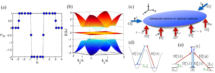
Figure 25: (Color online). (a) The topological invariant $\nu_{\text{w}}$ as a function of $h$. (b) Energy spectrum for three bulk bands (surface plot) and surface states (mesh plot) at the boundary along the $z$ direction for $h=2$. (c) Proposed scheme to realize the Hamiltonian (142). A linear tilt $\Delta_{x,y,z}$ per site in the lattice along each direction. The detuning in $x$ direction matches the frequency offset of the corresponding Raman beams, which are shown in panel (d). Polarizations of each beam are shown in brackets. Rabi frequencies for each beam are: $\Omega_{1}^{\pi}=\Omega_{0}e^{ikx}$, $\Omega_{2}^{\pi}=\Omega_{0}e^{iky}$, $\Omega_{1}^{x}=i\sqrt{2}\Omega_{0}e^{ikz}$, $\Omega_{2}^{x}=-i\sqrt{2}\Omega_{0}e^{ikz}$, $\Omega_{1}^{y}=-\sqrt{2}\Omega_{0}e^{ikz}$, $\Omega_{1}^{y}=\sqrt{2}\Omega_{0}e^{ikz}$, and $\Omega_{z}=2i\Omega_{0}e^{ikz}$. Reprinted with permission from Wang et al.[309]. Copyright©  (2014) by the American Physical Society.

To realize this model Hamiltonian, a three-species gas of noninteracting fermionic atoms (denoted by $|1\rangle$, $|2\rangle$ and $|3\rangle$) trapped in a 3D cubic OL is considered. The tight-binding Hamiltonian (142) in the real space has the following form

$$H =J\sum_{\mathbf{r}}[(2ihc^{\dagger}_{3,\mathbf{r}}c_{2,\mathbf{r}}+\text{H.c.})+H_{\mathbf{r\hat{x}}}+H_{\mathbf{r\hat{y}}}+H_{\mathbf{r\hat{z}}}],$$ (145)

$$H_{\mathbf{r\hat{x}}} =ic_{3,\mathbf{r-\hat{x}}}^{\dagger}(c_{1,\mathbf{r}}+c_{2,\mathbf{r}})-ic_{3,\mathbf{r+\hat{x}}}^{\dagger}(c_{1,\mathbf{r}}-c_{2,\mathbf{r}})+\text{H.c.},$$

$$H_{\mathbf{r\hat{y}}} =-c_{3,\mathbf{r-\hat{y}}}^{\dagger}(c_{1,\mathbf{r}}-ic_{2,\mathbf{r}})+c_{3,\mathbf{r+\hat{y}}}^{\dagger}(c_{1,\mathbf{r}}+ic_{2,\mathbf{r}})+\text{H.c.},$$

$$H_{\mathbf{r\hat{z}}} =2ic^{\dagger}_{3,\mathbf{r-\hat{z}}}c_{2,\mathbf{r}}+\text{H.c.}.$$

Here $c_{j,\mathbf{r}}(j=1,2,3)$ denotes the annihilation operator at the lattice site $\mathbf{r}$ with the spin state $|j\rangle$. The major difficulty for implementing this Hamiltonian is realization of the spin-transferring hopping terms $H_{\mathbf{r\hat{x}}}$,$H_{\mathbf{r\hat{y}}}$,$H_{\mathbf{r\hat{z}}}$. In principle, the required hopping can be realized by using the Raman-assisted tunneling with proper laser-frequency and polarization selections [26, 54, 114, 29, 30, 238].

A scheme to realize this Hamiltonian was proposed in Ref. [309]. As illustrated in Fig. 25(c), the atom-laser coupling configuration was suggested to realize the hopping terms, of which two beams $\Omega_{1}^{\pi}=\Omega_{0}e^{ikx}$ and $\Omega_{2}^{\pi}=\Omega_{0}e^{iky}$ constitute the $\pi$-polarized lights, propagating respectively along the $x$ and $y$ directions, where $k=2\pi/a$ is the magnitude of the laser wave vector. The other five beams $\Omega_{1,2}^{x,y,z}$ are all propagating along the $z$ direction with the polarizations shown in Fig. 25(c). Note that the required broken parity (left-right) symmetry is achieved by titling the lattice with a homogeneous energy gradient along the $x$-, $y$-, $z$-directions. A different linear energy shift per site $\Delta_{x,y,z}$ along different directions is required, such as $\Delta_{z}\approx 1.5\Delta_{y}\approx 3\Delta_{x}$. Then the natural hopping is suppressed by the large tilt potential, and the hopping terms are restored and engineered by applying two-photon Raman coupling with laser beams of proper configurations.

4.3.6 Hopf topological insulators

In general, 3D topological insulators should be protected by certain kinds of symmetries [123, 161], such as time-reversal, particle-hole, or chiral symmetries. However, a special class of 3D topological insulators without any symmetry other than the prerequisite $U(1)$ charge conservation was theoretically proposed, called Hopf insulators [66, 314, 315, 316, 294]. The Hopf insulator is topologically characterized by a topological invariant termed Hopf index (also known as Hopf charge or Hopf invariant) as discussed in Sec. A.7, and has zero Chern numbers. A two-band tight-binding model was first constructed on a cubic lattice to realize a special Hopf insulator with the Hopf index $\chi=1$ [66]. Subsequently, a class of tight-binding Hamiltonians that realize arbitrary Hopf insulator phases with any integer Hopf index $\chi$ were suggested [314]. Recently, an experimental scheme to implement a model Hamiltonian for Hopf insulators and to measure the Hopf topology in ultracold atomic systems has been proposed in Ref. [317]. The observation of topological links and Hopf fibration associated with Hopf insulators in a quantum simulator has been reported in Ref. [318].

The model Hamiltonian in momentum space discussed in Ref. [317] is given by

$$\mathcal{H}(\mathbf{k})=\bf S(\mathbf{k})\cdot\sigma,\leavevmode\nobreak\ \leavevmode\nobreak\ S(\mathbf{k})=\eta^{\dagger}\sigma\eta,$$ (146)

where $\bf S(\mathbf{k})$ is the pseudospin field. It is defined in terms of the two complex fields as $\eta=(\bar{\eta}_{\uparrow}^{p},\bar{\eta}_{\downarrow}^{q})^{t}$ with $p$ and $q$ being coprime integers, $\bar{\eta}_{\uparrow,\downarrow}=\eta_{\uparrow,\downarrow}^{*}$, where $\eta_{\uparrow}$ and $\eta_{\downarrow}$ are complex numbers given by

$$\eta_{\uparrow}(\mathbf{k})=\text{sin}{k_{x}}+i\text{sin}{k_{y}},\ \ \ \eta_{\downarrow}(\mathbf{k})=\text{sin}{k_{z}}+i(\text{cos}{k_{x}}+\text{cos}{k_{y}}+\text{cos}{k_{z}}+h),$$ (147)

with $h$ being a constant parameter. We introduce the standard $\text{CP}^{1}$ field $z(\mathbf{k})=\eta/\sqrt{|\bf S(\mathbf{k})|}=(z_{\uparrow}(\mathbf{k}),z_{\downarrow}(\mathbf{k}))^{t}$ and the normalized pseudospin ${\bf\hat{S}}(\mathbf{k})={\bf S(\mathbf{k})/|S(\mathbf{k})|}=z^{\dagger}\sigma{z}$ with $|{\bf S(\mathbf{k})}|=|\eta_{\uparrow}|^{2p}+|\eta_{\downarrow}|^{2q}$. It is easy to obtain the expression of $\bf\hat{S}(\mathbf{k})$,

$$\hat{S}_{x}+i\hat{S}_{y}={2\eta_{\uparrow}^{p}\bar{\eta}_{\downarrow}^{q}}/\eta_{+},\ \ \ \hat{S}_{z}={\eta_{-}}/{\eta_{+}},$$ (148)

where $\eta_{\pm}=|\eta_{\uparrow}|^{2p}\pm|\eta_{\downarrow}|^{2q}$. As we can see, the $\text{CP}^{1}$ field constructed by a four-component vector $N(\mathbf{k})$ with the configuration $N_{1}=\text{Re}[z_{\uparrow}(\mathbf{k})]$, $N_{2}=\text{Im}[z_{\uparrow}(\mathbf{k})]$, $N_{3}=\text{Re}[z_{\downarrow}(\mathbf{k})]$, and $N_{4}=\text{Im}[z_{\downarrow}(\mathbf{k})]$, takes values on the 3D sphere $\mathbb{S}^{3}$, together with the normalization condition $\sum_{i}N_{i}^{2}=1$. Therefore, Eq. (147) forms a map $g$: $\mathbb{T}^{3}\rightarrow\mathbb{S}^{3}$, where $\mathbb{T}^{3}$ is a 3D torus (describing the first BZ). On the other hand, the normalized pseudospin $\bf\hat{S}(\mathbf{k})$ expressed as $z^{\dagger}\sigma{z}$ defines a mapping $f$: $\mathbb{S}^{3}\rightarrow\mathbb{S}^{2}$, where the $\mathbb{S}^{3}$ coordinates $N(\mathbf{k})=(N_{1},N_{2},N_{3},N_{4})$ are mapped to $\mathbb{S}^{2}$ coordinates $(\hat{S}_{x},\hat{S}_{y},\hat{S}_{z})$. Consequently, the underlying structure of the Hamiltonian (146) constructs a composite map ${\bf\hat{S}}(\mathbf{k})=f\circ g(\mathbf{k})$: $\mathbb{T}^{3}\rightarrow\mathbb{S}^{2}$ from the BZ to the target pseudospin space $\mathbb{S}^{2}$.

The topological properties of the Hamiltonian in Eq. (146) are characterized by the Hopf index (see Sec. A.7), which has a simple integral expression [319, 67]

$$\nu_{H}({\hat{\bf S}})=-\int_{\text{BZ}}\mathbf{F}\cdot\mathbf{A}d^{3}{\bf k},$$ (149)

where $\bf F$ is the Berry curvature defined as ${\bf F}_{\mu}=\frac{1}{8\pi}\epsilon_{\mu\nu\tau}\hat{\bf S}\cdot(\partial_{\nu}\hat{\bf S}\times\partial_{\tau}\hat{\bf{S}})$ with $\epsilon_{\mu\nu\tau}$ being the Levi-Civita symbol and $\partial_{\nu,\tau}\equiv\partial_{k_{\nu,\tau}}(\mu,\nu,\tau\in\{x,y,z\})$, and $\bf A$ is the Berry connection that satisfies $\nabla\times{\bf A}=\bf F$. One can prove [314] that the Chern number $C_{\mu}=0$ in all three directions, and the Hopf index takes all integer values $\mathbb{Z}$ and has an analytic expression with $\nu_{H}(\hat{\bf S})=\pm pq$ when $1<|h|<3$, $\nu_{H}(\hat{\bf S})=\pm 2pq$ when $|h|<1$, $\nu_{H}(\hat{\bf S})=0$ otherwise. As we discussed before, $\hat{\bf S}(\mathbf{k})$ is a composition of two maps ${\bf\hat{S}}(\mathbf{k})=f\circ g(\mathbf{k})$. The generalized Hopf map $f$ from $\mathbb{S}^{3}\rightarrow\mathbb{S}^{2}$ has a known Hopf index $\chi(f)=\pm pq$ [319]. Thus, we can decompose the composition map, $\nu_{H}(\hat{\bf S})=\nu_{H}(f)\Lambda(g)$, where $\Lambda(g)$ is the topological invariant classifying the maps $g$ from $\mathbb{T}^{3}\rightarrow\mathbb{S}^{3}$

$$\Lambda(g)=\frac{1}{12\pi^{2}}\int_{\text{BZ}}d{\bf k}\epsilon_{\mu\nu\rho\tau}\frac{{\epsilon_{\alpha\beta\gamma}}}{|\boldsymbol{\eta}|^{4}}\eta_{\mu}\partial_{\alpha}\eta_{\nu}\partial_{\beta}\eta_{\rho}\partial_{\gamma}\eta_{\tau}.$$ (150)

Here $\boldsymbol{\eta}=(\text{Re}[\eta_{\uparrow}(\mathbf{k})],\text{Im}[\eta_{\uparrow}(\mathbf{k})],\text{Re}[\eta_{\downarrow}(\mathbf{k})],\text{Im}[\eta_{\downarrow}(\mathbf{k})])$. $\Lambda(g)=1$ when $1<|h|<3$, $\Lambda(g)=-2$ when $|h|<1$, and $\Lambda(g)=0$ otherwise. A geometric interpretation of such composition is as follows: $\Lambda(g)$ counts how many times $\mathbb{T}^{3}$ wraps around $\mathbb{S}^{3}$ nontrivially under the map $g$ and $\nu_{H}(f)$ describes how many times $\mathbb{S}^{3}$ wraps around $\mathbb{S}^{2}$ under $f$. This composite process ultimately gives the Hopf index $\nu_{H}(\hat{\bf S})$[314]. Numerical results show that the topologically protected surface states and zero-energy modes in these exotic nontrivial phases are robust against random perturbations [314, 66].

A geometrical image of the Hopf invariant can be obtained by noting that each point on $\mathbb{S}^{2}$ has a preimage that is a circle in $\mathbb{T}^{3}$, and that the linking number of two such circles taken from different points of $\mathbb{S}^{2}$ is the Hopf invariant $\nu_{H}(\hat{\bf S})$. To visualize such circles and knots more easily, one can work with $\mathbb{S}^{3}$ rather than $\mathbb{T}^{3}$ and probe the Hopf index $\nu_{H}(f)$. Similarly, the linking number of two preimage contours of distinct spin orientations is equal to the Hopf invariant $\nu_{H}(f)$. Nevertheless, $\mathbb{S}^{3}$ is a hypersphere in 4D space $\mathbb{R}^{4}$ where is difficult to visualize the circles in $\mathbb{S}^{3}$. So one can visualize the Hopf links by using a stereographic projection of $\mathbb{S}^{3}$ to $\mathbb{R}^{3}$, where the topological structure is retained [320, 321]. The stereographic projection used in Ref. [317] is defined as

$$(x,y,z)=\frac{1}{1+\eta_{4}}(\eta_{1},\eta_{2},\eta_{3}),$$ (151)

where $(x,y,z)$ and $(\eta_{1},\eta_{2},\eta_{3},\eta_{4})$ are points of $\mathbb{R}^{3}$ and $\mathbb{S}^{3}$, respectively. Stereographic projection preserves circles and maps of Hopf fibers as geometrically perfect circles in $\mathbb{R}^{3}$, but there is one exception: the Hopf circle containing the projection point $(0,0,0,-1)$ maps to a straight line in $\mathbb{R}^{3}$ as a “circle through infinity”. Moreover, the preimage map $f^{-1}(\hat{\bf S})$ in $\mathbb{S}^{3}$ must be determined in order to obtain the stereographic projection of the point on $\mathbb{S}^{3}$ in $\mathbb{R}^{3}$ by using Eq. (151). A direct parametrization of the 3D-sphere employing the Hopf map is as follows [319]

$$\eta_{\uparrow}=|\eta_{\uparrow}|e^{iq\theta_{1}},\ \ \ \eta_{\downarrow}=|\eta_{\downarrow}|e^{ip\theta_{2}},$$ (152)

or as follows in Euclidean $\mathbb{R}^{4}$

$$\eta_{1}=|\eta_{\uparrow}|\text{cos}(q\theta_{1}),\ \ \eta_{2}=|\eta_{\uparrow}|\text{sin}(q\theta_{1}),\ \ \eta_{3}=|\eta_{\downarrow}|\text{cos}(p\theta_{2}),\ \ \eta_{4}=|\eta_{\downarrow}|\text{sin}(p\theta_{2}),$$ (153)

where $\theta_{1,2}$ runs over the range $0$ to $2\pi$, with $|\eta_{\uparrow}|^{2}+|\eta_{\downarrow}|^{2}=1$. A mapping of the above parametrization to the 2D sphere (according to Eq. (148)) is given by

$$\hat{S}_{x}=\frac{2|\eta_{\uparrow}|^{p}|\eta_{\downarrow}|^{q}}{\eta_{+}}\text{cos}[pq(\theta_{1}-\theta_{2})],\ \hat{S}_{y}=\frac{2|\eta_{\uparrow}|^{p}|\eta_{\downarrow}|^{q}}{\eta_{+}}\text{sin}[pq(\theta_{1}-\theta_{2})],\ \hat{S}_{z}=\frac{\eta_{-}}{\eta_{+}}$$ (154)

For $\hat{\bf S}_{1}=(1,0,0)\big{(}\hat{\bf S}_{2}=(0,1,0)\big{)}$, we have $\theta_{1}=\theta_{2}\big{(}\theta_{1}=\theta_{2}+\frac{\pi}{2pq}\big{)}$, $|\eta_{\uparrow}|^{2p}=|\eta_{\downarrow}|^{2q}$. By combining it with the normalization condition $|\eta_{\uparrow}|^{2}+|\eta_{\downarrow}|^{2}=1$, we can obtain the values of $|\eta_{\uparrow}|$ and $|\eta_{\downarrow}|$. One can easily verify that $|\eta_{\uparrow}|^{2}=1$, $|\eta_{\downarrow}|^{2}=0$ $\big{(}|\eta_{\uparrow}|^{2}=0,|\eta_{\downarrow}|^{2}=1\big{)}$ for $\hat{\bf S}=(0,0,1)$ $\big{(}\hat{\bf S}=(0,0,-1)\big{)}$. With these preparations, we can check that a set of points ${\bf\eta}=(\text{cos}q\theta_{1},\text{sin}q\theta_{1},0,0)$ $\big{(}{\bf\eta}=(0,0,\text{cos}p\theta_{2},\text{sin}p\theta_{2})\big{)}$ forming a ring in $\mathbb{R}^{4}$ is the preimage of the point $\hat{\bf S}=(0,0,1)\big{(}\hat{\bf S}=(0,0,-1)\big{)}$ on $\mathbb{S}^{2}$. If we denote the stereographic projection $s$: $\mathbb{S}^{3}\backslash(0,0,0,-1)\rightarrow\mathbb{R}^{3}$ given in Eq. (151), then $s\circ f^{-1}((0,0,1))$ is the unit circle in the $x$-$y$ plane, $s\circ f^{-1}((0,0,-1))$ is the $z$ axis, and for any other point on $\mathbb{S}^{2}$ not equal to $(0,0,1)$ or $(0,0,-1)$, $s\circ f^{-1}(\hat{\bf S})$ is a circle in $\mathbb{R}^{3}$ when we choose $p=q=1$. In Fig. 26(a), the simplest nontrivial spin texture corresponding to $\nu_{H}(f)=1$ is sketched, where the parameters are chosen as $p=q=1$ and $h=2$. This spin texture twisted with $\nu_{H}(f)=1$ is nontrivial and cannot be continuously untwined unless a topological phase transition occurs. Following the above ideas, one can find more complex knots and links for larger $p$ and $q$, such as the well-known trefoil knot $(p=3,q=2)$ and the Solomon seal knot $(p=5,q=2)$ plotted in Ref. [317] with nonunit knot polynomials [322].

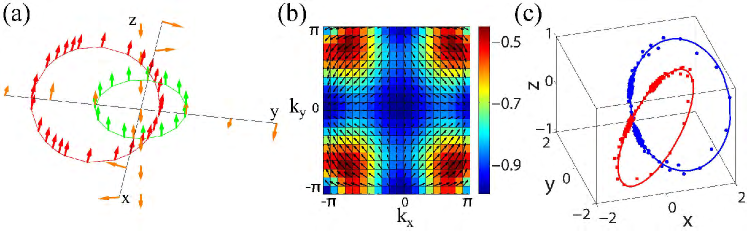
Figure 26: (Color online). (a) Hopf links and spin texture in stereographic coordinates. Spins residing on the red (green) circle point to the $x$ ($z$) direction and those on the $z$ axis all point to the south (negative $z$ direction). The red (green) circle represents the preimage of $\hat{\bf S}_{1}=(1,0,0)$ ($\hat{\bf S}_{2}=(0,0,1)$), and the $z$ axis represent the preimage of $(0,0,-1)$. (b)A cross-section of the measured spin texture along the $k_{z}=0$ layer. The background color scale labels the magnitude of the out-of-plane component $\hat{S}_{z}$, and the arrows label the magnitude and direction of spins in the $k_{x}$-$k_{y}$ plane. (c) Topological links between the preimages from two spin states on the Bloch sphere $\hat{\bf S}_{1}$ and $\hat{\bf S}_{2}$. The red (blue) circle denotes the theoretical preimage of $\hat{\bf S}_{1}$ ($\hat{\bf S}_{2}$) and the scattered red squares (blue dots) are numerically simulated preimage of the $\epsilon$-neighborhood of $\hat{\bf S}_{1}$ ($\hat{\bf S}_{2}$), which can be observed from time-of-flight images. The parameters are chosen as $p=q=1$ and $h=2$. Reprinted by permission from Deng et al.[317].

In the previous discussion, a nonvanishing value of $\nu_{H}(\hat{\bf S})$ indicates that the pseudospin field $\hat{\bf S}$ has a nontrivial texture that cannot be continuously deformed into a trivial one. Since the spin textures for the model can be interpreted as $\hat{\bf S}=\langle\sigma\rangle$, they can be observed in cold-atom experiments through time-of-flight imaging [244, 313]. Fig. 26(b) shows a slice of the observed $\hat{\bf S}$ with $k_{z}=0$ for the simplest case of $p=q=1$, which provides a glimpse of the 3D twisting of the Hopfion [323]. With the obtained spin texture, one can reconstruct the topological links and knots by mapping out the preimages of two different orientations of $\hat{\bf S}(\mathbf{k})$. However, the various kinds of noises involved in a real experiment may lead to inaccurate measurement results of $\hat{\bf S}(\mathbf{k})$. To simulate real experiments, the authors discussed the Hamiltonian (146) in real space and considered a finite-size lattice with open boundaries, so the spin orientation $\hat{\bf S}(\mathbf{k})$ in real experiment is always pixelized with a finite resolution, which means the observed $\hat{\bf S}(\mathbf{k})$ can only be approximately rather than exactly equal to the specific orientations (such as $\hat{\bf S}_{1,2}$) at any momentum point $\mathbf{k}$. To circumvent these difficulties, one need to consider a small $\epsilon$-neigborhood of a specific orientation (e.g., $\hat{\bf S}_{1}$):

$$N_{\epsilon}(\hat{\bf S}_{1})=\{\hat{\bf S}:|\hat{\bf S}-\hat{\bf S}_{1}|\leq\epsilon\},$$ (155)

where $|\hat{\bf S}-\hat{\bf S}_{1}|=[(\hat{S}_{x}-\hat{S}_{1x})^{2}+(\hat{S}_{y}-\hat{S}_{1y})^{2}+(\hat{S}_{z}-\hat{S}_{1z})^{2}]^{1/2}$ represents the distance between $\hat{\bf S}$ and $\hat{\bf S}_{1}$. The preimages of all orientations in $N_{\epsilon}(\hat{\bf S}_{1})$ are then denoted as a set of $P_{\epsilon}(\hat{\bf S}_{1})=(f\circ g)^{-1}[N_{\epsilon}(\hat{\bf S}_{1})]$ describing the points in $\mathbb{T}^{3}$. Due to the finite resolution and the discrete BZ, $P_{\epsilon}(\hat{\bf S}_{1})$ contains finite momentum points. Therefore, one should choose an appropriate value of $\epsilon$ to ensure that $P_{\epsilon}(\hat{\bf S}_{1})$ contains a proper amount of momentum points that could depict the closed loop structure of $(f\circ g)^{-1}(\hat{\bf S}_{1})$. Fig. 26(c) shows the simulated Hopf link with linking number one of real experiments. In order to obtain such images, one should first examine the discrete $\hat{\bf S}(\mathbf{k})$ at each momentum point $\mathbf{k}$ and then append $\mathbf{k}$ to the set of $P_{\epsilon}(\hat{\bf S}_{1})$ ($P_{\epsilon}(\hat{\bf S}_{2})$) while $\hat{\bf S}(\mathbf{k})$ is in an $\epsilon$-neighborhood of $\hat{\bf S}_{1}$ ($\hat{\bf S}_{2}$). By plotting $g(P_{\epsilon}(\hat{\bf S}_{1}))$ and $g(P_{\epsilon}(\hat{\bf S}_{2}))$ in the stereographic coordinate system defined in Eq. (151), one can obtain Fig. 26(c) in $\mathbb{R}^{3}$.

On the other hand, with the observed $\hat{\bf S}(\mathbf{k})$, one can directly extract the Hopf invariant. Since ${\bf F}_{\mu}=\frac{1}{8\pi}\epsilon_{\mu\nu\tau}\hat{\bf{S}}\cdot{\partial_{\nu}}\hat{\bf S}\times\partial_{\tau}\hat{\bf{S}}$, one can obtain the discrete Berry curvature $\bf F$ at each pixel of the BZ. Berry connection $\bf A(k)$ can be extracted from $\bf F$ by solving a discretized version of the electrostatics equation $\nabla\times\bf A=\bf F$ in momentum space with the Coulomb gauge $\nabla\cdot\bf A=0$. Finally, one can attain the value of the Hopf index $\nu_{H}(\hat{\bf S})$ by a discrete sum over all momentum points. It was also numerically demonstrated that a finite-size lattice of $10\times 10\times 10$ is already capable of producing highly accurate estimation of the quantized Hopf index and the detection method remains robust to experimental imperfections and the global harmonic trap [317].

The physical realization of the Hopf insulators is of great interest but also especially challenging. In principle, the model Hamiltonian of the Hopf insulators in Eq. (146) (with $p=q=1$ as the simplest case) could be realized using the Raman-assisted hopping technique with ultracold atoms in OLs, which will involve a number of laser beams [317].

4.3.7 Integer quantum Hall effect in 3D

After the discovery of the QHE in 2D systems [7, 8], it was shown that if there is a band gap in a 3D periodic lattice, the integer QHE can also exhibit when the Fermi energy lies inside the gap [324, 325, 326, 327]. In the 3D QHE, the Hall conductance in each crystal plane can have a quantized Hall value defined on a torus spanned by the two quasi-momenta for the crystal plane. It is hard to obtain the energy spectrum with band gaps for the emergence of quantized Hall conductivities in 3D periodic lattices since a motion along the third direction may wash out the gaps of the perpendicular 2D plane. Therefore up to now, the 3D QHE has been predicted or observed only in systems with extreme anisotropy or unconventional toroidal magnetic fields [328, 329, 327, 330, 331].

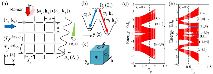
Figure 27: (Color online) A cold-atom setup for realizing a 3D generalized Hofstadter model [265]. (a) The OL and hopping configuration. Along the $s$ ($s=y,z$) axis, the tilted lattice with large tilt potentials $\Delta_{s}$ can be created by magnetic field gradients $B_{s}s$. The natural hopping along the $s$ axis is suppressed and then be restored by using three far-detuned Raman lasers denoted by $\{\omega_{j},\mathbf{k}_{j}\}$ ($j=1,2,3$), which give rise to complex hopping amplitudes $T_{y}e^{\pm i\phi_{m,n,l}}$ and $T_{z}e^{\pm i\varphi_{m,n,l}}$ with site indices ($m,n,l$). (b) Laser-assisted tunneling between nearest neighboring sites along the $s$ axis with the frequency differences $\omega_{2}-\omega_{1}=\Delta_{y}/\hbar$ and $\omega_{3}-\omega_{1}=\Delta_{z}/\hbar$ and the effective two-photon Rabi frequency $\Omega_{s}$. (c) The effective magnetic fluxes $\{\Phi_{1},\Phi_{2},\Phi_{3}\}$ in the three elementary plaquettes in the $\{xy,xz,yz\}$ planes, respectively. (d) (e) The energy spectra $E$ as a function of the hopping strength $T_{z}$ for (d) $\Phi_{1}=1/2$, $\Phi_{2}=1/3$, and $T_{y}=0.5$; (e) $\Phi_{1}=1/3$, $\Phi_{2}=1/5$, and $T_{y}=0.5$. The dashed lines are shown in (d) with $T_{z}=0.7$ and in (e) with $T_{z}=0.5$. The Chern numbers $\mathbf{C}=(C_{xy},C_{xz},C_{yz})$ when the Fermi level lies in each energy gap are shown. Reprinted with permission from Zhang et al.[265]. Copyright© (2017) by the American Physical Society.

A scheme was recently proposed to realize the 3D QHE in a tunable generalized 3D Hofstadter system that can be simulated by engineering the Raman-assisted hopping of ultracold atoms in a cubic OL [265]. The optical lattice is tilted along the $y$ and $z$ axis, as shown in Fig. 27(a). The atoms are prepared in a hyperfine state of the ground state manifold, and the tilt potentials with linear energy shift per lattice site $\Delta_{s}$ ($s=y,z$) can be generated by the gravity or real magnetic field gradients $B_{s}s$. For the case $\Delta_{s}\gg J_{s}$ we considered, where $J_{s}$ denotes the bare hopping amplitude along the $s$ axis, the atomic hopping between neighboring sites in these two directions is suppressed. To restore and engineer the hopping terms with tunable effective phases, we can use the Raman-assisted tunneling technique, which has been used to realize the original Hofstadter model in 2D OLs [29, 30, 48]. In order to fully and independently engineer the atomic hopping along the $y$ and $z$ axes, one can use three far-detuned Raman beams denoted by their frequencies and wave vectors $\{\omega_{j},\mathbf{k}_{j}\}$ ($j=1,2,3$), as shown in Fig. 27(b). For resonant tunneling along different directions, the frequency differences $\omega_{2}-\omega_{1}=\Delta_{y}/\hbar$ and $\omega_{3}-\omega_{1}=\Delta_{z}/\hbar$ with $\Delta_{y}\neq\Delta_{z}$ are required. The momentum transfers $\mathbf{Q}=\mathbf{k_{1}}-\mathbf{k_{2}}\equiv(Q_{x},Q_{y},Q_{z})$ and $\mathbf{P}=\mathbf{k_{1}}-\mathbf{k_{3}}\equiv(P_{x},P_{y},P_{z})$ can be independently tunable, for instance, through independently adjusting the angles of the second and third Raman lasers with the first Raman laser being fixed, as shown in Fig. 27(a). Therefore, the Raman lasers induce atomic hopping along the $y$ and $z$ axes with tunable, spatially dependent phases $\phi_{m,n,l}=\mathbf{Q}\cdot\mathbf{R}=m\phi_{x}+n\phi_{y}+l\phi_{z}$ and $\varphi_{m,n,l}=\mathbf{P}\cdot\mathbf{R}=m\varphi_{x}+n\varphi_{y}+l\varphi_{z}$, respectively, where $\mathbf{R}=(ma,na,la)$ denotes the position vector for the lattice site $(m,n,l)$, $\phi_{x,y,z}=aQ_{x,y,z}$ and $\varphi_{x,y,z}=aP_{x,y,z}$. This system realizes a generalized 3D Hofstadter Hamiltonian with fully tunable hopping parameters [265]

$$H=-\sum_{m,n,l}[J_{x}a^{\dagger}_{m+1,n,l}a_{m,n,l}+e^{i\phi_{m,n,l}}(T_{y}a^{\dagger}_{m,n+1,l}a_{m,n,l}+T_{z}a^{\dagger}_{m,n,l+1}a_{m,n,l})+\text{H.c.}],$$ (156)

where $J_{x}$ is the natural hopping along the $x$ axis, $T_{y}e^{i\phi_{m,n}}$ ($T_{z}e^{i\varphi_{m,l}}$) denotes the Raman-induced hopping along the $y$ ($z$) axis with the spatially-varying phase $\phi_{m,n}$ ($\varphi_{m,l}$) imprinted by the Raman lasers. The hopping strengths $T_{s}=\Omega_{s}\lambda_{s}$ can also be tuned via the laser intensities, with $\lambda_{s}$ denoting the overlap integral of Wannier-Stark functions between neighbor sites along the $s$ axis. One can introduce three effective magnetic fluxes $\{\Phi_{1},\Phi_{2},\Phi_{3}\}$ through the three elementary plaquettes in the $\{xy,xz,yz\}$ planes with the area $S=a^{2}$, as shown in Fig. 27(c). The effective fluxes, in units of the magnetic flux quantum, are determined by the phases picked up anticlockwise around the plaquettes. They are obtained as $\Phi_{1}=\frac{\phi_{x}}{2\pi}$, $\Phi_{2}=\frac{\varphi_{x}}{2\pi}$, and $\Phi_{3}=\frac{\phi_{z}-\varphi_{y}}{2\pi}$, which can be independently tuned. For certain hopping configurations, the bulk bands of the system can respectively have Weyl points and nodal loops [265], similar as the one proposed in Ref. [264]. This allows the study of both nodal semimetal states within this cold atom system. Furthermore, the system can exhibit the 3D QHE when the Fermi level lies in the band gaps, which is topologically characterized by one or two nonzero Chern numbers.

For simplicity, we consider $\Phi_{3}=0$ and rational fluxes $\Phi_{1}=p_{1}/q_{1}$ and $\Phi_{2}=p_{2}/q_{2}$, with mutually prime integers $p_{1,2}$ and $q_{1,2}$. In this case, the Hamiltonian (156) can be block diagonalized as ${H}=\bigoplus{H}_{x}(k_{y},k_{z})$, where $k_{y}$ and $k_{z}$ are the quasimomenta along the periodic directions and the decoupled block Hamiltonian is given by

$${H}_{x}(k_{y},k_{z})=-\sum_{m}(J_{x}a^{\dagger}_{m+1}a_{m}+\text{H.c.})-\sum_{m}V_{m}a^{\dagger}_{m}a_{m},$$ (157)

where $V_{m}=2T_{y}\text{cos}(2\pi\Phi_{1}m+k_{y}a)+2T_{z}\text{cos}(2\pi\Phi_{2}m+k_{z}a)$. The corresponding single-particle wave function $\Psi_{mnl}$ is written as $\Psi_{mnl}=e^{ik_{y}y+ik_{z}z}\psi_{m}$, and then the Schrödinger equation $\hat{H}_{x}(k_{y},k_{z})\Psi_{mnl}=E\Psi_{mnl}$ reduces to a generalized Harper equation:

$$-J_{x}(\psi_{m-1}+\psi_{m+1})-V_{m}\psi_{m}=E\psi_{m}.$$

This 1D reduced tight-binding system with two commensurabilities $\Phi_{1}$ and $\Phi_{2}$ has a period of the least common multiple of integers $q_{1}$ and $q_{2}$ denoted by $\tilde{q}=[q_{1},q_{2}]$. Under the periodic boundary condition along the $x$ axis, the wave function $\psi_{m}$ satisfies $\psi_{m}=e^{ik_{x}x}u_{m}(\mathbf{k})$ with $u_{m}(\mathbf{k})=u_{m+\tilde{q}}(\mathbf{k})$. Therefore in a general case, the spectrum of the three-dimensional system in the presence of the effective magnetic fluxes consists of $\tilde{q}$ energy bands and each band has a reduced (magnetic) BZ: $-\pi/\tilde{q}a\leq k_{x}\leq\pi/\tilde{q}a$, $-\pi/a\leq k_{y}\leq\pi/a$, and $-\pi/a\leq k_{z}\leq\pi/a$. In term of the reduced Bloch wave function $u_{m}(\mathbf{k})$, one has $-J_{x}(e^{ik_{x}}u_{m-1}+e^{-ik_{x}}u_{m+1})-V_{m}u_{m}=E(\mathbf{k})u_{m}$.

It was proven that every quantized invariant on a $d$-dimensional torus $\mathbb{T}^{d}$ is a function of the $d(d-1)/2$ sets of Chern numbers obtained by slicing $\mathbb{T}^{d}$ by the $d(d-1)/2$ distinct $\mathbb{T}^{2}$ [332]. In this 3D Hofstadter system, the topological invariants for the QHE are given by three Chern numbers $\mathbf{C}=(C_{xy},C_{xz},C_{yz})$ for three 2D planes, with $C_{yz}=0$ for the trivial $yz$ plane since $\Phi_{3}=0$. As with the approach in Refs. [325, 326], when the Fermi energy lies in an energy gap between two bands $N$ and $N+1$ in this system, the other two Chern numbers $C_{xs}$ with $s=y,z$ are given by

$$C_{xs}=\frac{1}{2\pi}\sum_{n\leqslant N}\int_{-\pi}^{\pi}dk_{s^{\prime}}c_{xs}^{(n)}(k_{s^{\prime}}),$$ (158)

where $s^{\prime}$ denotes replacing $s$ between $y$ and $z$, and the Chern number $c_{xs}^{(n)}(k_{s^{\prime}})$ for the $n$-th filling band (or $n$-th occupied Bloch state) is defined on the torus $T^{2}$ spanned by $k_{x}$ and $k_{s}$: $c_{xs}^{(n)}(k_{s^{\prime}})=\frac{1}{2\pi}\int_{-\pi/\tilde{q}}^{\pi/\tilde{q}}dk_{x}\int_{-\pi}^{\pi}dk_{s}F_{xs}^{(n)}(\textbf{k})$, where $F_{xs}^{(n)}(\textbf{k})$ is the corresponding Berry curvature as a topological expression as a generalization of the results in 2D [10]. In Figs. 27(d) and (e), the three Chern numbers $\mathbf{C}=(C_{xy},C_{xz},C_{yz})$ when the Fermi level lies in each energy gap and the spectra are plotted. The results demonstrate that the QHE in this 3D Hofstadter system is topologically characterized by one or two nonzero Chern numbers.

4.4 Higher and synthetic dimensions

An important development in exploration of topological states with ultracold atomic gases is the concept of “synthetic dimensions”. As discussed in Sec. 4.1.5, the topological properties of 1D quasiperiodic OLs described by the Aubry-André-Harper model can be mapped to the 2D QHE. A key in the mapping is that a cyclical parameter adiabatically varying from $0$ to $2\pi$ in the 1D lattice (such as the phase of the lattice potential) plays the role of the quasimomentum of the second dimension. In Thouless pumping, the 1D system constitutes a Fourier component of a 2D quantum Hall system at each point of the cycle, where an adiabatic periodic pump parameter also acts as the quasimomentum. In these cases, the cyclical parameter can effectively be considered a synthetic dimension under the periodic boundary condition along this dimension. This approach can be extended to studying topological systems in higher dimensions $D=d_{r}+d_{s}\geqslant 3$ in OLs of real spatial dimensions $d_{r}=\{1,2,3\}$ and synthetic dimensions $d_{s}$. For example, it was proposed to simulate 3D Weyl semimetal physics with cold atoms in $d_{r}=\{2,1\}$D OLs that are subjected to $d_{s}=\{1,2\}$D synthetic dimensions from external cyclical parameters [256, 136]. More interestingly, the intriguing 4D quantum Hall physics [16, 64] can be explored in a 2D topological charge pump in 2D OLs with two cyclical parameters, which together give an effective 4D BZ [333, 334, 17].

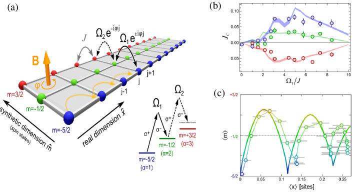
Figure 28: (Color online) (a) A synthetic gauge field in a synthetic dimension. ¹⁷³Yb fermionic atoms are loaded in a hybrid lattice, generated by an OL along a real direction $\hat{x}$ with tunneling $J$, and by a Raman-induced hopping between nuclear spin states along a synthetic direction $\hat{m}$ with a complex tunneling $\Omega_{1,2}e^{i\varphi j}$. (b) Experimental observation of chiral edge currents $J_{c}$. (c) Experimental observation of edge-skipping orbits in the ladder. Reprinted from Manciniet al.[37]. Reprinted with permission from AAAS.

Another kind of synthetic dimension is engineered by a set of discrete internal atomic (spin) states as fictitious lattice sites [335, 336]. In this approach, the atoms loaded into a $d_{r}$-dimensional OL can potentially simulate systems of $D=d_{r}+1$ spatial dimensions. The hopping processes along the synthetic dimension can be induced by driving transitions between different internal states with Raman lasers. The laser-coupling between two internal atomic states has complex coupling element, which represents the tunneling matrix in the synthetic dimension picture. Hence, similar to the Raman-assisted-tunneling scheme, this fictitious tunneling contains a complex phase-factor, which can then be used to simulate synthetic gauge fields in the synthetic dimensions and a finite strip of the Hofstadter model [336]. For the atoms that have the hyperfine spin $F$, the Raman lasers couple spin state $|m_{F}\rangle$ to $|m_{F}\pm 1\rangle$, where $m_{F}$ takes any value between $-F$ and $F$ with a total of $W=2F+1$ components. This provides the naturally sharp boundaries in the extra dimension, while it is also possible to create periodic boundary conditions in the synthetic dimension by using an additional coupling to connect the extremal internal states. This differs from the cyclical synthetic dimension previously introduced. Therefore, the proposed 1D OL [336] that combines real and synthetic spaces offers a key advantage to work with a finite-sized system with sharp and addressable edges, such as the detection of chiral edge states resulting from the synthetic magnetic flux.

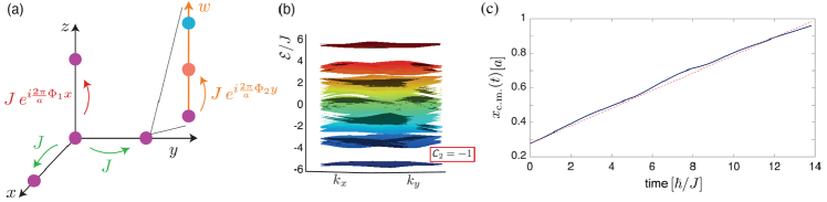
Figure 29: (Color online) (a) The synthetic 4D lattice in the absence of perturbing fields, with atoms in a 3D OL with hopping amplitude $J$ and flux $2\pi\Phi_{1}$ from $x$-dependent Peierls phase-factors in $z$ hopping. The fourth dimension $w$ is a synthetic dimension with flux $2\pi\Phi_{2}$ in the $y\!-\!w$ plane by adding a $y$-dependent phase-factor to the Raman-induced internal-state transitions. (b) Energy spectrum $\mathcal{E}(k_{x},k_{y})$ for $\Phi_{1,2}\!=\!1/4$ and for many values $k_{z,w}$, with the second Chern number of the lowest band $C_{2}\!=\!-1$. (c) Simulation of the center-of-mass trajectory $x_{\text{c.m.}}(t)$ after ramping up a perturbing “electric” and “magnetic” field (the blue sold curve), with the predicted drift for $C_{2}\!=\!-1$ (the red dotted curve). Reprinted with permission from Price et al.[41]. Copyright© (2015) by the American Physical Society.

The proposed synthetic-dimension scheme [336] was recently realized in two independent experiments with ¹⁷³Yb fermionic atoms [37] and ⁸⁷Rb bosonic atoms [38]. As shown in Fig. 28(a), a system of ¹⁷³Yb fermionic atoms in an atomic Hall ribbon of tunable width pierced by an effective gauge field was experimentally synthesized [37]. One real dimension is realized by an OL with the tunneling $J$ between different sites along direction $\hat{x}$. The synthetic dimension is encoded in the different internal spin states (the sites of the synthetic dimension for the $F=5/2$ nuclear spin manifold are up to six), which are coupled by a two-photon Raman transition with a coherent controllable coupling $\Omega e^{i\varphi x}$ between different spin components. The phase amounts to the synthesis of an effective magnetic field with tunable flux $\varphi/2\pi$ (in units of the magnetic flux quantum) per plaquette, mimicking the 2D Hofstadter model on a three-leg ladder. The Hamiltonian of the system is given by

$$H=\sum_{j}\sum_{\alpha}\left[-J(c^{\dagger}_{j,\alpha}c_{j+1,\alpha}-\frac{\Omega_{\alpha}}{2}e^{i\varphi j}c^{\dagger}_{j,\alpha}c_{j,\alpha+1}+\textrm{h.c.})+\mu_{j}n_{j,\alpha}+\xi_{\alpha}n_{j,\alpha}\right],$$ (159)

where $c^{\dagger}_{j,\alpha}(c_{j,\alpha})$ are fermionic creation (annihilation) operators on the site $(j,\alpha)$ in the real ($j$) and synthetic ($\alpha=1,2,3$) dimension, and $n=c^{\dagger}_{j,\alpha}c_{j,\alpha}$. The hopping parameters $\Omega_{\alpha}$ are typically inhomogeneous due to the Clebsch-Gordan coefficients associated with the atomic transitions. Besides the tunneling terms, $\mu_{j}$ describes a weak trapping potential along $\hat{x}$, while $\xi_{\alpha}$ accounts for a state-dependent light shift, giving an energy offset along $\hat{m}$. In the experiment, the chiral currents $J_{c}$ in the upper and lower edge chains with opposite sign were observed, while the central leg showed a suppressed net current in the bulk, as shown in Fig. 28(b). This directly signals the existence of chiral states propagating along the edges of the system, reminiscent of the edge states in the QHE in the Hofstadter model. In addition, the edge-skipping orbits with the cyclotron-type dynamics in the ladder due to the presence of the synthetic magnetic field were further detected through state-resolved images of the atomic cloud, as shown in Fig. 28(c). In the ladders, the finite-size effect (such as the overlap of chiral edge modes in different edges) is significant because the lattice size along the synthetic dimension is small. To limit undesired finite-size effects, one may use other atomic species with more addressable internal states in the synthetic-dimension approach.

The synthetic three-leg ladder with the magnetic flux was also realized for ⁸⁷Rb bosonic atoms, and the chiral edge currents and skipping orbits were both observed in the quantum Hall regime [38]. In addition, this synthetic-dimension approach was demonstrated in a more recent experiment without two-photon Raman transitions but instead, based on a single-photon optical clock transition coupling two long-lived electronic states of two-electron ¹⁷³Yb atoms [39]. These two systems involve less heating, which would be important for further studies, such as spectroscopic measurements of the Hofstadter butterfly and realizations of Laughlin’s charge pump.

There is an important difference between ordinary lattice systems and systems involving a synthetic dimension. In the synthetic dimension, interactions are generically long-ranged, in contrast to the on-site interactions along the physical dimension. With the effectively nonlocal interactions, the cold atom systems realize extended-Hubbard models, which can display novel phases due to the intriguing many-body effects unattainable in conventional condensed matter setups [337, 338, 339, 340]. Such an interacting fermion gas with multi-spin components coupled through Raman beams in a 1D OL provides an ideal system to realize the topological fractional pumping reflected by the quantization to fractional values of the pumped charge and to measure the many-body Chern number in a cold-atom experiment [341, 153].

The synthetic-dimension technique offers a novel platform for exploring topological states in higher dimensions [16, 40], such as detecting the 4D QHE [41]. In the 2D QHE, the quantized Hall response induced by an external electric field is topologically characterized by the first Chern number. As one of the first predictions of the time-reversal symmetric topological insulators [16, 64], the QHE can be generalized to 4D systems. In the 4D QHE, an additional quantized Hall response appears, which is nonlinear and described by a 4D topological index, the second Chern number. The intriguing 4D QHE with the second Chern number was also theoretically studied in other models [64, 342, 343, 333]. In the proposal [41], as shown in Fig. 29(a), a synthetic 4D lattice contains atoms hopping in a 3D OL with Raman-coupling internal states as the fourth dimension $w$, in which the $x\!-\!z$ and $y\!-\!w$ planes are penetrated by synthetic uniform magnetic fluxes $\Phi_{1,2}$, respectively. This corresponds to two copies of the Hofstadter model defined in disconnected planes, described by the tight-binding Hamiltonian

$$H_{4\text{D}}=-J\sum_{\boldsymbol{r}}\big{(}c^{\dagger}_{\boldsymbol{r}+a\boldsymbol{e}_{x}}c_{\boldsymbol{r}}+c^{\dagger}_{\boldsymbol{r}+a\boldsymbol{e}_{y}}c_{\boldsymbol{r}}+e^{i2\pi\Phi_{1}x/a}c^{\dagger}_{\boldsymbol{r}+a\boldsymbol{e}_{z}}c_{\boldsymbol{r}}+e^{i2\pi\Phi_{2}y/a}c^{\dagger}_{\boldsymbol{r}+a\boldsymbol{e}_{w}}c_{\boldsymbol{r}}\big{)}+\text{h.c.},$$ (160)

where $c^{\dagger}_{\boldsymbol{r}}$ creates a fermion at lattice site $\boldsymbol{r}\!=\!(x,y,z,w)$. To realize this Hamiltonian, one requires $x$ ($y$) dependent Peierls phases for tunneling along the $z$ ($w$) direction, generating a uniform flux $\Phi_{1}$ ($\Phi_{2}$) in the $x\!-\!z$ ($y\!-\!w$) plane. This can be created by combining the laser-assisted hopping along the $z$ direction and the synthetic gauge field in the synthetic dimension. As shown in Fig. 29(b), the bulk energy spectrum $\mathcal{E}(\boldsymbol{k})$ of the Hamiltonian is reminiscent of the two underlying 2D Hofstadter models defined in the $x\!-\!z$ and $y\!-\!w$ planes, where the lowest band can be non-degenerate and well isolated from higher-energy bands for suitable fluxes $\Phi_{1,2}$. Moreover, the lowest band $\mathcal{E}_{1}(\boldsymbol{k})$ is characterized by a non-zero second Chern number $C_{2}=-1$ from [41]

$$C_{2}\!=\!\frac{1}{4\pi^{2}}\int_{\mathbb{T}^{4}}(\Omega^{xy}\Omega^{zw}\!+\!\Omega^{wx}\Omega^{zy}\!+\!\Omega^{zx}\Omega^{yw})\text{d}^{4}k,$$ (161)

where $\Omega^{\mu\nu}$ is the 4D generalized Berry curvature. If there are additional perturbing “electric” field $\!E_{y}$ and “magnetic” field $B_{zw}\!=-\!2\pi\tilde{\Phi}/a^{2}$, the current density along the $x$ dimension as a response for a filled band is given by

$$j^{x}=\frac{C_{2}}{4\pi^{2}}E_{y}B_{zw}=-\frac{C_{2}}{2\pi a^{2}}E_{y}\tilde{\Phi},$$ (162)

which reveals a genuine non-linear 4D quantum Hall response and is directly related to $C_{2}$. Hence, as shown in Fig. 29(c), the second Chern number in this system can be measured from the center-of-mass drift along the $x$ direction [41, 344]: $x_{\text{c.m.}}(t)=x_{\text{c.m.}}(0)+v_{\text{c.m.}}t=x_{\text{c.m.}}(0)+j^{x}V_{\text{cell}}t$, with $V_{\text{cell}}$ as the (magnetic) unit cell volume. For the neutral atoms, the perturbing “electric” field corresponds to a linear gradient that can created either magnetically or optically, and the perturbing “magnetic” field can be generated by engineering additional Peierls phases.

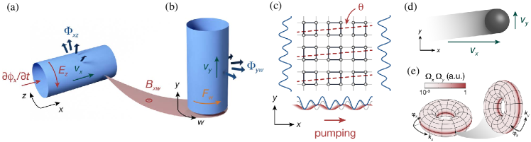
Figure 30: (Color online) 4D quantum Hall system and corresponding 2D topological charge pump. (a) A 2D quantum Hall system on a cylinder pierced by a uniform magnetic flux $\Phi_{xz}$, and an electric field $E_{z}$ on the surface resulting in a linear Hall response along $x$ with velocity $v_{x}$. (b) A 4D quantum Hall system can be composed of two 2D quantum Hall systems in the $xz$- and $yw$-planes. (c) A dynamical version of the 4D quantum Hall system can be realized with a topological charge pump in a 2D superlattice (blue potentials). (d) The pumping gives rise to a motion of the atom cloud in the $x$-direction, corresponding to the quantized linear response of a 2D quantum Hall system. (e) The velocity of the non-linear response is determined by the product of the Berry curvatures $\Omega^{x}\Omega^{y}$. The left (right) torus shows a cut at $k_{y}=0$, $\varphi_{y}=\pi/2$ ($k_{x}=\pi/(2d_{l})$, $\varphi_{x}=\pi/2$) through the generalized 4D BZ spanned by $k_{x,y}$ and $\varphi_{x,y}$. Reprinted by permission from Macmillan Publishers Ltd: Lohse et al. [17], copyright© (2018).

Recently, based on a 2D topological charge pump as proposed in Ref. [333], a dynamical version of the 4D integer QHE was realized by using ultracold bosonic atoms in an angled optical superlattice, and the bulk quantized response associated with the second Chern number was observed [17]. The dynamical 4D quantum Hall system was also experimentally realized with tunable 2D arrays of photonic waveguides [334]. For the geometry in Figs. 30(a,b), the 2D subsystem as a Fourier component of a 4D quantum Hall system is a square superlattice in Fig. 30(c). It consists of two 1D superlattices along $x$ and $y$, each formed by superimposing two lattices $V_{s,\mu}\text{sin}^{2}\left(\pi\mu/d_{s}\right)+V_{l,\mu}\text{sin}^{2}\left(\pi\mu/d_{l}-\varphi_{\mu}/2\right)$, where $\mu\in\{x,y\}$, $d_{s,\mu}$, and $d_{l,\mu}=2d_{s,\mu}$ denote the lattice periods, and $V_{s,\mu}$ ($V_{l,\mu}$) is the depth of the short (long) lattice potential. The superlattice phases $\varphi_{\mu}$ determined the position of the long lattices relative to the short ones, and the phase $\varphi_{x}$ was chosen as the pump parameter in the experiment [17]. This is equivalent to threading $\varphi_{x}$ in the 4D model, which leads to a quantized motion along $x$ as the linear response shown in Figs. 30(c,d). The magnetic perturbation $B_{xw}$ corresponds to a transverse superlattice phase $\varphi_{y}$ that depends linearly on $x$, which is realized by tilting the long $y$-lattice relative to the short one by a small angle $\theta$ in the $xy$-plane, with $\varphi_{y}(x)=\varphi_{y}^{(0)}+2\pi\theta\,x/d_{l,y}$ to first order in $\theta$. As the two orthogonal axes are coupled, by varying $\varphi_{x}$, the motion along $x$ changes $\varphi_{y}$. This is analogous to the Lorentz force in 4D and induces a quantized non-linear response along $y$ [333]. For a uniformly populated band in an infinite system, the change in the center-of-mass position $\Delta{\boldsymbol{r}}$ during one cycle $\varphi_{x}=0\rightarrow 2\pi$ is given by [17]

$$\Delta{\boldsymbol{r}}=C_{1}^{x}\,d_{l,x}\,\mathbf{e}_{x}+C_{2}\,\theta\,d_{l,x}\,\mathbf{e}_{y}.$$ (163)

The first term proportional to the pump’s first Chern number $C_{1}^{x}$ describes the quantized linear response in the $x$-direction. The second term is the non-linear response in the $y$-direction, which is quantified by a 4D integer topological invariant, the pump’s second Chern number

$$C_{2}=\frac{1}{4\pi^{2}}\oint_{BZ}\Omega^{x}\Omega^{y}\mathrm{d}k_{x}\mathrm{d}k_{y}\mathrm{d}\varphi_{x}\mathrm{d}\varphi_{y}.$$ (164)

The generalized 4D BZ is shown in Fig. 30(e), and the Berry curvature $\Omega^{\mu}(k_{\mu},\varphi_{\mu})=i\left(\langle{\partial_{\varphi_{\mu}}u}|{\partial_{k_{\mu}}u}\rangle-\langle{\partial_{k_{\mu}}u}|{\partial_{\varphi_{\mu}}u}\rangle\right)$, with $|{u(k_{\mu},\varphi_{x})}\rangle$ as the eigenstate of a given non-degenerate band at $k_{\mu}$ and $\varphi_{\mu}$. In the experiment [17], the 2D topological charge pump was realized with bosonic ⁸⁷Rb atoms forming a Mott insulator in the superlattice. The 4D-like nonlinear response of the lowest subband with $C_{2}=+1$ was experimentally observed from the atomic center-of-mass shift after a pump circle. Furthermore, using a small cloud of atoms as a local probe, the 4D geometric properties and the quantization of the response were fully characterized via in situ imaging and site-resolved band mapping. This work paves the way for exploring higher-dimensional quantum Hall systems with additional strongly correlated topological phases, exotic collective excitations and boundary phenomena such as isolated Weyl fermions [16, 64].

Finally we note that the concept of synthetic dimension has been greatly extended, which can involve other kinds of degrees of freedom. For instance, the synthetic dimensions may also be engineered by a set of orbital angular momenta for light [345] or harmonic oscillator eigenstates for cold atoms in a harmonic trap [346] as fictitious lattice sites. Moreover, it was proposed to create an effective synthetic lattice of sites in momentum space based on discrete momentum states of neutral atoms, which can be parametrically coupled with interfering Bragg laser fields [143, 144]. The synthetic momentum-space lattice has been realized with cold atoms and opened up new prospects in the experimental study of disordered and topological systems [142, 145, 347, 348, 349].

4.5 Higher-spin topological quasiparticles

In the previous sections, we focus on the spin-1/2 systems, such as the Dirac and Weyl fermions, which have rich topological features. Quasiparticles with higher spin numbers are also fundamentally important but rarely studied in condensed-matter physics or artificial systems [350, 351, 352]. These systems can potentially provide a quantum family to find relativistic quasiparticles that have no high-energy analogs, such as integer-(speudo)spin fermionic excitations. Recently, a series of work theoretically predicted that unconventional fermions beyond the Dirac-Weyl-Majorana classification (also termed “new fermions”, which means no elementary particle analogs) can emerge in some band structures [350, 353]. These works have set off a boom in investigating and realizing “new fermions” in condensed matter and artificial systems [354, 355, 356, 357, 358, 359, 360, 361].

A recent work to implement the pseudospin-1 fermions in cold-atom systems was proposed in Ref. [355]. In this paper, the authors constructed 2D and 3D tight-binding models realizable with cold fermionic atoms in OLs, where the low-energy excitations are effectively described by the spin-1 Maxwell equations in the Hamiltonian form. The Hamiltonian of these low-energy excitations is given by

$$H_{M}=v_{x}k_{x}\hat{S}_{x}+v_{y}k_{y}\hat{S}_{y}+v_{z}k_{z}\hat{S}_{z},$$ (165)

where $\hat{S}_{\beta}=(\hat{S}_{\alpha\gamma})^{\beta}=i\epsilon_{\alpha\beta\gamma}$, and $\epsilon_{\alpha\beta\gamma}$ $(\alpha,\beta,\gamma=x,y,z)$ is the Levi-Civita symbol. This so-called Maxwell Hamiltonian $H_{M}$ originally describes a massless relativistic boson (photon) with spin one. Because quasiparticles in a lattice system are constrained only by certain subgroups (space groups) of the Poincaré symmetry rather than by Poincaré symmetry in high-energy physics [350], there is the potential to find free fermionic excitations described by $H_{M}$ in lattice systems. Such relativistic (linear dispersion) excitations with unconventional integer pseudospins are termed Maxwell fermions. For specificity and without loss of generality, we describe the topological features of Maxwell fermions in 2D and 3D OLs in some detail.

The proposed Bloch Hamiltonian for a 2D case in momentum space is as follows [355]

$$\mathcal{H}(\mathbf{k})=\mathbf{R}(\mathbf{k})\cdot\hat{\bf S}$$ (166)

where the Bolch vector ${\bf R}(\mathbf{k})=(R_{x},R_{y},R_{z})$ is given by

$$R_{x}=2J\leavevmode\nobreak\ \text{sin}k_{x},\ \ R_{y}=2J\leavevmode\nobreak\ \text{sin}k_{y},\ \ R_{z}=2J(M-\text{cos}k_{x}-\text{cos}k_{y}),$$ (167)

with $M$ being a tunable parameter. The energy spectrum of this system is given by $E(\mathbf{k})=0,\pm|\mathbf{R}(\mathbf{k})|$, which has a zero-energy flat band in the middle of the three bands. The three bands touch at a single point $\mathbf{K}_{\pm}=(0,0)/(\pi,\pi)$ when $M=\pm 2$, as shown in Fig. 31(a), and touch at two points when $M=0$. The low-energy effective Hamiltonian near $\mathbf{K}_{\pm}$ can be expanded to linear order as

$$\mathcal{H}_{\pm}(q)=\pm v(q_{x}\hat{S}_{x}+q_{y}\hat{S}_{y}),$$ (168)

where $v=2J$ is the effective speed of light and $\mathbf{q}=\mathbf{k}-\mathbf{K}_{\pm}$. These fermionic excitations are described by the Maxwell Hamiltonian $H_{M}$ in 2D. In this sense, these low-energy excitations can be named Maxwell fermions, and the threefold degenerate point as Maxwell point. When the Fermi level lies near the Maxwell point, this system is also named Maxwell metal with a zero-energy flat band. To study the topological properties of Maxwell metal phase, one can evaluate the Berry phase circling around the Maxwell point $\gamma=\oint_{c}d\mathbf{k}\cdot\mathbf{\mathbf{F}(k)},$ where the Berry curvature $\mathbf{F(k)}$ for the lower band in the $k_{x}$-$k_{y}$ space has an expression of

$$F_{xy}=-\frac{1}{R^{3}}\mathbf{R}\cdot(\partial_{k_{x}}{\mathbf{R}}\times\partial_{k_{y}}{\mathbf{R}}).$$ (169)

For $M=\pm 2$, the gapless points contribute to non-trivial Berry phase $\gamma=\pm 2\pi$. In other words, each pseudospin-1 Maxwell point contributes to an integer Hall conductance when an external synthetic magnetic field along the $z$ axis is applied [351]. When $M=0$ and with the spectrum depicted in Fig. 31(b), two Maxwell points touch at $(0,\pi)$ and $(\pi,0)$ with the effective Hamiltonian

$$\mathcal{H}_{0}(\mathbf{q})=\pm v(q_{x}\hat{S}_{x}-q_{y}\hat{S}_{y}).$$ (170)

In this case, the Berry phase for both Maxwell points is $\gamma=0$, which corresponds to a trivial metallic state.

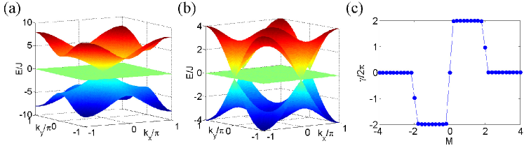
Figure 31: (Color online) The energy spectra and topological features of the 2D Maxwell lattices [355]. (a) The energy spectrum for $M=2$; (b) The energy spectrum for $M=0$; (c) The Berry phase $\gamma$ as a function of the parameter $M$, which corresponds to the Chern number $\mathcal{C}_{1}=\gamma/2\pi$ when the 2D system is in the insulating phase with $M\neq 0,\pm 2$. Reprinted with permission from Zhu et al.[355]. Copyright© (2017) by the American Physical Society.

The system is in an insulating state when $M\neq 0,\pm 2$ since there is a gap between any two of the three bands. Then one can calculate the corresponding Chern number $\mathcal{C}_{n}$ for the three bands:

$$C_{n}=\frac{1}{2\pi}\int_{BZ}{dk_{x}dk_{y}}F_{xy}(k_{x},k_{y})=\gamma/2\pi.$$ (171)

Here $n=-1,0,1$ label the band index corresponding to the lowest, middle, and highest band, respectively. Direct calculation indicates that nonzero Chern numbers $C_{-1}=-C_{1}=2\text{sgn}(M)$ for $|M|<2$ and $C_{-1}=C_{1}=0$ for $|M|>2$, and thus the zero Chern number $C_{0}(M)=0$ for the flat band. Figure 31(d) shows the phase diagrams of this model characterized by $\gamma/{2\pi}$ of the lowest band as a function of the parameter $M$, which implies topological phase transition with band closing in this system when $M=-2,0,2$. In addition, a correspondence between the helicity of these edge states and the polarization of photons was found by investigating the edge modes between the first gap. For the case $0<M<2$, the system is a non-trivial insulator with $C=2$. Under the open boundary condition along the $x$ direction, there are two edge states for each edge and the corresponding effective Hamiltonian is given by $\mathcal{H}_{\text{edge}}=v_{y}k_{y}\hat{S}_{y}.$ This edge Hamiltonian is the 1D Hamiltonian of circularly-polarized photons [355]. The helicity operator defined as

$$h=\hat{\mathbf{S}}\cdot{\mathbf{k}}/{|\mathbf{k}|}=\text{sgn}(k_{y})\hat{S}_{y}$$ (172)

is the projection of the spin along the direction of the linear momentum [351]. Hence, the edge quasiparticle-streams in this Maxwell topological insulator can be treated as Maxwell fermion-streams with the same helicities $h\equiv\langle\hat{h}\rangle=+1$ for opposite momenta.

The model Hamiltonian determined by the Bloch vector (167) can be generalized to the 3D model by adding an external term $-2J\text{cos}k_{z}$ to the $z$-component of ${\bf R}(\mathbf{k})$. Thus the Bloch Hamiltonian preserves inversion symmetry ($\hat{P}$) represented as $\hat{P}\mathcal{H}(\mathbf{k})\hat{P}^{-1}=\mathcal{H}(\mathbf{-k})$ and breaks the TRS ($\hat{T}$) since $\hat{T}\mathcal{H}(\mathbf{k})\hat{T}^{-1}\neq\mathcal{H}(-\mathbf{k}),$ where $\hat{P}=\text{diag}(1,1,-1)$ and $\hat{T}=\hat{I}\hat{\mathcal{K}}$, with $\hat{I}=\text{diag}(1,1,1)$ and $\hat{\mathcal{K}}$ being the complex conjugate operator. The system is a Maxwell metal for $|M|<3$ and a normal insulator for $|M|>3$. For simplicity, we consider the typical case of $M=2$, where the band spectrum hosts two Maxwell points in the first BZ at $\mathbf{M}_{\pm}=\begin{pmatrix}0,0,\pm\frac{\pi}{2}\end{pmatrix}$. The corresponding low-energy effective Hamiltonian now becomes

$$\mathcal{H}_{M_{\pm}}(\mathbf{q})=vq_{x}\hat{S}_{x}+vq_{y}\hat{S}_{y}\pm{vq_{z}\hat{S}_{z}}.$$ (173)

The two 3D Maxwell points have topological monopoles $\mathcal{C}_{M_{\pm}}=\pm 2$, which is defined in terms of a Chern number (defined by the lowest band) on a sphere enclosing the band touching point. There are two Fermi arcs connecting the two points under open boundary condition, which are similar to those in double-Weyl semimetals. The difference between them is that the 3D Maxwell points in Maxwell metals have linear momenta along all three directions, while the dispersion near double-Weyl points takes the quadratic form. Besides, the topological stability of Maxwell points is weaker than that of Weyl points. In this proposed model, the band gaps will be opened and Maxwell points will disappear when the inversion symmetry is broken by introducing a perturbation term with one of the other five $SU(3)$ Gell-Mann matrices.

Two different schemes were proposed to realize the spin-1 Maxwell fermions in OLs [355]. The first scheme is to use non-interacting fermionic atoms in a square or cubic OL and choose three atomic internal states in the ground state manifold to encode the three spin states. Using three atomic internal states to form the pseudospin-1 basis leads to the realization of Maxwell fermions in a lattice of simplest geometry, i.e., a primitive square or cubic lattice. Moreover, Maxwell fermions can be alternatively realized by using single-component fermionic atoms in OLs with three sublattices, where the pseudospin-1 basis is represented by the three sublattices in a unit cell. Both schemes involve Raman-assisted hopping with proper laser-frequency and polarization selections [355], which is similar to the method we discussed in Sec. 4.3.5.

Inspired by the investigation of type-II Weyl semimetals, a recent work studied the topological triply-degenerate points [360] in OLs induced by spin-tensor-momentum coupling [358]. These triply-degenerate points possess fermionic excitations with effective integer spins. As we mentioned above, a 3D Maxwell point with threefold degeneracy will be destroyed by a small spin-tensor perturbation $\thicksim N_{ij}$. Here the spin-1 matrices $\hat{\bf S}$ are also termed spin-vector-momentum-coupling, and the spin-tensor-coupling matrices $N_{ij}=(\hat{S}_{i}\hat{S}_{j}+\hat{S}_{j}\hat{S}_{i})/2$ $(i,j=x,y,z)$ are equivalent to the so-called Gell-Mann matrices, which form a basis of the $SU(3)$ algebra. A simple Hamiltonian of a stable triply-degenerate point induced by a momentum-dependent term $k_{i}N_{ij}$ is as follows [358]

$$\mathcal{H}(\mathbf{k})=k_{x}\hat{S}_{x}+k_{y}\hat{S}_{y}+k_{z}(\alpha\hat{S}_{z}+\beta N_{ij}),$$ (174)

where the spin-tensor $N_{ij}$ is coupled to the $k_{z}$ direction. At $k=0$, $\mathcal{H}(k)$ exhibits a triply-degenerate point with a topological charge $C$. The model Hamiltonian (174) has a symmetry $\mathcal{H}(\mathbf{k})=-\mathcal{H}(-\mathbf{k})$, indicating that the Chern number $C_{1}=-C_{-1}$ for the upper and lower bands and $C_{0}=0$ for the middle one. For convenience, we use the lower-band Chern number as an topological invariant for labeling triply-degenerate points, i.e., $C=C_{-1}$. For $\beta=0$, such a triply-degenerate point is the 3D Maxwell point we discussed before, which carries the topological monopole

$$C=\frac{1}{2\pi}\oint_{\mathcal{S}}\mathbf{F}_{-}(\mathbf{k})\cdot d\mathcal{S}=2\text{sgn}(\alpha),$$ (175)

where $\mathcal{S}$ is a surface enclosing a triply-degenerate point, and $\mathbf{F}_{-}(\mathbf{k})=\nabla\times\langle{u_{-}(\mathbf{k})|i\partial_{\mathbf{k}}|u_{-}(\mathbf{k})\rangle}=\text{sgn}(\alpha)\mathbf{k}/|\mathbf{k}|^{3}$. Hereafter, the simplest triply-degenerate point with topological monopoles ${C}=\pm 2$ is named type-I triply-degenerate point. In addition, a nonzero $\beta N_{ij}$ term will induce three types of triply-degenerate points [358] in Eq. (174). The monopole charge of a type-I triply-degenerate point will not be changed by the three spin-tensors $N_{xx}$, $N_{yy}$, and $N_{xy}$. The tensor $N_{zz}$ induces a type-II triply-degenerate point with $C=\pm 1$ for $|\beta|>|\alpha|\neq 0$. A type-III triply-degenerate point with $C=0$ can be induced by the tensor $N_{xz}$ or $N_{yz}$ for $|\beta|>2|\alpha|\neq 0$.

It was proposed to realize type-II and type-III triply-degenerate points by coupling three atomic hyperfine states, based on the realization of spin-tensor-momentum coupling and spin-vector-momentum-coupling with spin-1 cold atoms [362, 363, 260, 364]. The realization of topological monopoles of three different types of triply-degenerate points and investigation of their geometric properties using the parameter space formed by three hyperfine states of ultracold atoms coupled by radio-frequency fields was proposed [361]. The Maxwell points has recently been experimentally realized in the parameter space of a superconducting qutrit [357], where the other two types of triply-degenerate points may also be realized in this artificial atom system. Furthermore, there is potential to study even higher spin qusiparticles with untracold atoms. For instance, the spin-3/2 qusiparticles satisfy the so-called Rarita-Schwinger equation in Rarita-Schwinger-Weyl semimetal [352], and Dirac-Weyl fermions with arbitrary spin in 2D optical superlattices [351].

5 Probing methods

Since the atoms are neutral, the traditional transport measurements in solids that can be used to determine the topological bands, such as measuring the Chern numbers via the QHE, are very challenging in cold atomic systems. Therefore, new methods of probing the topological states of matter in cold atom systems are needed. On the other hand, some topological invariants, such as the underlying Berry curvature as the central measure of topology, could be directly measured in OL systems, which is not easily accessible in traditional condensed matter materials. In this section, we review the methods developed to reveal intrinsic properties of topological states and phenomena in cold atom systems. We focus our discussion on the noninteracting atomic gases in OLs, highlighting those experimental probes of topological invariants that are specific to the single-particle topological Bloch bands, and will mention extensions to the topological atomic states with interactions.

5.1 Detection of Dirac points and topological transition

It has been demonstrated that the Dirac points (massless Dirac fermions) in a honeycomb OL can be probed from measuring the atomic fraction tunnelling to the upper band in Bloch oscillations [77, 216, 215], which is the Landau-Zener transitions between the two energy bands. The starting point of the experiment is a ultracold gas of fermionic ⁴⁰K prepared in the lowest-energy band of a honeycomb OL. The atomic cloud is then subjected to a constant force $F$ along the $x$ direction by application of a weak magnetic field gradient, as the effect is equivalent to that produced by an electric field in solid-state systems. As shown in Fig. 32, the atoms are accelerated such that their quasi-momentum $q_{x}$ increases linearly up to the edge of the BZ, where a Bragg reflection occurs. The cloud eventually returns to the centre of the band, performing one full Bloch oscillation, and the quasi-momentum distribution of the atoms in the different bands is measured. For a trajectory far from the Dirac points, the atoms remain in the lowest-energy band. In contrast, when passing through a Dirac point, the atoms are transferred from the first band to the second because of the vanishing energy splitting at the linear band crossing. Thus, the points (position) of maximum transfer factions can be used to identify the Dirac points as the transition probability in a single Landau-Zener event increases exponentially as the energy gap decreases. Moreover, the topological transition from gapless (massless Dirac fermions) to gapped bands (massive Dirac fermions) can also be mapped out by recording the fraction of atoms transferred to the second band. This Bloch-Landau-Zener-oscillation technique can be extended to detect other band-touching points, such as the Weyl points and nodal lines in 3D OLs [365, 258, 275, 285].

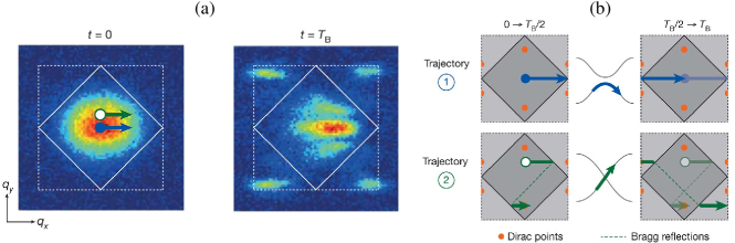
Figure 32: (Color online) Detecting Dirac points from Bloch-Landau-Zener transition. (a) The quasi-momentum distribution of the atoms before and after one Bloch oscillation, and (b) the corresponding trajectories. Reprinted by permission from Macmillan Publishers Ltd: Tarruell et al.[77], copyright© (2012).

The Bragg spectroscopy can provide an alternative method to confirm the linear dispersion relation for the massless Dirac fermions and the energy gap for the massive ones [76]. As shown in Fig. 33(a), two laser beams are shined on the atomic gas in the Bragg spectroscopy, by fixing the angle between the two beams, which gives rise to the relative momentum transfer $\mathbf{q=k}_{2}-\mathbf{k}_{1}$, with $\mathbf{k}_{i}$ being the wave vector of each laser beam. One can then measure the atomic transition rate by scanning the laser frequency difference $\omega=\omega_{2}-\omega_{1}$. From the Fermi’s golden rule, this transition rate basically measures the following dynamical structure factor

$$S(\mathbf{q},\omega)=\sum_{\mathbf{k}_{1},\mathbf{k}_{2}}|\langle f_{\mathbf{k}_{2}}|H_{B}|i_{\mathbf{k}_{1}}\rangle|^{2}\delta[\hbar\omega-E_{f\mathbf{k}_{2}}+E_{i\mathbf{k}_{1}}],$$ (176)

where $H_{B}=\sum_{\mathbf{k}_{1},\mathbf{k}_{2}}\Omega e^{i\mathbf{q\cdot r}}|i_{\mathbf{k}_{1}}\rangle\langle f_{\mathbf{k}_{2}}|+h.c.$ is the light-atom interaction Hamiltonian, and $|i_{\mathbf{k}_{1}}\rangle$ and $|f_{\mathbf{k}_{2}}\rangle$ denote the initial and the final atomic states with the energies $E_{i\mathbf{k}_{1}}$ and $E_{f\mathbf{k}_{2}}$ and the momenta $\mathbf{k}_{1}$ and $\mathbf{k}_{2}$, respectively. At the half filling, the excitations are dominantly around the Dirac point, and $S(q,\omega)$ has the expression for the massless Dirac fermions [76]

$$S(q,\omega)=\left\{\begin{array}[]{ll}0,&\hbox{$\omega\leqslant\omega_{r}$;}\\ \frac{\pi\Omega^{2}}{8v_{F}}\frac{2q_{r}^{2}-q^{2}}{\sqrt{q_{r}^{2}-q^{2}}}\Upsilon(\omega-\omega_{r}),&\hbox{$\omega>\omega_{r}$.}\end{array}\right.$$ (177)

where $\Upsilon$ is the unit step function, $\omega_{r}=qv_{F}/\hbar$ ($q\equiv\left|\mathbf{q}\right|$) and $q_{r}=\hbar\omega/v_{F}$. For massive Dirac fermions with the dispersion $E\approx\pm(\Delta_{g}+\hbar^{2}q_{x}^{2}/2m_{x}+\hbar^{2}q_{y}^{2}/2m_{y})$ with the effective mass $m_{x,y}=\hbar^{2}\Delta_{g}/v_{{}_{x},_{y}}^{2}$, the Fermi velocity $q_{x,y}$ along $x,y$ axis and the energy gap $\Delta_{g}$, the dynamical structure factor becomes [76]

$$S(q,\omega)=\left\{\begin{array}[]{ll}0,&\hbox{$\omega\leqslant\omega_{r}$;}\\ \frac{\pi\Omega^{2}\Delta_{g}}{2v_{{}_{x}}v_{{}_{y}}}\Upsilon(\omega-\omega_{c}^{x,y}),&\hbox{$\omega>\omega_{r}$.}\end{array}\right.$$ (178)

where $\omega_{c}^{x,y}=2\Delta_{g}+\hbar^{2}q_{x,y}^{2}/4m_{x,y}$. As shown in Fig. 33(b), the dynamical structure factor for massless Dirac fermions has the lower cutoff frequency $\omega_{r}$ that is linearly proportional to the momentum difference $q$ and vanishes when $q$ tends to zero. For massive ones, the lower cutoff frequency $\omega_{c}^{x,y}$ does not vanish as the momentum transfer goes to zero. This distinctive difference between the dynamical structure factors can be used to distinguish the cases with massive or massless Dirac fermions. Similar Bragg-spectroscopy methods were proposed to probe the edge and bulk states in 2D Chern insulators in OLs [366, 203, 234, 367], such that the topological phase transition from trivial insulating phase to quantum anomalous Hall phase can be detected.

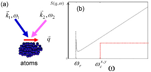
Figure 33: (Color online) Detecting Dirac fermions from Bragg spectroscopy [76]. (a) Schematic of the Bragg scattering. (b) The dynamic structure factors $S(\mathbf{q},\omega)$ for the massless Dirac fermions (solid line) and for the massive ones (dotted line).

5.2 Interferometer in momentum space

An interferometric method for measuring Berry’s phases and topological properties of Bloch bands for ultracold atoms in 2D OLs was proposed in Ref.[368]. The proposal is based on a combination of Ramsey interference and Bloch oscillations in the BZ to measure Zak phases, which can be used to measure $\pi$ Berry’s phase of Dirac points and the first Chern number of topological bands.

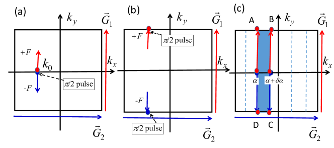
Figure 34: (Color online) An interferometer method to measure the Zak phase and Chern number [368]. A cloud of ultracold atoms with a well-defined quasi-momentum ${\bf k_{0}}$ in the spin-up state is initially loaded into a 2D OL, with ${\bf G_{1}}$ and ${\bf G_{2}}$ as reciprocal lattice vectors. (a) A $\pi/2$ pulse creates a coherent superposition of $|\!\!\uparrow\rangle$ and $|\!\!\downarrow\rangle$ states. Then spin-selective forces $\pm{\bf F}$ parallel to ${\bf G_{1}}$ are applied. (b) The two spins meet in the quasi-momentum space after half a period of Bloch oscillations, following by another $\pi/2$ pulse. The accumulated phase difference between the two states containing the Zak phase is measured from the resulting Ramsey fringe. (c) The Chern number of the band can be measured from the Zak phase across the primitive cell.

The scheme for measuring the Zak phase consists of three steps, as shown in Figs. 34 (a,b). The atoms are initially prepared in a spin-up state with a given quasi-momentum ${\bf k_{0}}$ in the $n$th band, and a first $\pi/2$ pulse is used to create a coherent superposition of two spin states denoted by the wave function $\psi_{{\bf k_{0}}n}({\bf r})\otimes({|\uparrow\rangle+|\downarrow\rangle})/{\sqrt{2}}$. The eigenfunctions in the $n$th band is written as $\psi_{{\bf k}n}({\bf r})=e^{i{\bf kr}}u_{{\bf k}n}({\bf r})$, where $u_{{\bf k}n}$ is the cell-periodic Bloch function, satisfying $u_{{\bf k}n}({\bf r+G_{i}})=u_{{\bf k}n}({\bf r})$ with two primitive reciprocal lattice vectors ${\bf G_{i}}$ ($i=1,2$). Next, opposite forces $\pm{\bf F}$ on the spin-up and spin-down are applied parallel to some reciprocal lattice vector ${\bf G_{1}}$, which can be created by a magnetic field gradient along the $y$ axis. The atoms then exhibit the Bloch oscillations in the momentum space, which is assumed to be adiabatic. In this case, the evolution under the application of the force $\pm{\bf F}$ is described by the time-dependent wave function $(\Psi_{\uparrow}({\bf r,t})\otimes{|\uparrow\rangle}+\Psi_{\downarrow}({\bf r,t})\otimes{|\downarrow\rangle})/{\sqrt{2}}$. The wave functions $\Psi_{\sigma}({\bf r,t})$ ($\sigma=\uparrow,\downarrow$) obey the Schrödinger equation $i\hbar{\partial\Psi_{\sigma}({\bf r},t)}/{\partial t}=H_{\sigma}\Psi_{\sigma}({\bf r,t}),$ where the Hamiltonian

$$H_{\uparrow,\downarrow}=H_{0}\mp{\bf F}{\bf r}\pm E_{Z},\,\,H_{0}=-\frac{\hbar^{2}}{2m}\nabla^{2}+V({\bf r}),$$ (179)

with $V({\bf r})$ being the lattice potential and $E_{Z}$ being the Zeeman energy. Under the adiabatic condition, the atoms remain within the Bloch band. The wave functions take the form: $\Psi_{\uparrow(\downarrow)}({\bf r,t})=e^{i\xi_{\uparrow(\downarrow)}(t)}\psi_{{\bf k_{\pm}(t)},n}({\bf r}),$ where ${\bf k_{\pm}}(t)={\bf k_{0}}\pm{\bf f}t$, ${\bf f}={\bf F}/\hbar$, and the phase $\xi_{\uparrow(\downarrow)}(t)$ is given by:

$$\xi_{\uparrow(\downarrow)}(t)=i\int_{\bf k_{0}}^{{\bf k_{\pm}}(t)}\langle u_{{\bf k^{\prime}}n}|\nabla_{\bf k^{\prime}}u_{{\bf k^{\prime}}n}\rangle d{\bf k^{\prime}}-\frac{1}{\hbar}\int_{0}^{t}\epsilon_{n}({\bf k_{\pm}}(t^{\prime}))dt^{\prime}\mp\frac{E_{Z}t}{\hbar}.$$ (180)

After half a period of the Bloch oscillations (period is given by $T=|\bf{G}_{1}|/|{\bf f}|$), the two spins meet at the edge of the first BZ, another $\pi/2$ pulse is applied to perform the Ramsey interferometry, which measures the phase difference picked up by the two spin species $\xi_{\uparrow}(T/2)-\xi_{\downarrow}(T/2)$. During such an evolution, the up and down states pick up the geometric Zak phase, which can be determined from the Ramsey phase:

$$\varphi_{\rm tot}=\varphi_{\rm Zak}+\varphi_{\rm dyn}+\varphi_{\rm Zeeman},$$ (181)

where the Zak phase is given by:

$$\varphi_{\rm Zak}=i\int_{{\bf k_{0}-G}/2}^{{\bf k_{0}+G}/2}\langle u_{{\bf k^{\prime}}n}|\nabla_{\bf k^{\prime}}u_{{\bf k^{\prime}}n}\rangle d{\bf k^{\prime}}$$ (182)

and the dynamical phase and Zeeman phase are given by $\varphi_{\rm dyn}=-\frac{1}{\hbar}\int_{-T/2}^{T/2}{\rm sgn}(t^{\prime})\epsilon_{n}({\bf k_{0}}+{\bf f}t^{\prime})dt^{\prime}$ and $\varphi_{\rm Zeeman}=-{E_{Z}T}/{\hbar}$, respectively. For a band structure with symmetric dispersion relation, $\epsilon_{n}({\bf k_{0}+{\bf f}}t^{\prime})=\epsilon_{n}({\bf k_{0}-{\bf f}}t^{\prime})$, the dynamical phase vanishes. The Zeeman phase can be also eliminated by a spin echo sequence [368, 125]. Thus, the Ramsey interferometry can directly give the Zak phase.

The interferometer scheme can be further used to measure the Chern number of a gapped band for cold atoms in 2D OLs. As shown in Fig. 34 (c), the initial quasi-momentum can be prepared to ${\bf k}(\alpha)=\alpha{\bf G_{2}}$, where $\alpha\in[0;1)$. Then the Zak phase for a specific $\alpha$ can be measured through the interferometer protocol. The small change of Zak phase as $\alpha$ is increased by $\delta\alpha$ is equal to the integral of the Berry curvature over the rectangle $\delta S$ defined by the corresponding trajectories, which is the Berry’s phase for the contour $ABCDA$. To see this, one can choose a smooth gauge for the periodic Bloch function in $\delta S$, such that the Berry’s phase $\gamma$ can be represented as the sum of the Berry’s phases for the four sides of the rectangle, $\gamma=\gamma_{AB}+\gamma_{BC}+\gamma_{CD}+\gamma_{DA}$. Since the sides $AB$ and $CD$ are equivalent but traversed in the opposite direction, their contribution vanishes, $\gamma_{AB}+\gamma_{CD}=0$, then $\gamma_{BC}+\gamma_{DA}$ is equal to the difference of the Zak phases for trajectories $BC$ and $DA$. Thus, the change of the Zak phase is related to the Berry phase and is given by an integral of the Berry curvature:

$$\gamma=\int_{\delta{\cal S}}d^{2}k\Omega({\bf k})=-ie^{-i\varphi_{\rm Zak}(\alpha)}\partial_{\alpha}e^{i\varphi_{\rm Zak}(\alpha)}\delta\alpha.$$ (183)

As the Chern number $C=\frac{1}{2\pi}\int_{\rm BZ}d^{2}k\Omega({\bf k})$, we then obtain $C$ from the winding number of the Zak phase [131],

$$C=-\frac{i}{2\pi}\int_{0}^{1}d\alpha e^{-i\varphi_{\rm Zak}(\alpha)}\partial_{\alpha}e^{i\varphi_{\rm Zak}(\alpha)}.$$ (184)

This relation implies that the Chern number can be extracted from the interferometric measurements of the Zak phase across the BZ. The method for a more general lattice structure is introduced in Ref. [368]. In addition, the $\pi$ Berry phase of a Dirac point can also be determined from the interferometric measurement over a trajectory enclosing the point in the momentum space.

The proposed interferometer method has been demonstrated in cold atom experiments [125, 140]. The Zak phase of topological Bloch bands for cold atoms in a 1D dimerized OL, which realizes the SSH/Rice-Mele Hamiltonians (see Sec. 4.1.1), has been directly detected from the interferometric measurements [125]. Furthermore, the atomic interferometer to measure $\pi$ Berry flux of a Dirac point in momentum space has also been demonstrated [140], which is in analogy to an Aharonov-Bohm interferometer that measures magnetic flux in real space (See Sec. 4.2.1).

Based on the proposed measurements of non-Abelian generalizations of Zak phases (the Wilson loops) or time-reversal polarizations, the interferometric method by combining the Bloch oscillations with Ramsey interferometry can be generalized to probe $\mathbb{Z}_{2}$ topological invariants of time-reversal-invariant topological insulators realized in OLs [369]. Moreover, by using an additional mobile impurities that bind to quasiparticles of a host many-body system, an interferometric scheme for detecting many-body topological invariants of interacting states with topological order, such as the fractional excitations in fractional quantum Hall systems, was proposed in Ref. [370].

5.3 Hall drift of accelerated wave packets

For a wavepacket evolving on a lattice, which is centered at position $\boldsymbol{r}$ with the quasimomentum $\boldsymbol{k}$ and driven by an external force $\boldsymbol{F}$, the equations of motion are given by [131]

$$\dot{\boldsymbol{r}}_{n}=\frac{1}{\hbar}\frac{\partial E_{n}(\boldsymbol{k})}{\partial\boldsymbol{k}}-(\dot{\boldsymbol{k}}\times\boldsymbol{e}_{z})\Omega_{n}(\boldsymbol{k}),\leavevmode\nobreak\ \leavevmode\nobreak\ \hbar\dot{\boldsymbol{k}}=\boldsymbol{F},$$ (185)

where $\Omega_{n}(\boldsymbol{k})$ is the Berry’s curvature of the $n$-band, and $E_{n}(\boldsymbol{k})$ is the corresponding band structure. Here the equations are valid when the force $\boldsymbol{F}$ is weak enough to preclude any inter-band transitions. Considering a 2D lattice and the force along the $y$ direction $\boldsymbol{F}=F\boldsymbol{e}_{y}$, the average velocity $\boldsymbol{v}_{n}=\dot{\boldsymbol{r}}_{n}$ along the transverse ($x$) direction can be obtained as

$$v_{n}^{x}(\boldsymbol{k})=\frac{\partial E_{n}(\boldsymbol{k})}{\hbar\partial k_{x}}-\frac{F}{\hbar}\Omega_{n}(\boldsymbol{k}).$$ (186)

The first term in the above equation describes the usual band velocity for Bloch oscillations, and the second term related to the Berry curvature is the so-called anomalous velocity, which can produce a net drift transverse to the applied force. It was shown that the anomalous velocity can be isolated and observed by canceling the contribution from the band velocity through comparing trajectories for opposite forces $\pm F$ [371]. Following this protocol, a measurement of the averaged velocity of the accelerated wavepacket for many trajectories gives the Berry’s curvature $\Omega_{n}(\boldsymbol{k})$ over a “pixelated” BZ, and thus the Chern number can be evaluated by properly adjusting the paths. In the experiment of realizing the Haldane model with ultracold fermions [28], the drift measurement has been performed to probe the nontrivial Berry curvature and map out the topological regime of the model (see Sec. 4.2.3 ).

It was further shown that the Chern number could be directly measured by imaging the center-of-mass drift of a Fermi gas as an effective Hall response to the external force [372]. Due to the periodicity of the energies in $k$-space,

$$\int_{\mathrm{BZ}}\bigl{(}\partial E_{n}(\boldsymbol{k})/\partial k_{x}\bigr{)}\,d^{2}k=0,$$ (187)

so the contribution from the band velocity naturally vanishes by averaging the velocity over the entire first BZ. By setting the Fermi energy within a topological bulk gap, the averaged anomalous velocity can thus be isolated by uniformly populating the bands, and the displacement along the transverse direction is directly proportional to the Chern number [372, 344]. Considering a general square lattice system of size $A_{\mathrm{syst}}\!=\!L_{x}\!\times\!L_{y}$ and a unit cell size $A_{\mathrm{cell}}$, the number of states within each band is $N_{\mathrm{states}}\!=\!A_{\mathrm{syst}}/A_{\mathrm{cell}}$, and the total number of particles is $N_{\mathrm{tot}}=\sum_{n}N^{(n)}$, where $N^{(n)}$ is the number of particles occupying the $n$-band. By assuming that each band is populated homogeneously, the average number of particles in a Bloch state $u_{n}(\boldsymbol{k})$ is uniform over the BZ and is given by

$$\rho^{(n)}(\boldsymbol{k})=\rho^{(n)}=N^{(n)}/N_{\mathrm{states}},$$ (188)

which acts as the band filling factor. The total averaged velocity along the direction transverse to the force is given by [372]

$$v^{x}_{\mathrm{tot}}=-({FA_{\mathrm{cell}}}/{h})\sum_{n}N^{(n)}\,C^{(n)},$$ (189)

where $C^{(n)}=\frac{1}{2\pi}\sum_{\boldsymbol{k}}\Omega_{n}(\boldsymbol{k})\,\Delta k_{x}\Delta k_{y}\approx\frac{1}{2\pi}\int_{\mathrm{BZ}}\Omega_{n}(\boldsymbol{k})\,d^{2}k$ is the band Chern number, with $\Delta k_{x,y}=2\pi/L_{x,y}$. This equation reveals that the averaged transverse velocity of the wave packet is related to the Chern number, which is a topological invariant and remains a constant as long as the spectral gaps to other bands do not vanish. For a free spin-polarized Fermi gas at zero temperature loaded in a 2D OL with topological bands, the Fermi energy $E_{\mathrm{F}}$ within a spectral gap naturally leads to a perfect filling of the bands located below the gap with $\rho^{(n)}=N^{(n)}/N_{\mathrm{states}}=1$ for $E_{n}<E_{\mathrm{F}}$. Thus one has

$$v^{x}_{\mathrm{tot}}=-({FA_{\mathrm{syst}}}/{h})\sum_{E_{n}\!<\!E_{\mathrm{F}}}C^{(n)},$$ (190)

which indicates that the total velocity of the Fermi gas is directly related to the sum of Chern numbers associated with populated bands.

In cold atom experiments, one can also prepare a thermal Bose gas filling certain Bloch bands, such as the lowest band, to measure such a Hall (transverse) response [48]. If only the lowest band is filled, its Chern number $C$ can be simply extracted from the center-of-mass displacement of the Bose gas, as the transverse velocity of the center-of-mass is given by

$$v^{x}_{\mathrm{cm}}=v^{x}_{\mathrm{tot}}/N_{\mathrm{tot}}=-({FA_{\mathrm{cell}}}/{h})C.$$ (191)

Since both the unit cell area $A_{\mathrm{cell}}$ and the strength of the applied force $F$ can be precisely determined, the center-of-mass Hall drift $\Delta x_{\mathrm{cm}}(t)=v^{x}_{\mathrm{cm}}t$ offers a direct measure of the Chern number of the lowest band. This protocol of measuring Chern numbers was successfully implemented with bosonic atoms in artificially generated Hofstadter bands [48] (See Sec. 4.2.2). This simple scheme is robust against perturbations and could be applied to any cold-atom setups characterized by nontrivial Chern numbers. Moreover, this method could be extended to detect the $\mathbb{Z}_{2}$ topological states, where the spin Chern number could be deduced by subtracting the center-of-mass drifts associated with the two spin species.

5.4 Streda formula and density profiles

It was revealed by Strěda that the Hall conductivity and thus the first Chern number can be represented as the number of occupied states in the QHE [373]. Considering the Hofstadter model [218] on a 2D lattice subjected to a uniform magnetic field $B$ with the butterfly energy spectrum shown in Fig. 17, when the magnetic flux per plaquette is rational $\Phi=p/q$, this spectrum splits into $q$ sub-bands $E_{n}$ ($n=1,\dots,q$). Each bulk band $E_{n}(\boldsymbol{k})$ is associated with a Chern number $C^{(n)}$, which remains constant as long as the bulk gaps do not close. The quantized Hall conductivity of a 2D electron system can be obtained from the Strěda formula (let $h=c=e=1$)[373]:

$$\sigma_{H}=\sigma_{0}C=\sigma_{0}\sum_{E_{n}<E_{F}}C^{(n)}=\frac{\partial N(E)}{\partial B}\mid_{E=E_{F}}$$ (192)

where $\sigma_{0}$ is the conductivity quantum, the Chern number $C$ includes the contribution of all occupied bulk bands $C^{(n)}$, and $N$ is the number of states lying below the Fermi energy. The Strěda formula is valid when the Fermi energy $E_{F}$ lies in a gap.

For neutral atoms, by using the Strěda formula, it was proposed to extract the quantized Hall conductance and thus the Chern number from the measurement of atomic density profiles [229, 242]. For the OL with Fermi atoms, this quantized quantity is related to the particle density $\rho(r)$, which can be directly detected in practical experiments. For OL with a smooth confining potential $V_{c}(r)$, the spatial density profile $\rho(r)$ in the local-density approximation is

$$\rho(r)=\int dE\,D(E)\,\Theta[E_{F}-V_{c}(r)-E],$$ (193)

where $D(E)$ is the homogeneous-system density of states, and the density $\rho(r)$ actually counts the number of states below the “local chemical potential” $\mu(r)=E_{F}-V_{c}(r)$. When the local chemical potential lies in one of the gaps, we have $\partial\rho(r)/\partial\mu(r)=0$ because of vanishing compressibility, and thus the plateaus in the density profile appear, which correspond to the energy gaps in the energy spectrum [229]. The discernible number of plateaus is related to the size of the energy gaps. Generally, smaller gaps have higher values of Hall conductance, but it becomes increasingly harder to observe these gaps, as the corresponding plateaus will become discernible at lower temperatures and higher particle numbers. By comparing the density plateaus $\rho_{1,2}$ obtained from two different configurations of the magnetic flux $\Phi_{1,2}$ but corresponding to the opening of the same bulk gap in the bulk spectrum, one can obtain the analogue of the Strěda formula for the Hofstadter OL with the Chern number [229]:

$$C=\frac{\Delta\rho}{\Delta\Phi}=\frac{\rho_{2}-\rho_{1}}{\Phi_{2}-\Phi_{1}}=\sum_{n}C^{(n)}.$$ (194)

This equation is analogous to the quantized Hall conductivity of an electronic system with the Fermi energy set within the $n$th gap. In cold atom experiments, the Chern number can be extracted by comparing two measurements of atomic densities at different values of synthetic magnetic flux in the Hofstadter OL. Notably, it was shown in Ref. [232] that the Chern number could also be revealed in the momentum density $\rho(\boldsymbol{k})$ of the same Hofstadter OL.

A simple relation between the Chern number and the atomic density plateaus for the anomalous QHE in the Haldane model (see Sec. 4.2.3) was also obtained from the Strěda formula [242]. This density-profile-measurement method for probing the band topology has also been shown to be applicable in 1D OLs with non-interacting Fermi atoms [176] and interacting Bose atoms [189], as well as the chiral topological insulator in 3D OLs [309]. The intrinsic anomalous Hall effect in a Fermi gas loaded in a trap without OLs may be also observed through the response of atomic density to the synthetic magnetic field [112]. Thus, the measurement of the atom density plateaus with the analogous Strěda formula for cold atoms offers a general way to identify topological order and phase transitions [374, 208]. In practical experiments, one requires low temperature to make the atomic density plateaus visible, which is the main obstacle for demonstrating this detection method. For ⁴⁰K atoms in typical OLs, the plateaus will become visible when the temperature is lower than about 10 nK [229, 176].

5.5 Tomography of Bloch states

A method for full tomography of Bloch vectors was first proposed for a specific realization of a Haldane-Chern insulator in spin-dependent hexagonal OLs [244]. The Haldane model [13] and some other models of Chern insulators can be well described by two-band Bloch Hamiltonians of the form

$$\mathcal{H}(\boldsymbol{k})=\epsilon_{0}(\boldsymbol{k})\mathbf{I}_{2\times 2}+\boldsymbol{d}(\boldsymbol{k})\cdot\boldsymbol{\sigma},$$ (195)

with the Bloch vectors $\boldsymbol{d}(\boldsymbol{k})=d_{x,y,z}(\boldsymbol{k})$. The Berry curvature $\Omega$ and the Chern number $C$ of the lowest energy band can be expressed in terms of the normalized Bloch vector $\boldsymbol{n}(\boldsymbol{k})=\boldsymbol{d}(\boldsymbol{k})/|\boldsymbol{d}(\boldsymbol{k})|$ [64]:

$$\Omega(\boldsymbol{k})=\frac{1}{2}\boldsymbol{n}\cdot(\partial_{k_{x}}\boldsymbol{n}\times\partial_{k_{y}}\boldsymbol{n}),\ \ C=\frac{1}{2\pi}\int_{\text{BZ}}\Omega(\boldsymbol{k})d\boldsymbol{k}.$$ (196)

Based on this equation, when the system is in a phase $C\neq 0$, an experimental measurement of $\boldsymbol{n}(\boldsymbol{k})$ would depict a Skyrmion pattern on a “pixelated” BZ, leading to an approximate measurement of the Chern number. For a specific Haldane-like model that could be realized with fermionic atoms of two spin states confined on the two triangular sublattices of the honeycomb pattern, the Bloch vector distribution $\boldsymbol{n}(\boldsymbol{k})\propto\langle\boldsymbol{\sigma}\rangle$ can be experimentally determined from spin-resolved time-of-flight images [244]. In a typical experiment, after the ground state is prepared, switching off the trap in adequate timescales projects the atom cloud into the momentum density distributions $\rho_{a,b}(\boldsymbol{k})$, which give the pseudospin component $n_{z}(\boldsymbol{k})=\frac{1}{2}[\rho_{a}(\boldsymbol{k})-\rho_{b}(\boldsymbol{k})]/[\rho_{a}(\boldsymbol{k})+\rho_{b}(\mathbf{k})]$. A fast Raman pulse during time-of-flight allows one to rotate the atomic states and map $n_{x}$ and $n_{y}$, which is the tomography of the whole Bloch vector field. Actual experiments “pixelize” the time of flight images, counting the number of atoms on each “square” of the effective BZ and estimating the averages of $n_{x},\,n_{y}$ or $n_{z}$. Either through repetitions or through self-averaging in an experiment with multiple copies of the lattice, a set of normalized vectors $\{\mathbf{n}_{j}\}_{j=1}^{L\times L},$ evenly sampled over momentum space can be obtained, which gives the Chern number with the error $\mathcal{O}(4\pi^{2}/L^{2})$ expected from the discretization with the smooth integrand [244].

A different scheme for tomography of Bloch states in OLs with two sublattice states was further proposed, which is based on the quench dynamics and thus is not restricted to a specific system [375]. Consider spinless fermions in a 2D OL with two sublattice states $A$ and $B$, and the system is described by the two-band Hamiltonian in Eq. (195) with $\boldsymbol{\sigma}$ acting in the sublattice space. For every quasimomentum $\boldsymbol{k}$, the sublattice space defines a Bloch sphere, with north and south poles given by $|{\boldsymbol{k}}A\rangle$ and $|{\boldsymbol{k}}B\rangle$, respectively. The normalized vector on the Bloch sphere is parametrized as ${\boldsymbol{n}}(\boldsymbol{k})=(\text{sin}\vartheta_{\boldsymbol{k}}\text{cos}\varphi_{\boldsymbol{k}},\text{sin}\vartheta_{\boldsymbol{k}}\text{sin}\varphi_{\boldsymbol{k}},\text{cos}\vartheta_{\boldsymbol{k}})$. Then the Bloch state of the lowest band is given by $|\boldsymbol{k}-\rangle=\text{sin}(\vartheta_{\boldsymbol{k}}/2)|\boldsymbol{k}A\rangle-\text{cos}(\vartheta_{\boldsymbol{k}}/2)e^{i\varphi_{\boldsymbol{k}}}|\boldsymbol{k}B\rangle$. In order to obtain the full information of the Bloch state determined by $\vartheta_{\boldsymbol{k}}$ and $\varphi_{\boldsymbol{k}}$, one can measure the momentum distribution of the system, which is subjected to an abrupt quench with a potential off-set $\epsilon_{A}-\epsilon_{B}\equiv\hbar\omega_{AB}$ between $A$ and $B$ sites for suppressing tunneling at the measurement time $t_{m}$, leading to an observable dynamics in the momentum distribution [375]

$$\rho(\boldsymbol{k},t)=f(\boldsymbol{k})\{1-\text{sin}\vartheta_{\boldsymbol{k}}\text{cos}[\varphi_{\boldsymbol{k}}+\omega_{AB}(t-t_{m})]\}.$$ (197)

Here $f(\boldsymbol{k})$ is a broad envelope function given by the momentum distribution of the Wannier function. The oscillatory time dependence in $\rho(\boldsymbol{k},t)$ directly reveals both $\varphi_{\boldsymbol{k}}$ and $\text{sin}\vartheta_{\boldsymbol{k}}=1-|n_{z}(\boldsymbol{k})|^{2}$. The time-dependence of $\rho(\boldsymbol{k},t)$ allows one to reconstruct $n_{x,y,z}(\boldsymbol{k})$ from the amplitude and the phase of the oscillations. Such a complete tomography of the Bloch states is mandatory for a measurement of the Berry curvature. It was shown that this scheme is applicable to extract the Chern number and topological transitions for the Hofstadter model with $\pi$ flux and the Haldane model on a honeycomb OL [375].

An alternative but generic scheme for measuring the Bloch wavefunction based on the time-of-flight imaging was presented in Ref. [313]. For fermionic atoms with $N$ spin states referred as $|s\rangle$ ($s=1,2,...,N$) in a generic OL, the Bloch state in the non-degenerate $n$-band can be denoted by $|u_{n}(\mathbf{k})\rangle=\sum_{s=1}^{N}c_{ns}(\mathbf{k})|s\rangle$, where $c_{ns}(\mathbf{k})$ is the Bloch wavefunction with normalization $\sum_{s}|c_{ns}(\mathbf{k})|^{2}=1$. To measure $c_{ns}(\mathbf{k})$, one can first separate different spin components through a magnetic field gradient and directly map out the atomic momentum distribution $\rho_{ns}(\textbf{k})=|c_{ns}(\textbf{k})|^{2}$ for the filled band using the conventional time-of-flight imaging. One then measure the phase information of $c_{ns}(\textbf{k})$ by introducing a $\pi/2$ rotation between the two spin states denoted by $s$ and $s^{\prime}$ with an impulsive pulse light before the flight of atoms, which induces the transition

$$c_{ns}(\textbf{k})\rightarrow[c_{ns}(\textbf{k})+c_{ns^{\prime}}(\textbf{k})]/\sqrt{2},\ \ c_{ns^{\prime}}(\textbf{k})\rightarrow[c_{ns}(\textbf{k})-c_{ns^{\prime}}(\textbf{k})]/\sqrt{2}.$$

With this pulse, the difference between $|c_{ns}(\textbf{k})\pm c_{ns^{\prime}}(\textbf{k})|^{2}/2$ measured through time-of-flight imaging gives the real part of the interference terms $\text{Re}[c^{*}_{ns}(\textbf{k})c_{ns^{\prime}}(\textbf{k})]$. The imaginary part $\text{Im}[c^{*}_{ns}(\textbf{k})c_{ns^{\prime}}(\textbf{k})]$ can be obtained by the same way with a different rotation. The measurement of the population and interference terms determines the Bloch wave function up to an arbitrary overall phase $c_{ns}(\textbf{k})\rightarrow c_{ns}(\textbf{k})e^{i\chi(\textbf{k})}$, where $\chi(\textbf{k})$ in general depends on k instead of the spin index. This arbitrary $\mathbf{k}$-dependent phase poses an obstacle to measurement of the topological invariants, which can be overcame by a gauge-invariant method to calculate the Berry curvature based on the so-called $U(1)$-link defined for each pixel of the discrete BZ in experiments [376]. It was shown that the proposed method is generally applicable to probe the topological invariants in various topological bands [313, 265, 317] and robust to typical experimental imperfections such as inhomogeneous trapping potentials and disorders in the systems.

Recently, the tomography of Bloch states has been experimentally demonstrated with two different approaches [46, 45]. Based on the method proposed in Ref. [375], a full tomography of the Bloch states across the entire BZ was experimentally demonstrated by observing the quench dynamics at each momentum point [46]. In the experiment, a cloud of single-component fermionic ⁴⁰K atoms in a shaking hexagonal OL formed a tunable Floquet band insulator. Even though the global of the band has zero Chern number in the system, the measured distribution of Berry curvature showed the rich topology, such as the phase vortices as topological defects near Dirac points and their chiralities as the signal of the topological transition due to the shaking [46]. The topological defects of the Bloch states in the hexagonal OL were further experimentally studied by mapping out the azimuthal phase profile $\varphi_{\boldsymbol{k}}$ in the entire momentum space and by identifying the phase windings [377].

The state tomography methods discussed above are applicable for non-degenerate or isolated bands, where the Berry phase is merely a number. However, some lattice systems having multiple bands with degeneracies, such as in topological insulators and graphene, can seldom be understood with standard Berry phases but can instead be described using matrix-valued Wilson lines [378, 379, 369, 109]. Wilson lines as non-Abelian generalization of Berry phase [109] provide indispensable information to identify the topological structure of bands as they encode the geometry of degenerate states, such as the eigenvalues of Wilson-Zak loops (i.e., Wilson lines closed by a reciprocal lattice vector) for formulating the $Z_{2}$ topological invariants [378, 379, 369].

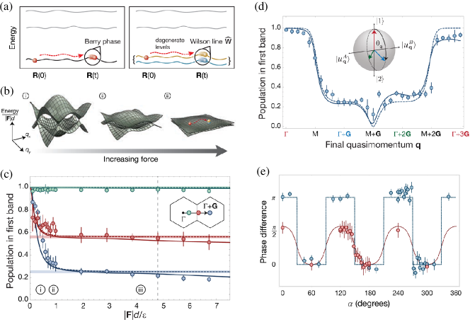
Figure 35: (Color online) Realizing the Wilson lines in the honeycomb lattice. (a) In a non-degenerate system (left), adiabatic evolution of a state through parameter space $\vec{R}$ results in the acquisition of a Berry phase. In a degenerate system (right), the evolution is instead governed by the matrix-valued Wilson line, which lead to population changes between the levels. (b) The band structure of the lowest two bands of the honeycomb lattice in effective energy units of $|\mathbf{F}|d$. As the force $\mathbf{F}$ is increased, the largest energy scale of the bands becomes small. At large forces (iii), the effect of the band energies is negligible and the system is effectively degenerate. In this regime, the evolution is governed by the Wilson line operator. (c) The measured population remaining in the first band for different forces after transport to $\Gamma+0.2\mathbf{G}$ (green), $\Gamma+0.55\mathbf{G}$ (red), and $\Gamma+\mathbf{G}$ (blue), where inset numbers i to iii refer to band schematics in (b). (d) Measuring mixing angles $\theta_{\mathbf{q}}$ at different final quasimomenta $\mathbf{q}$. (e) Measuring relative phases $\phi_{\mathbf{q}}$ at different $\mathbf{q}$, lying at angular coordinate $\alpha$ on a circle centered at $\Gamma$. The quantized jumps of $\pi$ in the phase of the interference fringe each time $\alpha$ is swept through a Dirac point. Reprinted from Li et al.[45]. Reprinted with permission from AAAS.

In a recent experiment [45], using an ultracold gas of rubidium atoms loaded in a honeycomb OL, the strong-force dynamics in Bloch bands that are described by Wilson lines was realized and an evolution in the band populations for revealing the band geometry was observed. This enables a full tomography of band eigenstates using Wilson lines. This approach can be used to determine the topological invariants in single- and multi-band systems. As shown in Fig. 35(a), the Berry phase merely multiplies a state by a phase factor, while the Wilson line is a matrix-valued operator that can mix state populations. The Wilson line was measured by detecting changes in the band populations under the influence of an external force $\mathbf{F}$, such that atoms with initial quasimomentum $\mathbf{q}(0)$ evolve to quasimomentum $\mathbf{q}(t)=\mathbf{q}(0)+\mathbf{F}t/\hbar$ after a time $t$. When the force is sufficiently weak and the bands are non-degenerate, the system will remain in the lowest band and the quantum state merely acquires a Berry phase and a dynamical phase. Transitions to other bands occur at stronger forces, and when the force is infinite with respect to a chosen set of bands, the effect of the dispersion vanishes and the bands appear as effectively degenerate, as shown in Fig. 35(b). The system then evolves according to the formalism for adiabatic motion in a degenerate system [109], and the dynamics is described by the unitary time-evolution operator as the Wilson line matrix [45]:

$$\hat{\mathbf{W}}_{\mathbf{q}(0)\rightarrow\mathbf{q}(t)}=\mathcal{\hat{P}}\text{exp}[i\int_{\mathcal{C}}d\mathbf{q}\hat{\mathbf{A}}_{\mathbf{q}}],$$ (198)

where the path-ordered $\mathcal{\hat{P}}$ integral runs over the path $\mathcal{C}$ in reciprocal space from $\mathbf{q}(0)$ to $\mathbf{q}(t)$ and $\mathbf{\hat{A}_{q}}$ is the Wilczek-Zee connection for local geometric properties of the state space. In the honeycomb OL, the Wilson line operator describing transport of a Bloch state from $\mathbf{Q}$ to $\mathbf{q}$ reduces to $\mathbf{\hat{W}}_{\mathbf{Q}\rightarrow\mathbf{q}}=e^{i(\mathbf{q}-\mathbf{Q})\cdot\hat{\mathbf{r}}}$, and thus the Wilson line operator simply measures the overlap between the cell-periodic Bloch functions denoted $|u_{\mathbf{Q}}^{n}\rangle$ and $|u_{\mathbf{q}}^{m}\rangle$ (with the band index $n,m$) at the initial and final quasimomenta [379]:

$$W^{mn}_{\mathbf{Q}\rightarrow\mathbf{q}}=\langle u_{\mathbf{q}}^{m}|u_{\mathbf{Q}}^{n}\rangle.$$ (199)

This enables a tomograph of the cell-periodic Bloch functions over the entire BZ in the basis of the states $|u_{\mathbf{Q}}^{n}\rangle$. In the experiment [45], a nearly pure BEC of ⁸⁷Rb was initially loaded into the lowest band at the center of the BZ $\mathbf{Q}=\Gamma$, and an inertial force, created by accelerating the lattice via linearly sweeping the frequency of the laser beams, was used to realize the Wilson line. The Wilson line was then verified by transporting the atoms from $\Gamma$ to different final quasimomenta using a variable force $|\mathbf{F}|$ and performing band mapping to measure the population remaining in the lowest band, as shown in Fig. 35(c). The saturation value $|W^{11}_{\Gamma\rightarrow\mathbf{q}}|^{2}=|\langle u_{\mathbf{q}}^{1}|u_{\Gamma}^{1}\rangle|^{2}$ of the population after transport to $\mathbf{q}$ is a measure of the overlap between the Bloch functions of the first band at $\Gamma$ and $\mathbf{q}$. To demonstrate the reconstruct of Bloch states using the Wilson lines, it is convenient to represent the state $|{u_{\mathbf{q}}^{1}}\rangle$ in the basis of $|1\rangle=|u_{\mathbf{Q}}^{1}\rangle$ and $|2\rangle=|u_{\mathbf{Q}}^{2}\rangle$ at a fixed reference quasimomentum $\mathbf{Q}$ as

$$|u_{\mathbf{q}}^{1}\rangle=\text{cos}\frac{\theta_{\mathbf{q}}}{2}|1\rangle+\text{sin}\frac{\theta_{\mathbf{q}}}{2}e^{i\phi_{\mathbf{q}}}|2\rangle.$$ (200)

Obtaining $\theta_{\mathbf{q}}$ and $\phi_{\mathbf{q}}$ for each quasimomentum $\mathbf{q}$ will map out the geometric structure of the lowest band [244, 375]. As shown in Fig. 35(d,e), mixing angles $\theta_{\mathbf{q}}$ at different final quasimomenta $\mathbf{q}$ was measured from the atom population remaining in the first band after the transport, and relative phases $\phi_{\mathbf{q}}$ at different $\mathbf{q}$ was measured through a procedure analogous to Ramsey or Stückelberg interferometry [45]. Using the data, the Bloch states in the lowest band $|u_{\mathbf{q}}^{1}\rangle$ and the eigenvalues of Wilson-Zak loops can both be reconstructed.

5.6 Spin polarization at high symmetry momenta

It was proposed that for a class of Chern insulators, the topological index can be obtained by only measuring the spin polarization of the atomic gas at highly symmetric points of the BZ [380]. The two-band Bloch Hamiltonian of the Chern insulators in square lattices is given by

$$\mathcal{H}(\mathbf{k})=[m_{z}-2J_{0}\text{cos}(k_{x}a)-2J_{0}\text{cos}(k_{y}a)]\sigma_{z}-2J_{\rm so}\text{sin}(k_{x}a)\sigma_{x}-2J_{\rm so}\text{sin}(k_{y}a)\sigma_{y},$$ (201)

where the $m_{z}$ is an effective Zeeman splitting, $J_{0}$ and $J_{\rm so}$ represent the nearest-neighbor spin-conserved and spin-flipped hopping coefficients, respectively. Notably, the cold-atom realization of this Hamiltonian with the needed 2D SOC has been theoretically proposed [117] and then experimentally achieved [36] by a simple optical Raman lattice scheme that applies two pairs of light beams to create the lattice and Raman potentials simultaneously. The topology of the lowest Bloch band can be characterized by the Chern number $C=\mbox{sgn}(m_{z})$ when $0<|m_{z}|<4J_{0}$, and otherwise $C=0$.

The lattice system has an inversion symmetry defined by the 2D inversion transformation $\hat{P}\otimes\hat{R}_{\rm 2D}$, where $\hat{P}=\sigma_{z}$ acting on spin space and $\hat{R}_{2D}$ transforms Bravais lattice vector $\mathbb{R}\rightarrow-\mathbb{R}$. For the corresponding Bloch Hamiltonian, one has $\hat{P}{\cal H}(\mathbb{k})\hat{P}^{-1}={\cal H}(-\mathbb{k})$, which follows that $[\hat{P},{\cal H}(\mathbb{\Lambda}_{i})]=0$ at the four highly symmetric points $\{\mathbb{\Lambda}_{i}\}=\{G(0,0),X_{1}(0,\pi),X_{2}(\pi,0),M(\pi,\pi)\}$. Therefore the Bloch states $|u_{\pm}(\mathbb{\Lambda}_{i})\rangle$ in the two energy bands are also eigenstates of the parity operator $\hat{P}$ with eigenvalues $P_{\pm}=+1$ or $-1$. The topology of the inversion-symmetric Chern band can also be determined by the following invariant [117, 36]

$$\Theta=\prod_{i}\text{sgn}[P_{-}(\mathbb{\Lambda}_{i})].$$ (202)

It can be proven rigorously that $\Theta=-1$ for the topological band, while $\Theta=1$ for the trivial band. Furthermore, for the square lattice with four highly symmetric points, the corresponding Chern number is given by $C=-\frac{1-\Theta}{4}\sum_{i=1}^{4}\text{sgn}[P(\mathbb{\Lambda}_{i})]$. Since the parity eigenstates are simply the spin eigenstates (here $\hat{P}=\sigma_{z}$), with the spin-up and spin-down corresponding to different atomic internal states, the topological invariants $\Theta$ and $C$ of the lowest Bloch band can be determined by measuring the spin polarization $P_{(-)}(\mathbf{k})$ of an atomic cloud at the four highly symmetric points:

$$P_{-}(\boldsymbol{\Lambda_{i}})=\frac{n_{\uparrow}(\boldsymbol{\Lambda_{i}})-n_{\downarrow}(\boldsymbol{\Lambda_{i}})}{n_{\uparrow}(\boldsymbol{\Lambda_{i}})+n_{\downarrow}(\boldsymbol{\Lambda_{i}})},$$ (203)

where $n_{\uparrow,\downarrow}(\boldsymbol{\Lambda_{i}})$ denotes the atomic momentum density of spin states $|\uparrow,\downarrow\rangle$, which can be measured directly by spin-resolved time-of-flight imaging. This method can be used to probe other topological bands with specific symmetries by measuring atomic spin polarization at highly symmetric points in momentum space, such as the chiral topological insulators [381, 165] and double-Weyl semimetals [275].

Based on the optical Raman lattice method [117], the Bloch Hamiltonian in Eq. (201) with the topological bands has been experimentally realized for a BEC of ⁸⁷Rb atoms [36]. For the condensate in the OL, the spin polarization at the four high symmetry momenta can be written as

$$\langle\sigma_{z}(\boldsymbol{\Lambda_{i}})\rangle\approx P_{-}(\boldsymbol{\Lambda_{i}})f(E_{-},T)+P_{+}(\boldsymbol{\Lambda_{i}})f(E_{+},T),$$ (204)

where $f(E_{\pm},T)=1/[e^{(E_{\pm}(\boldsymbol{\Lambda_{i}})-\mu)/k_{B}T}-1]$ is the BEC with $\mu$ and $T$ respectively being the chemical potential and temperature. Since $P_{+}(\boldsymbol{\Lambda_{i}})=-P_{-}(\boldsymbol{\Lambda_{i}})$, one has $\langle\sigma_{z}(\boldsymbol{\Lambda_{i}})\rangle\approx P_{-}(\boldsymbol{\Lambda_{i}})[f(E_{-},T)-f(E_{+},T)]$. Thus by preparing a cloud of bosonic atoms with the temperature satisfying $f(E_{-}(\boldsymbol{\Lambda_{i}}),T)>f(E_{+}(\boldsymbol{\Lambda_{i}}),T)$, one can obtain

$$\text{sgn}[\langle\sigma_{z}(\boldsymbol{\Lambda_{i}})\rangle]=\text{sgn}[P_{-}(\boldsymbol{\Lambda_{i}})].$$ (205)

Thus, the spin polarization can be precisely measured with a condensate at low temperature. In the experiment [36], the spin polarization was measured as a function of the tunable parameter $m_{z}$ to determine $\Theta$ and $C$ for the topology of the lowest-energy band, which is topologically nontrivial when $0<m_{z}<|m_{z}^{c}|$, whereas it is trivial for $m_{z}>|m_{z}^{c}|$, as show in Fig. 36. The 2D SOC and the band topology for BECs in the optical Raman lattices have recently been further investigated [260, 382, 383]

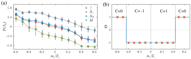
Figure 36: (Color online) (a) Measured spin polarization $P(\boldsymbol{\Lambda_{i}})$ at the four symmetric momenta $\boldsymbol{\Lambda_{i}}$ as a function of $m_{z}$. (b) Obtained invariant $\Theta$, which determines the Chern number $C$ of the lowest band in Hamiltonian (201). Reprinted from Wu et al.[36]. Reprinted with permission from AAAS.

5.7 Topological pumping approach

As introduced in Sec. 4.1.2, the topological pumping, geometric pumping, and spin pumping have been recently realized with ultracold atoms in 1D optical superlattices [157, 146, 158, 159]. Very recently, a 2D topological charge pump as a dynamical version of the 4D integer QHE was realized by using ultracold bosonic atoms in a 2D optical superlattice [17]. The quantized transported particle (i.e., the atomic center-of-mass change in the experiments) in the adiabatic cyclic evolution of these pumps indicates the underlying band topology, such as the first and second Chern numbers characterizing the 1D and 2D topological pumping, respectively.

Based on the pumping approach in OLs and hybrid Wannier functions in band theory [384], it was shown that the Chern number can be extracted from hybrid time-of-flight images [385]. In the modern theory of polarization, a 2D insulating lattice system can be viewed as a fictitious 1D insulator along one direction, say along $x$, subject to an external parameter $k_{y}$, where $k_{y}$ is the crystal-momentum along $y$. The polarization of this 1D insulator can be defined by means of hybrid Wannier functions [384], in which the Fourier transform from Bloch functions is carried out in the $y$ direction only. The polarization at each $k_{y}$ is then given by the center of the corresponding hybrid Wannier functions, and the change in polarization from adiabatically changing $k_{y}$ by $2\pi$ is proportional to the Chern number of the 2D insulators [384, 386]. This is a manifestation of topological particle pumping with $k_{y}$ being the adiabatic pumping parameter. A generalization of the hybrid Wannier functions of band theory to the hybrid particle densities in cold atomic gases $\rho(x,k_{y})$, which are the particle densities resolved along the $x$-direction as a function of $k_{y}$, provides a natural way to measure the Chern number in OLs. Experimentally, $\rho(x,k_{y})$ can be measured by combing in situ imaging along $x$ and time-of-flight imaging along the release direction $y$. In the measurement, the OL is switched off along the $y$ direction while the system remains unchanged in the $x$ direction. It was shown that the hybrid particle density provides an efficient numerical reconstruction of the Chern number in topologically-ordered OLs [385], such as the Hofstadter and Haldane models. This method is general and allows the measurement of other topological invariants in OLs, such as the $\mathbb{Z}_{2}$ topological invariant in time-reversal symmetric insulators and the $k_{z}$-dependent Chern number $C_{k_{z}}$ in Weyl semimetals [136, 275].

5.8 Detection of topological edge states

According to the bulk-edge correspondence, the topological index of the bulk bands corresponds to the number of gapless edge-modes present within the bulk gap [14, 15]. In Chern insulators, all the gapless edge states propagate in the same direction, such that they are chiral. In the context of the QHE, the chiral edge states are responsible for the quantized Hall conductivity. As introduced in Sec. 4.4, the chiral edge states in a quantum Hall ribbon have been experimentally realized and detected with cold atoms through the synthetic dimension method [37, 38]. In addition, the chiral currents were also observed in an optical ladder for ultracold bosonic atoms exposed to a uniform artificial magnetic field [174]. The high-resolution addressing technique in cold atom gases offers the possibility of directly visualizing the time-evolution of these edge states.

In a 2D atomic Chern insulator under an external trapping potential, the direct detection of topological edge states is challenging because the number of occupied edge modes within a bulk gap and below the Fermi level contains a very small fraction of the total number of particles. In addition, these edge states would be washed out by the smooth harmonic trap and thus one may not be able to distinguish them from the bulk states. To circumvent these problems in detecting the topological edge states, it was proposed to use a steep confining potential and to image the edge states from optical Bragg spectroscopy [366, 203, 234, 367]. Based on a generalization of Bragg spectroscopy sensitive to angular momentum [234], the Bragg probe can transfer energy and angular momentum to atoms located in the vicinity of the Fermi level and simultaneously changes their internal states, which completely removes the edge states from the cloud and allows imaging on a dark background unpolluted by the untransferred atoms. In this scheme, the Bragg spectra can provide an unambiguous signature of the topological edge states that establishes their chiral nature. Another method to directly image the propagating edge states was proposed by forcing them to propagate in a region that is unoccupied by the bulk states after suddenly removing the potential [235]. Other methods to visualize the edge state currents were also proposed by quenching the parameters of the system Hamiltonian [387, 388]. It would to interesting to extend these cold-atom schemes to directly image the helical edge states in $\mathbb{Z}_{2}$ topological insulators and the Fermi arc surface states in 3D topological semimetals.

6 Topological quantum matter in continuous form

In this section, we move beyond topological Bloch bands in lattice systems to describe some of the quantum matter in the continuum that have topologically nontrivial properties. Here we focus on there model systems realized with cold atoms without lattice potentials, which are the topological solitons in Jackiw-Rebbi model, various topological defects in BECs, and the atomic (quantum) spin Hall effect.

6.1 Jackiw-Rebbi model with topological solitons

In relativistic quantum field theory, Jackiw and Rebbi introduced a celebrated model to generate topological soliton modes with fractional particle numbers [124]. The Jackiw-Rebbi model describes a 1D Dirac field coupled to nontrivial background fields. The relativistic Dirac Hamiltonian for 1D Dirac fermions subjected to two static bosonic fields $\varphi_{1}$ and $\varphi_{2}$ can be written as [124, 127, 128]

$$H_{D}=c_{x}\sigma_{x}p_{x}+\varphi_{1}(x)\sigma_{z}+\varphi_{2}(x)\sigma_{y},$$ (206)

where $c_{x}$ is the (effective) speed of light and the background field with a kink potential can be described as

$$\varphi_{1}(x)=\Gamma,\leavevmode\nobreak\ \leavevmode\nobreak\ \varphi_{2}(x\rightarrow\pm\infty)=\pm\Delta_{0},$$ (207)

with positive constants $\Gamma$ and $\Delta_{0}$. The relativistic Dirac Hamiltonian with such a topologically nontrivial background potential supports an nondegenerate soliton state, which gives rise to fractionalization of particle number. In the original Jackiw-Rebbi model with $\Gamma=0$, the nondegenerate zero-energy soliton state is protected by the conjugation (particle-hole) symmetry that connects each state with energy $E$ to its partner located at the opposite energy. In the many-particle description, there are two degenerate many-body ground states corresponding to the soliton state being filled or empty, carrying fractional Fermi number $\mathcal{N}_{0}=\pm 1/2$, respectively.

Figure 37: (Color online) Fractionalization in Jackiw-Rebbi model [389]. (a) A background field with a pair of kink and anti-kink, both of which support a localized soliton state. (b) The energy spectrum and a pair of solitons with energies $E=\pm\Gamma$ and fractional particle numbers $\pm|\mathcal{N}_{0}|$. At the kink, the soliton state picks a fractional particle number of $|\mathcal{N}_{0}|$ from the effective valance band (Fermi sea) and another $1-|\mathcal{N}_{0}|$ from the effective conduction band, and vice versa for the opposite case at the anti-kink.

With the conjugation-symmetry-breaking term $\Gamma$, the soliton mode has non-zero energy and the particle number is generally irrational [127]:

$$\mathcal{N}_{0}=\frac{1}{\pi}\arctan\frac{\Delta_{0}}{\Gamma}.$$ (208)

One can see that $\mathcal{N}_{0}$ depends only on the asymptotic value of the kink rather than its detailed shape. In this sense, it is topological and is insensitive to local fluctuations of the background field. To have a better understanding of arbitrary fractional particle number [389], one can consider another kind of background field with a simple but practical configuration, that is, a pair of kink and anti-kink both with a step-function profile as shown in Fig. 37(a). Solving the energy spectrum of the Dirac Hamiltonian (206) at the kink potential (near $x=-a$) with $\varphi_{2}(x)=\Delta_{0}\text{sgn}(x+a)$ yields a localized in-gap eigenstate in the kink at $E=\Gamma$ with the wave function decaying as $\exp{(-\Delta_{0}|x+a|/\hbar c)}$ and the energy gap $E_{g}=2\sqrt{\Delta^{2}_{0}+\Gamma^{2}}$. It is understood that the soliton state picks up a fractional fermion number of $|\mathcal{N}_{0}|$ from the effective valance band (Fermi sea) and $(1-|\mathcal{N}_{0}|)$ from the effective conduction band, as shown in Fig. 37(b). Without the soliton, one can assume $N$ fermions fully occupying the valence band acting as a uniform background in the state counting. For filling with $N+1$ fermions in the presence of kink and anti-kink configuration, the expectation value of the fermion number of the soliton modes at the kink and anti-kink can be $|N_{0}|$ and $1-|N_{0}|$ if they are both occupied. For an anti-kink potential (near $x=a$) with $\varphi_{2}(x)=-\Delta_{0}\text{sgn}(x-a)$, the localized soliton state is obtained at $E=-\Gamma$ with the wave function decaying as $\exp{(-\Delta_{0}|x-a|/\hbar c_{x})}$. It picks up $(1-|\mathcal{N}_{0})|$ from the valence band and $|\mathcal{N}_{0}|$ from the conduction band. There must be pairs of kink and anti-kink in a periodic system. If both states are unoccupied, the particle numbers are $-|\mathcal{N}_{0}|$ at the kink and $|\mathcal{N}_{0}|-1$ at the anti-kink. When the Fermi level in this system, is tuned up, the $E=-\Gamma$ soliton state is occupied first and the particle numbers at kink and anti-kink are $\mp|\mathcal{N}_{0}|$, respectively. When both states are occupied, there are particles $(1-|\mathcal{N}_{0}|)$ and $|\mathcal{N}_{0}|$ at the kink and anti-kink, respectively.

The first condensed matter realization of the Jackiw-Rebbi model is the conducting polymers described by the SSH model for lattice systems, wherein the low-energy effective Hamiltonian of the Bloch Hamiltonian near Dirac points takes the Dirac form with kink-soliton modes in the continuum. In particular, the Jackiw-Rebbi model and the SSH model share many similar features related to topological insulators under a suitable regularisation. The soliton modes and related topological properties in the SSH model have been intensively investigated with cold atoms in 1D OLs (see Sec. 4.1.1).

The direct realization of the Jackiw-Rebbi model and the detection of the induced soliton mode with the fractional particle number by using a 1D atomic Fermi gas in the continuum were proposed in Ref. [389]. The first procedure is to create strong SOCs for the ultracold atoms, and the second one is to generate a kink-like potential and a tunable conjugation-symmetry-breaking term are properly constructed by laser-atom interactions, leading to an effective low-energy relativistic Dirac Hamiltonian with a topologically nontrivial background field. The fractionalization of the particle number in the atomic system may be detected through the soliton density and the local density of states near the kink by using two standard experimental detection methods for ultracold atomic gases, the in situ absorption imaging technique and spatially resolved rf spectroscopy [389]. The realization of 1D homogeneous Dirac-like Hamiltonian (particles) and related relativistic effects (e.g. Klein tunneling and Zitterbewegung) with cold atoms in the continuum has been studied in theories and experiments [92, 93, 95, 96, 390, 391, 105]. See Ref. [52] for a review on relativistic quantum effects of Dirac particles simulated by ultracold atoms.

6.2 Topological defects in Bose-Einstein condensates

BECs of atomic gases in a harmonic trap without lattice potentials can host various topological defects in real space. These topological defects include solitons in 1D, vortices and Skyrmions in 2D, monopoles, Skyrmions and knots in 3D. The topological defects have different physical properties and are classified by homotopy groups of their order-parameter space. Thus, they are distinguished by their topological charges with discrete values [392] and robust against to external perturbations. In particular, atomic BECs with internal spin degrees of freedom provide unique platforms for investigating different topological objects due to the rich structure of their superfluid order parameters, which are vectors rather than scalar quantities. Moreover, the well-developed manipulation techniques for atomic motion and spin states enable one to engineer the topological defects of interest in real space for studying their dynamics and stability in a highly controllable manner.

In early experiments of atomic BECs, the 1D solitons in the atomic density distributions have been created and controlled by a phase imprinting method [393, 394, 395]. The 2D topological vortices, which are line defects in the superfluid order parameter accompanied by a quantized phase winding of an integer multiple of $2\pi$, have also been generated in single- and multi-component atomic BECs by an external rotation [396, 397] or the phase imprinting method [398, 399, 400].

As another kind of topological defects, Skyrmions are first envisioned in field theory and then extended to condensed matter physics. A 2D Skyrmion is characterized by a local spin that continuously rotates through an angle of $\pi$ from the center to the boundary of the system. In terms of a unit spin vector $\mathbf{d}$, a typical 2D Skyrmion spin texture shown in Fig. 38(e) with $z$-axis symmetry can be written as in the polar coordinate

$$\mathbf{d}(r,\phi)=\text{cos}\beta(r)\hat{z}+\text{sin}\beta(r)(\text{cos}\phi\hat{x}+\text{sin}\phi\hat{y}),$$ (209)

where $\beta(r)$ is the bending angle characterizing the rotation or “bending” of the local spin across the cloud, with the boundary conditions $\beta(0)=0$ and $\beta(\infty)=\pi$. This spin texture has the topological charge

$$\nu_{\text{w}}=\frac{1}{4\pi}\int dxdy\leavevmode\nobreak\ \mathbf{d}\cdot(\partial_{x}\mathbf{d}\times\partial_{y}\mathbf{d})=1,$$ (210)

which is the 2D winding number representing the number of times that the spin texture encloses the whole spin space. Such a 2D Skyrmion spin texture was first created in a spin-2 condensate of ⁸⁷Rb atoms with coherent Raman transitions between the spin states [401]. In the experiment, the BEC was prepared in the $\left|F=2,m_{F}=2\right\rangle=\left|2\right\rangle$ state, and then two Raman beams respectively with first-order Laguerre-Gaussian and Gaussian intensity profiles were applied to transfer the population to the $\left|0\right\rangle$ ($\left|-2\right\rangle$) state, which acquires a $\nu_{\text{w}}=1$ ($\nu_{\text{w}}=2$) azimuthal phase winding. The Raman interaction effectively evolves the order parameter of the spinor BEC to [401]

$$\Psi(r)=\sqrt{n(r)}\left(\begin{array}[]{ccc}\text{cos}^{2}(\beta(r)/2)\\ 0\\ \sqrt{2}e^{i\phi}\text{sin}(\beta(r)/2)\text{cos}(\beta(r)/2)\\ 0\\ e^{2i\phi}\text{sin}^{2}(\beta(r)/2)\end{array}\right).$$ (211)

Here $n(r)$ is the density of the atomic cloud, and the distribution $\beta(r)$ as the form in Eq. (209) can be engineered to generate the 2D Skyrmion spin texture. The Skyrmion was detected from absorption image of the atomic density profile shown in Fig. 38(a-d) and further conformed by matter-wave interference [401]. It was demonstrated that the state 2D Skyrmions can be created in a spin-1 BEC of ²³Na atoms in a harmonic trap by using a 3D quadrupole magnetic field [402, 403], and moreover, an atomic geometric Hall effect in the spinor BEC with a 2D Skyrmion spin texture has been observed [404].

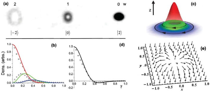
Figure 38: (Color online) Creation of 2D Skyrmions in a spinor BEC. The absorption image (a) of a 2D skyrmion created in spin-2 ⁸⁷Rb. The winding number $\nu_{\text{w}}$ for each spin state is indicated. (b) Azimuthally averaged lineouts (points) for each spin state. (c) 3D plot of the solid lines in (b), where the colors red, green, and blue correspond to the $\left|2\right\rangle$, $\left|0\right\rangle$, and $\left|-2\right\rangle$ states, respectively, with the number of arrowheads indicating the winding number of the spin state. (d) The polarization of the skyrmion. (e) The vector field of the Skyrmion. Reprinted with permission from Leslie et al.[401]. Copyright© (2009) by the American Physical Society.

In 3D, Skyrmion is a particlelike soliton hypothetically introduced by Skyrme [405]. A 3D Skyrmion has a nonsingular texture that can be topologically characterized by a 3D winding number. The stability of a 3D Skyrmion in two-component BECs, which can be simply viewed as a vortex ring containing a superflow, has been theoretically studied and found as metastable solutions of the energy functional [406, 407]. Several schemes have been proposed to create and stabilize the metastable 3D Skyrmions in multi-component BECs [408, 409, 410, 411, 412]. Recently, it was shown that a fully stable 3D Skyrmion can spontaneously emerge as the ground state of a two-component BECs coupled with a synthetic non-Abelian gauge field [413]. The 3D Skyrmion spin texture is elusive in experiments until recently, and it was realized within a spin-polarized ferromagnetic ⁸⁷Rb BEC that is exposed to an externally controlled magnetic field [414].

On the other hand, knots are another 3D topological objects, which are characterized by a linking number or a Hopf invariant [415]. The existence of a stable knot soliton was first discussed in the context of a two-component BEC [416]. An experimental scheme for generation of knot spin textures in a spin-1 BEC was proposed [417]. Based on this theoretical proposal, the creation and observation of knot solitons in the spinor BEC has recently been demonstrated [418].

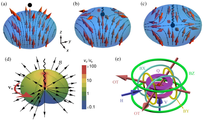
Figure 39: (Color online) Creation of Dirac monopoles in a spinor BEC. (a-c) Spin orientation (red arrows) in the condensate when the magnetic field zero (black dot) is above (a), entering (b) and in the middle of (c) the condensate. The helix represents the singularity in the vorticity. (d) Azimuthal superfluid velocity $v_{s}$ (red arrow and colour scale by equatorial velocity $v_{e}$). Black arrows depict the synthetic magnetic field $B^{*}$. (e) Experimental setup with a controlled 3D magnetic quadrupole. Reprinted by permission from Macmillan Publishers Ltd: Ray et al.[419], copyright© (2014).

A fundamentally important and interesting topological defect is monopole, following Dirac’s theory of magnetic monopoles which are consistent with both quantum mechanics and the gauge invariance of the electromagnetic field [1]. The experimental evidence of magnetic monopoles as fundamental constituents of matter is still absent, however, they can emerge as quasiparticle excitations or other analogies in condensed matter systems, such as topological insulators [420]. It has been proposed that the light-induced gauge potentials for neural atoms in proper Raman laser fields can provide the realization of synthetic magnetic monopoles and even non-Abelian monopoles [421, 92, 422, 423]. Alternatively, it was theoretically demonstrated that a topological defect as the Dirac magnetic monopole can be imprint on the spin texture of an atomic BEC by using external magnetic fields [424]. Due to the spin of the condensate aligning with the local magnetic field with nontrivial 3D structures, one can create a pointlike defect to the spin texture of the condensate giving rise to a vorticity equivalent to the magnetic field of a magnetic monopole. A synthetic monopole field on a sphere with exact flat Landau levels on curved spherical geometry in a system of spinful cold atoms could be realized by engineering of a magnetic quadrupole field [425].

Following the method introduced in Ref. [424], the Dirac monopoles have been experimentally created in the synthetic electromagnetic field that arises in the order parameter of a ferromagnetic spin-1 ⁸⁷Rb BEC in a tailored excited state [419]. The order parameter $\mathit{\Psi}({r},t)=\psi({r},t)\zeta({r},t)$ is the product of a scalar order parameter $\psi$, and a spinor $\zeta=(\zeta_{+1},\zeta_{0},\zeta_{-1})^{\mathrm{T}}\equiv|\zeta\rangle$, where $\zeta_{m}=\langle m|\zeta\rangle$ represents the $m$th spinor component along $z$, with $\zeta=(1,0,0)^{\mathrm{T}}$ at the beginning. The spin texture $\mathbf{S}=\mathit{\Psi}^{\dagger}\mathbf{F}\mathit{\Psi}$ are given by the condensate order parameter and the spin-$1$ matrices $\mathbf{F}$. The spinor order parameter corresponding to the Dirac monopole was generated by an adiabatic spin rotation in response to a time-varying magnetic field [419]

$$\mathbf{B}(r,t)=b_{q}(x\hat{x}+y\hat{y}-2z\hat{z})+B_{z}(t)\hat{z},$$ (212)

where $b_{q}>0$ is the strength of a quadrupole field gradient and $B_{z}(t)$ is a uniform bias field. As shown in Fig. 39, the magnetic field zero is initially located on the $z$ axis at $z=B_{z}(0)/2b_{q}$, and the spin rotation occurs as $B_{z}$ is reduced, drawing the magnetic field zero into the region occupied by the superfluid. In the experiment, the condensate spin nearly adiabatically follows the local direction of the field, as shown in Fig. 39(a-c). Using a scaled and shifted coordinate system with $x^{\prime}=x$, $y^{\prime}=y$, $z^{\prime}=2z-B_{z}/b_{q}$, corresponding spherical coordinates $(r^{\prime},\theta^{\prime},\phi^{\prime})$, the applied magnetic field is then $\mathbf{B}=b_{q}(x^{\prime}\hat{x}^{\prime}+y^{\prime}\hat{y}^{\prime}-z^{\prime}\hat{z}^{\prime})$. As $B_{z}$ is reduced, each spin rotates by an angle $\pi-\theta^{\prime}$ about an axis defined by the unit vector $\hat{n}(r^{\prime},\theta^{\prime},\phi^{\prime})=-\hat{x}^{\prime}\text{sin}\phi^{\prime}+\hat{y}^{\prime}\text{cos}\phi^{\prime}$. In the adiabatic limit, the condensate order parameter corresponds to the local eigenstate of the linear Zeeman operator $g_{F}\mu_{B}\mathbf{B}\cdot\mathbf{F}$, and this spatially-dependent rotation leads to a superfluid velocity [424, 419]

$$\mathbf{v}_{s}=\frac{\hbar}{Mr^{\prime}}\frac{1+\text{cos}\theta^{\prime}}{\text{sin}\theta^{\prime}}{{\hat{\varphi^{\prime}}}},$$ (213)

and vorticity

$$\mathbf{\Omega}_{s}=\nabla^{\prime}\times\mathbf{v}_{s}=-\frac{\hbar}{Mr^{\prime 2}}\hat{r^{\prime}}+\frac{4\pi\hbar}{M}\delta(x^{\prime})\delta(y^{\prime})\mathit{\Theta}(z^{\prime})\hat{r^{\prime}},$$ (214)

where $M$ is the atomic mass, $\delta$ is the Dirac delta function and $\mathit{\Theta}$ is the Heaviside step function. The vorticity is a monopole attached to a semi-infinite vortex line singularity as an analog of Dirac string, with phase winding $4\pi$, extending along the positive $z^{\prime}$ axis. The synthetic vector potential arising from the spin rotation can be written as $\mathbf{A}^{*}=-M{\mathbf{v}_{s}}/\hbar$, and the synthetic magnetic field of the monopole is

$$\mathbf{B}^{*}=\frac{\hbar}{r^{\prime 2}}\hat{r}^{\prime}.$$ (215)

The fields $\mathbf{v}_{s}$ and $\mathbf{B}^{*}$ are depicted in Fig. 39(d). The created Dirac monopoles were then experimentally identified at the termini of vortex lines within the condensate by directly imaging such a vortex line in real space [419]. Based on this method, a topological point defect as an isolated monopole without terminating nodal lines (the Dirac string) was also created and observed in the order parameter of the spin-1 BEC [426].

6.3 Spin Hall effect in atomic gases

Spin Hall effects [427] are a class of SOC phenomena where flowing particles experience orthogonally directed spin-dependent Lorentz-like forces and give rise spin currents. This is analogous to the conventional Lorentz force for the Hall effect, but opposite in sign for two spin states. A quantized spin Hall effect is closely related to the $\mathbb{Z}_{2}$ topological insulators which preserves time-reversal symmetry (see Sec. 4.2.4 and 4.3.4). The spin Hall effects have been observed for electrons in spin-orbit coupled materials [428, 429] and circularly polarized photons passing through certain surfaces [430, 431]. It was proposed that the spin Hall effects can be realized for neutral atoms with spin-dependent Lorentz forces [84, 108], which can be achieved by the synthetic gauge potentials as discussed in Sec. 3.4. Following the proposal of Ref. [84], the spin Hall effect was observed in a pseudospin-1/2 ⁸⁷Rb BEC subjected to spin- and space-dependent vector potentials [104].

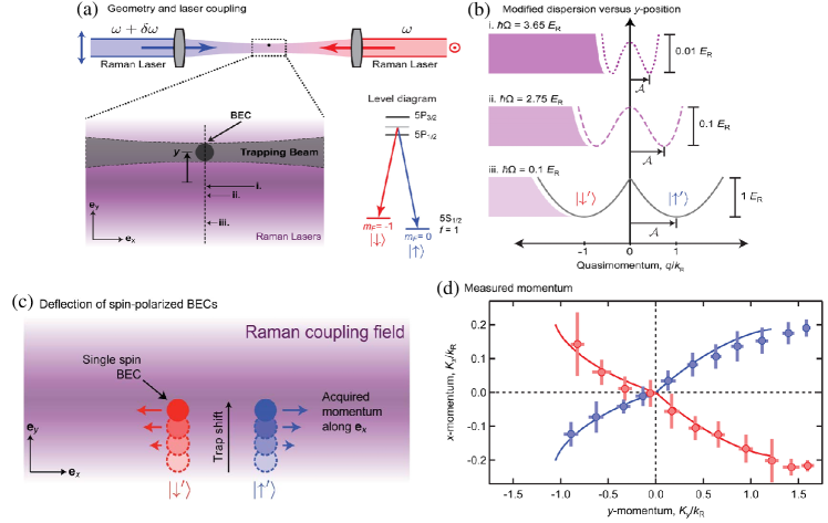
Figure 40: (Color online) Atomic spin Hall effect. (a) Experiment schematic of two controlled Raman beams propagating along $\hat{x}$ coupled two ground states in ⁸⁷Rb atoms. (b) The induced double-well dispersion $E(q)$ for the three different $y$-positions marked in (a), with the synthetic vector potentials $\mathcal{A}$. (c) Spin Hall effect with spin-dependent forces along $\hat{x}$ from motion along $\hat{y}$. (d) Acquired momentum along $\hat{x}$ versus final momentum along $\hat{x}$. Reprinted by permission from Macmillan Publishers Ltd: Beeler et al.[104], copyright© (2013).

Experimentally, two Raman lasers counterpropagating with wave number $k_{R}$ along $\hat{x}$ were used to couple the internal states $\left|f=1;m_{F}=0,-1\right>=|\uparrow,\downarrow\rangle$, which comprise pseudospin-$1/2$ atomic system with strength $\Omega$, as shown in Fig. 40(a). For $\hbar\Omega<4E_{\rm{R}}$ with the single-photon recoil energy $E_{\rm{R}}$, the 2D effective pseudospin Hamiltonian (ignoring the trap, the light shift and the zero-energy shift from the Raman dressing) can be written as [104]

$$\hat{H}=\frac{1}{2m}\left(\mathbf{\hat{p}}-\mathcal{A}\hat{\sigma}_{z}\mathbf{e}_{x}\right)^{2},$$ (216)

where $\mathcal{A}=\hbar k_{\rm{R}}\left[1-\left(\hbar\Omega/4E_{\rm{R}}\right)^{2}\right]^{1/2}$ is a light-induced spin-dependent vector potential along $\hat{x}$. As shown in Fig. 40(b), the modified dispersion features two degenerate wells and each of them displaces from zero by an amount $\mathcal{A}$. Here $\mathcal{A}$ has the spatial dependence of the Raman lasers’ Gaussian intensity profile since $\Omega$ depends on the laser intensity. The spatial dependence of $\mathcal{A}$ gives rise to a spin Hall effect in the atomic gas [84, 108]. In the experiment [104], the mechanism underlying the spin Hall effect was first probed from observing spin-dependent shear in the atomic density distribution by abruptly changing $\mathcal{A}$, which gives rise to a spin-dependent “electric” force $-\partial\mathcal{A}/\partial t$ on the atom cloud. Then for a time-independent $\mathcal{A}$, the resulting spin Hall effect was further observed by detecting a spin-dependent Lorentz-like response along $\pm\hat{x}$ with atoms propelled in either spin state along $\hat{y}$ and realizing an atomic spin transistor using a mixture of both spins. As shown in Fig 40(c,d), each spin-polarized BEC acquired a momentum along $\hat{x}$ that was detected oppositely for the two spins and related to its final momentum along $\hat{y}$, which demonstrates an intrinsic spin Hall effect.

Since the (pseudo)spin here is a good quantum number, the system can be thought of as two independent subsystems that respond oppositely to temporal and spatial gradients of the light-induced gauge potential $\mathcal{A}$. By introducing a large non-zero curl for $\mathcal{A}$, each spin state could be separately driven to the regime of integer QHE [84, 104]. Therefore, one can create a quantum spin Hall effect in this atomic system composed of an equal mixture of both spins.

7 Topological matter with interactions

Until now we have mainly reviewed cold-atom realizations of essentially non-interacting topological phases. But interactions can lead to new topological phases including intrinsic topological phases and symmetry-protected topological phases for both bosonic and fermionic systems in all dimensions. While tremendous theoretical efforts have been recently paid with fruitful achievements usually by advanced mathematics, the experimental realization for most theoretically predicted phases hardly has any solid progress yet except several classic examples. This section is intended not to give a systematical review of interacting topological phases, which is beyond the scope of this review article, but much more modestly to introduce a number of interesting models with interactions, which can exhibit interaction-intrinsic topological phases. In particular we focus on how to realize them by recent advances of cold-atom techniques, and wish to convey the expectation that the high-tunability of cold-atom systems would enable us to explore this open and deep field further.

7.1 Spin chains

7.1.1 Spin-1/2 chain

Ultracold atoms in OLs is a promising platform to realize some spin-1/2 models. We here consider the well-know anisotropic Heisenberg model (XXZ model) in 1D, which arises in the context of various condensed matter systems. The Hamiltonian of XXZ spin model is given by

$$H_{\text{XXZ}}=-\sum_{j=1}^{N}\left[\lambda_{z}\sigma_{j}^{z}\sigma_{j+1}^{z}+\lambda_{\perp}\left(\sigma_{j}^{x}\sigma_{j+1}^{x}+\sigma_{j}^{y}\sigma_{j+1}^{y}\right)\right],$$ (217)

where $\lambda_{z}$ ($\lambda_{\perp})$ denotes the nearest neighbor interaction along $z$-direction ($x-$ and $y$-direction), and $\sigma^{x,y,z}_{j}$ are the Pauli matrices for the $j$th spin. The phase diagram of this Hamiltonian is pretty rich. In addition, the geometric phase of the ground state in this spin model is quantized in certain parameters and it obeys scaling behavior in the vicinity of a quantum phase transition[432, 433].

When $\lambda_{\perp}=0$ and in the presence of an applied magnetic field along $x$ direction, the model in Eq.(217) becomes the transverse Ising model, which Hamiltonian is given by

$$H_{\text{Ising}}=-\lambda_{z}\sum_{j=1}^{N-1}\sigma_{j}^{z}\sigma_{j+1}^{z}-h_{x}\sum_{j=1}^{N}\sigma_{j}^{x},$$ (218)

where the parameter $h_{x}$ is the intensity of the magnetic field applied in the $x$ direction. Consider the projection onto the $x$-axis of the spin with the fermionic occupation number $n$: $|\uparrow\rangle\leftrightarrow n=0,\leavevmode\nobreak\ \leavevmode\nobreak\ |\downarrow\rangle\leftrightarrow n=1$, one has $\sigma_{j}^{x}=(-1)^{a_{j}^{\dagger}a_{j}}$. Employing the string-like annihilation and creation operators (the Jordan-Wigner transformation):

$$a_{j}=\left(\prod_{k=1}^{j-1}\sigma_{k}^{x}\right)\sigma_{j}^{+},\leavevmode\nobreak\ \leavevmode\nobreak\ a_{j}^{\dagger}=\left(\prod_{k=1}^{j-1}\sigma_{k}^{x}\right)\sigma_{j}^{-},$$ (219)

where $\sigma^{+}$ and $\sigma^{-}$ are the spin raising and lower operators, $H_{\text{Ising}}$ can be rewritten as

$$H_{\text{Ising}}=J\sum_{j=1}^{N-1}(a_{j}-a_{j}^{\dagger})(a_{j+1}+a_{j+1}^{\dagger})+2h_{z}\sum_{j=1}^{N}\left(a_{j}^{\dagger}a_{j}-1/2\right).$$ (220)

This shows that the 1D transverse Ising chain is mathematically equivalent to the Kiteav’s chain [434] of p-wave superconductor (see the next section) and thus exhibits the same topological phase, in which the ground state degeneracy is dependent on the boundary conditions of the chain. For the superconductors, the $\mathbb{Z}_{2}$ symmetry of fermionic parity cannot be lifted by any local physical operators, because such operators must contain an even number of fermion operators. However, the $\mathbb{Z}_{2}$ symmetry in the Ising model is given by a global spin flip in the $\sigma_{z}$ basis: $P_{S}=\prod_{j=1}^{N}\sigma_{j}^{x}$, such that its degeneracy can be lifted by a simple longitudinal magnetic field $h_{z}\sum_{j}\sigma_{j}^{z}$. This indicates that the topological phase in the transverse Ising chain is much weaker, and thus the creation and manipulation of Majorana edge modes in this system are more difficult.

We now turn to address a scheme proposed in Ref. [435] to realize the spin models with ultracold atoms in OLs. Consider an ensemble of ultracold bosonic or fermionic atoms confined in an OL. We are interested in the Mott insulator regime, and the atomic density of roughly one atom per lattice site. Each atom is assumed to have two relevant internal states, which are denoted with the effective spin index $\sigma=\uparrow,\downarrow$, respectively. We assume that the atoms with spins $\sigma=\uparrow,\downarrow$ are trapped by independent standing wave laser beams through polarization (or frequency) selection. Each laser beam creates a periodic potential $V_{\mu\sigma}\text{sin}^{2}(\vec{k}_{\mu}\cdot\vec{r})$ in a certain direction $\mu$, where $\vec{k}_{\mu}$ is the wavevector of light. For sufficiently strong periodic potential and low temperatures, the atoms will be confined to the lowest Bloch band, and the low energy Hamiltonian is then given by the Boson- or Fermi-Hubbard Hamiltonian

$$H=-\sum_{\langle ij\rangle\sigma}\left(J_{\mu\sigma}a_{i\sigma}^{\dagger}a_{j\sigma}+H.c.\right)+\frac{1}{2}\sum_{i,\sigma}U_{\sigma}n_{i\sigma}\left(n_{i\sigma}-1\right)+U_{\uparrow\downarrow}\sum_{i}n_{i\uparrow}n_{i\downarrow},$$ (221)

where $\left\langle i,j\right\rangle$ denotes the near neighbor sites, $a_{i\sigma}$ are bosonic (or fermionic) annihilation operators respectively for bosonic (or fermionic) atoms of spin $\sigma$ localized on site $i$, and $n_{i\sigma}=a_{i_{\sigma}}^{\dagger}a_{i_{\sigma}}$.

For the cubic lattice ($\mu=x$,$y$,$z$) and using a harmonic approximation around the minima of the potential, the spin-dependent tunneling energies and the on-site interaction energies are given by

$$J_{\mu\sigma}\approx\frac{4E_{R}^{1/4}\left(V_{\mu\sigma}\right)^{3/4}}{\sqrt{\pi}}e^{-2(V_{\mu\sigma}/E_{R})^{1/2}},\ U_{\uparrow\downarrow}\approx\left(\frac{8}{\pi}\right)^{1/2}(ka_{s\uparrow\downarrow})(E_{R}\overline{V}_{1\uparrow\downarrow}\overline{V}_{2\uparrow\downarrow}\overline{V}_{3\uparrow\downarrow})^{1/4},$$

$$U_{\sigma}\approx\left(\frac{8}{\pi}\right)^{1/2}\left(ka_{s\sigma}\right)\left(E_{R}V_{1\sigma}V_{2\sigma}V_{3\sigma}\right)^{1/4}\ (\text{for bosons}),U_{\sigma}\approx 2\sqrt{V_{\mu\sigma}E_{R}}\ (\text{for fermions}),$$

where $\overline{V}_{\mu\uparrow\downarrow}=4V_{\mu\uparrow}V_{\mu\downarrow}/(V_{\mu\uparrow}^{1/2}+V_{\mu\downarrow}^{1/2})^{2}$ is the spin average potential in each direction, $E_{R}=\hbar^{2}k^{2}/2m$ is the atomic recoil energy, and $a_{s\uparrow\downarrow}$ is the scattering length between the atoms of different spins. For fermionic atoms, $U_{\sigma}$ is on the order of Bloch band separation $\sim 2\sqrt{V_{\mu\sigma}E_{R}}$, which is typically much larger than $U_{\uparrow\downarrow}$ and can be taken to be infinite. In writing Eq.(221), overall energy shifts $\sum_{i\mu}\left(\sqrt{E_{R}V_{\mu\uparrow}}-\sqrt{E_{R}V_{\mu\downarrow}}\right)\left(n_{i\uparrow}-n_{i\downarrow}\right)/2$ have been neglected, which can be easily compensated by a homogeneous external magnetic field applied in the $z$ direction.

From the above expressions, we observe that $J_{\mu\sigma}$ depend sensitively (exponentially) upon the ratios $V_{\mu\sigma}/E_{R}$ while $U_{\uparrow\downarrow}$ and $U_{\sigma}$ exhibit only weak dependence. So we can easily introduce spin-dependent tunneling $J_{\mu\sigma}$ by varying the potential depth $V_{\mu\uparrow}$ and $V_{\mu\downarrow}$ with control of the intensity of the trapping laser. This simple experimental method provides us a powerful tool to engineer many-body Hamiltonians. In the regime where $J_{\mu\sigma}\ll U_{\sigma},U_{\uparrow\downarrow}$ and $\left\langle n_{i\uparrow}\right\rangle+\left\langle n_{i\downarrow}\right\rangle\simeq 1$, which corresponds to an insulating phase, the terms proportional to tunneling $J_{\mu\sigma}$ can be considered via perturbation theory. To the leading order in $J_{\mu\sigma}/U_{\uparrow\downarrow}$, Eq. (221) is equivalent to the following effective Hamiltonian

$$H=-\sum_{j=1}^{N}\left[\lambda_{\mu z}\sigma_{j}^{z}\sigma_{j+1}^{z}+\lambda_{\mu\perp}\left(\sigma_{j}^{x}\sigma_{j+1}^{x}+\sigma_{j}^{y}\sigma_{j+1}^{y}\right)\right],$$ (222)

where $\sigma_{i}^{z}=n_{i\uparrow}-n_{i\downarrow}$, $\sigma_{i}^{x}=a_{i\uparrow}^{\dagger}a_{i\downarrow}+a_{i\downarrow}^{\dagger}a_{i\uparrow}$, and $\sigma_{i}^{y}=-i\left(a_{i\uparrow}^{\dagger}a_{i\downarrow}-a_{i\downarrow}^{\dagger}a_{i\uparrow}\right)$ are the usual spin operators. The $+$ and $-$ signs before $\lambda_{\mu\perp}$ correspond, respectively, to the cases of fermionic and bosonic atoms. The parameters $\lambda_{\mu z}$ and $\lambda_{\mu\perp}$ for the bosonic atoms are given by

$$\lambda_{\mu z}=\frac{J_{\mu\uparrow}^{2}+J_{\mu\downarrow}^{2}}{2U_{\uparrow\downarrow}}-\frac{J_{\mu\uparrow}^{2}}{U_{\uparrow}}-\frac{J_{\mu\downarrow}^{2}}{U_{\downarrow}},\;\;\lambda_{\mu\perp}=\frac{J_{\mu\uparrow}J_{\mu\downarrow}}{U_{\uparrow\downarrow}}.$$ (223)

For fermionic atoms the expression for $\lambda_{\perp}$ is the same as in (223), but in the expression for $\lambda_{z}$ the last two terms vanish since $U_{\sigma}\gg U_{\uparrow\downarrow}$. In writing Eq. (222), the term $\sum_{i\mu}4\left(J_{\mu\uparrow}^{2}/U_{\uparrow}-J_{\mu\downarrow}^{2}/U_{\downarrow}\right)\sigma_{i}^{z}$ is neglected, since it can be easily compensated by an applied external magnetic field. When we set $V_{\mu\downarrow}/V_{\mu\uparrow}\gg 1$, so that $J_{\mu\downarrow}$ becomes negligible while $J_{\mu\uparrow}$ remains finite. In this case, the Hamiltonian (222) reduces to the Ising model $H=\sum_{\left\langle i,j\right\rangle}\lambda_{\mu z}\sigma_{i}^{z}\sigma_{j}^{z}$, with $\lambda_{\mu z}=J_{\mu\uparrow}^{2}/\left(1/2U_{\uparrow\downarrow}-1/U_{\uparrow}\right)$. The transverse field term in Eq.(218) can be easily achieved with an applied external magnetic field along the $x$ direction. The Ising model has been realized experimentally with atoms in OLs [436, 437].

The approach using ultracold atoms to realize the spin models has a unique advantage in that the parameters $\lambda_{\mu z}$ and $\lambda_{\mu\perp}$ can be easily controlled by adjusting the intensity of the trapping laser beams. They can also be changed within a broad range by tuning the ratio between the scattering lengths $a_{s\uparrow\downarrow}$ and $a_{s\sigma}$ $\left(\sigma=\uparrow,\downarrow\right)$ by adjusting an external magnetic field through Feshbach resonance. Therefore, even with bosonic atoms alone, it is possible to realize the entire class of Hamiltonians in the general form (222) with an arbitrary ratio $\lambda_{\mu z}/\lambda_{\mu\perp}$. This is important since bosonic atoms are generally easier to cool. We estimate the typical energy scales for the realized Hamiltonian. For Rb atoms with a lattice constant $\pi/\left|\vec{k}\right|\sim 426$nm, the typical tunnelling rate $J/\hbar$ can be chosen from zero to a few kHz. The on-site interaction $U/\hbar$ corresponds to a few kHz at zero magnetic field, but can be much larger near the Feshbach resonance. The energy scale for magnetic interaction is about $J^{2}/\hbar U\sim 0.1$kHz (corresponding to a time scale of $10$ms) with a conservative choice of $U\sim 2$kHz and $\left(J/U\right)^{2}\sim 1/20$.

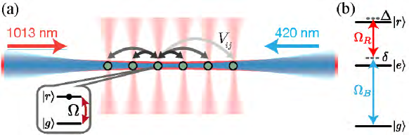
Figure 41: (Color online) Experimental platform for realization of the Ising model. (a) Individual ⁸⁷Rb atoms are trapped using optical tweezers (vertical red beams) and arranged into defect-free arrays. Coherent interactions $V_{ij}$ between the atoms are enabled by exciting them to a Rydberg state with strength $\Omega$ and detuning $\Delta$. (b) A two-photon process couples the ground state $|g\rangle=|5S_{1/2},F=2,m_{F}=-2\rangle$ to the Rydberg state $|r\rangle=|70S_{1/2},J=1/2,m_{J}=-1/2\rangle$ via an intermediate state $|e\rangle=|6P_{3/2},F=3,m_{F}=-3\rangle$ with detuning $\delta$, using circularly polarized 420 nm and 1013 nm lasers with single-photon Rabi frequencies of $\Omega_{B}$ and $\Omega_{R}$, respectively. Reprinted by permission from Macmillan Publishers Ltd: Bernien et al. [438], copyright© (2017).

Furthermore, the Ising model with long range interactions can be realized with the Rydberg gas in OLs [439, 440, 441, 438]. A promising avenue for realizing strongly interacting quantum matter involves coherent coupling of neutral atoms to highly excited Rydberg states. This results in repulsive van der Waals interactions of strength $V_{ij}=C/R_{ij}^{6}$ between Rydberg atom pairs at a distance $R_{ij}$, where $C$ is the van der Waals coefficient. Such interactions have recently been used to explore quantum many-body physics of Ising spin systems in OLs [439, 440, 441, 438]. The achieved Hamiltonian $(\hbar=1)$ is given by

$$\tilde{H}_{\text{Ising}}=\sum_{i}\frac{\Omega_{i}}{2}\sigma_{i}^{x}-\sum_{i}\Delta_{i}n_{i}+\sum_{i<j}V_{ij}n_{i}n_{j},$$ (224)

where $\Delta_{i}$ are the detunings of the driving lasers from the Rydberg state, $\Omega_{i}$ is the Rabi frequency describing the coupling between the ground state $|g_{i}\rangle$ and the Rydberg state $|r_{i}\rangle$ of an atom at position $i$, and $n_{i}\rangle=|r_{i}\rangle\langle r_{i}|$. The Hamilton with the first two terms in Eq. (224) is equivalent to the Ising Hamiltonian in Eq. (218), while the last term represents the long range interactions induced by the van der Waals interactions. Recently a programmable Ising-type quantum spin model with tunable interactions and system sizes of up to 51 qubits was experimentally realized [438]. Their approach combines these strong, controllable interactions with atom-by-atom assembly of arrays of cold neutral ⁸⁷Rb atoms. The experimental platform is shown in Fig. 41, each ⁸⁷Rb atoms can be controlled by optical tweezers, the parameters ($|\Omega_{i}|=\Omega$ and $\Delta_{i}=\Delta$) can be controlled by changing laser intensities and detunings in time. The interaction strength $V_{ij}$ can be tuned either by varying the distance between the atoms or by coupling them to a different Rydberg state.

7.1.2 Spin-1 chain and Haldane phase

Another topological spin model is the spin-1 quantum Heisenberg chain, with the ground state belonging to the Haldane phase [9, 442]. In the topological aspect, the Haldane phase is protected by the lattice inversion symmetry and can be classified as a symmetry-protected topological phase [443, 444]. According to Haldane’s seminal work [9, 442], the 1D integer-spin Heisenberg antiferromagnets have an exotic unordered ground state with unbroken rotational symmetry and with a finite excitation gap in the spectrum, while half-integer antiferromagnets are gapless. There are two topological features of the Haldane insulator phase: the existence of hidden non-local string order [445] and emergent fractional spin-1/2 edge states at the boundaries of open chains [446]. For integer spin $S=1$, the following quadratic-biquadratic Hamiltonian contains the Haldane phase in a rich phase structure [447, 448, 449]:

$$H_{\rm QB}=\alpha\sum_{j=1}^{N-1}\left[\mathbf{S}_{j}\cdot\mathbf{S}_{j+1}+\beta(\mathbf{S}_{j}\cdot\mathbf{S}_{j+1})^{2}\right],$$ (225)

where $\beta$ is a relative coupling constant, the sign of $\alpha$ determines the ferro or antiferromagnetic regimes, and $\mathbf{S}_{j}=(S_{j}^{x},S_{j}^{y},S_{j}^{z})$ are spins at lattice site $j$ with

$$S_{j}^{x}=\frac{1}{\sqrt{2}}\left(\begin{array}[]{ccc}0&1&0\\ 1&0&1\\ 0&1&0\\ \end{array}\right),\ \ S_{j}^{y}=\frac{1}{\sqrt{2}}\left(\begin{array}[]{ccc}0&-i&0\\ i&0&-i\\ 0&i&0\\ \end{array}\right),\ \ S_{j}^{z}=\left(\begin{array}[]{ccc}1&0&0\\ 0&0&0\\ 0&0&-1\\ \end{array}\right).$$ (226)

The properties of the ground state of $H_{\rm QB}$ are entirely determined by an angle, $\theta$, such that $\alpha=|a|\text{cos}\theta$ and $\alpha\beta=|a|\text{sin}\theta$. The ground state belongs to the Haldane phase when $\theta\in[-\frac{\pi}{4},\frac{\pi}{4}]$, with $\theta=0$ being the Heisenberg point and $\theta=\arctan(\frac{1}{3})$ the Affleck-Lieb-Kennedy-Tasaki point [447, 448], which can be described with an exact valence-bond wavefunction. There are two critical points $\theta=\pm\frac{\pi}{4}$, at which a phase transition occurs into a gapless phase for $\theta\in[\frac{\pi}{4},\frac{\pi}{2}]$ and into a gapped dimerized phase for $\theta\in[-\frac{3\pi}{4},-\frac{\pi}{4}]$, respectively. For other values of $\theta$, the ground state belongs to the ferromagnetic phase.

Although the Haldane phase of integer-spin Heisenberg antiferromagnets has been extensively studied in theories in the last decades, to the best of our knowledge, there is no experimentally convenient system for realzing this phase. Recently, it has been proposed that the Haldane phase can be explored with ultracold atoms in OLs thanks to the high tunability in these systems. A first possible direction is to use spin-1 bosonic atoms in a deep 1D OL with one atom per site [449], which can be described by the following extended Bose-Hubbard Hamiltonian:

$$H_{BH}=-J\sum_{\langle{j,l}\rangle,\alpha}(a^{\dagger}_{j\alpha}a_{l\alpha}+a^{\dagger}_{l\alpha}a_{j\alpha})+\sum_{S=0,2}\frac{U_{S}}{2}\sum_{j,\alpha,\beta,\gamma,\delta}(\Psi^{(S)}_{\gamma\delta}a_{j\gamma}a_{j\delta})^{\dagger}(\Psi^{(S)}_{\alpha\beta}a_{j\alpha}a_{j\beta}).$$ (227)

Here the indices $j$ and $l$ run over the lattice sites, the Greek letters label the three spin-component of an atom ($\alpha,\beta,\gamma,\delta=-1,0,+1$). Then the first term in the Hamiltonian is the single-particle hopping with amplitude $J$, and the second term describes the interaction between bosons within a site. Two bosons interact only when their total spin is either $0$ or $2$ because the state $S=1$ is antisymmetric, and the interaction may be different for each value of the total spin. This is taken into account by the spin-dependent interaction constants $U_{S}$ and the tensors $\Psi^{(S)}_{\gamma\beta}=\langle{S|s,\gamma;s,\beta}\rangle$, which are the Clebsch-Gordan coefficients between the states $|s=1,\gamma\rangle\otimes|s=1,\beta\rangle$ and $|S=0,2\rangle$. For the case of one atom per site, one can define the effective spin-1 operators

$$S_{j}^{z}=a^{\dagger}_{j,+1}a_{j,+1}-a^{\dagger}_{j,-1}a_{j,-1},\ \ S_{j}^{+}=(S_{j}^{-})^{{\dagger}}=a^{\dagger}_{j,+1}a_{j,0}+a^{\dagger}_{j,0}a_{j,-1},$$

where $S_{j}^{\pm}=S_{j}^{x}\pm S_{j}^{y}$. Using a perturbative calculation for $J\ll U_{S}$ and around states with unit occupation, one can obtain the Hamiltonian $H_{QB}$ in Eq. (225) from the Hamiltonian $H_{BH}$ in Eq.(227) with the parameters $\alpha=\tfrac{1}{2}C_{2}$, $\beta=\tfrac{1}{3}(2C_{0}/C_{2}+1)$, where $C_{S}=J^{2}/U_{S}$ is tunable in the OL. The ways for adiabatically preparing the Haldane phase and detecting its intrinsic properties (the energy gap, end-chain spins effects and the string order parameter) in the OL have also been proposed [449].

Sequent studies to realize the Haldane phase have been made on spinless bosons with long-range dipole interactions in 1D OLs [450, 451, 452, 453, 454, 455], where the effective spin-1 chain can be obtained by truncating the Hilbert space of the Bose system to three occupation states per site. The Haldane insulators were also predicted for two-component [456, 457, 458, 459] and multi-component [460, 461, 462] Fermi gases in 1D OLs. A two-leg spin-1/2 ladder, which can be realized with cold atoms in a ladder-like OL, was also shown to host a Haldane-like phase [463, 464, 465]. A gapless topological Haldane liquid phase in a 1D cold polar molecular lattice and an exotic topological Haldane superfluid phase of soft-core bosons in 1D OLs were predicted [466, 467]. Recently, the direct observation of hidden non-local string order via quantum gas microscopy of doped ultracold Fermi-Hubbard chains was reported [468], which is an important step toward experimental studies of emergent topological order in integer spin chains.

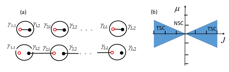
Figure 42: (Color online) Two phases of the Kitaev chain. (a) Upper: In the topological trivial phase Majorana fermions on each lattice site can be thought of as bound into ordinary fermions. Lower: In the topological nontrivial phase Majorana fermions on neighboring sites are bound leaving two unpaired Majorana fermions at the two ends of the chain. (b) The phase diagram of the Kitaev chain in the $\mu-J$ plane, showing the topological superconducting phase and the normal superconducting phase.

7.2 Kitaev chain model

The well-known Kitaev chain was proposed by Alexei Kitaev [469], which is the simplest model system that shows unpaired Majorana zero modes. The Kitaev model is a toy model but can be exactly solved, which provides an extremely useful paradigm for Majorana zero modes at the two ends of a quantum wire of $p$-wave superconductor. The Kitaev chain is the spinless fermion model with nearest-neighbor hopping and pairing between the sites of a 1D lattice described by the Hamiltonian

$$H=\sum_{j}[-J(c^{\dagger}_{j}c_{j+1}+c^{\dagger}_{j+1}c_{j})-\mu(c^{\dagger}_{j}c_{j}-\frac{1}{2})+\Delta{c_{j}c_{j+1}}+\Delta^{*}c^{\dagger}_{j+1}c^{\dagger}_{j}],$$ (228)

where $\mu$ is a chemical potential, and $\Delta=|\Delta|e^{i\theta}$ is a superconducting gap. Consider a chain with $L$ sites and open boundary conditions, as shown in Fig.(42), we can rewrite this Hamiltonian in the Majorana representation by using the Majorana operators as

$$H=\frac{i}{2}\sum_{j}[-\mu\gamma_{j,1}\gamma_{j,2}+(J+|\Delta|)\gamma_{j,2}\gamma_{j+1,1}+(-J+|\Delta|)\gamma_{j,1}\gamma_{j+1,2}].$$ (229)

Here the Majorana operators are defined as

$$\gamma_{j,1}=e^{i\frac{\theta}{2}}c_{j}+e^{-i\frac{\theta}{2}}c_{j}^{\dagger},\leavevmode\nobreak\ \leavevmode\nobreak\ \leavevmode\nobreak\ \leavevmode\nobreak\ \gamma_{j,2}=(e^{i\frac{\theta}{2}}c_{j}-e^{-i\frac{\theta}{2}}c_{j}^{\dagger})/i.$$ (230)

which satisfy the relations

$$\gamma^{\dagger}_{j,\alpha}=\gamma_{j,\alpha},\leavevmode\nobreak\ \leavevmode\nobreak\ \leavevmode\nobreak\ \{\gamma_{j,\alpha},\gamma_{k,\beta}\}=2\delta_{jk}\delta_{\alpha\beta},$$ (231)

for $j,k=1,2,...,L$ and $\alpha,\beta=1,2$.

Now we discuss two specific cases. The topological trivial case for $|\Delta|=J=0$ is considered first. The Hamiltonian becomes

$$H=-\mu\sum_{j}(c^{\dagger}_{j}c_{j}-\frac{1}{2})=\frac{i}{2}(-\mu)\sum_{j}\gamma_{j,1}\gamma_{j,2}.$$ (232)

The Majorana operators $\gamma_{j,1}$, $\gamma_{j,2}$ from the same site $j$ are paired together, as shown in Fig. 42(a), to form a ground state with the occupation number $0$ ($\mu<0$) or $1$ ($\mu>0$). Secondly, we consider the cases of $|\Delta|=J>0$ and $\mu=0$, and we have

$$H=iJ\sum^{L-1}_{j}\gamma_{j,2}\gamma_{j+1,1}.$$ (233)

Now the Majorana operators $\gamma_{j,2}$ and $\gamma_{j+1,1}$ from different sites are paired together, as illustrated in Fig. 42(a). The ground state of this Hamiltonian is easily found by defining new annihilation and creation operators

$$a_{j}=\frac{1}{2}(\gamma_{j,2}+i\gamma_{j+1,1}),\leavevmode\nobreak\ \leavevmode\nobreak\ \leavevmode\nobreak\ a^{\dagger}_{j}=\frac{1}{2}(\gamma_{j,2}-i\gamma_{j+1,1}),$$ (234)

with $i\gamma_{j,2}\gamma_{j+1,1}=2a^{\dagger}_{j}a_{j}-1$ for $j=1,2,...,L-1$. Subsequently, the Hamiltonian (233) can be rewritten in a canonical form

$$H=2J\sum^{L-1}_{j}a^{\dagger}_{j}a_{j}-J(L-1).$$ (235)

As we can see that Hamiltonian (233) does not contain operators $\gamma_{1,1}$ and $\gamma_{L,2}$, i.e., $[\gamma_{1,1},H]=[\gamma_{L,2},H]=0$, while all pairs of ($\gamma_{j,2}$, $\gamma_{j+1,1}$) for $j=1,2,...,L-1$ form new fermions. The ground states with twofold degeneracy for $J>0$ satisfy the condition $a_{j}{|g\rangle}=0$ for all $j$, and

$$H|g\rangle=-J(L-1)|g\rangle.$$ (236)

These represent zero-energy Majorana modes localized at the two ends of the chain. Since $[\gamma_{1,1},H]=[\gamma_{L,2},H]=0$, the two orthogonal ground states of the Kitaev chain model can be constructed as $|g\rangle$ and $a^{\dagger}|g\rangle$, where $a=\frac{1}{2}(\gamma_{1,1}+i\gamma_{L,2})$ is an ordinary zero-energy fermion operator. These states have different fermionic parities: one is even and the other is odd (i.e., it is a superposition of states with even or odd number of electrons). Note that the ground states with double degeneracies or not reveal that the system is topologically nontrivial or trivial, respectively. Similarly, the considerations will also yield unpaired Majorana zero modes for the special case $|\Delta|=-J$ and $\mu=0$. These two specific cases represent two distinct phases of the Kitaev chain: topologically trivial or nontrivial, corresponding to different pairing methods without or with unpaired Majorana zero modes localized at the ends of the chain.

To study the general properties of the Hamiltonian (228) at arbitrary values of $J$, $\mu$ and $\Delta$, we diagonalize the Kitaev Hamiltonian under periodic boundary condition. After the Fourier transformation with $c^{\dagger}_{j}=1/\sqrt{L}\sum_{k}c^{\dagger}_{k}e^{i\mathbf{k}\cdot\mathbf{r}_{j}}$, the Hamiltonian in momentum space can be written in Bogoliubov-de Gennes form

$$H=\frac{1}{2}\sum_{k}\begin{pmatrix}c^{\dagger}_{k}&c_{-k}\end{pmatrix}\mathcal{H}_{\text{BdG}}(k)\begin{pmatrix}c_{k}\\ c^{\dagger}_{-k}\end{pmatrix},$$ (237)

where the Bogoliubov-de Gennes Hamiltonian is written in terms of Pauli matrices $\vec{\tau}$ as

$$\mathcal{H}_{\text{BdG}}(k)=\epsilon(k)\tau_{z}+\Delta(k)\text{cos}\theta\tau_{y}+\Delta(k)\text{sin}\theta\tau_{x},$$ (238)

with $\epsilon(k)=-2J\text{cos}k-\mu$, $\Delta(k)=2|\Delta|\text{sin}k$. The energy spectrum is given by

$$E(k)=\pm\sqrt{\epsilon(k)^{2}+|\Delta(k)|^{2}}.$$ (239)

For $\Delta\neq 0$, the system is in superconducting states. The energy spectrum always fully gapped except when $2J=\pm\mu$. As shown in Fig. 42(b), two lines represent gap closing are defined, which mark the phase transition between the two distinct phases of the model. We can identify that the system in the region $|J|>|\mu|/2$ is a topological superconductor. In the other region, the system is a normal superconductor (topologically trivial).

Since the two distinct phases of the model have the same symmetries but different topological features, we can distinguish these two phases by calculating the topological invariants. As is known, $\mathcal{H}_{\text{BdG}}$ preserves intrinsic particle-hole symmetry. One can check that the Hamiltonian (238) satisfies the relation

$$\hat{C}\mathcal{H}_{\text{BdG}}(k)\hat{C}^{-1}=-\mathcal{H}_{\text{BdG}}(-k),$$ (240)

where the particle-hole operator $\hat{C}=\tau_{x}\hat{K}$ satisfies $\hat{C}^{2}=+1$. According to the topological classifications, Hamiltonian (238) belongs to the symmetry class D $(d=1)$ and thus has a $\mathbb{Z}_{2}$-type topological number. The relevant topological invariant of the system described by the Hamiltonian (228) is the so-called Majorana number $\mathcal{M}=\pm 1$, which is actually the $\mathbb{Z}_{2}$ index, first formulated by Kitaev. In Kitaev’s paper [469], it was shown that all 1D fermionic systems with superconducting order fall into two categories distinguished by $\mathcal{M}$. One is topologically trivial with $\mathcal{M}=+1$ and the other is nontrivial with $\mathcal{M}=-1$ and the existence of unpaired Majorana zero modes.

To calculate $\mathcal{M}$, we consider the Hamiltonian that can be written in the Majorana representation as

$$H=\frac{i}{4}\sum_{lm\alpha\beta}B_{\alpha\beta}(l-m)\gamma_{l\alpha}\gamma_{m\beta},$$ (241)

where $l$ and $m$ label the lattice sites while $\alpha$ and $\beta$ denote all other quantum numbers. Then $\mathcal{M}$ is defined as

$$\mathcal{M}=\text{sgn}\{\text{Pf}[\tilde{B}(0)]\}\text{sgn}\{\text{Pf}[\tilde{B}(\pi)]\}$$ (242)

where $\tilde{B}(k)$ denotes the spatial Fourier transform of $B(l-m)$ regarded as a matrix in indices $\alpha$, $\beta$ and Pf$[A]$ denotes the Pfaffian where Pf$[A]^{2}$=det$[A]$, with $A$ being an antisymmetric matrix. Thus, we can calculate the Majorana number of the Kitaev model by using Eq. (242). In momentum space, the Kitaev Hamiltonian (229) can be written in the following form

$$H=\frac{i}{4}\sum_{k}\begin{pmatrix}\gamma_{k,1}&\gamma_{k,2}\end{pmatrix}\begin{pmatrix}0&D(k)\\ -D^{*}(k)&0\end{pmatrix}\begin{pmatrix}\gamma_{-k,1}\\ \gamma_{-k,2}\end{pmatrix},$$ (243)

with $D(k)=-2J\text{cos}k-2i|\Delta|{\text{sin}k}-\mu$. The operators $\gamma_{k,1}$ and $\gamma_{k,2}$ are defined as

$$\gamma_{k,1}=c^{\dagger}_{-k}+c_{k},\leavevmode\nobreak\ \leavevmode\nobreak\ \leavevmode\nobreak\ \gamma_{k,2}=i(c^{\dagger}_{-k}-c_{k}),$$ (244)

which satisfy the relations

$$\{\gamma^{\dagger}_{k,\alpha},\gamma_{k^{\prime},\beta}\}=2\delta_{kk^{\prime}}\delta_{\alpha\beta},\leavevmode\nobreak\ \leavevmode\nobreak\ \leavevmode\nobreak\ \gamma^{\dagger}_{k,\alpha}=\gamma_{-k,\alpha}.$$ (245)

Note that $\gamma_{k,1}$ and $\gamma_{k,2}$ are not the Majorana operators except when $k=0$. As we can see that the matrix $\tilde{B}(k)$ here for $k=0,\pi$ is antisymmetric, the Pfaffian of $2\times 2$ antisymmetric matrix can be simply given by its upper off-diagonal component $D(k)_{0,\pi}$. It yields the Majorana number

$$\mathcal{M}=\text{sgn}(D(0))\text{sgn}(D(\pi))=\text{sgn}(\mu^{2}-4J^{2}).$$ (246)

One can check that the topological superconducting phase occurs when $\mathcal{M}=-1$ for $|\mu|<2|J|$, the other phase is trivial when $\mathcal{M}=+1$ for $|\mu|>2|J|$, as we have discussed above.

The Kitaev’s model describes a 1D system of spinless fermions but electron spectra are usually degenerate with respect to spin in real system. For this reason it has been initially viewed as a somewhat unphysical toy model because the physical realization of a quantum wire $\mathcal{M}=-1$ in condensed matter systems is very difficult. This problem can be avoided in higher dimensional space, which involve various combinations of the SOC and magnetic interactions that the produced normal metal is effectively spinless [470, 471, 15]. There are many efforts to search for $p$-wave superconductors and Majorana fermions in condensed matter systems, but their unambiguous detection (realization) remains an outstanding challenge.

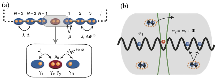
Figure 43: (Color online) (a) Schematics of the model Hamiltonian: the central part of the system is magnified in the box at the bottom, where the Majorana degrees of freedom included in the simplified model are highlighted. (b) Realization in a cold atom system. A 1D OL is coupled to a BEC reservoir that gives rise to the Kitaev Hamiltonian in the chain. An optical barrier acts both to create the impurity site (red) and triggers the Josephson effect in the reservoir itself. The phase difference across the barrier in the reservoir then acts as the phase $\Phi$ for the OL. Rrprinted by permission from Laflamme et al.[472].

Cold atom systems may provide a platform with high controllability to simulate and study the Kitaev chain model based on the remarkable advances in recent experiments. Several experimental proposals for realization of the Kitaev wires with cold atoms in the past years have been presented [473, 474, 475, 476, 477, 472], where the two key ingredients to induce the unpaired Majorana zero modes can be created. In these proposals, a single-piece gas of cold fermionic atoms which can be regarded as the spinless fermions are considered. Furthermore, the effective $p$-wave pairing term can be realized by a Raman induced dissociation of Cooper pairs [473] or Feshbach molecules [476] forming an atomic BCS (or BEC) reservoir. The Kitaev chain model is usually considered as a noninteracting system; however, the pairing in the superfluid should be formed in an interacting atomic system.

Without loss of generality, we describes a recent work for realizing the Kitaev wires with cold atoms [472]. In this experimental scheme, the model Hamiltonian describes the spinless fermions with field operator $\psi_{j}$ in a ring OL reads as [472]

$$H(\Phi) =\sum^{N-1}_{j=1}[-J\psi^{\dagger}_{j}\psi_{j+1}+\Delta\psi_{j}\psi_{j+1}-\frac{\mu}{2}(\psi^{\dagger}_{j}\psi_{j}-\frac{1}{2})]$$ (247)

$$+J_{L}\psi^{\dagger}_{N-1}\psi_{0}+J_{R}\psi^{\dagger}_{0}\psi_{1}e^{i\Phi/2}+\frac{\mu_{0}}{2}\psi^{\dagger}_{0}\psi_{0}+h.c.,$$

where $j=0,1...N-1$ labels the lattice sites. As shown in Fig. 43(a), it describes a proximity-induced $p$-wave superconductor with pairing $\Delta$, interrupted by an extra site at $j=0$ (assumed to be not affected by the pairing), $J$ and $\mu$ denote the normal nearest-neighbour hopping and the chemical potential relative to half-filling, respectively. The site at $j=0$ is connected to its neighbours by the hopping amplitudes $J_{L}$ and $J_{R}$, respectively, and has an energy offset $\mu_{0}$. The phase factor $e^{i\Phi/2}$ on the hopping between $j=0$ and $j=1$ represents the phase of a Cooper pair by $\Phi$ when moving around the ring. For $J_{L}=J_{R}=\mu_{0}=0$, the model Hamiltonian returns to the Eq. (228), which describes the original Kitaev chain model. Thus, for the case $|\mu|<2J$ and $|\Delta|>0$, the system hosts unpaired Majorana zero modes, $\gamma_{L}$ and $\gamma_{R}$, which are localized around $j=N-1$ and $j=1$, respectively.

In their proposed setup, three points to realize the model Hamiltonian are required: the realization of a 1D Kitaev chain, the additional single site separating the two ends of the chain, and the time control of the phase $\Phi$. A system of fermionic alkaline earth atoms prepared in their ${}^{1}S_{0}$ ground state in a 1D ring lattice was considered. The choice of alkaline earth atoms allows one to independently trap the ${}^{1}S_{0}$ ground state $|g\rangle$ and the ${}^{3}P_{0}$ metastable excited state $|e\rangle$. To address the first issue, the hopping terms $J$ in the lattice naturally arise and the pairing term $\Delta$ can be induced by coupling the fermions in the lattice to a BEC reservoir. Here a radio-frequency field is used to break up Cooper pairs into neighbouring sites directly in the lattice [473], as depicted in Fig. 43(b). The second step is to interrupt the chain with a single site. Following this idea, a barrier is engineered to inhibit $|g\rangle$ atoms from being at site $j=0$, which splits the Kitaev wire into two wires. It can be done by using a highly focused beam at the so-called anti-magic wavelength, which acts as a sink for $|e\rangle$, and as a source for $|g\rangle$. Consequently, the $|e\rangle$ atom only being trapped at site $j=0$ acts as the additional site coupling the two ends of the chain. Although the natural tunnelling into and out of this site is deterred by this barrier, the hopping $J_{L}$ and $J_{R}$ are then can be reintroduced with Raman processes involving a clock transition [114, 224, 478]. Finally, the realization of the time control of phase $\Phi$ is related to the Josephson effect where the additional site $j=0$ and its nearest-neighbour form a Josephson-like knot [472]. Within these setups, this system will occur a non-equilibrium Josephson effect with a characteristic $8\pi$ periodicity of the Josephson current. At this point, the system is pumped to an excited state after slowly increasing $\Phi$ by $4\pi$, and returns to the ground state after a second $4\pi$ cycle.

7.3 1D Anyon-Hubbard model

The Hubbard model of 1D lattice anyons with on-site interactions, called Anyon-Hubbard model, takes the form

$$H_{A}=-J\sum_{j=1}^{N}(a_{j}^{\dagger}a_{j+1}+h.c.)+U\sum_{j=1}^{N}n_{j}(n_{j}-1).$$ (248)

Here $n_{j}=a_{j}^{\dagger}a_{j}$ is the number operator for anyons and the operators $a_{j}$ and $a_{j}^{\dagger}$ annihilate or create an anyon on site $j$, and they are defined by the commutation relations

$$a_{j}a_{k}^{\dagger}-e^{-i\theta\text{sgn}(j-k)}a_{k}^{\dagger}a_{j}=\delta_{jk},\ \ \ a_{j}a_{k}=e^{i\theta\text{sgn}(j-k)}a_{k}a_{j},$$ (249)

which are parameterized by the statistical angle $\theta$. The sign function in the above equations is $\text{sgn}(j-k)=-1,0,1$ for $j<k$, $j=k$, $j>k$, respectively. Thus, two particles on the same site behave as ordinary bosons. Consequently, even for $\theta=\pi$, these lattice anyons are just pseudofermions: they are bosons on-site and fermions off-site, since many of them are allowed to occupy the same site.

There exists an exact mapping between anyons and bosons in 1D. Define the fractional version of a Jordan-Wigner transformation,

$$a_{j}=b_{j}\exp\left(i\theta\sum_{k=1}^{j-1}n_{k}\right),$$ (250)

with $n_{k}=a_{k}^{\dagger}a_{k}=b_{k}^{\dagger}b_{k}$ the number operator for both particle types. One can check that the mapped operators $a_{j}$ and $a^{\dagger}_{j}$ indeed obey the anyonic commutation relations in Eq. (249), provided that the particles of type $b$ are bosons with the bosonic commutation relations: $[b_{j},b_{k}^{\dagger}]=\delta_{jk}$ and $[b_{j},b_{k}]=0$. By inserting the anyon-boson mapping (250), the Hamiltonian (248) can be rewritten in terms of bosons [479],

$$H_{B}=-J\sum_{j=1}^{N}(b_{j}^{\dagger}b_{j+1}e^{i\theta n_{j}}+h.c.)+U\sum_{j=1}^{N}n_{j}(n_{j}-1).$$ (251)

Therefore, the anyonic exchange phase has been translated to an occupation-dependent Peierls phase: when tunneling from right to left $(j+1,j)$, a boson picks up a phase given by $\theta$ times the number of particles occupying the site that it jumps to. Under this condition, the many-body wave function picks up a phase of $\theta\ (-\theta)$ if two particles pass each other via two subsequent tunneling processes to the right (left). The proposed conditional-hopping scheme is depicted in Fig. 44. Interestingly, the non-local mapping between anyons and bosons in Eq. (250) leads to a purely local and thus realizable Hamiltonian (251).

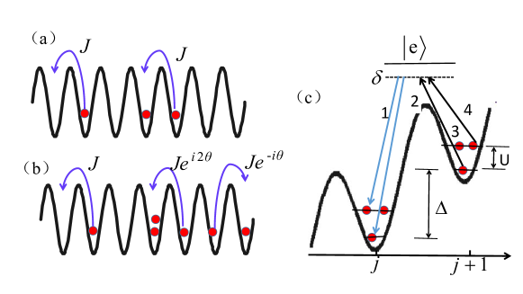
Figure 44: (Color online) The mapping between Anyon- and Boson-Hubbard models and a scheme to realize occupation-dependent gauge potential [479]. (a) Anyons in 1D can be mapped onto bosons featuring occupation-dependent gauge potential. (b) Assisted Raman tunnelling proposed for the realization of the Anyon-Hubbard model.

The occupation-dependent gauge potential can be implemented in OLs with a laser-assisted Raman tunneling scheme [479], generalized the idea proposed in Ref. [114] to create an artificial gauge potential, see the Sec.3.4.2. Figure (44) displays the basic concept. A non-zero on-site interaction $U$ is required to distinguish between different local occupational states. The OL is tilted, with an energy offset $\Delta$ between neighbouring sites. For simplicity, we consider lattice site occupations that are restricted to $n_{j}=0,1,2$, but higher local truncations are also possible. Two different occupational states in either of the two sites form in total a 4D atomic ground state manifold, which are coupled to an excited state $|e\rangle$ via four external driving fields, labelled $L_{1}$, $L_{2}$, $L_{3}$ and $L_{4}$ in Fig. 44(b).

The excited state can be experimentally realized in at least two alternative ways. First, two spin-dependent lattices can be used. We take ⁸⁷Rb as an example. One lattice traps atoms in the $F=1$, $m_{F}=-1$ hyperfine state, which is the ground state manifold. The $F=1$, $m_{F}=0$ hyperfine state is chosen as the excited state $|e\rangle$ and trapped in a second lattice. Atoms in the excited state would then be localized between the left and right wells of the $F=1$, $m_{F}=-1$ lattice, but not necessarily in their center. This implementation has the advantage of external driving fields in the radio-frequency regime. Such frequencies could resolve the typical energies $U$ and $\Delta$, both of the order of a few kHz, which requires a laser with a linewidth $\delta\ll U,\Delta$. This is a necessary condition for selectively coupling the four different states in the ground state manifold. Second, one can use two optical lattices, and trap ground state manifold atoms in the red-detuned lattice, while the excited state would live in the blue-detuned one. The driving fields required in this case would be typically in the THz frequency regime, making a precise resolution of $U$ and $\Delta$ more challenging in experiments.

The effective tunnelling rates $J_{ab}$ ($a\in{1,2}$, $b\in{3,4})$ between the four different levels are obtained in terms of the effective Rabi frequencies $J_{ab}=\Omega_{a}^{*}\Omega_{b}/\Delta$, where an overlap integral should be included in the Rabi frequencies $\Omega_{a,b}$ since ground and excited states feel different lattices. It is demonstrated that the model in Eq. (251) can be implemented if the conditions $J_{23}=J_{24}\equiv J$ and $J_{13}=J_{14}\equiv Je^{i\theta}$ were satisfied [479]. It is notable that the tilt energy $\Delta$ disappears in the effective Hamiltonian after rotating out time-dependent phase factors, this energy offset is absorbed by the external radiation field, yielding a total Hamiltonian without a tilt term.

To realize the model in Eq. (251), one has the parameters to satisfy the following conditions. (i) The lasers linewidth $\delta\ll\Delta,U$, so that the external driving fields can resolve the different levels of the ground state manifold. (ii) A short-lived excited state and the validity of the adiabatic elimination require large detunings $\Delta\gg|\Omega_{1-4}|$. (iii) $\Delta$ and $U$ can be in the same frequency regime (a few kHz), but their difference should be much larger than the lasers linewidth $\delta$. As an example, $\Delta\approx 2$ kHz, $U\approx 3$ kHz, $|J_{ab}|=J\approx 5$ kHz and $|\Omega_{ab}|\approx 20$ kHz would be sufficient if the linewidth of the radiation field were $\delta\approx 50$ Hz, which is a realistic assumption for typical radio-frequency driving fields. However, it was shown in Ref. [480] that a further condition $U,\Delta\gg\delta$ is also required in the above scheme. For typical experimental parameters, it would lead to large heating. This drawback was solved by a scheme proposed in Ref. [480], where one ground-state component bosonic gas is replaced by two ground-state components atomic gas.

An alternative scheme for the experimental realization of 1D Anyon-Hubbard model, based on time-periodic forcing, was proposed in Ref. [481]. The occupation-dependent Peierls phase can be engineered by means of coherent lattice-shaking-assisted tunneling against potential offsets created by a combination of a static potential tilt and strong on-site interaction. The potential tilt $\Delta$ is added in the Hamiltonian with the term $\Delta jb_{j}^{\dagger}b_{j}$. By shaking the lattice, a similar term $F(t)jb_{j}^{\dagger}b_{j}$ can be further added in the Hamiltonian, where $F(t)=F(t+T)$ incorporates a homogeneous time-periodic force of angular frequency $\omega=2\pi/T$ with vanishing cycle average $1/T\int_{0}^{T}dtF(t)=0$ and the resonance condition $\Delta=\hbar\omega$. It can be implemented as an inertial force $F(t)/a=-m\ddot{x}(t)$, with lattice constant $a$, by shaking the lattice $x(t)$ back and forth.

A fully 1D Anyon-Hubbard model introduced here has not yet been experimentally realized. However, some relevant ingredients have been achieved, such as the experimental implementation of tunable occupation-dependent tunneling with Floquet engineering of the on-site interaction energy [482] and the realization of the occupation-number sensitivity of the tunneling [483]. These techniques may immediately applied to generating low-dimensional anyons.

7.4 Bosonic quantum Hall states

The integer and fractional QHE are among the most important discoveries in condensed matter physics in 1980s. It is a quantum-mechanical version of the Hall effect, observed in 2D electron systems subjected to low temperatures and strong magnetic fields, in which the Hall conductance $\sigma_{H}$ undergoes quantum Hall transitions to take on the quantized values $\sigma_{H}=\nu\frac{e^{2}}{h}$, where $e$ is the elementary charge and $h$ is Planck’s constant. The prefactor $\nu$ is known as the filling factor, and can take on either integer or fractional values. The QHE is referred to as the integer or fractional QHE depending on whether $\nu$ is an integer or fraction, respectively. Until now, the QHE has been observed only in electron systems. Can we experimentally observe such important quantum properties in other systems is still a long-standing open question. Recently, there has been considerable progress towards their realization in cold-atom systems. In this section, we introduce several theoretical proposals for realization of the QHE with cold atoms. In principle, both bosonic and fermionic atoms can be used in the experiments; however, the preparation of topological states of matter relies on quick thermalization and cooling below the many-body gap, which is hard to achieve in cold atom systems. Since bosonic atoms are generally easier to cool, we focus on the realization of the QHE with bosonic atoms. We will mainly focus on the realizations of bosonic integer QHE with a Chern number $C=2$, and the fractional quantum Hall state with the filling factor $\nu=1/2$, since they will be the most experimentally accessible conditions.

Compared with the QHE of fermions, non-interacting boson phases are topologically trivial, and integer QHE with bosons can only occur under the strong interactions. The needed strong interactions for creating bosonic quantum Hall states makes them harder to study than their fermionic cousins. As a smoking gun of the realization of quantum Hall state, one can compute the many-body Chern number of the ground state $|\Psi\rangle$. In the theory of the QHE, it is well understood that the conductance quantization is due to the existence of certain topological invariants, the so-called Chern numbers. The Chern numbers with the single-particle problem and Bloch waves have been introduced in the previous sections. For fermions, the Chern number is defined as an integration over the occupied states in momentum space [10]. This definition cannot be applied to the bosonic system as many bosons can occupy the same momentum state. The generalization to many-body systems has been proposed by Niu et al. [484] by manipulating the phases under the closed boundary conditions on a torus for both the integer and fractional quantum Hall systems. Suppose the ground state $|\Psi\rangle$ has a gap to the excited state and depends on the parameters $\theta_{x},\theta_{y}$ through the generalized periodic boundary conditions:

$$|\Psi(m+M,l)\rangle=e^{i\theta_{x}}|\Psi(m,l)\rangle,\ \ \ |\Psi(m,l+L)\rangle=e^{i\theta_{y}}|\Psi(m,l)\rangle,$$

where $M\times L$ denotes the system size, and $(\theta_{x},\theta_{y})$ are the twist angles vary on the torus. Under this boundary condition, we numerically diagonalize the Hamiltonian of the system and derive the ground state $|\Psi(\theta_{x},\theta_{y})\rangle$, and then one can define the many-body Chern number $C_{\text{MB}}$ as a topological invariant by the following formula [484]

$$C_{\text{MB}}=\frac{1}{2\pi}\int_{0}^{2\pi}d\theta_{x}\int_{0}^{2\pi}d\theta_{y}(\partial_{\theta_{x}}A_{\theta_{y}}-\partial_{\theta_{y}}A_{\theta_{x}}),$$ (252)

where the Berry connection $A_{\mu}\equiv i\langle\Psi(\theta_{x},\theta_{y})|\partial_{\mu}|\Psi(\theta_{x},\theta_{y})\rangle$ $(\mu=\theta_{x},\theta_{y})$.

As for fractional quantum Hall state, one can also calculate the overlap between the ground state and the Laughlin wavefunction. If $N$ is the number of particles in the system and $N_{\phi}$ is the number of magnetic fluxes measured in units of the fundamental flux quanta $\Phi_{0}=2\pi\hbar/e$, we can define the filling factor $\nu=N/N_{\phi}$. In the simplest form the fractional QHE occurs if the number of magnetic fluxes is an integer $1/\nu$. At this value of the magnetic field, the ground state of the system is an incompressible quantum liquid which is separated from all other states by an energy gap and is well described by the Laughlin wavefunction

$$\Psi({z}_{1},{z}_{2},\dots z_{N})=e^{-\sum_{j}|{z}_{j}|^{2}/4}\prod_{j<k}({z}_{j}-{z}_{k})^{1/\nu},$$ (253)

where $z=x+iy$. Due to the Pauli principle, only the states with odd (even) $1/\nu$ is applicable to fermions (bosons). In the following, we will address bosonic QHE in both single- and two-component Bose-Hubbard models.

7.4.1 Single-component Bose-Hubbard model

We consider single-component bosonic atoms at zero temperature confined in a 2D square OL with the lattice constant $a$ and a background harmonic potential in the presence of artificial magnetic field. In the Landau gauge, the system is well described by the Bose-Hubbard model with Peierls substitution term in the nearest-neighbor hopping,

$$H=\sum_{m,l}\left[-J\left(e^{i2\pi\alpha l}b^{\dagger}_{m+1,l}b_{m,l}+b^{\dagger}_{m,l+1}b_{m,l}+h.c.\right)+\frac{U}{2}\hat{n}_{m,l}(\hat{n}_{m,l}-1)-(\mu-V_{m,l})\hat{n}_{m,l}\right],$$ (254)

where $J$ is the hopping energy between two neighboring sites, $U$ is the on-site interaction energy, and the phase $2\pi\alpha$ arises from the artificial magnetic field and $0\leq\alpha\leq 1$ is the flux quanta per plaquette. $\mu-V_{m,l}$ is the local chemical potential with $V_{m,l}$ being the trapping potential. In the Bose-Hubbard Hamiltonian, the hopping and on-site interaction are the two competing terms, and both of them can be tuned over a wide range of values by changing the depth of the lattice potential and employing Feshbach resonance. The phase diagram of the Bose-Hubbard model for $\alpha=0$ is well-known: the Mott-insulator phase corresponds to the strong on-site interaction limit $J/U\ll 1$, and superfluid phase corresponds to the opposite limit $J/U\gg 1$.

It was first proposed in Ref. [122] that fractional quantum Hall states may occur in the single-component Bose-Hubbard model. They argued that the interactions of atoms localized in the lattices are strongly enhanced compared to the interaction of atoms in free space, so the created states of the quantum Hall type in OLs are characterized by large energy gaps. It is a clear advantage from an experimental point of view because the state is more robust against external perturbations. There are two energy scales for the system in the presence of an artificial magnetic field: the first is the magnetic tunneling term, $J\alpha$, which is related to the cyclotron energy in the continuum limit $\hbar\omega_{c}=4\pi J\alpha$, and the second is the on-site interaction energy $U$. By using the method of exact diagonalization [122], it was shown that the overlap of the ground state wave function $|\Psi\rangle$ of the Hamiltonian in Eq. (254) with the Laughlin wave function is very good when $\nu=1/2$ for $\alpha\leq 0.3$, but the overlap start to fall off for $\alpha\geq 0.3$. Furthermore, the Chern numbers for fixed $\nu=1/2$ and different $\alpha$’s were calculated in Ref. [485]. The results show that, for higher $\alpha$, the lattice structure becomes more apparent and the overlap with the Laughlin state decreases. However, the ground state remains twofold degenerate and the ground state Chern number tends to remain equal to 1 before reaching some critical $\alpha_{c}\approx 0.4$.

The states in the Bose-Hubbard model can be classified based on the compressibility defined by $\kappa=\partial\rho/\partial\mu$, where the density $\rho=\sum_{m,l}\langle\Psi|\hat{n}_{m,l}|\Psi\rangle/(ML)$. It is incompressible ($\kappa=0$) for the quantum Hall states, and finite for the superfluid states. The compressibility of the Hamiltonian in Eq. (254) was calculated by using the cluster Gutzwiller mean field theory in Ref. [486]. The results for $\alpha=1/5$ and $\alpha=1/2$ are plotted in Fig. 45. The states in superfluid phase are compressible, as a result, the density $\rho$ varies linearly with the chemical potential $\mu$. However, for specific values of filling factor $\nu$ there are states with constant $\rho$, represented by the blue horizontal lines, and these incompressible positions correspond to the existence of quantum Hall states. In Fig. 45(a), the plateaus or the constant $\rho$ values correspond to $\nu=1/2,1,3/2,2,5/2,3,7/2,4,9/2$ and the corresponding $\rho$ values are $\nu\alpha$. In Fig. 45(b), the plateaus correspond to $\nu=1/2,1,3/2$.

Whether a state with integer filling factor in Fig. 45 is an integer quantum Hall state should be carefully analyzed. It was demonstrated that the conductivity $\sigma_{xy}$ must be even for any bosonic quantum Hall state without fractional quasiparticle excitations [487]. To have a basic idea about this issue, we consider some excitations created in a general bosonic quantum Hall state. Each of them can be considered as a bosonic particle attaching with $2\pi$ flux and has charge $\sigma_{xy}$. If we braid one excitation around another, the statistical phase follows from the Aharonov-Bohm effect: $\theta=2\pi\sigma_{xy}$. Similarly, if we exchange two excitations, the associated phase is $\theta/2=\pi\sigma_{xy}$. On the other hand, if the state does not support fractional quasiparticles, then these excitations must be bosons. Therefore, we conclude that $\sigma_{xy}$ must be even for any bosonic quantum Hall state without fractional quasiparticle excitations. Based on this argument, the $\nu=1$ state in Fig. 45(a) cannot be a stable integer quantum Hall state.

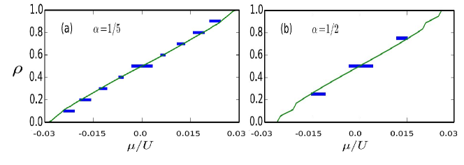
Figure 45: (Color online) The variation in the number density $\rho$ in the presence of an artificial magnetic field with $\alpha=1/5$ in (a) and for $\alpha=1/2$ in (b). The states in superfluid are compressible and $\rho$ varies linearly with $\mu$, as shown with solid black lines. For specific values of filling factor $\nu$ there are states with constant $\rho$, represented by the blue lines, and these incompressible states correspond to the existence of quantum Hall states. Reprinted with permission from Bai et al.[486]. Copyright© (2018) by the American Physical Society.

Notably, the integer quantum Hall state for single component bosons can occur in some lattice structures with Chern number $C_{\text{MB}}=2$ [488, 489, 490, 491]. Recently, two different lattice versions of bosonic quantum Hall states have been proposed at integer filling $\nu=1$ of the lowest topological flat-band with $C_{\text{MB}}=2$. The optical flux lattice has been studied by exact diagonalization of the projected Hamiltonian in momentum space [490] and correlated Haldane honeycomb lattice has been studied by infinite density matrix renormalization group of hardcore boson in real space. The authors in Ref. [489] established the existences of the bosonic quantum Hall phase in their model by providing numerical evidence: (i) a quantized Hall conductance with $\sigma_{xy}=2$; (ii) two counter propagating gapless edge modes. On the other hand, it was demonstrated that bosonic integer quantum Hall state emerges in integer boson filling factor $\nu=1$ of the lowest band in a generalized Hofstadter lattice (including the nearest neighbor hopping) with $C_{\text{MB}}=2$ [488].

7.4.2 Two-component Bose-Hubbard model

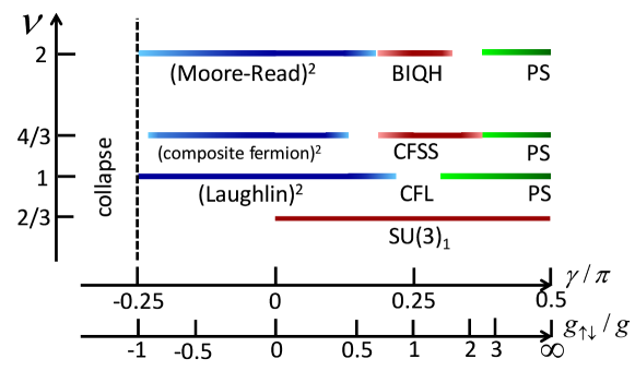
Figure 46: (Color online) Ground-state phase diagram in the space of the total filling factor $\nu$ and the ratio $U_{\uparrow\downarrow}/U=\tan\gamma$ between the intercomponent coupling constant and the intracomponent one. The product states of a pair of nearly uncorrelated quantum Hall states (Laughlin, composite fermion, and Moore-Read states) appear when $U_{\uparrow\downarrow}<0$. BIQH: bosonic integer quantum Hall state; PS: phase separation; CFSS:composite fermion spin-singlet state; CFL: composite fermion liquid. $SU(3)_{1}$: the Halperin state with an $SU(3)_{1}$ symmetry. Reprinted with permission from Furukawa et al. [492]. Copyright© (2017) by the American Physical Society.

We further address the quantum Hall states in a two-component Bose-Hubbard model. We consider a system of a 2D pseudospin-1/2 bosonic gas (in the $xy$ plane) subject to the same magnetic fields $B$ along the $z$ axis for both spin states. In the second-quantized form, the interaction Hamiltonian is written as

$$H_{\text{int}}=\sum_{\alpha\beta}\frac{U_{\alpha\beta}}{2}\int d^{2}\mathbf{r}\hat{\Psi}_{\alpha}^{\dagger}(\mathbf{r})\hat{\Psi}_{\beta}^{\dagger}(\mathbf{r})\hat{\Psi}_{\alpha}(\mathbf{r})\hat{\Psi}_{\beta}(\mathbf{r}),$$

where $\hat{\Psi}_{\alpha}(\mathbf{r})$ is the bosonic field operator for the spin state $\alpha$ ($=\uparrow$ or $\downarrow$). We set the strengths of the intracomponent contact interactions $U_{\uparrow\uparrow}=U_{\downarrow\downarrow}=U>0$ and the strengths of the intercomponent contact interactions $U_{\uparrow\downarrow}=U_{\downarrow\uparrow}$. For a 2D system of area A, the number of magnetic flux quanta piercing each component is given by $N_{\phi}=|\phi|/(2\pi\hbar)=A/(2\ell^{2})$, where $\ell=\sqrt{\hbar A/|\phi|}$ is the magnetic length. Strongly correlated physics is expected to emerge when $N_{\phi}$ becomes comparable with or larger than the total number of particles, $N=N_{\uparrow}+N_{\downarrow}$, where $N_{\uparrow}$ and $N_{\downarrow}$ are the numbers of pseudospin-$\uparrow$ and $\downarrow$ bosons, respectively.

The ground-state phase diagram of pseudospin-1/2 bosonic gases in a uniform artificial magnetic field in the space of the total filling factor $\nu=N/N_{\phi}$ and the coupling ratio $U_{\uparrow\downarrow}/U$ were numerically calculated by performing an extensive exact diagonalization analysis in the lowest-Landau level based on spherical and torus geometries [492]. The main results are summarized in Fig. 46. In the figure, the two coupling constants are parametrized as

$$(U,U_{\uparrow\downarrow})=G\ell^{2}(\text{cos}\gamma,\text{sin}\gamma),$$

where $G>0$, and $\gamma\in[-\pi/2,\pi/2]$. As can be seen in this diagram, when the intercomponent coupling is attractive ($U_{\uparrow\downarrow}<0$), doubled quantum Hall states are remarkably robust and persist even when $|U_{\uparrow\downarrow}|$ is comparable to the intracomponent coupling $U$. This sharply contrasts with the case of an intercomponent repulsion ($U_{\uparrow\downarrow}<0$), where a variety of spin-singlet quantum Hall states with high intercomponent entanglement emerge for $U_{\uparrow\downarrow}\approx U$. This remarkable dependence on the sign of $U_{\uparrow\downarrow}$ can be interpreted in light of Haldane s pseudopotentials on a sphere. More specifically, the stability of the doubled quantum Hall states for $U_{\uparrow\downarrow}<0$ can be understood from the ferromagnetic nature of the intercomponent interaction in terms of (modified) angular momenta of particles. Meanwhile, various spin-singlet quantum Hall states with a finite excitation gap emerge for pseudospin-independent [$SU(2)$-symmetric] interactions with $U_{\uparrow\downarrow}=U$. Among those states, relatively large gaps are found for the Halperin state with an $SU(3)_{1}$ symmetry at $\nu=2/3$ [493] and a bosonic integer quantum Hall state protected by a $U(1)$ symmetry at $\nu=2$ [487, 494]. At $\nu=4/3$, two types of spin-singlet quantum Hall states compete in finite-size systems: a non-Abelian $SU(3)_{2}$ state and a composite fermion spin-singlet state. Furthermore, a gapless spin-singlet composite Fermi liquid has been shown to appear at $\nu=1$ [495]. In all these spin-singlet states, the two components are highly entangled. For small $U_{\uparrow\downarrow}/U$, in contrast, the system can be viewed as two weakly coupled scalar bosonic gases, and the product states of nearly independent quantum Hall states (doubled quantum Hall states) are expected to appear.

We can compare the phase diagram in Fig. 46 with that of the two-component bosonic gases in antiparallel magnetic fields [496]. In the latter case, the pseudospin $\uparrow$ ($\downarrow$) component is subject to the magnetic field $B$ $(-B)$ in the direction perpendicular to the 2D gas, and the system possesses the TRS [84, 108]. In the regime with $\nu=O(1)$, (fractional) quantum spin Hall states [21] composed of a pair of quantum Hall states with opposite chiralities are robust for an intercomponent repulsion $U_{\uparrow\downarrow}>0$ and persist for $U_{\uparrow\downarrow}$ as large as $U$. Similar results have also been found in the stability of two coupled bosonic Laughlin states in lattice models. These results suggest that the case of $U_{\uparrow\downarrow}>0$ for antiparallel fields essentially corresponds to the case of $U_{\uparrow\downarrow}<0$ for parallel fields [492].

7.5 Kitaev honeycomb model

Generalized the previous idea on realization of the unpaired Majorana zero modes in a 1D system, in 2006, Kitaev further proposed another model that unpaired zero-energy Majorana modes can appear in a 2D spin-1/2 system on a honeycomb lattice, where nearest-neighbor interactions can be reduced to a problem of non-interacting Majorana fermions [497]. It is one of the rare examples where a complex system is described by an exactly solvable 2D spin Hamiltonian. Its quantum-mechanical ground state is a quantum spin liquid and supports exotic excitations which obey Abelian or non-Abelian statistics.

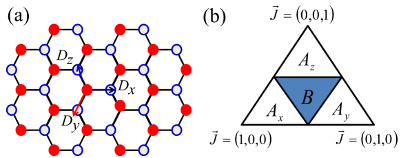
Figure 47: (Color online) (a) Kitaev model on the honeycomb lattice where interactions between nearest neighbors are $J_{\nu}$, depending on the direction of the link $D_{\nu}$. (b) The phase diagram of the Kitaev honeycomb model in the $J_{x}+J_{y}+J_{z}=1$ plane in the parameter space. In the three unshaded areas labeled $A_{x}$, $A_{y}$, and $A_{z}$, the system is gapped with Abelian anyon excitations, and in the shaded area labeled $B$ the system is gapless with non-Abelian excitations.

The Kitaev honeycomb model is a spin-1/2 system in which spins are located at the vertices of a honeycomb lattice with a spatially anisotropic interaction between neighboring spins, as shown in Fig. 47(a). This lattice consists of two equivalent sublattices labelled ‘A’ and ‘B’, which are shown by open and filled circles. A unit cell of the lattice contains both of them. The Hamiltonian is given by [497]

$$H_{\text{KHM}}=-\sum_{\nu,\langle j,l\rangle\in D_{\nu}}J_{\nu}\sigma^{\nu}_{j}\sigma^{\nu}_{l},$$ (255)

where $\sigma^{\nu}_{j}$ are the Pauli matrices at the site $j$, $J_{\nu}$ ($\nu=x,y,z$) are interaction parameters, and the symbol $\langle j,l\rangle\in D_{\nu}$ denotes the neighboring spins in the $D_{\nu}$ directions. Neighboring spins in Heisenberg models normally interact isotropically so that the spin-spin interaction does not depend on the spatial direction between neighbors. In the above model, however, neighboring spins along links pointing in different directions interact differently.

The ground state of the Kitaev honeycomb model has two distinct phases in the parameter space and the phase diagram can be shown in terms of points in an equilateral triangle satisfying $J_{x}+J_{y}+J_{z}=1$ (the value of $J_{\nu}$ is the distance from the opposite side), as shown in Fig. 47(b) [497]. If $J_{x}<J_{y}+J_{z}$, $J_{y}<J_{z}+J_{x}$ and $J_{z}<J_{x}+J_{y}$, the system is gapless with non-Abelian excitations corresponding to $B$ phase. For all other values of $(J_{x},J_{y},J_{z})$, the system is gapped with Abelian anyon excitations, labelled, $A_{x}$ where $J_{x}>J_{y}+J_{z}$, $A_{y}$ where $J_{y}>J_{z}+J_{x}$, $A_{z}$ where $J_{z}>J_{x}+J_{y}$. The gapped phases, $A_{x}$, $A_{y}$, and $A_{z}$, are algebraically distinct, though related to each other by rotational symmetry. They differ in the way lattice translations act on anyonic states, and thus a continuous transition from one gapped phase to another is impossible. The two phases $A$ and $B$ are separated by three transition lines, i.e., $J_{x}=1/2$, $J_{y}=1/2$, and $J_{z}=1/2$, which form a small triangle in the $B$ phase.

Precise proposals to realize an artificial Kitaev model using atomic OLs have been made in the literature [435, 498], where the well-controllable OLs offer the possibility of designing such anisotropic spin lattice models. The main idea is that the two-component Bose-Hubbard model in a honeycomb lattice can reduce to the Kitaev spin model at half filling and large on-site repulsion. For completeness, we here focus on the proposal in Ref. [435] and its modified implementation scheme for ⁸⁷Rb atoms proposed in Ref. [498]. To implement the Kitaev honeycomb model using ultracold atoms, we first get an effective 2D configuration with a set of independent identical 2D lattice in the $xy$ plane by raising the potential barriers along the vertical direction $z$ in the 3D OL so that the tunneling and the spin exchange interactions in $z$ direction are completely suppressed. And then a honeycomb lattice can be constructed with three trapping potentials of the forms

$$V_{j}(x,y)=V_{0}\text{sin}^{2}[k_{\parallel}(x\text{cos}\theta_{j}+y\text{sin}\theta_{j}+\varphi_{0}),$$ (256)

where $j=1,2,3$, and $\theta_{1}=\pi/6$, $\theta_{2}=\pi/2$, $\theta_{3}=-\pi/6$. Each of the potentials is formed by two blue-detuned interfering traveling laser beams above the $xy$ plane with an angle $\varphi_{\parallel}$, so that the wave vector $k_{\parallel}$ projected onto the $xy$ plane has the value $k_{\parallel}=k\text{sin}(\varphi_{\parallel}/2)=k/\sqrt{3}$. The relative phase $\varphi_{0}$ is chosen as $\pi/2$ in Eq. (256) so that the maxima of the three potentials overlap. In this case, the atoms are trapped at the minima of the potentials and the potential barrier between neighboring atoms is around $V_{b}\approx V_{0}/4$. Actually, the honeycomb (hexagonal) lattice and its topologically equivalent configuration, the brick wall lattice, have been experimentally realized by several groups [77, 28, 140]. We consider a ⁸⁷Rb BEC and two hyperfine ground states $|\uparrow\rangle=|F=2,m_{F}=-2\rangle$ and $|\downarrow\rangle=|F=1,m_{F}=-1\rangle$ are defined as the effective atomic spin. The potential barrier between neighboring atoms in the honeycomb lattice is adiabatically ramped up to approximately $V_{b}=14E_{R}$ to obtain a Mott insulator state with one atom per lattice site, where $E_{R}=\hbar^{2}k^{2}/(2m)$ is the recoil energy for Rb atoms.

In this hexagonal lattice, one can engineer the anisotropic spin-spin interactions $J_{\nu}\sigma_{j}^{\nu}\sigma_{m}^{\nu}$ in Eq. (255) using additional spin-dependent standing wave laser beams in the $xy$ plane. To this end, one can apply three blue-detuned standing-wave laser beams in the $xy$ plane along the tunneling directions denoted by $D_{x}$, $D_{y}$, and $D_{z}$, respectively:

$$V_{\nu\sigma}(x,y)=V_{\nu\sigma}\text{sin}^{2}[k(x\text{cos}\chi_{\nu}+y\text{sin}\chi_{\nu}),$$ (257)

where $\chi_{x}=-\pi/3$, $\chi_{y}=\pi$, $\chi_{z}=\pi/3$. With properly chosen laser configurations, a spin-dependent potential

$$V_{\nu\sigma}=V_{\nu+}|+\rangle_{\nu}\langle+|+V_{\nu-}|-\rangle_{\nu}\langle-|$$ (258)

along different tunneling directions $\nu$ can be generated, where $|+\rangle_{\nu}$ ($|-\rangle_{\nu}$) is the eigenstate of the corresponding Pauli operator $\sigma^{\nu}$ with the eigenvalue $+1(-1)$. One can adjust $V_{+}^{\nu}$ and $V_{-}^{\nu}$ by varying the laser intensity in the $D_{\nu}$ direction so that atoms can virtually tunnel with a rate $t_{+\nu}$ only when it is in the eigenstate $|+\rangle_{\nu}$, which yields the effective spin-spin exchange interactions $J_{\nu}\sigma_{j}^{\nu}\sigma_{m}^{\nu}$ with the interaction strength $J_{\nu}\approx-t^{2}_{+\nu}/(2U)$. Here the on-site interactions $U_{\uparrow\downarrow}\approx U_{\uparrow}\approx U_{\downarrow}\approx U$.

As for a typical example, we introduce more detailed on how to generate the spin-spin interaction $J_{z}\sigma_{j}^{z}\sigma_{m}^{z}$ in the Hamiltonian Eq. (255) following the proposal in Ref. [498], and the other spin-spin interaction terms can be created using a similar procedure [435]. The potentials (257) and (258) do not have influence on the equilibrium positions of the atoms, but they change the potential barrier between the neighboring atoms in the $D_{z}$ direction from $V_{b}\approx V_{0}/4$ to $V_{z\sigma}^{\prime}=V_{b}+V_{z\sigma}$. The standing wave laser beam used for generating spin-dependent tunneling is along the $z$-link direction and has a detuning $\Delta_{0}=2\pi\times 3600$ GHz to the $5^{2}P_{3/2}$ state (corresponding to a wavelength $787.6$ nm). This laser beam forms a blue-detuning potential for atoms with spin $|\uparrow\rangle$, but a red-detuning potential for $|\downarrow\rangle$ atoms. For instance, with a properly chosen laser intensity, the spin-dependent potential barriers may be set as $V_{\downarrow}=8E_{R}$ and $V_{\uparrow}=-4E_{R}$, which, combined with the spin-independent lattice potential barrier $V_{0}=14E_{R}$, yield the total effective spin-dependent lattice potential barriers $V_{\downarrow}=22E_{R}$ and $V_{\uparrow}=10E_{R}$ for neighboring atoms in the honeycomb lattice. Therefore, the tunneling rates for two spin states satisfy $t_{\uparrow}/t_{\downarrow}\gg 1$, which leads to the spin-spin interaction $J_{z}\sigma_{j}^{z}\sigma_{m}^{z}$ with $J_{z}\approx t^{2}_{\uparrow}/U$, as shown in Ref. [435]. For ⁸⁷Rb atoms, the time scale for the spin-spin interaction $h/J_{z}\approx$ 10 ms. By carefully tuning the spin-dependent lattice depth in different directions, one can in principle access all phases of the Kitaev honeycomb model. However, to observe the properties in this model, the temperature of the system needs to be much lower than the spin-spin interaction strength $T\ll J_{z}/k_{B}\approx 1$ nK, which sets a strict requirement for experiments. Higher temperatures will populate the system with an excess of unwanted excitations.

The Kitaev honeycomb model is an exactly soluble spin model that carries excitations with both Abelian and non-Abelian anyonic braiding statistics, which are the hallmarks of topological quantum matter. The advantage of the realization of this model with OLs is that both the Abelian and non-Abelian phases can be accessed just by varying the OL parameters. On the other hand, how to create, braid, and detect these anyons in this spin model defined on a honeycomb OL have also been proposed in Ref. [498], which is an important first step towards topological quantum computation. Furthermore, even the simple observation of Abelian anyonic properties in an OL and the subsequent read-out them will be a break-through achievement in itself, because anyonic statistic has never been directly demonstrated in any experimental system.

8 Conclusion and outlook

In the previous sections, we have reviewed the recent theoretical and experimental advances on exploring topological quantum matter with cold atoms. The cold atom systems provide many interesting possibilities of searching for exotic topological states that are currently absent or unrealizable in real materials. These include some unconventional topological insulators and semimetals, the topological phases with many-body interactions, non-equilibrium dynamics, and non-Hermitian or dissipation perturbations. So far, the theoretical understanding of these phases is limited and most experimental studies are at the single-particle level, but progress is already being made. In this final section of the review, we aim to discuss some promising developments for the near future.

8.1 Unconventional topological bands

Ultracold atomic gases in OLs with fully engineered geometries and atomic hopping forms provide a promising platform for exploring certain unconventional topological bands. These include some unconventional topological insulators and semimetals that are difficult to realize in solid-state materials, such as the chiral topological insulators protected by the chiral symmetry [308, 309, 163], topological nodal-line semimetals protected by the combined space-time symmetry [285, 292], and the topological bands with unconventional relativistic quasiparticles [350, 355, 358]. The chiral symmetry played by certain sublattice symmetry is typically broken by disorder potential in real materials; however, it naturally arises for cold atoms in OLs with negligible disorder [309]. The topological semimetals or metals with tunable structures of nodal points or lines could be experimentally implemented by varying the atom-laser interaction configuration [355, 499].

Furthermore, some theoretically predicted topological insulators beyond the ten-fold classification could be implemented in OLs. These include the Hopf insulators [66, 314, 317], the 3D quantum Hall states [265], the topological crystalline insulators stabilized by crystalline lattice symmetries [500], the topological Anderson insulators [501, 502, 503], and the so-called higher-order topological insulators and semimetals [504, 505, 506, 507, 508, 509]. The topological Anderson insulator is a disorder-driven topological phase, where the static disorder induces nontrivial topology when added to a trivial band structure [501, 502, 503]. Although there are many theoretical studies, the topological Anderson insulator has so far evaded experimental realization due to the lack of precise control over disorder and topology in real materials. In a recent experiment, evidence for the topological Anderson insulator phase in synthetic cold-atomic wires with controllable disorder has been found [349]. As an extension of the topological insulator family, the recently proposed higher-order ($n$-th order) topological insulators can host quantized multipole moments in the bulk bands, such as quadrupole and octupole, and has robust gapless states at the intersection of $n$ crystal faces (but is gapped otherwise). For instance, a bulk 2D topological quadrupole insulator described by nested Wilson loops hosts protected corner states with fractional charges [504], and its extension to a layered 3D system can give rise to a topological quadrupolar semimetal [509]. It was also proposed to realize topological quadrupole insulators using ultracold atoms in an optical superlattice [504].

Cold gases also allow the exploration of band topology in $D=d_{r}+d_{s}$ dimensions higher than the real dimension $d_{r}=3$, through the use of $d_{s}$ synthetic dimensions. A recent experiment has demonstrated the topological response of an effective 4D system by using 2D pumping in an OL [17]. Other topological states in 4D would be studied in the near future, such as 4D intriguing fractional phases induced by interactions [16] and time-reversal-symmetric 4D QHE. In addition, the 5D generalization of the topological Weyl semimetals with Yang monopoles and linked Weyl surfaces in the BZ [510, 511] would be similarly simulated with cold atoms. Very recently, the quantum simulation of a Yang monopole in a 5D parameter space built from the internal states of an atomic quantum gas was reported [512]. Moreover, its topological charges (the second Chern numbers) were measured by experimentally characterizing the associated non-Abelian Berry curvatures in the parameter space.

8.2 Other interacting topological phases

Topological superfluids with Majorana bound states. It has been theoretically shown that the $p+ip$-wave or $p$-wave topological superconductors/superfluids can be effectively induced in conventional $s$-wave superconductors/superfluids by combining the SOC and Zeeman splitting [513, 514, 515, 516]. The zero-energy Majorana bound states with non-Abelian statistics can emerge in these systems, but they have not yet been experimentally confirmed. With the recent advances, all the individual ingredients including the synthetic SOC and effective Zeeman fields for topological superfluids in fermionic quantum gases are in place. Several concrete proposals for realizing exotic topological superfluids with Majorana bound states for cold atomic gases have been proposed [514, 515, 516, 517, 103, 473, 518, 519]. Recently, a 2D SOC and a perpendicular Zeeman field have been simultaneously generated in ultracold Fermi gases [35, 113], which paved the way for future exploration of topological superfluids in ultracold atoms. Once the systems are experimentally realized, the high degree of experimental control over these cold atom systems will enable new approaches for the direct observation and manipulation of Majorana bound states, such as non-Abelian braiding.

Topological Mott insulators. In general, a strong interaction will open a trivial energy gap and break the band topology. However, there exists a class of topological insulators called the topological Mott insulators [520], where the many-body interactions are responsible for topological insulator behaviors. Although the topological Mott insulator phase was first reveled in an extended Fermi-Hubbard model on a 2D honeycomb lattice [520], it has now been known as a class of interaction-induced topological insulators for interacting fermions or bosons. The topological Mott insulators in 1D and 3D fermion systems have also been investigated [521, 522, 523]. Whereas many studies provide growing evidence for the existence of the topological Mott insulating phase, its experimental observation in electron systems is still outstanding. The schemes for realizing the topological Mott insulator with Rydberg-dressed fermionic atoms in 2D OLs were put forward [524, 525]. Furthermore, several works have theoretically and numerically shown that the topological Mott insulator phase can occur for interacting bosonic atoms [189, 526, 527, 528], atomic mixtures [529], and fermionic atoms [530] in 1D optical superlattices. Due to the tunable atomic interactions in OLs (similar as the engineered Bose- or Fermi-Hubbard models for cold atoms), these artificial systems may provide the first realization of topological Mott insulators in the near future.

Topological Kondo insulators. A class of topological insulators called topological Kondo insulators for few heavy-fermion materials were recently predicted [531, 532, 533], which originates from the hybridization between itinerant conduction bands and correlated electrons. Topological Kondo insulators are essentially induced by the strongly correlated Kondo effect that leads to the insulating gap, although they share the same topological properties with conventional topological insulators. Little evidence for a topological Kondo insulator state in SmB₆ has been reported [534, 535], and more theoretical and experimental works are needed to fully understand it. On the other hand, a scheme has recently been proposed to realize and observe topological (Chern) Kondo insulators in a 2D optical superlattice with laser-assisted $s$ and $p$ orbital hybridization and a synthetic gauge field [536]. The topological Kondo insulator phase was also predicted on interacting “sp-ladder” models [537, 538], which could be experimentally realized in OLs with higher orbitals loaded with ultracold fermionic atoms. Motivated by experimental advances on ultracold atoms coupled to a pumped optical cavity [539], a scheme for synthesizing and observing the topological Kondo insulator in Fermi gases trapped in OLs was also proposed [540].

8.3 Non-equilibrium dynamics and band topology

In a recent experiment [47], the dynamical evolution of the Bloch wavefunction was studied by using time- and momentum-resolved state tomography for spinless fermionic atoms in the driven hexagonal OL. In particular, the appearance, movement and annihilation of dynamical vortices in momentum space after sudden quenches close to the topological phase transition were observed. Furthermore, it was theoretically proposed [541] and experimentally demonstrated [542] that the topological Chern number of a static Hamiltonian can be measured from a dynamical quench process through a rigorous mapping between the band topology and the quench dynamics, i.e., the mapping of the Chern number to the linking number of dynamical vortex trajectories appearing after a quench to the Hamiltonian. It was also predicted that a topologically quantized Hall response can be dynamically built up from nontopological states [543].

Very recently, a different dynamical approach with high precision has been experimentally demonstrated to reveal topology through the unitary evolution after a quench from a topological trivial initial state to a 2D Chern band realized in an ultracold ⁸⁷Rb atom gas [383]. The emerging ring structure in the spin dynamics uniquely determines the Chern number for the post-quench band. The dynamical quantum phase transition and the topological properties in the quench dynamics have been theoretically studied for various topological systems [544, 545, 546, 547, 548, 549, 550]. These studies have shown that the cold atom systems provide a natural and promising platform to explore the connection between topological phases and non-equilibrium dynamics.

8.4 Topological states in open or dissipative systems

Topological states in open systems. The topological phases discussed so far are ground state phases in isolated systems. With an additional dissipative coupling between atoms and an environment, one may consider the possibility of engineering topological states using the concept of dissipative state preparation [551, 552]. For simplicity, here we take the environment temperature to be $T=0$ and restrict our discussion to the cold atom implementations [474, 553, 554]. For a weak coupling to a Markovian bath, which is a good approximation of atoms coupled to a continuum of radiation modes, the master equation takes the Lindblad form [555]

$$\text{d}\hat{\rho}/\text{d}t=i\left[\hat{\rho},\hat{H}\right]+\sum_{j}\left(\hat{L}_{j}\hat{\rho}\hat{L}_{j}^{\dagger}-\frac{1}{2}\left\{\hat{L}_{j}^{\dagger}\hat{L}_{j},\hat{\rho}\right\}\right),$$ (259)

where $\hat{\rho}$ denotes the reduced density matrix of the system, and the incoherently acting Lindblad operators $\hat{L}_{j}$ (also called jump operators) account for the system-bath coupling with the dissipative channels being labelled by $j$. In the open systems, the steady states $\hat{\rho}_{s}$ are defined by $\text{d}\hat{\rho}_{s}/\text{d}t=0$, and the counterpart to an energy gap is provided by a damping gap defined as the smallest rate at which deviations from $\hat{\rho}_{s}$ are damped out. When the coupling is engineered so that the system ends up after some relaxation time into a pure state (called a dark state), “topology by dissipation” is achieved where the pure state has nontrivial topological properties [474, 553]. The specific system studied in Ref. [474] is a quantum wire of spinless atomic fermions in an OL coupled to a bath. The key feature of the dissipative dynamics described by the Lindblad master equation is the existence of Majorana edge modes, and their topological protection is granted by a non-trivial winding number of the system density matrix. Such a concept of topology by dissipation has formally been extended to higher spatial dimensions and various symmetry classes [554]. Furthermore, it was shown that the dissipation can lead to a novel manifestation of topological states with no Hamiltonian counterpart [553], such as spatially separated Majorana zero modes in the dissipation-induced $p$-wave paired phase of 2D spin-polarized fermions with zero Chern number.

Topological superradiant states. The experimental advances on ultracold atomic gases coupled to an optical cavity have shown that the interplay between the atomic motion and the light fields can give rise to rich dynamical processes and exotic many-body collective phenomena [539], such as the Dicke superradiant state [556]. Recently, a topological superradiant state in a 1D spin-1/2 degenerate Fermi gas in a cavity with cavity-assisted Raman processes was predicted [557, 558]. This novel steady-state topological phase of a driven-dissipative system is characterized simultaneously by a local order parameter and a global topological invariant (the winding number of momentum-space spin texture) with a superradiance-induced bulk gap. It was also suggested to detect the topological phase transition between normal and topological superradiant states from its signatures in the momentum distribution of the atoms or the variation of the cavity photon occupation, due to the nontrivial feedback of the atoms on the cavity field [557]. A superradiant topological Peierls insulator involving transversely laser-driven atoms coupled to a single mode of an optical resonator in the dispersive regime was also predicted [559]. A fermionic quantum gas in a 2D OL coupled to an optical cavity can self-organize into a state in which the cavity mode is occupied and an artificial magnetic field dynamically emerges, such that the fermionic atoms can form steady-state chiral insulators [560] or topological Hofstadter insulators [561].

Topological states in non-Hermitian systems. Recently, the search for topological states of matter in non-Hermitian systems has attracted increasing interest (see Ref. [562] for a review). For a dissipative cold atom system with particle gain and loss, a new type of topological ring characterized by both a quantized Chern number and a quantized Berry phased (defined via the Riemann surfaces) was revealed [290], dubbed a Weyl exceptional ring consisting of exceptional points at which two eigenstates coalesce. Realizing the Weyl exceptional ring requires a non-Hermitian term associated with particle loss for spin-down atoms. Without this term, the system is in the Weyl semimetal phase that can be realized with cold atoms in 3D OLs (see Sec. 4.3.2). To generate the decay term representing an atom loss for spin-down atoms, one may consider using a resonant optical beam to kick the spin-down atoms out of a weak trap, or alternatively, using a radio frequency pulse to excite the spin-down atoms to another irrelevant internal state. A possible approach to measure the Weyl exceptional ring is probing the dynamics of atom numbers of each spin component after a quench [290]. The non-Hermitian Hamiltonian was recently realized in a noninteracting ⁶Li Fermi gas via generating state-dependent atom loss, and the non-Hermitian term was achieved by an optical beam resonant with the atomic decay coupling [563].

Disclosure statement

No potential conflict of interest was reported by the authors.

Funding

This work was supported by the NKRDP of China [grant no. 2016YFA0301803], the NSFC [grant nos. 11604103, 11474153, 91636218, and 11874201], the NSAF [grant nos. U1830111 and U1801661], the NSF of Guangdong Province [grant no. 2016A030313436], the KPST of Guangzhou [grant no. 201804020055], and the Startup Foundation of SCNU.

Appendix A Formulas of topological invariants

The purpose of this Appendix is to provide general discussions and more details of derivations of topological invariants referenced in this review. Mathematically, these topological invariants are defined for vector or principal bundles to characterize the topological (isomorphism) classes of the bundles and have applications wherever the bundles find their manifestations in physical systems. In the course of adapting this mathematical subject into physics, condensed matter and high energy physics communities made tremendous endeavors. To serve our main subject of topological cold-atom systems, we do not intend a complete review but focus on the Berry bundle of band theories for an insulator of non-interacting fermions. The formulas of topological invariants are applicable to other suitable bundles of physical systems.

A.1 Flattened Hamiltonians and Berry Bundles

We denote the momentum-space Hamiltonian of the insulator as $\mathcal{H}(\mathbf{k})$ with $\mathbf{k}$ in the first Brillouin zone (BZ), and assume finite number of bands, namely $\mathcal{H}(\mathbf{k})$ is a $(M+N)$-dimensional matrix at each $\mathbf{k}$, where $M$ and $N$ are numbers of conduction and valence bands, respectively. At each $\mathbf{k}$, $\mathcal{H}(\mathbf{k})$ can be diagonalized and the conduction and valence eigenpairs are $(E_{+,a},\leavevmode\nobreak\ |+,\mathbf{k},a\rangle)$ and $(E_{-,b},\leavevmode\nobreak\ |-,\mathbf{k},b\rangle)$, respectively, with $a=1,\cdots,M$ and $b=1,\cdots,N$. Therefore the Hamiltonian is now expressed as $\mathcal{H}(\mathbf{k})=\sum_{a}E_{+,a}|+,\mathbf{k},a\rangle\langle+,\mathbf{k},a|+\sum_{b}E_{-,b}|-,\mathbf{k},b\rangle\langle-,\mathbf{k},b|$. We further introduce the projectors onto conduction and valence spaces as $\Pi_{\pm}(\mathbf{k})=\sum_{a}|\pm,\mathbf{k},a\rangle\langle\pm,\mathbf{k},a|$, which satisfy the following relations,

$$1=\Pi_{+}+\Pi_{-},\quad\Pi^{2}_{\pm}=\Pi_{\pm},\quad\Pi_{+}\Pi_{-}=\Pi_{-}\Pi_{+}=0.$$ (260)

Then, it is clear that $\mathcal{H}(\mathbf{k})$ can be adiabatically deformed to be the flattened Hamiltonian

$$\widetilde{\mathcal{H}}(\mathbf{k})=\Pi_{+}(\mathbf{k})-\Pi_{-}(\mathbf{k})$$ (261)

without closing the energy gap by smoothly regulating positive and negative energies converging to $\pm 1$, respectively. Since the topological properties of an insulator do not change under gap-preserving continuous deformations, it is sufficient and more convenient to adopt the flattened $\widetilde{\mathcal{H}}(\mathbf{k})$ for studying topological properties.

At each $\mathbf{k}$, valence states $|-,\mathbf{k},b\rangle$ span an $N$ dimensional vector space that is the image of $\Pi_{-}(\mathbf{k})$, and these vector spaces spread smoothly over the whole BZ, forming an $N$D vector bundle, which is called the Berry bundle of valence bands of an insulator. Since the Berry bundle is generated by the projector $\Pi_{-}(\mathbf{k})$, there exists a canonical Levi-Civita connection, called the Berry connection, which is given by

$$\mathcal{A}_{b,b^{\prime}}^{\mu}(\mathbf{k})=\langle-,\mathbf{k},b|\frac{\partial}{\partial k_{\mu}}|-,\mathbf{k},b^{\prime}\rangle$$ (262)

with $\mu=1,2,\cdots,d$ labeling momentum coordinates. To see that Eq. (262) is indeed a connection, one may check that under a gauge transformation

$$|-,\mathbf{k},b\rangle\longrightarrow|-,\mathbf{k},b^{\prime}\rangle U_{b^{\prime}b}(\mathbf{k})$$ (263)

with $U(\mathbf{k})$ being a field of unitary matrices globally defined in the whole BZ, the Berry connection transforms as

$$\mathcal{A}^{\mu}(\mathbf{k})\longrightarrow U^{\dagger}\mathcal{A}^{\mu}U+U^{\dagger}\partial^{\mu}U.$$ (264)

Accordingly, the Berry curvature of the Berry bundle is

$$\mathcal{F}^{\mu\nu}=\partial^{\mu}\mathcal{A}^{\nu}-\partial^{\nu}\mathcal{A}^{\mu}+[\mathcal{A}^{\mu},\mathcal{A}^{\nu}],$$ (265)

whose gauge transformation is given by

$$\mathcal{F}^{\mu\nu}\longrightarrow U^{\dagger}\mathcal{F}^{\mu\nu}U.$$ (266)

As an example we discuss the general two-band model for insulators,

$$\mathcal{H}_{2b}(\mathbf{k})=\mathbf{d}(\mathbf{k})\cdot\sigma,$$ (267)

where $\sigma_{i}$ with $i=1,2,3$ are the Pauli matrices. The $\sigma_{0}$ term with $\sigma_{0}$ the $2\times 2$ identity matrix has been ignored for it only shifts the energy spectrum and does not affect eigenstates. For insulator $|\mathbf{d}(\mathbf{k})|$ is not equal to zero for all $\mathbf{k}$, since the spectrum is given by $E_{\pm}(\mathbf{k})=\pm|\mathbf{d}(\mathbf{k})|$. The Hamiltonian of Eq. (267) can be flattened as

$$\widetilde{\mathcal{H}}_{2b}(\mathbf{k})=\hat{\mathbf{d}}(\mathbf{k})\cdot\sigma$$ (268)

with $\hat{\mathbf{d}}(\mathbf{k})$ being the unit vector $\mathbf{d}(\mathbf{k})/|\mathbf{d}(\mathbf{k})|$. Accordingly the projectors for valence and conduction bands are

$$\Pi^{2b}_{\pm}(\mathbf{k})=\frac{1}{2}[\sigma_{0}\pm\hat{\mathbf{d}}(\mathbf{k})\cdot\sigma].$$ (269)

The valence eigenstates can be represented by $|-,\mathbf{k}\rangle=e^{-i\sigma_{3}\phi(\mathbf{k})/2}e^{-i\sigma_{2}\theta(\mathbf{k})/2}|\downarrow\rangle$, where $\theta(\mathbf{k})$ and $\phi(\mathbf{k})$ are the standard spherical coordinates of $\hat{\mathbf{d}}(\mathbf{k})$, and $|\downarrow\rangle$ is the negative eigenstate of $\sigma_{3}$. The Berry connection can be straightforwardly derived as

$$\mathcal{A}^{\mu}(\mathbf{k})=\frac{i}{2}\text{cos}\theta(\mathbf{k})\,\partial^{\mu}\phi(\mathbf{k}).$$ (270)

Note that for two-band case the Berry connection is Abelian. Under the $U(1)$ gauge transformation $|-,\mathbf{k}\rangle\rightarrow e^{i\varphi(\mathbf{k})}|-,\mathbf{k}\rangle$, the Berry connection $\mathcal{A}^{\mu}(\mathbf{k})$ is transformed to be $\mathcal{A}^{\mu}(\mathbf{k})+i\partial_{k_{\mu}}\varphi(\mathbf{k})$. But the Berry curvature is invariant under gauge transformations, and is given from Eq. (265) by $\mathcal{F}^{\mu\nu}(\mathbf{k})=-\frac{i}{2}\text{sin}\theta(\mathbf{k})(\partial^{\mu}\theta(\mathbf{k})\partial^{\nu}\phi(\mathbf{k})-\partial^{\nu}\theta(\mathbf{k})\partial^{\mu}\phi(\mathbf{k}))$, which can be recast in terms of $\hat{\mathbf{d}}(\mathbf{k})$ as

$$\mathcal{F}^{\mu\nu}(\mathbf{k})=\frac{1}{2i}\hat{\mathbf{d}}\cdot(\partial^{\mu}\hat{\mathbf{d}}\times\partial^{\nu}\hat{\mathbf{d}}).$$ (271)

Equations (264), (265) and (266) also appear in gauge theory. More specifically the Berry connection $\mathcal{A}^{\mu}(\mathbf{k})$ and curvature $\mathcal{F}^{\mu\nu}(\mathbf{k})$ corresponds to the gauge field or potential and field strength tensor, respectively, according to the terminologies of $U(N)$ gauge theory, for which the base space is the spacetime. Conventionally the connection of a vector bundle is not unique (but usually forming a space), and actually the definition of the Berry connection, namely Eq. (262), is just a canonical way to assign a vector bundle with Hermitian metric connection. Therefore a band theory can be regarded as a $U(N)$ gauge theory with a given connection, the Berry connection. Once a connection is assigned for a vector bundle, we can compare two vectors at two separate points $y$ and $z$ through parallel transport of the one at $y$ along a path $\mathcal{C}$ to $z$. Parameterizing the path $\mathcal{C}$ as $x(\tau)$, where $\tau\in[\tau_{i},\tau_{f}]$, $x(\tau_{i})=y$ and $x(\tau_{f})=z$, the mutually parallel vectors $|\psi(x(\tau))\rangle$ along $\mathcal{C}$ satisfy the equation,

$$\frac{dx_{\mu}}{d\tau}D^{\mu}\psi=0,$$ (272)

with the covariant derivative $D^{\mu}=\frac{\partial}{\partial{x_{\mu}}}+\mathcal{A}^{\mu}(x)$. The solution is $|\psi(x(\tau))\rangle=U_{P}(z,y)|\psi(y)\rangle$, and the parallel-transport operator $U_{P}$ is given by

$$U_{P}(z,y)=\hat{P}\exp\left[-\int_{\mathcal{C}}d\tau\leavevmode\nobreak\ \frac{dx_{\mu}}{d\tau}\mathcal{A}^{\mu}(x(\tau))\right],$$ (273)

where $\hat{P}$ indicates that the integral is path ordered. If $\mathcal{C}$ is a closed path, the parallel-transport operator is called the Wilson-loop operator in the context of gauge theory, or the holonomy along $\mathcal{C}$ in mathematics. If $\tau\in[\tau_{i},\tau_{f}]$ is divided into $N$ equal intervals, the parallel-transport operator can be approximated by

$$U_{P}(z,y)\approx U_{N}U_{N-1}\cdots U_{1},$$ (274)

where $U_{j}=\exp[-\mathcal{A}^{y}((\tau_{j-1}+\tau_{j})/2)\Delta\tau/N]$ with $\tau_{j}=\tau_{i}+j\Delta\tau/N$ and $\Delta\tau=(\tau_{f}-\tau_{i})/N$, so that the equality is recovered taking $N$ to infinity.

Performing a gauge transformation $|\psi(x(\tau))\rangle\rightarrow V(x(\tau))|\psi(x(\tau))\rangle$ along the path $\mathcal{C}$, the parallel-transport operator is transformed as

$$U_{P}(z,y)\longrightarrow V(z)U_{P}(z,y)V^{\dagger}(y).$$ (275)

For a Wilson loop $\mathcal{C}$, which is a closed circle, it is a unitary transformation given by the reference point $y$, namely $U_{P}(y,y)\rightarrow V(y)U_{P}(y,y)V^{\dagger}(y)$. In particular, for Abelian connection $\mathcal{A}^{\mu}$, the path order $\hat{P}$ is not important, and therefore the Wilson loop is gauge invariant, and is given by the flux inserted over the area surrounded by $\mathcal{C}$,

$$U_{\mathcal{C}}=\mathrm{exp}\left[-\int_{\mathcal{D}}d^{2}x\leavevmode\nobreak\ \mathcal{F}^{12}(x)\right],$$ (276)

where $\mathcal{D}$ is any smooth surface with $\mathcal{C}$ being its boundary, and $\leavevmode\nobreak\ \mathcal{F}^{12}$ is the corresponding Abelian Berry curvature. In this case, the phase factor $U_{\mathcal{C}}$ is called the geometric Berry phase along $\mathcal{C}$ as well.

A.2 Chern Number and Chern-Simons Term

The Chern number can be formulated for any even-dimensional integral domain. For $2n$ dimensions, the corresponding Chern number is called the $n$th Chern number, and the corresponding integrand is called the $n$th Chern character. When $n=1$, the first Chern number for a $2$D insulator is explicitly given as

$${C}=\frac{i}{2\pi}\int_{\mathbb{T}^{2}}d^{2}k\leavevmode\nobreak\ \mathrm{tr}\mathcal{F}^{12}.$$ (277)

Here and hereafter $\mathbb{T}^{2n}$ represents a $2n$ dimensional torus. Noting that the trace over the commutator in Eq. (265) vanishes, the first Chern number essentially comes from the Abelian connection $a^{\mu}=\mathrm{tr}\mathcal{A}^{\mu},$ and can be accordingly recast as $C=(i/2\pi)\int_{\mathbb{T}^{2}}d^{2}k\leavevmode\nobreak\ f^{12}$ with $f^{\mu\nu}=\partial^{\mu}a^{\nu}-\partial^{\nu}a^{\mu}$. If $n=2$, the second Chern number for a $4$D insulator is

$${C}_{2}=-\frac{1}{32\pi^{2}}\int_{\mathbb{T}^{4}}d^{4}k\leavevmode\nobreak\ \epsilon_{\mu\nu\lambda\sigma}\mathrm{tr}\mathcal{F}^{\mu\nu}\mathcal{F}^{\lambda\sigma},$$ (278)

which is essentially non-Abelian.

For $2$D insulators, the first Chern number of Eq. (277) is also called the Thouless-Kohmoto-Nightingale-den Nijs (TKNN) invariant, and was shown to be the transverse conductance in the unit of $e^{2}/h$ by using the Kubo formula [10]. A nonvanishing transverse conductance requires the breaking of TRS. This is consistent with Eq. (277), because the first Chern number has to be vanishing in order to preserve TRS, since $i\mathcal{F}$ is odd under time-reversal, which shall be clear when we discuss TRS. In other words, a $2$D Chern insulator cannot have TRS. In contrast, the second Chern number of Eq. (278) is time reversal symmetric, namely there exist time-reversal-symmetric $4$D Chern insulators. The meaning of the second Chern number for electromagnetic response can be found in Refs. [63, 64].

If a $2n$ dimensional sphere $\mathbb{S}^{2n}$ is chosen to enclose a singular point, where the bundle is not well-defined, in a $(2n+1)$D space, the Chern number may be calculated on the $\mathbb{S}^{2n}$, and is referred to as the monopole charge of the singular point. For monopoles in $3$D space, the monopole charge can be calculated by the Abelian connection $a^{\mu}=\mathrm{tr}\mathcal{A}^{\mu}$, and therefore are termed as Abelian monopoles. For instance the Weyl points for $\mathcal{H}_{W}(\mathbf{k})=\pm\mathbf{k}\cdot\sigma$ can be interpreted as unit Abelian monopoles in momentum space for the respective Abelian Berry bundles of valence band restricted on $\mathbb{S}^{2}$ surrounding the origin. Monopoles in $5$D space are categorized into non-Abelian monopoles, the monopole charge must be calculated by non-Abelian connections. Accordingly the $5$D Weyl points $\mathcal{H}^{5D}_{W}(\mathbf{k})=\pm\mathbf{k}_{\mu}\Gamma^{\mu}$ with $\mu=1,2,\cdots,5$, where $\Gamma^{\mu}$ are $4\times 4$ Dirac matrices.

It is noteworthy that if the Chern number is nontrivial (nonzero), it is impossible to find a complete set of globally well-defined valence eigenstates in the whole BZ. Otherwise, the Chern character is a total derivative, and the Chern number must be trivial, which shall be clear when we discuss Chern-Simons forms. Due to the lack of global wavefunctions in general, it is usually technically difficult to directly calculate the Chern number via Eq. (277) or (278). To avoid this difficulty, we can reformulate the Chern number in terms of the Green’s function of imaginary time, $G(\omega,\mathbf{k})=1/[i\omega-\mathcal{H}(\mathbf{k})]$ [564, 565, 64, 566, 567], which for Eq. (277) is explicitly given by

$$C[\mathbf{k}]=-\frac{1}{24\pi^{2}}\int_{-\infty}^{\infty}d\omega\int_{\mathbb{T}^{2}}d^{2}k\epsilon_{\mu\nu\lambda}\mathrm{tr}\leavevmode\nobreak\ G\partial^{\mu}G^{-1}G\partial^{\nu}G^{-1}G\partial^{\lambda}G^{-1}.$$ (279)

Note that $G(\omega,\mathbf{k})$ is an invertible matrix for each $(\omega,\mathbf{k})$, namely $G(\omega,\mathbf{k})\in GL(N+M,\mathbb{C})$, because $\mathcal{H}(\mathbf{k})$ is invertible.

Although there is no global Berry connection $\mathcal{A}$ over the base manifold if the Berry bundle is nontrivial, if the base manifold is trivially a disk $D^{2n}$, $\mathcal{A}$ can be given over the whole $D^{2n}$, and furthermore the Chern character can be expressed as a total derivative of the Chern-Simons form. If $n=1$, it is obvious that the first Chern character $C(\mathcal{F})=dQ_{1}(\mathcal{A})$ with

$$Q_{1}(\mathcal{A})=\frac{i}{2\pi}\mathrm{tr}\mathcal{A}.$$ (280)

For $n=2$, the Chern-Simons form is a third form

$$Q_{3}(\mathcal{A},\mathcal{F})=\frac{1}{2}\left(\frac{i}{2\pi}\right)^{2}\mathrm{tr}(\mathcal{A}d\mathcal{A}+\frac{2}{3}\mathcal{A}^{3}),$$ (281)

and it is straightforward to check that $dQ_{3}(\mathcal{A},\mathcal{F})=\mathrm{C}_{2}(\mathcal{F})$. A general formula $Q_{2n-1}(\mathcal{A},\mathcal{F})$ for any $n$ is

$$Q_{2n-1}(\mathcal{A},\mathcal{F})=\frac{1}{(n-1)!}\left(\frac{i}{2\pi}\right)^{n}\int_{0}^{1}dt\>\mathrm{tr}\left(\mathcal{A}\mathcal{F}_{t}^{(n-1)}\right)$$ (282)

with $\mathcal{F}_{t}=t\mathcal{F}+t(t-1)\mathcal{A}^{2}$. The integration of $Q_{2n-1}$ over a $(2n-1)$ dimensional manifold, for instance $\mathbb{S}^{2n-1}$, is called the Chern-Simons term,

$$\nu_{CS}^{2n-1}[\mathcal{A}]=\int_{\mathbb{S}^{2n-1}}Q_{2n-1}(\mathcal{A},\mathcal{F}).$$ (283)

A significant difference of the Chern-Simons term from Chern number is that it is not gauge invariant. For instance,

$$Q_{1}(\mathcal{A}^{U})=Q_{1}(\mathcal{A})+\frac{i}{2\pi}\mathrm{tr}U^{\dagger}\partial_{k}U,$$ (284)

and therefore the change of $\nu_{CS}^{1}$ is just the winding number of $U(k)$. Analogous calculations for $Q_{3}(\mathcal{A},\mathcal{F})$, although are a little more complicated, can also be made straightforwardly. It is actually a general conclusion that a gauge transformation of $U$ changes the Chern-Simons term over $\mathbb{S}^{2n-1}$ by a winding number $\nu_{\text{w}}^{2n-1}[U]$ of $U$, namely

$$\nu_{CS}^{2n-1}[\mathcal{A}^{U}]-\nu_{CS}^{2n-1}[\mathcal{A}]=\nu_{\text{w}}^{2n-1}[U].$$ (285)

We now make a classic application of the mathematics introduced in this subsection, which is of fundamental importance. Consider a Berry bundle on a $2$D sphere $\mathbb{S}^{2}$. If the bundle is nontrivial, there is no globally well-defined Berry connection $\mathcal{A}$. But one can always have Berry connections on the north hemisphere $D^{2}_{N}$ and the south as $\mathcal{A}_{N}$ and $\mathcal{A}_{S}$, respectively, and glue the wave functions along the equator $\mathbb{S}^{1}$, which is given by the transition function from the south hemisphere to the north, namely $U(\mathbf{k})\in U(N)$ with $\mathbf{k}\in\mathbb{S}^{1}$. Then, the Chern number is calculated as

$${C} = \int_{D^{2}_{N}}dQ_{1}(\mathcal{A}_{N},\mathcal{F}_{N})+\int_{D^{2}_{S}}dQ_{1}(\mathcal{A}_{S},\mathcal{F}_{S})=\int_{\mathbb{S}^{1}}Q_{1}(\mathcal{A}_{N},\mathcal{F}_{N})-\int_{\mathbb{S}^{1}}Q_{1}(\mathcal{A}_{S},\mathcal{F}_{S})$$ (286)

$$= \nu_{\text{w}}^{1}[U],$$

where the minus sign in the second equality is due to the opposite orientations of $\mathbb{S}^{2n-1}$ with respect to the north hemisphere and the south, and the third equality has used Eq. (285). It is concluded that the Chern number of the bundle on the sphere is just the winding number of the transition function along the equator.

1st Chern Number in Terms of Wilson Loop. The topological invariant for $2$D Chern insulators is the first Chern number of Eq. (277). There does not exist a complete set of globally well-defined valence eigenstates in the whole torus $\mathbb{T}^{2}$. But we can find it over the cylinder, which does not require periodic boundary condition over $k_{y}\in(-\pi,\pi]$, and then use a transition function from the bundle on the circle $S^{1}_{-}$ at $k_{y}=-\pi$ to that on $S^{1}_{+}$ at $k_{y}=\pi$. The Chern number is just the winding number of the transition function as a mapping from $S^{1}$ to $U(N)$, which can be inferred from the discussions about Eq. (286). Given such a set of eigenstates over the cylinder, we can use the method of Wilson loops over $k_{y}$, which are parametrized by $k_{x}\in(-\pi,\pi]$, to obtain the transition function. At each $k_{x}$, the Wilson-loop operator is given by

$$U(k_{x})=\hat{P}\exp\int_{-\pi}^{\pi}dk_{y}\leavevmode\nobreak\ \mathcal{A}^{y}(k_{x},k_{y})\in U(N).$$ (287)

After working out the transition function by Wilson loops, the Chern number is calculated by the winding number

$$\nu_{\text{w}}=\frac{i}{2\pi}\oint dk_{x}\leavevmode\nobreak\ \mathrm{tr}U(k_{x})\partial_{k_{x}}U^{\dagger}(k_{x}).$$ (288)

Note that $\mathrm{tr}\mathcal{F}=\mathrm{tr}(d\mathcal{A}+\mathcal{A}_{\wedge}\mathcal{A})=\mathrm{tr}d\mathcal{A}=\sum_{a}d\mathcal{A}_{aa}$, it implies the fact that whether $\mathcal{A}$ is non-Abelian is not important in two dimensions, namely each valence band can be treated individually. In practice, one can always add appropriate perturbations to separate valence bands, and for the $a$th band the corresponding Berry connection $\mathcal{A}_{a}$ is just an Abelian connection. Thus the Chern number is just the summation of winding numbers for each valence band,

$${C}=\frac{i}{2\pi}\sum_{a}\oint dk_{x}\leavevmode\nobreak\ U_{a}(k_{x})\partial_{k_{x}}U_{a}^{\dagger}(k_{x}).$$ (289)

Chern Number of Two-band Model. For the two-band model of Eq. (267) as an example, the Chern number can be expressed explicitly by

$$C=\frac{1}{4\pi}\int_{\mathbb{T}^{2}}d^{2}k\leavevmode\nobreak\ \hat{\mathbf{d}}\cdot(\partial_{k_{x}}\hat{\mathbf{d}}\times\partial_{k_{y}}\hat{\mathbf{d}}),$$ (290)

which can be derived by directly substituting Eq. (271) into Eq. (277), or alternatively by substituting the Green’ function with imaginary frequency, $G(\omega,\mathbf{k})=1/[i\omega-\mathbf{d}(\mathbf{k})\cdot\sigma]$, into Eq. (279). The simplified formula of Eq. (290) is just the winding number of the vector field $\hat{\mathbf{d}}(\mathbf{k})$ as a mapping from $\mathbb{T}^{2}$ to $\mathbb{S}^{2}$.

A.3 Topological Invariants for Topological Insulators

A.3.1 3D Topological Insulators.

The Chern insulators do not require any symmetry for the momentum-space Hamiltonian, but the $3$D topological insulator requires TRS. The TRS is represented in momentum space (even in real space) by $\hat{T}=U_{T}\hat{\mathcal{K}}$, where $U_{T}$ is a unitary matrix, and $\hat{\mathcal{K}}$ is the complex conjugate operator, satisfying $\hat{T}^{2}=-1$. Note that for electronic systems, $U_{T}=-i\sigma_{2}$ with $\sigma_{2}$ acting in the spin space. If a system has TRS, then $\hat{T}^{\dagger}\mathcal{H}(-\mathbf{k})\hat{T}=\mathcal{H}(\mathbf{k})$, which may be explicitly expressed as

$$U_{T}^{\dagger}\mathcal{H}(-\mathbf{k})U_{T}=\mathcal{H}^{*}(\mathbf{k}).$$ (291)

For a valence eigenstate $|a,\mathbf{k}\rangle$ with $\mathcal{H}(\mathbf{k})|a,\mathbf{k}\rangle=E_{a}(\mathbf{k})|a,\mathbf{k}\rangle$, $U_{T}|a,\mathbf{k}\rangle^{*}$ is an eigenstate of $\mathcal{H}(-\mathbf{k})$ with the same energy $E_{a}(\mathbf{k})$, which can be deduced from Eq. (291). Here we abbreviate $|-,a,\mathbf{k}\rangle$ to be $|a,\mathbf{k}\rangle$ for simplicity. Thus, the spectrum is inversion symmetric in momentum space, and $U_{T}|a,\mathbf{k}\rangle^{*}$ can be expanded by the basis at $-\mathbf{k}$ as

$$U_{T}|a,\mathbf{k}\rangle^{*}=\sum_{b}\mathcal{U}^{*}_{ab}(-\mathbf{k})|b,-\mathbf{k}\rangle,$$ (292)

where $U(\mathbf{k})$ is a unitary matrix for each $\mathbf{k}$. Due to the constraint of Eq. (292) exerted by the TRS in the valence bands, the Berry connection satisfies the relation,

$$\mathcal{A}^{*}(\mathbf{k})=\mathcal{U}(-\mathbf{k})\mathcal{A}(-\mathbf{k})\mathcal{U}^{\dagger}(-\mathbf{k})+\mathcal{U}(-\mathbf{k})d\mathcal{U}^{\dagger}(-\mathbf{k}).$$ (293)

In general the Chern-Simons term can take any real number, but symmetry could lead to quantization of the Chern-Simons term. For $3$D topological insulators with TRS, the relation of Eq. (293) can be applied to quantize the Chern-Simons term. Observing that $\mathcal{A}^{*}(\mathbf{k})$ is just the gauge transformed $\mathcal{A}(-\mathbf{k})$ by $\mathcal{U}^{\dagger}(-\mathbf{k})$ from Eq. (293), and the Chern-Simons term is a real number odd under inversion, we can deduce

$$2\nu_{CS}^{3}[\mathcal{A}]=\nu_{\text{w}}^{3}[\mathcal{U}],$$ (294)

in the light of Eq. (285). The right hand of Eq. (294) is the winding number of $\mathcal{U}(\mathbf{k})$ over the $3$D BZ. Because of the gauge ambiguity described by Eq. (285), $2\nu_{CS}^{3}[\mathcal{A}]$ can be regarded as a $\mathbb{Z}_{2}$ topological invariant for $3$D topological insulators, which is explicitly given by [64]

$$\nu_{\mathbb{Z}_{2}}^{(1)}=-\frac{1}{4\pi^{2}}\int_{\mathbb{T}^{3}}d^{3}k\leavevmode\nobreak\ \\ \epsilon_{\mu\nu\lambda}\mathrm{tr}(\mathcal{A}^{\mu}\partial^{\nu}\mathcal{A}^{\lambda}+\frac{2}{3}\mathcal{A}^{\mu}\mathcal{A}^{\nu}\mathcal{A}^{\lambda})\mod 2.$$ (295)

It is essential important for $3$D topological insulators that $\hat{T}^{2}=-1$, which can readily be seen from another topological invariant given by Fu-Kane-Mele [296]. The fact that $\hat{T}^{2}=-1$ implies $U_{T}$ is anti-symmetric, namely $U_{T}^{t}=-U_{T}$, which further implies $\mathcal{U}^{t}(\mathbf{k})=-\mathcal{U}(-\mathbf{k})$. In the $3$D BZ, there are eight inversion invariant points $\Gamma_{i}$ with $i=1,2,\cdots,8$, where $\mathcal{U}(\Gamma_{i})$ are anti-symmetric. A significant consequence of TRS is the presence of the two-fold Kramers degeneracy for energy eigenstates, and therefore the valence-state number is even at $\Gamma_{i}$. For an anti-symmetric even-dimensional matrix $\mathcal{U}$, the Pfaffian $\mathrm{Pf}(\mathcal{U})$ can be defined as a polynomial of entries of $\mathcal{U}$, and the topological invariant is given by

$$(-1)^{\nu_{\mathbb{Z}_{2}}^{(1)}}=\prod_{i=1}^{8}\frac{\mathrm{Pf}(\mathcal{U}(\Gamma_{i}))}{\sqrt{\mathrm{Det}(\mathcal{U}(\Gamma_{i}))}},$$ (296)

which is called the Fu-Kane-Mele invariant [296]. Note that the determinants of $\mathcal{U}(\Gamma_{i})$ as unitary matrices are all definitely positive. Although, the expression of Eq. (296) is local at $\Gamma_{j}$, the global information is acquired by the requirement that the valence wave functions are globally well-defined in the whole BZ. A proof for the equality of Eqs. (295) and (296) can be found in Ref. [568]. Despite of using the unfamiliar Pfaffian, Eq. (296) can be radically simplified in the presence of inversion symmetry $\hat{P}$. Since each $\Gamma_{i}$ is inversion invariant, each valence state $|-,\Gamma_{i},a\rangle$ at $\Gamma_{i}$ with $a=1,2,\cdots,2N$ is also an eigenstate of $\hat{P}$ with eigenvalue (parity) $\xi_{a}(\Gamma_{i})=\pm 1$. Assuming that $(2m-1)$th and $2m$th states form Kramers pairs with $m=1,2,\cdots,N$, we define $\delta_{i}=\prod_{m=1}^{N}\xi_{2m-1}(\Gamma_{i})$ noticing that two states of each Kramers pair have the same parity because of $[\hat{P},\hat{T}]=0$. Then Eq. (296) takes the simple expression [299],

$$(-1)^{\nu_{\mathbb{Z}_{2}}^{(1)}}=\prod_{i}\delta_{i}.$$ (297)

The convenience of Eq. (297) lies in that it is entirely determined by the representation of $\hat{P}$, which can be derived from local eigenstates at $\Gamma_{i}$, and hence its practice does not require global valence eigenstates, which as aforementioned are usually technically difficult to obtain.

A.3.2 2D Topological Insulators

There exists no Chern insulator without TRS, since the first Chern number is odd under time-reversal. From Eq. (264), it is found that $\mathcal{F}^{*}(\mathbf{k})=\mathcal{U}(-\mathbf{k})\mathcal{F}(-\mathbf{k})\mathcal{U}^{\dagger}(-\mathbf{k})$, but $\mathcal{F}^{*}(\mathbf{k})=-\mathcal{F}^{t}(\mathbf{k})$. However, new time reversal invariant topological insulators arise with $\mathbb{Z}_{2}$ classification, and the corresponding topological properties requires and are protected by TRS [18]. The $\mathbb{Z}_{2}$ topology can be characterized by a topological invariant quite similar to Eq. (296), but now the product is over four inversion invariant points in the $2$D BZ [160],

$$(-1)^{\nu_{\mathbb{Z}_{2}}^{(2)}}=\prod_{i=1}^{4}\frac{\mathrm{Pf}(\mathcal{U}(\Gamma_{i}))}{\sqrt{\mathrm{Det}(\mathcal{U}(\Gamma_{i}))}},$$ (298)

which again requires globally well-defined wave functions. If the inversion symmetry is present, Eq. (297) is also a usually more convenient alternative for Eq. (298), where the product is now over four inversion invariant points.

A topological invariant in terms of the Berry connection may also be formulated for the time-reversal-symmetric topological phase. For each $\mathbf{k}$, let $|I,\alpha,\mathbf{k}\rangle$ and $|II,\alpha,-\mathbf{k}\rangle$ be a pair of states labelled by $\alpha$, which are related by TRS by

$$|I,\alpha,\mathbf{k}\rangle=U_{T}|II,\alpha,-\mathbf{k}\rangle^{*},\ \ \ |II,\alpha,\mathbf{k}\rangle=-U_{T}|I,\alpha,-\mathbf{k}\rangle^{*}.$$

Locally the state label $a$ is further specified to be $(s,\alpha)$ with $s=I$ or $II$. However, if the topological insulator has nontrivial topological invariant, such a basis $|s,\alpha,\mathbf{k}\rangle$ does not exist globally. Instead, we can choose such a basis for the $1$D subsystem with $k_{y}=-\pi$, and also for the one with $k_{y}=0$. Then the topological invariant is given by

$$\begin{split}\nu_{\mathbb{Z}_{2}}^{(2)}&=\frac{i}{2\pi}\int_{-\pi}^{\pi}dk_{x}\leavevmode\nobreak\ \mathrm{tr}[\mathcal{A}^{1}(k_{x},-\pi)-\mathcal{A}^{1}(k_{x},0)]-\frac{i}{2\pi}\int_{-\pi}^{\pi}dk_{x}\int_{-\pi}^{0}dk_{y}\leavevmode\nobreak\ \mathrm{tr}\mathcal{F}^{12}\mod 2,\end{split}$$ (299)

noting that the $1$D subsystems with $k_{y}=-\pi$ and $0$ are the boundary of the integration domain of the second term, which is a cylinder. The gauge freedom of the first term justifies the $\mathbb{Z}_{2}$ nature of the topological invariant, recalling Eq. (285). The equivalence of the two topological invariants Eqs. (298) and (299) can be found in Ref. [160].

A.4 Winding Numbers for Chiral Classes

In this section, we consider a Hamiltonian $\mathcal{H}(\mathbf{k})$ with chiral symmetry $\Gamma$, namely $\mathcal{H}(k)$ anti-commutes with $\Gamma$,

$$\{\mathcal{H}(\mathbf{k}),\Gamma\}=0,$$ (300)

and assume that $\Gamma^{2}=1$ and $\Gamma^{\dagger}=\Gamma$. The chiral symmetry implies at each $\mathbf{k}$ the valence states of the insulator $\mathcal{H}(\mathbf{k})$ have a one-to-one correspondence to conduction states, noting that if $\mathcal{H}(\mathbf{k})|\psi\rangle=E|\psi\rangle$, then $\mathcal{H}(\mathbf{k})\Gamma|\psi\rangle=-E\Gamma|\psi\rangle$. One can always choose a basis, for which $\Gamma=\mathrm{diag}(1_{N},-1_{N})$ with $1_{N}$ being the $N\times N$ identity matrix, and then the Hamiltonian takes the anti-diagonal form,

$$\mathcal{H}(\mathbf{k})=\begin{pmatrix}0&q^{\dagger}(\mathbf{k})\\ q(\mathbf{k})&0\end{pmatrix},$$ (301)

where $q(\mathbf{k})$ is an $N\times N$ invertible matrix for each $\mathbf{k}$, since $\mathcal{H}(\mathbf{k})$ describing an insulator is invertible. Thus, the winding number of $q$ from the BZ to $GL(N,\mathbb{C})$ is a topological invariant for this symmetry class, which is given by

$$\nu_{\text{w}}^{2n+1}[q]=\eta_{n}\int_{\mathbb{T}^{2n+1}}\mathrm{tr}(qdq^{-1})^{2n+1}$$ (302)

with $\eta_{n}=n!/[(2n+1)!(2\pi i)^{n+1}]$ for a $(2n+1)$D BZ [123]. Note that even-dimensional insulators in this symmetry class are all trivial. In physical dimensions, for $1$D insulators with $n=0$, the topological invariant is explicitly given by

$$\nu^{1}_{\text{w}}[q]=\frac{1}{2\pi i}\oint dk\leavevmode\nobreak\ \mathrm{tr}\leavevmode\nobreak\ qdq^{-1},$$ (303)

and for $3$D insulators with $n=1$,

$$\nu^{3}_{\text{w}}[q]=-\frac{1}{24\pi^{2}}\int d^{3}k\epsilon_{\mu\nu\lambda}\mathrm{tr}\leavevmode\nobreak\ q\partial^{\mu}q^{-1}q\partial^{\nu}q^{-1}q\partial^{\lambda}q^{-1}.$$ (304)

The definition of $q(\mathbf{k})$ or the anti-diagonal form of Eq. (301) is based on the particular representation of $\Gamma=\mathrm{diag}(1_{N},-1_{N})$, and therefore Eq. (302) is gauge dependent. A gauge independent expression of the topological invariant can be given for hermitian chiral symmetry $\Gamma$ with the normalization $\Gamma^{2}=1$ as

$$\nu_{\text{w}}^{2n+1}[\mathcal{H}]=\frac{\eta_{n}}{2}\int_{\mathbb{T}^{2n+1}}\mathrm{tr}\Gamma(\mathcal{H}d\mathcal{H}^{-1})^{2n+1}.$$ (305)

A.5 Quantized Zak Phase

In general the Berry phase of valence bands in the unit of $\pi$ for a $1$D gapped system is given by

$$\nu=\frac{i}{\pi}\oint dk\leavevmode\nobreak\ \mathrm{tr}\mathcal{A}$$ (306)

with $\mathcal{A}$ given by Eq. (262), may be any real number, and thus cannot be a topological invariant. However, certain symmetries can quantize it into integers, which is similar to that the quantized Chern-Simons term in three dimensions, recalling from Eq. (280) that Eq. (306) is just the Chern-Simons term in one dimension. The quantization of Eq. (306) was first discussed in 1D band theory by Zak taking into account inversion symmetry [62], and therefore the Berry phase in band theory is also called the Zak phase. Only the parity of the quantized Berry phase of Eq. (306) is gauge invariant, since a large gauge transformation, $|k,b\rangle\rightarrow\sum_{c}U_{bc}(k)|k,c\rangle$, can change Eq. (306) by two times of the winding number of $u(k)=\mathrm{Det}[U(k)]\in U(1)$, namely

$$\nu\rightarrow\nu+\frac{1}{\pi i}\int dk\leavevmode\nobreak\ u(k)\partial_{k}u^{\dagger}(k),$$ (307)

which is just Eq. (285) specialized to $n=1$. These results are consistent with the physical meaning of the Zak phase. The Zak phase of Eq. (306) is just the center of the Wannier functions with the lattice constant normalized to be $2$. For a periodic system, of course the center of the Wannier functions should be a position modulo the lattice constant. It is also clear that in order to preserve inversion symmetry the center has to be concentrated at lattice sites or at the midpoints of lattice sites, namely it is an integer for the lattice constant $2$.

If a gapped system has chiral symmetry, casting the Hamiltonian into the form of Eq. (301), globally well-defined valence states are given readily as

$$|k,b\rangle=\frac{1}{\sqrt{2}}\begin{pmatrix}-v_{b}\\ q(k)v_{b}\end{pmatrix}$$ (308)

where $q=1,\cdots,N$, and $v_{q}$ is a $N$-vector with all entries being zero except the $b$th being $1$. In Eq. (308), we have assumed $\widetilde{\mathcal{H}}$ with $q(k)\in U(N)$. Using this set of valence states, one may check that Eq. (306) is equal to Eq. (303). Thus, the Berry phase of Eq. (306) is quantized into integers by chiral symmetry. Since the Zak phase is only a $\mathbb{Z}_{2}$ invariant, it counts only the parity of the topological invariant of Eq. (303) for the symmetry class.

The Zak phase can also be quantized by charge-conjugate or particle-hole symmetry. In momentum space charge-conjugate symmetry is represented by $\hat{C}=U_{C}\hat{\mathcal{K}}\hat{I}$ with $U_{C}$ being a unitary matrix, and is required to satisfy $\hat{C}^{2}=1$, which implies $U_{C}U^{*}_{C}=1$ and $U_{C}=U_{C}^{t}$. The momentum-space Hamiltonian is transformed under charge-conjugate symmetry as

$$U_{C}^{\dagger}\mathcal{H}(-k)U_{C}=-\mathcal{H}^{*}(k).$$ (309)

The charge-conjugate symmetric 1D gapped systems have a $\mathbb{Z}_{2}$ topological classification, and the Zak phase is just the topological invariant. Noting that the Bogoliubov-de Gennes Hamiltonians of superconductors are naturally charge-conjugate symmetric, thus the Zak phase is the topological invariant for 1D topological superconductors. Similar to time-reversal-symmetric topological insulators, the topological invariant can also be equivalently expressed as a product of Pfaffians at two inversion invariant points, which is given by the Majorana representation of free fermionic systems in Ref. [469].

A.6 Skyrmions in two and three dimensions

As discussed in Sec. A.1, a two-band model gives a field of unit vectors $\mathbf{n}(\mathbf{k})$ over the 2D BZ, and the Chern number is just the winding number of the unit-vector field as a mapping from $\mathbb{T}^{2}$ to $\mathbb{S}^{2}$. If a similar unit-vector texture $\mathbf{n}(\mathbf{x})$ occurs in $2$D real space $\mathbb{R}^{2}$, the winding number is also called the topological charge $\nu_{\text{w}}^{2D}$ of skyrmions in the vector field $\mathbf{n}(\mathbf{x})$, which is explicitly given by

$$\nu_{\text{w}}^{2D}=\frac{1}{4\pi}\int_{\mathbb{R}^{2}}d^{2}x\leavevmode\nobreak\ \mathbf{n}\cdot(\partial_{x}\mathbf{n}\times\partial_{y}\mathbf{n}).$$ (310)

Vectors at infinity are usually assumed to be oriented toward the same direction, namely the plane $\mathbb{R}^{2}$ is effectively compactified to be $\mathbb{S}^{2}$, and therefore the topological charge of skyrmions is an integer.

In some physical systems, there may exist a field of four-component unit vectors in $3$D space. For example, $SU(2)$ order parameters after condensation, or two-component normalized quantum states. A group element $U(x)$ of $SU(2)$ can be expressed as $U(x)=\hat{d}_{0}(x)\sigma_{0}+i\hat{d}_{i}(x)\sigma^{i}$ with $d^{\mu}=(\hat{d}_{0},\hat{\mathbf{d}})$ being a unit vector in $4$D Euclidean space, and a two-component normalized quantum state $\psi(x)$ can be represented as $\psi(x)=(\hat{d}_{0}+i\hat{d}_{1},\leavevmode\nobreak\ \hat{d}_{2}+i\hat{d}_{3})^{t}$. If vectors are constant at infinity, the $3$D space $\mathbb{R}^{3}$ is topologically identical to $\mathbb{S}^{3}$, and the vector fields are mappings from $\mathbb{S}^{3}$ to $\mathbb{S}^{3}$. Therefore, there exist $3$D skyrmions as counterpart of $2$D ones can exist in such systems, whose topological charge is just the corresponding winding number. For $SU(2)$ field $U(x)$, as afore-mentioned, the winding number is given by

$$\nu_{\text{w}}^{3D}=-\frac{1}{24\pi^{2}}\int d^{3}x\leavevmode\nobreak\ \epsilon_{\mu\nu\lambda}\mathrm{tr}\leavevmode\nobreak\ U(x)\partial^{\mu}U^{\dagger}(x)U(x)\partial^{\nu}U^{\dagger}(x)U(x)\partial^{\lambda}U^{\dagger}(x).$$ (311)

Substituting $U(x)=\hat{d}_{0}(x)\sigma_{0}+i\hat{d}_{i}(x)\sigma^{i}$, the formula in terms of the unit vectors is

$$\nu_{\text{w}}^{3D}=\frac{1}{2\pi^{2}}\int_{\mathbb{R}^{3}}d^{3}x\leavevmode\nobreak\ \epsilon_{\mu\nu\lambda\rho}\hat{d}^{\mu}\partial_{1}\hat{d}^{\nu}\partial_{2}\hat{d}^{\lambda}\partial_{3}\hat{d}^{\rho}.$$ (312)

The notion of skyrmion can be readily generalized to any dimension $n$, where the skyrmion charge is just the winding number of the unit vector field $d^{\mu}(x)$ as a mapping from $\mathbb{S}^{n}$ to $\mathbb{S}^{n}$. The formula for topological charge is explicitly given as

$$\nu^{nD}_{\text{w}}=\frac{1}{\Omega_{n}}\int_{\mathbb{R}^{n}}d^{n}x\leavevmode\nobreak\ \epsilon_{\mu_{0}\mu_{1}\cdots\mu_{n}}\hat{d}^{\mu_{0}}\partial_{1}\hat{d}^{\mu_{1}}\cdots\partial_{n}\hat{d}^{\mu_{n}},$$ (313)

where $\Omega_{n}$ is the geometric angle of $(n+1)$ dimensional Euclidean space equal to $2\pi^{d/2}/\Gamma(d/2)$, and the integrand is just the volume element of the unit-vector-valued function $\hat{d}^{\mu}(x)\in\mathbb{S}^{n}$.

A.7 Hopf Invariant

So far, we have mainly concerned with band theories of sufficiently many bands. We now consider a topological insulator, which has only two bands and occurs only in three dimensions. For a two-band insulator, the flattened Hamiltonian can always be written as Eq. (268). Hence $\widetilde{\mathcal{H}}(\mathbf{k})$ at each $\mathbf{k}$ can be regarded as a point on the unit sphere $\mathbb{S}^{2}$, and $\widetilde{\mathcal{H}}$ gives a mapping from the $3$D momentum space to $\mathbb{S}^{2}$. Because of the homotopy group $\pi_{3}(\mathbb{S}^{2})\cong\mathbb{Z}$, there exist (strong) $3$D two-band topological insulators with $\mathbb{Z}$ classification, which is termed Hopf insulators. The topological invariant is called the Hopf invariant [67, 66], and is given by

$$\nu_{H}=-\frac{1}{4\pi^{2}}\int_{\mathbb{T}^{3}}d^{3}k\leavevmode\nobreak\ \epsilon_{\mu\nu\lambda}\mathcal{A}^{\mu}\partial^{\nu}\mathcal{A}^{\lambda},$$ (314)

where $\mathcal{A}^{\mu}=\langle-,\mathbf{k}|\partial_{k_{\mu}}|-,\mathbf{k}\rangle$ is the Berry connection of the valence band defined in Eq. (262). It is worth noting that we have ignored all cases of weak topological insulators, i.e., the Chern number over any 2D sub BZ has been assumed to be zero, such that the valence wave function $|-,\mathbf{k}\rangle$ can be globally well-defined in the whole 3D BZ.

We now develop another expression of the Hopf invariant, which also gives an explanation of the homotopy group $\pi_{3}(\mathbb{S}^{2})\cong\mathbb{Z}$ and Eq. (314). At each $\mathbf{k}$, $\hat{d}_{i}(\mathbf{k})\sigma^{i}$ can be obtained from $\sigma^{3}$ by a $SU(2)$ rotation, namely

$$\widetilde{\mathcal{H}}(\mathbf{k})=U(\mathbf{k})\sigma^{3}U^{-1}(\mathbf{k}),$$ (315)

with $U(\mathbf{k})\in SU(2)$. Then the valence eigenstates are $|-,\mathbf{k}\rangle=U(\mathbf{k})|\downarrow\rangle$. Note that the rotation to the $z$-axis, $e^{-i\sigma^{3}\phi/2}$, does not change the orientation of the state $|\downarrow\rangle$, namely $U(\mathbf{k})$ and $U(\mathbf{k})e^{-i\sigma^{3}\phi(\mathbf{k})/2}$ give the same $\hat{\mathbf{d}}(\mathbf{k})$. Due to the $U(1)$ gauge freedom in the presentation of $\hat{\mathbf{d}}(\mathbf{k})$ by an element of $SU(2)$, $U(\mathbf{k})$ can be made globally well-defined in the whole BZ. Then, the Hopf invariant is equal to the winding number of $U(\mathbf{k})$ as a mapping from the $3$D BZ to $SU(2)$ [569],

$$\nu_{\text{w}}[U]=-\frac{1}{24\pi^{2}}\int_{\mathbb{T}^{3}}d^{3}k\leavevmode\nobreak\ \epsilon_{\mu\nu\lambda}\mathrm{tr}U\partial^{\mu}U^{-1}U\partial^{\nu}U^{-1}U\partial^{\lambda}U^{-1}.$$ (316)

References

- [1] P.A.M. Dirac, Proc. R. Soc. Lond. A 133 (1931), pp. 60–72.
- [2] R. Penrose, Phys. Rev. Lett. 14 (1965), pp. 57–59.
- [3] W.P. Su, J.R. Schrieffer, and A.J. Heeger, Phys. Rev. Lett. 42 (1979), p. 1698.
- [4] A.J. Heeger, S. Kivelson, J.R. Schrieffer, and W.P. Su, Rev. Mod. Phys. 60 (1988), pp. 781–850.
- [5] L. Yu, Solitons and Polarons in Conducting Polymers, World Scientific, 1988 Aug.
- [6] F.D.M. Haldane, Rev. Mod. Phys. 89 (2017), p. 040502.
- [7] K.V. Klitzing, G. Dorda, and M. Pepper, Phys. Rev. Lett. 45 (1980), pp. 494–497.
- [8] D.C. Tsui, H.L. Stormer, and A.C. Gossard, Phys. Rev. Lett. 48 (1982), p. 1559.
- [9] F.D.M. Haldane, Phys. Rev. Lett. 50 (1983), p. 1153.
- [10] D.J. Thouless, M. Kohmoto, M.P. Nightingale, and M. den Nijs, Phys. Rev. Lett. 49 (1982), p. 405.
- [11] B. Simon, Phys. Rev. Lett. 51 (1983), pp. 2167–2170.
- [12] M.V. Berry, Proc. R. Soc. Lond. A 392 (1984), pp. 45–57.
- [13] F.D.M. Haldane, Phys. Rev. Lett. 61 (1988), p. 2015.
- [14] M.Z. Hasan and C.L. Kane, Rev. Mod. Phys. 82 (2010), pp. 3045–3067.
- [15] X.L. Qi and S.C. Zhang, Rev. Mod. Phys. 83 (2011), pp. 1057–1110.
- [16] S.C. Zhang and J. Hu, Science 294 (2001), pp. 823–828.
- [17] M. Lohse, C. Schweizer, H.M. Price, O. Zilberberg, and I. Bloch, Nature 553 (2018), p. 55.
- [18] C.L. Kane and E.J. Mele, Phys. Rev. Lett. 95 (2005), p. 146802.
- [19] C.L. Kane and E.J. Mele, Phys. Rev. Lett. 95 (2005), p. 226801.
- [20] B.A. Bernevig, T.L. Hughes, and S.C. Zhang, Science 314 (2006), pp. 1757–1761.
- [21] B.A. Bernevig and S.C. Zhang, Phys. Rev. Lett. 96 (2006), p. 106802.
- [22] M. König et al., Science 318 (2007), p. 766.
- [23] T. Wehling, A. Black-Schaffer, and A. Balatsky, Adv. Phys. 63 (2014), pp. 1–76.
- [24] N.P. Armitage, E.J. Mele, and A. Vishwanath, Rev. Mod. Phys. 90 (2018), p. 015001.
- [25] P. Windpassinger and K. Sengstock, Rep. Prog. Phys. 76 (2013), p. 086401.
- [26] J. Dalibard, F. Gerbier, G. Juzeliūnas, and P. Öhberg, Rev. Mod. Phys. 83 (2011), pp. 1523–1543.
- [27] N. Goldman, G. Juzeliūnas, P. Öhberg, and I.B. Spielman, Rep. Prog. Phys. 77 (2014), p. 126401.
- [28] G. Jotzu et al., Nature 515 (2014), pp. 237–240.
- [29] H. Miyake, G.A. Siviloglou, C.J. Kennedy, W.C. Burton, and W. Ketterle, Phys. Rev. Lett. 111 (2013), p. 185302.
- [30] M. Aidelsburger et al., Phys. Rev. Lett. 111 (2013), p. 185301.
- [31] Y.J. Lin, K. Jimenez-Garcia, and I.B. Spielman, Nature 471 (2011), pp. 83–86.
- [32] J.Y. Zhang et al., Phys. Rev. Lett. 109 (2012), p. 115301.
- [33] P. Wang et al., Phys. Rev. Lett. 109 (2012), p. 095301.
- [34] L.W. Cheuk et al., Phys. Rev. Lett. 109 (2012), p. 095302.
- [35] L. Huang et al., Nat. Phys. 12 (2016), pp. 540–544.
- [36] Z. Wu et al., Science 354 (2016), pp. 83–88.
- [37] M. Mancini et al., Science 349 (2015), pp. 1510–1513.
- [38] B.K. Stuhl, H.I. Lu, L.M. Aycock, D. Genkina, and I.B. Spielman, Science 349 (2015), pp. 1514–1518.
- [39] L. Livi et al., Phys. Rev. Lett. 117 (2016), p. 220401.
- [40] Y. Li and C. Wu, Phys. Rev. Lett. 110 (2013), p. 216802.
- [41] H.M. Price, O. Zilberberg, T. Ozawa, I. Carusotto, and N. Goldman, Phys. Rev. Lett. 115 (2015), p. 195303.
- [42] C. Chin, R. Grimm, P. Julienne, and E. Tiesinga, Rev. Mod. Phys. 82 (2010), pp. 1225–1286.
- [43] M. Baranov, Phys. Rep. 464 (2008), pp. 71–111.
- [44] T. Lahaye, C. Menotti, L. Santos, M. Lewenstein, and T. Pfau, Rep. Prog. Phys. 72 (2009), p. 126401.
- [45] T. Li et al., Science 352 (2016), pp. 1094–1097.
- [46] N. Flaschner et al., Science 352 (2016), p. 1091.
- [47] N. Fläschner et al., Nat. Phys. 14 (2017), pp. 265–268.
- [48] M. Aidelsburger et al., Nat. Phys. 11 (2014), p. 162.
- [49] M. Lewenstein et al., Adv. Phys. 56 (2007), pp. 243–379.
- [50] I. Bloch, J. Dalibard, and W. Zwerger, Rev. Mod. Phys. 80 (2008), pp. 885–964.
- [51] N. Cooper, Adv. Phys. 57 (2008), pp. 539–616.
- [52] D.W. Zhang, Z.D. Wang, and S.L. Zhu, Front. Phys. 7 (2011), pp. 31–53.
- [53] I. Bloch, J. Dalibard, and S. Nascimbène, Nat. Phys. 8 (2012), pp. 267–276.
- [54] V. Galitski and I.B. Spielman, Nature 494 (2013), p. 49.
- [55] H. Zhai, Rep. Prog. Phys. 78 (2015), p. 026001.
- [56] X. Zhou, Y. Li, Z. Cai, and C. Wu, Journal of Physics B: Atomic, Molecular and Optical Physics 48 (2015), p. 249501.
- [57] N. Goldman, J.C. Budich, and P. Zoller, Nat. Phys. 12 (2016), pp. 639–645.
- [58] C. Gross and I. Bloch, Science 357 (2017), pp. 995–1001.
- [59] N.R. Cooper, J. Dalibard, and I.B. Spielman, arXiv:1803.00249v1 (2018).
- [60] A. Bansil, H. Lin, and T. Das, Rev. Mod. Phys. 88 (2016).
- [61] C.K. Chiu, J.C.Y. Teo, A.P. Schnyder, and S. Ryu, Rev. Mod. Phys. 88 (2016), p. 035005.
- [62] J. Zak, Phys. Rev. Lett. 62 (1989), pp. 2747–2750.
- [63] M.F.L. Golterman, K. Jansen, and D.B. Kaplan, Phys. Lett. B 301 (1993), p. 219.
- [64] X.L. Qi, T.L. Hughes, and S.C. Zhang, Phys. Rev. B 78 (2008), p. 195424.
- [65] D.N. Sheng, Z.Y. Weng, L. Sheng, and F.D.M. Haldane, Phys. Rev. Lett. 97 (2006), p. 036808.
- [66] J.E. Moore, Y. Ran, and X.G. Wen, Phys. Rev. Lett. 101 (2008), p. 186805.
- [67] F. Wilczek and A. Zee, Phys. Rev. Lett. 51 (1983), pp. 2250–2252.
- [68] T.W. Hänsch and A.L. Schawlow, Opt. Commun. 13 (1975), pp. 68–69.
- [69] A.J. Leggett, Rev. Mod. Phys. 73 (2001), pp. 307–356.
- [70] A.J. Moerdijk, B.J. Verhaar, and A. Axelsson, Phys. Rev. A 51 (1995), pp. 4852–4861.
- [71] I. Bloch, Nat. Phys. 1 (2005), p. 23.
- [72] L. Fallani, J.E. Lye, V. Guarrera, C. Fort, and M. Inguscio, Phys. Rev. Lett. 98 (2007), p. 130404.
- [73] G. Roati et al., Nature 453 (2008), p. 895.
- [74] J. Billy et al., Nature 453 (2008), p. 891.
- [75] P.B. Blakie and J.V. Porto, Phys. Rev. A 69 (2004), p. 013603.
- [76] S.L. Zhu, B. Wang, and L.M. Duan, Phys. Rev. Lett. 98 (2007), p. 260402.
- [77] L. Tarruell, D. Greif, T. Uehlinger, G. Jotzu, and T. Esslinger, Nature 483 (2012), pp. 302–305.
- [78] D. Jaksch and P. Zoller, Ann. Phys. 315 (2005), pp. 52 – 79, special Issue.
- [79] D. Jaksch, C. Bruder, J.I. Cirac, C.W. Gardiner, and P. Zoller, Phys. Rev. Lett. 81 (1998), pp. 3108–3111.
- [80] M.P.A. Fisher, P.B. Weichman, G. Grinstein, and D.S. Fisher, Phys. Rev. B 40 (1989), pp. 546–570.
- [81] T. Esslinger, Ann. Rev. Condens. Matter Phys. 1 (2010), pp. 129–152.
- [82] C.A. Mead, Chem. Phys. 49 (1980), pp. 23–32.
- [83] Y. Aharonov and D. Bohm, Phys. Rev. 115 (1959), pp. 485–491.
- [84] S.L. Zhu, H. Fu, C.J. Wu, S.C. Zhang, and L.M. Duan, Phys. Rev. Lett. 97 (2006), p. 240401.
- [85] G. Juzeliūnas, J. Ruseckas, P. Öhberg, and M. Fleischhauer, Phys. Rev. A 73 (2006), p. 025602.
- [86] G. Juzeliūnas and P. Öhberg, Phys. Rev. Lett. 93 (2004), p. 033602.
- [87] I.B. Spielman, Phys. Rev. A 79 (2009), p. 063613.
- [88] K.J. Günter, M. Cheneau, T. Yefsah, S.P. Rath, and J. Dalibard, Phys. Rev. A 79 (2009), p. 011604.
- [89] Y.J. Lin et al., Phys. Rev. Lett. 102 (2009), p. 130401.
- [90] Y.J. Lin, R.L. Compton, K. Jimenez-Garcia, J.V. Porto, and I.B. Spielman, Nature 462 (2009), pp. 628–632.
- [91] Z. Fu, P. Wang, S. Chai, L. Huang, and J. Zhang, Phys. Rev. A 84 (2011), p. 043609.
- [92] J. Ruseckas, G. Juzeliūnas, P. Öhberg, and M. Fleischhauer, Phys. Rev. Lett. 95 (2005), p. 010404.
- [93] G. Juzeliūnas et al., Phys. Rev. A 77 (2008), p. 011802.
- [94] T.D. Stanescu, C. Zhang, and V. Galitski, Phys. Rev. Lett. 99 (2007), p. 110403.
- [95] J.Y. Vaishnav and C.W. Clark, Phys. Rev. Lett. 100 (2008), p. 153002.
- [96] S.L. Zhu, D.W. Zhang, and Z.D. Wang, Phys. Rev. Lett. 102 (2009), p. 210403.
- [97] C. Wu, I. Mondragon-Shem, and X.F. Zhou, arXiv:0809.3532; Chinese. Phys. Lett. 28 (2011), p.097102 .
- [98] D. Stanescu Tudor, B. Anderson, and V. Galitski, Phys. Rev. A 78 (2008), p. 023616 .
- [99] C. Wang, C. Gao, C.M. Jian, and H. Zhai, Phys. Rev. Lett. 105 (2010), p. 160403.
- [100] T.L. Ho and S. Zhang, Phys. Rev. Lett. 107 (2011), p. 150403.
- [101] H. Hu, B. Ramachandhran, H. Pu, and X.J. Liu, Phys. Rev. Lett. 108 (2012), p. 010402 .
- [102] H. Hu, L. Jiang, X.J. Liu, and H. Pu, Phys. Rev. Lett. 107 (2011), P. 195304 .
- [103] S.L. Zhu, L.B. Shao, Z.D. Wang, and L.M. Duan, Phys. Rev. Lett. 106 (2011), p. 100404.
- [104] M.C. Beeler et al., Nature 498 (2013), pp. 201–204.
- [105] C. Qu, C. Hamner, M. Gong, C. Zhang, and P. Engels, Phys. Rev. A 88 (2013), p. 021604.
- [106] C. Hamner et al., Nat. Commun. 5 (2014), p. 4023.
- [107] A.J. Olson et al., Phys. Rev. A 90 (2014), p. 013616.
- [108] X.J. Liu, X. Liu, L.C. Kwek, and C.H. Oh, Phys. Rev. Lett. 98 (2007), p. 026602.
- [109] F. Wilczek and A. Zee, Phys. Rev. Lett. 52 (1984), pp. 2111–2114.
- [110] Y. Zhang, L. Mao, and C. Zhang, Phys. Rev. Lett. 108 (2012), p. 035302.
- [111] D.L. Campbell, G. Juzeliūnas, and I.B. Spielman, Phys. Rev. A 84 (2011), p. 025602.
- [112] C. Zhang, Phys. Rev. A 82 (2010), p. 021607.
- [113] Z. Meng et al., Phys. Rev. Lett. 117 (2016), p. 235304.
- [114] D. Jaksch and P. Zoller, New J. Phys. 5 (2003), p. 56.
- [115] A. Bermudez et al., Phys. Rev. Lett. 105 (2010), p. 190404.
- [116] N. Goldman et al., Phys. Rev. Lett. 105 (2010), p. 255302.
- [117] X.J. Liu, K.T. Law, and T.K. Ng, Phys. Rev. Lett. 112 (2014), p. 086401.
- [118] M. Aidelsburger et al., Phys. Rev. Lett. 107 (2011), p. 255301.
- [119] F. Mei et al., Phys. Rev. A 90 (2014), p. 063638.
- [120] W. Zheng and H. Zhai, Phys. Rev. A 89 (2014), p. 061603.
- [121] N. Goldman and J. Dalibard, Phys. Rev. X 4 (2014), p. 031027.
- [122] A.S. Sørensen, E. Demler, and M.D. Lukin, Phys. Rev. Lett. 94 (2005), p. 086803.
- [123] A.P. Schnyder, S. Ryu, A. Furusaki, and A.W.W. Ludwig, Phys. Rev. B 78 (2008), p. 195125.
- [124] R. Jackiw and C. Rebbi, Phys. Rev. D 13 (1976), pp. 3398–3409.
- [125] M. Atala et al., Nat. Phys. 9 (2013), pp. 795–800.
- [126] M.J. Rice and E.J. Mele, Phys. Rev. Lett. 49 (1982), pp. 1455–1459.
- [127] J. Goldstone and F. Wilczek, Phys. Rev. Lett. 47 (1981), pp. 986–989.
- [128] R. Jackiw and G. Semenoff, Phys. Rev. Lett. 50 (1983), pp. 439–442.
- [129] D.J. Thouless, Phys. Rev. B 27 (1983), p. 6083.
- [130] Q. Niu and D.J. Thouless, J. Phys. A: Math. Gen. 17 (1984), p. 2453.
- [131] D. Xiao, M.C. Chang, and Q. Niu, Rev. Mod. Phys. 82 (2010), pp. 1959–2007.
- [132] J. Ruostekoski, G.V. Dunne, and J. Javanainen, Phys. Rev. Lett. 88 (2002), p. 180401.
- [133] J. Javanainen and J. Ruostekoski, Phys. Rev. Lett. 91 (2003), p. 150404.
- [134] J. Ruostekoski, J. Javanainen, and G.V. Dunne, Phys. Rev. A 77 (2008), p. 013603.
- [135] Z. Zheng, H. Pu, X. Zou, and G. Guo, Phys. Rev. A 95 (2017), p. 013616.
- [136] D.W. Zhang, F. Mei, Z.Y. Xue, S.L. Zhu, and Z.D. Wang, Phys. Rev. A 92 (2015), p. 013612.
- [137] X. Li, E. Zhao, and W. Vincent Liu, Nat. Commun. 4 (2013), p. 1523.
- [138] A. Przysiężna, O. Dutta, and J. Zakrzewski, New J. Phys. 17 (2015), p. 013018.
- [139] S.L. Zhang and Q. Zhou, Phys. Rev. A 95 (2017), p. 061601.
- [140] L. Duca et al., Science 347 (2015), pp. 288–292.
- [141] M. Leder et al., Nat. Commun. 7 (2016), p. 13112.
- [142] E.J. Meier, F.A. An, and B. Gadway, Nat. Commun. 7 (2016), p. 13986.
- [143] B. Gadway, Phys. Rev. A 92 (2015), p. 043606.
- [144] E.J. Meier, F.A. An, and B. Gadway, Phys. Rev. A 93 (2016), p. 051602.
- [145] F.A. An, E.J. Meier, and B. Gadway, Sci. Adv. 3 (2017), p. e1602685.
- [146] S. Nakajima et al., Nat. Phys. 12 (2016), pp. 296–300.
- [147] Y. Qian, M. Gong, and C. Zhang, Phys. Rev. A 84 (2011), p. 013608.
- [148] L. Wang, M. Troyer, and X. Dai, Phys. Rev. Lett. 111 (2013), p. 026802.
- [149] F. Grusdt and M. Höning, Phys. Rev. A 90 (2014), p. 053623.
- [150] P. Marra, R. Citro, and C. Ortix, Phys. Rev. B 91 (2015), p. 125411.
- [151] T.S. Zeng, C. Wang, and H. Zhai, Phys. Rev. Lett. 115 (2015), p. 095302.
- [152] T.S. Zeng, W. Zhu, and D.N. Sheng, Phys. Rev. B 94 (2016), p. 235139.
- [153] L. Taddia et al., Phys. Rev. Lett. 118 (2017), p. 230402.
- [154] Z. Xu, Y. Zhang, and S. Chen, Phys. Rev. A 96 (2017), p. 013606.
- [155] N. Sun and L.K. Lim, Phys. Rev. B 96 (2017), p. 035139.
- [156] Y. Ke, X. Qin, Y.S. Kivshar, and C. Lee, Phys. Rev. A 95 (2017), p. 063630.
- [157] M. Lohse, C. Schweizer, O. Zilberberg, M. Aidelsburger, and I. Bloch, Nat. Phys. 12 (2016), pp. 350–354.
- [158] H.I. Lu et al., Phys. Rev. Lett. 116 (2016), p. 200402.
- [159] C. Schweizer, M. Lohse, R. Citro, and I. Bloch, Phys. Rev. Lett. 117 (2016), p. 170405.
- [160] L. Fu and C.L. Kane, Phys. Rev. B 74 (2006), p. 195312.
- [161] S. Ryu, A.P. Schnyder, A. Furusaki, and A.W.W. Ludwig, New J. Phys. 12 (2010), p. 065010.
- [162] X.J. Liu, Z.X. Liu, and M. Cheng, Phys. Rev. Lett. 110 (2013), p. 076401.
- [163] C.G. Velasco and B. Paredes, Phys. Rev. Lett. 119 (2017), p. 115301.
- [164] X. Zhou et al., Phys. Rev. Lett. 119 (2017), p. 185701.
- [165] B. Song et al., Sci. Adv. 4 (2018), p. 4748.
- [166] M. Creutz, Phys. Rev. Lett. 83 (1999), p. 2636.
- [167] D. Sticlet, L. Seabra, F. Pollmann, and J. Cayssol, Phys. Rev. B 89 (2014), p. 115430.
- [168] L. Mazza et al., New J. Phys. 14 (2012), p. 015007.
- [169] D. Hügel and B. Paredes, Phys. Rev. A 89 (2014), p. 023619.
- [170] L. Mazza, M. Aidelsburger, H.H. Tu, N. Goldman, and M. Burrello, New J. Phys. 17 (2015), p. 105001.
- [171] S. Mugel, Phys. Rev. A 94 (2016), p. 023631.
- [172] J. Jünemann et al., Phys. Rev. X 7 (2017), p. 031057.
- [173] S. Barbarino, M. Dalmonte, R. Fazio, and G.E. Santoro, Phys. Rev. A 97 (2018), p. 013634.
- [174] M. Atala et al., Nat. Phys. 10 (2014), p. 588.
- [175] J.H. Kang, J.H. Han, and Y. Shin, Phys. Rev. Lett. 121 (2018), p. 150403.
- [176] L.J. Lang, X. Cai, and S. Chen, Phys. Rev. Lett. 108 (2012), p. 220401.
- [177] Y.E. Kraus, Y. Lahini, Z. Ringel, M. Verbin, and O. Zilberberg, Phys. Rev. Lett. 109 (2012), p. 106402.
- [178] S. Aubry and G. Andre, Ann. Israel Phys. Soc. 3 (1980), p. 133.
- [179] P.G. Harper, Proc. Phys. Soc. Sect. A 68 (1955), pp. 874–878.
- [180] M. Schreiber et al., Science 349 (2015), pp. 842–845.
- [181] K. Singh, K. Saha, S.A. Parameswaran, and D.M. Weld, Phys. Rev. A 92 (2015), p. 063426.
- [182] S. Ganeshan, K. Sun, and S. Das Sarma, Phys. Rev. Lett. 110 (2013), p. 180403.
- [183] F. Mei, S.L. Zhu, Z.M. Zhang, C.H. Oh, and N. Goldman, Phys. Rev. A 85 (2012), p. 013638.
- [184] S. Ray, B. Mukherjee, S. Sinha, and K. Sengupta, Phys. Rev. A 96 (2017), p. 023607.
- [185] L.J. Lang and S. Chen, Phys. Rev. B 86 (2012), p. 205135.
- [186] X. Cai, L.J. Lang, S. Chen, and Y. Wang, Phys. Rev. Lett. 110 (2013), p. 176403.
- [187] W. DeGottardi, D. Sen, and S. Vishveshwara, Phys. Rev. Lett. 110 (2013), p. 146404.
- [188] Z. Xu, L. Li, and S. Chen, Phys. Rev. Lett. 110 (2013), p. 215301.
- [189] S.L. Zhu, Z.D. Wang, Y.H. Chan, and L.M. Duan, Phys. Rev. Lett. 110 (2013), p. 075303.
- [190] K.S. Novoselov et al., Nature 438 (2005), p. 197.
- [191] Y. Zhang, Y.W. Tan, H.L. Stormer, and P. Kim, Nature 438 (2005), p. 201.
- [192] D. Xiao, W. Yao, and Q. Niu, Phys. Rev. Lett. 99 (2007), p. 236809.
- [193] C. Wu and S. Das Sarma, Phys. Rev. B 77 (2008), p. 235107.
- [194] B. Wunsch, F. Guinea, and F. Sols, New J. Phys. 10 (2008), p. 103027.
- [195] K.L. Lee, B. Grémaud, R. Han, B.G. Englert, and C. Miniatura, Phys. Rev. A 80 (2009), p. 043411.
- [196] D. Poletti, C. Miniatura, and B. Grémaud, Europhys. Lett. 93 (2011), p. 37008.
- [197] D. Bercioux, D.F. Urban, H. Grabert, and W. Häusler, Phys. Rev. A 80 (2009), p. 063603.
- [198] R. Shen, L.B. Shao, B. Wang, and D.Y. Xing, Phys. Rev. B 81 (2010), p. 041410.
- [199] I.I. Satija, D.C. Dakin, J.Y. Vaishnav, and C.W. Clark, Phys. Rev. A 77 (2008), p. 043410.
- [200] J.M. Hou, W.X. Yang, and X.J. Liu, Phys. Rev. A 79 (2009), p. 043621.
- [201] L.K. Lim, C.M. Smith, and A. Hemmerich, Phys. Rev. Lett. 100 (2008), p. 130402.
- [202] N. Goldman et al., Phys. Rev. Lett. 103 (2009), p. 035301.
- [203] X.J. Liu, X. Liu, C. Wu, and J. Sinova, Phys. Rev. A 81 (2010), p. 033622.
- [204] M.P. Kennett, N. Komeilizadeh, K. Kaveh, and P.M. Smith, Phys. Rev. A 83 (2011), p. 053636.
- [205] N. Goldman, D.F. Urban, and D. Bercioux, Phys. Rev. A 83 (2011), p. 063601.
- [206] G.W. Semenoff, Phys. Rev. Lett. 53 (1984), pp. 2449–2452.
- [207] X.G. Wen, Quantum Field Theory of Many-body Systems: From the Origin of Sound to an Origin of Light and Electrons, Oxford: Oxford University, 2004.
- [208] A. Bermudez, N. Goldman, A. Kubasiak, M. Lewenstein, and M.A. Martin-Delgado, New J. Phys. 12 (2010), p. 033041.
- [209] J.K. Block and N. Nygaard, Phys. Rev. A 81 (2010), p. 053421.
- [210] E. Zhao and A. Paramekanti, Phys. Rev. Lett. 97 (2006), p. 230404.
- [211] C. Wu, D. Bergman, L. Balents, and S. Das Sarma, Phys. Rev. Lett. 99 (2007), p. 070401.
- [212] P. Soltan-Panahi et al., Nat. Phys. 7 (2011), pp. 434–440.
- [213] P. Soltan-Panahi, D.S. Luhmann, J. Struck, P. Windpassinger, and K. Sengstock, Nat. Phys. 8 (2012), pp. 71–75.
- [214] T. Uehlinger, G. Jotzu, M. Messer, D. Greif, W. Hofstetter, U. Bissbort, and T. Esslinger, Phys. Rev. Lett. 111 (2013), p. 185307.
- [215] T. Uehlinger, D. Greif, G. Jotzu, L. Tarruell, T. Esslinger, L. Wang, and M. Troyer, Eur. Phys. J. Special Topics 217 (2013), pp. 121–133.
- [216] L.K. Lim, J.N. Fuchs, and G. Montambaux, Phys. Rev. Lett. 108 (2012), p. 175303.
- [217] G. Montambaux, F. Piéchon, J.N. Fuchs, and M.O. Goerbig, Phys. Rev. B 80 (2009), p. 153412.
- [218] D.R. Hofstadter, Phys. Rev. B 14 (1976), pp. 2239–2249.
- [219] C.R. Dean et al., Nature 497 (2013), pp. 598–602.
- [220] B. Hunt et al., Science 340 (2013), pp. 1427–1430.
- [221] E.J. Mueller, Phys. Rev. A 70 (2004), p. 041603.
- [222] K. Osterloh, M. Baig, L. Santos, P. Zoller, and M. Lewenstein, Phys. Rev. Lett. 95 (2005), p. 010403.
- [223] N. Goldman, A. Kubasiak, P. Gaspard, and M. Lewenstein, Phys. Rev. A 79 (2009), p. 023624.
- [224] F. Gerbier and J. Dalibard, New J. Phys. 12 (2010), p. 033007.
- [225] T. Bilitewski and N.R. Cooper, Phys. Rev. A 91 (2015), p. 063611.
- [226] M. Bukov and A. Polkovnikov, Phys. Rev. A 90 (2014), p. 043613.
- [227] Z. Zhou, I.I. Satija, and E. Zhao, Phys. Rev. B 90 (2014), p. 205108.
- [228] C.E. Creffield, G. Pieplow, F. Sols, and N. Goldman, New J. Phys. 18 (2016), p. 093013.
- [229] R.O. Umucalılar, H. Zhai, and M.O. Oktel, Phys. Rev. Lett. 100 (2008), p. 070402.
- [230] F. Yılmaz, F.N. Ünal, and M.. Oktel, Phys. Rev. A 91 (2015), p. 063628.
- [231] F. Yılmaz and M.. Oktel, Phys. Rev. A 95 (2017), p. 063628.
- [232] E. Zhao, N. Bray-Ali, C.J. Williams, I.B. Spielman, and I.I. Satija, Phys. Rev. A 84 (2011), p. 063629.
- [233] L. Wang and M. Troyer, Phys. Rev. A 89 (2014), p. 011603.
- [234] N. Goldman, J. Beugnon, and F. Gerbier, Phys. Rev. Lett. 108 (2012), p. 255303.
- [235] N. Goldman et al., Proc. Natl Acad. Sci. 110 (2013), pp. 6736–6741.
- [236] A.R. Kolovsky, Europhys. Lett. 93 (2011), p. 20003.
- [237] C.J. Kennedy, G.A. Siviloglou, H. Miyake, W.C. Burton, and W. Ketterle, Phys. Rev. Lett. 111 (2013), p. 225301.
- [238] C.J. Kennedy, W.C. Burton, W.C. Chung, and W. Ketterle, Nat. Phys. 11 (2015), pp. 859–864.
- [239] M.E. Tai et al., Nature 546 (2017), pp. 519–523.
- [240] H. Zhai, R.O. Umucalılar, and M.. Oktel, Phys. Rev. Lett. 104 (2010), p. 145301.
- [241] M. Lacki et al., Phys. Rev. A 93 (2016), p. 013604.
- [242] L.B. Shao, S.L. Zhu, L. Sheng, D.Y. Xing, and Z.D. Wang, Phys. Rev. Lett. 101 (2008), p. 246810.
- [243] C. Wu, Phys. Rev. Lett. 101 (2008), p. 186807.
- [244] E. Alba, X. Fernandez-Gonzalvo, J. Mur-Petit, J.K. Pachos, and J.J. Garcia-Ripoll, Phys. Rev. Lett. 107 (2011), p. 235301.
- [245] G. Liu, S.L. Zhu, S. Jiang, F. Sun, and W.M. Liu, Phys. Rev. A 82 (2010), p. 053605.
- [246] D. Cocks et al., Phys. Rev. Lett. 109 (2012), p. 205303.
- [247] S.M. Young et al., Phys. Rev. Lett. 108 (2012), p. 140405.
- [248] Z. Wang et al., Phys. Rev. B 85 (2012), p. 195320.
- [249] Z. Wang, H. Weng, Q. Wu, X. Dai, and Z. Fang, Phys. Rev. B 88 (2013), p. 125427.
- [250] M. Yang and S.L. Zhu, Phys. Rev. A 82 (2010), p. 064102.
- [251] L. Lepori, G. Mussardo, and A. Trombettoni, Europhys. Lett. 92 (2010), p. 50003.
- [252] K. Wilson, New Phenomena in Subnuclear Physics, Plenum, New York, 1977.
- [253] X. Wan, A.M. Turner, A. Vishwanath, and S.Y. Savrasov, Phys. Rev. B 83 (2011), p. 205101.
- [254] A.A. Burkov and L. Balents, Phys. Rev. Lett. 107 (2011), p. 127205.
- [255] A.A. Burkov, M.D. Hook, and L. Balents, Phys. Rev. B 84 (2011), p. 235126.
- [256] S. Ganeshan and S. Das Sarma, Phys. Rev. B 91 (2015), p. 125438.
- [257] J.H. Jiang, Phys. Rev. A 85 (2012), p. 033640.
- [258] W.Y. He, S. Zhang, and K.T. Law, Phys. Rev. A 94 (2016), p. 013606.
- [259] J.M. Hou and W. Chen, Sci. Rep. 6 (2016), p. 33512.
- [260] B.Z. Wang et al., Phys. Rev. A 97 (2018), p. 011605.
- [261] X. Li and S.D. Sarma, Nat. Commun. 6 (2015), p. 7137.
- [262] S.V. Syzranov, M.L. Wall, B. Zhu, V. Gurarie, and A.M. Rey, Nat. Commun. 7 (2016), p. 13543.
- [263] L.J. Lang, S.L. Zhang, K.T. Law, and Q. Zhou, Phys. Rev. B 96 (2017), p. 035145.
- [264] T. Dubček et al., Phys. Rev. Lett. 114 (2015), p. 225301.
- [265] D.W. Zhang, R.B. Liu, and S.L. Zhu, Phys. Rev. A 95 (2017), p. 043619.
- [266] Z. Li, H.Q. Wang, D.W. Zhang, S.L. Zhu, and D.Y. Xing, Phys. Rev. A 94 (2016), p. 043617.
- [267] A.A. Soluyanov et al., Nature 527 (2015), pp. 495–498.
- [268] Y. Xu and L.M. Duan, Phys. Rev. A 94 (2016), p. 053619.
- [269] K. Shastri, Z. Yang, and B. Zhang, Phys. Rev. B 95 (2017), p. 014306.
- [270] X. Kong, J. He, Y. Liang, and S.P. Kou, Phys. Rev. A 95 (2017), p. 033629.
- [271] G. Xu, H. Weng, Z. Wang, X. Dai, and Z. Fang, Phys. Rev. Lett. 107 (2011), p. 186806.
- [272] C. Fang, M.J. Gilbert, X. Dai, and B.A. Bernevig, Phys. Rev. Lett. 108 (2012), p. 266802.
- [273] S.M. Huang et al., Proc. Natl. Acad. Sci. 113 (2016), pp. 1180–1185.
- [274] L. Lepori, I.C. Fulga, A. Trombettoni, and M. Burrello, Phys. Rev. A 94 (2016), p. 053633.
- [275] X.Y. Mai, D.W. Zhang, Z. Li, and S.L. Zhu, Phys. Rev. A 95 (2017), p. 063616.
- [276] Y. Xu, R.L. Chu, and C. Zhang, Phys. Rev. Lett. 112 (2014), p. 136402.
- [277] B. Liu, X. Li, L. Yin, and W.V. Liu, Phys. Rev. Lett. 114 (2015), p. 045302.
- [278] Y. Xu, F. Zhang, and C. Zhang, Phys. Rev. Lett. 115 (2015), p. 265304.
- [279] Y.J. Wu, W.Y. Zhou, and S.P. Kou, Phys. Rev. A 95 (2017), p. 023620.
- [280] C. Fang, H. Weng, X. Dai, and Z. Fang, Chin. Phys. B 25 (2016), p. 117106.
- [281] R. Yu, Z. Fang, X. Dai, and H. Weng, Front. Phys. 12 (2017), p. 127202.
- [282] G. Bian et al., Nat. Commun. 7 (2016), p. 10556.
- [283] J. Hu et al., Phys. Rev. Lett. 117 (2016), p. 016602.
- [284] S. Pezzini et al., Nat. Phys. 14 (2017), pp. 178–183.
- [285] D.W. Zhang et al., Phys. Rev. A 93 (2016), p. 043617.
- [286] Y.X. Zhao, A.P. Schnyder, and Z.D. Wang, Phys. Rev. Lett. 116 (2016), p. 156402.
- [287] Y. Xu and C. Zhang, Phys. Rev. A 93 (2016), p. 063606.
- [288] W.Y. He, D.H. Xu, B.T. Zhou, Q. Zhou, and K.T. Law, arXiv:1801.05182v1 (2018).
- [289] L.K. Lim and R. Moessner, Phys. Rev. Lett. 118 (2017), p. 016401.
- [290] Y. Xu, S.T. Wang, and L.M. Duan, Phys. Rev. Lett. 118 (2017), p. 045701.
- [291] T. Bzdušek, Q. Wu, A. Rüegg, M. Sigrist, and A.A. Soluyanov, Nature 538 (2016), pp. 75–78.
- [292] W. Chen, H.Z. Lu, and J.M. Hou, Phys. Rev. B 96 (2017), p. 041102.
- [293] Z. Yan et al., Phys. Rev. B 96 (2017), p. 041103.
- [294] M. Ezawa, Phys. Rev. B 96 (2017), p. 041202.
- [295] B. Song et al., arXiv:1808.07428(2018) .
- [296] L. Fu, C.L. Kane, and E.J. Mele, Phys. Rev. Lett. 98 (2007), p. 106803.
- [297] J.E. Moore and L. Balents, Phys. Rev. B 75 (2007), p. 121306.
- [298] R. Roy, Phys. Rev. B 79 (2009), p. 195322.
- [299] L. Fu and C.L. Kane, Phys. Rev. B 76 (2007), p. 045302.
- [300] D. Hsieh et al., Nature 452 (2008), p. 970.
- [301] H. Zhang et al., Nat. Phys. 5 (2009), p. 438.
- [302] Y. Xia et al., Nat. Phys. 5 (2009), p. 398.
- [303] N.R. Cooper, Phys. Rev. Lett. 106 (2011), p. 175301.
- [304] B. Béri and N.R. Cooper, Phys. Rev. Lett. 107 (2011), p. 145301.
- [305] C. Cohen-Tannoudji, J. Dupont-Roc, and G. Grynberg, Atom-Photon Interactions, Wiley, New York, 1992.
- [306] B. Li and A.A. Kovalev, arXiv:1712.08612v2 (2017).
- [307] P. Hosur, S. Ryu, and A. Vishwanath, Phys. Rev. B 81 (2010), p. 045120.
- [308] A.M. Essin and V. Gurarie, Phys. Rev. B 85 (2012), p. 195116.
- [309] S.T. Wang, D.L. Deng, and L.M. Duan, Phys. Rev. Lett. 113 (2014), p. 033002.
- [310] M.A. Silaev and G.E. Volovik, J. Low Temp. Phys. 161 (2010), pp. 460–473.
- [311] A.M. Essin and V. Gurarie, Phys. Rev. B 84 (2011), p. 125132.
- [312] T. Neupert, L. Santos, S. Ryu, C. Chamon, and C. Mudry, Phys. Rev. B 86 (2012), p. 035125.
- [313] D.L. Deng, S.T. Wang, and L.M. Duan, Phys. Rev. A 90 (2014), p. 041601.
- [314] D.L. Deng, S.T. Wang, C. Shen, and L.M. Duan, Phys. Rev. B 88 (2013), p. 201105.
- [315] C.Y. Wang and Y. He, J. Phys.: Condens. Matter 27 (2015), p. 075603.
- [316] C. Liu, F. Vafa, and C. Xu, Phys. Rev. B 95 (2017), p. 161116.
- [317] D.L. Deng, S.T. Wang, K. Sun, and L.M. Duan, Chin. Phys. Lett. 35 (2018), 013701.
- [318] X.X. Yuan et al., Chin. Phys. Lett. 34 (2017), p. 060302.
- [319] J.H.C. Whitehead, Proc. Natl Acad. Sci. USA 33 (1947), p. 117.
- [320] D.W. Lyons, Math. Mag. 76 (2003), pp. 87–98.
- [321] A. Hatcher, Algebraic Topology, Cambridge University Press, 2002.
- [322] L.H. Kauffman, Knots and physics, vol. 53, World scientific, 2013.
- [323] L. Faddeev and A.J. Niemi, Nature 387 (1997), p. 58.
- [324] B.I. Halperin, Jpn. J. Appl. Phys. 26 (1987), p. 1913.
- [325] G. Montambaux and M. Kohmoto, Phys. Rev. B 41 (1990), p. 11417.
- [326] M. Kohmoto, B.I. Halperin, and Y.S. Wu, Phys. Rev. B 45 (1992), p. 13488.
- [327] M. Koshino, H. Aoki, K. Kuroki, S. Kagoshima, and T. Osada, Phys. Rev. Lett. 86 (2001), p. 1062.
- [328] L. Balicas, G. Kriza, and F.I.B. Williams, Phys. Rev. Lett. 75 (1995), p. 2000.
- [329] S.K. McKernan, S.T. Hannahs, U.M. Scheven, G.M. Danner, and P.M. Chaikin, Phys. Rev. Lett. 75 (1995), p. 1630.
- [330] B.A. Bernevig, T.L. Hughes, S. Raghu, and D.P. Arovas, Phys. Rev. Lett. 99 (2007), p. 146804.
- [331] K. Mullen, B. Uchoa, and D.T. Glatzhofer, Phys. Rev. Lett. 115 (2015), p. 026403.
- [332] J.E. Avron, R. Seiler, and B. Simon, Phys. Rev. Lett. 51 (1983), p. 51.
- [333] Y.E. Kraus, Z. Ringel, and O. Zilberberg, Phys. Rev. Lett. 111 (2013), p. 226401.
- [334] O. Zilberberg et al., Nature 553 (2018), p. 59.
- [335] O. Boada, A. Celi, J.I. Latorre, and M. Lewenstein, Phys. Rev. Lett. 108 (2012), p. 133001.
- [336] A. Celi et al., Phys. Rev. Lett. 112 (2014), p. 043001.
- [337] S. Barbarino, L. Taddia, D. Rossini, L. Mazza, and R. Fazio, Nat. Commun. 6 (2015), p. 8134.
- [338] S.K. Ghosh, U.K. Yadav, and V.B. Shenoy, Phys. Rev. A 92 (2015), p. 051602.
- [339] Z. Yan, S. Wan, and Z. Wang, Sci. Rep. 5 (2015), p. 15927.
- [340] S. Barbarino, L. Taddia, D. Rossini, L. Mazza, and R. Fazio, New J. Phys. 18 (2016), p. 035010.
- [341] T.S. Zeng, C. Wang, and H. Zhai, Phys. Rev. Lett. 115 (2015), p. 095302.
- [342] Y. Li, S.C. Zhang, and C. Wu, Phys. Rev. Lett. 111 (2013), p. 186803.
- [343] J.M. Edge, J. Tworzydło, and C.W.J. Beenakker, Phys. Rev. Lett. 109 (2012), p. 135701.
- [344] H.M. Price, O. Zilberberg, T. Ozawa, I. Carusotto, and N. Goldman, Phys. Rev. B 93 (2016), p. 245113.
- [345] X.W. Luo et al., Nat. Commun. 6 (2015), p. 7704.
- [346] H.M. Price, T. Ozawa, and N. Goldman, Phys. Rev. A 95 (2017), p. 023607.
- [347] F.A. An, E.J. Meier, and B. Gadway, Nat. Commun. 8 (2017), p. 325.
- [348] F.A. An, E.J. Meier, J. Ang’ong’a, and B. Gadway, Phys. Rev. Lett. 120 (2018), p. 040407.
- [349] E.J. Meier et al., Science 362 (2018), p. 929.
- [350] B. Bradlyn et al., Science 353 (2016), p. 5039.
- [351] Z. Lan, N. Goldman, A. Bermudez, W. Lu, and P. Öhberg, Phys. Rev. B 84 (2011), p. 165115.
- [352] L. Liang and Y. Yu, Phys. Rev. B 93 (2016), p. 045113.
- [353] H. Weng, C. Fang, Z. Fang, and X. Dai, Phys. Rev. B 94 (2016), p. 165201.
- [354] B.Q. Lv et al., Nature 546 (2017), p. 627.
- [355] Y.Q. Zhu, D.W. Zhang, H. Yan, D.Y. Xing, and S.L. Zhu, Phys. Rev. A 96 (2017), p. 033634.
- [356] Y. Xu and L.M. Duan, Phys. Rev. B 96 (2017), p. 155301.
- [357] X. Tan et al., Phys. Rev. Lett. 120 (2018), p. 130503.
- [358] H. Hu, J. Hou, F. Zhang, and C. Zhang, Phys. Rev. Lett. 120 (2018), p. 240401.
- [359] I.C. Fulga, L. Fallani, and M. Burrello, Phys. Rev. B 97 (2018), p. 121402.
- [360] I.C. Fulga and A. Stern, Phys. Rev. B 95 (2017), p. 241116.
- [361] H. Hu and C. Zhang, arXiv:1802.08222v1 (2018).
- [362] B.M. Anderson, G. Juzeliūnas, V.M. Galitski, and I.B. Spielman, Phys. Rev. Lett. 108 (2012), p. 235301.
- [363] D.L. Campbell et al., Nat. Commun. 7 (2016), p. 10897.
- [364] X.W. Luo, K. Sun, and C. Zhang, Phys. Rev. Lett. 119 (2017), p. 193001.
- [365] D.W. Zhang, S.L. Zhu, and Z.D. Wang, Phys. Rev. A 92 (2015), p. 013632.
- [366] T.D. Stanescu, V. Galitski, and S. Das Sarma, Phys. Rev. A 82 (2010), p. 013608.
- [367] M. Buchhold, D. Cocks, and W. Hofstetter, Phys. Rev. A 85 (2012), p. 063614.
- [368] D.A. Abanin, T. Kitagawa, I. Bloch, and E. Demler, Phys. Rev. Lett. 110 (2013), p. 165304.
- [369] F. Grusdt, D. Abanin, and E. Demler, Phys. Rev. A 89 (2014), p. 043621.
- [370] F. Grusdt, N.Y. Yao, D. Abanin, M. Fleischhauer, and E. Demler, Nat. Commun. 7 (2016), p. 11994.
- [371] H.M. Price and N.R. Cooper, Phys. Rev. A 85 (2012), p. 033620.
- [372] A. Dauphin and N. Goldman, Phys. Rev. Lett. 111 (2013), p. 135302.
- [373] P. Streda, J. Phys. C: Solid State Phys. 15 (1982), p. L717.
- [374] F. Li, L.B. Shao, L. Sheng, and D.Y. Xing, Phys. Rev. A 78 (2008), p. 053617.
- [375] P. Hauke, M. Lewenstein, and A. Eckardt, Phys. Rev. Lett. 113 (2014), p. 045303.
- [376] T. Fukui, Y. Hatsugai, and H. Suzuki, J. Phys. Soc. Jpn. 74 (2005), pp. 1674–1677.
- [377] M. Tarnowski et al., Phys. Rev. Lett. 118 (2017), p. 240403.
- [378] R. Yu, X.L. Qi, A. Bernevig, Z. Fang, and X. Dai, Phys. Rev. B 84 (2011), p. 075119.
- [379] A. Alexandradinata, X. Dai, and B.A. Bernevig, Phys. Rev. B 89 (2014), p. 155114.
- [380] X.J. Liu, K.T. Law, T.K. Ng, and P.A. Lee, Phys. Rev. Lett. 111 (2013), p. 120402.
- [381] X.J. Liu, Z.X. Liu, K.T. Law, W.V. Liu, and T.K. Ng, New J. Phys. 18 (2016), p. 035004.
- [382] W. Sun et al., Phys. Rev. Lett. 121 (2018), p. 150401.
- [383] W. Sun et al., Phys. Rev. Lett. 121 (2018), p. 25403.
- [384] R.D. King-Smith and D. Vanderbilt, Phys. Rev. B 47 (1993), p. 1651.
- [385] L. Wang, A.A. Soluyanov, and M. Troyer, Phys. Rev. Lett. 110 (2013), p. 166802.
- [386] S. Coh and D. Vanderbilt, Phys. Rev. Lett. 102 (2009), p. 107603.
- [387] M. Killi and A. Paramekanti, Phys. Rev. A 85 (2012), p. 061606.
- [388] M.D. Reichl and E.J. Mueller, Phys. Rev. A 89 (2014), p. 063628.
- [389] D.W. Zhang et al., Phys. Rev. A 86 (2012), p. 063616.
- [390] D.W. Zhang, Z.Y. Xue, H. Yan, Z.D. Wang, and S.L. Zhu, Phys. Rev. A 85 (2012), p. 013628.
- [391] L.J. LeBlanc, M.C. Beeler, K. Jiménez-García, A.R. Perry, S. Sugawa, R.A. Williams, and I.B. Spielman, New J. Phys. 15 (2013), p. 073011.
- [392] Y. Kawaguchi and M. Ueda, Phys. Rep. 520 (2012), pp. 253–381.
- [393] S. Burger et al., Phys. Rev. Lett. 83 (1999), p. 5198.
- [394] J. Denschlag et al., Science 287 (2000), pp. 97–101.
- [395] L. Khaykovich et al., Science 296 (2002), pp. 1290–1293.
- [396] K.W. Madison, F. Chevy, W. Wohlleben, and J. Dalibard, Phys. Rev. Lett. 84 (2000), p. 806.
- [397] J.R. Abo-Shaeer, C. Raman, J.M. Vogels, and W. Ketterle, Science 292 (2001), pp. 476–479.
- [398] M.R. Matthews et al., Phys. Rev. Lett. 83 (1999), pp. 2498–2501.
- [399] A.E. Leanhardt et al., Phys. Rev. Lett. 89 (2002), p. 190403.
- [400] A.E. Leanhardt, Y. Shin, D. Kielpinski, D.E. Pritchard, and W. Ketterle, Phys. Rev. Lett. 90 (2003), p. 140403.
- [401] L.S. Leslie, A. Hansen, K.C. Wright, B.M. Deutsch, and N.P. Bigelow, Phys. Rev. Lett. 103 (2009), p. 250401.
- [402] J.y. Choi, W.J. Kwon, and Y.i. Shin, Phys. Rev. Lett. 108 (2012), p. 035301.
- [403] J. yoon Choi, W.J. Kwon, M. Lee, H. Jeong, K. An, and Y. il Shin, New J. Phys. 14 (2012), p. 053013.
- [404] J.y. Choi, S. Kang, S.W. Seo, W.J. Kwon, and Y.i. Shin, Phys. Rev. Lett. 111 (2013), p. 245301.
- [405] T.H.R. Skyrme, Proc. R. Soc. A: Math., Phys. Eng. Sci. 260 (1961), pp. 127–138.
- [406] U.A. Khawaja and H. Stoof, Nature 411 (2001), pp. 918–920.
- [407] U.A. Khawaja and H.T.C. Stoof, Phys. Rev. A 64 (2001), p. 043612.
- [408] J. Ruostekoski and J.R. Anglin, Phys. Rev. Lett. 86 (2001), p. 3934.
- [409] R.A. Battye, N.R. Cooper, and P.M. Sutcliffe, Phys. Rev. Lett. 88 (2002), p. 080401.
- [410] C.M. Savage and J. Ruostekoski, Phys. Rev. Lett. 91 (2003), p. 010403.
- [411] S. Wüster, T.E. Argue, and C.M. Savage, Phys. Rev. A 72 (2005), p. 043616.
- [412] I.F. Herbut and M. Oshikawa, Phys. Rev. Lett. 97 (2006), p. 080403.
- [413] T. Kawakami, T. Mizushima, M. Nitta, and K. Machida, Phys. Rev. Lett. 109 (2012), p. 015301.
- [414] W. Lee et al., Sci. Adv. 4 (2018), p. eaao3820.
- [415] R.A. Battye and P.M. Sutcliffe, Phys. Rev. Lett. 81 (1998), p. 4798.
- [416] E. Babaev, L.D. Faddeev, and A.J. Niemi, Phys. Rev. B 65 (2002), p. 100512.
- [417] Y. Kawaguchi, M. Nitta, and M. Ueda, Phys. Rev. Lett. 100 (2008), p. 180403.
- [418] D.S. Hall et al., Nat. Phys. 12 (2016), pp. 478–483.
- [419] M.W. Ray, E. Ruokokoski, S. Kandel, M. Möttönen, and D.S. Hall, Nature 505 (2014), pp. 657–660.
- [420] X.L. Qi, R. Li, J. Zang, and S.C. Zhang, Science 323 (2009), pp. 1184–1187.
- [421] P. Zhang, Y. Li, and C.P. Sun, Eur. Phys. J. D - At., Mol., Opt. Plasma Phys. 36 (2005), pp. 229–233.
- [422] V. Pietilä and M. Möttönen, Phys. Rev. Lett. 102 (2009), p. 080403.
- [423] J. Sonner and D. Tong, Phys. Rev. Lett. 102 (2009), p. 191801.
- [424] V. Pietilä and M. Möttönen, Phys. Rev. Lett. 103 (2009), p. 030401.
- [425] X.F. Zhou, C. Wu, G.C. Guo, R. Wang, H. Pu, and Z.W. Zhou, Phys. Rev. Lett. 120 (2018), p. 130402.
- [426] M.W. Ray, E. Ruokokoski, K. Tiurev, M. Mottonen, and D.S. Hall, Science 348 (2015), pp. 544–547.
- [427] J. Sinova, S.O. Valenzuela, J. Wunderlich, C. Back, and T. Jungwirth, Rev. Mod. Phys. 87 (2015), pp. 1213–1260.
- [428] Y.K. Kato, R.C. Myers, A.C. Gossard, and D.D. Awschalom, Science 306 (2004), pp. 1910–1913.
- [429] J. Wunderlich, B. Kaestner, J. Sinova, and T. Jungwirth, Phys. Rev. Lett. 94 (2005), p. 047204.
- [430] O. Hosten and P. Kwiat, Science 319 (2008), pp. 787–790.
- [431] X. Yin, Z. Ye, J. Rho, Y. Wang, and X. Zhang, Science 339 (2013), pp. 1405–1407.
- [432] A.C.M. Carollo and J.K. Pachos, Phys. Rev. Lett. 95 (2005), p. 157203.
- [433] S.L. Zhu, Phys. Rev. Lett. 96 (2006), p. 077206.
- [434] A. Kitaev and C. Laumann, arXiv:0904.2771v1 (2009).
- [435] L.M. Duan, E. Demler, and M.D. Lukin, Phys. Rev. Lett. 91 (2003), p. 090402.
- [436] F. Meinert et al., Phys. Rev. Lett. 111 (2013), p. 053003.
- [437] J. Simon et al., Nature 472 (2011), p. 307.
- [438] H. Bernien et al., Nature 551 (2017), p. 579.
- [439] P. Schauß et al., Nature 491 (2012), p. 87.
- [440] P. Schauß et al., Science 347 (2015), p. 1455.
- [441] J. Zeiher et al., Phys. Rev. X 7 (2017), p. 041063.
- [442] F. Haldane, Phys. Lett. A 93 (1983), p. 464.
- [443] Z.C. Gu and X.G. Wen, Phys. Rev. B 80 (2009), p. 155131.
- [444] F. Pollmann, E. Berg, A.M. Turner, and M. Oshikawa, Phys. Rev. B 85 (2012), p. 075125.
- [445] M. den Nijs and K. Rommelse, Phys. Rev. B 40 (1989), pp. 4709–4734.
- [446] M. Hagiwara, K. Katsumata, I. Affleck, B.I. Halperin, and J.P. Renard, Phys. Rev. Lett. 65 (1990), p. 3181.
- [447] I. Affleck, T. Kennedy, E.H. Lieb, and H. Tasaki, Phys. Rev. Lett. 59 (1987), p. 799.
- [448] I. Affleck, T. Kennedy, E.H. Lieb, and H. Tasaki, Valence bond ground states in isotropic quantum antiferromagnets, in Condensed Matter Physics and Exactly Soluble Models, Springer Berlin Heidelberg, 1988, pp. 253–304.
- [449] J.J. García-Ripoll, M.A. Martin-Delgado, and J.I. Cirac, Phys. Rev. Lett. 93 (2004), p. 250405.
- [450] E.G. Dalla Torre, E. Berg, and E. Altman, Phys. Rev. Lett. 97 (2006), p. 260401.
- [451] G.K. Brennen, A. Micheli, and P. Zoller, New J. Phys. 9 (2007), p. 138.
- [452] E. Berg, E.G. Dalla Torre, T. Giamarchi, and E. Altman, Phys. Rev. B 77 (2008), p. 245119.
- [453] L. Amico, G. Mazzarella, S. Pasini, and F.S. Cataliotti, New J. Phys. 12 (2010), p. 013002.
- [454] M. Dalmonte, M. Di Dio, L. Barbiero, and F. Ortolani, Phys. Rev. B 83 (2011), p. 155110.
- [455] J. Ruhman, E.G. Dalla Torre, S.D. Huber, and E. Altman, Phys. Rev. B 85 (2012), p. 125121.
- [456] A.F. Ho, Phys. Rev. A 73 (2006), p. 061601.
- [457] K. Kobayashi, M. Okumura, Y. Ota, S. Yamada, and M. Machida, Phys. Rev. Lett. 109 (2012), p. 235302.
- [458] K. Kobayashi, Y. Ota, M. Okumura, S. Yamada, and M. Machida, Phys. Rev. A 89 (2014), p. 023625.
- [459] S. Fazzini, A. Montorsi, M. Roncaglia, and L. Barbiero, New J. Phys. 19 (2017), p. 123008.
- [460] H. Nonne, P. Lecheminant, S. Capponi, G. Roux, and E. Boulat, Phys. Rev. B 81 (2010), p. 020408.
- [461] H. Nonne, P. Lecheminant, S. Capponi, G. Roux, and E. Boulat, Phys. Rev. B 84 (2011), p. 125123.
- [462] H. Nonne, M. Moliner, S. Capponi, P. Lecheminant, and K. Totsuka, Europhys. Lett. 102 (2013), p. 37008.
- [463] H. Nonne, E. Boulat, S. Capponi, and P. Lecheminant, Phys. Rev. B 82 (2010), p. 155134.
- [464] L. Cardarelli, S. Greschner, and L. Santos, Phys. Rev. Lett. 119 (2017), p. 180402.
- [465] J. Xu, Q. Gu, and E.J. Mueller, arXiv:1703.05842v1 (2017).
- [466] J.P. Kestner, B. Wang, J.D. Sau, and S. Das Sarma, Phys. Rev. B 83 (2011), p. 174409.
- [467] J.P. Lv and Z.D. Wang, Phys. Rev. B 93 (2016), p. 174507.
- [468] T.A. Hilker, G. Salomon, F. Grusdt, A. Omran, M. Boll, E. Demler, I. Bloch, and C. Gross, Science 357 (2017), pp. 484–487.
- [469] A.Y. Kitaev, Phys.-Usp. 44 (2001), p. 131.
- [470] L. Fu and C.L. Kane, Phys. Rev. Lett. 100 (2008), p. 096407.
- [471] S.R. Elliott and M. Franz, Rev. Mod. Phys. 87 (2015), pp. 137–163.
- [472] C. Laflamme, J.C. Budich, P. Zoller, and M. Dalmonte, Nat. Commun. 7 (2016), p. 12280.
- [473] L. Jiang et al., Phys. Rev. Lett. 106 (2011), p. 220402.
- [474] S. Diehl, E. Rico, M.A. Baranov, and P. Zoller, Nat. Phys. 7 (2011), p. 971.
- [475] C.V. Kraus, P. Zoller, and M.A. Baranov, Phys. Rev. Lett. 111 (2013), p. 203001.
- [476] S. Nascimbène, J. Phys. B: At., Mol. Opt. Phys. 46 (2013), p. 134005.
- [477] C. Laflamme, M.A. Baranov, P. Zoller, and C.V. Kraus, Phys. Rev. A 89 (2014), p. 022319.
- [478] M.L. Wall et al., Phys. Rev. Lett. 116 (2016), p. 035301.
- [479] T. Keilmann, S. Lanzmich, I. McCulloch, and M. Roncaglia, Nat. Commun. 2 (2011), p. 361.
- [480] S. Greschner and L. Santos, Phys. Rev. Lett. 115 (2015), p. 053002.
- [481] C. Sträter, S.C.L. Srivastava, and A. Eckardt, Phys. Rev. Lett. 117 (2016), p. 205303.
- [482] F. Meinert, M.J. Mark, K. Lauber, A.J. Daley, and H.C. Nägerl, Phys. Rev. Lett. 116 (2016), p. 205301.
- [483] R. Ma et al., Phys. Rev. Lett. 107 (2011), p. 095301.
- [484] Q. Niu, D.J. Thouless, and Y.S. Wu, Phys. Rev. B 31 (1985), p. 3372.
- [485] M. Hafezi, A.S. Sørensen, E. Demler, and M.D. Lukin, Phys. Rev. A 76 (2007), p. 023613.
- [486] R. Bai, S. Bandyopadhyay, S. Pal, K. Suthar, and D. Angom, Phys. Rev. A 98 (2018), p. 023606.
- [487] T. Senthil and M. Levin, Phys. Rev. Lett. 110 (2013), p. 046801.
- [488] T.S. Zeng, W. Zhu, and D.N. Sheng, Phys. Rev. B 93 (2016), p. 195121.
- [489] Y.C. He, S. Bhattacharjee, R. Moessner, and F. Pollmann, Phys. Rev. Lett. 115 (2015), p. 116803.
- [490] A. Sterdyniak, N.R. Cooper, and N. Regnault, Phys. Rev. Lett. 115 (2015), p. 116802.
- [491] G. Möller and N.R. Cooper, Phys. Rev. Lett. 103 (2009), p. 105303.
- [492] S. Furukawa and M. Ueda, Phys. Rev. A 96 (2017), p. 053626.
- [493] B. Paredes, P. Zoller, and J.I. Cirac, Phys. Rev. A 66 (2002), p. 033609.
- [494] S. Furukawa and M. Ueda, Phys. Rev. Lett. 111 (2013), p. 090401.
- [495] Y.H. Wu and J.K. Jain, Phys. Rev. B 87 (2013), p. 245123.
- [496] S. Furukawa and M. Ueda, Phys. Rev. A 90 (2014), p. 033602.
- [497] A. Kitaev, Ann. Phys. 321 (2006), pp. 2 –111.
- [498] C. Zhang, V.W. Scarola, S. Tewari, and S. Das Sarma, Proc. Natl. Acad. Sci. 104 (2007), pp. 18415–18420.
- [499] D.W. Zhang, Quantum Inf. Process. 15 (2016), pp. 4477–4487.
- [500] L. Fu, Phys. Rev. Lett. 106 (2011), p. 106802.
- [501] J. Li, R.L. Chu, J.K. Jain, and S.Q. Shen, Phys. Rev. Lett. 102 (2009), p. 136806.
- [502] C.W. Groth, M. Wimmer, A.R. Akhmerov, J. Tworzydło, and C.W.J. Beenakker, Phys. Rev. Lett. 103 (2009), p. 196805.
- [503] H. Jiang, L. Wang, Q.F. Sun, and X.C. Xie, Phys. Rev. B 80 (2009), p. 165316.
- [504] W.A. Benalcazar, B.A. Bernevig, and T.L. Hughes, Science 357 (2017), pp. 61–66.
- [505] W.A. Benalcazar, B.A. Bernevig, and T.L. Hughes, Phys. Rev. B 96 (2017), p. 245115.
- [506] J. Langbehn, Y. Peng, L. Trifunovic, F. von Oppen, and P.W. Brouwer, Phys. Rev. Lett. 119 (2017), p. 246401.
- [507] Z. Song, Z. Fang, and C. Fang, Phys. Rev. Lett. 119 (2017), p. 246402.
- [508] F. Schindler et al., Sci. Adv. 4 (2018), p. eaat0346.
- [509] M. Lin and T.L. Hughes, arXiv:1708.08457v1 (2017).
- [510] B. Lian and S.C. Zhang, Phys. Rev. B 94 (2016), p. 041105.
- [511] B. Lian and S.C. Zhang, Phys. Rev. B 95 (2017), p. 235106.
- [512] S. Sugawa, F. Salces-Carcoba, A.R. Perry, Y. Yue, and I.B. Spielman, Science 360 (2018), pp. 1429–1434.
- [513] J.D. Sau, R.M. Lutchyn, S. Tewari, and S.D. Sarma, Phys. Rev. Lett. 104 (2010), p. 040502.
- [514] S. Tewari, S.D. Sarma, C. Nayak, C. Zhang, and P. Zoller, Phys. Rev. Lett. 98 (2007), p. 010506.
- [515] C. Zhang, S. Tewari, R.M. Lutchyn, and S.D. Sarma, Phys. Rev. Lett. 101 (2008), p. 160401.
- [516] M. Sato, Y. Takahashi, and S. Fujimoto, Phys. Rev. Lett. 103 (2009), p. 020401.
- [517] P. Massignan, A. Sanpera, and M. Lewenstein, Phys. Rev. A 81 (2010), p. 031607.
- [518] F. Wu, G.C. Guo, W. Zhang, and W. Yi, Phys. Rev. Lett. 110 (2013), p. 110401.
- [519] Y. Cao, S.H. Zou, X.J. Liu, S. Yi, G.L. Long, and H. Hu, Phys. Rev. Lett. 113 (2014), p. 115302.
- [520] S. Raghu, X.L. Qi, C. Honerkamp, and S.C. Zhang, Phys. Rev. Lett. 100 (2008), p. 156401.
- [521] T. Yoshida, R. Peters, S. Fujimoto, and N. Kawakami, Phys. Rev. Lett. 112 (2014), p. 196404.
- [522] I.F. Herbut and L. Janssen, Phys. Rev. Lett. 113 (2014), p. 106401.
- [523] A. Amaricci, J.C. Budich, M. Capone, B. Trauzettel, and G. Sangiovanni, Phys. Rev. B 93 (2016), p. 235112.
- [524] A. Dauphin, M. Müller, and M.A. Martin-Delgado, Phys. Rev. A 86 (2012), p. 053618.
- [525] A. Dauphin, M. Müller, and M.A. Martin-Delgado, Phys. Rev. A 93 (2016), p. 043611.
- [526] X. Deng and L. Santos, Phys. Rev. A 89 (2014), p. 033632.
- [527] T. Li, H. Guo, S. Chen, and S.Q. Shen, Phys. Rev. B 91 (2015), p. 134101.
- [528] Y. Kuno, K. Shimizu, and I. Ichinose, New J. Phys. 19 (2017), p. 123025.
- [529] Z. Xu and S. Chen, Phys. Rev. B 88 (2013), p. 045110.
- [530] H. Hu, S. Chen, T.S. Zeng, and C. Zhang, arXiv:1712.03671v1 (2017).
- [531] M. Dzero, K. Sun, V. Galitski, and P. Coleman, Phys. Rev. Lett. 104 (2010), p. 106408.
- [532] F. Lu, J. Zhao, H. Weng, Z. Fang, and X. Dai, Phys. Rev. Lett. 110 (2013), p. 096401.
- [533] V. Alexandrov, M. Dzero, and P. Coleman, Phys. Rev. Lett. 111 (2013), p. 226403.
- [534] N. Xu et al., Nat. Commun. 5 (2014), p. 4566.
- [535] D.J. Kim, J. Xia, and Z. Fisk, Nat. Mater. 13 (2014), p. 466.
- [536] H. Chen, X.J. Liu, and X.C. Xie, Phys. Rev. Lett. 116 (2016), p. 046401.
- [537] F.T. Lisandrini, A.M. Lobos, A.O. Dobry, and C.J. Gazza, Phys. Rev. B 96 (2017), p. 075124.
- [538] S. Niu and X.J. Liu, Phys. Rev. B 98 (2018), p. 125141.
- [539] H. Ritsch, P. Domokos, F. Brennecke, and T. Esslinger, Rev. Mod. Phys. 85 (2013), pp. 553–601.
- [540] Z. Zheng, X.B. Zou, and G.C. Guo, New J. Phys. 20 (2018), p. 023039.
- [541] C. Wang, P. Zhang, X. Chen, J. Yu, and H. Zhai, Phys. Rev. Lett. 118 (2017), p. 185701.
- [542] M. Tarnowski et al., arXiv:1709.01046 (2017).
- [543] Y. Hu, P. Zoller, and J.C. Budich, Phys. Rev. Lett. 117 (2016), p. 126803.
- [544] Z. Gong and M. Ueda, arXiv:1710.05289v4 (2017).
- [545] A. Kruckenhauser and J.C. Budich, arXiv:1712.02440v1 (2017).
- [546] X. Qiu, T.S. Deng, G.C. Guo, and W. Yi, arXiv:1804.09032v2 (2018).
- [547] C. Yang, L. Li, and S. Chen, Phys. Rev. B 97 (2018), p. 060304.
- [548] P.Y. Chang, Phys. Rev. B 97 (2018), p. 224304.
- [549] L. Zhang, L. Zhang, S. Niu, and X.J. Liu, arXiv:1802.10061 (2018) .
- [550] L. Zhang, L. Zhang, and X.J. Liu, arXiv:1807.10782 (2018).
- [551] S. Diehl et al., Nat. Phys. 4 (2008), p. 878.
- [552] F. Verstraete, M.M. Wolf, and J. Ignacio Cirac, Nat. Phys. 5 (2009), p. 633.
- [553] C.E. Bardyn et al., Phys. Rev. Lett. 109 (2012), p. 130402.
- [554] C.E. Bardyn et al., New J. Phys. 15 (2013), p. 085001.
- [555] G. Lindblad, Commun. Math. Phys. 48 (1976), pp. 119–130.
- [556] K. Baumann, C. Guerlin, F. Brennecke, and T. Esslinger, Nature 464 (2010), p. 1301.
- [557] J.S. Pan, X.J. Liu, W. Zhang, W. Yi, and G.C. Guo, Phys. Rev. Lett. 115 (2015), p. 045303.
- [558] D. Yu, J.S. Pan, X.J. Liu, W. Zhang, and W. Yi, Front. Phys. 13 (2017), p. 136701.
- [559] F. Mivehvar, H. Ritsch, and F. Piazza, Phys. Rev. Lett. 118 (2017), p. 073602.
- [560] C. Kollath, A. Sheikhan, S. Wolff, and F. Brennecke, Phys. Rev. Lett. 116 (2016), p. 060401.
- [561] A. Sheikhan, F. Brennecke, and C. Kollath, Phys. Rev. A 94 (2016), p. 061603.
- [562] V.M.M. Alvarez, J.E.B. Vargas, M. Berdakin, and L.E.F.F. Torres, arXiv:1805.08200v1 (2018).
- [563] J. Li et al., Nat. Commu. 10 (2019), p. 855.
- [564] G.E. Volovik, The Universe in a Helium Droplet, International Series of Monographs on Physics, Clarendon Press, 2003.
- [565] Y.X. Zhao and Z.D. Wang, Phys. Rev. Lett. 110 (2013), p. 240404.
- [566] Z. Wang, X.L. Qi, and S.C. Zhang, Phys. Rev. Lett. 105 (2010), p. 256803.
- [567] Z. Wang and S.C. Zhang, Phys. Rev. X 2 (2012), p. 031008.
- [568] Z. Wang, X.L. Qi, and S.C. Zhang, New J. Phys. 12 (2010), p. 065007.
- [569] G.E. Volovik and V.M. Yakovenko, J. Phys.: Condens. Matter 1 (1989), p. 5263.