Generation of a superconducting vortex via Néel skyrmions

Abstract

We consider a type-II superconducting thin film in contact with a Néel skyrmion. The skyrmion induces spontaneous currents in the superconducting layer, which under the right condition generate a superconducting vortex in the absence of an external magnetic field. We compute the magnetic field and current distributions in the superconducting layer in the presence of Néel skyrmion.

I Introduction

Superconductor-ferromagnet heterostructures Buzdin (2005); Bergeret et al. (2005); Linder and Robinson (2015); Blamire and Robinson (2014) in the presence of spin-orbit and exchange interactions are attracting great interest due to the possible realization of topological qubits based on Majorana fermions Kitaev (2001); Nayak et al. (2008); Oreg et al. (2010); Lutchyn et al. (2010); Wu et al. (2017); Black-Schaffer and Linder (2011); Alicea (2012) and the fact that such systems display unconventional magnetoelectric effects Buzdin (2008); *konschelle_magnetic_2009; Ojanen (2012); Pershoguba et al. (2015); Chudnovsky (2017); Konschelle et al. (2015); *bergeret_theory_2015; Fominov et al. (2007); Kulagina and Linder (2014); Konschelle et al. (2016); Halterman et al. (2008); Braude and Nazarov (2007); Mironov and Buzdin (2017); Silaev et al. (2017); Robinson et al. (2010). In particular, the interplay between spin-orbit coupling and a homogeneous Zeeman or exchange field may lead to spontaneous supercurrents in bulk superconductors and hybrid structures. From a SU(2) covariant formulation of spin dependent fields, a spin-orbit coupling and homogeneous Zeeman field is equivalent to an inhomogeneous magnetic texture that, in combination with superconducting correlations, may support spontaneous currents under certain symmetry conditions Bergeret and Tokatly (2014); Konschelle et al. (2015); Mel’nikov et al. (2012).

Among inhomogeneous magnetic textures, skyrmions Bogdanov and Yablonskii (1989); Rößler et al. (2011); Leonov et al. (2016) have attracted interest because of their nanoscale dimension (1nm - 100 nm), topological robustness, and the low current density needed to move them, which makes them good candidates as information carriers in future memory devices Jonietz et al. (2010); Yu et al. (2012); Kiselev et al. (2011); Iwasaki et al. (2013); Hrabec et al. (2017). It has been shown that a skyrmion can be stabilized when proximity-coupled to an s-wave superconductor Fraerman et al. (2005); Vadimov et al. (2018). In addition, such systems can induce sponstaneous currents Rabinovich et al. (2018), Majorana bound states Yang et al. (2016); Güngördü et al. (2018), Weyl points Takashima and Fujimoto (2016) or Yu-Shiba-Rusinov-like states Pershoguba et al. (2016). Moreover, Hals et al. Hals et al. (2016) studied the interaction between a skyrmion and a vortex by assuming that they are stabilized in the magnetic and superconducting layers.

In this article, we investigate the formation of a composite topological excitation between a magnetic skyrmion and a superconducting vortex in a ferromagnet (F)/superconductor (S) bilayer with Rashba spin-orbit coupling. In contrast to Ref. Hals et al., 2016, the superconducting vortex is initially absent. We show that the generation of a vortex is via the magnetoelectric effect induced by the skyrmion in the presence of a sufficiently strong spin-orbit coupling. By evaluating the free energy of the F/S system, we derive the conditions required for the creation of this vortex, and compute the current and magnetic field distributions in the superconductor.
The paper is organized as follows. In Sec. II, we introduce the free energy describing the system. In Sec. III, we derive the vortex nucleation condition. The magnetic field and current distributions are provided in Sec. IV. We finally conclude and give some perspectives implied by our work in Sec. V.

II Setup and free energy

We consider a type-II superconducting thin film of thickness $d_{\text{S}}$, characterized by the coherence length $\xi$ and the London penetration length $\lambda$. The superconductor is in contact with a ferromagnet of thickness $d_{\text{F}}$ hosting a Néel skyrmion (Fig. 1). We assume that a two-dimensional spin-orbit interaction is present in the ferromagnetic layer and described by the Rashba constant $\alpha_{\text{R}}$. The Néel skyrmion is characterized by the following spin profile Nagaosa and Tokura (2013)

$$\vec{S}(\vec{r})=\eta\,\sin\Theta(r)\,\vec{e}_{r}+\cos\Theta(r)\,\vec{e}_{z},$$ (1)

where $\vec{e}_{r}$ is the radial unit vector and $\vec{e}_{z}$ the unit vector normal to the F and S layers. The profile function $\Theta(r)$ must obey the boundary conditions $\Theta(0)=\pi$ and $\Theta(\infty)=0$. For the analytical calculations below, we assume that $\displaystyle\Theta(r)=\pi\left(1-r/R\right)$ for $r<R$, and otherwise $0$. Here $R$ denotes the radius of the skyrmion. The constant $\eta=\pm 1$ describes the skyrmion winding. The sign of $\eta$, combined with the Rashba constant $\alpha_{\text{R}}$ determines the vortex polarity. In the following we consider $\alpha_{\text{R}}>0$ and $\eta=-1$.

In principle both the direct electromagnetic coupling between the skyrmion and the superconductor Lyuksyutov and Pokrovsky (2005), and the magnetic proximity effect may result in the nucleation of a vortex. In this letter we only focus on the proximity effect by assuming that the exchange field and spin-orbit interaction penetrate the superconductor over the atomic thickness $a$, where $a\ll d_{\text{S}}$. For a uniform ferromagnetic layer, if the magnetization is smaller than the first critical field, $\mu_{0}\,M\ll H_{c1}\,$, the standard electromagnetic interaction cannot nucleate a vortex. Even if $M$ exceeds $H_{c1}$, it is possible to avoid vortex formation by designing the F and S layers such that $\mu_{0}\,M\ll H_{c1}\,\displaystyle\frac{d_{\text{S}}}{d_{\text{F}}}$, which may be easily fulfilled if the ferromagnetic layer is much thinner than the superconductor one.

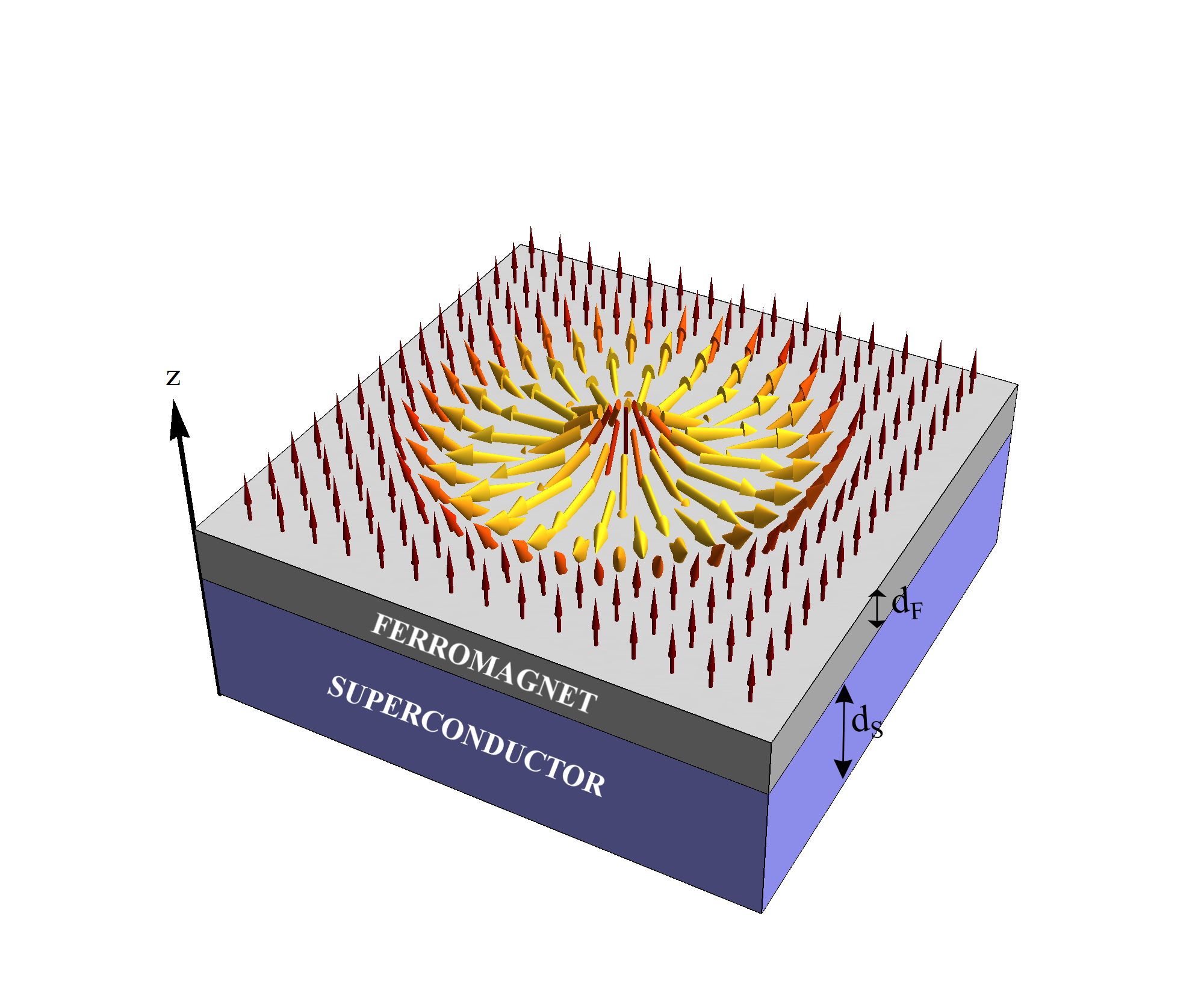
Figure 1: A thin superconducting film proximity-coupled to a ferromagnetic layer hosting a Néel skyrmion. The F layer has thickness $d_{\text{F}}$ and the S layer $d_{\text{S}}$.

Let us consider temperatures for which the superconductivity is well developed, ie. $T\ll T_{c}$ . The free energy of the F/S bilayer can be written as

$$F=F_{0}+F_{\text{sc}}+F_{\text{L}}+F_{\text{mag}}\;,$$ (2)

where $F_{0}$ is the free energy in the absence of superconductivity and magnetic texture, and $F_{\text{sc}}$ is the kinetic term related to the superconducting current energy. To derive the expression of the free energy, we use the London approach which assumes that the generated current does not modify the modulus of the superconducting order parameter. The criterion of applicability of the London approach is well known (see for example Ref. Gennes, 1966): the current density should be much smaller than the critical current density $j_{c}\propto\displaystyle\frac{\Phi_{0}}{\mu_{0}\,\lambda^{2}\,\xi}$, where $\displaystyle\Phi_{0}=\frac{h}{2\,e}$ (with $e>0$) is the superconducting quantum of flux. This is always the case for Abrikosov vortices, except the narrow core region. The computation of the current (see Sec. IV.2) shows that this approach is completely justified to describe the vortex generation by the skyrmion while $R\gg\xi$. Moreover, since we assume that $d_{\text{S}}$ is smaller than $\lambda$, the density of superconducting current energy is nearly constant through the width $d_{\text{S}}$ so $F_{\text{sc}}$ reads:

$$F_{\text{sc}}=\int\frac{1}{2\,\mu_{0}\,\lambda_{\text{eff}}}\left(\vec{\phi}(\vec{r})-\vec{A}(\vec{r})\right)^{2}\mathrm{d}^{2}\vec{r}\,,$$ (3)

where $\displaystyle\lambda_{\text{eff}}=\lambda^{2}/d_{\text{S}}$ is the effective screening length for the superconductor, $\vec{\phi}$ is the gradient of the local superconducting phase (multiplied by $\hbar/2e$), and $\vec{A}$ is the vector potential. Detailed calculations are provided in Appendix A. In the presence of a vortex, the expression for the vector $\vec{\phi}$ can be obtained from the London equation as Gennes (1966):

$$\vec{\phi}(\vec{r})=\frac{\Phi_{0}}{2\,\pi\,r}\vec{e}_{\theta}\,,$$ (4)

where $\vec{e}_{\theta}$ is the unit orthoradial vector.

The third contribution to the free energy, $F_{\text{L}}$ in Eq. (2), corresponds to the coupling energy between the superconductor and the magnetic order induced by the skyrmion. By proximity effect, the interplay between the exchange field and the Rashba spin-orbit interaction in the ferromagnetic layer induces a spin polarization in the superconducting film. This may give rise for example to a spontaneous current in the bulk superconductor near the interface to F, in the absence of an external magnetic field Edelstein (1995); Mironov and Buzdin (2017). For $T$ close to $T_{c}$, such an interaction is described by the Lifshitz invariant Edelstein (1996); Samokhin (2004); Kaur et al. (2005). At low temperatures and for $d_{\text{S}}\ll\lambda$, one can consider that the spin-orbit interaction is averaged over $d_{\text{S}}$. In this case the energy $F_{\text{L}}$ can be written as:

$$F_{\text{L}}=\int\vec{\alpha}(r)\cdot\left(\vec{\phi}(\vec{r})-\vec{A}(\vec{r})\right)\mathrm{d}^{2}\vec{r}\;,$$ (5)

where $\vec{\alpha}(\vec{r})=\alpha(r)\,\vec{e}_{\theta}=-\alpha_{0}\,\sin\Theta(r)\,\vec{e}_{\theta}$ (see Appendix A). The constant $\alpha_{0}$ incorporates the Rashba constant $\alpha_{R}$, the exchange energy $h_{\text{ex}}$, the thickness of the superconducting film $d_{\text{S}}$ and the proximity length $a$:

$$\alpha_{0}\approx\frac{1}{4\,\mu_{0}\,e\,\lambda_{\text{eff}}}\,\frac{a}{d_{\text{S}}}\,\frac{\alpha_{R}\,h_{\text{ex}}}{v_{F}^{2}}\;.$$ (6)

The last component $F_{\text{mag}}$ of the free energy Eq. (2):

$$F_{\text{mag}}=\int\frac{\vec{B}^{2}(\vec{r})}{2\,\mu_{0}}\mathrm{d}^{3}\vec{r}\;,$$ (7)

represents the energy of the magnetic field $\vec{B}=\vec{\nabla}\times\vec{A}$.

The current density for $d_{\text{S}}\ll\lambda$ in the plane $z=0$ is given by $\displaystyle\vec{j}=-\frac{\partial f}{\partial\vec{A}}\,\delta(z)$, where $f$ is the free energy density in the film: $F=\int f\,\mathrm{d}^{2}\vec{r}$. From the Maxwell-Ampere equation $\displaystyle\vec{\nabla}\times\vec{B}=\mu_{0}\,\vec{j}$, we obtain a differential equation for $\vec{A}$, which can be solved in Fourier space Gennes (1966). The solution $\vec{A}_{q}$ of this equation, where $\vec{A}_{q}$ is the two-dimensional Fourier transform of $\vec{A}$ in the layer, is given by:

$$\vec{A}_{q}=\frac{1}{1+2\,q\,\lambda_{\text{eff}}}\,\left(\vec{\phi}_{q}+\mu_{0}\,\lambda_{\text{eff}}\,\vec{\alpha}_{q}\right)\;,$$ (8)

where $\vec{\phi}_{q}$, $\vec{\alpha}_{q}$ are the two-dimensional Fourier transforms of $\vec{\phi}(\vec{r})$ and $\vec{\alpha}(\vec{r})$ respectively. This calculation is provided in Appendix B.1.

III Creation of a superconducting vortex

III.1 Magnetic field induced by the skyrmion

Because of the spontaneous current generated by the skyrmion in the superconducting film, a magnetic field is created perpendicular to the layer. We first consider that there is no vortex. In this case, the term proportional to $\vec{\phi}_{q}$ in Eq.(8) disappears and we can derive the expression of the magnetic field distribution $\vec{B}_{\text{s}}(r)=B_{\text{s}}(r)\,\vec{e}_{z}$ in the superconducting layer. Considering that the skyrmion is small compared to $\lambda_{\text{eff}}$ and focusing on small distances $r$ from the center of the skyrmion ($r\ll\lambda_{\text{eff}}$) one can write;

$$B_{\text{s}}(r)=-\frac{1}{2}\,\mu_{0}\,\alpha_{0}\int q\,\Gamma(q)\,J_{0}(q\,r)\,\mathrm{d}q\;,$$ (9)

where $\Gamma(q)=\displaystyle\int_{0}^{R}r\,\sin(\pi\,\frac{r}{R})\,J_{1}(q\,r)\,\mathrm{d}r$ and $J_{0}(q\,r)$, $J_{1}(q\,r)$ are Bessel functions of first kind. This field distribution is represented by the blue line in Fig. 2. As expected, outside of the skyrmion $B_{\text{S}}$ decreases and vanishes very fast. Moreover, one can check that the magnetic flux associated to $B_{\text{s}}$ equals to zero.

III.2 Vortex nucleation condition

The condition for the superconducting vortex creation can be derived by comparing the free energy of the system with and without a vortex. We replace $\vec{A}$ by its expression, (Eq.8), into the contributions Eq.(3, 5,7) to the free energy . The resulting $F$ can be written as a sum of three terms (see Appendix B.2):

$$F=F_{\text{v}}+F_{\text{s}}+F_{\text{int}}\;.$$ (10)

The first one, proportional to $\Phi_{0}^{2}$, describes the self-energy of the vortex. The second term, proportional to $\alpha_{R}^{2}$, describes the energy of the current induced by the skyrmion, whereas third term, proportional, to $\Phi_{0}\,\alpha_{R}$, the interaction energy between the vortex and such current.

Since $\xi\ll r\ll\lambda_{\text{eff}}$, we can write the self-energy of the vortex in the following way:

$$F_{\text{v}}=\frac{1}{\pi\,\mu_{0}\,\lambda_{\text{eff}}}\left(\frac{\Phi_{0}}{2}\right)^{2}\ln\left(2\,\frac{\lambda_{\text{eff}}}{\xi}\right)\;.$$ (11)

By assuming $R\ll\lambda_{\text{eff}}$, we can write the current energy and the interaction term as

$$F_{\text{s}} = -\frac{\mu_{0}}{8\,\pi}\int\alpha_{q}^{2}\,\mathrm{d}q\;;$$ (12)

$$F_{\text{int}} = -\frac{\Phi_{0}}{2\,\pi\,\mu_{0}\,e\,\lambda_{\text{eff}}}\frac{a}{d_{\text{S}}}\frac{\alpha_{R}\,h_{\text{ex}}}{v_{F}^{2}}\,R\;.$$ (13)

The difference of free energy, $\Delta F=F-F_{\text{s}}$, between the states with and without vortex reads:

$$\Delta F=\frac{\Phi_{0}^{2}}{2\,\pi^{2}\,\mu_{0}\,\lambda_{\text{eff}}}\left[\frac{\pi}{2}\ln\left(2\,\frac{\lambda_{\text{eff}}}{\xi}\right)\right.\\ \left.-\,0.180\,\frac{h_{\text{ex}}}{k_{\text{B}}\,T_{c}}\,\frac{a}{d_{\text{S}}}\,\frac{\alpha_{R}}{v_{\text{F}}}\,\frac{R}{\xi}\right]\;,$$ (14)

where $k_{\text{B}}$ is the Boltzmann constant, $T_{c}$ is the critical temperature of the superconductor and the coherence length is given by $\xi=\displaystyle 0.180\,\frac{\hbar\,v_{F}}{k_{\text{B}}\,T_{c}}$.

The condition for the vortex nucleation is determined by the condition $\Delta F<0$, which gives:

$$\frac{h_{\text{eff}}}{k_{\text{B}}\,T_{c}}\,\frac{\alpha_{R}}{v_{F}}\,\frac{R}{\xi}>\frac{\pi}{0.36}\,\ln\left(2\,\frac{\lambda_{\text{eff}}}{\xi}\right)\;,$$ (15)

where $h_{\text{eff}}=h_{\text{ex}}\,\displaystyle\frac{a}{d_{\text{S}}}$ is the average effective exchange energy, with $a\ll d$.
The condition Eq.(15) gives the features of the ferromagnetic layer required to induce a vortex inside the superconducting film without any external magnetic field. Qualitatively, this result shows that if $\alpha_{R}$, $h_{\text{eff}}$ or $R$ increase, so does the magnetic field $B_{\text{s}}$ (Eq. 9), thereby favoring the appearance of the vortex.

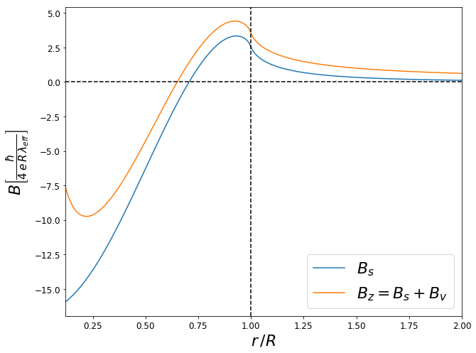
Figure 2: Magnetic field distribution in the superconducting layer. The vortex nucleation condition for a vortex with vorticity 1 is fulfilled: $R=50\,\xi$, $\alpha_{R}=0.1\,v_{F}$ and $h_{\text{eff}}=20\,k_{B}\,T_{c}$. The blue line corresponds to the magnetic field distribution without vortex, whereas the orange one is in the presence of the vortex.

III.3 Multiquanta vortices

We now discuss the possibility of nucleating a vortex carrying $n$ superconducting flux quanta $\Phi_{0}=h/2e$, with $n>1$. So far we only considered the case $n=1$. Let $F_{n}$ be the free energy in presence of a $n$-quanta vortex.

$$F_{n}=n^{2}\,F_{\text{v}}+F_{\text{s}}+n\,F_{\text{int}}\;.$$ (16)

The optimal value of $n$ can be estimated by minimizing $F_{n}$ with respect to $n$:

$$n_{\text{op}}\approx-\frac{F_{\text{int}}}{2\,F_{v}}=\frac{\pi}{0.72\,\ln(2\frac{\lambda_{\text{eff}}}{\xi})}\frac{h_{\text{eff}}}{k_{B}\,T_{c}}\,\frac{\alpha_{R}}{v_{F}}\,\frac{R}{\xi}\;.$$ (17)

Therefore, upon raising the Rashba coupling and/or the exchange field, it is possible to stabilize a multiquanta vortex carrying the integer value of $n_{\text{op}}$ superconducting flux quanta. However for simplicity in what follows we assume that the spin-orbit interaction is weak enough to have a vortex with vorticity larger than 1.

IV Magnetic field and current distributions

IV.1 Magnetic field

The presence of the vortex modifies the magnetic field distribution. In addition to the component $B_{\text{s}}$, stemming from the current induced by the skyrmion in the superconducting layer, there is a term originated from the vortex itself. The total magnetic field distribution can thus be written as

$$B_{z}(r)=B_{\text{s}}(r)+B_{\text{v}}(r)\;.$$ (18)

The term $B_{\text{v}}(r)$ is obtained from the first term of Eq.8:

$$B_{\text{v}}(r)=\frac{\Phi_{0}}{4\,\pi\,\lambda_{\text{eff}}\,r}\;,$$ (19)

for $\xi\ll r\ll\lambda_{\text{eff}}$.
The magnetic field distribution $B_{z}(r)$ is shown in Fig. 2 (orange line). It is assumed that the condition for appearance of a vortex is fulfilled. As expected, both $B_{z}$ and $B_{\text{s}}$ follow the spin direction of the skyrmion, with a sinusoidal-like shape: it is negative near the center, and positive for $r\gtrsim 0.65\,R$. At $r=R$, the amplitude of the magnetic field decreases away from the skyrmion. The component $B_{\text{s}}$ tends to zero very fast, whereas $B_{z}$ vanishes far from the center. It decreases slowly because of the presence of the vortex, whose component $B_{\text{v}}$ is proportional to $1/r$.

IV.2 Charge Current

The current $\vec{J}$ in the superconducting layer is obtained from $\vec{J}=-\displaystyle\frac{\partial f}{\partial\vec{A}}$ (see Appendix C.2). As with the magnetic field distribution, it can be written as the sum of two contributions: one induced directly by the skyrmion, and a second stemming from the vortex.

$$\vec{J}(r)=\vec{J}_{\text{s}}(r)+\vec{J}_{\text{v}}(r)\;.$$ (20)

Under the same assumptions as before, $\xi\ll r\ll\lambda_{\text{eff}}$ and $R\ll\lambda_{\text{eff}}$, one obtains

$$\vec{J}_{\text{s}}(r) = -\alpha_{0}\int q\,\Gamma(q)\,J_{1}(q\,r)\,\mathrm{d}q\,\vec{e}_{\theta}\;;$$ (21)

$$\vec{J}_{\text{v}}(r) = \frac{\Phi_{0}}{2\,\pi\,\mu_{0}\,\lambda_{\text{eff}}\,r}\,\vec{e}_{\theta}\;.$$ (22)

The current lines in the film are shown in Fig. LABEL:fig_courant.a. We use the same parameters as in (Fig. 2).

Around the vortex ($r<0.20\,R$), the current is dominated by the contribution from the vortex and flows anticlockwise. As it can be seen Fig. LABEL:fig_courant.b, in this region the current is positive and decreases like $1/r$. For larger values of $r$ within the skyrmion ($0.20\,R<r<0.95\,R$), the current distribution has a sinusoidal shape, and is dominated by the contribution from the skyrmion. In this region, the current loops are clockwise. Finally, for $r>0.95\,R$, the current is again dominated by the contribution from the vortex. It decreases slowly with distance, and tends to zero far from the skyrmion.

V Conclusion

We have shown that the spontaneous current induced by the skyrmion in the superconducting thin film gives rise to a magnetic field perpendicular to the layer. If the Rashba coupling exceeds a threshold value (given by Eq. 15), the skyrmion can nucleate a superconducting vortex by magnetoelectric proximity effect in the absence of an applied external field. The vorticity is determined by the sign of the spin-orbit interaction and the skyrmion winding. Finally we outline some perspectives implied by our calculations. Even if the Rashba coupling threshold condition is not reached, it is possible to nucleate vortices in S simply by applying an external magnetic field (larger than $H_{c1}$), or in the case when vortices are created directly via the electromagnetic coupling with the ferromagnetic layer. In the former situation (external magnetic field), our free energy calculations demonstrate an attractive coupling which will pin vortices to the skyrmion for one orientation of the magnetic field. For the opposite orientation, the vortices should be pushed away by the skyrmion. Such decoration/antidecoration of the skyrmion by vortices can be, in principle, detected experimentally. Finally, we also stress that the inverse effect, namely the nucleation of a skyrmion via the proximity of a superconducting vortex, is also suggested by our results, a strong effect that could in principle be observed experimentally via magnetic force microscopy or topological Hall effect in systems like Nb/Co/Pt Hrabec et al. (2014).

Appendix A Derivation of the magnetoelectric energy $\mathbf{F_{\text{L}}}$

We derive the expression of the coupling energy between the superconductor and magnetic order induced by the skyrmion. We start from the Ginzburg-Landau free energy

$$F^{\text{GL}}=F^{\text{GL}}_{0}+\int\frac{1}{4\,m}\left|\hat{D}\Psi\right|^{2}\mathrm{d}^{3}\vec{r}+F^{\text{GL}}_{\text{L}}\;,$$ (23)

where $\hat{D}=\left(-\text{i}\,\hbar\,\vec{\nabla}+2\,e\,\vec{A}\right)$ is the gauge-invariant momentum operator and $\Psi=\left|\Psi\right|e^{\text{i}\,\vec{q}\cdot\vec{r}}$. The term $F_{0}^{\text{GL}}$ contains all the terms without derivative of $\Psi$. The Lifshitz invariant $F^{\text{GL}}_{\text{L}}$ reads Edelstein (1996); Samokhin (2004); Kaur et al. (2005):

$$F^{\text{GL}}_{\text{L}}=\int\varepsilon(r)\left(\vec{e}_{z}\times\vec{S}\right)\cdot\left[\Psi^{\star}\,\hat{D}\,\Psi+\text{h.c.}\right]\,\mathrm{d}^{3}\vec{r}\;.$$ (24)

One can derive an estimate of $\varepsilon(r)$, which is constant in the region where the spin-orbit interaction is present and null elsewhere.
To obtain the expression of the wave-vector $\vec{q}$, we must minimize $F^{\text{GL}}$ with respect to $\vec{q}$ for $\vec{A}=\vec{0}$. We get:

$$q=-\frac{4\,m}{\hbar}\varepsilon\;.$$ (25)

From Ref. Dimitrova and Feigel’man, 2007, we have an estimate of $q$:

$$q=\frac{\alpha_{R}\,h_{\text{ex}}}{\hbar\,v_{F}^{2}}\;.$$ (26)

By comparing the expressions 25 and 26, one obtains an estimate of $\varepsilon$:

$$\varepsilon=-\frac{\alpha_{R}\,h_{\text{ex}}}{4\,m\,v_{F}^{2}}\;.$$ (27)

For $T\ll T_{c}$, superconductivity is well developed. We then rewrite the free energy 23 in the London approach by noticing that $\Psi=\left|\Psi\right|e^{\text{i}\,\varphi}$, where $\left|\Psi\right|$ is constant and such that $\left|\Psi\right|^{2}=\frac{1}{2}\,n_{s}$ where $n_{s}$ is the density of superconducting electrons. Thus, the free energy becomes:

$$F=F^{\text{L}}_{0}+\int\frac{e^{2}\,n_{s}}{2\,m}\left(\vec{\phi}-\vec{A}\right)^{2}\mathrm{d}^{3}\vec{r}\\ -e\,n_{s}\,\varepsilon\int\left(\vec{e}_{z}\times\vec{S}\right)\cdot\left(\vec{\phi}-\vec{A}\right)\,\mathrm{d}^{3}\vec{r}\;,$$ (28)

where $\vec{\phi}=-\displaystyle\frac{\Phi_{0}}{2\,\pi}\,\vec{\nabla}\varphi$ and $F^{\text{L}}_{0}=F_{0}+F_{\text{mag}}$. In what follows, $F_{0}$ will be omitted.
We introduce the London coherence length:

$$\lambda^{2}=\frac{m}{\mu_{0}\,n_{s}\,e^{2}}\;.$$ (29)

Considering that $d_{\text{S}}\ll\lambda$, the quantity $\vec{\phi}-\vec{A}$ is almost constant over $d_{\text{S}}$. We emphasize that the spin-orbit interaction and the exchange field penetrate the superconducting layer over a distance $a$, corresponding to the atomic thickness. We also assume that the magnetization in the ferromagnetic layer is weak, thus the Zeeman field is negligible compared to the exchange field. Then we can compute the integrals of Eq. 28 over the z-direction:

$$F=F_{\text{mag}}+\frac{d_{\text{S}}}{2\,\mu_{0}\,\lambda^{2}}\int\left(\vec{\phi}-\vec{A}\right)^{2}\mathrm{d}^{2}\vec{r}\\ -e\,n_{s}\,\varepsilon\,a\int\left(\vec{e}_{z}\times\vec{S}\right)\cdot\left(\vec{\phi}-\vec{A}\right)\,\mathrm{d}^{2}\vec{r}\;.$$ (30)

Introducing the effective screening length $\lambda_{\text{eff}}$, one can notice that the second term of the free energy 30 is exactly the superconducting current energy $F_{\text{sc}}$ (Eq. 3), whereas the third term corresponds to the magnetoelectric energy $F_{\text{L}}$ (Eq. 5).

Appendix B Final expression of the free energy $\mathbf{F}$

B.1 Derivation of the vector potential $\vec{\mathbf{A}}$

In this section, we derive the expression of the vector potential $\vec{A}$. Let $f$ be the free energy density per unit surface.

$$f=\frac{1}{2\,\mu_{0}\,\lambda_{\text{eff}}}\left(\vec{\phi}-\vec{A}\right)^{2}+\vec{\alpha}(r)\cdot\left(\vec{\phi}-\vec{A}\right)+\int\frac{B^{2}}{2\,\mu_{0}}\mathrm{d}z\;.$$ (31)

The current density for $d_{\text{S}}\ll\lambda$ in the plane $z=0$ is given by

$$\vec{j}=-\frac{\partial f}{\partial\vec{A}}\,\delta(z)=\frac{1}{\mu_{0}\,\lambda_{\text{eff}}}\left(\vec{\phi}-\vec{A}\right)\,\delta(z)+\vec{\alpha}(r)\,\delta(z)\;.$$ (32)

We recall the Maxwell-Ampere equation in the London gauge:

$$\mu_{0}\,\vec{j}=\vec{\nabla}\times\vec{B}=-\Delta\vec{A}\;.$$ (33)

By replacing the expression of the current density 32 into the Maxwell-Ampere equation (Eq. 33), one gets:

$$-\Delta\vec{A}+\frac{1}{\lambda_{\text{eff}}}\,\vec{A}\,\delta(z)=\frac{1}{\lambda_{\text{eff}}}\,\vec{\phi}\,\delta(z)+\mu_{0}\,\vec{\alpha}(r)\,\delta(z)\;.$$ (34)

We introduce the following three and two-dimensional Fourier transforms:

$$\vec{A}_{qk} = \int\vec{A}(\vec{r},z)\,e^{\text{i}\left(\vec{q}\cdot\vec{r}+k\,z\right)}\mathrm{d}^{2}\vec{r}\,\mathrm{d}z\;;$$ (35)

$$\vec{A}_{q} = \frac{1}{2\,\pi}\int\vec{A}_{qk}\mathrm{d}k=\int\vec{A}(\vec{r})\,e^{\text{i}\,\vec{q}\cdot\vec{r}}\mathrm{d}^{2}\vec{r}\;;$$ (36)

$$\vec{\phi}_{q} = \int\vec{\phi}(r)\,e^{\text{i}\,\vec{q}\cdot\vec{r}}\mathrm{d}^{2}\vec{r}=\text{i}\,\frac{\Phi_{0}}{q}\,\vec{e}_{\perp}\;;$$ (37)

$$\vec{\alpha}_{q} = \int\vec{\alpha}(r)\,e^{\text{i}\,\vec{q}\cdot\vec{r}}\mathrm{d}^{2}\vec{r}=\text{i}\,\alpha_{q}\,\vec{e}_{\perp}\;,$$ (38)

with $\alpha_{q}=2\,\pi\displaystyle\int_{0}^{\infty}r\,\alpha(r)\,J_{1}(q\,r)\,\mathrm{d}r$ where $J_{1}(q\,r)$ is a Bessel function of first kind. The unit vector $\vec{e}_{\perp}$ is represented in Fig. 4.

Figure 4: The sets of coordinates $\left(\vec{e}_{r},\,\vec{e}_{\theta}\right)$ and $\left(\vec{e}_{q},\,\vec{e}_{\perp}\right)$, respectively corresponding to the real space and the Fourier space.

By taking the Fourier transform of Eq. 34, one obtains the following equation:

$$\vec{A}_{qk}=\frac{1}{q^{2}+k^{2}}\left[\frac{1}{\lambda_{\text{eff}}}\left(\vec{\phi}_{q}-\vec{A}_{q}\right)+\mu_{0}\vec{\alpha}_{q}\right]\;.$$ (39)

After integration of Eq. 39 over $k$, one recovers the expression of $\vec{A}_{q}$ (Eq. 8).

B.2 Free energy $\mathbf{F}$

In this section, we explain how we obtain the expression 10 for the free energy $F$ and how we determine the value of $\eta$ depending on the sign of $\alpha_{\text{R}}$.
Each term of $F$ (Eq. 2) can be written in terms of $\vec{A}_{q}$, $\vec{\phi}_{q}$ and $\vec{\alpha}_{q}$:

$$F_{\text{sc}} = \frac{1}{\left(2\,\pi\right)^{2}}\,\frac{1}{2\,\mu_{0}\,\lambda_{\text{eff}}}\int\left|\vec{\phi}_{q}-\vec{A}_{q}\right|^{2}\,\mathrm{d}^{2}\vec{q}\;;$$ (40)

$$F_{\text{L}} = \frac{1}{\left(2\,\pi\right)^{2}}\int\vec{\alpha}_{q}^{\star}\cdot\left(\vec{\phi}_{q}-\vec{A}_{q}\right)\mathrm{d}^{2}\vec{q}\;;$$ (41)

$$F_{\text{mag}} = \frac{1}{\left(2\,\pi\right)^{3}}\int\frac{\left|\vec{B}_{qk}\right|^{2}}{2\,\mu_{0}}\,\mathrm{d}^{2}\vec{q}\,\mathrm{d}k\;,$$ (42)

where $\vec{B}_{qk}$ is the Fourier transform of $\vec{B}$, and is such that

$$\left|\vec{B}_{qk}\right|^{2}=k^{2}\left|\vec{A}_{qk}\right|^{2}+\left|\left(\vec{q}\times\vec{A}_{qk}\right)\cdot\vec{e}_{z}\right|^{2}\;.$$ (43)

We replace $\vec{A}_{q}$ (Eq. 36) and $\vec{A}_{qk}$ (Eq. 35) by their expression in Eq. 40 to 42. After integration, one obtains:

$$F_{\text{sc}} =\frac{\lambda_{\text{eff}}}{4\,\pi\,\mu_{0}}\int\frac{q}{\left(1+2\,q\,\lambda_{\text{eff}}\right)^{2}}\left(2\,\Phi_{0}-\mu_{0}\,\alpha_{q}\right)^{2}\mathrm{d}q\;;$$ (44)

$$F_{\text{L}} =\frac{1}{2\,\pi}\int\frac{\lambda_{\text{eff}}\,q}{1+2\,q\,\lambda_{\text{eff}}}\left(2\,\Phi_{0}-\mu_{0}\,\alpha_{q}\right)\alpha_{q}\mathrm{d}q\;;$$ (45)

$$F_{\text{mag}} =\frac{1}{2\,\pi\,\mu_{0}}\int\frac{\left(\Phi_{0}+\mu_{0}\,\lambda_{\text{eff}}\,q\,\alpha_{q}\right)^{2}}{\left(1+2\,q\,\lambda_{\text{eff}}\right)^{2}}\mathrm{d}q\;.$$ (46)

Using Eq. 44 to 46, one can rewrite $F$ as a sum of three terms. The first one, proportional to $\Phi_{0}^{2}$, is called $F_{\text{v}}$ (Eq. 11). The second term is proportional to $\alpha_{q}^{2}$, and corresponds to $F_{\text{s}}$ (Eq. 12), and the third one, depending on the product $\Phi_{0}\,\alpha_{q}$, is called $F_{\text{int}}$ (Eq. 13).
In order to nucleate a vortex in the superconducting layer, the difference of energy $\Delta F=F-F_{\text{s}}$ must be negative:

$$\Delta F=\frac{\Phi_{0}^{2}}{2\,\pi^{2}\,\mu_{0}\,\lambda_{\text{eff}}}\left[\frac{\pi}{2}\ln\left(2\,\frac{\lambda_{\text{eff}}}{\xi}\right)\right.\\ \left.+\,0.180\,\eta\,\frac{h_{\text{ex}}}{k_{\text{B}}\,T_{c}}\,\frac{a}{d_{\text{S}}}\,\frac{\alpha_{R}}{v_{\text{F}}}\,\frac{R}{\xi}\right]\;.$$ (47)

The condition $\Delta F<0$ requires that $\eta\,\alpha_{\text{R}}<0$: the polarity of the vortex is determined by the spin-orbit interaction and the skyrmion winding. We thus consider $\alpha_{\text{R}}>0$, which implies $\eta=-1$.

Appendix C Magnetic field and current distributions

C.1 Perpendicular magnetic field distribution $\mathbf{B(r)}$

We compute the normal component $B_{z}(r)$ of the magnetic field distribution, which is given by $B_{z}(r)=\left(\vec{\nabla}\times\vec{A}\right)\cdot\vec{e}_{z}$. In the Fourier space, this relation becomes

$$B^{z}_{qk}=-\text{i}\left(\vec{q}\times\vec{A}_{qk}\right)\cdot\vec{e}_{z}\;,$$ (48)

where $\vec{A}_{qk}$ is obtained from Eq. 39 after replacing $\vec{A}_{q}$ by its expression (Eq. 8). Thus

$$B^{z}_{qk}=\frac{1}{q^{2}+k^{2}}\,\frac{2\,q}{1+2\,q\,\lambda_{\text{eff}}}\left(\Phi_{0}+q\,\lambda_{\text{eff}}\,\mu_{0}\,\alpha_{q}\right)\;.$$ (49)

After integration over $k$, we get the component $B^{z}_{q}$, which is the Fourier transform of $B_{z}(r)$:

$$B^{z}_{q}=\frac{1}{1+2\,q\,\lambda_{\text{eff}}}\left(\Phi_{0}+q\,\lambda_{\text{eff}}\,\mu_{0}\,\alpha_{q}\right)\;.$$ (50)

After taking the inverse Fourier transform of Eq. 50, in the approximation $q\gg\lambda_{\text{eff}}^{-1}$ one obtains the expression 18. Notice that Eq. 19 was previously obtained in Ref. Gennes, 1966.

C.2 Current in the superconducting layer

In this section, we derive the expression of the current $\vec{J}(r)$ in the superconducting layer, obtained from the free energy density (Eq. 31):

$$\vec{J}(r)=-\frac{\partial f}{\partial\vec{A}}=\frac{1}{\mu_{0}\,\lambda_{\text{eff}}}\left(\vec{\phi}-\vec{A}\right)+\vec{\alpha}(r)\;.$$ (51)

In the Fourier space and after replacing $\vec{A}_{q}$ by its expression (Eq. 8), the current becomes:

$$\vec{J}_{q}=\frac{2\,\text{i}}{1+2\,q\,\lambda_{\text{eff}}}\left(\frac{\Phi_{0}}{\mu_{0}}+q\,\lambda_{\text{eff}}\,\alpha_{q}\right)\vec{e}_{\perp}\;.$$ (52)

Taking into account that $\vec{e}_{\perp}=-\sin\theta\,\vec{e}_{r}+\cos\theta\,\vec{e}_{\theta}$ (see Fig. 4), one can perform the inverse Fourier transform of 52. In the approximation $q\gg\lambda_{\text{eff}}^{-1}$, we finally obtain Eq. 20.

References

- Buzdin (2005) A. I. Buzdin, Rev. Mod. Phys. 77, 935 (2005).
- Bergeret et al. (2005) F. S. Bergeret, A. F. Volkov, and K. B. Efetov, Rev. Mod. Phys. 77, 1321 (2005).
- Linder and Robinson (2015) J. Linder and J. W. A. Robinson, Nat. Phys. 11, 307 (2015).
- Blamire and Robinson (2014) M. G. Blamire and J. W. A. Robinson, J. Phys. Condens. Matter 26, 453201 (2014).
- Kitaev (2001) A. Y. Kitaev, Physics-Uspekhi 44, 131 (2001).
- Nayak et al. (2008) C. Nayak, S. H. Simon, A. Stern, M. Freedman, and S. Das Sarma, Reviews of Modern Physics 80, 1083 (2008).
- Oreg et al. (2010) Y. Oreg, G. Refael, and F. von Oppen, Phys. Rev. Lett. 105, 177002 (2010).
- Lutchyn et al. (2010) R. M. Lutchyn, J. D. Sau, and S. Das Sarma, Phys. Rev. Lett. 105, 077001 (2010).
- Wu et al. (2017) C.-T. Wu, B. M. Anderson, W.-H. Hsiao, and K. Levin, Phys. Rev. B 95, 014519 (2017).
- Black-Schaffer and Linder (2011) A. M. Black-Schaffer and J. Linder, Phys. Rev. B 84, 180509 (2011).
- Alicea (2012) J. Alicea, Rep. Prog. Phys. 75, 076501 (2012).
- Buzdin (2008) A. Buzdin, Phys. Rev. Lett. 101, 107005 (2008).
- Konschelle and Buzdin (2009) F. Konschelle and A. Buzdin, Phys. Rev. Lett. 102, 017001 (2009).
- Ojanen (2012) T. Ojanen, Phys. Rev. Lett. 109, 226804 (2012).
- Pershoguba et al. (2015) S. S. Pershoguba, K. Björnson, A. M. Black-Schaffer, and A. V. Balatsky, Phys. Rev. Lett. 115, 116602 (2015).
- Chudnovsky (2017) E. M. Chudnovsky, Phys. Rev. B 95, 100503 (2017).
- Konschelle et al. (2015) F. Konschelle, I. V. Tokatly, and F. S. Bergeret, Phys. Rev. B 92, 125443 (2015).
- Bergeret and Tokatly (2015) F. S. Bergeret and I. V. Tokatly, EPL 110, 57005 (2015).
- Fominov et al. (2007) Y. V. Fominov, A. F. Volkov, and K. B. Efetov, Phys. Rev. B 75, 104509 (2007).
- Kulagina and Linder (2014) I. Kulagina and J. Linder, Phys. Rev. B 90, 054504 (2014).
- Konschelle et al. (2016) F. Konschelle, I. V. Tokatly, and F. S. Bergeret, Phys. Rev. B 94, 014515 (2016).
- Halterman et al. (2008) K. Halterman, O. T. Valls, and P. H. Barsic, Phys. Rev. B 77, 174511 (2008).
- Braude and Nazarov (2007) V. Braude and Y. V. Nazarov, Phys. Rev. Lett. 98, 077003 (2007).
- Mironov and Buzdin (2017) S. Mironov and A. Buzdin, Phys. Rev. Lett. 118, 077001 (2017).
- Silaev et al. (2017) M. A. Silaev, I. V. Tokatly, and F. S. Bergeret, Phys. Rev. B 95, 184508 (2017).
- Robinson et al. (2010) J. W. A. Robinson, J. D. S. Witt, and M. G. Blamire, Science 329, 59 (2010).
- Bergeret and Tokatly (2014) F. S. Bergeret and I. V. Tokatly, Phys. Rev. B 89, 134517 (2014).
- Mel’nikov et al. (2012) A. S. Mel’nikov, A. V. Samokhvalov, S. M. Kuznetsova, and A. I. Buzdin, Phys. Rev. Lett. 109, 237006 (2012).
- Bogdanov and Yablonskii (1989) A. N. Bogdanov and D. A. Yablonskii, Sov. Phys. JETP 68, 101 (1989).
- Rößler et al. (2011) U. K. Rößler, A. A. Leonov, and A. N. Bogdanov, Journal of Physics: Conference Series 303, 012105 (2011).
- Leonov et al. (2016) A. O. Leonov, T. L. Monchesky, N. Romming, A. Kubetzka, A. N. Bogdanov, and R. Wiesendanger, New J. Phys. 18, 065003 (2016).
- Jonietz et al. (2010) F. Jonietz, S. Mühlbauer, C. Pfleiderer, A. Neubauer, W. Münzer, A. Bauer, T. Adams, R. Georgii, P. Böni, R. A. Duine, K. Everschor, M. Garst, and A. Rosch, Science 330 (2010).
- Yu et al. (2012) X. Yu, N. Kanazawa, W. Zhang, T. Nagai, T. Hara, K. Kimoto, Y. Matsui, Y. Onose, and Y. Tokura, Nat. Commun. 3 (2012).
- Kiselev et al. (2011) N. S. Kiselev, A. N. Bogdanov, R. Schäfer, and U. K. Rößler, J. Phys. D: Appl. Phys. 44 (2011).
- Iwasaki et al. (2013) J. Iwasaki, M. Mochizuki, and N. Nagaosa, Nature Nanotech. 8, 742 (2013).
- Hrabec et al. (2017) A. Hrabec, J. Sampaio, M. Belmeguenai, I. Gross, R. Weil, S. M. Chérif, A. Stashkevich, V. Jacques, A. Thiaville, and S. Rohart, Nat. Commun. 8, 15765 (2017).
- Fraerman et al. (2005) A. A. Fraerman, I. R. Karetnikova, I. M. Nefedov, I. A. Shereshevskii, and M. A. Silaev, Phys. Rev. B 71, 094416 (2005).
- Vadimov et al. (2018) V. L. Vadimov, M. V. Sapozhnikov, and A. S. Mel’nikov, Appl. Phys. Lett. 113, 032402 (2018).
- Rabinovich et al. (2018) D. S. Rabinovich, I. V. Bobkova, A. M. Bobkov, and M. A. Silaev, Phys. Rev. B 98, 184511 (2018).
- Yang et al. (2016) G. Yang, P. Stano, J. Klinovaja, and D. Loss, Phys. Rev. B 93, 224505 (2016).
- Güngördü et al. (2018) U. Güngördü, S. Sandhoefner, and A. A. Kovalev, Phys. Rev. B 97, 115136 (2018).
- Takashima and Fujimoto (2016) R. Takashima and S. Fujimoto, Phys. Rev. B 94, 235117 (2016).
- Pershoguba et al. (2016) S. S. Pershoguba, S. Nakosai, and A. V. Balatsky, Phys. Rev. B 94, 064513 (2016).
- Hals et al. (2016) K. M. Hals, M. Schecter, and M. S. Rudner, Phys. Rev. Lett. 117, 017001 (2016).
- Nagaosa and Tokura (2013) N. Nagaosa and Y. Tokura, Nature Nanotech. 8, 899 (2013).
- Lyuksyutov and Pokrovsky (2005) I. F. Lyuksyutov and V. L. Pokrovsky, Adv. Phys. 54, 67 (2005).
- Gennes (1966) P. G. D. Gennes, Superconductivity of Metals and Alloys (Benjamin, 1966).
- Edelstein (1995) V. M. Edelstein, Phys. Rev. Lett. 75, 2004 (1995).
- Edelstein (1996) V. M. Edelstein, J. Phys. Condens. Matter 8, 339 (1996).
- Samokhin (2004) K. V. Samokhin, Phys. Rev. B 70, 104521 (2004).
- Kaur et al. (2005) R. P. Kaur, D. F. Agterberg, and M. Sigrist, Phys. Rev. Lett. 94, 137002 (2005).
- Hrabec et al. (2014) A. Hrabec, N. A. Porter, A. Wells, M. J. Benitez, G. Burnell, S. McVitie, D. McGrouther, T. A. Moore, and C. H. Marrows, Phys. Rev. B 90, 020402 (2014).
- Dimitrova and Feigel’man (2007) O. Dimitrova and M. V. Feigel’man, Phys. Rev. B 76, 014522 (2007).