Subtleties in the interpretation of hazard ratios

Summary

The hazard ratio is one of the most commonly reported measures of treatment effect in randomised trials, yet the source of much misinterpretation. This point was made clear by Hernán, (2010) in commentary, which emphasised that the hazard ratio contrasts populations of treated and untreated individuals who survived a given period of time, populations that will typically fail to be comparable - even in a randomised trial - as a result of different pressures or intensities acting on both populations. The commentary has been very influential, but also a source of surprise and confusion. In this note, we aim to provide more insight into the subtle interpretation of hazard ratios and differences, by investigating in particular what can be learned about treatment effect from the hazard ratio becoming 1 after a certain period of time. Throughout, we will focus on the analysis of randomised experiments, but our results have immediate implications for the interpretation of hazard ratios in observational studies.

Keywords: Causality; Cox regression; Hazard ratio; Randomized study; Survival analysis.

1 Introduction

The popularity of the Cox regression model has contributed to the enormous success of the hazard ratio as a concise summary of the effect of a randomised treatment on a survival endpoint. Notwithstanding this, use of the hazard ratio has been criticised over recent years. Hernán, (2010) argued that selection effects render a causal interpretation of the hazard ratio difficult when treatment affects outcome. While the treated and untreated people are comparable by design at baseline, the treated people who survive a given time $t$ may then tend to be more frail (as a result of lower mortality if treatment is beneficial) than the untreated people who survive the given time $t$, so that the crucial comparability of both groups is lost at that time. Aalen et al., (2015) re-iterated Hernán’s concern. They viewed the problem more as one of non-collapsibility (Martinussen and Vansteelandt,, 2013), which is a concern about the interpretation of the hazard ratio, though not about its justification as a causal contrast. In particular, they argued that the magnitude of the hazard ratio typically changes as one evaluates it in smaller subgroups of the population (e.g. frail people), even in the absence of interaction effects on the log hazard scale. In this paper, we aim to develop more insight into these matters. We will focus in particular on what can be learned about the treatment effect from the hazard ratio becoming 1 after a certain point in time. Throughout, we will assume that data are available from a randomised experiment on the effect of a dichotomous treatment $A$ (coded 1 for treatment and 0 for control) on a survival endpoint $T$, so that issues of confounding can be ignored, although our findings naturally extend to observational studies.

2 The Cox model and causal reasoning

Analyses of time-to-event endpoints in randomised experiments are commonly based on the Cox model

$$\lambda(t;a)=\lambda_{0}(t)e^{\beta a},$$

where $\lambda(t;a)$ denotes the hazard function of $T$ given $A=a$, evaluated at time $t$, and $\lambda_{0}(t)$ is the unspecified baseline hazard function. This model implies that for all $t$

$$P(T>t|A=1)=P(T>t|A=0)^{\exp(\beta)},$$ (1)

which suggests that the exponential of $\beta$ can be interpreted as

$$\exp(\beta)=\frac{\log P(T>t|A=1)}{\log P(T>t|A=0)}.$$

This represents a causal contrast (i.e., it compares the same population under different interventions). Indeed, let $T^{a}$ denote the potential event time we would see if the exposure $A$ is set to $a$. Then, since randomisation ensures that $T^{a}\perp\!\!\!\perp A$ for $a=0,1$, we have that

$$\exp(\beta)=\frac{\log P(T^{1}>t)}{\log P(T^{0}>t)}.$$

This shows that, under the proportional hazard assumption, $\exp(\beta)$ forms a relative contrast of what the log survival probability would be at an arbitrary time $t$ if everyone were treated, versus what it would be at that time if no one were treated.

The log-transformation makes the above interpretation of $\exp(\beta)$, while causal, difficult. It is therefore more common to interpret $\exp(\beta)$ as a hazard ratio

$$\exp(\beta)=\frac{\lim_{h\rightarrow 0}P(t\leq T<t+h|T\geq t,A=1)}{\lim_{h\rightarrow 0}P(t\leq T<t+h|T\geq t,A=0)}=\frac{\lim_{h\rightarrow 0}P(t\leq T^{1}<t+h|T^{1}\geq t)}{\lim_{h\rightarrow 0}P(t\leq T^{0}<t+h|T^{0}\geq t)}.$$

Interpretation appears simpler now, but this is somewhat deceptive for two reasons. First, the righthand expression shows that $\exp(\beta)$ contrasts the hazard functions with and without intervention for two separate groups of individuals, those who survive time $t>0$ with treatment ($T^{1}\geq t$) and those who survive time $t>0$ without treatment ($T^{0}\geq t$). Those groups will typically fail to be comparable if treatment affects outcome (Hernán,, 2010). In particular, when treatment has a beneficial effect then, despite randomisation, the subgroup $T^{1}\geq t$ in the numerator will generally contain more frail people than the subgroup $T^{0}\geq t$ in the denominator, where the frailest people may have died already. When viewed as a hazard ratio, $\exp(\beta)$ therefore does not represent a causal contrast. Second, the interpretation of $\exp(\beta)$ as a hazard ratio is further complicated by it being non-collapsible, so that its magnitude typically becomes more pronounced as one evaluates smaller subgroups of the study population (Martinussen and Vansteelandt,, 2013; Aalen et al.,, 2015).

The summary so far is that, under the assumption of proportional hazards, the parameter $\exp(\beta)$ in the Cox model expresses a causal effect, namely the ratio of log survival probabilities with versus without treatment in the study population. Because this interpretation is not insightful, results are best communicated by visualising identity (1) in terms of estimated survival curves with versus without treatment (Hernán,, 2010). This has the advantage that it provides better insight into the possible public health impact of the intervention, but the drawback that it does not permit a compact way of reporting and that survival curves do not provide an understanding of a possible dynamic treatment effect. To enable a more in-depth understanding, it is tempting to interpret $\exp(\beta)$ as a hazard ratio, but then interpretation becomes subtle. We will demonstrate this in more detail in the next section, where we will investigate to what extent hazard ratios may provide insight into the dynamic nature of the treatment effect.

3 Time-varying hazard ratios are not causally interpretable

Consider now a study where the hazard ratio changes with time in the following sense:

$$\frac{\lambda(t;A=1)}{\lambda(t;A=0)}=\left\{\begin{array}[]{ll}\exp(\beta_{1})&\textrm{if $t\leq\nu$}\\ \exp(\beta_{2})&\textrm{if $t>\nu$}\\ \end{array}\right.$$ (2)

with $\beta_{1}\neq\beta_{2}$, where $\nu>0$ denotes the change point, which we assume to be known based on subject matter knowledge. Suppose in particular that $\beta_{1}<0$ and $\beta_{2}=0$. This is commonly interpreted as if treatment is initially beneficial, but becomes ineffective from time $\nu$ onwards. We present a practical example in Section 4.2 where this situation arises. In the following sections, we will reason whether such interpretation is justified, and thus whether hazard ratios permit a dynamic understanding of the treatment effect.

3.1 A closer look at the causal mechanism

To develop a greater understanding, we will first develop insight into data-generating processes (DGP) that could give rise to (2). Let $Z$ represent the participants’ unmeasured baseline frailty (higher means more frail), which affects $T$, but is independent of $A$ by randomisation. Suppose that the hazard function $\lambda(t;a,z)$ of $T$ given $A=a$ and $Z=z$ satisfies

$$\lambda(t;a,z)=z\lambda^{*}(t;a),$$ (3)

for some function $\lambda^{*}(t;a)$, and let $Z$ be Gamma distributed with mean 1 and variance $\theta$. This specific choice is not essential, however, and we later consider a situation where $Z$ is binary.

We will investigate what choices of $\lambda^{*}(t;a)$ give rise to model (2). With $\phi_{Z}(u)=E(e^{-Zu})$ the Laplace transform associated with the distribution of $Z$, the following relationship between the hazard function of interest $\lambda(t;A)$, and $\lambda^{*}(t;A)$, can be shown to hold:

$$\Lambda^{*}(t;a)=\phi_{Z}^{-1}(e^{-\Lambda(t;a)})=\frac{1-e^{-\theta\Lambda(t;a)}}{\theta e^{-\theta\Lambda(t;a)}},$$

where $\Lambda(t;a)=\int_{0}^{t}\lambda(s;a)\,ds$ and similarly with $\Lambda^{*}(t;a)$. Simple calculations then show that model (3) implies model (2) when

$$\lambda(t;A,Z)=\left\{\begin{array}[]{ll}Z\lambda_{0}(t)e^{\beta_{1}A}\exp{\{\theta\Lambda_{0}(t)e^{\beta_{1}A}\}}&\textrm{if $t\leq\nu$}\\ Z\lambda_{0}(t)e^{\beta_{2}A}\exp{\left\{\theta\Lambda_{0}(\nu)e^{\beta_{1}A}+\theta\Lambda_{0}(\nu,t)e^{\beta_{2}A}\right\}}&\textrm{if $t>\nu$}\\ \end{array}\right.$$ (4)

where $\Lambda_{0}(\nu,t)=\int_{\nu}^{t}\lambda_{0}(s)\,ds$. For subjects with given $Z=z$, it follows that the conditional hazard ratio, which we term $\mbox{HR}_{Z}(t)$, is

$$\frac{\lambda(t;A=1,Z)}{\lambda(t;A=0,Z)}=\left\{\begin{array}[]{ll}\exp(\beta_{1})\exp{[\theta\Lambda_{0}(t)\{\exp(\beta_{1})-1\}]}&\textrm{if $t\leq\nu$}\\ \exp(\beta_{2})\exp{[\theta\Lambda_{0}(\nu)\{\exp(\beta_{1})-1\}+\theta\Lambda_{0}(\nu,t)\{\exp(\beta_{2})-1\}]}&\textrm{if $t>\nu$}\\ \end{array}\right.$$

For $\beta_{2}=0$, this simplifies to

$$\frac{\lambda(t;A=1,Z)}{\lambda(t;A=0,Z)}=\left\{\begin{array}[]{ll}\exp(\beta_{1})\exp{[\theta\Lambda_{0}(t)\{\exp(\beta_{1})-1\}]}&\textrm{if $t\leq\nu$}\\ \exp{[\theta\Lambda_{0}(\nu)\{\exp(\beta_{1})-1\}]}&\textrm{if $t>\nu$}\\ \end{array}\right.$$

which is smaller than 1 at all time points when, as previously assumed, $\beta_{1}<0$. We conclude that treatment appears beneficial at all times amongst individuals with the same value $z$ of $Z$, regardless of $z$. This contradicts the earlier, naïve interpretation that, across all individuals combined, treatment is ineffective from time $\nu$ onwards.

The root cause of these contradictory conclusions is the fact that the hazard ratio at a given time does not express a causal effect (Hernán,, 2010). This has nothing to do with model misspecification, as all considered models hold by construction. In particular, when $\beta_{2}=0$ and $\theta=1$, then

$$\frac{E(Z|T>t,A=1)}{E(Z|T>t,A=0)}=\left\{\begin{array}[]{ll}\exp{\{\Lambda_{0}(t)(1-e^{\beta_{1}})\}}&\textrm{if $t\leq\nu$}\\ \frac{\exp{\{\Lambda_{0}(\nu)\}}+\Lambda_{0}(\nu,t)}{\exp{\{\Lambda_{0}(\nu)e^{\beta_{1}}\}}+\Lambda_{0}(\nu,t)}&\textrm{if $t>\nu$}.\end{array}\right.$$

While $Z$ is independent of $A$ by randomisation, it is thus no longer so amongst subgroups of survivors, where we are left with more frail subjects in the active treatment group: $E(Z|T>t,A=1)>E(Z|T>t,A=0)$. That selection takes place does not rely on $Z$ being Gamma-distributed; see Appendix A.1, where we consider a situation with a binary frailty variable.

To illustrate further, we generated a single data set with $Z$ binary with $P(Z=0.2)=0.2$ and $P(Z=1.2)=0.8$ corresponding to low and high risk groups. The treatment variable $A$ was binary with $P(A=1|Z)=0.5$. Further, we took $\beta_{1}=-\log{(2)}$, $\beta_{2}=0$, the baseline hazard function $\lambda_{0}(t)=0.4$, and the change point $\nu=4$. We took a large sample size $n=20000$ so that sampling variability is small, and induced censoring according to a uniform distribution on $[0,10]$, randomly for half of the individuals, and the rest censored at $t=8$, resulting in an overall censoring percent of approximately 19%. The result from a change point Cox analysis was $\hat{\beta}_{1}=-0.67$ (SE 0.018) and $\hat{\beta}_{2}=-0.03$ (SE 0.034). The corresponding hazard ratios are $0.51$ for $t\leq 4$ and $1.03$ for $t>4$. In contrast, the conditional hazard ratio in Figure 1 is seen to be smaller than 1 at all times, not only in the first initial period. Indeed, no matter the value of $Z$, it lies between 0.33 and 0.80 in the considered time period from 0 to 8.

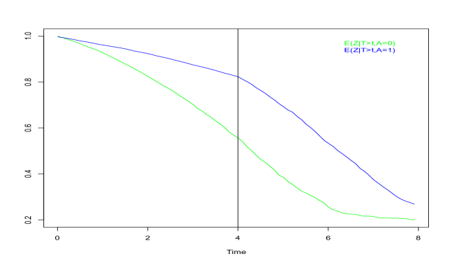
Figure 2: Simulation study. Plot of $E(Z|T>t,A=a)$, $a=0,1$.

That we are misled by the hazard ratios calculated from the extended Cox regression analysis is due to selection taking place. This is shown in Figure 2, where we have plotted $E(Z|T>t,A=a)$ for $a=0,1$. Since the treatment has a beneficial effect, we are left with more and more frail subjects in this group compared to the untreated group. In Figure 2, the blue curve ($A=1$) therefore lies consistently above the green curve ($A=0$).

As just shown, the DGP given by $\lambda(t;A,Z)$ with $\nu=\infty$ implies the marginal Cox model. It is tempting to interpret $\mbox{HR}_{Z}(t)$ as a causal hazard ratio, but this only holds under further untestable assumptions as shown in Section 3.2 and 3.4. In Appendix A.2, we formulate a more general DGP so that both the marginal Cox model and the model $\lambda(t;A,Z)$ are correctly specified.

3.2 Towards a causal hazard ratio

To remedy this problem, it seems intuitively of interest to evaluate conditional hazard ratios

$$\frac{\lim_{h\rightarrow 0}P(t\leq T<t+h|T\geq t,A=1,Z=z)}{\lim_{h\rightarrow 0}P(t\leq T<t+h|T\geq t,A=0,Z=z)}=\frac{\lim_{h\rightarrow 0}P(t\leq T^{1}<t+h|T^{1}\geq t,Z=z)}{\lim_{h\rightarrow 0}P(t\leq T^{0}<t+h|T^{0}\geq t,Z=z)},$$

for a large collection of baseline variables $Z$, such that those who survive time $t>0$ with treatment ($T^{1}\geq t$) are comparable to those who survive time $t>0$ without treatment ($T^{0}\geq t$), but have the same covariate values $z$. Such comparability would be attained if

$$T^{1}\perp\!\!\!\perp T^{0}|Z.$$ (5)

Under this assumption, it follows via Bayes’ rule that the righthand side of the above identity equals

$$\frac{\lim_{h\rightarrow 0}P(t\leq T^{1}<t+h|T^{0}\geq t,T^{1}\geq t,Z=z)}{\lim_{h\rightarrow 0}P(t\leq T^{0}<t+h|T^{0}\geq t,T^{1}\geq t,Z=z)}.$$ (6)

This estimand expresses the instantaneous risk at time $t$ on treatment versus control for the principal stratum of individuals with covariates $z$ who would have survived up to time $t$, no matter what treatment. It represents a causal contrast, which is closely related to the so-called survivor average causal effect (Rubin,, 2000). We will refer to it as the conditional causal hazard ratio.

Unfortunately, the assumption (5) is untestable and biologically implausible, as it is essentially impossible to believe that one can get hold of all predictors of the event time such that knowledge of the event time without treatment does not further predict the event time with treatment. Furthermore, even if one could get hold of all such predictors, then because $Z$ would probably carry so much information about the event time, one would logically expect the numerator and denominator of (6) to be so close to 0 or 1 that it would render the conditional causal hazard ratio essentially meaningless. Below, we will therefore focus on the marginal causal hazard ratio $\mathrm{HR}(t)$ obtained from (6) with $Z$ empty:

$$\mathrm{HR}(t)=\frac{\lim_{h\rightarrow 0}P(t\leq T^{1}<t+h|T^{0}\geq t,T^{1}\geq t)}{\lim_{h\rightarrow 0}P(t\leq T^{0}<t+h|T^{0}\geq t,T^{1}\geq t)}.$$ (7)

3.3 Why causal hazard ratios are not identified without strong assumptions

The reason why the causal hazard ratio (7) is not identifiable without invoking strong assumptions is that it attempts to answer an overly ambitious question. Imagine a trial that randomises participants over an implanted medical device (e.g. a stent or a pacemaker) versus no treatment (or placebo). Suppose that the medical device gradually deteriorates and stops being operational after some time $\nu$. Then we would say that treatment no longer works from time $\nu$ onwards. This would correspond with $\mathrm{HR}(t)=1$ for $t\geq\nu$. However, how could data from a randomised trial be informative about the effect of treatment after time $\nu$ when no information is collected on the times at which the medical device is operational or not? To learn about the treatment effect at each time $t$, we should ideally need data $A_{t}$ on whether ($A_{t}=1$) or not ($A_{t}=0)$ the device is operational at that time. When the operation time is ignorable, then one may learn about the treatment effect at each time $t$ through contrasts of the form

$$\frac{\lim_{h\rightarrow 0}P(s\leq T<s+h|T\geq s,\overline{A}_{t-}=1,A_{t}=1)}{\lim_{h\rightarrow 0}P(s\leq T<s+h|T\geq s,\overline{A}_{t-}=1,A_{t}=0)},$$

for all $s\geq t$, where $\overline{A}_{t-}$ is the information generated by all $A_{u}$, $u<t$. It is unsurprising that without detailed data on the operation times of each device, strong assumptions are needed to develop insight into the dynamic nature of the treatment effect. Likewise, consider a trial that randomises participants over a once-daily treatment regimen versus placebo. Then we would say that treatment no longer works from time $\nu$ onwards when, from that time onwards, patients with the same history of treatment experience the same outcomes (in distribution), whether or not they continue treatment. To infer when treatment becomes ineffective, a multi-stage design is ideally needed where patients on the treatment arm may randomly be switched to the control arm at designated points in time. Without such design, some progress can still be made with data on daily pill intake. However, without such design and data, inferring when treatment becomes ineffective remains an ambitious undertaking.

3.4 Sensitivity analysis

Some further insight into the magnitude of the causal hazard ratio at a given time $t$ can be obtained under the monotonicity assumption that no one is harmed by treatment, i.e.

$$T^{1}\geq T^{0}\quad\mathrm{with\ probability\ 1}.$$

Under this assumption, we can write

$$P(t\leq T<t+h|T\geq t,A=0)=P(t\leq T^{0}<t+h|T^{0}\geq t)=P(t\leq T^{0}<t+h|T^{0}\geq t,T^{1}\geq t)$$

and

$$P(t\leq T<t+h|T\geq t,A=1) = P(t\leq T^{1}<t+h|T^{1}\geq t)$$

$$= P(t\leq T^{1}<t+h|T^{0}\geq t,T^{1}\geq t)\pi(t)$$

$$+P(t\leq T^{1}<t+h|T^{0}<t,T^{1}\geq t)\left\{1-\pi(t)\right\},$$

with

$$\pi(t) \equiv P(T^{0}\geq t|T^{1}\geq t)=\frac{P(T^{0}\geq t)}{P(T^{1}\geq t)}=\frac{P(T\geq t|A=0)}{P(T\geq t|A=1)}.$$

It follows that

$$\frac{\lambda(t;A=1)}{\lambda(t;A=0)}=\mathrm{HR}(t)\left[\pi(t)+\mathrm{SR}(t)\left\{1-\pi(t)\right\}\right],$$ (8)

where

$$\mathrm{SR}(t)\equiv\frac{\lim_{h\rightarrow 0}P(t\leq T^{1}<t+h|T^{0}<t,T^{1}\geq t)}{\lim_{h\rightarrow 0}P(t\leq T^{1}<t+h|T^{0}\geq t,T^{1}\geq t)}.$$

compares the instantaneous risk at time $t$ on treatment for individuals who remained event-free at time $t$ thanks to treatment versus individuals who would have been event-free at time $t$ regardless of treatment. It can be viewed as a selection effect and is therefore termed a sensitivity ratio (SR). Expression (8) thus conveys that the dependence of the hazard ratio ${\lambda(t;A=1)}/{\lambda(t;A=0)}$ on time $t$ may differ from the causal hazard ratio on time as a result of selection effects. In particular, when the observed hazard ratio ${\lambda(t;A=1)}/{\lambda(t;A=0)}$ is constant, e.g. suggesting a beneficial treatment effect of 0.8, then this will often correspond with a more pronounced treatment effect $\mbox{HR}(t)\leq 0.8$. This results from (8), if $\mbox{SR}(t)\geq 1$, as $0\leq\pi(t)\leq 1$. The causal hazard ratio $\mbox{HR}(t)$ then need not be constant. This may be the result of varying treatment effectiveness over time, but may also be the result of the patient population (the principal stratum $T^{0}\geq t,T^{1}\geq t$) changing with time. It follows from the above results that

$$\mathrm{HR}(t)=\frac{\lambda(t;A=1)}{\lambda(t;A=0)}\left[\pi(t)+\mathrm{SR}(t)\left\{1-\pi(t)\right\}\right]^{-1}.$$

All terms in the righthand side, apart from $\mbox{SR}(t)$, are identified from the observed data. The above expression may therefore be used as the basis of a sensitivity analysis where the user tries different choices of $\mbox{SR}(t)$. However, it is not clear what would be reasonable values of $\mbox{SR}(t)$, and the monotonicity assumption may also not be plausible.

Assume instead that there is a $Z$ so that (5) holds, and so that the DGP is governed by

$$\lambda(t;A,Z)=\exp{\{\psi_{0}(t,A)+\psi_{1}(t,Z)\}}$$ (9)

for some general functions $\psi_{0}$ and $\psi_{1}$, then

$$\mbox{HR}(t)=\frac{E\{P(T^{1}=t|T^{1}\geq t,Z)|T^{0}\geq t,T^{1}\geq t\}}{E\{P(T^{0}=t|T^{0}\geq t,Z)|T^{0}\geq t,T^{1}\geq t\}}=\exp{\{{\psi_{0}(t,1)-\psi_{0}(t,0)\}}=\mbox{HR}_{Z}(t)}$$

Thus, if (5) and (9) hold then $\mbox{HR}(t)=\mbox{HR}_{Z}(t)$. In the worked application in Section 4.1 we compare $\mbox{HR}(t)$ to the Cox hazard ratio while modelling the correlation between $T^{0}$ and $T^{1}$ letting $Z$ be Gamma distributed with varying variance so that (5) and (9) hold. As a further illustration we now describe how to simulate data so that (5) and (9) are fulfilled, and so that the marginal Cox model, conditioning only on $A$, is also correctly specified. Take $A$, $Z$, $V_{0}$ and $V_{1}$ to be independent so that $Z$ is Gamma distributed with mean 1 and variance $\theta$, $V_{0}$ and $V_{1}$ are exponentially distributed with mean 1, and the exposure $A$ is binary with $P(A=1)=1/2$. Then let $T^{0}=\frac{1}{\theta}\log{(\frac{\theta}{Z}V_{0}+1)},$ $T^{1}=\frac{1}{\theta e^{\beta}}\log{(\frac{\theta}{Z}V_{1}+1)},$ and let $T=(1-A)T^{0}+AT^{1}.$ It follows directly that (5) holds, and further that the marginal Cox model is correctly specified, and also that

$$\lambda(t;A,Z)=Z\exp{\{\beta A+\theta e^{\beta A}t\}}$$

so (9) also holds. Thus, $\mbox{HR}(t)=\mbox{HR}_{Z}(t)$, and

$$\mbox{HR}(t)=e^{\beta}\exp{\{t\theta(e^{\beta}-1)\}}.$$

Different values of $\theta$ will give different values of Kendall’s $\tau$ corresponding to different correlation between $T^{0}$ and $T^{1}$. In the specific setting, we have $\tau=\theta/(\theta+2)$. Figure 3 displays $\mbox{HR}(t)$ in scenarios with different values of Kendall’s $\tau$. Note that the marginal Cox model induces the hazard ratio $e^{\beta}$, which is taken to be $e^{\beta}=0.5$. It is seen that $\mbox{HR}(t)$ is equal to $e^{\beta}$ only under independence between $T^{0}$ and $T^{1}$; otherwise $\mbox{HR}(t)$ looks like a decreasing function in $t$ with $\mbox{HR}(0)=e^{\beta}$. When $T^{0}$ and $T^{1}$ are highly correlated (Kendall’s $\tau=0.93$) then $\mbox{HR}(t)$ is sharply decreasing towards zero. In Appendix A.4 we describe another DGP where again (5) holds and the marginal Cox model is correctly specified, but $\mbox{HR}(t)$ and $\mbox{HR}_{Z}(t)$ are different due to failure of (9).

3.5 Hazard differences

Under some conditions, hazard differences - as opposed to hazard ratios - have a more appealing interpretation, apart from them being collapsible (Martinussen and Vansteelandt,, 2013). In particular, suppose that the additive hazards model

$$\lambda(t;A,Z)=\psi(t)A+\omega(t,Z),$$ (10)

holds for general functions $\psi$, $\omega$ and baseline covariates $Z$. It has been shown that under this model, the baseline exchangeability of treated and untreated individuals w.r.t. the covariates $Z$, as guaranteed by randomisation, implies that $A\perp\!\!\!\perp Z|T>t$ (Vansteelandt et al.,, 2014; Aalen et al.,, 2015). However, since this is equivalent to

$$P(Z=z\,|\,T^{0}>t)=P(Z=z\,|\,T^{1}>t),$$ (11)

it does not mean that there is a balance in the risk set, because (11) shows that this is a comparison between two different groups of people: those with $T^{0}>t$ and those with $T^{1}>t$. Indeed, the hazard difference

$$\psi(t)=\lim_{h\rightarrow 0}P(t\leq T^{1}<t+h|T^{1}\geq t)-\lim_{h\rightarrow 0}P(t\leq T^{0}<t+h|T^{0}\geq t)$$

may not represent a causal contrast. If (5) holds, e.g. that $Z$ is a sufficiently rich collection of variables that includes $T^{0}$ and $T^{1}$ (or deterministically predicts $T^{0}$ and $T^{1}$) then the above hazard difference reduces to

$$\psi(t)=\lim_{h\rightarrow 0}P(t\leq T^{1}<t+h|T^{0}\geq t,T^{1}\geq t)-\lim_{h\rightarrow 0}P(t\leq T^{0}<t+h|T^{0}\geq t,T^{1}\geq t),$$

which represents a causal contrast. This is shown in Appendix A.5. While it is implausible to have such rich collection of data that it essentially deterministically predicts $T^{0}$, interestingly, when model (10) holds for $Z$ including $T^{0}$, then it can be fitted without data on $T^{0}$. Indeed, by collapsibility of the hazard difference (Martinussen and Vansteelandt,, 2013), the hazard difference $\psi(t)$ can be consistently estimated via Aalen least squares estimation in the unadjusted model

$$\lambda(t;A)=\psi(t)A.$$

Unfortunately, however, the additive structure of model (10) will often be unlikely satisfied w.r.t. a rich collection of variables that predict $T^{0}$, and thus the practical implications of the above reasoning remain limited. For instance, in the simulation study of Section 3.1, the marginal Aalen additive hazards model fits the data perfectly, because $A$ is binary, but also suggests a beneficial effect of the treatment in the first 4 years, which then disappears, see Figure 4.

4 Applications

4.1 MRC RE01 study

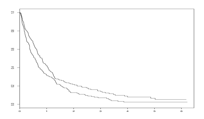
Figure 5: MRC RE01 study. Kaplan Meier plot, control group (green curve) and IFN group (blue curve).

As an illustration, we reconsider the kidney cancer data described in White and Royston, (2009). These data are from the MRC RE01 study that was a randomised controlled trial comparing interferon-$\alpha$ (IFN) treatment with the best supportive care and hormone treatment with medroxyprogesterone acetate (control) in patients with metastatic renal carcinoma. We use the same 347 patients as in White and Royston (2009). In this illustrative analysis we consider only the first 30 months of follow up. The median follow-up time was 242 days, and 85% of the patients died within the considered time frame. The two Kaplan-Meier estimates in Figure 5 contain all the available information about the treatment effect. IFN treatment seems superior to the standard treatment (control), although a supremum test comparing the two survival curves results in a non-significant p-value of 0.09. The score process plot of Lin et al., (1993) was calculated using the R-package timereg (Martinussen and Scheike,, 2006), giving no evidence against the proportional hazards assumption (P 0.43 according to the supremum test). We therefore fitted the Cox model, giving the estimate $\hat{\beta}=-0.29$ (SE 0.12, P 0.01), showing evidence that the IFN treatment reduces the risk of dying for these patients. The hazard ratio of 0.75 expresses the magnitude of the causal effect, but interpretation is subtle as explained before. As a sensitivity analysis we now assume (5) and (9), and take $Z$ to be Gamma distributed with mean 1 and variance $\theta$. This model fits the observed data equally well and thus cannot be refuted based on the observed data. The parameter $\theta$ expresses the correlation between $T^{0}$ and $T^{1}$ and was chosen to give a Kendall’s $\tau$ of 0.1 and 0.2 corresponding to estimated Kendall’s $\tau$ concerning the correlation between lifetimes for dizygotic and monozygotic Danish twins (Scheike et al.,, 2015). A higher correlation between $T^{0}$ and $T^{1}$, corresponding to a Kendall’s $\tau$ of 0.3, was also considered. Figure 6 displays $\mbox{HR}(t)$ under these three scenarios. It is seen that $\mbox{HR}(t)$ is smaller than 0.75 at all times and decreases with time indicating a stronger treatment effect when comparing the instantaneous risk at time $t$ on treatment versus control for the principal stratum of individuals who would have survived up to time $t$, no matter what treatment. This is more pronounced with the larger correlation. In view of these subtleties of interpretation, in this section, we will focus on a number alternative ways of describing the treatment effect.

We may alternatively use the Cox model to estimate the relative risk function

$$\mbox{RR}(t)=\frac{P(T\leq t|A=1)}{P(T\leq t|A=0)}=\frac{P(T^{1}\leq t)}{P(T^{0}\leq t)},$$

which can be estimated consistently by

$$\widehat{\mbox{RR}}(t)=\frac{1-\exp{\{-\hat{\Lambda}_{0}(t)e^{\hat{\beta}}\}}}{1-\exp{\{-\hat{\Lambda}_{0}(t)\}}},$$

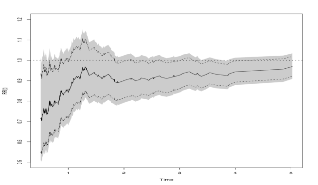
Figure 7: MRC RE01 study. IFN treatment vs control treatment. Estimate of relative risk $\mbox{RR}(t)$ along with 95% pointwise confidence bands (dashed curves) and 95% uniform bands (shaded area).

where $\hat{\beta}$ is the Cox partial likelihood estimator and $\hat{\Lambda}_{0}(t)$ is the corresponding Breslow estimator. This estimate, along with 95% pointwise and uniform confidence bands, is displayed in Figure 7, where we see that the estimated relative risk function is below 1 at all times, in favour of the IFN treatment. For instance, it is seen that the relative risk at one year is estimated to be approximately 0.85, and, judging from the 95% confidence bands (dashed curves), this is close to being significant. A uniform test over the considered time span is also close to being significant judging from the 95% uniform confidence bands.

Another way of quantifying the treatment effect is by using the restricted mean survival time (RMST) (Uno et al.,, 2014; Zhao et al.,, 2016). The RMST up to time $t$ is defined as $\mbox{RMST}(t)=E\{\mbox{min}(T,t)\}$. This is the area under the survival curve of $T$ up to time $t$ and can easily be estimated using the corresponding Kaplan-Meier curve up to time $t$ (see Zhao et al., (2016) for details on inference). Contrasts of the $\mbox{RMST}(t)$ corresponding to different (randomised) treatment groups therefore carry a causal interpretation. The restricted mean time lost, $\mbox{RMTL}(t)$ is defined as $t-\mbox{RMST}(t)$. Here, the ‘months of life lost up to 30 months’ is given by $\mbox{RMTL}(30)$ and estimated to 17.3 for the IFN treatment and to 19.8 for the control treatment. The ratio of these two (IFN vs control) is 0.87 (95% CI, 0.70 to 1.04). Thus, on IFN treatment there is a 13% less loss of lifetime compared to the control treatment during the first 30 months of follow up.

We also fitted Aalen’s additive hazard model

$$\lambda(t;A,V)=\beta_{0}(t)+\psi(t)A+\beta_{1}(t)^{T}V,$$ (12)

where $V$ includes days from metastasis to randomization (log-transformed), WHO performance status (0, 1 and 2; with group 0 and 1 collapsed into one group), and Haemoglobin (g/dl). As the treatment variable $A$ is independent of the other covariates, the above Aalen model is collapsible meaning that the interpretation of $\psi(t)$ is the same in the conditional and marginal model. The Cox model does not have this property. Model (12) appeared to fit the data well, using the tools described in Chapter 5 in Martinussen and Scheike, (2006); specifically no interaction between the treatment indicator and the baseline risk factors was found. We estimated $\hat{\Psi}(t)=\int_{0}^{t}\psi(s)ds$ both from the conditional model and the marginal model, and the two estimators were almost identical, which, as pointed out, should be the case if model (12) is correctly specified. Using model (12), we next tested the null hypothesis $\psi(t)=\psi$ of a constant effect (P 0.58), which was subsequently estimated to be $\hat{\psi}=-0.02$ (SE, 0.009). If $T^{0}\perp\!\!\!\perp T^{1}|V$ (or if the addition of additional variables $Z$ conditional on which $T^{0}$ and $T^{1}$ become independent, does not change the additive structure of the model), then this is also the causal hazard difference. This would mean that over the course of the follow-up, an average of approximately 2 additional deaths will occur for each month of follow-up in each 100 persons under the control treatment alive at the start of the month and who would also be alive under the IFN treatment, compared with each 100 IFN treated persons alive at the start of the month and who would also be alive under the control treatment. As suggested before, the assumption that $T^{0}\perp\!\!\!\perp T^{1}|V$ is implausible however.

4.2 Gastrointestinal tumour study

Stablein and Koutrouvelis, (1985) presented survival data from a randomized clinical trial on locally unresectable gastric cancer. Half of the total 90 patients were assigned to chemotherapy, and the other half to combined chemotherapy and radiotherapy. It was suggested that there was superior survival for patients who received chemotherapy, but only in the first year or so. The same application was considered by Collett, (2015) p. 386-389. For illustrative purposes we consider here the first 720 days of follow up corresponding to the two first time periods considered by Collett, (2015). Figure 8 displays the Kaplan Meier curves corresponding to the two groups, and shows that the survival curves become close at the end of the considered time interval. Applying a Cox regression model with time-by-treatment-interaction, allowing for separate HR’s before and after 1 year of follow-up gives estimated HR’s (Combined vs chemotherapy) of 2.40 (95% CI; 1.25, 4.63) in the first year and 0.78 (95% CI; 0.34,1.76) thereafter (the supremum score process test of Lin et al. (1993) gave no convincing evidence against these two models, with P 0.07 in the first interval and P 0.26 in the second interval). Thus one might be tempted to conclude that the chemotherapy is beneficial in the first year only, and that there might even be a reverse effect afterwards, see Collett, (2015) for a similar analysis and conclusion. However, arguing based on the two hazard ratios is subtle as we have shown. If chemotherapy is more effective then there will be more and more frail subjects in that group making the interpretation of hazard function difficult. We illustrate this using the two estimated hazard ratios and taking the frailty variable to be Gamma distributed mean and variance equal to $\theta$ corresponding to a Kendall’s $\tau$ of 0.3. Figure 9 displays the estimated $\lambda(t,A=1,Z)/\lambda(t,A=0,Z)$ which is seen to depend on time, being larger than 2.4 and increasing towards 3.7 in the first year and, after the change-point (1 year), starting at around 1.2 and then decreasing but being larger than 1 at all times.

5 Concluding Remarks

We have argued that the treatment effect in a proportional hazards model carries a causal interpretation, but that its interpretation is subtle. The proportional hazards assumption does not express, for instance, that treatment works equally effectively at all times, as the hazard ratio at a given time mixes differences between treatment arms due to treatment effect as well as selection. The danger of over interpreting hazard ratios become most pronounced when the hazard ratio is not constant over time (e.g. when the hazard ratio is below 1 for some time and then becomes 1). We have argued that this cannot be interpreted as implying that treatment effectiveness disappears after some time. In our opinion, this is the source of much confusion, and a real concern. Non-constant hazard ratios are indeed fairly common in real life because the proportional hazards assumption is a rather unstable assumption in the following sense. Even when valid in some population, this assumption is likely to fail in subgroups of that population (e.g. if one studies men and women separately), and vice versa. This makes the assumption, at best, an approximation in practice.

We have suggested possibilities to estimate hazard ratios that are causally interpretable because they compare intensities at a given time $t$ with and without treatment for the same patient population: those who would survive that time, no matter what treatment. Inferring such hazard ratios necessitates a sensitivity analysis, however. Furthermore, they have the disadvantage of describing the effect for an unknown subgroup of the population. A better strategy in practice, when interest lies in the dynamic aspects of a treatment, is therefore to design the study such that the collected data provide immediate insight into the dynamic aspects of treatment (e.g. by modifying treatment assignments over time).

Appendix A

A.1 Binary frailty variable

Let $Z$ be binary, for instance $P(Z=0.2)=0.2$ and $P(Z=1.2)=0.8$, low and high risk groups, then $E(Z)=1$, and similar results as in the Gamma-distribution case (Section 3.1) are obtained. In this binary case, the Laplace transform is

$$\phi_{Z}(u)=0.2e^{-0.2u}+0.8e^{-1.2u}.$$

Therefore

$$\mbox{HR}_{Z}(t)\frac{g_{Z}(e^{-\Lambda(t,a=1)})}{g_{Z}(e^{-\Lambda(t,a=0)})}=\frac{\lambda(t;a=1)}{\lambda(t;a=0)},$$

where

$$g_{Z}(u)=\{D\log{(\phi_{Z})}\}\{\phi_{Z}^{-1}(u)\},$$ (13)

which is an increasing function. Hence, if we take $\beta_{1}<0$ and $\beta_{2}=0$, then again

$$\mbox{HR}_{Z}(t)<1$$

for all $t$.

A.2 Frailty model arising by marginalization

It was shown in Section 3.1 that one can always pick a DGP $\lambda(t;A,Z)$ so that the Cox model holds marginally, only conditioning on the observed $A$. Rename $Z$ to $Z_{1}$. We show now that similarly we can also pick a DGP $\lambda(t;A,Z_{1},Z_{2})$ so that it marginalizes to $\lambda(t;A,Z_{1})$ that further marginalizes to $\lambda(t;A)$, the latter being the Cox model. For ease of calculations, let

$$\lambda(t;A,Z_{1},Z_{2})=Z_{2}\lambda^{*}(t;A,Z_{1})$$

with $Z_{2}$ being Gamma distributed with mean and variance equal to 1, and independent of $Z_{1}$ and $A$. Similar calculations as those in Section 3.1 gives the following expression

$$\lambda(t;A,Z_{1},Z_{2})=Z_{1}Z_{2}\lambda_{0}(t)e^{\beta A}\exp{\bigl{[}\Lambda_{0}(t)e^{\beta A}+Z_{1}\{\exp{\{\Lambda_{0}(t)e^{\beta A}}-1\}\bigr{]}}$$ (14)

Hence, if the DGP is governed by (14) then model (4), with $\nu=\infty$, and the marginal Cox model, only conditioning on $A$, are also correctly specified.

A.3 Selection and Cox model

Assume that the Cox model $\lambda(t;A)$ is correctly specified. Will there always be selection? The answer is yes. The Cox model induces randomness as

$$\Lambda_{0}(T)=e^{-A\beta}V,$$

where $V$ is exponentially distributed with mean 1. But then

$$E(V|T>t,A=a)=E(V|V>e^{a\beta}\Lambda_{0}(t),A=a)=1+e^{a\beta}\Lambda_{0}(t).$$

If $e^{\beta}<1$ then

$$E(V|T>t,A=1)<E(V|T>t,A=0).$$

A.4 A DGP with $\mbox{HR}(t)$ and $\mbox{HR}_{Z}(t)$ being different

Let $Z$ be Gamma distributed with mean $1-\alpha$, $\alpha\in(0,1)$, and variance $1$, and let $V_{0}$ and $V_{1}$ be independent Gamma distributed with mean $\alpha$ and variance $1$. Exposure $A$ is binary with $P(A=1)=1/2$. Generate data as follows: $T^{0}=V_{0}+Z,$ $T^{1}=e^{-\beta}(V_{1}+Z)$ and $T=(1-A)T^{0}+AT^{1}.$ Condition (5) holds, and the marginal Cox model is also correctly specified. But in this case $\mbox{HR}(t)\neq\mbox{HR}_{Z}(t)$, and it also easily seen that $\mbox{HR}_{Z}(t)$ depends on $Z$. Different values of $\alpha$ results in different values of Kendall’s $\tau$ thus controlling the correlation between $T^{0}$ and $T^{1}$.

A.5 Hazard differences

We assume (5) and (10). Then

$$\lim_{h\rightarrow 0}P(t\leq T^{1}<t+h|T^{0}\geq t,T^{1}\geq t)=\psi(t)+\frac{E\{\omega(t,Z)e^{-2\int_{0}^{t}\omega(s,Z)\,ds}\}}{E\{e^{-2\int_{0}^{t}\omega(s,Z)\,ds}\}}$$

and

$$\lim_{h\rightarrow 0}P(t\leq T^{0}<t+h|T^{0}\geq t,T^{1}\geq t)=\frac{E\{\omega(t,Z)e^{-2\int_{0}^{t}\omega(s,Z)\,ds}\}}{E\{e^{-2\int_{0}^{t}\omega(s,Z)\,ds}\}}$$

and therefore

$$\psi(t)=\lim_{h\rightarrow 0}P(t\leq T^{1}<t+h|T^{0}\geq t,T^{1}\geq t)-\lim_{h\rightarrow 0}P(t\leq T^{0}<t+h|T^{0}\geq t,T^{1}\geq t).$$

Figure 1: Simulation study. Plot of $\mbox{HR}_{Z}(t)$.

Figure 3: $\mbox{HR}(t)$ in scenarios with $e^{\beta}=0.5$ and with Kendall’s $\tau$ equal to 0, 0.04, 0.2, 0.49, 0.83 and 0.98 (starting from top with $\tau$ equal to 0, corresponding to independence between $T^{0}$ and $T^{1}$).

Figure 4: Simulation study. Estimated cumulated regression coefficient and 95% pointwise confidence bands obtained from fitting the Aalen additive hazards model.

Figure 6: MRC RE01 study. Estimated $\mbox{HR}(t)$ with Kendall’s $\tau$ equal to 0.3 (dotted curve), 0.2 (broken curve) and 0.1 (full curve). Horizontal line corresponds to the Cox hazard ratio of 0.74.

Figure 8: Gastrointestinal tumour study. Kaplan-Meier plot, chemotherapy (full curve) and combined therapy (broken curve).

Figure 9: Gastrointestinal tumour study. Plot of $\lambda(t;A=1,Z)/\lambda(t;A=0,Z)$ based on $\eqref{Cox_AZ}$ with change-point at 1 year and the frailty variable being Gamma distributed with mean 1 and variance so that Kendall’s $\tau$ is equal to 0.3. Dashed curves show the estimated regression coefficients based on the change-point Cox analysis. Combined therapy vs chemotherapy.

References

- Aalen et al., (2015) Aalen, O. O., Cook, R. J., and Røysland, K. (2015). Does cox analysis of a randomized survival study yield a causal treatment effect? Lifetime Data Anal, 21(4):579–93.
- Collett, (2015) Collett, D. (2015). Modelling Survival Data in Medical Research. CRC Press, Boca Raton.
- Hernán, (2010) Hernán, M. (2010). The hazards of hazard ratios. Epidemiology (Cambridge, Mass.), 21(1):13–15.
- Lin et al., (1993) Lin, D. Y., Wei, L. J., and Ying, Z. (1993). Checking the Cox model with cumulative sums of martingale-based residuals. Biometrika, 80:557–572.
- Martinussen and Scheike, (2006) Martinussen, T. and Scheike, T. H. (2006). Dynamic Regression Models for Survival Data. Springer-Verlag, New York.
- Martinussen and Vansteelandt, (2013) Martinussen, T. and Vansteelandt, S. (2013). On collapsibility and confounding bias in cox and aalen regression models. Lifetime Data Anal, 19(3):279–96.
- Rubin, (2000) Rubin, D. B. (2000). Causal inference without counterfactuals: Comment. Journal of the American Statistical Association, 95(450):435–438.
- Scheike et al., (2015) Scheike, T. H., Holst, K. K., and Hjelmborg, J. B. (2015). Measuring early or late dependence for bivariate lifetimes of twins. Lifetime Data Anal, 21(2):280–99.