The time evolution of the Milky Way’s oxygen abundance gradient

Abstract

We study the evolution of oxygen abundance radial gradients as a function of time for the Milky Way Galaxy obtained with our Mulchem chemical evolution model. We review the recent data of abundances for different objects observed in our Galactic disc. We analyse with our models the role of the growth of the stellar disc, as well as the effect of infall rate and star formation prescriptions, or the pre-enrichment of the infall gas, on the time evolution of the oxygen abundance radial distribution. We compute the radial gradient of abundances within the disk, and its corresponding evolution, taking into account the disk growth along time. We compare our predictions with the data compilation, showing a good agreement. Our models predict a very smooth evolution when the radial gradient is measured within the optical disc with a slight flattening of the gradient from $\sim-0.057$ dex kpc^-1 at $z=4$ until values around $\sim-0.015$ dex kpc^-1 at $z=1$ and basically the same gradient until the present, with small differences between models. Moreover, some models show a steepening at the last times, from $z=1$ until $z=0$ in agreement with data which give a variation of the gradient in a range from $-0.02$ to $-0.04$ dex kpc^-1 from $t=10$ Gyr until now. The gradient measured as a function of the normalized radius $R/R_{\rm eff}$ is in good agreement with findings by CALIFA and MUSE, and its evolution with redshift falls within the error bars of cosmological simulations.

1 INTRODUCTION

Metals are formed inside stars; therefore it is expected that metal enrichment in the universe should start soon after the formation of the first massive/short-lived stars, whose explosive demise would return to the interstellar medium (ISM) newly synthesized chemical elements heavier than primordial hydrogen and helium. It is thought that these ejecta, mixed with the surrounding gas, would help its cooling and precipitate the appearance of a new generation of stars, giving rise to the cycle of cosmic chemical evolution.

In a more detailed picture, not all the metals are returned to the ISM with the same timescales: elements like oxygen, sulfur, calcium or magnesium are synthesized in high-mass stars and returned to the ISM after only a few million years, while elements like carbon and nitrogen are mainly made by intermediate-mass stars whose lifetimes are much longer, of the order of thousands of million years. In addition, these chemical elements do not return to the ISM in the same way: the first ones do it through explosive events known as core-collapse supernovae (supernovae of Type II) which release about $10^{51}{\rm erg}$ in mechanical energy, while the second ones do it in a much more quiescent manner through the stellar envelope ejection in planetary nebulae events, at velocities of the order of $10\,{\rm km}\,{\rm s}^{-1}$. Finally, an element like iron is mainly produced in close binary systems after a complex evolution, and ejected in thermonuclear explosive events (supernovae of Type Ia) on relatively long timescales. These different ways that the various elements return to the ISM likely lead to different ways of mixing with the surrounding gas and, when the explosive pathway is followed, the possibility will exist that important quantities of metals can leave the galaxies where they were formed, to enrich the intergalactic medium.

These processes are imprinted on the distribution of elemental abundances in galaxies. The absolute quantities of metals which a galaxy (or a region of a galaxy) possesses, the relative abundances of the different elements, and their spatial distribution in a given galaxy are important constraints for the verification of our models and scenarios of the formation and evolution of galaxies. One very effective way of handling and exploiting this information is to confront derived metal abundances at the present time, that is, from the observation of objects whose lifetime is short as compared to the lifespan of a galaxy, with chemical evolution models; then use the most successful models to infer abundances at previous epochs that can be compared with those corresponding to older galaxy populations. Once convergence is achieved, the models can be extrapolated back to even earlier times and predictions can be made which can be contrasted with planned observations or numerical simulations.

One of the best known features of spiral discs is the existence of a radial gradient of abundances (Henry & Worthey, 1999). This gradient was first observed in the Milky Way Galaxy (MWG, see in Shaver et al., 1983), and then in other external galaxies as shown in McCall, Rybski, & Shields (1985); Zaritsky, Kennicutt, & Huchra (1994) and van Zee et al. (1998), and it is now well characterized in our local Universe (Sánchez et al., 2014). It can be interpreted as due to differences in the star formation rate or the gas infall rate across the disc, although other reasons are also possible (see Goetz & Koeppen, 1992, for a detailed review). In order to understand the role of the involved processes, numerical chemical evolution models were developed early (Lacey & Fall, 1983; Diaz & Tosi, 1984; Matteucci & Francois, 1989; Ferrini et al., 1994). Most of them were able to reproduce the present state of our Galaxy, as radial distributions of star formation, gas density, surface density stellar profile and the radial gradient of most common elements (C, N, O, Fe…), however not all of them predict the same evolution with time. In fact, as Koeppen (1994) explained, the radial abundance gradients may be only modified by inflows or outflows of gas, and, besides the possible variations of the initial mass function (IMF) or stellar yields along the galactocentric radius, the only way to change a radial gradient of abundances is to have a star formation rate (SFR) or an infall rate changing with galactocentric radius.

It was demonstrated a long time ago (Lacey & Fall, 1983; Matteucci & Francois, 1989) that an inside-out scenario of formation of discs, as produced by different infall rate of gas along the disc, is necessary to form a negative radial gradient of abundances. However, in order to obtain a value of gradient as observed, it is also necessary to invoke radial flows of gas or variable star formation efficiencies, which should be higher in the inner regions than in the outer ones. Using these assumptions, most models able to reproduce the present state of the solar neighborhood and the Galactic disc as a whole, follow one of two trends: a) It is initially flat and it steepens with time; or b) the gradient is steep, and flattens with time. For example, models from Diaz & Tosi (1984); Chiappini, Matteucci, & Gratton (1997) predict an initially flat radial distribution of abundances which then steepens with time. Conversely, models by Ferrini et al. (1994); Prantzos & Aubert (1995); Mollá, Ferrini, & Díaz (1997); Portinari & Chiosi (2000); Hou, Prantzos, & Boissier (2000) present a steep initial radial abundance gradient which flattens with time. The first scenario is the consequence of the existence of the disc as initial conditions combined with an infall of primordial gas which dilutes the metal enrichment of the disc preferentially in the outer regions. In the second scenario, however, it is the infall of gas which forms the disc and contributes to the metal budget since it proceeds from the halo and is therefore somewhat enriched due to earlier star formation. Grisoni, Spitoni, & Matteucci (2018) explain that “the one-infall model with only inside-out or radial gas inflows predicts a steepening of the gradient with time, whereas the same case adding a variable star formation efficiency predicts a flattening of the gradient with time”. Therefore, it seems evident that the radial gradient of abundances observed in spirals is dependent upon the scenario of formation and evolution of the disc.

From an observational perspective, the question of appropriate data sets against which to compare has been debated vigorously. In Mollá, Ferrini, & Díaz (1997) we analysed the existing data concerning this question for the MWG with three types of data: 1) planetary nebulae (PNe) of different masses (that is, different ages) to analyse the oxygen abundance radial distributions at different times; 2) open and globular clusters (OC and GC, respectively), to estimate the global metallicity in objects of different ages; 3) stellar abundances. Each data set has its own problems for determining the time evolution of the radial gradient. PNe are useful for estimating the radial gradient of oxygen, an element not modified by nucleosynthesis in their progenitor stars . (2003) analysed the early data around this question, showing a radial gradient steeper than the one seen in the present time, although, due to the error bars, the observational points mixed with the Hii region’s data in the plot of O/H vs. galactocentric radius $R$. Besides the large errors, the problem with PNe is that to estimate their galactocentric distances and their stellar masses (and therefore their ages) is a process with large uncertainties.

The OC problems arise from the necessary classification of thin or thick disc or even halo populations, which requires a previous kinematic study, before their use to determine a radial distribution in metallicity. Furthermore, the age determination comes from a fit of their spectra to stellar models which depend on metallicity and age simultaneously, which added to differences depending on the use of LTE or NLTE models, may be uncertain. For these reasons, OC age determination is not an easy task, although the error bars are smaller than for PNe. The box enclosing the data corresponding to these objects basically falls in the same region as the young stars in a plot of [Fe/H] vs. $R$.

The estimates of age and metallicity for GC seem less problematic since it is assumed that they form as a single stellar population.. Ages and metallicities for stars in a GC are therefore known more precisely than those in OC. Based on these data, we concluded more than 20 years ago (Mollá, Ferrini, & Díaz, 1997) that the radial gradient of abundances in MWG seems steeper in the past and has been flattening with time until arriving to the present value. However, these old objects may also be part of the thick disc or the halo populations. As for the OC, the kinematic information is essential to determine their group and therefore to know if the corresponding data may be included in the study of time evolution of the radial distributions of disc abundances. In Mollá & Díaz (2005)—hereinafter MD05—we presented 440 chemical evolution models, with 44 different galaxy masses and 10 possible star formation efficiencies in each one. From a MWG-like model, the radial gradient of oxygen abundances is $\sim-0.20$ dex kpc^-1 at $z=2$, which flattens with time until reaching the present time ($z=0$) value $\sim-0.05$ to $-0.06$ dex kpc^-1. This behavior was in agreement with observations available at the time.

In recent years, however, new datasets and results from cosmological simulations have appeared. In the light of these results, we think that it is time to revise the question of the evolution of the radial gradient of abundances.

In the present work we use the MULCHEM models, which are based in those ones from Mollá & Díaz (2005). They are 1D models in which we do not include radial gas flows, as it was done in Cavichia et al. (2014). There it was found that the model with radial gas flows induced by the Galactic bar increases the SFR in the bar/bulge-disc transition region. A slight difference in elemental abundances is also noted; the model with gas flows predicts a flatter radial distribution in the outer disc but the change is so small that it probably cannot be detected by the current observations.

Another mechanism recently included in other models from the literature is (stellar) radial migration, usually invoked as one of the secular processes that may modify the disc. It is driven by transient spiral patterns which rearrange the angular momentum (see Minchev et al., 2012; Daniel & Wyse, 2018, for a detailed explanation). In this way, spiral arms may induce the migration of stars away from their location of birth, resulting in variations in the stellar composition with galactocentric radius. The process may explain the existence of the large observed dispersions in the distribution of stellar metallicities at a given galactocentric distance, and, as a certain number of stars more metal-rich than expected will appear in the outer regions, resulting in a flattening of the radial distribution of stellar abundances. Thus, Sánchez-Blázquez et al. (2009) or Minchev et al. (2012), including radial migration in their cosmological simulations, obtained a stellar metallicity radial gradient which flattens outside. Ruiz-Lara et al. (2017b) also demonstrate how metallicity gradients for galaxies with different break types change when considering where stars are born and where they have migrated. They find an average change in $\Delta$[M/H] of 0.05 dex/inner disc scale-length comparing galaxies with radial migration and accretion of stars and galaxies with relatively steep metallicity gradient and under the influence of galaxy mergers which drive much of the migration. Following these simulations, it is expected that the migration affects more to the oldest stellar populations (see Fig. 22 from Sánchez-Blázquez et al., 2009).

Radial migration is not included in our models. In our scenario, the Galaxy has a halo or proto-galaxy and a thin disc. It is necessary to have the kinematic information of stars to follow their movements, which would require the development of a new code. To include all details of the complex structure of the Galactic disc (thin and thick discs, bar, spiral arms, flares) is beyond the scope of this work. We have undertaken a project to include these 2D structures in our new model which will be published in the near future. Here we try to understand the evolution of the MWG in a more generic way in order to apply the same type of model in other external galaxies. Moreover, the proportion of discs showing a flattening at the outer regions is only of $\sim 20-30$% (Sánchez-Blázquez et al., 2009; Ruiz-Lara et al., 2017a) and therefore radial migration is not an essential mechanism to explain the underlying radial distributions of discs. It will be necessary, however, to take possible stellar migration into account when we compare the model results with the data, mainly when old OC or stars are used, and with object located in the outer regions of disc, when/where the migration might be more important, since in this case their abundances may not represent the one of the local gas at their formation time.

We give a summary of the observations related to different age objects in MWG in Section 2. For our study, we have generated a new suite of chemical evolution models, described in Section 3, where we have revised all the necessary code inputs. In Section 4, we will analyse the results corresponding to the MWG model, comparing with data compiled in Section 2. In Section 5 we present a discussion about the evolution of the radial gradient and the conclusions are given in Section 6.

2 OBSERVATIONAL DATA FOR MWG

We have done a search of data from the literature that we here divide as corresponding to the present time (Hii regions and young stars) or to past times (PNe, OC and stars of different ages).

2.1 Present Day Data

2.1.1 Nebular data: Hii data.

We summarize here our analysis of different recent of Hii data sets from several works in the literature. Rudolph et al. (2006) present data for Hii regions at galactocentric distances of R $\sim$ 10-15 kpc, which have been observed in the far IR emission lines of [O III] (52 $\mu$m, 88 $\mu$m), [N III] (57 $\mu$m), and [S III] (19 $\mu$m) using the Kuiper Airborne Observatory. In total, 168 sets of observations of 117 Hii regions. The new analysis includes an update of the atomic constants (transition probabilities and collision cross sections), recalculation of some of the physical conditions in the Hii regions ($n_{e}$ and $T_{e}$), and the use of new photo-ionization models to determine stellar effective temperatures of the exciting stars.

Balser et al. (2011) measure radio recombination line and continuum emission in 81 Galactic Hii regions at Galactocentric radii of 5 to 22 kpc and also sample the Galactic azimuth range $330-60^{\circ}$. Using their highest quality data (72 objects) they measured the electron temperature and derived the oxygen abundance from the calibration given in Shaver et al. (1983):

$$12+\log({\rm O/H})=9.82(\pm 0.02)-1.49(\pm 0.11)T_{\rm e}/10^{4},$$ (1)

thus deriving an O/H Galactocentric radial gradient of -0.0383$\pm$ 0.0074 dex kpc^-1. Combining these data with a similar survey made with the NRAO 140 Foot telescope, they get a radial gradient of $-0.0446\pm 0.0049$ dex kpc^-1 for a larger sample of 133 nebulae.

Fernández-Martín et al. (2017) have done observations with the William Herschel Telescope in the Los Muchachos Observatory (La Palma) for 9 Hii regions. They joined them to other literature data, and reanalysed all in a homogeneous manner. In total they obtain abundances for 23 objects, covering the galactocentric radius from 11 kpc to 18 kpc i.e., in the outer disc. They measure the radial gradient for O, N, S, Ar and also for He and N/O, obtaining the following values: $-0.0525(\pm 0.009$), $-0.080(\pm 0.019)$, $-0.106(\pm 0.006$), $-0.074(\pm 0.006$), $-0.0005(\pm 0.0019$) and $-0.041(\pm 0.006$)  dex kpc^-1, respectively. Similarly, Esteban et al. (2017) analyse Hii regions also for the outer regions of disc using the Gran Telescopio Canarias (GTC) telescope, finding a radial gradient for O of $-0.0399$ dex kpc^-1.

We have combined all these data in Fig. 1, panel a) and performed a binning of all data to have a point for each kpc. These results are given in Table 1, column 2, with the corresponding statistical error resulting from the binning process. We have data from $R=0$ out to 18 kpc. It is possible that, in the process of binning, data coming from different samples (obtained in some cases with different techniques) are adding a systematic error. However, we consider that this systematic error is already taken into account in the shown dispersion of data and the corresponding statistical error obtained in the binning of points. This statement is also valid for the following subsections, where we discuss other objects that are relevant to obtaining oxygen abundances.

Table 1: Radial distribution of oxygen abundances for different object binned from data of different authors.

	Hii	Cepheid	PNe	Young	Intermediate	Old	Young	Intermediate	Old
	Regions	Stars		age OC	age OC	age OC	age Stars	age Stars	age Stars
R	12+log(O/H)
(kpc)	(dex)
0	8.90 $\pm$ 0.12
1			8.67 $\pm$ 0.12
2			8.72 $\pm$ 0.12
3	8.61 $\pm$ 0.28	9.02 $\pm$ 0.05	8.72 $\pm$ 0.10
4	8.64 $\pm$ 0.23	8.89 $\pm$ 0.15	8.72 $\pm$ 0.12				8.55 $\pm$ 0.05	8.55	8.55
5	8.79 $\pm$ 0.11	9.02 $\pm$ 0.10	8.68 $\pm$ 0.11	8.95 $\pm$ 0.07			8.44 $\pm$ 0.23	8.57 $\pm$ 0.10	8.40 $\pm$ 0.10
6	8.78 $\pm$ 0.15	8.88 $\pm$ 0.07	8.62 $\pm$ 0.09	8.81 $\pm$ 0.08			8.69 $\pm$ 0.09	8.70 $\pm$ 0.06	8.58 $\pm$ 0.07
7	8.76 $\pm$ 0.10	8.74 $\pm$ 0.06	8.70 $\pm$ 0.07	8.75 $\pm$ 0.11	8.97 $\pm$ 0.05		8.67 $\pm$ 0.06	8.68 $\pm$ 0.05	8.62 $\pm$ 0.06
8	8.53 $\pm$ 0.09	8.72 $\pm$ 0.06	8.64 $\pm$ 0.08	8.61 $\pm$ 0.08	8.68 $\pm$ 0.10	8.80 $\pm$ 0.14	8.66 $\pm$ 0.05	8.65 $\pm$ 0.05	8.62 $\pm$ 0.06
9	8.62 $\pm$ 0.09	8.70 $\pm$ 0.06	8.64 $\pm$ 0.13	8.70 $\pm$ 0.07	8.69 $\pm$ 0.08	8.61 $\pm$ 0.11	8.62 $\pm$ 0.05	8.58 $\pm$ 0.06	8.55 $\pm$ 0.07
10	8.39 $\pm$ 0.10	8.68 $\pm$ 0.06	8.57 $\pm$ 0.10	8.61 $\pm$ 0.09	8.80 $\pm$ 0.10	8.70 $\pm$ 0.05	8.61 $\pm$ 0.07	8.63 $\pm$ 0.07	8.61 $\pm$ 0.08
11	8.40 $\pm$ 0.08	8.61 $\pm$ 0.07	8.47 $\pm$ 0.12	8.55 $\pm$ 0.14	8.49 $\pm$ 0.11	8.56 $\pm$ 0.09	8.64 $\pm$ 0.06	8.69 $\pm$ 0.08	8.63 $\pm$ 0.14
12	8.43 $\pm$ 0.07	8.52 $\pm$ 0.08	8.71 $\pm$ 0.12	8.40 $\pm$ 0.09	8.50 $\pm$ 0.08	8.65 $\pm$ 0.13	8.57 $\pm$ 0.07	8.54 $\pm$ 0.07
13	8.38 $\pm$ 0.09	8.49 $\pm$ 0.08	8.33 $\pm$ 0.12	8.60 $\pm$ 0.10	8.44 $\pm$ 0.10	8.64 $\pm$ 0.05	8.56 $\pm$ 0.08	8.54 $\pm$ 0.08
14	8.33 $\pm$ 0.13	8.53 $\pm$ 0.09	8.55 $\pm$ 0.13	8.60 $\pm$ 0.11	8.55 $\pm$ 0.06		8.48 $\pm$ 0.09
15	8.13 $\pm$ 0.11	8.48 $\pm$ 0.13	8.53 $\pm$ 0.24	8.65 $\pm$ 0.06			8.63 $\pm$ 0.13
16	8.16 $\pm$ 0.07	8.41 $\pm$ 0.13			8.38 $\pm$ 0.05	8.53 $\pm$ 0.05
17	8.17 $\pm$ 0.09	8.32 $\pm$ 0.05					8.53 $\pm$ 0.05
18	7.91 $\pm$ 0.16				8.47 $\pm$ 0.05
19					8.73 $\pm$ 0.05

We give in Table LABEL:grad_OH the radial gradient of oxygen abundances given by different authors. Each reference is in column 1, with the corresponding radial gradient of oxygen abundances in column 2, and the radial range covered in column 3. The resulting radial gradient obtained after the binning process with all points is also given (this work) in that table at the end of each block for each object type.

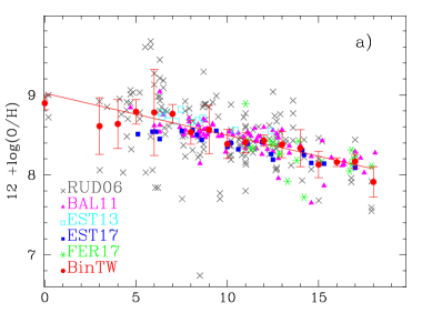
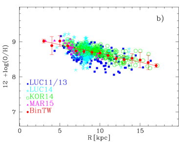
Figure 1: The present time radial distribution of the oxygen abundances, $12+\log{(\rm O/H)}$, for MWG with data from different authors: a) for Hii regions from Rudolph et al. (2006); Balser et al. (2011); Esteban et al. (2017); Fernández-Martín et al. (2017) (RUD06, BAL11, EST17, FER17 respectively) as labelled in the legend; b) for Cepheids stars from Luck & Lambert (2011); Luck et al. (2013); Luck (2014); Korotin et al. (2014); Martin et al. (2015) (LU11/13, LU14, KOR14 and MAR15 respectively) as labelled in the legend. Our binned results (BinTW) are shown in both panels as red full dots with the least square straight line plotted over the points in each case.

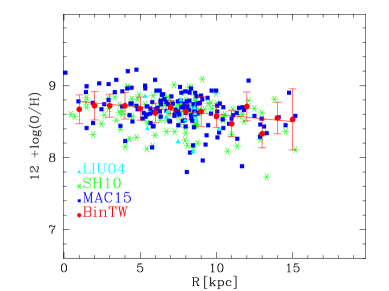
Figure 2: The radial distribution of the oxygen abundances, $12+\log{({\rm O/H})}$, for PNe in the MWG. Data are from Liu et al. (2004); Stanghellini & Haywood (2010) and Maciel, Costa, & Cavichia (2015), denoted by LIU04, SH10 and MAC15, respectively, as labelled in the legend. Our binned results are shown as red full dots with the least square straight line plotted over the points.

Table 2: Radial gradient of Oxygen abundances from different sets of observational data

Author	Time/age	$\nabla$ [O/H]	radial range	N
	Gyr	(dex kpc-1)	(kpc)
Present time
Hii Regions
RUD06	Present	$-0.0543\pm 0.008$	3–18	151
BAL11	Present	$-0.0446\pm 0.0051$	4–18	81
EST13	Present	$-0.0381\pm 0.0087$	6-13	10
EST17	Present	$-0.0399\pm 0.0044$	5–17	20
FER17	Present	$-0.0525\pm 0.0189$	11-18	22
This work	Present	$-0.048\pm 0.005$	0–18	284
Cepheids
LUCK11/13	Present	$-0.0430\pm 0.0065$	4–17	168
LUCK14	Present	$-0.0225\pm 0.0047$	4–14	815
KOR14	Present	$-0.0529\pm 0.0083$	5-18	271
MAR15	Present	$-0.080\pm 0.010$	3-11	26
This work	Present	$-0.0498\pm 0.05$	3–17	1280
Past time
PNe
LIU04	2-4	$-0.048\pm 0.048$	5–11	12
SH10	all	$-0.024\pm 0.019$	1–15	125
	Type I	$-0.035\pm 0.024$
	Type II	$-0.023\pm 0.005$
	Type III	$-0.011\pm 0.013$
MAC15	2-4	$-0.026\pm 0.006$	0–16	149
This work	2-4	$-0.020\pm 0.050$	0–16	286
Open Clusters
CAR11 $+$ Lit		$-0.049\pm 0.059$	8-14	43
	$\tau\leq 2$	$-0.0210\pm 0.0175$	7–14	39
	$2<\tau\leq 8$	-0.060 $\pm$ 0.041	9-11	2
	$\tau>8$	$+0.005\pm 0.000$	8–12	2
YONG12		$-0.027\pm 0.008$	6–21	39
	$\tau\leq 2$	$-0.085\pm 0.026$	8–13	13
	$2<\tau\leq 8$	-0.0204 $\pm$ 0.008	6-20	24
	$\tau>8$	$-0.083\pm 0.000$	8–11	2
FRIN13		$-0.044\pm 0.019$	7–14	28
	$\tau\leq 2$	$-0.036\pm 0.021$	8-14	22
	$2<\tau\leq 8$	-0.106 $\pm$ 0.032	8-13	5
	$\tau>8$		9	1
CUN16		$-0.031\pm 0.009$	6–17	28
	$\tau\leq 2$	$-0.022\pm 0.017$	6–15	7
	$2<\tau\leq 8$	-0.030 $\pm$ 0.009	8-14	7
	$\tau>8$	$-0.0354\pm 0.045$	8–16	14
MAG17		$-0.027\pm 0.0085$	5-17	10
	$\tau\leq 2$	$-0.116\pm 0.034$	5–7	8
	$2<\tau\leq 8$	-0.060 $\pm$ 0.000	10-17	2
	$\tau>8$			0
This work	$\tau\leq 2$	$-0.030\pm 0.001$	4–15	89
	$2<\tau\leq 8$	-0.027 $\pm$ 0.004	6-20	42
	$\tau>8$	$-0.028\pm 0.016$	8–16	19
Stars
EDV93	$\tau\leq 2$	$-0.019\pm 0.050$	7–9	18
	$2<\tau\leq 8$	$-0.0381\pm 0.020$	6–11	99
	$\tau>8$	$-0.00394\pm 0.025$	4–11	44
CASA11	$\tau\leq 2$	$-0.039\pm 0.004$	4–11	4680
	$2<\tau\leq 8$	$-0.0419\pm 0.003$	4–13	4203
	$\tau>8$	$+0.0076\pm 0.0056$	4–12	1326
BERG14	$\tau\leq 2$	$+0.163\pm 0.122$	7–9	6
	$2.5<\tau\leq 8$	$-0.0642\pm 0.048$	7–10	61
	$\tau>8$	$+0.057\pm 0.422$	7–9	8
AND17	$\tau\leq 2$	$-0.033\pm 0.005$	5–16	151
	$2<\tau\leq 8$	$-0.0253\pm 0.0064$	6–12	273
	$\tau>8$	$+0.0724\pm 0.054$	5–7	51
This work	$\tau\leq 2$	$-0.040\pm 0.018$	4–16	4851
	$2<\tau\leq 8$	$-0.028\pm 0.002$	4–14	4636
	$\tau>8$	$0.005\pm 0.012$	4–12	1429

2.1.2 Stellar data: Cepheids

The best way to obtain abundances for present time from stars is measuring the ones of very young luminous stars such as Cepheids. Luck et al. (2013) derive oxygen abundances for a large sample of Cepheids (103) using the near-IR triplets 777.4 nm and 844.6 nm from an NLTE (Non Local Thermodynamic Equilibrium) analysis. The spectra used in this analysis are the same as those used in Luck et al. (2011) and Luck & Lambert (2011) as the southern Cepheid sample. Distances are taken from these two works. More recently, Luck (2014) obtain an O gradient of $-0.042$ dex kpc^-1 for a set of young luminous stars, which reduces to $-0.033$ dex kpc^-1 for the subsample without Cepheids.

Korotin et al. (2014) also did an NLTE analysis of the IR oxygen triplet for a large number of Cepheid star spectra. Together with the data from Luck et al. (2013) they obtain a gradient of $-0.058$ dex kpc^-1 for O. In turn, Martin et al. (2015) have obtained elemental abundances in 27 Cepheids, the great majority situated within a zone of galactocentric distances ranging from 5 to 7 kpc. The data, combined with data on abundances in the very central part of our Galaxy taken from the literature, show that iron, magnesium, silicon, sulfur, calcium and titanium LTE (Local Thermodynamic Equilibrium) abundance radial distributions, as well as the NLTE distribution of oxygen, reveal a plateau-like structure or even positive abundance gradient in the region extending from the Galactic Centre to about 5 kpc.

Lemasle et al. (2013) took high-resolution spectra to measure the abundances of several light (Na, Al), $\alpha$ (Mg, Si, S, Ca), and heavy elements (Y, Zr, La, Ce, Nd, Eu) in a sample of 65 Milky Way Cepheids. Combining these results with accurate distances allows us to determine the abundance gradients in the Milky Way. Their data, however, do not include O abundances. The same issue occurs with the new set of homogeneous measurements of Na, Al, and three $\alpha$-elements (Mg, Si, Ca) for 75 Galactic Cepheids obtained by Genovali et al. (2015). These measurements were complemented with Cepheid abundances provided by the same group or available in the literature, resulting in a total of 439 Galactic Cepheids. Accurate galactocentric distances based on near-infrared photometry are also available for all the Cepheids in the sample. They cover a large section of the Galactic thin disc ($4.1\leq R\leq 18.4$ kpc). It is found that these five elements display well-defined linear radial gradients and modest standard deviations over the entire range of Galactocentric distances.

In a similar way to the previous subsection for Hii data, we have used data from the above cited authors (Luck & Lambert, 2011; Luck et al., 2013; Luck, 2014; Korotin et al., 2014; Martin et al., 2015), joined and represented in panel b) of Fig. 1. We have binned all of them into a single distribution, given in Table 1, column 3. We have points between 3 and 17 kpc. As it is shown in Table LABEL:grad_OH, the radial gradient of O abundances is similar for Hii regions and Cepheids stars, with a value $\sim-0.05$ dex kpc^-1.

2.2 Past times

2.2.1 Planetary Nebulae

(2003) did estimates of the time variation of the O/H radial gradient in a sample containing about 240 nebulae with accurate abundances located in the Galactic disc. For most of these nebulae they had O abundances from the samples of Maciel & Quireza (1999) and Maciel & Koppen (1994), although about 40 new nebulae were included. In this case, the radial gradient for PNe associated to the youngest ages (present time) was $\sim-0.06$ dex kpc^-1. These results were consistent with a flattening of the O/H gradient, roughly from $-0.11$ dex kpc^-1 to $-0.06$ dex kpc^-1 during the last 9 Gyr, or from $-0.08$ dex kpc^-1 to $-0.06$ dex kpc^-1 during the last 5 Gyr.

Other PNe data were obtained from Liu et al. (2004), who list elemental abundances for 12 Galactic PNe. Abundance analyses were carried out using both strong collisionally excited lines (CELs) and weak optical recombination lines (ORLs) from heavy element ions. Using the distances from Stanghellini & Haywood (2010, hereinafter SH10), these data give a radial gradient of $-0.048$  dex kpc^-1, in good agreement with the above data.

However, the most recent findings of PNe data give a smooth evolution with time such as in Henry et al. (2010), with only a slight flattening of the gradient, or even a constant value or a steepening with time as in SH10. This last one gives an average radial gradient of $\sim-0.023$  dex kpc^-1. By dividing their sample by types, SH10 found O/H gradients of $-0.035$, $-0.023$ and $-0.011$  dex kpc^-1, for types I, II and III, respectively, of which the first type corresponds to the youngest thin disc PNe and the last one the oldest bin. This implies that the gradient steepens slightly with time.

Maciel & Costa (2013, hereinafter M13) reached a similar conclusion, that the O/H radial gradient is basically the same from 5–6 Gyr ago until now. These authors worked with a large sample of data, and used three different techniques to derive the ages of the progenitor stars. This allowed them to divide the sample in two or more groups according to the ages. They found an average O/H radial gradient of $\sim-0.04$ dex kpc^-1 and conclude that it has not changed appreciably . Therefore, within the uncertainties, the O/H gradients from PNe could be not very different from the gradients observed in younger objects (Hii and Cepheids). Magrini et al. (2016, hereinafter M16) obtain similar results for some nearby spiral galaxies, M 33, M 31, M 81 and NGC 300, from the comparison of the radial distributions of oxygen abundances given by Hii regions and PNe, respectively, without finding any evidence of evolution of the radial gradient with time.

Maciel, Costa, & Cavichia (2015) have compiled a large number of PNe abundances (265) giving a radial gradient of $-0.02$ to $-0.05$ dex kpc^-1. In this case they divided the sample in different groups of height $|z|$ over the disc, associating those with the highest $|z|$ to the lowest mass or oldest objects, in comparison with the closest ones, that will be the youngest. According to this scheme, the radial gradient is $-0.0218$ dex kpc^-1 for the youngest object and $-0.0268$ dex kpc^-1 for the oldest (dividing into two bins with $|z|\leq 600$ or $|z|>600$ pc, respectively). Taking into account that the difference between these above values is not large (smaller than the error bar of the data), we may conclude that the radial gradient of abundances has not changed appreciably in the last 5–8 Gyr. In this work we have joined the data from Liu et al. (2004); Stanghellini & Haywood (2010) and Maciel, Costa, & Cavichia (2015).

From Bland-Hawthorn & Gerhard (2016) the scale height for the thin disc is 220–450 pc. Following Jurić et al. (2008) it is $\sim$ 300 pc, while it is $>700$ pc for the thick disc. More recently, from McMillan (2017), $z_{D,thin}=300$ pc and $z_{D,thick}=900$ pc. Since we are interested in the evolution of the radial gradient in the thin disc and not in the thick disc or the halo, we assume a limit in the height scale to define the thin disc component. Thus, we have selected only objects with $|z|\leq 600$ pc, assuming that these are the true members of the thin disc, and that objects above this height do not pertain to the thin disc, but instead are members of the thick disc or halo. This limit seems to be safe enough, even taken into account the flare of the outer disc. This same assumption is also taken in the subsection 2.2.3 about stellar data. Curiously, when we constrain our sample to this height above the disc, the galactocentric distances of the selected PNe are all within R$<15$ kpc, that is they are surely located within the thin disc at the present time. We show O abundances in Fig. 2 and our binned abundances (column 4 from Table 1). We have points in the radial range between R=0 and 16 kpc. For our points we have computed the radial gradient as $\sim-0.020$ dex kpc^-1.

Most of the PNe have ages $<4$ Gyr (Maciel & Costa, 2013) and therefore the radial migration is not expected to be important when considering PNe. See the simulations of Kubryk, Prantzos, & Athanassoula (2015), in particular their Fig. 6, showing that for the youngest stars ($<4$ Gyr old) the effect of radial migration is very small.

2.2.2 Open clusters

For OC practically all data, from earlier publications (Friel et al., 2002; Chen, Hou, & Wang, 2003; Magrini et al., 2009) to the more recent (Frinchaboy et al., 2013; Cunha et al., 2016), arrive at the same conclusion: the radial gradient of stellar metallicity was steeper in the past than now. However, most of data referring to OC estimate this gradient with Fe abundances or with a metallicity index as [M/H]. Friel et al. (2002); Friel, Jacobson, & Pilachowski (2010) measured an [Fe/H] gradient of $-0.080$ dex kpc^-1 for the older OC and $-0.02$ dex kpc^-1 for the younger ones. Chen, Hou, & Wang (2003) obtained the same results.

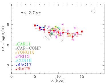
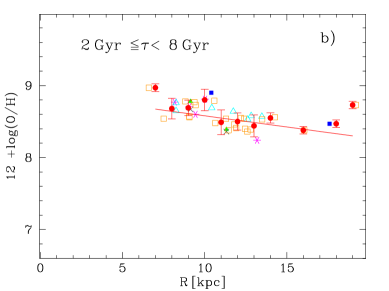
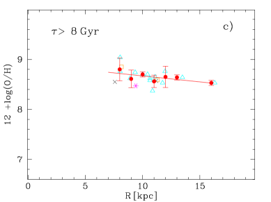
Figure 3: The radial distribution of the oxygen abundances, $12+\log{\rm(O/H)}$, for MWG OC of: a) young age; b) intermediate age; and c) old age, with data from different authors: Pancino et al. (2010); Carrera & Pancino (2011); Yong, Carney, & Friel (2012); Frinchaboy et al. (2013); Cunha et al. (2016); Magrini et al. (2017) –as PAN10 and CAR11, FRI13, YONG12, CUN16 and MAG17, respectively– as labelled in panel a). Our binned results are shown as red full dots in all panels with the least square straight line above the points.

Similarly, Pancino et al. (2010); Carrera & Pancino (2011); Andreuzzi et al. (2011); Yong, Carney, & Friel (2012); Frinchaboy et al. (2013); Reddy, Lambert, & Giridhar (2016); Cunha et al. (2016); Reddy, Giridhar, & Lambert (2013); Netopil et al. (2016); Jacobson et al. (2016); Cantat-Gaudin et al. (2016); Spina et al. (2017); Magrini et al. (2017) find that older open clusters use to show a steeper radial gradient that the youngest ones. This result changes when objects are located at long galactocentric distances, well outside of the optical radius i.e., $R>15$ kpc. This is specially important when we will confront the radial gradient of the disc at early times, as predicted by models (next section), which represent a spiral disc still growing, with data which maybe form part of the halo or the thick disc. In this case a flat radial gradient as observed is expected. We give a warning about this distinction when the study of the radial gradient of spiral discs is addressed.

Although most of works are devoted to the metallicity, measured as [Fe/H] or [M/H], some of them estimate the O abundances for OC of different ages. This way, Pancino et al. (2010); Carrera & Pancino (2011) present high-resolution (R $\sim$ 30 000), high-quality (S/N $\geq$ 60 per pixel) spectra for twelve stars in four open clusters with the fiber spectrograph FOCES, at the 2.2 m Calar Alto Telescope in Spain. They employ a classical equivalent-width analysis to obtain accurate abundances of sixteen elements: Al, Ba, Ca, Co, Cr, Fe, La, Mg, Na, Nd, Ni, Sc, Si, Ti, V, and Y. They also derived oxygen abundances by means of spectral synthesis of the 6300 Å forbidden line. They use a compilation of literature data to study Galactic trends of [Fe/H] and [$\alpha$/Fe] with galactocentric radius, age, and height above the Galactic plane. They find no significant trends, but some indicate a flattening of [Fe/H] at large galactocentric radii, (and also for younger ages in the inner disc). They also detect a possible decrease in [Fe/H] with $|z|$ in the outer disc, and a weak increase in [$\alpha$/Fe] with galactocentric radius.

Yong, Carney, & Friel (2012) have measured chemical abundances for nine stars in the old, distant open clusters Be18, Be21, Be22, Be32, and PWM4. Combining these data with literature, they do a compilation of chemical abundance measurements in 49 clusters. They confirm that the metallicity gradient in the outer disc is flatter than the gradient in the vicinity of the solar neighborhood. They also find that OCs in the outer disc are metal-poor, with enhancements in the ratios [$\alpha$/Fe] and perhaps [Eu/Fe]. All elements show negligible or small trends between [X/Fe] and distance ($\leq 0.02$ dex kpc^-1), except for some elements for which there is a hint of a difference between the local (R $<$ 13 kpc) and distant (R$>$ 13 kpc) samples, which may have different trends with distance. There is no evidence for significant abundance trends versus age (with an age gradient $\leq 0.04$ dex Gyr^-1). They give the O abundances for 39 of these OC, which we use here.

Frinchaboy et al. (2013) also measured [Fe/H] for globular clusters of different ages and they also give abundances for $\alpha$-elements as [$\alpha$/Fe]; although not exactly the same as [O/Fe], we use it to estimate [O/H]. Cunha et al. (2016) obtained [Fe/H] and [O/Fe] for their sample of OC, too. Although they give the radial gradients for different ages only for [Fe/H], we may obtain the gradients for [O/H] in a similar way.

Magrini et al. (2017) observed open clusters with ages $\tau>$ 0.1 Gyr. The sample includes several new clusters: NGC 2243, Berkeley 25, NGC 6005, NGC 6633, NGC 6802, NGC 2516, Pismis 18 and Trumpler 23 and four clusters already processed in previous data releases and discussed in previous papers: Berkeley 81, NGC 4815, Trumpler 20, and NGC 6705. Most clusters are younger than 2 Gyr. Only the two outer ones are older than this.

We summarize all data in Fig. 3. As we have for the PNe, we have selected objects located at $|z|<600$ pc, without any other restriction, and have divided the sample into young, intermediate and old objects, with ages lower than 2 Gyr, between 2 and 8  Gyr, and older than 8 Gyr, respectively, as labelled in each panel. For each subsample we have binned the abundances, shown as red dots (as in our previous Fig. 1 and 2), which are in Table 1, columns 5, 6, and 7. The corresponding radial gradients for OC of these authors are in Table LABEL:grad_OH, too. In the first line for each author we give the gradient as given by them, or, the one produced using all objects of their samples. In next lines we give the radial gradients as obtained for us for different age bins, as indicated.

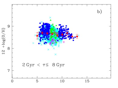
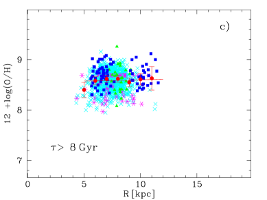
Figure 4: The radial distribution of the O abundances, $12+\log{({\rm O/H})}$, for MWG stars of different ages: a) young ($\tau\leq 2$ Gyr); b) intermediate ($2<\tau\leq 8$ Gyr) and c) old stars ($\tau>8$ Gyr), as indicated in each panel, with data from Edvardsson et al. (1993); Casagrande et al. (2011); Bergemann et al. (2014); Anders et al. (2017), labelled in panel a) as EDV93,CASA11,BER14 and AND17. Our binned results are shown as red full dots in all panels with the least square straight line plotted over the points.

2.2.3 Stellar data

Finally, we have the stellar data, such as those from Edvardsson et al. (1993); Nordström et al. (2004); Casagrande et al. (2011); Bergemann et al. (2014); Xiang et al. (2015). Following most of these authors, stellar abundance data show a flattening of the radial gradient with time . However, for the oldest age bin ($\sim$ 12-13 Gyr old) the radial gradient is usually zero, meaning that the radial gradient started flat, became steeper, and later flattened again.

Anders et al. (2017), from the data for red giants observed by CoRoT and APOGEE, obtain a radial gradient steepening continuously with time, in disagreement with the other authors. Looking at all these data in detail, we find some problems for the precise determination of the radial gradient for the old age bin, since the radial range in which it is measured is extremely short, preventing the reliable measurement of a gradient. Bergemann et al. (2014) and Xiang et al. (2015), who give the metallicity radial distribution as Fe abundances, divided their sample into different stellar ages. The radial range for the whole sample is $\sim 3-4$ kpc (actually not very wide) which reduces to $\sim 1-1.5$ kpc for the oldest stars, i.e., all old objects are located in a reduced region around the Solar vicinity. It is impossible to estimate a gradient with such a small radial range.

Similarly, in Anders et al. (2017) the total sample has a good radial range (4–14 kpc), but the oldest bin has a much shorter range at 8–12 kpc; being in fact a cloud of points around $\sim 9$ kpc with a high dispersion. To all these problems we add a cautionary note: the measurement of the stellar metallicity radial gradient (Z might be associated to [Fe/H]) might not be the same that the oxygen one, since they give information from different elements and each element shows a different evolution. Anders et al. (2017) summarized these problems to analyse the evolution of the radial gradient of metallicity as a function of time by plotting the results of observations for MWG obtained from PNe, OC, and stars in their Fig. 5.

We here use the data from Edvardsson et al. (1993); Casagrande et al. (2011); Bergemann et al. (2014) and Anders et al. (2017) combined into a single set. Edvardsson et al. (1993) and Anders et al. (2017) estimated [O/H] for their stars, while Casagrande et al. (2011) and Bergemann et al. (2014) give the iron abundance as [Fe/H]. However, Bergemann et al. (2014) measured [Mg/Fe]. We have then assumed: [O/Fe] $\sim$ [Mg/Fe], and then:

$$12+\log({\rm O/H})=[{\rm Mg/Fe}]+[{\rm Fe/H}]+8.69,$$ (2)

where 8.69 is the solar oxygen abundance (Asplund et al., 2009). Similarly, Casagrande et al. (2011) do not provide the oxygen abundances, but they give instead relative abundances of $\alpha$-elements. Assuming $[{\rm O/H}]\sim[\alpha{\rm/Fe}]$ we do:

$$12+\log({\rm O/H})=[\alpha{\rm/Fe}]+[{\rm Fe/H}]+8.69.$$ (3)

We know that this way of computation is not absolutely precise, but we have checked this assumption for our models and, moreover, this way we may increase the number of points in our samples.

We have divided, as with stars, the sample in three bins of age: 1) young, with $\tau\leq 2$ Gyr; 2) intermediate, with $2<\tau\leq 8$ Gyr; and 3) old, with $\tau>8$ Gyr. The first subsample would be compared with the present time data and young OC, the second one with PNe and intermediate OC, and the oldest one with old OC. Again we have selected stars with a height $|z|<600$ pc. With all these points, we have obtained the results shown in Fig. 4 with three panels representing: a) young, b) intermediate and c) old age stars, respectively. The binned abundances for each subsample are given (columns 8 to 10) in Table 1, too. The resulting radial gradients, obtained from the binned points for radial regions 1 kpc wide as in previous subsections, are shown in Table LABEL:grad_OH.

3 MULCHEM CHEMICAL EVOLUTION MODELS APPLIED TO MWG

3.1 Basic description

Our new MulChem chemical evolution models will be described in detail in Mollá et al. (in preparation), with details of some of the used inputs in Mollá et al. (2015, 2016, 2017, hereinafter MOL15, MOL16 and MOL17, respectively). Here we summarize the models as applied to MWG.

In a chemical evolution model, a scenario is assumed in which there is a given mass of gas in a certain geometric region. This mass is converted to stars by following an assumed star formation law. A mass ejection rate appears as a consequence of the death of stars. Often, some hypothesis concerning gas infall and outflows are included. The ejected mass depends, therefore, on the remnant of each stellar mass, on the mean-lifetimes of stars and on the IMF employed. The suite of models presented here, based on Ferrini et al. (1994), are an update of those from MD05. We consider a proto-halo with a given initial mass which fall over the equatorial plane forming the disc.

We start with a radial mass distribution in a proto-halo which is calculated from the rotation curves given by Salucci et al. (2007) defined in terms of the total dynamical mass or virial mass, $\log M/{\rm M}_{\sun}$. Our models are within a range of virial masses: $[5\times 10^{10}-10^{13}]\,{\rm M}_{\sun}$, which implies maximum rotation velocities in the range $[42-320]$ km s^-1 and would leads to discs, by the present day, of total mass in the range $[1.25\times 10^{8}-5.3\times 10^{11}]{\rm M}_{\sun}$. The radial distributions we obtain for various virial masses are shown in Fig. 1 from MOL16. The model to simulate a MWG-like galaxy corresponds to $\log{M/{\rm M}_{\sun}}=12.01$, which results in a stellar mass of $M_{\star}\sim 7\,\times 10^{10}$ ${\rm M}_{\sun}$ by the end of its evolution.

The predicted radial distributions of elemental abundances depend mainly on three ingredients which are: 1) the infall rate of gas over the disc; 2) the stellar yields (with the corresponding mean-lifetimes of stars) and the IMF; and 3) the star formation law. Each one of these parameters and its role in the radial gradient for elemental abundances will be shown here. We summarize in the following subsections these inputs of the model.

In this model we have not included the stellar bar in the centre nor the spiral arms, that is, we will have an axi-symmetric disc in which there are no inflows of gas due to the bar as we did in Cavichia et al. (2014). In that work we showed that the radial distributions are modified when the gas inflows are considered: the elemental abundances increase in the inner disc, as the star formation rate does, while the outer disc shows a slightly flatter radial gradient of abundances. The total radial gradient, taking into account both effects, is, however, similar to the one found in a model without the bar. Therefore, we consider that including the bar is important when the goal is studying structures and details of different parts within the disc, as the region located near the bulge, where the effect is more important that further out. The presence of the spiral arms may also enhance the formation of molecular clouds and subsequent star formation, and in this way produce arm-interarm or azimuthal variation in gas elemental abundances. Azimuthal variations are not easily observed showing differences as smaller as 0.02 dex (Bovy et al., 2012), although recently Sánchez-Menguiano et al. (2016), studying the spiral arms in NGC 6754 with VLT/MUSE data, estimate variations as large as $\sim 0.06$ dex. Furthermore, some differences may be also deduced by statistical methods (Sánchez-Menguiano et al., 2017). On the other side, azimuthal differences could be only visible during the bar phase, tending to disappear with time (Di Matteo et al., 2013). Therefore, an improvement in the instruments is needed, with which we might to detect these small dispersions in the gas abundances. The effects of the spiral arms are beyond the scope of this work and we will analyse it in a forthcoming work (Wekesa et al. 2018, submitted).

The spiral pattern may also produce radial migration of gas and stars. As stated in the Introduction, the migration of stars and other consequence of the existence of a bar and spiral arms, is at present one of the mechanism claimed to explain the flattening of the radial gradients of abundances. However, some simulations find only small changes in the radial gradient due to radial migration. For example, Grand, Kawata, & Cropper (2015) studied the effects of radial migration of stars on the [Fe/H] radial gradient computing simulations which show a clear scattering of the [Fe/H] abundances at all radii, while the slope of the radial metallicity gradient does not appear to change, at least in the timescale analysed (1 Gyr). This effect has been also reported in other previous models (Sellwood & Binney, 2002; Schönrich & Binney, 2009; Grand, Kawata, & Cropper, 2014). In any case, it seems that stellar data for young stars may be used without problem, since in this case radial migration is not important. It can be seen in Sánchez-Blázquez et al. (2009); Kubryk, Prantzos, & Athanassoula (2015) that for the youngest stars ($<4$ Gyr old) the effects of the radial migration are small. Moreover, our objective is analyzing the O abundances. Since oxygen is mainly produced by massive stars ($M_{*}>10$ ${\rm M}_{\sun}$) and because they are short-lived (lifetime shorter than 20 Myr), such stars have no time to migrate away from their birth places. Therefore, the radial O profile from young and intermediate age stars is not affected by radial migration. However, if we are going to compare models with old stars that may have ages of more than 8 Gyr, then radial migration may well be important. It would be necessary to compute hydrodynamical models to simulate how stars migrate, something out of the scope of the models used here. Therefore, we do not include migration in this suite of models, but we will take into account this possibility in the analysis of the results and comparison with intermediate and old age objects.

3.2 Galaxy formation and infall rate

In our scenario, the gas initially in the proto-halo falls to the equatorial plane where the disc forms. Once we have obtained the radial distributions of mass in the proto-halo and disc in each geometrical region at given galactocentric distances, it is possible to calculate the collapse time in each radius $R$ as:

$$\tau(R)=-\frac{13.2}{\ln{\left(1-\frac{\Delta M_{\textrm{\scriptsize D}}(R)}{\Delta M_{\textrm{\scriptsize tot}}(R)}\right)}}\,[\mbox{Gyr}]$$ (4)

This collapse timescale for MWG shows now a smoother dependence on radius and on time than the one used in MD05, such as we show in Fig.2 from Mollá et al. (2016). The resulting infall rates produced by this collapse timescale are also different than before: they show a smooth evolution for disc regions and are stronger for the bulge (see Fig.3 from MOL16). The infall rates for different regions within the disc show variations only in the absolute values, with a very similar behavior for all radii. The infall rate is very low in the outer regions of disc, and stays low with redshift. This implies that the SFR must be also low for all times. A sharp break in the disc appears, associated with the dramatic decline in star formation at a given radius.

3.3 Stellar Yields

The stellar masses are divided into two ranges corresponding to low- and intermediate-mass stars ($m<8$ ${\rm M}_{\sun}$), and massive stars ($m>8$ ${\rm M}_{\sun}$). The first ones eject mainly He⁴, C^12,13 and N^14,15; a small amount of O can be generated in some yield prescriptions, as well as various s-process isotopes. Massive stars, in turn, produce C, O, and all the so-called $\alpha$-elements, up to Fe. The literature of stellar yield generation is a rich one, with various works differing from one another due to the intrinsically different input physics to the underlying stellar models. The supernova-Ia ejecta are taken from the classical model W7 from Iwamoto et al. (1999), using the supernova rates as given by Ruiz-Lapuente et al. (2000) and assuming a binary stars ratio of $\alpha=0.20$.

It is necessary to weight these stellar yields by the Initial Mass Function (IMF). We have addressed this question in MOL15. There we have computed the same basic chemical evolution model for MWG by using 6 different stellar yields for massive stars, 4 different yields sets for low- and intermediate-mass stars, and 6 different IMFs. Analyzing these 144 permutations and comparing their results with the observational data for our Galaxy disc, we determined which combinations are most valid in reproducing the data. From these results, the different IMF $+$ stellar yields combinations produce basically the same radial distributions for gas (diffuse and molecular), and stellar $+$ star formation surface densities. The corresponding radial distributions for the elemental abundances of C, N and O are very different in their absolute values, with some of them far from the observational data, while others lie closer. They do, however, show a similar slope for these radial distributions, suggesting that the selection of one or other combination is not particularly useful in modifying the radial abundance gradient. In any case, there are only 8 combinations of IMF $+$ stellar yields able to reproduce the MWG data with a high probability ($P>97$%). Here we use the yield combination named GAV-LIM-KRO, with yields given by Gavilán, Buell & Mollá (2005); Gavilán, Mollá & Buell (2006) and Limongi & Chieffi (2003); Chieffi & Limongi (2004), with the IMF of Kroupa (2002), which provides a good match to the data. See more details in MOL15.

3.4 Prescriptions for the Hi to H₂ conversion process

In MulChem the star formation in the disc occurs in two steps: first, molecular gas forms, and then stars are created by cloud-cloud collisions or interactions of massive stars with the surrounding molecular clouds. The formation of both molecular clouds and stars was treated through the use of efficiencies, considered as free parameters in MD05. Recently, we have shown in MOL17 that the prescriptions given in the literature for the formation of molecular clouds may be adequate to be included in our code. We have checked some of these possibilities in MOL17, comparing the results obtained for a Galactic chemical evolution model regarding the evolution of the Solar region, the radial structure of the Galactic disc, and the ratio between the diffuse and molecular components, Hi/H₂ with the existing data: the six tested prescriptions successfully reproduce most of the observed trends. The model proposed by Ascasibar et al. (2018), where the conversion of diffuse gas into molecular clouds depends on the local stellar and gas densities as well as on the gas metallicity, is the best model for reproducing the observed data. Therefore we use in this case the prescription named ASC in MOL17, to create molecular clouds from the diffuse gas.

3.5 Computed Models

Table 3: Description of computed models

Name	Infall type	$H_{2}$ prescription	$\epsilon_{h}$	Reference
MOD1	MOL16	ASC	0.03	MOL17
MOD2	MOL16	STD	0.03	MOL17
MOD3	MD05	STD	0.01	MD05
MOD4	MOL16	ASC	0.00	This work
MOD5	MOL16	ASC	0.10	This work

The MWG model corresponds to $\log{M_{\textrm{vir}}}=12.01$ and an efficiency $\epsilon_{s}$ corresponding to NT=4, with $\epsilon_{s}=\exp^{(-NT^{2}/8)}$. This model was calibrated against the MWG data in MOL15 and MOL17.

We now compare some different models applied to MWG in which we have modified some parameters to seek differences over the radial distribution of O abundance. The suite of models are described in Table LABEL:models, in which we have the name of each model in column 1. Column 2 lists the infall of gas prescription used: the one used in MulChem proposed by MOL16 and also used in MOL17, compared with the old one from MD05. Column 3 gives the type of prescription used to convert the diffuse gas into molecular gas; we have used only two possibilities, named: ASC and STD, as defined in MOL17 (see this work for more details). The STD prescription refers to the classical efficiency, used in MD05 as a free parameter. Finally, in column 4 we show the efficiency $\epsilon_{h}$ of the star formation law in the halo.

This way, comparing MOD1 and MOD2 we may see differences in results coming from using different prescriptions for the creation of molecular clouds; comparing MOD2 and MOD3 we see the effect of the infall rate assumed in our new models compared with the old one from MD05; comparing MOD1, MOD4 and MOD5, we see results when the efficiency of star formation in the halo, $\epsilon_{h}$ is changed.

4 RESULTS

4.1 The radial range of the abundance radial gradient

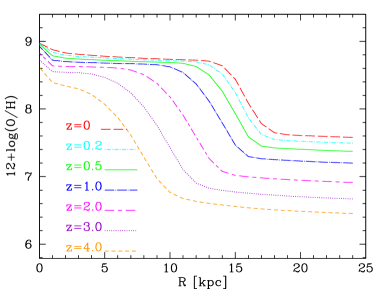
Figure 5: The radial distribution of the O abundances, $12+\log{({\rm O/H})}$, for different redshifts, as labelled. The results are for MOD1 and all radial regions.

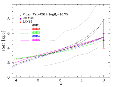
Figure 6: Evolution of the effective radius $R_{\rm eff}$ of models with the redshift $z$ compared with data from van der Wel et al. (2014) for galaxies with stellar mass $\log{M_{\star}}\sim 10.75$, shown as dashed lines with dots (the dotted lines are the curves $\pm\sigma$). The full purple dot represents the estimated effective radius for the MWG at the present time, while the red triangle is the averaged value measured for galaxies of the local Universe with GAMA data (Lange et al., 2015). Each model is represented with a different type of line and color as labelled.

In Fig. 5, the oxygen abundance, as $12+\log{({\rm O/H})}$, for MOD1 is represented as a function of the radius $R$ in kpc, for seven values of redshift: z= 0, 0.2, 0.5, 1.0, 2.0, 3.0 and 4.0. We have represented all computed radial regions. For higher redshifts the radial distributions are apparently very different than now, with a strong variation with redshift/time. However, we see that there is not a straight line with only one slope, but there is a clear line until a radius $R\sim 13-14$ kpc in $z=0$. Beyond this region there exists a strong downturn which would correspond to the edge of the stellar disc. This shape is similar to the one obtained by Wang et al. (2018, see their Fig.5) for the density of the Galactic disc. These authors study the radial density profile of the disc, confirming that it extends to 19 kpc, and separating the contributions of thin and thick disc for each radial bin. They find two breaks at R=11 kpc and R=14 kpc, thus dividing the radial distribution into three segments, one for $R<11$ kpc, other for $R$ in the range 16–19 kpc, and a middle transition zone between both. The scale lengths are 2.12 kpc in the inner region, 2.72 kpc in the outside, and 1.18 kpc in the intermediate one. The outer disc (starting at 14 kpc) is where the thick disc component becomes prominent. The thin disc, the dominant contributor to the inner region, begins to weaken at the first break, disappearing gradually within the transition region. These authors suggest that the stellar populations of the outer disc correspond to the thick disc and that the thin disc ends at a shorter radius. Our breaks, for the present time, occur at radii slightly higher, the first one at $\sim 14$ kpc, and the second at $\sim 17$ kpc. Considering the findings of Wang et al. (2018), the radial gradient for the disc must be measured with data from regions located within the first break, since the abundances of outer regions located at $R>16-17$ kpc would correspond, in our models, to the thick disc/halo regions, for which a flatter radial gradient is expected.

Apparently, the curves for other redshifts have the same behavior, with a smooth variation until a given radius and a decreasing after that. We should note that a variation of size with redshift is expected in the inside-out scenario of growth of discs. We need, therefore, to define a limiting or break radius –for each time– to estimate the radial gradient of the thin disc.

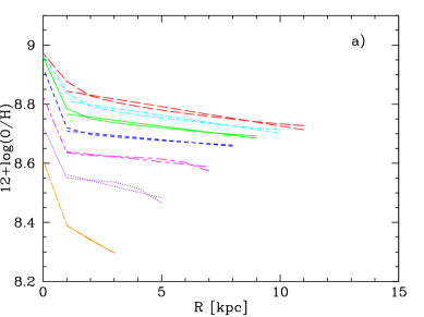
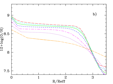
Figure 7: The oxygen abundances as $12+\log{({\rm O/H})}$ for MOD1 as a function of: a) the radius $R$, but only for regions located within the break of the radial distributions, $R_{\rm break}$. The least squares straight lines fitting the radial distributions are over-plotted in each redshift; b) the normalized radius $R/R_{\rm eff}$. Line coding is the same as in Fig. 5.

For each time step and model calculated, we have computed the effective radius in mass (or half mass radius), defined as the radius in which half of the total stellar mass of the disc (obtained simply by adding the stellar mass of each radial zone and time) is reached. The evolution with redshift of the effective radius, $R_{\rm eff}$, is shown in Fig. 6 for our 5 models. The final result, $R_{\rm eff}$(z=0) must be compared with the MWG data. From the binned observed radial distribution of stellar surface density for the MWG taken from MOL15, we obtain a $R_{\rm eff}=5.85$ kpc, which is in good agreement with the value 5.98 kpc given by de Vaucouleurs & Pence (1978). Moreover, we may find more estimates for this radius from the measured scale length of the Galactic disc. If we assume an exponential distribution for the stellar density:

$$\Sigma=\Sigma_{0}\,\exp{-R/R_{\rm D}},$$ (5)

the total mass of the stars in the disc is $M_{\rm D}=2\,\pi\,\Sigma_{0}\,R_{\rm D}^{2}$. Using this expression, the relationship of the effective radius with the scale length results:

$$R_{\rm eff}=1.678\,R_{\rm D}.$$ (6)

Table 4: Observational data for the effective radius $R_{\rm eff}$ of the MWG.

$R_{\rm eff}$	Reference
5.98	de Vaucouleurs & Pence (1978)
5.95	de Vaucouleurs (1983)
6.56	van der Kruit (1986)
4.49	Freudenreich (1996)
5.10	Gould, Bahcall, & Flynn (1996)
4.76	Zheng et al. (2001)
4.42	Jurić et al. (2008)
4.42	Siebert et al. (2008)
4.42	Sale et al. (2010)
6.46	Moni Bidin, Carraro, & Méndez (2012)
3.66	Bovy & Rix (2013)
4.61	Licquia, Newman, & Bershady (2016)
4.42	Bland-Hawthorn & Gerhard (2016)
4.17	McGaugh (2016)
5.95	Sofue (2018)

The photometric scale-length for MWG takes values between $R_{\rm D}=3.86$, and 2.64 kpc, depending on the technique, author or wavelength band. Therefore, in Fig. 6 we have used an averaged value, calculated from equation 6 and $R_{\rm D}$ from authors listed in Table LABEL:re, where we give this effective radius $R_{\rm eff}$, in column 1, as obtained from the scale-length $R_{\rm D}$ given by different authors, in column 2. From this method we have obtained an averaged value $<R_{\rm eff}>=5.07\pm 0.93$ kpc. This value is shown as a purple dot with error bars. We have also plotted the averaged observational point obtained with GAMA data by Lange et al. (2015) for local disc galaxies, shown as a red triangle at z=0 in the same Fig. 6, which is similar to the observational MWG averaged value. All our models end the evolution with a value compatible with the error bars of these observational estimates.

The effective radius of all our models follows a similar trend with redshift. We also included in the same Fig. 6 the evolution found by van der Wel et al. (2014) for galaxies with a similar stellar mass than MWG (column corresponding to $\log_{M_{*}}=10.75$ in their Table 2), shown as dashed lines with dots, and the respective $\pm\sigma$ limits, as dotted lines. In this figure we also included the fit given by these authors as a solid black line. Xiang et al. (2018), studying stellar populations of the local Universe with CALIFA data, also find that the scale-length $R_{\rm D}$ for the radial distribution of surface mass density yields a value of $\sim 4$ kpc for the young stellar populations and of $\sim 2$ kpc for the oldest ones. Bland-Hawthorn & Gerhard (2016) have already established that the scale length is smaller for the inner (old populations) regions than for the outer disc (young stellar populations). Taking into account the relationship of $R_{\rm D}$ with the effective radius, this implies that $R_{\rm eff}$ has also been smaller in the past than it is now.

Summarizing, $R_{\rm eff}$ is smaller at $z=4$ than now and the evolution of the modeled radius is in agreement with observational estimations. Since the disc is short for higher redshifts, a smaller radial range should be used to estimate the radial gradient of abundances at other redshifts/times.

If we assume a Freeman law for disc, the optical radius, defined as $R_{\rm opt}=R_{25}$ (the isophote of 25 mag/arcsec² or equivalently the radius enclosing the 83% of the light) is $R_{\rm opt}\sim 3.2\,R_{\rm D}$, and, using the above relationship between $R_{\rm D}$ and $R_{\rm eff}$, $R_{\rm opt}\sim$1.9 – 2.0$\,R_{\rm eff}$, using for both $R_{\rm D}$ and $R_{\rm eff}$ the light profile, (slightly different if the mass density profile is used instead). As demonstrated by Sánchez et al. (2014), all galaxies show a similar behaviour in the radial distribution of oxygen abundances out to 2–2.5 R_eff. Thus, by assuming an effective radius for MWG of $\sim 5.07\pm 0.93$ kpc, the radial regions where an uniform radial gradient may be obtained will be within 10.14–12.675  kpc. Taking into account the uncertainties in the effective radius, we define an arbitrary break radius as $R_{\rm break}=\sim 2.6\,R_{\rm eff}$, (which gives 13.18 kpc for the present time). So, our criteria for including only the disc component in the calculation of the gradient is choosing regions located at $R<R_{\rm break}=2.6\,R_{\rm eff}$, which is in good agreement with Sánchez et al. (2014). An exact value of this break radius, (2.6, 2.2 or even 2 times the effective radius) can not be given, since the relationship between the optical radius (from the luminosity distribution) and the half mass radius (from the mass distribution) is not actually very well established. The only important thing here is that the same ratio $\rm R_{break}/R_{eff}$ must be used along the time, thus taking the growth of the disk into account for the computation of the radial gradient. This way the break radius will be $\leq 4$ kpc at $z=4$ (just where the radial distribution begins to be steeper, see the orange line in Fig. 5) and not 14-15 kpc as occurs in the present time distribution. Therefore, it is important to define in each time the radial range over which we can accurately measure the value of the radial gradient in order to estimate its correct evolution.

In Fig. 7 we show in panel a) a plot similar to Fig. 5, but now using only regions before the break of the abundance distributions, that is within $R_{\rm break}=2.6\,R_{\rm eff}$. These lines will appear slightly steeper for $z=4$ than now, flattened for $z=3$ and $z=1$, and steepens slightly again for $z=0.5$ until $z=0$. Also, we shown in this Fig. 7 the least squares straight lines obtained for the disc (eliminating the central bulge, $R=0\,{\rm kpc}$ in the calculation, in order to compute the disk radial gradient) which are over-plotted in each redshift. The resulting radial gradients are given in Table 5, column 3. The radial gradient is not exactly the same at all times, but, following this approach, the evolution is much smoother than the one from our previous calculations using the whole radial range.

Table 5: Radial gradients of oxygen abundances obtained from MOD1 for different redshifts.

Time	z	$\nabla_{O/H}$
[Gyr]		[dex kpc-1]	[dex R${}_{\rm eff}^{-1}$]
13.20	0.0	$-0.0131\pm 0.0012$	$-0.073\pm 0.007$
10.70	0.2	$-0.0116\pm 0.0010$	$-0.061\pm 0.005$
8.00	0.5	$-0.0106\pm 0.0010$	$-0.053\pm 0.005$
5.50	1.0	$-0.0125\pm 0.0025$	$-0.056\pm 0.011$
2.70	2.0	$-0.0251\pm 0.0067$	$-0.092\pm 0.025$
1.50	3.0	$-0.0476\pm 0.0108$	$-0.133\pm 0.030$
0.90	4.0	$-0.0568\pm 0.0062$	$-0.098\pm 0.011$

For $z=4$ the radial gradient is more similar to the one for $z=0$, now when it is measured out to $R\sim$ 3–5 kpc instead of, say, out to 15 kpc as in the case for redshift $z$=0. To measure the radial gradient of abundance using a radial range up 14 kpc when the optical disk has a size not larger than 5 kpc seems quite unreasonable. To limit the radial range allows a certain and uniform estimate of the radial gradient of the disk and its correct evolution.

Our conclusion is, therefore, that for our models the radial gradient does not change appreciably with redshift if we measure it within the thin disc (whose size obviously decreases with increasing redshift). More specifically, within a break radius $R_{\rm break}=2.6\times R_{\rm eff}$, it flattens from $z=4$ until $z=1$ and steepens again, although slightly, from $z=1$ until now. In Fig. 7, panel b) we show the same results as in panel a), but now as a function of the normalized radius $R/R_{\rm eff}$. We see a clear radial gradient until $R/R_{\rm eff}\sim$ 2.3–2.6. Measuring the radial gradient by fitting least squares straight lines for $R/R_{\rm eff}<2.6$, we obtain the values given in column 4 of the Table 5. We see again that the gradient did not change appreciably since $z=1.0$.

4.2 Comparison of models

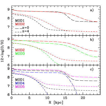
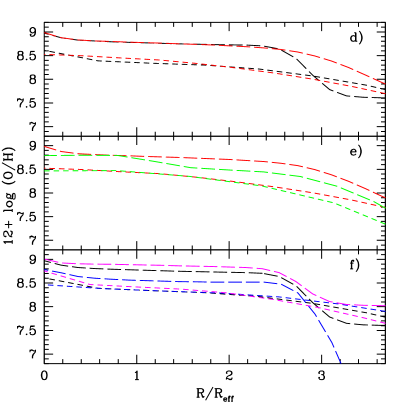
Figure 8: The radial distribution of O abundances, $12+\log{({\rm O/H})}$, as a function of the radius $R$ in kpc in the left panels, while in right panels we show the same models as a function of $R/R_{\rm eff}$. Two/three models are shown in each panel: a) and d) MOD 1 and MOD 2, b) and e) MOD2 and MOD3, and c) and f) MOD1, MOD4 and MOD5. Line colors have the same meaning as in Fig. 6. Results for redshifts $z=0$ and $z=4$ are shown as long-dashed and short-dashed lines, respectively.

In this subsection we compare MOD1 with the other models listed in Table LABEL:models. In the left panels of Fig. 8 the comparison is done using $R$, while in the right panels abundances are represented as $R/R_{\rm eff}$. In the first row of Fig. 8—panels a) and d)—we compare MOD1 and MOD2, where the infall rate is the same, but the formation of molecular clouds is done with different prescriptions, as described in Mollá et al. (2017). We see that they are clearly different for the outer regions of the disc, with a smoother radial gradient for MOD2 as compared with MOD1. The last one shows a strong decrease in the outer disc and then a very flat radial distribution, in a similar way to the density profile (Wang et al., 2018), while MOD2 does not present this strong break, but a continuously decreasing function. We should note that the effective radius evolves in a different way in both models, as shown in Fig. 6. Both features balance each other, so that if we see the distributions as a function of the effective radius, we find a similar evolution in both cases. Except in the very outer disc, where differences among models arise, mainly at $z=0$.

We compare in the second row of Fig. 8 two models using the same prescription to form molecular clouds, but different infall rates: MOD2, which uses the new infall rates calculated in MOL16, and MOD3, which uses the infall rates as in MD05. In fact, both models also differ in the combination IMF+stellar yields. However, as we demonstrated in MOL15, all combinations give similar radial gradient and only absolute abundances are changed by these ingredients. MOD3 has a stronger variation of infall rates with radius than MOD2 and, consequently, shows a slightly steeper radial gradient of abundances. Again, however, we find smaller differences when we compare distributions as a function of $R/R_{\rm eff}$, mainly at $z=4$.

Another debated question is if the radial gradient maintains the same slope for all observed radial range or if it flattens (or steepens) in the outer disc. The radial gradient in MWG might be compatible with a same slope across the disc until $R\leq 18$ kpc (Fernández-Martín et al., 2017; Esteban et al., 2017). However, for the CALIFA and MUSE surveys, some authors (Sánchez et al., 2014; Sánchez-Menguiano et al., 2016, 2018) find a flattening beyond $R>2--2.5\,R_{\rm eff}$. We also find a plateau with $12+\log{({\rm O/H})}\sim 7.5$ dex for $z=0$ in MOD1 (see Fig. 5). In our scenario there is also star formation in the halo, with an efficiency $\epsilon_{h}=0.01--0.03$, as chosen in Ferrini et al. (1992) to reproduce the star formation history and age-metallicity relation in the Galactic halo, and used in MOD1, MOD2 and MOD3. This implies that the gas infalling in the disc is not primordial but it is pre-enriched, contributing to the level of metal abundances in the disc. Its effect is not very apparent in the bright regions of the disc, with much higher abundances than the ones of the infalling gas, but it may be seen clearly in the outer regions, where the star formation rates are very low and, consequently, the infall may enrich the ISM of these regions. In order to check if this possibility may produce a flattening of the oxygen abundances in the outer disc, we have now calculated another two models, both similar to MOD1 but modifying the star formation efficiency of the halo to be $\epsilon_{h}=0.00$ (primordial abundances for the infalling gas) and $\epsilon_{h}=0.10$ in MOD4 and MOD5, respectively, in order to check if the outer regions of the disc are modified as consequence of the different infall enrichment.

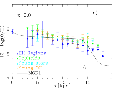
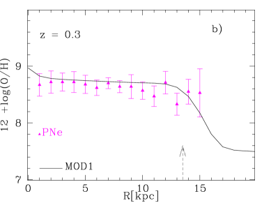
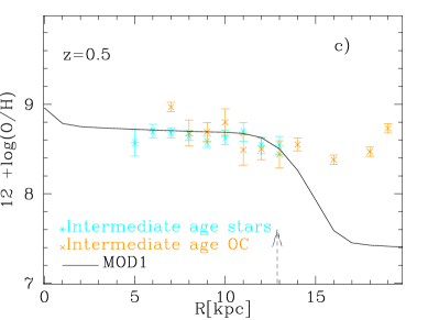
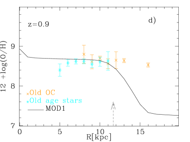
Figure 9: The oxygen abundances as a function of the galactocentric radius $R$. Panels show the comparison of MOD1: a) at the present time ($z=0$) with data from Hii regions, Cepheid stars, young stars and young OC, as blue circles, green squares, cyan stars and orange crosses, respectively; b) at $z=0.3$ and PNe data as magenta triangles; c) at $z=0.5$ with intermediate age stars and OC, as cyan stars and orange crosses, respectively; d) at $z=0.9$ with data from old OC and old stars, as orange crosses and cyan stars, respectively. In each panel an arrow indicates the size of the expected break, $R_{\rm break}\rm\sim 2.60\times\rm R_{eff}$. All points are the binned results obtained as explained in Section  2.

We see in panel c) of Fig. 8 that the oxygen abundance for $z=0$ in the external disc drops continuously in MOD4, while it takes a constant value of $\sim 8.0$ dex for MOD5. This value is $\sim 0.5$ dex higher than in MOD1, where this outer abundance is $\sim 7.5$ dex. Therefore, a flattening of the gradient in the outer discs, with a value of $12+\log({\rm O/H})\sim 8.0$ dex as observed by CALIFA and MUSE, is in agreement with this possibility of star formation in the halo, and the subsequent metal enriched infall. This hypothesis of an enriched infall as the cause of the flat radial distributions of abundances in the outer disc was also proposed by other authors, as Bresolin et al. (2012, 2016). This abundance will be similar for all galaxies when a same efficiency for the star formation in the halo is used. A different plateau for each galaxy would be also reasonable if the halo has a different evolution in each case, depending on the environment or on the interactions suffered by the proto-halo in a early phase of the evolution. We should note that in the literature there are other interpretations for these flattening of the gradient at the outer disc as, e.g., a star formation efficiency that is roughly constant for $R>R_{\rm eff}$ (see Kudritzki et al., 2015, for details).

In any case, when we represent these distributions as a function of a normalized radius (right panels of Fig.8), we found that all of models show a very similar radial gradient, with only small differences among them. This has previously been shown for a suite of simulated disc galaxies in Few et al. (2012), where while the metallicity gradients with normalized radius have a wider spread than seen here, no trends are found with mass or environment (in a limited sense) as are found in absolute gradient (this analysis is expanded in Pilkington et al., 2012). We find here that the star formation, the infall rate or the stellar yields do not modify the basic value of gradient. This gradient shows a very similar slope for all redshifts, particularly if we use only the disc regions, without the central region at $R=0$, where we represent the bulge.

5 Discussion: Evolution of the radial gradient

5.1 Evolution of the gradient with time

In the time range $3\leq t\leq 13.2$ Gyr, the possible evolution of the gradient seems to be rather undetectable. Thus, a clear separation in data coming from H ii regions and PNe of 2–4 Gyr old will not be apparent, such as SH10, MAC13, and M16 claim. We see this clearly in Fig. 9, where O abundances of MOD1 are compared in: a) for $z=0$ with our binned data from Hii regions, Cepheid stars, young stars and young OC; in panel b) for $z=0.3$ with PNe data; in panel c) for $z=0.5$ with intermediate age stars and OC data; and in panel d) for $z=0.9$ with old age stars and OC.

The model results agree with the generic trend of observational data in all panels of Fig. 9, although there are dots corresponding to OC data slightly above the line in panels c) and d) for the outer regions represented. This result may be related to previous arguments given in Subsection 3.1: in the outer regions, data would not correspond to the thin disc component, but to the thick disc or the halo populations. For $z=0$ the optical radius for the MWG is around 11 kpc and the drop begins at $R=14$ kpc. For $z=0.9$, following our models, it would be $R_{\rm opt}\sim 9$ kpc, and the first break would be at $R\sim 11$ kpc, as shown in MOD1. It is, therefore, possible that last points after $R_{\rm break}$ pertain to the transition region thin-thick disc, before to reach the real outer region for which a flatter radial gradient is expected. There are some studies (Nordström et al., 2004; Allende Prieto et al., 2006; Cheng et al., 2012; Carrell, Chen, & Zhao, 2012; Boeche et al., 2014) using data from the thick disc which also found flat or even positive radial gradient for the largest galactocentric distances. These data in the outer regions may also be the consequence of a stellar radial migration process, meaning that old objects are located further from their birth radius.

The time evolution of the gradient is shown in Fig. 10. In this figure, we represent the corresponding radial gradient obtained in Table 2, in the times associated, following the assumed age, to each objects: Hii regions and Cepheids at $t=13.2$ Gyr; Young stars and OC between $t=11$ and the present time; PNe between 9 and 11 Gyr; intermediate age stars and OC between 5 and 11 Gyr; and old stars and OC between 0 and 5 Gyr. Over them, we plot the gradients obtained by our 5 models. When the gradients are measured within the corresponding disc for each time, most of them do not give a strong evolution in time for the O radial gradient as it is shown, mainly for MOD1, MOD2 and MOD5; indeed they are around $-0.02$ or $-0.03$ dex kpc^-1 from $t=4$ Gyr until now. MOD3 (with the old prescription of infall of gas from MD05) clearly does not fit this evolution shown by data, while MOD4 show a very strong flattening from $t=1$ Gyr until $t=2$ Gyr, and a continuous steepening since then until now.

If we accept this behavior of our models, the radial gradient of O abundances do not evolve very much with time in the last 10 Gyr. The observational data presented in Fig. 10 also supports this conclusion. Following these data the radial gradient has been basically the same for times from 4-5 Gyr until 13 Gyr, only showing a steepening in the last times. Only the flat radial distribution for the oldest stars is out of this trend, showing a large difference with the point of the oldest OC, (although it is necessary to take into account that the radial range of the old stars is very narrow compared with the one in which other object abundances have been measured). As we demonstrate above, finding this smooth behavior for the slope, basically without or with a mild evolution, is mainly the consequence of restricting the radial range in our models to the break radii, which is around $R_{\rm break}=2.6\times R_{\rm eff}$. In the case of the observational data, this result implies that objects beyond this limit might be members of the thick disc or the halo. Other possibility is that some stars or OC have migrated to the outer disc. This would be more likely for the old objects, which would explain the points above the line of the model in Fig.9c and Fig.9d. It would imply that these objects do not represented the abundances of the gas of the regions were are located, but the ones of the regions were they were created. Curiously, this seems to occur more for old OC than for old stars.

Our conclusion is that, in any case, it is necessary to take into account that the disc grows with time, and that at the time when objects with old/intermediate ages were created, the disc was smaller than now (see Section 3). Therefore, if we want to measure with good accuracy the evolution of the radial gradient of abundances in the thin disc, we need to determine very carefully which component are we observing and the radial range where to measure it.

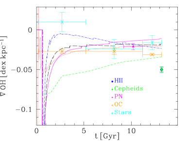
Figure 10: Evolution of the O radial gradient along time for different objects. The predictions of models are shown with the same coding of lines than in Fig.6.

5.2 Evolution of the gradient with redshift

In other works related with the evolution of the radial gradient of metallicity, data or model results are shown as a function of redshift. For that reason, in order to compare the predictions of our models with other results in the literature, we shown here the predictions for earlier times as a function of the redshift, instead of time. We show in Fig. 11 the evolution of the gradient, $\nabla_{OH}$, along redshift for our models. In panel a) the results are compared with previous chemical evolution models (Mollá, Ferrini, & Díaz, 1997, and MD05 –here MOD3) and cosmological simulations from Pilkington et al. (2012); Gibson et al. (2013); Tissera et al. (2017) as labelled. Pilkington et al. (2012) gave results similar to MD05 and Mollá, Ferrini, & Díaz (1997) using all radial regions. The recent results from Tissera et al. (2017) are closer to MD05 (MOD3) computed for regions within the optical disc, while MOD1, MOD2 and MOD5 give a behavior more similar to Gibson et al. (2013), with a smooth evolution almost nonexistent for some of them. MOD4 (without SFR in the halo) show a clear flattening until $z=1$ and then a steepening in the last times, while in MOD3 the gradient is continuously flattening as MOD5 also does. MOD1 and MOD2 have a similar shape as MOD4 but smoother than this one.

In panel b) of Fig.11 we compare our results with the same data as in Fig. 10. Although our models show a smooth behavior for the gradient in agreement with these observational results, we see that the gradient was steeper at higher redshifts ($z>2$ or 3). This is important because it is related to the phase of the disc formation. At a time of $t=1\,{\rm or}\,2$ Gyr, when there is sufficient gas in the centre of the future disc, star formation begins and the first elements appears in the ISM. This is the way in which we achieve higher abundances in the central regions while the surroundings remain almost primordial, resulting in a strong radial gradient of abundances. These first phases are numerical unstable (as it is seen in Fig. 10), making it more difficult to measure the gradient. In fact, real galaxies also will have unstable phases and this fact must be taken into account when observations will be performed over discs probably in the formation process.

In panel c), we represent $\nabla_{OH}$ vs. the normalized radius ${R/R_{\rm eff}}$. MOD1, MOD2, even MOD5, are within the evolution obtained by Tissera et al. (2017), albeit in the shallower frontier. Our resulting gradient is in very good agreement with the universal value from Sánchez et al. (2014); Sánchez-Menguiano et al. (2016, 2018) at $z=0$ for all models. In this case the evolution seems stronger than in previous panels, due to the evolution of the effective radius. Now differences between models are larger: MOD3 and MOD5 show a continuous flattening, MOD2 is basically flat and MOD1 and MOD4 show a flattening until $z\sim 1$ with a steepening at the end.

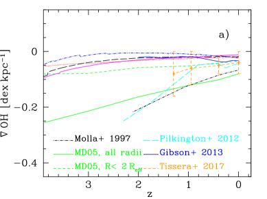
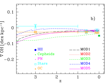
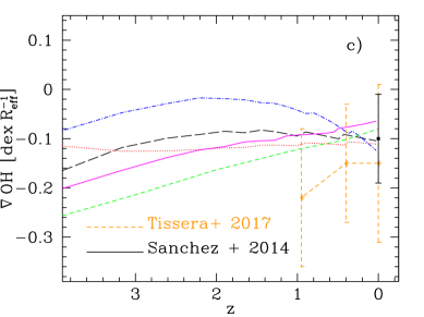
Figure 11: The evolution with redshift of the radial gradient of O abundances: a) in dex kpc^-1 units compared with cosmological simulations from Gibson et al. (2013) and Tissera et al. (2017), as labelled; b) compared with observational data from different objects compiled in this work, as labelled; c) in dex$\,R_{\rm eff}^{-1}$ units compared with cosmological simulations from Tissera et al. (2017) and data from Sánchez et al. (2014); Sánchez-Menguiano et al. (2016) for the present time. All panels show models MOD1 to MOD5 with the same line coding as labelled in panel b).

6 CONCLUSIONS

In this work we have highlighted the importance of determining the radial gradient of O abundances in the disc of the Milky Way Galaxy. We summarize the most important results obtained in this work.

1. It is essential to determine the disc radial gradient always within the optical radius or a radius slightly higher, (we use a maximum value $R_{\rm break}\leq 2.6\,R_{\rm eff}=1.3\,R_{\rm opt}$ for calculating it). We claim that the use of a variable radial range, which takes into account the growth of the disk along the time or redshift, is an important caveat for estimating the correct evolution of the disk radial gradient.

2. We built five models to analyse the time evolution of the O radial gradient. The influence of the infall of gas was examined in model MOD3, which uses an infall prescription from Mollá & Díaz (2005). The others four models use the new prescription from Mollá et al. (2016) which give smoother infall of gas. We also tested the influence of the prescriptions of Hi to H₂ conversion process through comparison of models MOD1 (prescription named ASC in Mollá et al., 2017) and MOD2 (prescription named STD in Mollá et al., 2017). We tested the hypothesis of having an enriched infall from the halo, by using different star formation efficiency in the halo, a higher efficiency in MOD5 than in the other models and the hypothesis of no star formation in the halo (primordial abundances for the infalling gas) in MOD4.

3. The evolution of the gradient measured within the thin disc until a $R_{\rm break}$ variable with time is mild for MWG, with an average value $\nabla_{\rm OH}\sim-0.02\,{\rm or}\,-0.03\rm\,dex\,kpc^{-1}$ with slight differences among models.

4. When it is measured as a function of normalized radius, we obtain a value $\nabla_{OH}\sim-0.10\,{\rm dex}\,R_{\rm eff}^{-1}$ for $0<z<1.5$ in models MOD1, MOD2 and MOD4 with our new infall prescription from Mollá et al. (2016), which is in excellent agreement with the local universal gradient found by Sánchez et al. (2014); Sánchez-Menguiano et al. (2016, 2017) for CALIFA and MUSE surveys galaxies. Taking into account that we calibrate our model to reproduce the radial distributions of the disc (gas, stars, SFR and elemental abundances), but not the effective radius, nor the normalized gradient, we consider this fit a success of our model. The gradient is slightly flatter for models MOD3 (infall type from Mollá & Díaz (2005)) and MOD5 (lower star formation efficiency in the halo). MOD4 (no star formation in the halo) shows an early flattening and then a steepening, reaching in the end the same present day value as observed.

5. The oxygen abundance for $z=0$ in the outer regions drops continuously in MOD4, while it takes a constant value of $\sim 8.0$ dex for MOD5. This value is $\sim 0.5$ dex higher than in MOD1, where this outer abundance is $\sim 7.5$ dex. Therefore, a flattening of the gradient in the outer discs, with a value of $12+\log({\rm O/H})\sim 8.0$ dex as observed by CALIFA and MUSE, is in agreement with the possibility of star formation in the halo, and the subsequent metal enriched infall.

6. The radial gradient of abundance in isolated galaxies is a scale effect which depends on disc growth. When measured within the optical disc, it maintains a similar value as it evolves where this occurs quietly i.e., without interactions with the environment and once the disc is formed, at least until $z=1.5$. For higher redshifts, our models have different evolutions, depending on the hypothesis used for the infall rate, to form molecular clouds, or to form stars in the halo. The stronger radial gradient appears in the early phase of the disc formation, defined by the dynamical mass of each galaxy. This point will be analysed in more detail in the next future, when models for other type/mass of galaxies and the corresponding radial gradients will be presented.

These conclusions highlight the needed for further investigation in order to clarify the differences between theoretical models, as well as to extract out and interpret observations at intermediate and high redshifts. We will address in a forthcoming paper the possible variations of these results for other spiral galaxies, analyzing the dependence on the stellar mass and size (Mollá et al. in preparation).

References

- Allende Prieto et al. (2006) Allende Prieto C., Beers T. C., Wilhelm R., Newberg H. J., Rockosi C. M., Yanny B., Lee Y. S., 2006, ApJ, 636, 804
- Anders et al. (2017) Anders F., et al., 2017, A&A, 600, A70
- Andreuzzi et al. (2011) Andreuzzi G., Bragaglia A., Tosi M., Marconi G., 2011, MNRAS, 412, 1265
- Andrievsky et al. (2016) Andrievsky S. M., Martin R. P., Kovtyukh V. V., Korotin S. A., Lépine J. R. D., 2016, MNRAS, 461, 4256
- Ascasibar et al. (2018) Ascasibar,Y., et al. 2018, in preparation
- Asplund et al. (2009) Asplund M., Grevesse N., Sauval A. J., Scott P., 2009, ARA&A, 47, 481
- Balser et al. (2011) Balser D. S., Rood R. T., Bania T. M., Anderson L. D., 2011, ApJ, 738, 27
- Bastian & Lardo (2017) Bastian, N., & Lardo, C., 2017, arXiv:1712.01286
- Bergemann et al. (2014) Bergemann M., et al., 2014, A&A, 565, A89
- Bland-Hawthorn & Gerhard (2016) Bland-Hawthorn J., Gerhard O., 2016, ARA&A, 54, 529
- Bovy et al. (2012) Bovy J., Rix H.-W., Liu C., Hogg D. W., Beers T. C., Lee Y. S., 2012, ApJ, 753, 148
- Bovy & Rix (2013) Bovy J., Rix H.-W., 2013, ApJ, 779, 115
- Boeche et al. (2014) Boeche C., et al., 2014, A&A, 568, A71
- Bresolin et al. (2012) Bresolin, F., Kennicutt, R. C., & Ryan-Weber, E. 2012, ApJ, 750, 122
- Bresolin et al. (2016) Bresolin, F., Kudritzki, R.-P., Urbaneja, M. A., et al. 2016, ApJ, 830, 64
- Cantat-Gaudin et al. (2016) Cantat-Gaudin T., Donati P., Vallenari A., Sordo R., Bragaglia A., Magrini L., 2016, A&A, 588, A120
- Casagrande et al. (2011) Casagrande L., Schönrich R., Asplund M., Cassisi S., Ramírez I., Meléndez J., Bensby T., Feltzing S., 2011, A&A, 530, A138
- Carrell, Chen, & Zhao (2012) Carrell K., Chen Y., Zhao G., 2012, AJ, 144, 185
- Carrera & Pancino (2011) Carrera R., Pancino E., 2011, A&A, 535, A30
- Cavichia, Costa, & Maciel (2011) Cavichia O., Costa R. D. D., Maciel W. J., 2011, RMxAA, 47, 49
- Cavichia et al. (2014) Cavichia O., Mollá M., Costa R. D. D., Maciel W. J., 2014, MNRAS, 437, 3688
- Chen, Hou, & Wang (2003) Chen L., Hou J. L., Wang J. J., 2003, AJ, 125, 1397
- Cheng et al. (2012) Cheng J. Y., et al., 2012, ApJ, 746, 149
- Chiappini, Matteucci, & Gratton (1997) Chiappini C., Matteucci F., Gratton R., 1997, ApJ, 477, 765
- Chieffi & Limongi (2004) Chieffi A., Limongi M., 2004, ApJ, 608, 405 (CLI)
- Cunha et al. (2016) Cunha K., et al., 2016, AN, 337, 922
- Daniel & Wyse (2018) Daniel K. J., Wyse R. F. G., 2018, MNRAS, 476, 1561
- Diaz & Tosi (1984) Diaz A. I., Tosi M., 1984, MNRAS, 208, 365
- Di Matteo et al. (2013) Di Matteo P., Haywood M., Combes F., Semelin B., Snaith O. N., 2013, A&A, 553, A102
- Edvardsson et al. (1993) Edvardsson B., Andersen J., Gustafsson B., Lambert D. L., Nissen P. E., Tomkin J., 1993, A&AS, 102, 603
- Esteban et al. (2013) Esteban C., Carigi L., Copetti M. V. F., García-Rojas J., Mesa-Delgado A., Castañeda H. O., Péquignot D., 2013, MNRAS, 433, 382
- Esteban et al. (2017) Esteban C., Fang X., García-Rojas J., Toribio San Cipriano L., 2017, MNRAS, 471, 987