The Bregman chord divergence

Abstract

Distances are fundamental primitives whose choice significantly impacts the performances of algorithms in machine learning and signal processing. However selecting the most appropriate distance for a given task is an endeavor. Instead of testing one by one the entries of an ever-expanding dictionary of ad hoc distances, one rather prefers to consider parametric classes of distances that are exhaustively characterized by axioms derived from first principles. Bregman divergences are such a class. However fine-tuning a Bregman divergence is delicate since it requires to smoothly adjust a functional generator. In this work, we propose an extension of Bregman divergences called the Bregman chord divergences. This new class of distances does not require gradient calculations, uses two scalar parameters that can be easily tailored in applications, and generalizes asymptotically Bregman divergences.

Keywords: Bregman divergence, Jensen divergence, skewed divergence, clustering, information fusion.

1 Introduction

Dissimilarities (or distances) are at the heart of many signal processing tasks [13, 6], and the performance of algorithms solving those tasks heavily depends on the chosen distances. A dissimilarity $D(O_{1}:O_{2})$ between two objects $O_{1}$ and $O_{2}$ belonging to a space $\mathcal{O}$ (e.g., vectors, matrices, probability densities, random variables, etc.) is a function $D:\mathcal{O}\times\mathcal{O}\rightarrow[0,+\infty]$ such that $D(O_{1}:O_{2})\geq 0$ with equality if and only if $O_{1}=O_{2}$. Since a dissimilarity may not be symmetric (i.e., an oriented dissimilarity with $D(O_{1}:O_{2})\not=D(O_{2}:O_{1})$), we emphasize this fact using the notation ’:’. The reverse dissimilarity or dual dissimilarity is defined by

$$D^{*}(O_{1}:O_{2}):=D(O_{2}:O_{1}),$$ (1)

and satisfies the involutive property: $({D^{*}})^{*}=D$. When a symmetric dissimilarity further satisfies the triangular inequality

$$D(O_{1},O_{2})+D(O_{2},O_{3})\geq D(O_{1},O_{3}),\quad\forall O_{1},O_{2},O_{3}\in\mathcal{O},$$ (2)

it is called a metric distance.

Historically, many ad hoc distances have been proposed and empirically benchmarked on different tasks in order to improve the state-of-the-art performances. However, getting the most appropriate distance for a given task is often an endeavour. Thus principled classes of distances have been proposed and studied. Among those generic classes of distances, three main types have emerged:

• The Bregman divergences [7, 5] defined for a strictly convex and differentiable generator $F\in\mathcal{B}:\Theta\rightarrow\mathbb{R}$:

  $$B_{F}(\theta_{1}:\theta_{2}):=F(\theta_{1})-F(\theta_{2})-(\theta_{1}-\theta_{2})^{\top}\nabla F(\theta_{2}),$$ (3)

  measure the dissimilarity between parameters $\theta_{1},\theta_{2}\in\Theta$. We use the term “divergence” (rooted in information geometry [3]) instead of distance to emphasize the smoothness property of the distance. The dual Bregman divergence $B_{F}^{*}(\theta_{1}:\theta_{2})$ is obtained from the Bregman divergence induced by the Legendre convex conjugate:

  $$B_{F}^{*}(\theta_{1}:\theta_{2}):=B_{F}(\theta_{2}:\theta_{1})=B_{F^{*}}(\nabla F(\theta_{1}):\nabla F(\theta_{2})),$$ (4)

  where the Legendre-Fenchel transformation is defined by:

  $$F^{*}(\eta)=\sup_{\theta\in\Theta}\{\theta^{\top}\eta-F(\theta)\}.$$ (5)

• The Csiszár $f$-divergences [1, 11] defined for a convex generator $f\in\mathcal{C}$ satisfying $f(1)=0$:

  $$I_{f}[p_{1}:p_{2}]:=\int_{\mathcal{X}}p_{1}(x)f\left(\frac{p_{2}(x)}{p_{1}(x)}\right)\mathrm{d}\mu(x),$$ (6)

  measure the dissimilarity between probability densities $p$ and $q$ that are absolutely continuous with respect to a base measure $\mu$ (defined on a support $\mathcal{X}$). A scalar divergence is a divergence acting on scalar parameters, i. e., a 1D divergence. A separable divergence is a divergence that can be written as a sum of elementary scalar divergences. The $f$-divergences are separable divergences since we have:

  $$I_{f}[p:q]=\int i_{f}[p(x):q(x)]\mathrm{d}\mu(x),$$ (7)

  with the scalar $f$-divergence $i_{f}[a:b]:=af\left(\frac{b}{a}\right)$.

  The dual $f$-divergence is obtained for the generator $f^{\diamond}(u):=uf(1/u)$ (diamond $f$-generator) as follows:

  $$I_{f}^{*}[p:q]:=I_{f}[q:p]=I_{f^{\diamond}}[p:q].$$ (8)

  We may $J$-symmetrize a $f$-divergence by defining its generator $f^{\circ}$:

  $$J_{f}[p:q] = \frac{1}{2}(I_{f}[p:q]+I_{f}[q:p]),$$ (9)

  $$= I_{f^{\circ}}[p,q],$$ (10)

  with

  $$f^{\circ}(u):=\frac{1}{2}\left(f(u)+f^{*}(u)\right).$$

  Alternatively, we may JS-symmetrize the $f$-divergence by using the following generator $f^{\bullet}$:

  $$\mathrm{JS}_{f}[p:q] := \frac{1}{2}\left(I_{f}\left[p:\frac{p+q}{2}\right]+I_{f}\left[q:\frac{p+q}{2}\right]\right),$$ (11)

  $$= I_{f^{\bullet}}[p,q],$$ (12)

  $$f^{\bullet}(u) := \frac{1+u}{4}\left(f\left(\frac{2u}{1+u}\right)+f\left(\frac{2}{1+u}\right)\right).$$ (13)

• The Burbea-Rao divergences [8] also called Jensen divergences because they rely on the Jensen’s inequality [15] for a strictly convex function $F\in\mathcal{J}:\Theta\rightarrow\mathbb{R}$:

  $$J_{F}(\theta_{1},\theta_{2}):=\frac{F(\theta_{1})+F(\theta_{2})}{2}-F\left(\frac{\theta_{1}+\theta_{2}}{2}\right)\geq 0.$$ (14)

  We note in passing that Bregman divergences can be extended to strictly convex and non-differentiable generator as well [18, 27].

These three fundamental classes of distances are not mutually exclusive, and their pairwise intersections (e.g., $\mathcal{B}\cap\mathcal{C}$ or $\mathcal{J}\cap\mathcal{C}$) have been studied in [26, 2, 16]. The ’:’ notation between arguments of distances emphasizes the potential asymmetry of distances (oriented distances with $D(\theta_{1}:\theta_{2})\not=D(\theta_{2}:\theta_{1})$), and the brackets surrounding distance arguments indicate that it is a statistical distance between probability densities, and not a distance between parameters. Using these notations, we express the Kullback-Leibler distance [10] (KL) as:

$$\mathrm{KL}[p_{1}:p_{2}]:=\int p_{1}(x)\log\frac{p_{1}(x)}{p_{2}(x)}\mathrm{d}\mu(x).$$ (15)

The KL distance between two members $p_{\theta_{1}}$ and $p_{\theta_{2}}$ of a parametric family $\mathcal{F}$ of distributions amount to a parameter divergence:

$$\mathrm{KL}_{\mathcal{F}}(\theta_{1}:\theta_{2}):=\mathrm{KL}[p_{\theta_{1}}:p_{\theta_{2}}].$$ (16)

For example, the KL statistical distance between two probability densities belonging to the same exponential family or the same mixture family amounts to a (parameter) Bregman divergence [3, 25]. When $p_{1}$ and $p_{2}$ are finite discrete distributions of the $d$-dimensional probability simplex $\Delta_{d}$, we have $\mathrm{KL}_{\Delta_{d}}(p_{1}:p_{2})=\mathrm{KL}[p_{1}:p_{2}]$. This explains why sometimes we can handle loosely distances between discrete distributions as both a parameter distance and a statistical distance. For example, the KL distance between two discrete distributions is a Bregman divergence $B_{F_{\mathrm{KL}}}$ for $F_{\mathrm{KL}}(x)=\sum_{i=1}^{d}x_{i}\log x_{i}$ (Shannon negentropy) for $x\in\Theta=\Delta_{d}$. Extending $\Theta=\Delta_{d}$ to positive measures $\Theta=\mathbb{R}_{+}^{d}$, this Bregman divergence $B_{F_{\mathrm{KL}}}$ yields the extended KL distance: $\mathrm{eKL}[p:q]=\sum_{i=1}^{d}p_{i}\log\frac{p_{i}}{q_{i}}+q_{i}-p_{i}$.

Whenever using a functionally parameterized distance in applications, we need to choose the most appropriate functional generator, ideally from first principles [12, 4, 3]. For example, Non-negative Matrix Factorization (NMF) for audio source separation or music transcription from the signal power spectrogram can be done by selecting the Itakura-Saito divergence [14] (a Bregman divergence for the Burg negentropy $F_{\mathrm{IS}}(x)=-\sum_{i}\log x_{i}$) that satisfies the requirement of being scale invariant: $B_{F_{\mathrm{IS}}}(\lambda\theta:\lambda\theta^{\prime})=B_{F_{\mathrm{IS}}}(\theta:\theta^{\prime})=\sum_{i}\frac{\theta_{i}}{\theta_{i}^{\prime}}-\log\frac{\theta_{i}}{\theta_{i}^{\prime}}-1$ for any $\lambda>0$. When no such first principles can be easily stated for a task [12], we are left by choosing manually or by cross-validation a generator. Notice that the convex combinations of Csiszár generators is a Csiszár generator (idem for Bregman divergences): $\sum_{i}\lambda_{i}I_{f_{i}}=I_{\sum_{i}\lambda_{i}f_{i}}$ for $\lambda$ belonging to the standard simplex $\Delta_{d}$. Thus in practice, we could choose a base of generators and learn the best distance weighting (by analogy to feature weighting [20]). However, in doing so, we are left with the problem of choosing the base generators, and moreover we need to sum up different distances: This raises the problem of properly adding distance units! Thus in applications, it is often preferable to consider a smooth family of generators parameterized by scalars (e.g., $\alpha$-divergences [9] or $\beta$-divergences [19], etc), and then finely tune these scalars.

In this work, we propose a novel class of distances, termed Bregman chord divergences. Bregman chord divergences are parameterized by two scalar parameters which make it easy to fine-tune in applications, and matches asymptotically the ordinary Bregman divergences.

The paper is organized as follows: In §2, we describe the skewed Jensen divergence, show how to biskew any distance by using two scalars, and report on the Jensen chord divergence. In §3, we first introduce the univariate Bregman chord divergence, and then extend its definition to the multivariate case, in §4. Finally, we conclude in §5.

2 Geometric design of skewed divergences from graph plots

We can geometrically design divergences from convexity gap properties of the plot of the generator. For example, the Jensen divergence $J_{F}(\theta_{1}:\theta_{2})$ of Eq. 14 is visualized as the ordinate (vertical) gap between the midpoint of the line segment $[(\theta_{1},F(\theta_{1}));(\theta_{2},F(\theta_{2}))]$ and the point $(\frac{\theta_{1}+\theta_{2}}{2},F(\frac{\theta_{1}+\theta_{2}}{2}))$. The non-negativity property of the Jensen divergence follows from the Jensen’s midpoint convex inequality [15]. Instead of taking the midpoint $\bar{\theta}=\frac{\theta_{1}+\theta_{2}}{2}$, we can take any interior point $(\theta_{1}\theta_{2})_{\alpha}:=(1-\alpha)\theta_{1}+\alpha\theta_{2}$, and get the skewed $\alpha$-Jensen divergence (for any $\alpha\in(0,1)$):

$$J_{F}^{\alpha}(\theta_{1}:\theta_{2}):=(F(\theta_{1})F(\theta_{2}))_{\alpha}-F((\theta_{1}\theta_{2})_{\alpha})\geq 0.$$ (17)

A remarkable fact is that the scaled $\alpha$-Jensen divergence $\frac{1}{\alpha}J_{F}^{\alpha}(\theta_{1}:\theta_{2})$ tends asymptotically to the reverse Bregman divergence $B_{F}(\theta_{2}:\theta_{1})$ when $\alpha\rightarrow 0$, see [29, 23]. Notice that the Jensen divergences can be interpreted as Jensen-Shannon-type symmetrization [24] of Bregman divergences:

$$J_{F}(\theta_{1}:\theta_{2})=B_{F}\left(\theta_{1}:\frac{\theta_{1}+\theta_{2}}{2}\right)+B_{F}\left(\theta_{2}:\frac{\theta_{1}+\theta_{2}}{2}\right),$$ (18)

and more generally, we have the skewed Jensen-Bregman divergences:

$$\mathrm{JB}_{F}^{\alpha}(\theta:\theta^{\prime}):=(1-\alpha)B_{F}(\theta:(\theta\theta^{\prime})_{\alpha})+\alpha B_{F}(\theta^{\prime}:(\theta\theta^{\prime})_{\alpha}).$$ (19)

By measuring the ordinate gap between two non-crossing upper and lower chords anchored at the generator graph plot, we can extend the $\alpha$-Jensen divergences to a tri-parametric family of Jensen chord divergences [22]:

$$J_{F}^{\alpha,\beta,\gamma}(\theta:\theta^{\prime}):=(F(\theta)F(\theta^{\prime}))_{\gamma}-(F((\theta\theta^{\prime})_{\alpha})F((\theta\theta^{\prime})_{\beta}))_{\frac{\gamma-\alpha}{\beta-\alpha}},$$ (20)

with $\alpha,\beta\in[0,1]$ and $\gamma\in[\alpha,\beta]$. The $\alpha$-Jensen divergence is recovered when $\alpha=\beta=\gamma$.

Figure 1: The Jensen chord gap divergence.

For any given distance $D:\Theta\times\Theta\rightarrow\mathbb{R}_{+}$ (with convex parameter space $\Theta$), we can biskew the distance by considering two scalars $\gamma,\delta\in\mathbb{R}$ (with $\delta\not=\gamma$) as:

$$D_{\gamma,\delta}(\theta_{1}:\theta_{2}):=D((\theta_{1}\theta_{2})_{\gamma}:(\theta_{1}\theta_{2})_{\delta}).$$ (21)

Clearly, $(\theta_{1}\theta_{2})_{\gamma}=(\theta_{1}\theta_{2})_{\delta}$ iff. $(\delta-\gamma)(\theta_{1}-\theta_{2})=0$. That is, if (i) $\theta_{1}=\theta_{2}$ or if (ii) $\delta=\gamma$. Since by definition $\delta\not=\gamma$, we have $D_{\gamma,\delta}(\theta_{1}:\theta_{2})=0$ iff $\theta_{1}=\theta_{2}$. Notice that both $(\theta_{1}\theta_{2})_{\gamma}=(1-\gamma)\theta_{1}+\gamma\theta_{2}$ and $(\theta_{1}\theta_{2})_{\delta}=(1-\delta)\theta_{1}+\delta\theta_{2}$ should belong to the parameter space $\Theta$. A sufficient condition is to ensure that $\gamma,\delta\in[0,1]$ so that both $(\theta_{1}\theta_{2})_{\gamma}\in\Theta$ and $(\theta_{1}\theta_{2})_{\delta}\in\Theta$. When $\Theta=\mathbb{R}^{d}$, we may further consider any $\gamma,\delta\in\mathbb{R}$.

3 The scalar Bregman chord divergence

Let $F:\Theta\subset\mathbb{R}\rightarrow\mathbb{R}$ be a univariate Bregman generator with open convex domain $\Theta$, and denote by $\mathcal{F}=\{(\theta,F(\theta))\}_{\theta}$ its graph. Let us rewrite the ordinary univariate Bregman divergence [7] of Eq. 3 as follows:

$$B_{F}(\theta_{1}:\theta_{2})=F(\theta_{1})-T_{\theta_{2}}(\theta_{1}),$$ (22)

where $y=T_{\theta}(\omega)$ denotes the equation of the tangent line of $F$ at $\theta$:

$$T_{\theta}(\omega):=F(\theta)+(\omega-\theta)F^{\prime}(\theta),$$ (23)

Let $\mathcal{T}_{\theta}=\{(\theta,T_{\theta}(\omega))\ :\ \theta\in\Theta\}$ denote the graph of that tangent line. Line $\mathcal{T}_{\theta}$ is tangent to curve $\mathcal{F}$ at point $P_{\theta}:=(\theta,F(\theta))$. Graphically speaking, the Bregman divergence is interpreted as the ordinate gap (gap vertical) between the point $P_{\theta_{1}}=(\theta_{1},F(\theta_{1}))\in\mathcal{F}$ and the point of $(\theta_{1},T_{\theta_{2}}(\theta_{1}))\in\mathcal{T}_{\theta}$, as depicted in Figure 2.

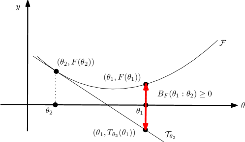
Figure 2: Illustration of the univariate Bregman divergence as the ordinate gap (‘vertical’ gap) evaluated at $\theta_{1}$ between the graph plot $\mathcal{F}$ and the tangent line $\mathcal{T}_{\theta_{2}}$ to $\mathcal{F}$ at $\theta_{2}$.

Now let us observe that we may relax the tangent line $\mathcal{T}_{\theta_{2}}$ to a chord line (or secant) $\mathcal{C}_{\theta_{1},\theta_{2}}^{\alpha,\beta}=\mathcal{C}_{(\theta_{1}\theta_{2})_{\alpha},(\theta_{1}\theta_{2})_{\beta}}$ passing through the points $((\theta_{1}\theta_{2})_{\alpha},F((\theta_{1}\theta_{2})_{\alpha}))$ and $((\theta_{1}\theta_{2})_{\beta},F((\theta_{1}\theta_{2})_{\beta}))$ for $\alpha,\beta\in(0,1)$ with $\alpha\not=\beta$ (with corresponding Cartesian equation $C_{(\theta_{1}\theta_{2})_{\alpha},(\theta_{1}\theta_{2})_{\beta}}$), and still get a non-negative vertical gap between $(\theta_{1},F(\theta_{1}))$ and $(\theta_{1},C_{(\theta_{1}\theta_{2})_{\alpha},(\theta_{1}\theta_{2})_{\beta}}(\theta_{1}))$ (because any line intersects a convex in at most two points). By construction, this vertical gap is smaller than the gap measured by the ordinary Bregman divergence. This yields the Bregman chord divergence ($\alpha,\beta\in(0,1]$, $\alpha\not=\beta$):

$$B_{F}^{\alpha,\beta}(\theta_{1}:\theta_{2}):=F(\theta_{1})-C_{F}^{(\theta_{1}\theta_{2})_{\alpha},(\theta_{1}\theta_{2})_{\beta}}(\theta_{1})\leq B_{F}(\theta_{1}:\theta_{2}),$$ (24)

illustrated in Figure 3. By expanding the chord equation and massaging the equation, we get the formula:

$$B_{F}^{\alpha,\beta}(\theta_{1}:\theta_{2}):=$$

$$F(\theta_{1})-\Delta_{F}^{\alpha,\beta}(\theta_{1},\theta_{2})(\theta_{1}-(\theta_{1}\theta_{2})_{\alpha})-F((\theta_{1}\theta_{2})_{\alpha}),$$

$$F(\theta_{1})-F\left((\theta_{1}\theta_{2})_{\alpha}\right)+\frac{\alpha\left\{{F\left((\theta_{1}\theta_{2})_{\alpha}\right)-F\left((\theta_{1}\theta_{2})_{\beta}\right)}\right\}}{\beta-\alpha},$$

where

$$\Delta_{F}^{\alpha,\beta}(\theta_{1},\theta_{2}):=\frac{F((\theta_{1}\theta_{2})_{\alpha})-F((\theta_{1}\theta_{2})_{\beta})}{(\theta_{1}\theta_{2})_{\alpha}-(\theta_{1}\theta_{2})_{\beta}},$$

is the slope of the chord, and since $(\theta_{1}\theta_{2})_{\alpha}-(\theta_{1}\theta_{2})_{\beta}=(\beta-\alpha)(\theta_{1}-\theta_{2})$ and $\theta_{1}-(\theta_{1}\theta_{2})_{\alpha}=\alpha(\theta_{1}-\theta_{2})$.

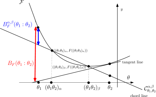
Figure 3: The Bregman chord divergence $B_{F}^{\alpha,\beta}(\theta_{1}:\theta_{2})$.

Notice the symmetry:

$$B_{F}^{\alpha,\beta}(\theta_{1}:\theta_{2})=B_{F}^{\beta,\alpha}(\theta_{1}:\theta_{2}).$$

We have asymptotically:

$$\lim_{\alpha\rightarrow 1,\beta\rightarrow 1}B_{F}^{\alpha,\beta}(\theta_{1}:\theta_{2})=B_{F}(\theta_{1}:\theta_{2}).$$

When $\alpha\rightarrow\beta$, the Bregman chord divergences yields a subfamily of Bregman tangent divergences: $B_{F}^{\alpha}(\theta_{1}:\theta_{2})=\lim_{\beta\rightarrow\alpha}B_{F}^{\alpha,\beta}(\theta_{1}:\theta_{2})\leq B_{F}(\theta_{1}:\theta_{2})$. We consider the tangent line $\mathcal{T}_{(\theta_{1}\theta_{2})_{\alpha}}$ at $(\theta_{1}\theta_{2})_{\alpha}$ and measure the ordinate gap at $\theta_{1}$ between the function plot and this tangent line:

$$B_{F}^{\alpha}(\theta_{1}:\theta_{2}) := F(\theta_{1})-F\left((\theta_{1}\theta_{2})_{\alpha}\right)-\left(\theta_{1}-(\theta_{1}\theta_{2})_{\alpha}\right)^{\top}\nabla F\left((\theta_{1}\theta_{2})_{\alpha}\right),$$ (25)

$$= F(\theta_{1})-F\left((\theta_{1}\theta_{2})_{\alpha}\right)-\alpha(\theta_{1}-\theta_{2})^{\top}\nabla F\left((\theta_{1}\theta_{2})_{\alpha}\right),$$

for $\alpha\in(0,1]$. The ordinary Bregman divergence is recovered when $\alpha=1$. Notice that the mean value theorem yields $\Delta_{F}^{\alpha,\beta}(\theta_{1},\theta_{2})=F^{\prime}(\xi)$ for $\xi\in(\theta_{1},\theta_{2})$. Thus $B_{F}^{\alpha,\beta}(\theta_{1}:\theta_{2})=B_{F}^{\xi}(\theta_{1}:\theta_{2})$ for $\xi\in(\theta_{1},\theta_{2})$. Letting $\beta=1$ and $\alpha=1-\epsilon$ (for small values of $1>\epsilon>0$), we can approximate the ordinary Bregman divergence by the Bregman chord divergence without requiring to compute the gradient: $B_{F}(\theta_{1}:\theta_{2})\simeq_{\epsilon\rightarrow 0}B_{F}^{1-\epsilon,1}(\theta_{1}:\theta_{2})$.

Figure 4 displays some snapshots of an interactive demo program that illustrates the impact of $\alpha$ and $\beta$ for defining the Bregman chord divergences for the quadratic and Shannon generators.

	Bregman chord divergence	Bregman tangent divergence
Quadratic
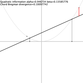
	(a)	(b)
Shannon
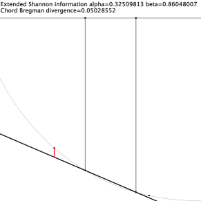
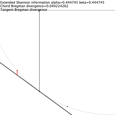
	(c)	(d)

Figure 4: The univariate Bregman chord divergences and Bregman tangent divergences for the quadratic and Shannon information generators.

4 The multivariate Bregman chord divergence

When the generator is separable [3], i.e., $F(x)=\sum_{i}F_{i}(x_{i})$ for univariate generators $F_{i}$, we extend easily the Bregman chord divergence as: $B_{F}^{\alpha,\beta}(\theta:\theta^{\prime})=\sum_{i}B_{F_{i}}^{\alpha,\beta}(\theta_{i}:\theta^{\prime}_{i})$. Otherwise, we have to carefully define the notion of “slope” for the multivariate case. An example of such a non-separable multivariate generator is the Legendre dual of the Shannon negentropy: The log-sum-exp function $F(\theta)=\log(1+\sum_{i}e^{\theta_{i}})$.

Given a multivariate (non-separable) Bregman generator $F(\theta)$ with $\Theta\subseteq\mathbb{R}^{D}$ and two prescribed distinct parameters $\theta_{1}$ and $\theta_{2}$, consider the following univariate function, for $\lambda\in\mathbb{R}$:

$$F_{\theta_{1},\theta_{2}}(\lambda):=F\left((1-\lambda)\theta_{1}+\lambda\theta_{2}\right)=F\left(\theta_{1}+\lambda(\theta_{2}-\theta_{1})\right),$$ (26)

with $F_{\theta_{1},\theta_{2}}(0)=F(\theta_{1})$ and $F_{\theta_{1},\theta_{2}}(1)=F(\theta_{2})$.

The functions $\{F_{\theta_{1},\theta_{2}}\}$ are strictly convex and univariate Bregman generators.

Proof.

To prove the strict convexity of a univariate function $G$, we need to show that for any $\alpha\in(0,1)$, we have

$$G((1-\alpha)x+\alpha y)<(1-\alpha)G(x)+\alpha G(y).$$

$$F_{\theta_{1},\theta_{2}}((1-\alpha)\lambda_{1}+\alpha\lambda_{2}) = F\left(\theta_{1}+((1-\alpha)\lambda_{1}+\alpha\lambda_{2})(\theta_{2}-\theta_{1})\right),$$

$$= F((1-\alpha)(\lambda_{1}(\theta_{2}-\theta_{1})+\theta_{1})+\alpha((\lambda_{2}(\theta_{2}-\theta_{1})+\theta_{1}))),$$

$$< (1-\alpha)F(\lambda_{1}(\theta_{2}-\theta_{1})+\theta_{1})+\alpha F((\lambda_{2}(\theta_{2}-\theta_{1})+\theta_{1})),$$

$$< (1-\alpha)F_{\theta_{1},\theta_{2}}(\lambda_{1})+\alpha F_{\theta_{1},\theta_{2}}(\lambda_{2}).$$

∎

Then we define the multivariate Bregman chord divergence by applying the definition of the univariate Bregman chord divergence of on these families of univariate Bregman generators:

$$B_{F}^{\alpha,\beta}(\theta_{1}:\theta_{2}):=B_{F_{\theta_{1},\theta_{2}}}^{\alpha,\beta}(0:1),$$ (27)

Since $(01)_{\alpha}=\alpha$ and $(01)_{\beta}=\beta$, we get:

$$B_{F}^{\alpha,\beta}(\theta_{1}:\theta_{2})$$

$$=F_{\theta_{1},\theta_{2}}(0)+\frac{\alpha(F_{\theta_{1},\theta_{2}}(\alpha)-F_{\theta_{1},\theta_{2}}(\beta))}{\beta-\alpha}-F_{\theta_{1},\theta_{2}}(\alpha),$$

$$F(\theta_{1})-F\left((\theta_{1}\theta_{2})_{\alpha}\right)-\frac{\alpha\left(F\left((\theta_{1}\theta_{2})_{\beta}\right)-F\left((\theta_{1}\theta_{2})_{\alpha}\right)\right)}{\beta-\alpha},$$

in accordance with the univariate case. Since $(\theta_{1}\theta_{2})_{\beta}=(\theta_{1}\theta_{2})_{\alpha}-(\beta-\alpha)(\theta_{2}-\theta_{1})$, we have the first-order Taylor expansion:

$$F\left((\theta_{1}\theta_{2})_{\beta}\right)\simeq_{\beta\simeq\alpha}F\left((\theta_{1}\theta_{2})_{\alpha}\right)-(\beta-\alpha)(\theta_{2}-\theta_{1})^{\top}\nabla F\left((\theta_{1}\theta_{2})_{\alpha}\right).$$

Therefore, we have:

$$\frac{\alpha\left(F\left((\theta_{1}\theta_{2})_{\beta}\right)-F\left((\theta_{1}\theta_{2})_{\alpha}\right)\right)}{\beta-\alpha}\simeq-\alpha(\theta_{2}-\theta_{1})^{\top}\nabla F\left((\theta_{1}\theta_{2})_{\alpha}\right).$$

This proves that $\lim_{\beta\rightarrow\alpha}B_{F}^{\alpha,\beta}(\theta_{1}:\theta_{2})=B_{F}^{\alpha}(\theta_{1}:\theta_{2})$.

Notice that the Bregman chord divergence does not require to compute the gradient $\nabla F$ The “slope term” in the definition is reminiscent to the $q$-derivative [17] (quantum/discrete derivatives). However the $(p,q)$-derivatives [17] are defined with respect to a single reference point while the chord definition requires two reference points.

5 Conclusion and perspectives

We geometrically designed a new class of distances using two scalar parameters, termed the Bregman chord divergence, and its one-parametric subfamily, the Bregman tangent divergences that includes the ordinary Bregman divergence. This generalization allows one to easily fine-tune Bregman divergences in applications by adjusting smoothly one or two (scalar) knobs. Moreover, by choosing $\alpha=1-\epsilon$ and $\beta=1$ for small $\epsilon>0$, the Bregman chord divergence $B_{F}^{1-\epsilon,1}(\theta_{1}:\theta_{2})$ lower bounds closely the Bregman divergence $B_{F}(\theta_{1}:\theta_{2})$ without requiring to compute the gradient (a different approximation without gradient is $\frac{1}{\epsilon}J_{F}^{\epsilon}(\theta_{2}:\theta_{1})$). We expect that this new class of distances brings further improvements in signal processing and information fusion applications [28] (e.g., by tuning $B_{F_{\mathrm{KL}}}^{\alpha,\beta}$ or $B_{F_{\mathrm{IS}}}^{\alpha,\beta}$). While the Bregman chord divergence defines an ordinate gap on the exterior of the epigraph, the Jensen chord divergence [22] defines the gap inside the epigraph of the generator. In future work, the information-geometric structure induced by the Bregman chord divergences (curved) shall be investigated from the viewpoint of gauge theory [21] and in constrast with the dually flat structures of Bregman manifolds [3].

Java™ Source code is available for reproducible research.

References

- [1] Syed Mumtaz Ali and Samuel D. Silvey. A general class of coefficients of divergence of one distribution from another. Journal of the Royal Statistical Society. Series B (Methodological), pages 131–142, 1966.
- [2] Shun-ichi Amari. -divergence is unique, belonging to both -divergence and Bregman divergence classes. IEEE Transactions on Information Theory, 55(11):4925–4931, 2009.
- [3] Shun-ichi Amari. Information geometry and its applications. Springer, 2016.
- [4] Arindam Banerjee, Xin Guo, and Hui Wang. On the optimality of conditional expectation as a Bregman predictor. IEEE Transactions on Information Theory, 51(7):2664–2669, 2005.
- [5] Arindam Banerjee, Srujana Merugu, Inderjit S Dhillon, and Joydeep Ghosh. Clustering with Bregman divergences. Journal of machine learning research, 6(Oct):1705–1749, 2005.
- [6] Michèle Basseville. Divergence measures for statistical data processing: An annotated bibliography. Signal Processing, 93(4):621–633, 2013.
- [7] Lev M Bregman. The relaxation method of finding the common point of convex sets and its application to the solution of problems in convex programming. USSR computational mathematics and mathematical physics, 7(3):200–217, 1967.
- [8] Jacob Burbea and C. Rao. On the convexity of some divergence measures based on entropy functions. IEEE Transactions on Information Theory, 28(3):489–495, 1982.
- [9] Andrzej Cichocki, Hyekyoung Lee, Yong-Deok Kim, and Seungjin Choi. Non-negative matrix factorization with -divergence. Pattern Recognition Letters, 29(9):1433–1440, 2008.
- [10] Thomas M Cover and Joy A Thomas. Elements of information theory. John Wiley & Sons, 2012.
- [11] Imre Csiszár. Information-type measures of difference of probability distributions and indirect observation. studia scientiarum Mathematicarum Hungarica, 2:229–318, 1967.
- [12] Imre Csiszár. Why least squares and maximum entropy? an axiomatic approach to inference for linear inverse problems. The annals of statistics, 19(4):2032–2066, 1991.
- [13] Michel Marie Deza and Elena Deza. Encyclopedia of distances. In Encyclopedia of Distances, pages 1–583. Springer, 2009.
- [14] Cédric Févotte. Majorization-minimization algorithm for smooth Itakura-Saito nonnegative matrix factorization. In Acoustics, Speech and Signal Processing (ICASSP), 2011 IEEE International Conference on, pages 1980–1983. IEEE, 2011.
- [15] Johan Ludwig William Valdemar Jensen. Sur les fonctions convexes et les inégalités entre les valeurs moyennes. Acta mathematica, 30(1):175–193, 1906.
- [16] Jiantao Jiao, Thomas A Courtade, Albert No, Kartik Venkat, and Tsachy Weissman. Information measures: the curious case of the binary alphabet. IEEE Transactions on Information Theory, 60(12):7616–7626, 2014.
- [17] Victor Kac and Pokman Cheung. Quantum calculus. Springer Science & Business Media, 2001.
- [18] Krzysztof C. Kiwiel. Proximal minimization methods with generalized Bregman functions. SIAM journal on control and optimization, 35(4):1142–1168, 1997.
- [19] Minami Mihoko and Shinto Eguchi. Robust blind source separation by beta divergence. Neural computation, 14(8):1859–1886, 2002.
- [20] Dharmendra S. Modha and W. Scott Spangler. Feature weighting in -means clustering. Machine learning, 52(3):217–237, 2003.
- [21] Jan Naudts and Jun Zhang. Rho–tau embedding and gauge freedom in information geometry. Information Geometry, pages 1–37, 2018.
- [22] Frank Nielsen. The chord gap divergence and a generalization of the Bhattacharyya distance. In IEEE International Conference on Acoustics, Speech and Signal Processing (ICASSP), pages 2276–2280, April 2018.
- [23] Frank Nielsen and Sylvain Boltz. The Burbea-Rao and Bhattacharyya centroids. IEEE Transactions on Information Theory, 57(8):5455–5466, 2011.
- [24] Frank Nielsen and Richard Nock. Skew Jensen-Bregman voronoi diagrams. In Transactions on Computational Science XIV, pages 102–128. Springer, 2011.
- [25] Frank Nielsen and Richard Nock. On the geometry of mixtures of prescribed distributions. In IEEE International Conference on Acoustics, Speech and Signal Processing (ICASSP), pages 2861–2865. IEEE, 2018.
- [26] M. C. Pardo and Igor Vajda. About distances of discrete distributions satisfying the data processing theorem of information theory. IEEE transactions on information theory, 43(4):1288–1293, 1997.
- [27] Matus Telgarsky and Sanjoy Dasgupta. Agglomerative Bregman clustering. In Proceedings of the 29th International Conference on International Conference on Machine Learning, pages 1011–1018. Omnipress, 2012.
- [28] Murat Üney, Jérémie Houssineau, Emmanuel Delande, Simon J. Julier, and Daniel E. Clark. Fusion of finite set distributions: Pointwise consistency and global cardinality. CoRR, abs/1802.06220, 2018.
- [29] Jun Zhang. Divergence function, duality, and convex analysis. Neural Computation, 16(1):159–195, 2004.